IEEE TRANSACTIONS ON AUTOMATIC CONTROL, VOL. 42, NO. 6, JUNE 1997 835

Now, let us state the main contribution of the paper. The necessaryand sufficient conditions in the following theorem hold forall centerquasi-polynomialsq(z; a�) (n > 1) and radii r satisfying theAssumption 2.2 in the familyQw;r.

Theorem 4.3: The stability of the eight one-parameter families ofquasi-polynomials

q(z;a�)� �r

w0m

� (1� �)r

w1m

z e� z (29)

q(z;a�)� �r

w(n�1)m

� (1� �)r

wnm

z zn�1

e� z

;

� 2 [0; 1]

implies the stability of the familyQw;r if and only if the conditions(26)–(28) in Lemma 4.1 and Lemma 4.2 are satisfied.

Proof: The proof follows from Proposition 2.1, Lemma 4.1, andLemma 4.2.

Remark 4.4: Note that similar conditions to (26)–(28) can bestated so that the real weighted diamond of quasi-polynomials enjoysa 12-, a 16-, or more generally, a “weak”-edge property.

ACKNOWLEDGMENT

The authors would like to thank the referees for many helpfulcomments on the content of this paper. They also would like to thankDr. A. D. B. Paice for improving the English in the paper.

REFERENCES

[1] B. R. Barmish, R. Tempo, C. V. Hollot, and H. I. Kang, “An extremepoint result for robust stability of a diamond of polynomials,”IEEETrans. Automat. Contr., vol. 37, pp. 1460–1462, 1992.

[2] R. Bellman and K. L. Cook,Differential-Difference Equations. NewYork: Academic, 1963.

[3] M. Fu, A. W. Olbrot, and M. P. Polis, “Robust stability for time-delaysystems: The edge theorem and graphical tests,”IEEE Trans. Automat.Contr., vol. 34, pp. 813–820, 1989.

[4] J. Hocherman, V. L. Kharitonov, J. Kogan, and E. Zeheb, “On thestability of quasi-polynomials with weighted diamond coefficients,”Multidimensional Syst. Signal Processing, vol. 5, pp. 397–418, 1994.

[5] J. Hocherman, J. Kogan, and E. Zeheb, “Simple stability criterionfor quasi-polynomial families with uncertain coefficients and uncertaindelays,” inProc. 32nd IEEE Conf. Decision Contr., San Antonio, Texas,Dec. 15–17, 1993.

[6] V. L. Kharitonov and R. Tempo, “On the stability of a weighted diamondof polynomials,”Syst. Contr. Lett., vol. 22, pp. 5–7, 1994.

[7] V. L. Kharitonov and A. P. Zhabko, “Stability of convex hull ofquasi-polynomials,” inRobustness of Dynamic Systems with ParameterUncertainties. Basel: Birkhauser Verlag, 1992, pp. 63–69.

[8] J. Kogan, “Hurwitz stability of weighted diamond polynomials,”Syst.Contr. Lett., vol. 22, pp. 303–312, 1994.

[9] R. Tempo, “A dual result to Kharitonov’s theorem,”IEEE Trans.Automat. Contr., vol. 35, pp. 195–198, 1990.

Robust Control System Design Using RandomSearch and Genetic Algorithms

Christopher I. Marrison and Robert F. Stengel

Abstract—Random search and genetic algorithms find compensators tominimize stochastic robustness cost functions. Statistical tools are incor-porated in the algorithms, allowing intelligent decisions to be based on“noisy” Monte Carlo estimates. The genetic algorithm includes clusteringanalysis to improve performance and is significantly better than therandom search for this application. The algorithm is used to design acompensator for a benchmark problem, producing a control law withexcellent stability and performance robustness.

Index Terms—Genetic algorithms, probabilistic methods, robust controldesign and analysis.

I. INTRODUCTION

Compensators that perform sufficiently well in the presence ofplant parameter variations are said to berobust. Stochastic robustnessanalysis is a practical method for quantifying compensator robustness[1]. The stochastic robustness metric characterizes a compensator,G,as theprobability that the closed-loop system will have unacceptableperformance in the presence of possible parameter variations. Theprobability,P , can be defined as the integral of an indicator functionover the space of expected parameter variations

P =V

I[H(v); G]pr(v)dv (1)

whereH is the plant structure,V is the space of possible parametervariations,v is a point inV , and pr(v) is the probability densityfunction. I[�] is a binary indicator function that equals one, ifH(v)and G form an unacceptable system, and is zero otherwise. Thedesigner decides the definition of “unacceptable.” For example, itcould mean instability, violation of a response envelope, excess useof control, or a combination of qualities. This metric deals equallywell with linear, nonlinear, time-invariant, and time-varying systems.

In finding the best compensator, there may be tradeoffs betweenthose that minimize one performance metric and those that minimizea different metric. Tradeoffs can be formalized by combining theprobabilities in a scalar robustness cost function

J = fcn(P1; P2; � � �): (2)

Each design point,d; (d 2 D); defines a compensator,G(d). WithIj ; H; V; andpr(v) fixed, the problem is to find the value ofd thatminimizes J(d).

In most applications, (1) cannot be integrated analytically. Apractical alternative is to use Monte Carlo Evaluation (MCE) [2] withpr(v) shaping the random samplings of values forv, and individualselections for each trial denoted byvm. The trials are repeated for

Manuscript received January 20, 1995; revised January 12, 1996 and July25, 1996. This work was supported in part by the FAA and NASA underGrant NGL 31-001-252.

C. I. Marrison is with Oliver, Wyman & Company, New York, NY 10103USA.

R. F. Stengel is with the Department of Mechanical and AerospaceEngineering, Princeton University, Princeton, NJ 08544 USA.

Publisher Item Identifier S 0018-9286(97)03389-8.

0018–9286/97$10.00 1997 IEEE

836 IEEE TRANSACTIONS ON AUTOMATIC CONTROL, VOL. 42, NO. 6, JUNE 1997

N samples inV . The estimates are then

Pj(d) =1

N

N

m=1

Ij [H(vm);G(d)] (3)

J(d) = fcn[P (d)1; P (d)2; � � �]: (4)

J approachesJ in the limit asN ! 1.In [3], robust linear-quadratic-Gaussian (LQG) compensators for a

benchmark control problem were found using MCE and a sequenceof line searches. The compensators were exceedingly robust, but thesearch algorithm was inefficient, requiring many MCE’s. This paperdevelops efficient algorithms for designing robust controllers usingrandom search and genetic algorithms (GA).

II. RANDOM SEARCH AND GENETIC ALGORITHMS

AS USED ON DETERMINISTIC FUNCTIONS

Although the random search is inefficient, it is simple and oftenused as a standard for comparison with other searches [4]. Thedesigner initiates the random search by defining the limits of thesearch space,D. A random number generator selects pointsdk withinD, wherek = 1 � � �Ns, andNs is the number of search points. Thevalue ofJ(dk) is tested for eachk, and the point giving the lowestvalue is taken to be the estimate of the global minimizer,d

�.Genetic algorithms [5]–[7] are randomized adaptive search meth-

ods that process a large number of search points at each step andsplice the best of the old search points together to produce a newset of points. A GA has two significant advantages for searching astochastic robustness cost function: randomization within the searchmethod makes the algorithms robust to errors inJ , and the splicingproduces implicit parallelism, which limits computational complexity.

The GA manipulates a population of binary vectors represent-ing points in D. There are four operations: evaluation, selection,crossover, and mutation. The initial population is formed by randomlyselecting a number(Npop) of vectorsdk (k = 1 � � �Npop) from D.J(dk) is evaluated and used to select pairs of vectors. The selectionprocedure is probabilistic and is more likely to choose vectors givinggood values ofJ . Several selection procedures are available [8];tournament selectionis used here. Two members of the population areselected, their corresponding values ofJ(dk) are compared, and themember with the better value is retained. A second vector is selectedin the same fashion, and crossover is performed on the two retainedvectors. A random point is chosen along vectors, separating eachvector into a “head” and a “tail,” and the two tails are swapped. Aftercrossover, the vectors may be mutated, whereby any element in thevector may be altered with probabilityPm. Selection, crossover, andmutation are carried outNpop=2 times to generate a new population.Regeneration is repeated until the population converges.

A real-number genetic algorithm (used here) allows each elementof d to be continuous, but it requires two stages of mutation toaffect the local and global search. The first mutation, a multiplicativechange, provides the local search

d0

m;k = dm;kbU(�1;1) (5)

wheredm;k is themth element ofdk; b is a base number, typicallyequal to two, andU(�1; 1) is a random variable from a uniformdistribution in�1. The global search is given by

d0

m;k = dm;k + U(�1; 1)[max(dm)�min(dm)] (6)

wheremax(dm) and min(dm) define the limits of directionm ofD. Each of these mutations may be given a different probability ofoccurring.

Elite selection and clusteringimprove search efficiency. Eliteselection retains one or more of the best members of the population

and passes them directly into the new generation without crossoveror mutation. This ensures that the best solution is not lost. Clustering[9] can create a “super-elite” member to pass into the new generationfrom groups of vectors that lie close to the global minimum. Thecentroid is passed to the new generation as a super-elite member.

Values must be chosen for the search parameters within theGA. In the above algorithm these parameters are: the number ofpopulation members,Npop, the probability of global mutation,Pmg,the probability of local mutation,Pml, the base for local mutation,b,and the initial number of MCE’s,NMCE0.

III. STATISTICAL CONSIDERATIONS

If the objective function were evaluated without error, the randomsearch would easily choose the best of the tested points and eliminateall inferior points. However, an MCE allows errors inJ. A searchpoint cannot be eliminated unless there is a significant differencebetweenJ for the given point andJ for the best point. For efficientrandom search, significant difference must be identified using aminimal number of MCE’s.

Confidence intervalsbound the expected error of an estimate. Theprobability that the true value ofP lies in the interval[L;U ] is

Pr[L � P � U ] = 1� �: (7)

Analytic derivation of confidence intervals is possible only forsimple probability distributions.Bootstrapping [10] estimates thedistribution of J by repeatedly simulating the estimation processwithout reassessing the original function.J 0 is repeatedly estimated as

J0= fcn(P

0

1; P0

2; P0

3; � � �) (8)

whereP 0

j is sampled from a binomial distribution with a mean ofPj .The values ofJ 0 are ordered, the bottom100� percentile is taken asL, and the100(1� �) percentile definesU .

In searching the stochastic cost function, pairs of compensators,G(da) andG(db), are compared on the basis ofestimatesrather thanactual costs. If�J � J(da) � J(db) and �J is bounded by aconfidence interval that does not include zero, there is a statisticallysignificant difference betweenG(da) and G(db). The constructionof a confidence interval for�J could be based on the confidenceintervals forJ(da); J(db) and the Bonferroni inequality, or on theStudentt distribution [11]. These methods are conservative in thisapplication because they assume the samples are independent. Tighterconfidence bounds on�J can be constructed if the same samplepoints are used for the MCE of bothJ(da) andJ(db). Although thetechnique is straightforward, exploiting it is complex; for illustration,consider the simple cost functionJ = P1. The difference betweentwo compensators is then

�J = Ja � Jb = P1;a � P1;b

=V

fI1[H(v);G(da)]� I1[H(v);G(db)]gdv: (9)

V has four overlapping subvolumes

Va: v 2 Va ! I1[H(v);G(da)] = 1

Va=: v 2 Va= ! I1[H(v);G(da)] = 0

Vb: v 2 Vb ! I1[H(v);G(db)] = 1

Vb=: v 2 Vb= ! I1[H(v);G(db)] = 0:

(10)

Va is the sub-volume of the plant parameter space in which the closed-loop performance with compensatorda is unacceptable, andVa= isthe space where it is acceptable.Vb andVb= are described similarly.Combining these spaces gives (Fig. 1)

Va\b � Va \ Vb; Va\b= � Va \ Vb=

Va=\b � Va= \ Vb; Va=\b=;� Va= \ Vb=:(11)

IEEE TRANSACTIONS ON AUTOMATIC CONTROL, VOL. 42, NO. 6, JUNE 1997 837

Fig. 1. Division of space according to metrics.

The probabilities in (9) can be restated as

P1;a =

V

I1[H(v);G(da)]pr(v)dv

=

V

I1[�]pr(v)dv +

V

I1[�]pr(v)dv: (12)

The indicator functionI1[H(v);G(da)] equals one inVa and zeroin Va=, and (12) becomes

P1;a =

V

pr(v)dv

=

V

pr(v)dv+

V

pr(v)dv

= Pa\b + Pa\b=: (13)

Pa\b is the probability of the plant parameter vector,v, being ina subvolume, where bothda anddb are unacceptable.Pa\b= is theprobability of being in a subvolume whereda is unacceptable anddb is acceptable. With these definitions, (9) is

�J = (Pa\b + Pa\b=)� (Pb\a + Pb\a=) (14)

and it is estimated as

�J = (Pa\b + Pa\b=)� (Pb\a + Pb\a=): (15)

If the sampling for each probability is independent, then the variancein the Monte Carlo estimate of�J is the sum of variances [11]

�2

�J = �2

P + �2

P + �2

P + �2

P : (16)

Alternatively, if the sample points are the same for bothG(da) andG(db), thenPa\b � Pb\a; therefore, (15) and (16) simplify to

�J = Pa\b= � Pb\a= (17)

�2

�J = �2

P + �2

P : (18)

Eliminating�2P

is significant ifda anddb are close together andhave similar performance.

Repeating sample points reduces the estimation error and improvesthe search. In many cases it is possible to construct tighter confidenceintervals around�J , allowing decisions to be based on fewerevaluations. WithJ = P1, it is a simple matter to constructconfidence intervals by bootstrapping. The procedure repeatedlysimulates�J 0 as

�J0= P

0

a\b= � P0

a=\b (19)

whereP 0

a\b= is a random number from the binomial distribution withmeanP 0

a\b=. For more complex cost functions,�J must be expandedto expose the elements that contain the identical probability estimates,Pa\b and Pb\a, which cancel in the construction of confidenceintervals. Consider the quadratic cost functionJ = j wjP

2

j ; then

�J =

j

wj P2

j;a � P2

j;b

=

j

wj P2

j;a\b= � P2

j;b\a= + 2Pj;a\b(Pj;a\b= � Pj;b\a=) : (20)

This process eliminates the variation in the random search due toP 2

j;a\b and Pj;b\a.The GA selection procedure is based on differences between cost

estimates. Statistical tools are needed to supply sufficiently accurateestimates without using more MCE’s than are necessary. Errors inJ

do not affect selection if the error is smaller than the true difference.This principle guides the selection ofN , the number of evaluationsused to assess each new member. The dispersion of the top 25% ofthe population is characterized by

�2

pop =1

Npop=4� 1

N =4

k=1

[J(dk)� �J ]2 (21)

�J =1

Npop=4

N =4

k=1

�J(dk): (22)

The mean variance in the individual estimates ofJ is

��2

J =1

Npop=4

N =4

k=1

��2

J(d ) (23)

where �2J(d )

denotes the variance of estimateJ(dk). �2J(d )is

obtained by the bootstrapping procedure [10]. Relating (21) to (23)allows a desirable magnitude of��J to be defined as��pop, where�is a positive number on the order of one, chosen by the designer.

The desired��J can be related to the required number of MCE’s.The stochastic robustness metrics are binary, andP has abinomialprobability distribution [11] with standard deviation

�P =P � P 2

N(24)

whereP is the true probability. The standard deviation ofJ thereforevaries inversely with

pN . If one pairing ofN and�J is known, then

theN required to achieve the desired level of��J is

Nreq = Ncur ��J =��J2

: (25)

IV. I NCORPORATING STATISTICAL

TOOLS INTO THE SEARCH ALGORITHMS

In the random search, a number of MCE’s are carried out foreachdk, using the same sample points to test each compensator.The search estimates the best search point,dmin, as the one withJ(dk) = minj [J(dj)], and for the other compensators calculates�Jk = J(dk) � J(dmin). Bootstrapping is used to calculate thelower bound on the confidence interval for�Jk. This lower boundis L�Jk. If L�Jk is greater than zero, then there is a significantdifference betweenJ(dk) and J(dmin). When the difference isstatistically significant,dk can be eliminated from the search, i.e.,if L�Jk is greater than zero,dk is eliminated.

The reduced population is subjected to additional MCE’s. The mostefficient number of evaluations is the number that will increase theaccuracy of each estimated difference,�Jk, just enough to eliminatethe next test point. This number is estimated by comparing the

838 IEEE TRANSACTIONS ON AUTOMATIC CONTROL, VOL. 42, NO. 6, JUNE 1997

Fig. 2. Performance of the search algorithms on a 24-parameter test function.

current width of the confidence interval around�Jk with the intervalrequired to be certain that�Jk is greater than zero, i.e., that the lowerboundL�Jk is greater than or equal to zero. The current differencebetween�Jk and the lower bound is(�Jk�L�Jk), and the requireddifference is equal to(�Jk � 0). From (25), the number of MCE’srequired to eliminate pointk is estimated as

Nreq;k = Ncur

�Jk � L�Jk

�Jk

2

; k = 1 � � �Ns: (26)

The number of extra evaluations required isNreq;k �Ncur.There are two possible stopping conditions for the search. The

obvious condition is that only one point remains. The other conditionis that the upper bound on all the remaining points is close to thevalue of the best point, i.e.,

maxk

[U�Jk] � (1 + �)mink

[J(dk)]: (27)

U�Jk is the upper bound on the confidence interval for�Jk, and�is a small positive number.

The number of MCE’s for each member of the new population (25)must be evaluated for the genetic algorithm. In the process, stratifiedsampling and retaining a single set of plant parameter vectors withinone generation minimizes the variance of�Jk.

V. APPLICATION TO A TEST FUNCTION

The test function maps a point in a 24-dimensional space,D, to ascalarJ(d); d 2 D. The test function is a weighted quadratic sumof three probabilities

J(d) = P 21 (d) + 0:1P 2

2 (d) + 0:1P 23 (d): (28)

P1 is the dominant term (e.g., the probability of closed-loop instabil-ity), while P2 andP3 are less critical performance metrics. Eighteenpositive functions are summed to simulate each probability [12]. Theminimizing values ofd are in a small portion of the search volume.Here,Jmax is 1.2,Jmean is 1.071, andJmin is 0.033. Only 3% ofD hasJ < 0:5, and 0.09% hasJ < 0:25.

To simulate the effects of MCE, whenPi(d) is sampled,Ii(d)returns the value one or zero. A random value is chosen from auniform U(0; 1) distribution. If the value is less thanP (d); Ii(d)returns one; otherwise, zero is returned.

The search performance is defined as the average value ofJ(dmin),where dmin is the final selected value. The average value wascalculated by running the entire search algorithm 400 times andtaking the mean of the best point values. The performance depends

TABLE ICONSTANTS OF THE GENETIC ALGORITHM

on the number of search points chosen (Fig. 2). With 104 functionevaluations, the random search achieves an average final value(E[J�nal]) of 0.236 (only 0.055% ofD hasJ < 0:236).

The genetic algorithms also were run 400 times against the testfunction. The minimum value ofJ was recorded when the search hadused more than 2000, 4000, 6000, 8000, and 104 MCE’s. The baselinealgorithm uses an initial set of guesses for the parameters withinthe GA and does not use clustering or elite selection.E[J�nal] =0:183 for a mean number of 104 evaluations. Elite selection andclustering improved performance. With 104 evaluations, the averageperformance wasE[J�nal] = 0:156 (0.0035% ofD hasJ < 0:156).

Performance was enhanced by adding clustering and elite selectionand by tuning the search parameters. The initial and optimizedconstant values are listed in Table I. After 104 evaluations, therandom search achievesE[J�nal] = 0:24, whereas the GA achievesE[J�nal] = 0:11 (Fig. 2). The random search requires 104 eval-uations to achieveE[J�nal] = 0:24, while the GA requires only900 evaluations to achieve the same result, an 11-fold savings incomputation.

VI. A PPLICATION TO A BENCHMARK CONTROL PROBLEM

The genetic algorithm was used to design robust compensators fora benchmark problem [14]. The plant is a mass-spring-mass systemwith noncollocated sensor and actuator. The actuator/output transferfunction is

Huy =(k=m1m2)

s2[s2 + k(m1 +m2)=m1m2](29)

wherem1 andm2 are the masses andk is the spring constant, eachof unit value. The task is to design a compensator to commandu,given measurements ofy. There are three requirements: a nominal15-s settling time in response to a unit disturbance impulse, minimalactuator use, and maximal stability robustness whenm1;m2; andkare uncertain [15]. The plant parameters have uniform probabilitydistributions, with0:5 < k < 2; 0:5 < m1 < 1:5; and0:5 < m2 <1:5.

Stochastic robustness analysis was used to compare the robustnessof ten compensators designed by five different groups [14], [15]. Therobustness was quantified by the probability of instability,(Pi), theprobability of excessive settling time,(PTs), and the probability ofexcessive actuator use,(Pu). In [3], robust LQG regulators weredesigned using stochastic robustness metrics, and a line search wasused to find parameters that minimize a robustness cost function.Design 1 minimized a cost function defined asJ = P 2

i +0:01P 2Ts+

0:01P 2u , achievingPi = 0:0034; PTs = 0:7588; Pu = 0:1077, or

J = 0:0059. Design 1 is 1.5 times better than the best of the tencompensators in [15]. However, the synthesis of Design 1 requireda total of 701 250 MCE’s.

IEEE TRANSACTIONS ON AUTOMATIC CONTROL, VOL. 42, NO. 6, JUNE 1997 839

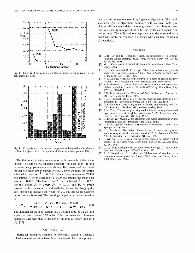
Fig. 3. Progress of the genetic algorithm in finding a compensator for thebenchmark problem.

Fig. 4. Comparison of robustness of compensators designed for a benchmarkproblem (designsA to J correspond with the designations given in [16]).

The GA found a better compensator with one-tenth of the calcu-lations. The same LQG regulator structure was used as in [3], andthe same design parameters were chosen. The progress of one run ofthe genetic algorithm is shown in Fig. 3. Over 20 runs, the searchachieved a mean ofJ = 0:0059 with a mean number of 70 400evaluations. After an average of 115 500 evaluations, the mean costwas J = 0:0056. The best of the 20 runs achievedJ = 0:0039.For this designPi = 0:019; PTs = 0:596; and Pu = 0:019

(greater stability robustness could easily be obtained by changing thecost function to increase the weight onPi, but this would sacrificeperformance robustness). The resulting compensator transfer functionis

Gyu =1:53(s� 5:88)(s+ 0:149)(s+ 0:479)

(s+ 0:693)(s2 + 1:54s+ 5:45)(s2 + 2:59s+ 1:69): (30)

The nominal closed-loop system has a settling time of 13.2 s anda peak actuator use of 0.52 units. This compensator’s robustnesscompares well with that of the earlier designs, as shown in Fig. 4[3], [15].

VII. CONCLUSION

Statistical principles required to efficiently search a stochasticrobustness cost function have been developed. The principles are

incorporated in random search and genetic algorithms. This workshows that genetic algorithms, combined with statistical tools, pro-vide an efficient method for searching a stochastic robustness costfunction, opening new possibilities for the synthesis of robust con-trol systems. The utility of our approach was demonstrated on abenchmark problem, resulting in a design with excellent robustnesscharacteristics.

REFERENCES

[1] L. R. Ray and R. F. Stengel, “Stochastic robustness of linear-time-invariant control systems,”IEEE Trans. Automat. Contr., vol. 36, pp.82–87, Jan. 1991.

[2] M. H. Kalos and P. A. Whitlock,Monte Carlo Methods. New York:Wiley, 1986.

[3] C. I. Marrison and R. F. Stengel, “Stochastic robustness synthesisapplied to a benchmark problem,”Int. J. Robust Nonlinear Contr., vol.5, no. 1, pp. 13–31, Jan. 1995.

[4] K. A. DeJong, “Analysis of the behavior of a class of genetic adaptivesystems,” Ph.D. dissertation, Univ. Michigan, Ann Arbor, 1975.

[5] K. Krishnakumar, “Genetic algorithms: An introduction and an overviewof their capabilities,” inProc. 1992 AIAA GNC Conf., Hilton Head, Aug.1992, pp. 728–738.

[6] J. Holland,Adaptation in Natural and Artificial Systems. Ann Arbor,MI: Univ. Michigan Press, 1975.

[7] J. M. Fitzpatrick and J. J. Grefenstette, “Genetic algorithms in noisyenvironments,”Machine Learning, vol. 3, pp. 101–120, 1988.

[8] D. E. Goldberg,Genetic Algorithms in Search, Optimization, and Ma-chine Learning. Reading, MA: Addison Wesley, 1989.

[9] A. A. Torn, “Cluster analysis using seed points and density-determinedhyperspheres as an aid to global optimization,”IEEE Trans. Syst. Man.Cybern., vol. 7, pp. 610–616, Aug. 1977.

[10] B. Efron, The Jackknife, the Bootstrap and Other Resampling Plans.Philadelphia, PA: Soc. Industrial Appl. Math., 1985.

[11] L. Sachs,Applied Statistics: A Handbook of Techniques. New York:Springer-Verlag, 1984.

[12] C. I. Marrison, “The design of control laws for uncertain dynamicsystems using stochastic robustness metrics,” Ph.D. dissertation, MAE-2001-T, Princeton Univ., Princeton, NJ, Jan. 1995.

[13] B. Wie and D. S. Bernstein, “A benchmark problem for robust controldesign,” inProc. 1990 Amer. Contr. Conf., San Diego, CA, May 1990,pp. 961–962.

[14] , “Benchmark problems for robust control design,”J. Guid. Contr.Dyn., vol. 15, no. 5, pp. 1057–1059, Sept. 1992.

[15] R. F. Stengel and C. I. Marrison, “Robustness of solutions to abenchmark control problem,”J. Guid. Contr. Dyn, vol. 15, no. 5, pp.1060–1067, Sept. 1992.