A Multi-Population Genetic Algorithm

for Robust and Fast Ellipse Detection

Jie Yao*, Nawwaf Kharma*1 and Peter Grogono**

*Electrical and Computer Engineering Dept. and **Computer Science Dept., Concordia University,

1455 Blvd. de Maisonneuve O., Montreal, Quebec, Canada, H3G 1M8.

1Corresponding Author: kharma@ece.concordia.ca

i

A Multi-Population Genetic Algorithm

for Robust and Fast Ellipse Detection

Abstract

This paper discusses a novel and effective technique for extracting multiple ellipses from an

image, using a Genetic Algorithm with Multiple Populations (MPGA). MPGA evolves a number

of subpopulations in parallel, each of which is clustered around an actual or perceived ellipse in

the target image. The technique utilizes both evolution and clustering to direct the search for

ellipses – full or partial. MPGA is explained in detail, and compared with both the widely used

Randomized Hough Transform (RHT) and the Sharing Genetic Algorithm (SGA). In thorough and

fair experimental tests, utilizing both synthetic and real-world images, MPGA exhibits solid

advantages over RHT and SGA in terms of accuracy of recognition - even in the presence of noise

or/and multiple imperfect ellipses in an image - and speed of computation.

Keywords

Genetic Algorithms, clustering, Sharing GA, Randomized Hough Transform, shape detection,

ellipse detection.

ii

1. Introduction

In this paper, we propose a novel Multi-

Population Genetic Algorithm (MPGA) for

accurate and efficient detection of multiple

imperfect (e.g. partial) ellipses in noisy

images. This capability that the algorithm

provides is genuinely useful for many real-

world image processing applications, such

as: object detection and pattern recognition,

scene characterization and event detection.

Rather than evolving a single population,

as in traditional Genetic Algorithms, we

evolve a number of subpopulations. These

subpopulations simultaneously seek all

potential optima, resulting in a dramatic

increase in the GA’s ability to detect multiple

ellipses (compared, for example, to the

Sharing GA technique SGA) [10]). Indeed,

not only is the leading edge of GA-based

ellipse detection techniques advanced, but

also the MPGA’s detection ability and

computational efficiency are superior to

those of the widely-used Randomized Hough

Transform (RHT) [8].

Our MPGA algorithm employs both

evolution and clustering to detect ellipses. In

addition, the algorithm uses two

complementary measures of fitness and

specially designed forms of crossover and

mutation. This results in a robust algorithm

that performs very well on images with

multiple ellipses, imperfect ellipses, and in

the presence of noise. These are additional

advantages that our algorithm has over other

techniques such as RHT and SGA, whose

performance degrade considerably in the

presence of multiple ellipses or/and noise.

Section 2 provides the reader with some

necessary background material, and

discusses a number of related research

articles. In section 3, the new algorithm is

explained in detail. Section 4 presents and

analyzes the experimental results; it

compares the performance of MPGA with

both RHT and SGA. Section 5 concludes the

paper and summarizes planned future work.

1

2. Background

In the literature, the Hough Transform (HT)

is one of the most widely used techniques for

location of various geometric shapes [8].

Basically, the Standard Hough Transform

(SHT) represents a geometric shape by a set

of appropriate parameters. For example, a

circle could be represented by the

coordinates of its centre and radius, hence 3

parameters. In an image, each foreground

(e.g. black) pixel is mapped onto the space

formed by the parameters. However, since

we are dealing with digital computers, this

parameter space is quantized into a number

of bins. Peaks in the bins provide the best

indication of where shapes (in the original

image) may be. Obviously, since the

parameters are quantized into discrete bins,

the intervals of the bins directly affect the

accuracy of the results and the computational

effort required to obtain them. For fine

quantization of the space, the algorithm

returns more accurate results, while suffering

from large memory loads (for bins), and

expensive computation - especially in high-

dimensional feature spaces. Hence, the SHT

is most commonly used in 2 or 3-

dimensional feature spaces and is unsuitable

for higher dimensional spaces. Ellipses, for

example, are five-dimensional. More

efficient HT based methods have been

developed [5, 7, 9]. They improve efficiency

by (a) exploiting the symmetrical nature of

some shapes, and (b) utilizing intelligent

means of dimensionality reduction.

Nevertheless, both computational complexity

and memory load remain a serious problem.

One of the fastest and most widely used

variant of the Hough Transform is the

Randomized Hough Transform proposed by

Xu et al. [18]. It improves HT with respect to

both memory load and speed. McLaughlin’s

work [13] shows that RHT produces

improvements in accuracy and computational

complexity, as well as a reduction in the

number of false positives (non-existent

2

ellipses), when compared with the original

SHT and number of its improved variants.

The Genetic Algorithm (GA) is another

interesting way for extracting ellipses. As

early as 1992, Roth et al. [15] proposed a

way of extracting geometric shapes using

Genetic Algorithms [15]. Since then, a

number of GA-based techniques have been

developed for the purpose of detecting

specific geometric shapes such as straight

lines [2], ellipses [10, 11, 12, 14], and

polygons [10, 11, 12].

Procter et al. [14] made an interesting

comparison between GA and RHT. These

two techniques have the following features in

common:

�� Representation of geometric shapes using

minimal sets of parameters.

�� Random sampling of image data.

�� Sequential extraction of multiple shapes.

Their experiments clearly demonstrate

that GA-based techniques return superior

results to those produced by RHT methods

when a high level of noise is present in the

image but RHT methods are more attractive

for relatively noise-fee images.

Nevertheless, a straightforward

implementation of GA-based shape detection

methods, gives us a fitness function that

lacks the flexibility necessary for the

detection of multiple ellipses in an image. A

fitness function with a single term, which

only reflects how well a candidate shape

matches an idealized ellipse, will drive the

whole population towards a single global

optimum. Hence, in the presence of multiple

optima (ellipses), the final winner is obtained

randomly. Moreover, when there are both

perfect and imperfect ellipses, the latter,

being locally optimum, will most likely be

replaced with better (more perfect)

individuals during evolution, and eventually

ignored.

A possible and intuitive solution is to

extract shapes sequentially, as in [2, 14 and

15]. This entails removing detected shapes

3

from the image, one at a time, (sequentially),

and iterating, until there are no more shapes

that the program is able to detect in the

image. It is clear that this approach involves

a high degree of redundancy and, as such, is

computationally inefficient.

Lutton et al. [10] improve the simple GA

by using a Sharing technique, first

introduced by Goldberg et al. [3] in 1987.

This technique aims to maintain the diversity

of the population by scaling up the fitnesses

of local optima within the population (so that

they would stand out).

Unfortunately, sharing is based on the

assumption that the neighborhoods of local

optima are less crowded (with individuals)

than the neighborhood of the global optimum

and that, therefore, the fitnesses of local

optima will be enhanced by sharing. This

assumption is not valid for our application, as

imperfect ellipses may attract many

neighbors with a high probability, as long as

they contain a sufficiently large number of

pixels. This will deflect the search from

exploring potentially promising areas, and

will, often, result in missed ellipses.

Fig. 1 provides a concrete example. After

running the Sharing GA, to convergence,

with a population size of 100, the individual

(candidate ellipse) at the centre of the densest

subpopulation of individuals, is represented

in Fig. 1 (b) by an overlaid grey ellipse.

Since the left ellipse is larger (in terms of

pixels) than the right one, it is natural that the

left ellipse will attract more individuals

(ellipse candidates) around it. However, the

ellipse on the left corresponds to a local

optimum (with sub-optimal fitness), while

the right perfectly formed ellipse corresponds

to the global maximum (with the highest

fitness). Hence, if the sharing function is

applied: the fitness of the sub-optimal

individual, will be shared with the rest of its

dense subpopulation, and on the other hand,

the fitness of the optimal individual will be

shared with the rest of its less dense

subpopulation. This will result in a global

optimum (right ellipse), which is even more

4

pronounced relative to the local optimum

(right ellipse) than the case was before the

sharing function was applied. Therefore,

sharing in this example defeats the purpose

of the exercise.

Furthermore, Smith et al. [16] highlighted

the fact that the computation of the distance

of an individual to any/all other individuals

in a population has a time complexity of

, where N is the size of the population

[16].

)( 2NO

To overcome the various problems

discussed above, with both RHT and SGA,

we developed and tested a new multiple-

population GA, with the following key

features:

�� Parallel evolution of multiple

subpopulations each focused on a

potential elliptical pattern in the image;

�� Clustering is used to effectively create

and maintain the multiple

subpopulations;

�� Use of two fitness terms to enhance the

overall fitness of local optima in an

effective manner;

�� Customized crossover and mutation

operators to take advantage of specialized

domain-knowledge;

Experiments show that this algorithm

works well for multiple ellipses, imperfect

ellipses, and high noise.

3. The Multi-Population Genetic

Algorithm

The overall operation of the multi-population

GA is presented graphically in Fig. 2.

Initially, a single population is created by

creating a number of chromosomes who’s

genes (see section 3.2) are randomly selected

from the set of foreground pixels in the

image. The population is then ranked in

terms of both similarity and distance and

searched for good candidates- if any. If, by

chance, all the ellipses in the image are

included in the first generation, the program

5

terminates. Otherwise, a clustering technique

is used to divide the chromosomes into a

number of clusters (or subpopulations). From

that moment on, all the subpopulations are

evolved, in parallel. If one of the

subpopulations converges on an optimal or a

suboptimal chromosome, then that whole

subpopulation and the corresponding ellipse

(in the image) are removed. This has the

positive side effect of accelerating the search

process, since the rest of the subpopulations

will have one less ellipse to search for. The

program, as a whole, terminates when all

(full and partial) ellipses are found, or when

a pre-set maximum number of generations is

reached.

The following sections (3.1 - 3.6) detail

the key steps of the MPGA algorithm,

starting with an introduction to elliptic

geometry and concluding with clustering.

3.1 Ellipse Geometry

Chromosomes, in the MPGA, are no more

than candidate ellipses, and hence

understanding the geometry of ellipses is

essential to understanding chromosomal

representation, within the MPGA. The ellipse

equation can be written as:

01222 22������ fygxbyhxyax (1)

Assuming we have five distinct points

belonging to the perimeter of an ellipse, we

can solve 5 linear equations, simultaneously,

for a, h, b, g and f. Hence, the geometric

parameters (the long and short radii of an

ellipse, the coordinates of the center; and the

angle the long axis makes with the X-axis -

or the rotation angle) for an ellipse are

computed, by substituting the values of a, h,

b, g and f, into a set of five equations, listed

in [14].

3.2 Representation and

Initialization

We represent chromosomes (using Roth et

al. approach [15]) with a minimal set of

points on the shape’s perimeters. Since we

need 5 points, each chromosome contains 5

6

genes. And, since each gene (point) has both

horizontal and vertical coordinates, the total

number of numbers in a chromosome comes

to 10.

There are, in the literature, alternative

ways of chromosomal representation of

ellipses. For example, Mainzer [11, 12]

represents an ellipse using a set of five

geometric parameters (see Fig. 3): a and b,

which are the dimensions of the long and

short axes of an ellipse, respectively; x0 and

y0, which are the X and Y coordinates of the

center; and finally �, the rotation angle.

In contrast, Lutton et al. [10] encode an

ellipse using the center O; a point on its

perimeter P; and rotation angle a. Lutton et

al. (and so could Mainzer) claim that their

representation is preferable to Roth’s

representation of ellipses, since Roth’s

chromosomes allow for redundancy, and

their chromosomes do not. This is so, since

many of Roth’s chromosomes (which are 5-

tuples of points) could belong to the same

ellipse.

Nevertheless, the encoding of ellipses via

their geometric parameters is also

problematic. These techniques provide no

guarantee that the resulting candidate ellipses

will actually contain any point from any of

the actual ellipses in the target image. Using

these techniques amounts to blindly placing

ellipses at randomly selected locations within

the image, in the hope that some of them will

partially overlap some actual ellipses in the

image. Hence, such algorithms spend a long

(if not most of their) time evaluating the

fitnesses of many chromosomes representing

useless candidate ellipses.

Therefore, we choose to encode a

chromosome with a set of 5 points, as Roth et

al. did [15]. The redundancy problems

identified by Lutton et al. can be avoided by

disallowing identical chromosomes in the

population. Two chromosomes are identical

if their phenotypes (geometric parameters),

and not genotypes (sets of points), are

identical.

7

The MPGA algorithm creates an initial

population of between 30 and 100

chromosomes, depending on the complexity

of the target image. The five points

comprising each new chromosome are

selected, at random, from the set of

foreground (or black) pixels in the target

image.

3.3 Fitness Evaluation

Most of the reported work in this area, such

as [10, 11, and 12], evaluates the fitness of a

candidate ellipse (chromosome) by,

essentially, counting the number of black

pixels in the target image which coincide

with the perimeter of the candidate ellipse.

These black pixels may or may not belong to

actual ellipses in the image. However, if

many pixels in the actual image match a

candidate ellipse then it is highly probable

that theses pixels form part of an actual

ellipse in the image.

To enhance the robustness of the

matching function, Mainzer [11, 12]

distinguishes pixels lying near the perimeter

of a candidate (ideal) ellipse from those far

from it, and assigns a penalty to the latter.

Mainzer defines fitness S of a given

candidate ellipse as:

���

�

�

��

�

����

�

yxji

djyixE

jiMAXS

,|))||(|1),((

, (2)

is a function that returns 1 if

there exists a foreground pixel (x+i, y+j)

coincident with, or close to a pixel (x,y) on

the candidate ellipse. Otherwise the function

returns 0. i and j are the horizontal and

vertical displacements, respectively, between

the two pixels. Finally, d is a constant

(determined by the nature of the image). If

there exists points in the image that exactly

(i.e. i = 0 and j = 0) match every point in the

candidate ellipse then this candidate ellipse

will receive the maximum fitness of 1.

),( jyixE ��

In [10] Lutton et al. use a grey-level

“distance image”, where each pixel’s grey

value indicates its distance to the nearest

contour point. This distance image is

8

computed from the original image using two

morphological masks. Like Mainzer, they

also punish points not exactly on the

perimeter of a candidate ellipse, using a

displacement factor. However, the

construction of the distance image requires

serious extra storage. And the manual tuning

of the two distance parameters in the mask

requires extra preparatory work, before the

algorithm can be used.

Lutton et al. [10] also introduced another

fitness term that counts effective contour

pixels “to favor bigger primitives [or

shapes]”. However, bigger shapes are not

necessarily better ones; and the extent to

which an actual pattern matches a candidate

shape has nothing to with the patterns

absolute length or size.

Neither of the measures of fitness

discussed above satisfy our requirements.

Our aim is to detect full as well as partial

multiple ellipses with varying types and

degrees of imperfections. Fig. 4 provides

concrete examples of such shapes, where

ellipse no. 3 shows a partial ellipse, and

ellipse no. 2 is an ellipse with an irregular

outline. These two measures of fitness are

defined formally below. Therefore, we

propose that the fitness of a given candidate

ellipse is measured in terms of both (a)

Similarity: how well the candidate’s

perimeter matches (or not) the perimeter of

an ideal complete ellipse; and (b) Distance:

how close or far is the perimeter (or part of

it) to the perimeter of an ideal ellipse (or part

of it).

A. Similarity (S) is defined as:

total

djyixE

S yx ji

#

),(

),( ,�

��

� (3)

The value of S belongs to [0, 1], with 1

indicating a perfect match and 0 no match at

all. For a given point (x,y) on a candidate

ellipse, the term returns 1 if

there is a point in the target image that

coincides with, or is close to (x,y); otherwise

returns 0.

),( jyixE ��

),( jyixE ��

9

The terms i and j represent the horizontal

and vertical displacements, respectively,

between a point on the ideal ellipse and the

corresponding actual point in the image. Fig.

5 shows how an actual point (Q) is

determined and how the distance between

this point and the corresponding point (P) on

the candidate ellipse is computed.

In Fig. 5, the dashed arc belongs to an

ideal template with centre C. The solid arcs

belong to actual (full or partial) ellipses in

the image. If P does not coincide with any

point in the image (in which case, P=Q), then

a line is extended from C passing through P,

and radiating outward. A fast search, based

on Brensenham’s algorithm [6], is initiated

along this line until a point (Q) on some

pattern is found. This point is the

corresponding actual point, and the

horizontal and vertical displacements

between it (Q) and P represent the i and j

terms, respectively, used in the computation

of distance . jid ,

4||||

,

ji

ji ed�

� (4)

#total is the total number of pixels on the

candidate ellipse’s perimeter.

To compute S efficiently, we further

assume that the ideal template is centered at

the origin of coordinates with a horizontally

aligned long axis (see Fig. 6).

A classic midpoint ellipse algorithm [6] is

then used to traverse the perimeter of this

candidate ellipse. This algorithm uses

favours integer computation, and it only

computes a quarter of the ellipse’s perimeter.

All the other points in the remaining 3

quadrants are obtained from symmetry. Each

computed pixel is matched to its “actual”

ideal position using:

���

�

�

���

�

�

���

�

�

���

�

� �

�

���

�

�

���

�

�

1100cossinsincos

10

0

yx

yx

yx

T

T

��

��

(5)

(x, y) are the original coordinates and

( , ) are the transformed coordinates.

Finally, the term E is replaced

Tx Ty

),( jyix ��

10

by , giving us the final form

of the similarity equation:

),( jyixET��

S yx,(�

�

xD(

totald

jyixEji

T

#

),(

) ,

��

(6)

B. Distance (D) is defined as:

eff

dy yx

ji

#), ),(

,�� (7)

D ranges from [0, � ) The term d is

defined in (9) above. #eff is the total number

of points on the actual ellipse that were

successfully matched with points on the ideal

ellipse. One reason for using #eff here instead

of #total is that actual ellipses may be

missing parts of their perimeter, i.e. there

may be partial or highly irregular ellipses in

an image.

ji ,

Similarity is the main measure, since it is

directly observable by the human eye.

However, distance is particularly important

for cases where multiple ellipses are present

in the image, and especially when complete

ellipses (with high similarity) as well as

imperfect ellipses (with relatively low

similarity) exist. We aim to seek those

candidates with good similarity and small

distance, or those with acceptable similarity

but excellent distance. Obviously if, for a

given candidate ellipse, both of these

measures return bad values, then this

candidate can be reasonably ignored as noise.

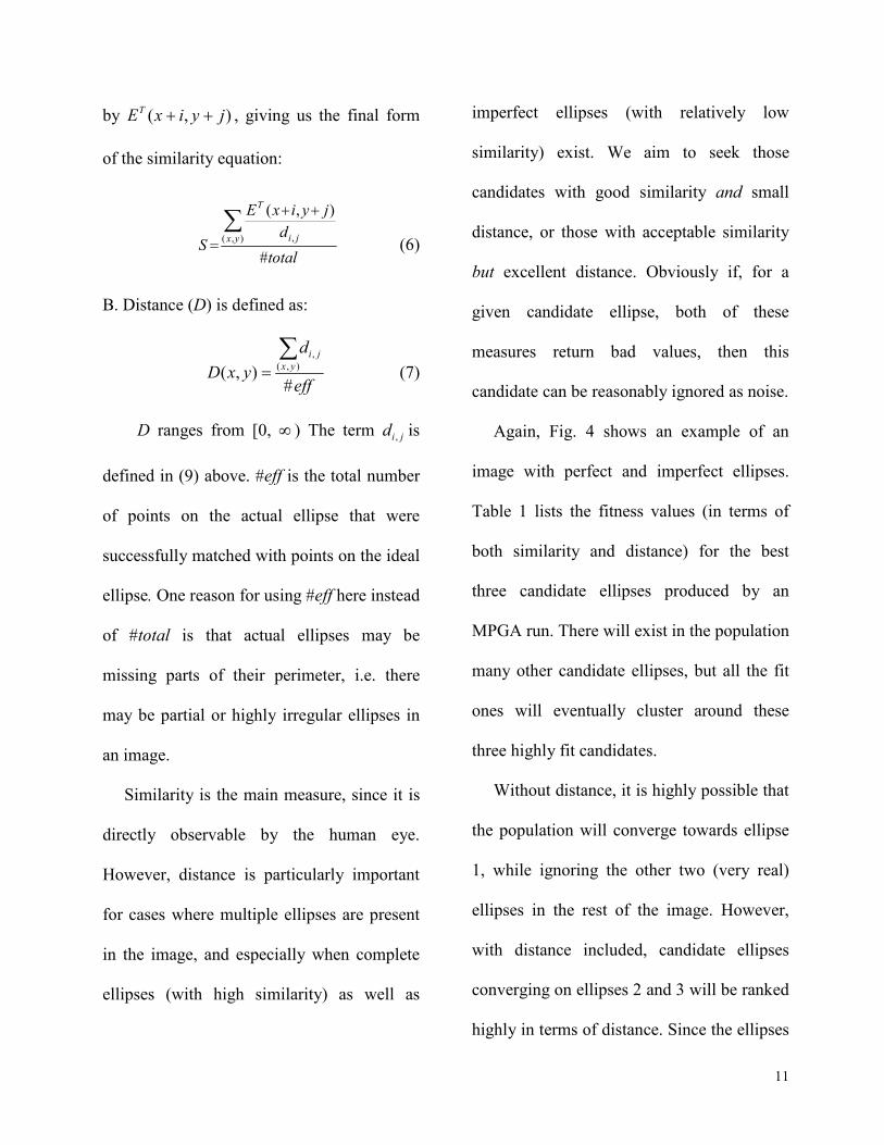
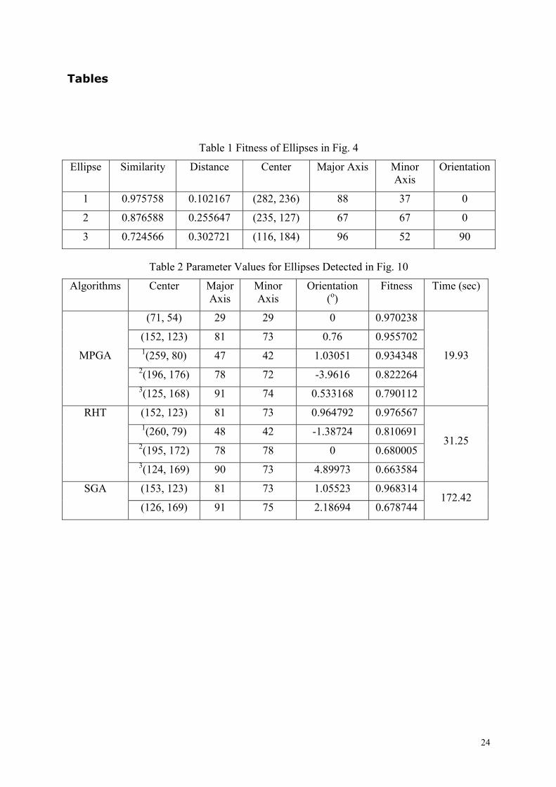
Again, Fig. 4 shows an example of an

image with perfect and imperfect ellipses.

Table 1 lists the fitness values (in terms of

both similarity and distance) for the best

three candidate ellipses produced by an

MPGA run. There will exist in the population

many other candidate ellipses, but all the fit

ones will eventually cluster around these

three highly fit candidates.

Without distance, it is highly possible that

the population will converge towards ellipse

1, while ignoring the other two (very real)

ellipses in the rest of the image. However,

with distance included, candidate ellipses

converging on ellipses 2 and 3 will be ranked

highly in terms of distance. Since the ellipses

11

converging towards these two ellipses will

have acceptable similarity but excellent

distance, this will result in a reasonable

clustering (and hence subdivision) of the

population, instead of complete domination

by ellipse 1 candidates.

In MPGA, fitness is computed in the

following manner: the 10 numbers of each

chromosome are substituted in 5

simultaneous ellipse equations. If the

equations fail to produce a solution then this

chromosome does not represent any kind of

ellipse. Hence, this chromosome is assigned

the minimum fitness of 0. If the equations

produce a solution, then equations (6 and 7)

are used to compute the similarity and

distance of this chromosome. These two

values together represent the fitness of the

evaluated chromosome.

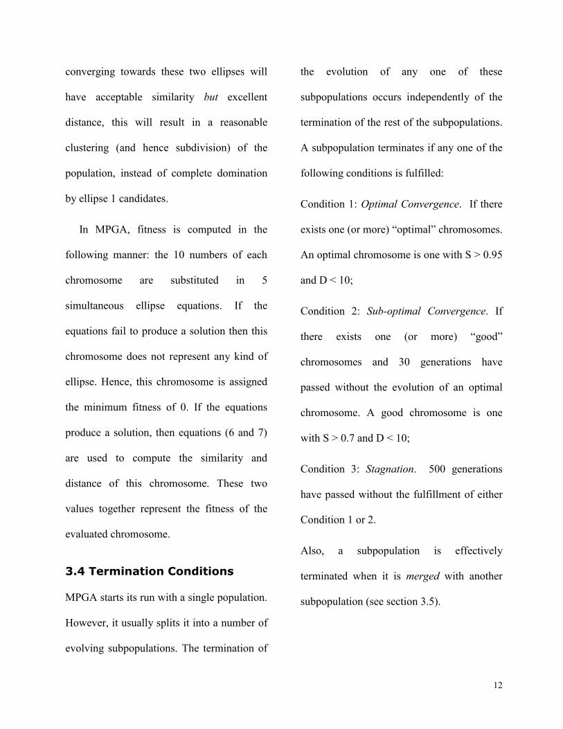
3.4 Termination Conditions

MPGA starts its run with a single population.

However, it usually splits it into a number of

evolving subpopulations. The termination of

the evolution of any one of these

subpopulations occurs independently of the

termination of the rest of the subpopulations.

A subpopulation terminates if any one of the

following conditions is fulfilled:

Condition 1: Optimal Convergence. If there

exists one (or more) “optimal” chromosomes.

An optimal chromosome is one with S > 0.95

and D < 10;

Condition 2: Sub-optimal Convergence. If

there exists one (or more) “good”

chromosomes and 30 generations have

passed without the evolution of an optimal

chromosome. A good chromosome is one

with S > 0.7 and D < 10;

Condition 3: Stagnation. 500 generations

have passed without the fulfillment of either

Condition 1 or 2.

Also, a subpopulation is effectively

terminated when it is merged with another

subpopulation (see section 3.5).

12

3.5 Clustering: Migration,

Splitting and Merging

A subpopulation is called a cluster. The

centre of a cluster is the chromosome with

the greatest similarity. If more than one

exists then the one with the least distance is

declared the centre.

In the MPGA algorithm, the algorithm

starts with a single population (or cluster) in

which individuals are ranked in terms of both

similarity and distance. The initial single

population, and later subpopulations, are

manipulated through a clustering process.

This process involves Migration, Splitting

and Merger (explained below).

In each subpopulation, all good

chromosomes (S>0.7 and D<10) are either

kept in their own cluster or placed into a

different existing or newly-created cluster.

All not-good chromosomes are simply left in

their own cluster (and are eventually

eliminated be selection- see section 3.6).

The Euclidean distance ED between a

good chromosome and the various existing

cluster centers determines whether this

chromosomes remains in its own cluster or

moves. ED is computed as follows: given

two sets of ellipse parameters (a1, b1, x1, y1,

ω1) and (a2, b2, x2, y2, ω2):

5)()()()()( 2

212

212

212

212

21 �� ���������

�

yyxxbbaaED (8)

(ai, bi) is the long and short axis, (xi, yi) is

the center and ωi is the orientation. When a

chromosome migrates from subpopulation A

to subpopulation B, it replaces the weakest

chromosome in the latter, and the vacancy in

the former is filled by the processes of

evolution (see section 3.6).

A. Migration. If the Euclidean distance

between a chromosome and its own cluster

centre is lower than a pre-defined threshold

t1 then this chromosome is moved to another

cluster. To determine which one, the ED

between this chromosome and every other

cluster center is measured. If one or more

cluster centers is closer to it than t1 then the

13

chromosome moves (migrates) to the cluster

with the closest centre to it.

B. Splitting. If the algorithm is unable to find

a cluster (with a centre) sufficiently close to a

migrating chromosome, then a new cluster is

created around this chromosome. This action

is called splitting.

C. Mergeing. An empirically-derived

threshold � is used to define the minimum

allowable Euclidean distance between any

two different cluster centers. As two different

clusters may evolve toward a single (local or

global optimum), any two clusters with

centers closer to each other than � are

merged. This is done by taking the fittest

50% (in terms of similarity) of the

chromosomes in each cluster and placing

them in the new merged cluster. This action

is called merging.

d

d

All clusters are checked periodically

(every 30 generations), to see whether some

of them could be merged. Merging is barred

for the first 50 generations, and (as stated) is

only possible after each periodic check. This

is so because early or/and frequent mergers

would greatly reduce the diversity of the

whole population.

Hence, through the three processes of

migration, splitting and merger, clustering

works to maintain a number of

subpopulations that are independently

evolved towards local and global optima.

Evolution is explained in the next section.

3.6 Evolution: Selection and

Diversification

Evolution proceeds mainly via Selection and

Diversification. Selection eliminates those

chromosomes in the population that are not

very fit, focusing the search on promising

areas of the fitness surface. On the other

hand, diversity is achieved via crossover and

mutation, which together serve to direct the

search towards new and potentially

promising areas. In MPGA, selection is

realized using Elitism and Fitness

14

Proportional Selection. Diversification is

realized via Crossover and Mutation.

During evolution of a subpopulation,

elitism copies the fittest 15% of the current

generation (by similarity) into the next

generation, without modification. Following

that, two chromosomes are selected from the

whole current population. The probability of

selecting a chromosome is proportional to its

relative fitness (similarity). The two

chromosomes are crossed-over, with

probability 0.6. The result, whether it is two

new chromosomes or the original parent

chromosomes, are mutated (on a bit-wise

basis) with probability 0.1. This process of

selection and crossover-mutation continues

until the next generation is complete. As

stated, we use constant size subpopulations

of between 30 and 100 chromosomes.

Finally, every new chromosome

introduced into the next generation is tested

to see if it is a good chromosome or not

(S>0.7, D< 10); if it is not then it is left in the

same subpopulation. If however it proves to

be a good chromosome then it is tested for

migration-splitting, and is then either kept in

its current subpopulation or moved to another

existing or new subpopulation (see section

3.5).

In MPGA, Crossover and Mutation are

special operations designed specifically for

shape detection applications. We describe

them in detail below, starting with crossover.

Given the fact that (a) the overall

population is divided into a number of

subpopulations, each effectively clustering

around an ellipse in the image; and (b) each

chromosome is defined by a set of points on

the perimeter of an ellipse, we can assert that

simple single point crossover is an effective

method of crossover for our application. A

pivot is selected at random, and the parent

chromosomes’ genes on either side of the

pivot are swapped to create the offspring. See

Fig. 7.

The effect of the crossover operation, on

the actual ellipses represented by the

chromosomes, is shown in Fig. 8.

15

For mutation, we define a new mutation

operator, configured specifically for our

application. First a gene (or point) is

randomly selected from the chromosome that

we intend to mutate. As shown in Fig. 8, this

point acts as the starting point for a path (r)

that traverses the perimeter of a pattern, until

a (pre-set) maximum number of points is

traversed, or an end- or intersection point is

reached. If r > 10, the remaining genes

(points) are also picked, at random, from this

path. As long as the starting point lies on a

promising candidate ellipse, it is highly

possible that the other points will do so as

well. This method of mutation greatly

enhances the possibility of mutating a given

chromosome into a better one.

Fig. 9 illustrates the mutation process.

The original genes are P1, P2, P3, P4, and P5.

The starting point, P1 is selected and path r is

traversed. The other new genes, Q2, Q3, Q4,

and Q5 are randomly selected from path r,

and copied into the mutated chromosome.

Hence, the new chromosome becomes

(P1Q2Q3Q4Q5).

Hence, evolution hand-in-hand with

clustering (which mainly precedes but also

acts during evolution) direct the various

subpopulations to local and global optima

centered on the various ellipses in the target

image.

4. Experimental Results and

Analysis

This section compares the performance of the

MPGA, SGA and RHT algorithms, using

synthetic and real-world images. To carry out

a fair comparison between these three

different algorithms, we use (a) the same

method for computing fitness, in terms of

similarity and distance (described in section

3.4), and (b) the same numerical technique

for computing the geometric parameters of

an ellipse (see section 3.1). This neutralizes

any advantages that may be gained via using

more efficient methods, which reduce

16

dimensionality or utilize symmetry [5, 7, 9,

13].

All our experiments were run on an Intel

Xeon 2.66 GHz w/ 512 KB of cache, 512

MB DDR RAM and running Red Hat Linux

8.0.3.2-7.

We have two main categories of test data,

which are synthetic images and real world

images. Accuracy here, is defined as the

ratio of correctly detected ellipses, in relation

to the total number of ellipses actually

present in the target image. If over detection

occurs, then that is reflected in the false

positive statistics.

4.1 Synthetic Images

The synthetic images are comprised of two

sets, set A and set B. Set A is partitioned

into 7 collections of 50 images each (totaling

350 images). These collections are used to

test the algorithms’ performance on images

with different numbers of ellipses. Hence, the

first collection contains 50 images of single

ellipses, the second collection contains

images of two ellipses, and so on. The final

collection contains 50 images of 7 ellipses.

Set B, on the other hand, is used to test the

algorithms’ performance on noisy images.

Hence, this set is made of 5 collections of 50

images each (totaling 250 images). The first,

second, third, fourth and fifth collections

contain images with 0%, 0.5%, 1%, 3% and

5% salt-and-pepper noise, respectively.

The ellipses in the synthetic image

database are not all full and perfectly formed

ellipses; we make sure that some images in

both sets have at least 1 partial or deformed

ellipse. A typical example is presented in

Fig. 10 (with numerical results presented in

Table 2). In this figure there are 5 ellipses, 2

of which are malformed. The figure also

shows the results, in terms of detected

ellipses, of applying MPGA, RHT and SGA

to this image.

As seen in Fig. 10 (b), RHT misses the

smallest ellipse since the probability of

locating it is smaller than the probability of

locating the other larger ellipses. The fitness

17

values shown in Table 2 are those of

similarity and not distance (or some

combination of the two) because: (a)

similarity is the only measure/factor of

fitness used by all these three algorithms, and

(b) similarity is more intuitive than any

combination of measures, since it closely

corresponds the human conception of

similarity between shapes.

In reference to Table 2, MPGA returns

better fitness values than RHT, for ellipses 1,

2 and 3. This is because MPGA, via

evolution, executes an iterative and parallel

search, focused at different localities of the

of the search space, while the RHT carries

out a one-shot blind search through the

whole space.

Fig. 11 contrasts the performance of the

three algorithms in terms of accuracy as well

as average CPU running time. Fig. 11(a)

shows that the accuracy of SGA decreases

dramatically as the number of ellipses

increase. Similarly, the accuracy of RHT also

decreases gradually from 100% for one

ellipse to approximately 80% for seven

ellipses. In contrast, MPGA outperforms the

other two algorithms by maintaining an

almost perfect level of detection accuracy,

and slightly dipping to around 98%, for

images with seven ellipses.

Fig. 11(b) demonstrates the clear

advantage that MPGA has over both RHT

and GAS in regards to speed time. It graphs

the amount of CPU time utilized (on

average) by the various algorithms for the

detection of images with 1-7 ellipses. There

is almost no difference in speed for images

with 4 or less ellipses. However, for 5 or

more ellipses, MPGA realizes a clear and

widening gap in speed.

Fig. 12(a) shows a typical image with 5%

pepper-and-salt noise. Ellipses detected by

MPGA are shown in Fig. 12(b)

Generally, RHT is more liable to false

positives (i.e. the detection of non-existing

ellipses). Fig. 12(c) demonstrates that. Table

3 presents the exact numerical results.

18

Fig. 13 shows the performance of these

algorithms on noisy images. Again, MPGA

shows considerable robustness in the

presence of salt-and-pepper noise, while

simultaneously operating faster than the

other two algorithms.

Many false positives are observed for

RHT with high noise, as Fig. 14 shows. This

fact further fortifies our claim (in section 1)

that RHT searches the space and accumulates

votes blindly. Therefore non-existing ellipses

may get enough votes in highly noisy

images, as is the case in Fig. 14.

4.2 Real World Images

Large, carefully constructed databases of

synthetic images (600, in our case) provide

the bases for comprehensive tests, which also

provide specific feedback about potential

problems with detection algorithms.

Nevertheless, it is real-world images that

determine the difference between a genuinely

useful and purely academic novel algorithm.

Hence, we have amassed three databases of

intentionally different types of images: hand-

written English letters, microscopic cell

images and road signs. The databases are of

varying size, but contain images that were

collected, prior to even the design of MPGA.

From each of those databases, 50 images, are

selected at random, and then used for the

purpose of assessing the real-world

performance of MPGA, RHA and SGA. On

visual inspection, we noticed that these

images contain: all kinds of combinations of

perfect and deformed ellipses, noise levels,

and other geometric shapes (e.g. lines).

Fig. 15(a) shows a typical handwritten

character with elliptical curves detected.

In Table 4 we can see that MPGA is

slower than RHT. As discussed in section 1,

when the image is relatively simple and

noise-free and does not have many

overlapping patterns, RHT is expected to run

faster than MPGA. However, RHT still

suffers from false positives, as Fig. 15(c)

shows, and generally, in pattern recognition,

19

accuracy of detection is of a higher priority

than speed of processing.

Fig. 16(a) is a typical microscopic image

of cells. Here, MPGA shows its obvious

advantage over RHT and SGA in both

accuracy and speed. Although RHT

approximates all eight cells, it suffers from

large misplacement (see cells labeled: a, b, c

and d, in Fig. 16(d)) and long running times;

SGA fails to detect even a single ellipse.

Table 5 contains the exact numerical results.

Fig. 17 is a typical image of a road sign.

We can see that neither RHT nor SGA is able

to detect partial ellipses, especially when

there are also perfect ellipses in the image.

They are generally slower than MPGA in this

kind of complicated images. Table 6 presents

the exact numerical results.

Table 7 gives out the overall performance

for real world images. From the table we can

see that SGA is almost totally ineffective

with complicated real world images; it

returns an average accuracy of less than 20%.

RHT suffers from long computation times

and high false positive rate.

There are some false positives (6.9048%)

for MPGA as well, because for some

polygons, the algorithm may sometimes

approximate them with ellipses. One possible

solution is to detect low dimensional shapes

first (such as lines), and remove these from

the image, before detecting circles and

ellipses. This way, the process can be both

made more efficient and more accurate.

5. Conclusions and Future Work

This paper presents a new GA, one which

uses (a) multiple-populations and an

elaborate process of evolution-clustering to

(b) efficiently and accurately detect (c)

multiple potentially-deformed full and partial

ellipses in noisy images. This algorithm, was

thoroughly tested on a large number of

synthetic and three types of real-world

images, and compared to the very widely-

used RHT and one of the best-available GA-

based ellipse detection technique: SGA.

20

Despite the conceptual complexity of the

MPGA algorithm, the program implementing

the new algorithm performed, generally

speaking, more efficiently and more

accurately than both RHT and SGA.

However, this does not mean that there is no

room for improvements.

We intend to improve the MPGA by

getting to:

1. Detect (and remove) lines and polygons,

first, so that any complicated images can be

analyzed within a reasonable period of time;

2. Run without the need for prior tuning of

GA parameters, such as mutation and

crossover probabilities. This can be done by

incorporating the ideas of Parameterless

GAs, which we have already experimented

with, successfully, but only tested using

mathematically-defined fitness surfaces.

References

[1] D.H. Ballard, “Generalizing the Hough

Transform to Detect Arbitrary Shapes”,

Pattern Recognition, Vol. 13, No. 2, 1981,

pp. 111-122

[2] Samarjit Chakraborty and Kalyanmoy

Deb, “Analytic Curve Detection from a

Noisy Binary Edge Map Using Genetic

Algorithm”, PPSN, 1998, pp. 129-138

[3] D. E. Goldberg and J. Richardson,

"Genetic algorithms with sharing for

multimodal function optimization,"

Proceeding of the 2nd Int. Conference on

Genetic Algorithms, J. J. Grefenstette, Ed.

Hillsdale, NJ: Lawrence Erlbaum, 1987, pp.

41-49

[4] W. E. L. Grimson and D. P. Huttenlocher,

“On the sensitivity of the Hough transform

for object recognition”, IEEE Trans. Pattern

Anal. Machine Intelli., Vol. 12, No. 3, March

1990, pp. 255-274

[5] N. Guil and E. L. Zapata, “Lower order

circle and ellipse Hough Transform”, Pattern

Recognition, Vol.30, No.10, 1997, pp.1729-

1744

21

[6] Hearn and M. P. Baker, Computer

Graphics C Version, D., Prentice Hall, Inc.,

1997.

[7] Chun-TA HO and Ling-Hwei Chen, “A

Fast Ellipse/Circle Detector Using Geometric

Symmetry”, Pattern Recognition, Vol. 28,

No.1, 1995, pp. 117-124

[8] P.V.C. Hough, “Machine Analysis of

Bubble Chamber Pictures”, International

Conference on High Energy Accelerators and

Instrumentation, CERN, 1959

[9] Yiwu Lei, Kok Cheong Wong, “Ellipse

detection based on symmetry”, Pattern

Recognition Letters, Vol. 20, No. 1, January

1999, pp. 41-47

[10] Evelyne Lutton and Patrice Martinez,

“A Genetic Algorithm for the Detection of

2D Geometric Primitives in Images”,

Proceedings of the 12th International

Conference on Pattern Recognition,

Jerusalem, Israel, 9-13 October 1994, Vol. 1,

pp. 526-528

[11] Tomas Mainzer, “Genetic Algorithm for

traffic sign detection”, Applied Electronic

2002

[12] Tomas Mainzer, “Genetic Algorithm for

Shape Detection”, Technical Report no.

DCSE/TR-2002-06, University of West

Bohemia, 2002

[13] Robert A. McLaughlin, “Randomized

Hough Transform: Improved ellipse

detection with comparison”, Pattern

Recognition Letters, Vol. 19, No. 3-4, March

1998, pp. 299–305

[14] S Procter and J Illingworth, “A

Comparison of the Randomized Hough

Transform and a Genetic Algorithm for

Ellipse Detection”, Pattern Recognition in

Practice IV: multiple paradigms, comparative

studies and hybrid systems, edited by E

Gelsema and L Kanal, Elsevier Science Ltd.,

pp. 449-460

[15] G. Roth and M. D. Levine. “Geometric

primitive extraction using a genetic

algorithm”, IEEE Transactions on Pattern

22

Analysis and Machine Intelligence, Vol. 16,

No. 9, September 1994, pp. 901-905

[16] R. E. Smith, S. Forrest and A. S.

Perelson, “Searching for diverse, cooperative

populations with genetic algorithms”, TCGA

Report No. 92002, The University of

Alabama, Dept. of Engineering Mechanics,

1992.

[17] William H. Press et Al., Numerical

Recipes in C, The Art of Scientific

Computing Second Edition, Cambridge

University Press, 1992, Chapter 2, pp. 43-50

[18] Lei Xu, E.Oja, & P.Kultanen, “A New

Curve Detection Method: Randomized

Hough Transform (RHT)”, Pattern

Recognition Letters, Vol. 11, No. 5, May

1990, pp. 331-338

23

Tables

Table 1 Fitness of Ellipses in Fig. 4

Ellipse Similarity Distance Center Major Axis Minor Axis

Orientation

1 0.975758 0.102167 (282, 236) 88 37 0

2 0.876588 0.255647 (235, 127) 67 67 0

3 0.724566 0.302721 (116, 184) 96 52 90

Table 2 Parameter Values for Ellipses Detected in Fig. 10

Algorithms Center Major Axis

Minor Axis

Orientation (o)

Fitness Time (sec)

(71, 54) 29 29 0 0.970238

(152, 123) 81 73 0.76 0.955702 1(259, 80) 47 42 1.03051 0.934348

2(196, 176) 78 72 -3.9616 0.822264

MPGA

3(125, 168) 91 74 0.533168 0.790112

19.93

(152, 123) 81 73 0.964792 0.976567 1(260, 79) 48 42 -1.38724 0.810691

2(195, 172) 78 78 0 0.680005

RHT

3(124, 169) 90 73 4.89973 0.663584

31.25

(153, 123) 81 73 1.05523 0.968314 SGA

(126, 169) 91 75 2.18694 0.678744 172.42

24

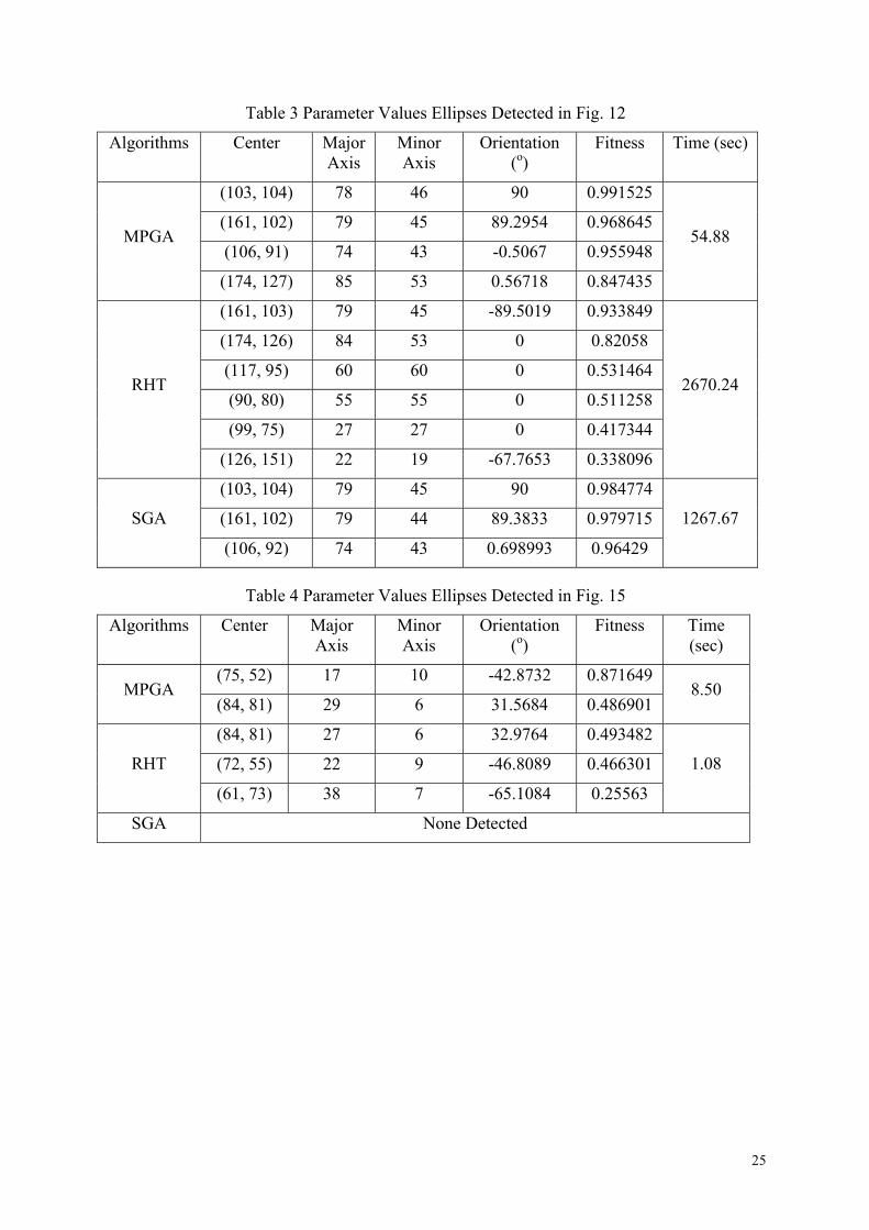
Table 3 Parameter Values Ellipses Detected in Fig. 12

Algorithms Center Major Axis

Minor Axis

Orientation (o)

Fitness Time (sec)

(103, 104) 78 46 90 0.991525

(161, 102) 79 45 89.2954 0.968645

(106, 91) 74 43 -0.5067 0.955948 MPGA

(174, 127) 85 53 0.56718 0.847435

54.88

(161, 103) 79 45 -89.5019 0.933849

(174, 126) 84 53 0 0.82058

(117, 95) 60 60 0 0.531464

(90, 80) 55 55 0 0.511258

(99, 75) 27 27 0 0.417344

RHT

(126, 151) 22 19 -67.7653 0.338096

2670.24

(103, 104) 79 45 90 0.984774

(161, 102) 79 44 89.3833 0.979715 SGA

(106, 92) 74 43 0.698993 0.96429

1267.67

Table 4 Parameter Values Ellipses Detected in Fig. 15

Algorithms Center Major Axis

Minor Axis

Orientation (o)

Fitness Time (sec)

(75, 52) 17 10 -42.8732 0.871649 MPGA

(84, 81) 29 6 31.5684 0.486901 8.50

(84, 81) 27 6 32.9764 0.493482

(72, 55) 22 9 -46.8089 0.466301 RHT

(61, 73) 38 7 -65.1084 0.25563

1.08

SGA None Detected

25

Table 5 Parameter Values Ellipses Detected in Fig. 16

Algorithms Center Major Axis

Minor Axis

Orientation (o)

Fitness Time (sec)

(70, 110) 24 12 78.7455 0.884863

(41, 57) 23 18 -26.4053 0.871432

(111, 101) 20 14 -19.6434 0.855267

(272, 112) 22 16 82.1506 0.844027

(48, 133) 27 16 -89.4256 0.841953

(242, 63) 27 15 -33.6307 0.837715

(144, 23) 20 14 26.6459 0.734521

MPGA

(107, 53) 24 11 22.4682 0.649748

26.71

(47, 133) 25 17 87.6509 0.747763

(38, 58) 20 20 0 0.644028

(70, 112) 25 13 78.18 0.74799

(243, 63) 27 16 33.7181 0.805789

(89, 48) 44 12 18.0898 0.34089

(147, 24) 17 14 34.4332 0.639102

(106, 101) 26 14 -14.8053 0.478279

RHT

(271, 113) 19 16 48.1021 0.627391

1015.98

SGA None Detected

Table 6 Parameter Values Ellipses Detected in Fig. 17

Algorithms Center Major Axis

Minor Axis

Orientation (o)

Fitness Time (sec)

(224, 200) 188 188 0 0.993062

(223, 200) 157 157 0 0.908382

(255, 160) 39 36 9.34395 0.654582 MPGA

(264, 161) 79 79 0 0.401485

140.68

(224, 200) 188 188 0 0.993062 RHT

(223, 201) 158 156 0 0.908279 335.08

(224, 200) 188 188 0 0.993062 SGA

(222, 200) 157 157 0 0.886644 378.74

26

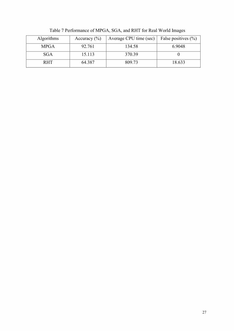
Table 7 Performance of MPGA, SGA, and RHT for Real World Images

Algorithms Accuracy (%) Average CPU time (sec) False positives (%)

MPGA 92.761 134.58 6.9048

SGA 15.113 370.39 0

RHT 64.387 809.73 18.633

27

Figures

(a) (b)

Fig. 1 Global and Local Optima (a) a Large Imperfect Ellipse (Left) and a much Smaller Perfect Ellipse (Right)

(b) Locally-Optimum Candidate Ellipse Overlaid on top of Left Ellipse

Clusterin

Evolution

Evaluate Fitness (rank) & Select

Convergence N

End

Initialize First

Y

Fig. 2 Summary Flow Chart of MPGA Algorithm

Fig. 3 The Geometric Parameters of an Ellipse

28

Fig. 4 Perfect and Imperfect Ellipses

Fig. 5 Matching of a Candidate Ellipse, Point by Point, to Potential Actual Ellipses in an Image

Fig. 6 2D Geometric Transformation of Ellipse

Fig. 7 Result of Crossing-Over Two Chromosomes: Genotypic View

29

Fig. 8 Result of Crossing-Over Two Chromosomes: Phenotypic View

Fig. 9 Mutation Operation

(a) (b)

(c) (d)

Fig. 10 A Typical Image with Multiple Ellipses: Detected Ellipses Overlaid in Thick Grey Line

(a) Original Image (b) Ellipses Detected by MPGA (c) Ellipses Detected by RHT (d) Ellipses Detected by SGA

30

(a) (b)

Fig. 11 Comparing the Performance of RHT, SGA and MPGA when Detecting Multiple Ellipses in an Image

(a) Accuracy vs. Number of Ellipses (b) CPU Time vs. Number of Ellipses

(a) (b)

(c) (d)

Fig. 12 A Typical Noisy Image with %5 Salt & Pepper Noise: Detected Ellipses Overlaid in Thick Grey Line

(a) Original Image (b) Ellipses Detected by MPGA (c) Ellipses Detected by RHT (d) Ellipses Detected by SGA

31

Fig. 13 Comparing the Performance of RHT, SGA and MPGA when Detecting Ellipses in Noisy Images

(a) Accuracy vs. Ratio of Noise in Image (b) CPU Time vs. Ratio of Noise in Image

Fig. 14 False positives for different noise level

(a) (b) (c)

Fig. 15 A Typical Handwritten Character (Capital R): Detected Ellipses Overlaid in Thick Grey Line - SGA Failed to Detect a Single Ellipse

(a) Original Image (b) Ellipses Detected by MPGA (c) Ellipses Detected by RHT

32

(a) (b)

(c) (d)

Fig. 16 A Typical Image of Cells taken through a Microscope (at 40x) - SGA Failed to Detect a Single Ellipse

(a) Original Image (b) Pre-processed Image (c) Ellipses Detected by MPGA (d) Ellipses Detected by RHT

(a) (b)

(c) (d & e)

Fig. 17 Typical Road sign Image (a) Original Image (b) Pre-processed Image (c) Ellipses Detected by MPGA (d) Ellipses

Detected by RHT (e) Ellipses Detected by SGA

33