robust control of time-delay systems - illinois...
TRANSCRIPT

Robust Control of Time-delaySystems
Qing-Chang Zhong
Distinguished Lecturer, IEEE Power Electronics SocietyMax McGraw Endowed Chair Professor in Energy and Power Engineering
Dept. of Electrical and Computer EngineeringIllinois Institute of Technology
Email: [email protected]
Web: http://mypages.iit.edu/∼qzhong2/
Qing-Chang Zhong (IIT, Chicago, [email protected]) Robust Control of Time-delay Systems

Outline
Notations and some preliminaries
Standard H∞ control problem
Delay-type Nehari problem
Controller implementation
Qing-Chang Zhong (IIT, Chicago, [email protected]) Robust Control of Time-delay Systems

Notations
Given a matrix A, AT and A∗ denote its transposeand complex conjugate transpose respectively. A−∗
stands for (A−1)∗ when the inverse A−1 exists.
G (s) = D + C (sI − A)−1B.=
[
A B
C D
]
G∼(s) = [G (−s∗)]∗ =
[
−A∗ −C ∗
B∗ D∗
]
Fl and Fu are the commonly-used lower/upper linearfractional transformation (LFT).
Qing-Chang Zhong (IIT, Chicago, [email protected]) Robust Control of Time-delay Systems
Preliminaries
Two operators
Chain-scattering representation
Homographic transformation
Qing-Chang Zhong (IIT, Chicago, [email protected]) Robust Control of Time-delay Systems

Completion operator
A completion operator πh is defined for h ≥ 0 as:
πh{G}.=
[
A B
Ce−Ah 0
]
−e−sh
[
A B
C D
]
.= G (s)−e−shG (s).
0 0.2 0.4 0.6 0.8 h=1 1.2 1.40
1
2
3
4
Time (sec)
Impu
lse
resp
onse
G
πh(G)
e−shG
shift
Qing-Chang Zhong (IIT, Chicago, [email protected]) Robust Control of Time-delay Systems

Truncation operator
A truncation operator τh is defined for h ≥ 0 as:
τh{G}.=
[
A B
C D
]
− e−sh
[
A eAhB
C 0
]
.= G (s)− e−shG (s)
0 0.2 0.4 0.6 0.8 h=1 1.2 1.40
1
2
3
4
Time (sec)
Impu
lse
resp
onse
G
τh(G)
Qing-Chang Zhong (IIT, Chicago, [email protected]) Robust Control of Time-delay Systems

Representations of systems
Input-output rep.
Cl(M)
(a) the left CSR
Cr(M)
(b) the right CSR
Chain-scattering rep.Qing-Chang Zhong (IIT, Chicago, [email protected]) Robust Control of Time-delay Systems

Chain-scattering representation
For M =
[
M11 M12
M21 M22
]
, the right and left
chain-scattering representations are defined as:
Cr(M).=
[
M12 −M11M−121 M22 M11M
−121
−M−121 M22 M−1
21
]
Cl(M).=
[
M−112 −M−1
12 M11
M22M−112 M12 −M22M
−112 M11
]
provided that M21 and M12, respectively, areinvertible. If both M21 and M12 are invertible, then
Cr (M) · Cl(M) = I .
Qing-Chang Zhong (IIT, Chicago, [email protected]) Robust Control of Time-delay Systems
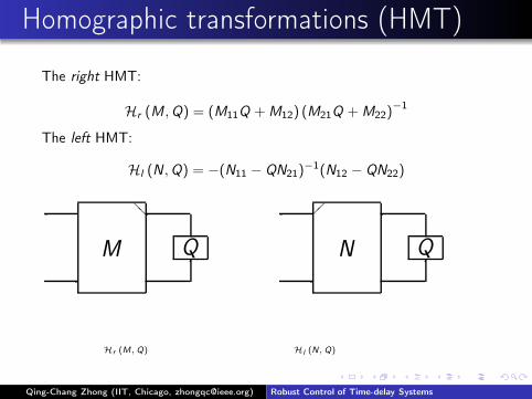
Homographic transformations (HMT)
The right HMT:
Hr (M ,Q) = (M11Q +M12) (M21Q +M22)−1
The left HMT:
Hl (N ,Q) = −(N11 − QN21)−1(N12 − QN22)
M
❅❅
Q
✲
✛ ✛
✻
N
��
Q
✲
✛ ✛
✻
Hr (M,Q) Hl (N,Q)
Qing-Chang Zhong (IIT, Chicago, [email protected]) Robust Control of Time-delay Systems

Properties of the HMT
Lemma
Hr satisfies the following properties:(i) Hr(Cr(M), S) = Fl(M , S);(ii) Hr (I , S) = S ;(iii) Hr (M1,Hr(M2, S) = Hr(M1M2, S);(iv) If Hr(G , S) = R and G−1 exists, then
S = Hr (G−1,R).
Lemma
Let Λ be any unimodular matrix, then the H∞
control problem ‖Hr(G , K0)‖∞ < γ is solvable iff‖Hr(GΛ, K )‖∞ < γ is solvable. Furthermore,K0 = Hr(Λ, K ) or K = Hr(Λ
−1, K0).Qing-Chang Zhong (IIT, Chicago, [email protected]) Robust Control of Time-delay Systems

Outline
Notations and some preliminaries
Standard H∞ control problem
Delay-type Nehari problem
Controller implementation
Qing-Chang Zhong (IIT, Chicago, [email protected]) Robust Control of Time-delay Systems

Standard H∞ problem of single-delay systems
Given a γ > 0, find a proper controller K such thatthe closed-loop system is internally stable and
∥
∥Fl(P, Ke−sh)∥
∥
∞< γ.
P
e−shI
K
✛
✛ ✛
✛
y
z
u
w
u1
✲
Qing-Chang Zhong (IIT, Chicago, [email protected]) Robust Control of Time-delay Systems

Key steps to solve the SPh
The SPh is solved via solving two simpler problems:
The one-block problem (OPh): in the form of SPh butwith P(∞) =
[
0 I
I 0
]
.
An extended Nehari problem (ENPh): in the form ofNPh but minimising the H∞-norm of Gβ11 + e−shQβ.
Key steps:
Step 1: reduce SPh to SP0 + OPh
Step 2: reduce OPh to ENPh
Step 3: solve ENPh
Step 4: recover the controllers
Qing-Chang Zhong (IIT, Chicago, [email protected]) Robust Control of Time-delay Systems

Reducing SPh to SP0 + OPh
Cr(P)
❅❅ e−shI
K
✲
✛ ✛ ✛
w
z u
y
u1
✻
Cr (P)
❅❅
Gα
❅❅
Cr(Gβ)
❅❅ e−shI
K
Delay-free problem 1-block delay problem
✲
✛
✲
✛
✲
✛ ✛ ✛
w
z u
y
u1
✻
w1
z1
y
u1
Gα is the controller generator of SP0. Gβ is defined such that Cr (Gβ ).= G−1
α . Gα and Cr (Gβ ) are allbistable.
Qing-Chang Zhong (IIT, Chicago, [email protected]) Robust Control of Time-delay Systems

Reducing OPh to ENPh (I)
Qα(s) = Hr (Cr (Gβ ), e−shK ) = Fl (Gβ, e−shK )
= Gβ11 + Gβ12Ke−sh(I − Gβ22Ke
−sh)−1Gβ21
❤
Gβ11
Gβ12
Gβ22
Gβ21❤
∆2
e−shI
❤
Kh(s)
✛
✲
+
-
K (s)✛
✲ ✲
✛✛
✻
✻
✻
❄
❄
❄
❄
z1
w1
u1
y
u
Introducing a Smith predictor
∆2(s) = −πh{Gβ22}.= −Gβ22 + e−shGβ22
Qing-Chang Zhong (IIT, Chicago, [email protected]) Robust Control of Time-delay Systems

Reducing OPh to ENPh (II)
❤
Gβ11
Gβ12e−shI
Gβ21
Gβ22
❤
Kh(s)
✛
✲
+Qβ(s)✛
✲
✛✛
✻
✻
✻
❄
❄
z1
w1
u2
z2
Qβ.= Hr (
[
Gβ12 0
−G−1β21Gβ22(s) G−1
β21
]
,Kh)
The OPh is now reduced to ENPh:‖Qα(s)‖∞ =
∥
∥Gβ11 + e−shQβ
∥
∥
∞< γ.
Qing-Chang Zhong (IIT, Chicago, [email protected]) Robust Control of Time-delay Systems

Solution to the SPh
Solvability ⇐⇒ :
H0 ∈ dom(Ric) and X = Ric(H0) ≥ 0;
J0 ∈ dom(Ric) and Y = Ric(J0) ≥ 0;
ρ(XY ) < γ2;
γ > γh, where γh = max{γ : detΣ22 = 0}.
Z V−1
❤
Q
❅❅
✲-
u
y✲
✛✛
✻
❄
❄
V−1 =
A+ B2C1 B2 − Σ12Σ−122 C
∗1 Σ−∗
22 B1
C1 I 0−γ−2B∗
1Σ∗21 − C2Σ
∗22 0 I
Qing-Chang Zhong (IIT, Chicago, [email protected]) Robust Control of Time-delay Systems

Outline
Notations and some preliminaries
Standard H∞ control problem
Delay-type Nehari problem
Controller implementation
Qing-Chang Zhong (IIT, Chicago, [email protected]) Robust Control of Time-delay Systems

The delay-type Nehari problem
Given a minimal state-space realisation Gβ =[
A B
−C 0
]
,
which is not necessarily stable, and h ≥ 0,characterise the optimal value
γopt = inf{∥
∥Gβ(s) + e−shK (s)∥
∥
L∞: K (s) ∈ H∞}
and for a given γ > γopt , parametrise the suboptimalset of proper K ∈ H∞ such that
∥
∥Gβ(s) + e−shK (s)∥
∥
L∞< γ.
Qing-Chang Zhong (IIT, Chicago, [email protected]) Robust Control of Time-delay Systems

The optimal value
It is well known that this problem is solvable iff
γ > γopt.=
∥
∥ΓeshGβ
∥
∥ , (1)
where Γ denotes the Hankel operator. The symboleshGβ is non-causal and, possibly, unstable.
The problem is how to characterise it.
Qing-Chang Zhong (IIT, Chicago, [email protected]) Robust Control of Time-delay Systems

Estimation of γopt
It is easy to see that
γopt ≤ ‖Gβ(s)‖L∞
because at least K can be chosen as 0. It can be seen from(1) that γopt ≥
∥
∥ΓGβ
∥
∥. Hence,
∥
∥ΓGβ
∥
∥ ≤ γopt ≤ ‖Gβ(s)‖L∞ . (2)
When γ ≤ ‖Gβ(s)‖L∞ , the matrix
H =
[
A γ−2BB∗
−C ∗C −A∗
]
has at least one pair of eigenvalues on the jω-axis.
Qing-Chang Zhong (IIT, Chicago, [email protected]) Robust Control of Time-delay Systems

Two AREs
For a minimally-realised Gβ =
[
A B
−C 0
]
having no
jω-axis zero or pole, the following two AREs
[
−Lc I]
Hc
[
I
Lc
]
= 0,[
I −Lo]
Ho
[
LoI
]
= 0
(3)always have unique stabilising solutions Lc ≤ 0 andLo ≤ 0, respectively, where
Hc =
[
A γ−2BB∗
0 −A∗
]
, Ho =
[
A 0−C ∗C −A∗
]
.
Qing-Chang Zhong (IIT, Chicago, [email protected]) Robust Control of Time-delay Systems
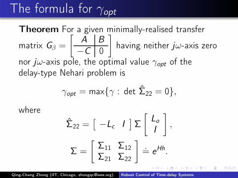
The formula for γopt
Theorem For a given minimally-realised transfer
matrix Gβ =
[
A B
−C 0
]
having neither jω-axis zero
nor jω-axis pole, the optimal value γopt of thedelay-type Nehari problem is
γopt = max{γ : det Σ22 = 0},
where
Σ22 =[
−Lc I]
Σ
[
LoI
]
,
Σ =
[
Σ11 Σ12
Σ21 Σ22
]
.= eHh.
Qing-Chang Zhong (IIT, Chicago, [email protected]) Robust Control of Time-delay Systems

Parametrisation of K
For a given γ > γopt , all K (s) ∈ H∞ solving the problem can beparametrised as
K = Hr (
[
I 0Z I
]
W−1, Q),
where ‖Q(s)‖H∞ < γ is a free parameter and
Z = −πh{Fu(
[
Gβ I
I 0
]
, γ−2G∼
β )},
W−1 =
A+ γ−2BB∗Lc Σ−∗
22(Σ∗
12+ LoΣ
∗
11)C∗ −Σ−∗
22B
−C I 0γ−2B∗(Σ∗
21− Σ∗
11Lc) 0 I
.
Qing-Chang Zhong (IIT, Chicago, [email protected]) Robust Control of Time-delay Systems

Representation in a block diagram
The controller K consists of an infinite-dimensional block Z , which is afinite-impulse-response (FIR) block (i.e. a modified Smith predictor), afinite-dimensional block W−1 and a free parameter Q.
❤
Gβ Z
e−shI
W −1
❤
Q
K❅❅✛
✲-
u
y
z
w
✛
✲
✛✛
✻
✻
✻
❄
❄
Qing-Chang Zhong (IIT, Chicago, [email protected]) Robust Control of Time-delay Systems

Example: Gβ(s) = − 1s−a
(a > 0)
Σ22
ah
aγ
The surface Σ22 with respect to ah and aγ
0 1 2 3 4 5 6 7 8 9 100
0.1
0.2
0.3
0.4
0.5
0.6
0.7
0.8
0.9
1
ah
aγ
aγopt
The contour Σ22 = 0 on the ah-aγ plane
Since I − LcLo = 1 − 4a2γ2, there is∥
∥
∥ΓGβ
∥
∥
∥= 1
2a. As a result, the optimal value γopt satisfies
0.5 ≤ aγopt ≤ 1.
Qing-Chang Zhong (IIT, Chicago, [email protected]) Robust Control of Time-delay Systems

Outline
Notations and some preliminaries
Standard H∞ control problem
Delay-type Nehari problem
Controller implementation
Qing-Chang Zhong (IIT, Chicago, [email protected]) Robust Control of Time-delay Systems
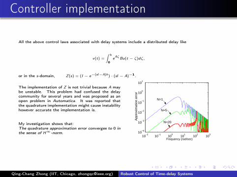
Controller implementation
All the above control laws associated with delay systems include a distributed delay like
v(t) =
ˆ
h
0
eAζ
Bu(t − ζ)dζ,
or in the s-domain, Z(s) = (I − e−(sI−A)h) · (sI − A)−1.
The implementation of Z is not trivial because A maybe unstable. This problem had confused the delaycommunity for several years and was proposed as anopen problem in Automatica. It was reported thatthe quadrature implementation might cause instabilityhowever accurate the implementation is.
My investigation shows that:The quadrature approximation error converges to 0 inthe sense of H∞-norm.
10−2
10−1
100
101
102
103
10−4
10−3
10−2
10−1
100
101
Frequency (rad/sec)
N=1
N=5
N=20
App
roxi
mat
ion
erro
r
Qing-Chang Zhong (IIT, Chicago, [email protected]) Robust Control of Time-delay Systems

Numerical integration
v(t) =
ˆ h
0
eAζBu(t − ζ)dζ
It is well known that
v(t) ≈ vw(t) =h
NΣN−1
i=0 e iAhNBu(t − i
h
N),
but what will happen if transferred into the s-domainusing the Laplace transform?
Zw(s) =h
N· ΣN−1
i=0 e−i hN(sI−A)B
Not strictly proper =⇒ No guarantee of stability !
Qing-Chang Zhong (IIT, Chicago, [email protected]) Robust Control of Time-delay Systems

A trivial result
τ t t−h/N
y(τ)
t 0
y(t) p(t)
t
1
0 h/N
∗=
ˆ hN
0
y(t − τ)dτ =
ˆ t
t− hN
y(τ)dτ = y(t) ∗ p(t),
Qing-Chang Zhong (IIT, Chicago, [email protected]) Robust Control of Time-delay Systems

Approximation of Z
v(t) =
ˆ h
0
eAζBu(t − ζ)dζ
=N−1∑
i=0
ˆ (i+1) hN
i hN
eAζBu(t − ζ)dζ
≈
N−1∑
i=0
e iAhNB
ˆ (i+1) hN
i hN
u(t − ζ)dζ
=N−1∑
i=0
e iAhNB
ˆ hN
0
u(t − ih
N− τi)dτi
=N−1∑
i=0
e iAhNBu(t − i
h
N)∗p(t) = vf (t)
Qing-Chang Zhong (IIT, Chicago, [email protected]) Robust Control of Time-delay Systems

Hidden sampling-hold effect
vw(t) =N−1∑
i=0
e iAhNBu(t − i
h
N)×
h
N
vf (t) =
N−1∑
i=0
e iAhNBu(t − i
h
N)∗p(t)
This is equivalent to the sampling-hold effect.
Qing-Chang Zhong (IIT, Chicago, [email protected]) Robust Control of Time-delay Systems

Implementation in the z-domain
hN ΣN−1
i=0 e ihNABz−i SZOH ✛ ✛✛✛ ✛ uv
(a) Zf (s) =1−e
−s hN
s·∑N−1
i=0 e−i hN(sI−A)B
(eAhN − I )A−1 ΣN−1
i=0 e ihNABz−iZOH S✛ ✛✛✛✛ uv
(b) Zf 0(s) =1−e
−hN
s
se
hNA−IhN
A−1 ·∑N−1
i=0 e−i hN(sI−A)B
Qing-Chang Zhong (IIT, Chicago, [email protected]) Robust Control of Time-delay Systems

Implementation in the s-domain
Zf ǫ(s) =1 − e−
hN(s+ǫ)
1 − e−hNǫ
ehNA − I
s/ǫ+ 1A−1·ΣN−1
i=0 e−i hN(sI−A)B .
limN→+∞ ‖Zf ǫ(s)− Z (s)‖∞ = 0, (ǫ ≥ 0).
10−2
10−1
100
101
102
103
10−4
10−3
10−2
10−1
100
101
Frequency (rad/sec)
N=1
N=5
N=20
App
roxi
mat
ion
erro
r
Qing-Chang Zhong (IIT, Chicago, [email protected]) Robust Control of Time-delay Systems

Rational implementation
The δ-operator is defined as δ = (q − 1)/τ, where q
is the shift operator and τ is the sampling period.We have
δ =eτs − 1
τ
because q → eτs when τ → 0. Define Φ = 1τI and
∆ = (eτ(sI−A) − I )Φ,
then
sI − A = limτ→0
∆, e−(sI−A)τ = (Φ−1∆+ I )−1
Qing-Chang Zhong (IIT, Chicago, [email protected]) Robust Control of Time-delay Systems

Z (s) = (I − e−(sI−A)h) · (sI − A)−1
= (I − e−(sI−A)τN)(sI − A)−1B
= (I − (Φ−1∆+ I )−N)(sI − A)−1B .
Since ∆ ≈ sI − A, Z can be approximated as
Zr(s) = (I − (Φ−1(sI − A) + I )−N)(sI − A)−1B
= (I − (Φ−1(sI − A) + I )−1) ·
ΣN−1k=0 (Φ
−1(sI − A) + I )−k(sI − A)−1B
= Φ−1ΣNk=1(Φ
−1(sI − A) + I )−kB
= ΣNk=1Π
kΦ−1B ,
where Π = (sI − A+Φ)−1Φ.
Qing-Chang Zhong (IIT, Chicago, [email protected]) Robust Control of Time-delay Systems

1x2xΠ
Nx 1−Nx
B1−Φbu
u
rv
…
ΦΦ+−=Π −1)( AsI
Π Π
…
Π = (sI − A+ Φ)−1Φ
In order to guaranteezero static error,
Φ = (´ h
N
0 e−Aζdζ)−1.
Qing-Chang Zhong (IIT, Chicago, [email protected]) Robust Control of Time-delay Systems

Fast-converging rational implementation
Define
Φ = (
ˆ hN
0
e−Aζdζ)−1(e−A hN + I )
Γ = (eτ(sI−A) − I )(eτ(sI−A) + I )−1Φ, τ = h/N
Then,sI − A = lim
τ→0Γ,
sI − A|s=0 = Γ|s=0 = −A,
Γ|sI−A=0 = 0.
Qing-Chang Zhong (IIT, Chicago, [email protected]) Robust Control of Time-delay Systems

1x2xΠ
Nx 1−NxB u
rv
…
)()( 1 Φ+−Φ+−=Π − sIAAsI
1)(2 −Φ+−=Ξ AsI
Π Ξ
…
Π = (Φ− sI + A)(sI − A+ Φ)−1,
Ξ = 2(sI − A+ Φ)−1
10−2
10−1
100
101
102
1010
−4
10−3
10−2
10−1
100
101
Impl
emen
tatio
n er
ror
Frequency (rad/sec)
δ−operator
discrete delay
bilinear trans.
Qing-Chang Zhong (IIT, Chicago, [email protected]) Robust Control of Time-delay Systems

Summary
Standard H∞ control problem
Delay-type Nehari problem
Controller implementation
Qing-Chang Zhong (IIT, Chicago, [email protected]) Robust Control of Time-delay Systems

Qing-Chang Zhong (IIT, Chicago, [email protected]) Robust Control of Time-delay Systems