risk management in project finance - de-brouwer.com · risk management in project finance by dr....

RISK MANAGEMENT IN PROJECTFINANCE

by

DR. PHILIPPE J.S. DE BROUWERLECTURER AT VLERICK BUSINESS SCHOOL AND UNIVERSITY OF WARSAW; AND HEAD ANALYTICS

DEVELOPMENT AT ROYAL BANK OF SCOTLAND GROUP)

WWW.DE-BROUWER.COM * [email protected]

OCTOBER 3, 2015

UNIVERSITY OF WARSAWCLUSTER:

“FINANCE”

SECTION: FINANCE

http://www.de-brouwer.com

mailto:[email protected]

Contents

Nomenclature 101

List of Figures 107

List of Tables 109

I Risk Management 111

1 Introduction 113

2 Integrated Risk Management and the Risk Cycle 117

3 Risk Identification 1213.1 Specific Types of Risk . . . . . . . . . . . . . . . . . . . . . . . . 1233.2 Generic Risk Factors . . . . . . . . . . . . . . . . . . . . . . . . 123

4 Risk Assessment and the Risk Matrix 133

5 Risk Quantification 1375.1 In Search of a Risk Measure . . . . . . . . . . . . . . . . . . . . 138

5.1.1 Variance as a Risk Measure . . . . . . . . . . . . . . . . 1395.1.2 Value at Risk (VaR) . . . . . . . . . . . . . . . . . . . . . 1475.1.3 Expected Shortfall (ES) . . . . . . . . . . . . . . . . . . . 156

5.2 Risk Modeling . . . . . . . . . . . . . . . . . . . . . . . . . . . . 1635.2.1 Stress Testing . . . . . . . . . . . . . . . . . . . . . . . . 164

CONTENTS

5.2.2 Monte Carlo Simulations . . . . . . . . . . . . . . . . . 1655.2.3 Beyond the Monte Carlo Simulation . . . . . . . . . . . 167

6 Conclusion 173

II Addenda 177

A Coherent Risk Measures 179A.1 Introduction . . . . . . . . . . . . . . . . . . . . . . . . . . . . . 179A.2 Definitions . . . . . . . . . . . . . . . . . . . . . . . . . . . . . . 180

A.2.1 Coherent Risk Measures . . . . . . . . . . . . . . . . . . 180A.2.2 Variance (VAR) . . . . . . . . . . . . . . . . . . . . . . . 182A.2.3 Value at Risk (VaR) . . . . . . . . . . . . . . . . . . . . . 182A.2.4 Expected Shortfall (ES) . . . . . . . . . . . . . . . . . . . 183A.2.5 Spectral Risk Measures . . . . . . . . . . . . . . . . . . . 186

A.3 The Consequences of Thinking Incoherently . . . . . . . . . . 187A.4 Portfolio Optimization and Risk Minimization . . . . . . . . . 190

A.4.1 Value at Risk (VaR) . . . . . . . . . . . . . . . . . . . . . 190A.4.2 Variance (VAR) . . . . . . . . . . . . . . . . . . . . . . . 192

A.5 Regulatory Use of Risk Measures . . . . . . . . . . . . . . . . . 193A.5.1 Using VaR as a Risk Limit . . . . . . . . . . . . . . . . . 193A.5.2 What about Stress Tests? . . . . . . . . . . . . . . . . . . 193A.5.3 How could banks be safer? . . . . . . . . . . . . . . . . 194

A.6 Conclusions . . . . . . . . . . . . . . . . . . . . . . . . . . . . . 194

B Levels of Measurement 197B.1 Nominal Scale . . . . . . . . . . . . . . . . . . . . . . . . . . . . 197B.2 Ordinal Scale . . . . . . . . . . . . . . . . . . . . . . . . . . . . . 197B.3 Interval Scale . . . . . . . . . . . . . . . . . . . . . . . . . . . . 198B.4 Ratio Scale . . . . . . . . . . . . . . . . . . . . . . . . . . . . . . 199

Bibliography 201

Author Index 207

Index 209

100

Nomenclature

α a level of probability, α ∈ [0, 1] (to characterize the tail risk α will be“small”—for example for a continuous distribution one can say with aconfidence level of (1−α) that the stochastic variable in an experimentwill be higher than the α-quantile), page 186

ı a column vector where each element equals one, page 142

Σ the varcov matrix, page 142

w the vector of weights of rank M , so that∑Mi=1 wi = 1, page 140

x′ the transpose of the vector or matrix x, page 140

δ(.) the Dirac Delta function: δ(x − a) =

{0 if a 6= x

+∞ if x = a, but so that∫ +∞

−∞ δ(x− a) dx = 1, page 186

R the set or real numbers, page 180

V the set of real-valued stochastic variables, page 180

N The set of natural numbers = {0, 1, 2, . . . , n, . . . }, page 157

R the set of real numbers, page 196

L a loss variable expressed in monetary terms, page 148

P a profit variable expressed in monetary terms, page 148

NOMENCLATURE

µ the average or expected value of a stochastic variable X , page 182

µ the average or expected value of a stochastic variable x, page 140

µp the expected return of portfolio p (consisting of M loans), page 142

φ(p) the risk spectrum (aka risk aversion function), page 186

ρ a risk measure, page 181

ρ the correlation coefficient), page 142

ρij the correlation between asset i and asset j, page 142

σi the standard deviation of the return of asset i, page 142

σp the (expected) variance of portfolio p, page 142

σij the covariance between asset i and asset j, page 142

c a real number: c ∈ R, page 143

ess.infacerbi2002expected essential infimum, page 161

F (x) the cumulative distribution function, page 147

F−1(α) the inverse of the cumulative distribution function, by definition leftcontinous, page 147

fR(t) the density function of a continuous distribution of a stochastic variableR, page 140

fX(t) the probability density function of a continuous distribution of astochastic variable X , page 182

FX(x) the cumulative distribution function of the stochastic variable X ,page 186

fest(x) the estimator for the probability density function, f(x), page 168

fest(x;h) the estimator for the probability density function for a kernel densityestimation with bandwidth h, page 168

h the bandwidth or smoothing parameter in a kernel density estimation,page 168

i counter, page 140

102

NOMENCLATURE

i counter, page 182

inf infimum, page 161

int(.) used as a function, int(.) extracts the integer part of its argument,page 157

Kh the kernel (of a kernel density estimation) with bandwidth h, page 168

Mφ(X) a spectral risk measure, page 186

p a probability (similar to α), page 186

qα(X) the α-quantile of the stochastic variable X , page 182

QX(p) the quantile function of the stochastic variable X , page 184

QX(α) the quantile function of the stochastic variable X , page 147

q(α) the α-quantile, page 147

R return, page 139

Rp the return of portfolio p (consisting of M loans), page 142

S semi-variance, page 144

sup supremum, page 161

X a real valued stochastic variable, representing a profit variable,page 182

x−

{x if x ≤ 0

0 if x > 0, page 144

ABS Asset Backed Securities, page 124

AS Average Shortfall, page 157

AVaR Average VaR, page 157

CDS Credit Default Swap, page 135

CF Cash Flow, page 135

CF Cash Flow, page 164

103

NOMENCLATURE

CFR Cash Flow Risk, page 129

EAD Exposure At Default, page 137

ECA Export Credit Agency, page 122

EL Expected Loss, page 137

ELTIF European Long-Term Investment Fund, page 175

ES Expected Shortfall, page 184

ETL Expected Tail Risk, page 157

IRR Internal Rate of Return, page 164

IRS Interest Rate Swap, page 128

KDE Kernel Density Estimation, page 167

LBO Leveraged Buy-Out, page 124

LEP Large Electron Proton Colider, page 126

LGD Loss Given Default, page 137

LRL Limited Recourse Lending, page 114

MCDA Multi Criteria Decision Analysis, page 119

MISE mean integrated squared error, page 169

NPV Net Present Value, page 164

p2p “peer to peer”, page 194

P&L Profit and Loss, page 165

PD Probability of Default, page 137

pdf probability density function, page 138

SLA Service Level Agreement, page 119

SPV Special Purpose Vehicle, page 114

TCE Tail Conditional Expectation, page 157

104

NOMENCLATURE

VAR variance, page 182

VaR Value at Risk, page 148

VaR Value at Risk, page 182

VB Visual Basic, page 165

WPM Weighted Product Method, page 119

105

List of Figures

1.1 Project Finance . . . . . . . . . . . . . . . . . . . . . . . . . . . . 114

2.1 The Risk Management Cycle . . . . . . . . . . . . . . . . . . . . 118

5.1 Mean variance optimization for 3 loans . . . . . . . . . . . . . 1415.2 VaR Portfolio Optimization . . . . . . . . . . . . . . . . . . . . 1505.3 VaR and cdf for default risk . . . . . . . . . . . . . . . . . . . . 1515.4 cdfs for default risk . . . . . . . . . . . . . . . . . . . . . . . . . 1525.5 continuity as a function of α for ES and VaR . . . . . . . . . . . 1535.6 ES and VaR for default risk . . . . . . . . . . . . . . . . . . . . 1545.7 the efficient frontier for ES and VaR for default risk . . . . . . 1555.8 Expected Shortfall . . . . . . . . . . . . . . . . . . . . . . . . . . 1605.9 Risk measures compared . . . . . . . . . . . . . . . . . . . . . . 1625.10 Epachenikov and Gaussian kernel . . . . . . . . . . . . . . . . 1705.11 histogram of annual returns . . . . . . . . . . . . . . . . . . . . 171

A.1 VaR and ES in function of α . . . . . . . . . . . . . . . . . . . . 185A.2 ES and VaR for default risk . . . . . . . . . . . . . . . . . . . . 189A.3 the risk surface for VaR and ES . . . . . . . . . . . . . . . . . . 191

List of Tables

1.1 Examples of project failures . . . . . . . . . . . . . . . . . . . . 115

3.1 Similaries and differences . . . . . . . . . . . . . . . . . . . . . 124

4.1 risk matrix template . . . . . . . . . . . . . . . . . . . . . . . . 135

B.1 Nominal Scale of Measurement . . . . . . . . . . . . . . . . . . 198B.2 Ordinal Scale of Measurement . . . . . . . . . . . . . . . . . . . 198B.3 Interval Scale of Measurement . . . . . . . . . . . . . . . . . . . 199B.4 Ratio Scale of Measurement . . . . . . . . . . . . . . . . . . . . 200

Part I

Risk Management

Chapter1Introduction

Large infrastructure works such as building highways, airports, power sta-tions, harbours are most important tools to improve directly comfort andwell-being or indirectly by fueling economic development. The World Bank,for example, estimates that a ten percent increase in infrastructure projectsleads to a one percent increase in GDP —(Calderon, et al. 2011); hereby con-firming (Evans & Karras 1994)’s findings.

In Asia alone the global pipeline is estimated at $ 9 trillion (Beckers,et al. 2013), this is more than half the GDP of the USA. The United King-dom currently plans to engage in roughly 500 projects that would total £ 200billion in the next 5 year and will cost £ 500 billion by 2020 – see (gov.uk 2015,Coopers 2015).

Project Finance or Limited Recourse Finance1 is typically defined as:

Definition 1.0.1 (Limited Recourse Finance). A form of financing –typically a large and capital intensive infrastructure– project where thelender gains confidence that the borrower is able to service the loan notby its creditworthiness but via a claim on future cash flows.

1We will use the terms “Project Finance” or “Limited Recourse Finance” interchangeably.

CHAPTER 1. INTRODUCTION

We will use the words Limited Recourse Financing, Limited RecourseLending and Project Finance as synonyms and use the shorthand notationLRL.

The reason why the lender can not grant the loan based on the balancesheet of the borrower is that the borrower is typically as Special PurposeVehicle (henceforth SPV), that is only created for the purpose of the projectand hence has no credit history and little asset other than the project.

Sponsorsequity

))

Lenders

loans��

Government

land leasevvbudget allocation

��

SPV

contractsuu

agreements

((Engineering Companies Operating Company

Figure 1.1: A simplified schedule of a typical project finance setup. In reality there are moreflows and agreements. For example the sponsors will need a Shareholders Agreement, thegovernment might give credit support to the SPV and/or the Operating Company. Othervariations are possible, for example the Operating Company might be a government institution,if the government is not the off-taker then no budget allocation is needed, etc. Each project isunique.

A few definitions will make the concepts introduced in Figure 1.1 clear:

• Government: the government or other authority involved is the onethat would like the benefits of the project to be available but lacks thefinancial strength and technological know-how to run the project itself.Typically the government(s) will initiate the projects and even run a ten-der between competing groups of companies. The Government selectsthe winning group by allocating to them the permission to use the land.

• Sponsor(s): one or more companies that have an equity stake in theSPV. This company is hence owner of the SPV and due to their technicalknowledge should be able to contribute to the management of the SPV.Typically a Sponsor is a company that has experience in executing similarprojects and/or has an interest in the project being executed.

• Engineering Company: the Engineering company is the company that

114

will execute the building of the project. It might do so directly and/orsubcontract.

• Lenders: the Lenders are the financiers of the project, they are the partythat will “invest” the largest amount by granting loans, that typicallyare up to ten times larger than the equity investment of the Sponsors. Inorder to diversify these huge risks, lenders will organize themselves insyndicates and may include government agencies.

• Operating Company: is a general word used in Figure 1.1 on the pre-ceding page that can be Tolling Company, the Operating Company andeven the Off-Taker would fit in the same place.

The benefits are important, the amounts involved are huge and so is thecomplexity in all possible aspects.

Project (Country) plannedcost (e bil-lion))

actual cost(e billion)

Reason

Betuweroute(Netherlands)

e 2.3 e 4.7 1.5 year delay, finally in use in 2007,partly not finalized (planned 2020)

Eurotunnel (France/ UK)

e 7.5 e 15.0 6 month delay, 18 months of unreli-able service after opening, marketshare gain overestimated by 200%

Rail Frankfurt-Koln (Germany)

e 4.5 e 6.0 unforeseen capped governmentspending, legal issues, 1 year delay

Kuala Lumpur Air-port (Malaysia)

e 2.0 e 3.5 losing market share to Signapore(runs at 60% of capacity), issueswith connection to downtown area,complaints about health and safety

Table 1.1: Examples of infrastructure projects that failed to deliver in time. (source Reuters,McKinsey, Wikipedia, annual reports)

Table 1.1 lists a few examples of infrastructure projects that did cost moremore than planned. These examples are by no means exceptions. Most issuesseem to be with delays related to engineering and production, inadequate fore-casting of markets share, funding issues, competitive landscape, etc. Modern

115

CHAPTER 1. INTRODUCTION

infrastructure projects are large and complex, but it seems to us that most ofthe loss of value for the society can be avoided by adequate risk management.

Larger projects typically overrun budgets or fail on a set of issues that canbe summarized as:

• engineering problems delay the delivery of the project;

• the benefits of the project are overstated or do not fit in a larger strategy(for example a railroad should fit in a national mobility plan);

• financial resources do not become available as planned;

• design issues.

The good news is that therefore –it seems to us– a large part of these risks canbe mitigated by a a modern, comprehensive and end-to-end risk managementprocess that is embedded in a true risk culture. The rest of this section will tryto make that point by presenting how the risk management should work andencompass all stages of the project.

116

Chapter2Integrated Risk Management andthe Risk Cycle

Limited Recourse Financing or Project Finance exists mainly because (a) largeinfrastructure projects are necessary and useful for economic development and(b) that in order to execute these projects risks have to be shared or transferredto parties that can bear the risk better. This aspect together with the sheersize of the projects –both in time and money-terms– will make clear that riskmanagement is one of the most important aspects of a successful project.

Since the project takes a lot of time and not in all phases the risks are thesame it is important to maintain a continous cycle of risk identification, riskmitigation and risk management. Figure 2.1 on the next page illustrates thiscycle of risk management. Every party involved will have to do its own riskmanagement and use his own point of view while going throught this cycle.

The fact that involved parties can push risk from one company to anothermeans that the risks are different for each party involved and that what is “amitigation” for one party can be “a new risk” for another party. For examplethe SPV is faced with the risk of late ending of the construction phase (thiswill not only delay the income but it might be possible that in the meanwhilethe SPV is already responsible for paying back some loans). So the SPV willmitigate that risk by adding a late delivery clause to the contracts of theengineering companies. So, now the SPV is covered while the engineeringcompanies took that risk on board. This risk allocation seems reasonablebecause it is the engineering company that will execute the work and should

CHAPTER 2. INTEGRATED RISK MANAGEMENT AND THE RISK CYCLE

risk identificationif possible +3 risk mitigation

residual risk��

risk management

review

KS

risk reclassificationks

Figure 2.1: Risk Management is an ongoing concern of utmost importance. Phase after phase,cycle after cycle and for each party one will have to go through this cycle in order to mitigateand minimize risks. Bad risk mangement is bound to lead to disaster.

be best placed to assess the time needed to do the work and it is the only partythat can act by for example adding more workers in order to assure a timelycompletion of the job.

Please note that in this example the late delivery risk is not completelycovered for the SPV, in fact it became a risk related to the creditworthiness ofthe engineering company.

So, each party will have a different view on what is risk and how to manageit. What each company involved should do is create insight in the relevantrisks, mitigate if possible and continuously follow up the main risks and makesure that they remain minimized. For example it is not sufficient to identifythe risk that the construction phase may end late, it is only by following upevery day and speeding up the process that the damage can be minimized.

Therefore each party should on an ongoing base cycle through the follow-ing aspects:

1. Identify Risks. Of course the main risks can be indicated by followingthe checklists provided in Chapter 3 on page 121, but it is necessary toreview on a regular base. Some risks might have been dormant andmight not have been identified at all or emerge as the fallout from theemanation of another unexpected risk. This new risk should be addedto the list, mitigations have to be put in place and the risk has to bemanaged to keep the fallout under control.

2. Assess the Impact and Probability. It is not sufficient to look only atprobability or only at impact when assessing a risk, it is absolutelynecessary to monitor both dimensions. Also probability and impact willvary during the lifetime of a project (for example when a project is built,the risk of delayed construction falls to zero). As it is often impossibleto quantify accurately these impact and probability parameters, one

118

typically resorts to an ordinal scale1, such as Very Low, Low, Medium,High and Very High or simply a number between 1 and 5.2

3. Mitigate Risks. Where possible, risks will be mitigated. For example ifthere is a risk that the construction phase of the project will be delayed,then the SPV can put a “delayed delivery clause” in the contract andwill make sure that there is a liquidate damages clause. The engineeringcompany on its turn mitigates this risk by assuring that the deadlinesare realistic, that –where subcontractors are used– their contracts reflectthis clause, and –for own workers– it will make sure that that workforceis managed well and that a good risk management is in place.

4. Calculate residual impact and probability and re-classify. Obviously,risk will change as it is managed well. Assume that we identified thebreakdown of a concrete pump as a critical risk and now we have SLA(Service Level Agreement) in place with a provider that assures us tohave a new pump on our site within 48 hours. In that case the riskrelated to the concrete pump must be re-assessed and certainly will notbe critical any more. This example show us that the risk manager whodoes his job well will permanently shift focus: now that the concretepump is under control he/she will go after the next important risk andtry to mitigate it too.

5. Prioritize Risks. Based on the above two dimensions one is able to makea classification of all risks in a one-dimensional way based on a MCDA(Multi Criteria Decision Analysis), typically something related to WPM(Weighted Product Method) is most appropriate. This prioritization canbe presented as a “risk matrix” (see Chapter 4 on page 133).

Now that all the aspects are in place, it is essential to make sure that riskmanagement becomes a cornerstone of the engagement, an ongoing concernand the focus of all. This is done by having a risk manager in place that is–preferably– at the level of the executive committee of the relevant organizationand that a true risk culture is in place. It is everyones responsibility to spotrisks, help to mitigate them and prevent them from realizing. When risks dohave to be taken, it is worth to consider if the payoff of a given risk fits in ourrisk appetite (in other words if it the return is worth the risk).

1See Appendix B on page 197.2In most cases a scale with 5 levels will work pretty well: it is not too rough (such as High,

Medium and Low) and still is a lot simpler than a “real number between 0 and 1” approach.However it cannot be stressed enough that such scale is only an ordinal scale and not an intervalscale and this has important impact: see Appendix B on page 197 for further information.

119

CHAPTER 2. INTEGRATED RISK MANAGEMENT AND THE RISK CYCLE

In the next chapters we will clarify these important steps in risk manage-ment.

120

Chapter3Risk Identification

As mentioned, Project Finance can be seen as a way to reallocate risks to theparty best fit to take a certain risk on board. Each project is a delicate exercisein refining and re-organizing risk allocation up to such level that the project isboth realistic and profitable for each participant. It will be clear to the readerthat since Limited Resource Lending exactly exists because involved risks aretoo high that risk management is an essential part for each player in the setupand execution of any project.

Each participant will have his own reasons to participate and his own pointof view on the risk. To understand better the deepness of this idea, we explorethis from the different participant’s point viewpoint.

• the Sponsor(s): even large construction companies do not have theresources to finance biggest projects and if they would bring up thefinance via lending for example, one failure would bring them down.Banks are by their nature better able to diversify risks (that is actually thereason why banks grew so big since the rise of the Banque de Rothschildin the era of the Napoleonic wars). Also one will notice that the Sponsorsspecialize in execution of similar projects and do not specialize in largefinancial risk taking. That is another business model.

• the Government: large infrastructure projects are important for the econ-omy, however they typically span multiple political cycles. Thereforeit is less appealing for politicians to do the hard work and get a projectstarted only to see financial resources consumed and basically preparethe field for the opponent to harvest the economic advantage of the

CHAPTER 3. RISK IDENTIFICATION

project and the political public relations that go with the opening of theproject. Therefore it is more appealing to become the “initiator” and usethe financial resources for spendings that will yield shorter term payoff.Gornments can hence use LRL as an alternative to raising money on thebond market (examples of this form of funding are for example the “warbonds” in many countries — early examples are the city states in Italy inthe Middle Ages). The reason to do so typically boils down to one of thetwho following problems: or the country is too small and weak to takeon the risk or the country is large and strong but has too man projects onthe agenda. A good solution is then to use the leverage in the bankingsystem.1

• the Lenders: the largest financial risk ends up with the lender. Of coursethat lender can try to mitigate risks as good as possible –as we willdiscuss later– but even that will typically be insufficient and thereforewill seek to diversify and prefer to lend £ 50 to two projects in stead of£ 100 to one and take in each project another lender as partner and henceforming as syndicate. However –also after the Global Meltdown of 2008–this form of of collaboration became more difficult and more and morethere is the tendency to resort to consortium2 collaboration betweenbanks. But the pressure on investment banks is so intense that they can-not longer play their natural role in our economy to the extend that oureconomy needs. So, more and more one resorts in putting the taxpayer’smoney directly at risk. This is done by copying the “off-balancing mecha-nism” –that leveraged banks to an unreasonable extend and was directlyresponsible for the Global Meltdown– to governments. The credit expo-sure is not kept on the balance of the government, but rather hidden inoff-balance SPV’s called “Export Credit Agencies” (henceforth ECAs).3

So, all parties involved in the project will have their own specific point ofview on the project and along with that their specific risks and needs in risk

1Although, as we already noted the recent crackdown on banking and investment banking inparticular (see for example the Basel III requirements) puts automatically and directly the riskand burden with the governments in stead of having banks as a first safety layer.

2The concepts of “loan syndication” and “consortium” are very close and both sport oneborrower and multiple lenders that share the risk. Typically the difference is understood as suchthat a syndication is geared towards international collaboration (involving multiple currencies)and has one clear “managing bank” that assures a technical lead –not necessarily the largestlender.

3This could be seen as how a mechanism that is installed to solve one crisis typically seeds thegerms for the next crisis. For example, the off-balancing mechanism (that produced the GlobalMeltdown) was introduced by the Clinton administration to remedy the banking problems of theeighties.

122

3.1. SPECIFIC TYPES OF RISK

management. As the Lender is the party that risk the most money and hasleast control over what is happening on the field, it is an interesting point ofview for risk management. Unless otherwise stated we will use in the nextsections the point of view of the Lender.

3.1 Specific Types of Risk

We defined Limited Recourse Lending (LRL) in Definition 1.0.1 on page 113.From this definition follows automatically that some very specific types of riskmust exist.

This implies immediately that Project Finance will have some very specificforms of risk that are typically not or rarely present in other forms of lending.We consider the following aspects as quite unique for Project Finance:

• no credit-worthy borrower but reliance on future cash flows: thismeans that the business risk is not borne by the sponsor, but rather bythe lender

• size: projects are constructed as a LRL project, because nor the sponsor(s)nor the government are able or willing to bear the risk alone and hencethe risk is transferred to investment banks4

• typically for large infrastructure projects: although sometimes univer-sities and even prisons are build in the form of project finance, typicallyonly durable infrastructure projects are deemed important enough.

3.2 Generic Risk Factors

Besides having its particular risk factors, that seldom appear in other projectsand ventures, Project Finance also shares a large base of risk factors that arecommon with other types of financing. Of course, due to the size of the projectthe risks involved are much larger in a LRL project and some of the risks willbe specific to different LRL constructions.

For example:

4Since the Global Meltdown (2008) banks are under much pressure to de-leverage, keep moreliquidity and hence are less able to finance large and risky projects. This is of course what theregulator wants: banks had to become safer, but of course by doing so the risk is now more andmore borne by Export Credit Agencies . . . so, directly by the taxpayer.

123


FinancingForm

Similarities Differences

corporatelending • the structure of the loan

is a “term loan”

• the risk of the lender isrelated to the ability ofthe borrower to generatecash flows

• the comfort that the loan willbe repaid is based on futurecash flows of the project andnot by the creditworthinessof the borrower

• the asset that could serve ascollateral does not exist yet inLRL

ABS (AssetBacked Se-curities)

• the borrower is an SPV

• the originator (“Spon-sor” in LRL) obtains “off-balance sheet financing

• the SPV issues bonds in steadof lending from bank(s)

• in ABS one has a large poolof assets (eg. loans); in LRLthere is one large asset

VentureCapital,BusinessAngels

• the borrower has (almost)no creditworthiness

• the lender relies mainlyon future cash flows

• in LRL the SPV is highlyleveraged

• the Venture Capitalist pro-vides typically an equitystake and not a loan

LBO(LeveragedBuy-Out)

• the borrower has limitedcreditworthiness

• both are highly leveragedtransactions

• the lender has typically re-course on the borrowers,

• in LBO the lender can hopethat the borrower gains cred-itworthiness

Table 3.1: Similarities and differences with other forms of financing.

124

3.2. GENERIC RISK FACTORS

• Feasibility Risk or Technology Risk: of course the first thing to assessis if the project is possible. For example is there oil where we want todrill? And if the project itself makes sense it is important to address thequestion if the project is viable. For example will the pipeline be able tocarry the flow that is needed to get the required returns? While this isto a large extend an engineering problem, that only the best specialistscan answer it is also a relevant risk to the Lender. If the lender wouldlend to an unrealistic project, then the project will fail, the SPV will gobankrupt and the loans will not be paid back. So, the Lender will haveto engage specialist advisors.

• Natural Disasters / Force Majeure: Some events –such as a nearby su-pernova blast in “nearby stars”, super-volcano’s, comet impacts, etc.–are not possible to predict yet, have the potential to destroy the civiliza-tion as we know it and even all life on earth. Our practical knowledgeon such events is limited, but from the fossil record we can tell thatthe probability of such event to occur is extremely low.5 Therefore it isboth impossible and unnecessary6 to try to mitigate such risks withinthe framework of an infrastructure project.7 However, there are much–smaller– events that can and should be taken into account. Naturaldisasters such as earthquakes, floods, etc. are exactly both probable andsizable enough so that they have to be taken into account of the design

5An extinction event (also known as a mass extinction or biotic crisis) is a widespread andrapid decrease in the amount of life on Earth. Such an event is identified by a sharp change inthe diversity and abundance of macroscopic life. The fossil record of the last 550 million yearsshows every fifty to hundred million years an extinction event. In many cases they mark thetransition to another era where new species dominate sea, land and air. Probably the best knownextinction event is the CretaceousPaleogene extinction event (66 Ma ago) when the Chicxulubimpactor ended the reign of the dinosaurs. However, the most eye-catching one is in our opinionthe Holocene Extinction Event that started 10’000 years ago and is still ongoing. The reasons ofthe Holocene Extinction Event can be summarized in one word: humans.

6It is impossible to take such risks into account because we do not know exactly when the nextsupernova will blast (or more precisely: “has blasted” – if for example WR104 in Sagittarius hasblasted 7999 years ago, –and assuming it is exactly 8’000 light-years from us– then its X-rays willwipe out most macro-biotic life next year when its X-rays destroy ozone layer and most complexmolecules such as DNA.) Also it is unnecessary to take such risks into account: if indeed WR104exploded 7999 years ago and next year all complex life will be wiped out on earth then, indeed, itwould not matter that our railroad will not be finished.

7Indeed Extinction Events have happened in the past and will happen in the future, we cannottake them into account in risk management of our project (such as an airport, highway or a bridge),but the mathematical certainty that life will be wiped out on this planet will make an excellentLRL project for the future: build the technology and machines to spread humans or their intellectbeyond this planet. This however requires a planetary effort of a planetary society with a unifiedhumanity. Our guess is that this is at least a few generations ahead.

125


of the project (eg. the bridge will have to be strong enough and mustnot move with the resonance frequency of the wind-force such as theTacoma Narrows Bridge in 19408) and can and should be insured (bothbefore, during and after the construction phase of the project).

• Cost Overrun: Every project can end up more expensive than initiallyplanned: from a refitting of one’s bathroom to the building of a nuclearpower station. This can have many causes: materials used, price inflationof the materials, (un-hedged) currency exchange risk, strikes, etc. Butprobably the most important factors for large projects are the TechnologyRisk and the Completion Delay.

• Technology Risk: Typically in LRL the technical details of the designproject are not known in advance9 The more experienced the Sponsoris, the less risk there should be, but many complex projects need still alot of the planning to be done when the deal is struck.10 Also in manycases the technology might not exist or is being used for the first time(eg. building an Airport on the sea –Hong Kong– or building a 27kmlong Electron-Proton Colider under Geneva.)

• Completion Delay: As in all projects, some tasks “lie on the critical path”and will delay project delivery if not closed in time. Since large projectshave so much dependencies, it is unreasonable to expect that nothing willgo wrong. In many cases the large losses or reduced profitability incuredis due to a delayed completion of the project (eg. the Betuweroute –asmentioned in Table 1.1 on page 115– is a project where Completion Delaycaused the costs to double and the benefits to be much later availablefor the economy). This risk will typically end up with the Engineeringcompany that contracts to build a certain part. The SPV for the projectwill typically foresee penalties for late delivery.

8The failure of the Tacoma Narrows Bridge in 1940 is a classical textbook example of manyphysics and engineering handbooks. See for example Ohanian (1994), Wikipedia (2015) or thepaper Billah & Scanlan (1991)

9One counts on the winning consortium of Sponsors to fill in these details. This is very differentfrom the projects where authorities are the direct and sole owners of the project, in that casethey typically have a very detailed order book ready and the bidding is typically focused aroundpricing.

10There are many reasons for the limited availability of project details at the start of the projects.First of all it would be very costly and take too much time to plan all details in advance, on topof that certain aspects will only be discovered as the building starts and then plans have to beadapted anyhow. Also one can argue that project details don’t have to be submitted to win thetender.

126


• Credit Risk: This form of risk is the risk that a lender bears when lendingmoney to a borrower. The risk is obviously related to the (in)capacity ofthe borrower to service the loan. As in Project Finance the borrower is anSPV –with little equity compared to loans on its balance sheet– this riskbecomes particularly important for the lender(s). As a mitigation for thelack of creditworthiness of the SPV, the lenders will seek claims on theconstruction and/or exploitation rights of the project. As the reader willunderstand this makes the lenders most exposed around the deliveryphase, when all the credit is drawn but the security (the project) is notyet producing any cash flows.

• Cash-Flow risk: The risk is here that the project is not able to deliver thecash flows that were planned. This can be due to many reasons, but themost obvious are related to

– the risk that the sales of the project’s product is lower,– that the input materials are not available or more expensive (Feed-

stock Risk),– that input materials are more expensive because of the exchange

rate (Currency and Exchange Risk),– that interest rates rise to that the borrower cannot service the loans

appropriately (Interest Rate risk).

• Sales Risk or Off-Taker-Risk: This is the risk that once the product isready that there is less demand for the product. For example electricityfrom windmills might substitute energy from a nuclear power plant.These changes can be a result from market dynamics related to the project(eg. transport by road and water took already the market for the newrailroad because it took so long to build it), or reflect political changes(eg. a negative attitude towards air travel, nuclear power, etc.). In casethat the off-taker is a large company and not the entire population theSPV will typically seek contracts of minimal take-off (eg. an oil refinery,pre-selling oil at a given price to the Tolling Company).

• Feedstock Risk: This is the risk that the fuel needed to run the installa-tion that is being build becomes scarce and/or expensive. This can berelated to political risk (eg. oil will become both scarce and expensivewhen war rages in the Middle East), pure supply limitations (eg. wardestroyed part of the production capacity). If prices of the Fuel will goup, then also this will squeeze the cash-flows of the project that in theirturn deteriorate the credit quality.

127


• Financial Market-Risk

– Currency and Exchange Risk: This is the risk related to adverseprice changes for fuel, materials, labour, etc. because of fluctuationsof the exchange rate of relevant currencies. This risk can be hedgedvia derivatives on the relevant exchange rate. Different options areopen for the investors, such as forwards (with fixed conditions) andoptions (which don’t have to be exercised when they end out to themoney). For example when one runs a project in GBP and needsto buy some materials for $ 10mln. then it is possible to get intoan agreement and buy the currency today at a price that is fixedtoday (the forward price), with delivery and payment when thecurrency is needed. Alternatively, one can speculate that the dollarmight decrease in value and not lock in the exchange rate today: inthat case one buys a call option on Dollars with nominal $ 10mln.That option can be bought now (payment up-front) or paid “as aninstallment”, called a SWAP agreement.

– Interest Rate Risk: When the interest rate risk of a loan is not fixed,but depends on a market rate, then interest rate risk occurs forthe borrower. When interest rates rise faster than his earnings, hemight struggle to repay the loan. Therefore bankers will typicallynot propose a term loan at a fixed interest rate but rather a loan thatis to be repaid at a floating interest rate and an IRS11. The reasonswhy banks would rather not package these deals were that thiswas beneficial for their balance sheet as the latter would be “off-balance”. Obviously, this created some confusion for the buyers ofsuch contracts.12

• Political Risk: this form of risk is related to the fact that political au-thority is not always very stable and that while a certain governmentprocures the project now, by delivery of the project there might be agovernment that is hostile to the project. Other –related– forms of risksare the “regulatory risk”. For example while the power station is being

11IRS stands for Interest Rate Swap. This is the derivative transaction where party A (the bank)promises to provide the difference between a floating interest rate and a fixed one. Party B (theborrower in our case) hence gets from party A the fixed interest minus the floating, the result isthat party B can repay the loan on a fixed interest rate known in advance.

12The IRS will basically provide positive income for the buyer when interest rates rise (so thatthe effect of this rise is canceled out), but if interest rates increase then the value of the negative.This means that if the borrower wants to pay back his loan he still has to pay a significant amountto break the IRS.

128


built, the authorities might add controls, guidelines and procedures.This might result in –some parts– of the project having to be rebuilt forexample, or simply more costly procedures are needed as a license tostart operation seems suddenly elusive. For example in 2015 the UKgovernment decides to stop subsidizing new onshore windmills, thiswill not impact existing projects too much (maybe they might even get abetter price for their electricity), but it is not unknown that governmentschange the rules of the game while playing.

• Model Risk: finally all the above mentioned risks are put into a statisticalmodel that is supposed to find out if the returns are worth the risks. Suchmodel is never perfect and and the expected deviation of this modelwith the reality is called “model risk”. The model can for example beover-fitted on on too many variables, or a the set of historic data is simplynot representative for the future risk.Of course there is also another type of model involved: the models thatthe engineers use to calculate the amount of material used for example.Also these models are critical, if the engineers get it wrong the structurewill not be strong enough.

As the reader will notice, the different forms of risk can interact, shift fromone form to another and even many of the risk definitions used are overlappingor could be classified in other ways (eg. Financial Market Risk could be acombination of both Exchange Rate Risk and Interest Rate Risk) and mostrisks are can be summarized as “Cash Flow Risk”. For example a technologyrisk might realize itself (eg. while building the subway in Warsaw –in 2013–many problems with water entering tunnels and movements in the sandyground appeared. This technology risk resulted in a Time Overrun Risk, thaton its turn causes that the subway will be opened later, and hence incomingcash flows will be later in the project while earlier on there were higher costsdealing with the problems underground. Almost all risks somehow will beconverted into Cash Flow Risk (henceforth CFR). Getting this CFR correct istherefore crucial, but to get that correct it is essential to understand all othertypes of risk.

Cash Flows can be modeled with a wide range of approaches. A simplespreadsheet such as Libre-Office-Calc or Mircrosoft Excel can get you a longway in order to get a view on the big picture of the project. This “big picture”is always good to have and is not really replaced by more detailed simulations.

However to fully model the complexity of a large infrastructure projectsand get a good view on the risks, a spreadsheet approach is bound to create

129


issues. As the model gets more complex, a spreadsheet approach has thefollowing issues:

1. Complexity: a spreadsheet is ideal for simple calculations, a more com-plex model quickly gets the level of transparency of Gordian Knot.

2. Audit and Challenging: because of the Gordian Knot structure of aspreadsheet it is basically only possible to unravel its inner workings forthe one who designed it, seriously limiting the possibility to challengeand audit the model independently. This increases the Model Risk.

3. Speed: spreadsheets are multi-purpose softwares that can do a lot morethan a simple calculation, but therefore carry an enormous overhead inmemory use, disk space and above all this will seriously drag the speedof any calculation.13

4. Technical Limitations: while it is ideal to design a stress test (providedthat the spreadsheet is structured logically14

5. Limited version control and no Merging possibility: while spread-sheets have an undo function and allow some primitive versioning, theyare nowhere near to a professional (and free) versioning system such

13For example, in 2013 I was helping a bank in Ireland after the crash in their real estate market:roughly half of the customers had payment problems and needed would stop paying if the bankcould not propose a restructured loan. The engine that they were using to calculate the best suitedoffer –built in Microsoft Excel– was not only sub-optimal but really slow: it took the engine 5minutes per loan to find the best solution. I have built for them a simple application in VBA(Visual Basic for Applications), which is in itself a very slow programming language with massiveoverhead. The result was an engine that was a lot more user friendly, ca. 1000 times faster andmore friendly for customers to keep their houses and more gentle in the use of capital for the bank(not to mention that it was possible to maintain and configure the software).

14We recommend a few simple rules of thumb that can be really helpful in mitigating the“Gordian Knot aspect” of a spreadsheet. The following will be helpful:

• have an organization per sheet: first sheets has all the input parameters, the second thecosts, the third the income, the fourth the Profit and Loss Statement, the fifth is a dashboardwith useful indicators such as NPV, IRR, etc.;

• in each sheet one should find the same time axis in the rows (example row G is alwaysmonth 3 from year 2017)

• use a color coding to show what is input, calculated, etc.;

• avoid formulae and constructs that are difficult to read for humans (for example the INDEX()function)

For more explanation, see Chapter 5.2.2 on page 165.

130


as SVN15 that are able to merge files to such level that it more than oneprogrammer can edit one file and the system will find the final form ofthe file.

In order to make a serious Monte-Carlo simulation and/or deal withthe complexity and interdependency of parameters it is advised to use aprogramming language in order to make the risk assessment. The market ofcommercial software applications is large, but there are also great applicationsfreely available, such as the R statistical programming language16 that has avery wide user base –and hence a lot of support and pre-defined snippets ofcode– and was recently bought by Microsoft.

Also the C++ on a Linux machine offers full object oriented programmingcapacities with a compiler that provides extremely fast binaries. Of course,there are also large amounts of commercial softwares available: SAS, SPSS,Mathematica, etc.

15SVN or Subversion is a brand of the Apache Foundation and can be found here:https://subversion.apache.org/

16For more information about R, please refer to http://www.r-project.org/.

131

http://www.r-project.org/

Chapter4Risk Assessment and the RiskMatrix

Now that we have identified the major risk elements of a large infrastructureproject and have touched the subject of risk allocation we are ready to try tomitigate the risks. It is customary to list the risks, mitigation, and some sortof follow up in a table and call that table the “matrix”. The whole idea of aLRL project is to re-allocate risks to parties that can bear it better and if that isnot sufficient to diversify risks by collaboration (called “syndication” for thelenders and “shareholder structure” for the Sponsors)

Now that all risks are listed, the next step will try to investigate which riskare worth mitigating (and if so to what level) and also which risks shouldbe accepted. To do this one will have to compare the different risks that thecompany bears. One particularly useful method is called constructing a “riskmatrix”, it is comparable with a dashboard that tries to simplify all differentrisks just enough so that they can be compared and that priorities can be set.

Below we provide an example of such risk matrix.

Risk Mitigations Residual* RAG*in place Impact Prob. after mit.

Setup Phasecontinued on next page . . .

CHAPTER 4. RISK ASSESSMENT AND THE RISK MATRIX

. . . continued from previous page.Risk Mitigations Impact Prob. RAG

Risk Attribu-tion

a logical setup according to theAbrahamson Principles1, selec-tion of right participants

2 1 G

Construction Phase

Feasibility expert opinions, 2 1 G

Technology penalties, waranties, indepen-dent engineers confirmation,retention guarantees, insuranceperformane policy

1 4 A

Completion De-lay

expert opinions, 2 1 G

Credit Risk CDS, credit insurance 2 1 G

CF: Model expert opinions, 2 1 G

CF: Cost Over-run

credit support, IRS, FX op-tions and forwards, forwardsupply contracts, fixed priceturnkey contracts, opinions ofexperts on beforehand, comple-tion guarantee from Sponsor

3 4 R

CF: Sales Forward Take-off contracts 2 1 G

Operation Phasecontinued on next page . . .

1The allocation of risk had for example been studied by the following authors: Abrahamson(1973), Ashley (1977), Barnes (1983),Ward, et al. (1991), Cheung (1997). All these texts largely agreewith Abrahamson who proposed the following principles. A risk is best allocated to the party

• who can willfully influence the risk by misconduct, care or behaviour;

• for whom that risks constitutes an insurable risk (note that insurance companies will usesimilar rules to asses if that particular risk is insurable to that party);

• who –simply– would be most efficient in carrying that risk (or it would be most efficient toallocate the risk to that party);

• who by being allocate this risk makes the project more efficient;

• who would have to cover the risk in the first instance if it would realize itself and thereis no reason (following from the above stated rules) why the risk should be allocated toanother party (or simply if it would be impractical to do so).

.

134

. . . continued from previous page.Risk Mitigations Impact Prob. RAG

CF: Feedstock forward supply contracts 2 1 G

CF: Sales or Off-Taker

forward contracts 2 1 G

Market: Inter-est Rate

IRS 2 1 G

General Risks (Permanent Risks)

Political long term concession deals 2 1 G

Social (riot,civil disorder)

— 2 2 A

Natural Disas-ter

insurance 2 1 G

Financial: inter-est rates

IRS or other SWAP 1 3 G

Financial: FXrate

forward, SWAP or option 1 3 G

Table 4.1: A hypothetical example of a risk matrix (from the Lender’s pointof view!). This example holds both some generic information as well as someexamples: the columns marked with an asterisk (*) are sample data that could beused. Ideally one would use behind each risk factor a MCDA method to definethe RAG status. Key is of course never to forget that any MCDA method thatprovides a full ranking discards a lot of information, no risk matrix will everreplace the work on the field and the interconnectedness with the team on the field.The abbreviations used are: CF (Cash Flow), CDS (Credit Default Swap), “aftermit.” (after mitigation), “prob.” (probability)

135

Chapter5Risk Quantification

In previous chapter we –quite naively– assumed that one can assess risk bylooking at its probability of occurrence multiplied with its impact at occurrence.This is actually close to the approach that BASEL II proposes for assessingrisk in loan portfolios. Each loan gets assigned a PD (probability of default –non-dimensional between 0 and 1), a LGD (the Loss Given Default – expressedin currency) and an EAD (Exposure at Default – non-dimensional, between 0and 1). This allows us to express the Expected Loss (henceforth EL) as follows.

EL = PD × EAD × LGD

Where for the usual term loans the LGD would be the outstanding amountreduced by the value of the collateral and costs, here one would need a modelto asses how much the lender would expect to get back via exploiting the asset(or selling parts, depending on the phase in which the project goes bankrupt).1

This simple formula helps to quantify the expected loss of a loan and is ableto reflect the fact that over time the loan is paid back (so the EAD decreases),of course PD will be correlated with the time to maturity as well as EAD andLGD. While this approach might have its merits for large portfolios of smallloans (large numbers), it is highly insufficient for the concentrated risk inproject finance.

1An additional problem is that one cannot really rely in the law of large numbers as in consumerlending (unsecured lending).

CHAPTER 5. RISK QUANTIFICATION

The reason is that this formula largely ignores the effects of the smallprobabilities on large losses. This idea that the tails of the distributions canbe expected to “behave well”2. This, of course, creates a false sense of safety.The problem is that with large and unique projects one has no idea what cango wrong, nor what its probability is nor what our exposure will be at thatmoment, nor how much we could still recuperate.

Simply stated, there is a small probability that it goes terribly wrong andthat we loose a lot. Using the Gaussian distribution, one will simply assumethat possible outcomes are very well concentrated. If that is the universein which you live, then concept such as VaR (Value at Risk) and volatility(standard deviation) make sense. However, our economic history is litteredwith 5-σ-events and any return distribution shows a lot more extreme risksthan that a Gaussian distribution would predict. This is risk is called “tail risk”and related to the “fat tales of the distribution”.

5.1 In Search of a Risk Measure

Quintessential in the thinking about risk is that there should be an appropriatetrade-off between risk and reward. When we left the trees about 6 millionyears ago, this was a huge risk, as we were rather slow and defenseless, butthe alternatives weren’t great and with hindsight we can say that this risk hasbeen rewarded. All animals that have a brain seem to abide by this rule andhumans doing large infrastructure projects are no exception. When we dosomething risky, then we require a suitable –potential– reward.

Return is rather easy to define: –for example for the Lender– it is simplythe compound interest rate that one will charge on his loan. Risk however ismore elusive. Risk is related to the potential undesirable outcomes: the caseswhere the Lender will not get the desired return.

Assume that we have a project that takes only one year, and has a 99.5% toyield 5%, and assume further that when the project fails that the Loss GivenDefault is 90%. Assume we invest $100, then there are two possible outcomes:

1. it all works out and we get back $105 in one year; or

2. the project fails and we get back $10 in one year.

2This is largely the same as saying that the tails of the pdf converge faster to zero than x2.On other words: the second moment must exist and hence the concept “volatility” (as standarddeviation) is well defined. And –very important– on top of that the pdf is continuously decreasingtowards direction of largest losses. For example a class of distributions where this works well isthe class of elliptical distributions.

138

5.1. IN SEARCH OF A RISK MEASURE

Is that a good project? Is the return worth the risk? That question is notso straightforward and in the following sub-sections we will propose a fewmeasures that could potentially be used to assess risk. Note that we will coveronly the essentials in the order of familiarity for most readers. A more formalpresentation can be found in Appendix A on page 179.3

In what follows, we will denote the Return as R.

5.1.1 Variance as a Risk Measure

A most interesting paper on risk and reward is Markowitz’ mean-variancecriterion, published in 1952 (Markowitz 1952). He did not discuss the choiceof variance as a metric for risk, but he argued that his mean-variance criterionwas a much better approach than the portfolio-selection mechanisms that werein vogue at that date. These models had tried to optimize return, and entirelydisregard risk. After introducing his mean-variance criterion, he concludedthat this method was superior as it lead to better diversification.

With this approach, he was connecting with the line of thinking of Bernoulli(1738), who had also argued that risk-averse investors would seek to diversify:“. . . it is advisable to divide goods which are exposed to some small danger intoseveral portions rather than risk them altogether” (translation from Bernoulli1954).

This is the very foundation of project finance: it’s because the projects are solarge that the risk concentration would be too high for one party to bear that itis transferred to another party that will be able to bear the risk by diversifyingover different project –that is where the commercial bank comes in. The bankwill not invest in one project but will hold a portfolio that is diversified oversectors, content, countries, regions and size. No government will be able to getthat diversification, because to start with they typically operate in one country.

However, Markowitz did not really ponder the choice of a risk measure.He simply used variance as a proxy for risk in his seminal paper. Markowitzwas not the first to consider variance as a proxy for risk. Available to him werefor example, Fisher (1906) who suggests variance as a measure of economicrisk. Marschak (1938) additionally suggested to use mean and covariancematrices of consumption of commodities as a first-order approximation forutility.4

3Another more general approach would be to recognize that both risk and return are twofunctions that have to be optimized (return maximized and risk minimized). That would lead usto consider the many heuristics that are designed to solve Multi Criteria Decision Problems, andthat science is called Multi Criteria Decision Analysis (henceforth MCDA)

4Noteworthy is that Marschak supervised Markowitz’s dissertation.

139


Definition 5.1.1 (Standard Deviation). Let R be a real-valued randomvariable; its standard deviation σ is then defined as the square root of thevariance:

σ :=√V AR (5.1)

:=√E[(R− E[R])2] (definition of variance)

=√E[R2]− (E[R])2 (5.2)

=

√∫R

(x− µ)2 fR(x) dx (5.3)

(5.4)

with µ := E[R] =∫R x fR(x) dx

A Mathematical Formulation of the MV-criterion. The following could bea simple mathematical formulation of the mean variance optimization.5

Suppose that we want to construct a portfolio consisting of M possiblerisky loans. A portfolio can be referred to via the weights over the differentloans:

w = (w1, w2, . . . , wM )′

with conditionM∑i=1

wi = 1 (5.5)

The returns6 of the possible loans R = (R1, R2, . . . , RM )′, have expectedvaluesE[R] =: µ = (µ1, µ2, . . . , µM )′, and have an expected covariance matrixdefined by:

5Note that this part does not follow Markowitz’s formulation, which was rather geometricaland limited to 3 possible loans. This formulation is more general, but uses exactly the sameprinciples.

6We direct the reader to Appendix ?? on page ?? for a precise definition of return. Whilea risk-reward optimization is possible for all the proposed definitions of return as “reward”,we suggest for this purpose to think of return as the percentage of increase in the value of aninvestment.

140


Figure 5.1: This figure shows possible portfolios that consist of three loans, when no shortselling is allowed. The plotted portfolios differ by 1% steps in composition. In general theportfolios cover a surface in the (σ,R)-plane. One will notice that the portfolios with the lowestvariance include all loans. Or in other words, adding any asset that is not 100% correlatedallows us to reduce volatility for a fixed return. — after De Brouwer (2012)

141


Definition 5.1.2 (Covariance Matrix).

Σ :=

E [(R1 − µ1)(R1 − µ1)] · · · E [(R1 − µ1)(R1 − µM )]...

...E [(RM − µM )(R1 − µ1)] · · · E [(RM − µM )(RM − µM )]

=:

σ11 · · · σ1M...

...σM1 · · · σMM

Where σij is the covariance between asset i and asset j.

Note that σii = σ2i , and that in general σij = ρijσiσj . With ρ the correlation

coefficient.Using this formulation, it is easy to see that the return, expected return,

and expected variance of a portfolio p are respectively defined by:

Rp = w′.R (5.6)µp = w′.µ (5.7)

σ2p = w′.Σ.w (5.8)

The mean variance criterion as developed by Markowitz is now reducedto {

minw{w′.Σ.w}maxw{w′.µ}

(5.9)

with constraint:w′.ı = 1 (5.10)

with: ı′ = (1, 1, . . . , 1)However 5.9 is a problem that leads to an infinite set of solutions which

cannot be ordered by these two criteria: all the portfolios that lie on the“efficient frontier” are solutions to this problem.

We will therefore choose one:

µ0 = w′.µ

142


Hence we replace 5.9 with constraint 5.10 by:

minw{w′.Σ.w} (5.11)

with constraints: {µ0 = w′.µw′.ı = 1

(5.12)

This formulation of the mean variance criterion is generally referred to as“the risk minimization formulation”. It is a quadratic optimization problemwith equality restraints and is hence solved by using, e.g. the method ofLagrange multipliers.

Its solution is given by:

w =1

a c− b2Σ−1 (cı− bµ+ (aµ− bı)µ0)

where we assume that the covariance matrix, Σ is positive definite, and wherethe scalars a, b, and c are defined by:

a :=ı′.Σ−1.ı

b :=ı′.Σ−1.µ

c :=µ′.Σ−1.µ

Of course, one can also choose alternative formulations of the mean vari-ance hypothesis, such as the “expected return maximization formulation” oreven the “risk aversion formulation”.

A most interesting and theoretically very satisfying corollary to this is thatthe volatility aversion of the investor can be expressed by a simple utilityfunction, where one parameter, d, characterizes the variance aversion.

UMPT = µ− σ2

d(5.13)

Variations to the Variance-Theme . Markowitz himself mentioned in hisNobel Lecture (Markowitz 1991) that “The basic concepts of portfolio theorycame to me one afternoon in the library while reading John Burr Williams’ TheTheory of Investment Value” (Williams 1938). However Williams believedthat all risk could be diversified away: “[talking about bonds] . . . Given theadequate diversification, gains on such purchases will offset losses, and a

143


return at the pure interest rate will be obtained. This the net risk turns out tobe nil” (pp. 67–69).

To Markowitz we owe the mathematical formulation of the idea of diversi-fication of investments. He also made clear that not all risk can be diversifiedaway, and that there is always a residual risk—the systematic risk. He alsopointed out that it is not the variance of the individual investment that is themost important, but its contribution to the risk of the portfolio. See Equa-tion 5.8 on page 142, and more explicitly (expanding the matrix notations):

σ2p =

N∑i=1

w2i σ

2i +

N∑i=1

∑j 6=i

wiwjσij

=

N∑i=1

w2i σ

2i +

N∑i=1

∑j 6=i

wiwjρijσiσj

This formula makes clear that it might make sense to add a risky loan tothe portfolio under the condition that –due to correlation effect– the overallrisk of the portfolio decreases.

Seven years after his seminal paper in (1952), Markowitz introduced analternative to variance (or standard deviation) as risk measure, in his book“Portfolio Selection, Efficient Diversification of Investments” (Markowitz 1959).This alternative was the semi-variance, a measure that would only take intoaccount adverse movements.

Definition 5.1.3 (Semi-Variance).

S := E[(R−)2]

with R− :=

{R if R ≤ 0

0 if R > 0

Later, in his Nobel Lecture, 7 December 1990, (printed in Markowitz 1991),Markovitz defines semi-variance slightly differently:

144


Definition 5.1.4 (Semi-Variance).

S := E[min(0, R− c)2

]

thus explicitly introducing a parameter c which could hold the informationof a non-zero investment target. In his Nobel Lecture he mentions that he“proposes semi-variance” and that “semi-variance looks more plausible thanvariance”.

He further comments on his choice of variance as a risk measure:

“Variance is superior with respect to cost, convenience, and famil-iarity. For example, roughly two to four times as much computingtime is required (on a high speed electronic computer) to deriveefficient sets based on S than is required to derive efficient setsbased on V [variance].(. . . )This superiority of variance with respect to cost, convenience, andfamiliarity does not preclude the use of semi-variance.(. . . )Analyses based on S tend to produce better portfolios than thosebased on V .(. . . )The proper procedure, it seems to me, is to start with analysesbased on variance. Analyses based on semi-variance, and thosebased on still other criteria.”– (Markowitz 1959) - p. 193 and 194.

This makes clear that not even Markowitz himself puts variance forwardas a choice in its own right. His innovation lies in how he proposes a two-parameter model to optimize portfolios and thereby creates a framework thathas become the foundation for many other portfolio theories.

Whereas in the 1950s, the speed of an “electronic computer” was definitelyan issue, in our times this is certainly a lesser concern. After the globalmeltdown of 2008, convenience and familiarity are also no longer relevantarguments for risk measure. As we will see in the next chapter, Value atRisk gained sufficient popularity to be commonly used as a risk measure onbanks. The fact that this did not prevent the crisis, together with the arguments

145


about sub-additivity (put forward in Chapter 5.1.2 on the facing page), willencourage us to look to alternatives.

This does not exclude the possibility that mean-variance optimization is aninteresting method that yields reasonable results in many cases. It has been thebasis of many developments, such as CAPM and the Black-Litterman model.

Roy (1952) independently found the similar equations as Markowitz, andadded a deeper formulation that also makes sense for non-ellipical distribu-tions and provided important guidance on which portfolio to select—whileMarkowitz left it up to the investor to define a maximum variance or minimalreturn.7 Roy suggested selecting the portfolio that maximizes µp−d

σ2p

, where

d is the disaster level or subsistence level.8 – for more background, see DeBrouwer (2012), p. 45—48.

In his paper, “Markowitz’s ‘portfolio selection’: A fifty-year retrospective”,Rubinstein (2002) reports that “Markowitz’s approach is now commonplaceamong institutional portfolio managers who use it both to structure their port-folios and measure their performance. (. . . ) and is even being used to manageportfolios of ordinary investors”. He concludes his paper with, “Markowitzcan boast that he found the field of finance awash in the imprecision of En-glish and left it with the scientific precision and insight made possible only bymathematics”.

However the essential problem remains: variance might be related to riskunder certain conditions (such as when returns follow a Gaussian distribution),and in large infrastructure projects that is clearly not the case. Typically projectsfail and incure an enormous loss, get delayed and need additional financing orsimply work out and produce. So the distribution of returns will be anythingbut Gaussian. So we need to dig deeper and find a risk measure that is relatedto those extreme losses (the tail of the distribution).

7In his Nobel Lecture, Markovitz mentions that also Roy has a rightfull claim to have solvedthe asset allocation puzzle, and he conjectures that only he got the Nobel prize because peopletend to use his method more.

8Markowitz received the Nobel Prize in 1991 mainly for this contribution. In (Markowitz 1999),he writes “Comparing the two articles, one might wonder why I got a Nobel Prize for mine andRoy did not for his. Perhaps the reason had to do with the differences described in the precedingparagraph, but the more likely reason was visibility to the Nobel Committee in 1990”, and admitsthat “On the basis of Markowitz (1952), I am often called the father of Modern Portfolio Theory(MPT), but Roy (1952) can claim an equal share of this honor”.

146


5.1.2 Value at Risk (VaR)

Value at Risk (henceforth VaR) appears naturally when searching for a riskmeasure that is asymmetric (is a “downside risk measure”), relative to a target,and easy to understand. Actually Roy (1952)’s formulation of his “Safety FirstCriterion” leads directly to optimizing VaR. Further, Value at Risk satisfiesmany of the criteria that Rachev, et al. (2008) proposed as “desirable propertiesof a risk measure”.

Before defining the concept of Value at Risk, it is useful to introduce thebasics of quantiles, because VaR is essentially a quantile.

Definition 5.1.5 (Quantile). q(α) is called the α-quantile of a random vari-able X , if and only if

P [X < q(α)] ≤ α ≤ P [X ≤ q(α)]

The quantile exists only at points where the cumulative distribution func-tion is continuous, however it is always possible to define a quantile functionas follows.

Definition 5.1.6 (Quantile Function). Let FX be the cumulative distribu-tion function, and F−1X its inverse, then the quantile function is definedas

QX(α) := F−1X (α) = inf{x ∈ R : α ≤ FX(x)}

With F (x) the cumulative distribution function, and F−1 the inverse cu-mulative distribution function. The Value at Risk (VaR) is now easy to define.

147


Definition 5.1.7 (Value-at-Risk (VaR)). For the stochastic profit variable,absolute return P , and a probability α ∈ [0, 1], we define the Value at Risk(VaR):

V aRα(P) := −QP(α)

Note. The minus sign in the definition is introduced in order to make thedefinition semantically coherent. A Value at Risk of 100e corresponds to lossof 100e. A negative VaR corresponds to a situation in which profit can beexpected with a probability of at least (1− α).If we were to use a loss variable L := −P , then we would not need the minussign in the definition of VaR any more. Indeed, it is possible to characterizeV aR also in terms of that loss variable L:

V aRα(P) = QP(α)

= Q−L(α)

= QL(1− α)

Similarly, VaR can also be characterized via the wealth variable, V , thatrepresents the amount lent to the SPV.

V aRα(P) = V aRα(V − V0)

= V aRα(V )− V0

In this case, a Value at Risk of 100e corresponds a shortfall of 100e relativeto the investment target Vτ .

Many authors use different definitions, but this way has the advantage ofbeing intuitive. This is important when the method will be used in real-life situ-ations where the investor is generally not knowledgeable about these concepts.

Another advantage is that this definition implies that a higher Value-at-Risk corresponds to a higher risk.9 This is also the stance that is taken in the

9This way of defining risk is used, for example, by (Acerbi, et al. 2001), and is well-adapted touse in portfolio theory, where practitioners generally use returns and values, and are interestedin the left tail of the distribution. If, for example, one considers an insurance portfolio as “theaggregated value of the claims”, then it is advisable not to use the minus sign.

148


definitions of coherent risk measures—see Appendix A on page 179.VaR can also be used as a criterion that seems to be most suitable to

optimize portfolios. There are two ways of attempting this:

• A first method is to select an optimal portfolio in the (V aR,R) plane,and thus basically replace standard deviation by VaR in the model ofMarkowitz. This method assumes that V aR is a valid and good riskmeasure, and that a trade-off between VaR and return will lead to anoptimal portfolio (which can then be found by a utility function U =U(V aR,R).

• There is also the possibility of selecting from the (σ,R) optimal portfoliosthose which have the lowest VaR. The idea behind this method is inessence assuming that the Markowitz method correctly uses standarddeviation as a measure of risk, and that the utility is related to VaR. Thisis closely related to the approach of Wilson James (1997). This is a verypromising approach that indeed tries to select an efficient portfolio, sothat the probability of achieving the investment goal is maximized.

VaR is a risk metric that is related to the probability of losing, but it isactually the answer to a rather strange questions: “what is the lowest amountthat I can lose given a confidence level of (1 − α)?”. Rational people woudrather be interested in a maximum amount (or average) that can be lost andthey will also realize that it totally disregards the tail risk.

However there is another (intimately related), but far more worrying,problem. Let’s consider the following examples:10

Example 5.1.1. Let bank A have one limited recourse loan of 100e. Assumefurther that the project has a 0.007 probability of defaulting over a time horizonof one year. Then V aR0.01 = 0e for the loan over one year.

Example 5.1.2. Let bank B have two limited recourse loans of 50e, and assumethat the default probabilities of both loans are independently distributed, andthat each loan has the same probability of default over one year (0.007). ThenV aR0.01 = 50e for the two bonds over one year.

This shows that there is something very fundamentally wrong with VaR:when we diversified our exposure over two loans in stead of concentratingit on one the risk has to go down, but according to VaR it went up. This

10In these example we use the viewpoint of the Lender, however it is trivial to take the viewpoint–for example– of the Sponsor: simply replace “loan” with “equity investment” and “bank” by“company”, etc.

149


0

0.02

0.04

0.06

0.08

0.1

0.12

0 0.05 0.1 0.15 0.2

expe

cted

ret

urn

expected standard deviation

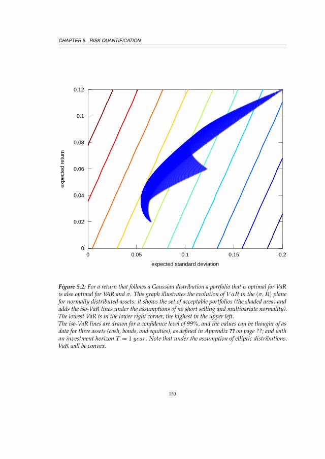
Figure 5.2: For a return that follows a Gaussian distribution a portfolio that is optimal for VaRis also optimal for VAR and σ. This graph illustrates the evolution of V aR in the (σ,R) planefor normally distributed assets: it shows the set of acceptable portfolios (the shaded area) andadds the iso-VaR lines under the assumptions of no short selling and multivariate normality).The lowest VaR is in the lower right corner, the highest in the upper left.The iso-VaR lines are drawn for a confidence level of 99%, and the values can be thought of asdata for three assets (cash, bonds, and equities), as defined in Appendix ?? on page ??; and withan investment horizon T = 1 year. Note that under the assumption of elliptic distributions,VaR will be convex.

150


-100

-80

-60

-40

-20

0

20

0 0.01 0.02 0.03 0.04 0.05

prof

it in

vest

or B

quantile

-100

-80

-60

-40

-20

0

20

0 0.01 0.02 0.03 0.04 0.05

prof

it in

vest

or A

0

0.005

0.01

0.015

0.02

-100 -80 -60 -40 -20 0 20

cdf i

nves

tor B

profit

0

0.005

0.01

0.015

0.02

-100 -80 -60 -40 -20 0 20

cdf i

nves

tor A

Figure 5.3: This figure shows the quantile function for Examples 5.1.1 and 5.1.2 in the twotop graphs; and the cumulative distribution function (cdf) in the two bottom graphs. Theprobability level of 0.01 returns a zero VaR in the non-diversified case (investor A), whereas inthe diversified case (investor B) the VaR is 50e. Note that even investor B has a probability of0.000049 of losing 100e.

151


Figure 5.4: The six graphs show the cdf for increasing numbers of bonds in portfolios—asdefined in 5.1.1 and 5.1.2. With this presentation, we can see what happens with the VaR: itsuffices to study the behaviour of the 0.01-quantile. This quantile corresponds to a value of thecdf of 0.01 (Note that the scale on the y-axis is logarithmic, and that the value of interest willbe 10−1). We notice that for one bond, the 0.01-quantile (and hence VaR) equal −5%. In thesecond graph, it is clear that the VaR is −47.5%. Increasing the number of bonds further, wenotice that the VaR will decrease slowly, but that when another step passes the 0.01 mark onthe y-axis, then VaR will make a jump upwards!

152


Figure 5.5: ESα and V aRα are shown as a function of α, for the case where we have onebond—defined in 5.1.1. If one believes that VaR is a reasonable risk measure, then one mustaccept the fact that the risk drops from 100% to −5% when the confidence interval passesfrom (1 − 0.006999999) to (1 − 0.007). This is a strong argument for stating that VaR isnot internally coherent. It is very reassuring that ES is continuous in α, and that hence smallvariations in confidence level will result in small variations in risk.

153


Figure 5.6: ES0.01 and V aR0.01 are shown as a function of the number of bonds in theportfolio, as defined in 5.1.1 and 5.1.2. Note that VaR displays a false minimum for 1, 21 and64 bonds.

154


Figure 5.7: The efficient frontier for ES0.01 and V aR0.01 are shown as a function of thenumber of bonds in the portfolio, as defined in 5.1.1 and 5.1.2. (The numbers on the plot are thenumbers of bonds in the portfolio). Note that VaR displays a false minimum for 1 bond and for21 bonds. ES, on the contrary, will systematically decrease as diversification increases; VaRbehaves erratically as a function of diversification.This is, of course, another view of the previous graph (Figure 5.6 on the preceding page).

155


means that VaR can counteract diversification11 Mathematicians would callthis “VaR is not sub-additive” (see De Brouwer (2012) and De Brouwer (2014)for example) or “not convex”. This actually means that in any logical andcoherent definition of “risk” VaR is not to be considered as a risk measure. It isa quantile and in a parallel universe where risks follow a Gaussian distribution,one can indeed use it as a risk measure for those risks, but that is not ouruniverse and not project finance.

Many other problems with VaR have been reported:

• Danıelsson (2002) finds that “for regulatory use, VaR may give mislead-ing information about risk, and in some cases may actually increase bothidiosyncratic and systemic risk”.

• Another aspect is that convexity of the risk surface is a consequence ofsub-additivity and positive homogeneity (see Acerbi et al. 2001).

• Yamai & Yoshiba (2002b) find empirical evidence that using VaR inpractice as a risk measure can be dangerous, because of the fact that VaRis not sub-additive and does neglect the form of the distributions beyondthe VaR level. However, they also stress that Expected Shortfall (thecoherent alternative to VaR) is sensitive to the stability of the parametersof the distribution of the tail risk.

• The same authors use simulation-based multivariate extreme value dis-tributions (Yamai & Yoshiba 2002a) to model markets under stress, andfind that both VaR and ES may underestimate the tail risk, and that “EShas less of a problem in disregarding the fat tail and the tail dependencethan VaR does”.

5.1.3 Expected Shortfall (ES)

In Search of a Simple Coherent Risk Measure

In their seminal paper “Thinking Coherently” in (1997) Artzner, et al. proposeda set of axioms that a risk measure should comply with. It was compellingand intuitive, but there followed an impasse of a few years because therewas no known risk measure that could practically be used and that would becoherent. The water between practitioners (bankers, asset managers, insurance

11This is one of the reasons why focus on VaR (as in Basel II for example) can be very dangerous.Lehman Brothers was always reporting good VaR numbers, but went bankrupt. VaR in essenceignores the tail of the distribution, discards all the information about the worst outcomes: that isnot what a risk measure should do.

156


companies, and regulators) and academics was suddenly very deep. Virtuallyall practitioners adopted VaR, probably because of its simplicity, wide applica-bility to all different kinds of assets and liabilities, and its being sufficientlyuniversal to be applied to many different risks and asssets on a bank’s balancesheet. However, the afore mentioned paper had put forward four axioms thatwere well in line with what one would expect from a risk measure; yet VaRdid not fulfil these axioms, and hence was not a coherent risk measure.

Because VaR violates the axioms of coherence, it can and will produceincoherent results. VaR calculations can result in lower VaR numbers formore risky portfolios, as has been shown in Example 5.1.1 on page 149 andExample 5.1.2 on page 149. VaR could lead to situations where people believethey have risk under control, but they are actually building a time bomb.Nonetheless, for a few years there was no alternative, until Pflug in (2000)proved that Expected Shortfall fulfilled all the criteria of coherence.

it appears that in order to get a coherent risk measure, one needs to answera closely related question: “What is the expected loss in the 100α% worstcases?”.12 The answer to that question leads to the concept known as ExpectedShortfall.13

Characterisation for ES for Discrete Distributions

By using the average of the 100α% lowest results of a number of realizations{Pi}{i=1,...,N} of the stochastic variable P , one has finally a coherent riskmeasure, known as expected shortfall (henceforth ES) or conditional value atrisk.

Let us denote the sorted values of the n-tuple (P1,P2, . . . ,PN ) as(P1:N ,P2:N , . . . ,PN :N ); and let us approximate the number of the 100α%lowest results by

n = max{j|j ≤ αN, j ∈ N} = int(Nα)

Remark 5.1.1. Any other form of rounding or truncating of Nα is acceptable,and would also lead to (another) coherent risk measure.

12One could even argue that the minimal loss in the 100α% worst cases is not the most relevantinformation; the worst loss or the expected loss provide much more relevant information for therisk-averse investor.

13In the literature, Expected Shortfall (ES) is also referred to as CVaR (Conditional Value at Risk),Average Shortfall, AVaR (Average VaR), ETL (Expected Tail Risk); additionally, for continuousdistributions, TCE (Tail Conditional Expectation) is the same. For mor deeper information andproof we refer to (De Brouwer 2012).

157


Hence we can use the following natural estimator for q(α)N (P)

qN (α;P) = Pn:N (5.14)

Then the natural estimator for the expected loss in the 100α% (or the 100α%Expected Shortfall) worst cases is given by:

Definition 5.1.8 (Expected Shortfall (ES)). Let Pi:N be the observationsof stochastic variable P ordered from low to high and, n the number oflowest observations that correspond to the 100α% lowest observations,Pn:N be the estimator for qN (α;P), then the Expected Shortfall is theexpected loss in the 100α% worst cases of the stochastic variable P repre-senting the absolute returns.

ES(α)N (P) := −∑ni=1 Pi:Nn

= - (average of the worst 100α% realizations)

For the technical details we refer to De Brouwer (2012) (pages 122 to 128),but the definition A.2.3 can be rewritten with the aid of left-generalized inversefunction F←P of the cumulative distribution function FP(x), which is definedas;

F←P (p) := inf{p|FP(p) ≥ p}. (5.15)

We note that for continuous distributions F←P (p) = QP(p) and we are readyto rewrite the characterization of ES.

Definition 5.1.9 (Characterisation of ES for continuous profits). Let Pbe a continuous stochastic profit variable –in nominal terms– with left-generalized inverse function F←P , quantile function QP(p), and proba-bility density function fP , and α ∈ [0, 1], then the α expected shortfall

158


(ES(α)(P)) can also be characterized by

ES(α)(P) = − 1

α

∫ α

0

F←P (p) dp (5.16)

= − 1

α

∫ α

0

Q(p) dp (5.17)

= − 1

α

∫ α

0

V aR(α)(P)(p) dp (5.18)

= − 1

α

∫ QP(α)

−∞fP(p) dp (5.19)

The equivalence with Definition 5.19 is intuitively understandable; andEquation 5.18 illustrates the alternative name “average VaR” or “ConditionalVaR”.

This characterization makes immediately clear that ES is continuous inα. This is a very important property, since otherwise the risk measure of αand α + ∆ can be very different, even for a very small ∆. This immediatelyillustrates how one of the problems with VaR is solved by ES.

Acerbi et al. (2001) conclude that ES has the following advantages: ES is

• universal: it can be applied to any financial instrument and to any formof underlying risk,

• complete: it can produce a unique global assessment that aggregatesdifferent forms of risk,

• simple: it is the answer to a very natural question and has a clear inter-pretation.

Note. The formulae in the previous example are also valid for other definitionsof return. Indeed, one can also define the expected shortfall as a percentagevia ES(R). However, note that this will not lead to a coherent risk measure.For example, ES(R) would not be positively homogeneous. A solution mightbe to use V0ES(R), which is essentially the same as P .

Note. A natural way to extend the concept of ES for α → 0 is to use theworst-case outcome for X :

ES(0) := −ess.inf{X}

159


0

0.5

1

1.5

2

2.5

3

3.5

0 0.2 0.4 0.6 0.8 1

ES

alph

a

α

0

0.5

1

1.5

2

2.5

0 0.2 0.4 0.6 0.8 1

ES

0.05

σ

Figure 5.8: This figure shows how ES behaves as a function of α (upper graph) and as afunction of σ (lower graph) for the Gaussian distribution: ES is linear in σ. Hence for thenormal distribution, the same portfolios will be efficient for both mean-ES optimization as formean-variance optimization.

160


where ess.inf{X} is the essential infimum14.

ES is a coherent risk measure

For a formal proof that ES is a coherent risk measure we refer to Pflug (2000),Acerbi & Tasche (2002a) or De Brouwer (2012).16 In this book we will limitourselves discussing the impact and advantages of using a coherent riskmeasure.

In Figure 5.9 on the next page we illustrate intuitively the critical differencebetween VaR (no “risk measure”, or at least not a “coherent” risk measure)and ES (a coherent risk measure). The plots show to hypothetical probabilitydensity functions (pdfs): on the left side one that follows a Gaussian distri-bution and on the right side one that does not follow a Gaussian at all. Thedistribution on the right side is similar to a Gaussian above a certain level, butthe extreme risks (tail-risk) is very different: in stead of being very confined–as so typical for a Gaussian pdf– one will notice that losses of -300 are possible(on the left this is rather excluded, as the Gaussian pdf converges very fast tozero).

In that example VaR does not see a difference! However, ES will find animportant difference. The standard deviation, will also increase and –at least–indicated that both pdfs are not the same.17

14The essential infimum is defined as

ess.inf(X) := sup{a ∈ R : µ ({x : f(x) > a}) = 0}

and is thereby an extension of the concept of infimum,15 in the sense that if the infimum does notexist, the essential infimum may still exist, but it disregards the values of the set with measurezero. In other words, almost everywhere the essential infimum is the infimum, except on a subsetwith measure zero.

16Further, via the theory of “spectral risk measures” or “distortion risk measures” (both ex-plained in De Brouwer (2012)) one can show that ES is actually the most simple coherent riskmeasure.

17To illustrate how absurd VAR (or σ) would be as a risk measure, it is sufficient to usedistribution functions that are exactly the same: for example a normal distribution function withaverage £ 100 and standard deviation £ 2 for project A, and in project B everything is the same,except for the condition that the Sponsor will take first £ 3 out of the SPV before the SPV pays thebank. In that case the return of the project keeps the same distribution, but simply is moved to theleft, seriously increasing the probability that the bank will not get her investment back. In thiscase ES and VaR (most probably) will see a difference, but VAR will fail.

161


Figure 5.9: In this figure we show left a confined distribution (eg. a Gaussian distribution), onthe right a distribution that is largely the same, except for the extreme risks. In both cases atypical return is around zero with only small deviations (say between £ 4 miln and £ 4 mln)but on the right side there is a small probability to have large losses (say a 2% probability thatthe loss is around £ 350 mln.). VaR will see no difference, VAR might notice it a little but onlya coherent risk measure –such as ES– is bound to see the difference. So, a bank that is usingonly VaR will be motivated to take the large loss on board because the potential returns will behigh –the market is not blind for the risk, onlyl the one using only VaR– and this high potentialreturn will not be offset by higher capital demand because VaR will not see the risk.

162

5.2. RISK MODELING

5.2 Risk Modeling

Now that we have shown that there exists at least one risk measure that isworth this title, the next problem is how to estimate this value (or any otherparameter that we deem relevant). A large infrastructure project is typicallyone that is unique in many aspects. Even if it is a project that has been donebefore, it will be unique in that period in that geographical space. So wemust be careful using the law of large numbers and convergence to a levydistribution under convolution –as Bouchaud & Potters (1997) warn us. Firstof all: there are no large numbers (even the largest bank will only have alimited number of projects), and hence there are not too much convolutionsto be made.18 Secondly it is very hard to find relevant(!) historic data. This isnot only because there aren’t so many similar projects, but most importantlyall large projects will be unique. Even building twice the same nuclear powerstation in China will be a unique challenge because the few decades differencemake in the second case the technology better known, but some skills harderto find, more or less administration and regulation, maybe there is a globaleconomic crisis that separates the projects, etc.

So, in order to get an idea on the possible outcomes of the project oneneeds at least a zero hypothesis: this is called “the business plan”. Theseare the official numbers put forward by the SPV that seeks the loan. It willbe a detailed plan of cash-flows leading to construction and then incomingcash-flows from the exploitation of the project. Any investor can see (from hispoint of view of course) what each of the following parameters is:

• time to profit: how long does it take before the investment (SPV) makesprofit

• time to break even: how long does it take before the investments equalthe income

• NPV: the sum of all discounted cash flows NPV =∑Nt=0

CFt(1+r)t

• IRR: internal rate of return or the discount rate that makes the IRRzero. In case the investments are just one up-front investment, then itequals the discount rate at which the present value of all future cashflow is equal to the initial investment or in other words the rate atwhich an investment “breaks even”. Still otherwise stated, the IRR of aninvestment is the discount rate at which the net present value of negative

18The relevance lies herin that the convergence to a Levy distribution or Gaussian in most casesis slow, and actually never (unless in the mathematical case of infinity) work for the tails.

163


cash flows of the investment equals the net present value of the positivecash flows.

• etc.

This can be done in a simple spreadsheet such as LibreOffice Calc19. Thissimple approach already gives a good approximation of what is to be expected.

Now, assume that we consider IRR as the most relevant parameter andfind a results of 14%. Is that a good or a bad result? In order to answer thatquestion one has to compare the return with the risk. But in order to calculatethe risk (for example ES) it is necessary to have a good idea how the returnsare distributed. That is not so straightforward for large projects that are allquite unique.

The best method is of course starting from the underlying distributionscalculate the distribution of the end-result. In practice, however this is notpossible for project finance: distributions are unknown, non-linear interactionsare possible, some events depends on others, etc.

The first, most simple, but most limited method is “stress testing”.

5.2.1 Stress Testing

In order to gain some insight in how robust a certain result of our businessplan is or what bad cases can be expected a simple stress test can answer thatquestion.

A simple example could be: allow the price of certain raw materials tofluctuate (simply test a few possibilities), then do the same with labour prices,allow the effect of a strike, an earthquake, fluctuations in exchange rates, oneof the lenders that gets into problems, we have to halt digging because westumbled upon a site of historic importance, etc.

Soon, one of the problems with stress testing become obvious: it becomesbewildering how much possibilities there are, it is impossible to say which ismore probable that the other, etc. The answer to that shortcoming is simplyto restrict stress testing to what it does best: explore extreme risks –withoutknowing how likely it is. So for example assume that an earthquake destroysa lot of the half-build site, killed a few people causing a strike, the currency toplunge and the domestic bank in the syndicate gets into problems because ofthat. Then we have just one scenario, something that we can calculate withyour spreadsheet and that gives us a “worst case scenario”.

19LibreOffice is community-driven and developed software, and is a project of the not-for-profitorganization, The Document Foundation. See: http://www.libreoffice.org/.

164

http://www.libreoffice.org/

5.2. RISK MODELING

The relevance for each lender is that he should ask the question “can Iafford to loose that much”, if the answer is “no”, then the lender should seekanother partner in the syndicate, the sponsor another partner for the SHA, etc.Failing to do so is planning for the next Global Meltdown to start.

In order to do that in practice, a spreadsheet might stillbe sufficient, how-ever, it might be advisable to follow a few simple rules to keep it organized.For example:

• Use different tabs (sheets) for (a) assumptions, (b) costs, (c) income, (d)P&L and (e) ratios.

• Make sure that each sheet has the same columns (the columns should besomething like A, B, C and D hold titles, E is 2015-Jan, F is 2015-Feb, etc.

• Use different colours to make the different function of each cell clear: forexample pale yellow for an input cell, no background for the result of acalculation, etc.

• Avoid –where possible– obscure formulae that are difficult to read forhumans

• Do use as much as possible underlying programming language (VisualBasic for example) and never ever use marcos (macros are very difficultto read by other humans, not re-useable, slow and confusing).

• Keep different version, have frequent team-meetings when working onone file and agree who will modify what.

Following these simple rules will help you to make rather complex modelsin the simple spreadsheet that a modern computer offers. The downside ofa stress test is that it does not tell how likely a certain result is. To get thatessential insight it is necessary to use other techniques.

If you find that the spreadsheet becomes difficult to read or slow we suggestto have a look at the alternatives presented in Chapter 5.2.3 on page 167

5.2.2 Monte Carlo Simulations

A Monte-Carlo simulation can simply be understood as hundreds of thousandsof Stress Tests run by an automated machine so that it becomes possible toget an idea about how probable certain outcomes are. This is of course onlypossible if we are able to say something sensible about the underlying riskfactors.

165


With “something sensible” we mean that we know something about thelikelihood of something to happen. We might not know the exact distribution,but at least some probability. For example we might expect an earthquake offorce 4 to happen once in thousand years. This simple number is far less thanknowing the probability density function, but it can already work.

In that case we would have a 0.000083 probability each month that suchearthquake would occur. However if it occurs, then the knock-on effects willbe significant for the project: damage, delays, other problems in the regionneeding attention, etc. It is here that the limitations of a spreadsheet becomeall too clear. It becomes impossible to model correctly the effect of such events,not only because of the interdependence with other parameters, but also intime. If such event occurred, then is it more or less likely to happen again?Some effects will be immediate (such as if the currency drops 20% with respectto the currency that we use to pay a certain material or service, then thatservice or material is immediately more expensive). This can still be modeledin a spreadsheet, but in the realistic case with the earthquake one must takeinto account a whole different scenario for the rest of the project and thatbecomes almost impossible and at least very convoluted.

The alternative is to use a programming language that allows us to modelanything. Best suited for large projects are languages that allow for someobject oriented code. We can use the features of an object oriented program-ming language to represent actors and input in our project. For example theengineering company can be one “object” and it will decide to hedge currencyrisk if the exchange rate hits a certain barrier, etc.

This allows us to model dependencies such as in our example with theearthquake. If the earthquake happened, then other objects can “see” thatand react accordingly, the exchange rate (also an object) will switch regime (ie.draw its result from a different distribution), the workers can see the impact ofthe safety conditions and consider a strike with a given probability, etc. Thisway of working is not so far removed from the way modern computer gameswork.

Good examples of programming languages that allow vast amounts ofcomplex calculations are C++ and R. The high level of abstraction offeredby object oriented programming languages allows the programmer to createobjects that can interact with each other and their environment. For examplethe Engineering Company can be such object. That object can be instructed toemploy more workers when a delay threatens to happen but up to the limit thatthe extra costs are offset by the potential penalties. As the simulation then runs,market parameters change and events happen according to their probability ofoccurrence and each object will then interact in a pre-programmed or stochastic

166

5.2. RISK MODELING

way.This allows very complex behaviour and dependencies to be modeled, yet

everything will be in a logical place and any other programmer can read it as abook. On top of that there are good free solutions to create free a professionaldocumentation set. For example Doxygen (see http://www.doxygen.org)is free and able to create both an interactive website as well as a LATEX20 bookfor the documentation, that details each class, function, handle, property,etc. Code written in such way and documented properly is not only easy tomaintain, but also straightforward to audit and as a bonus one gets the speedof C++.

5.2.3 Beyond the Monte Carlo Simulation

Now that we have a good idea how the distribution of the results will look like,we can use this distribution to calculate the relevant risk parameters. In manycases the “historic” distribution that we got by our Monte Carlo simulationwill be usable, however for large and complex projects the distribution mightnot be very smooth. If we believe that this is a sign of the limited number ofsimulations, then we can try to apply a kernel estimation in order to obtain asmoother results that yield more robust risk parameters.

The technique of kernel density estimation (KDE) could be helpful forall distributions that are estimated from a histogram. As an alternative toparametric estimation where one infers a certain distribution it avoids thestrong assumption that the data indeed follows that given distribution. Note aKDE can be used also for any input parameter where the distribution used isbased on observations.

Of course one can choose a standard distribution if the we have reasonsto assume that this would be a good approximation. However, choosing anon-parametric kernel density estimation, has the advantage of avoiding anyassumptions about the distribution, and on top of that:

• it is well documented in the case of expected shortfall—(e.g. Scaillet 2004,Chen 2008, Scaillet 2005, Bertsimas, et al. 2004)

• there is research on its sensitivity with respect to the portfolio composi-tion, w—(see Scaillet 2004, Fermanian & Scaillet 2005)

20LaTeX is a high-quality typesetting system; it includes a large set of features designed forthe production of technical and scientific documentation. LATEXis the de-facto standard for thecommunication and publication of scientific documents. LATEXis available as free software in therepositories of your distribution and at http://www.latex-project.org/.

167

http://www.doxygen.org

http://www.latex-project.org/


Using a non-parametric kernel density estimation, however, requires onearbitrary parameter: “the bandwidth”. The bandwidth is a parameter thatis related to the level to which the data sample is representative of the realunderlying distribution. If one makes a too-small choice of this parameter, oneforces the estimated distribution function, fest, to stick too much to the data,and there is too little of a smoothing effect. If, on the other hand, the parameteris insufficiently restrictive, then fest will be smeared out over an area that istoo large.21 More information on bandwidth selection can be found in Jones,et al. (1996b).

Of course, one can ask if it is necessary at all use a kernel estimation insteadof working with the histogram obtained from the data. Using the histogramas pdf has a few disadvantages:

• it is not smooth (this observation tells us that the use of histograms issimilar to noticing that the dataset is imperfect and not doing anythingabout it),

• it depends on the end points of the bins that are used (changing the endpoints can dramatically change the shape of the histograms),

• it depends on the width of the bins (this parameter can also change theshape of the histogram),

• it introduces two arbitrary parameters: the start point of the first bin,and the width of the bins.

An answer to the first two points (and half of the last point) is to use a kerneldensity estimation. In that procedure, a certain function is centred around eachdata point (for example, an indicator function, a Gaussian distribution, the topof a cosine, etc.), these functions then are summed to form the estimator of thedensity function. The kernel density estimation is currently the most popularmethod for non-parametric density estimation (see e.g. the following booksScott 2015, Wand & Jones 1994, Simonoff 2012)

This method consists in estimating the real (but unknown) density functionf(x) with

fest(x;h) =1

N

N∑n=1

Kh(x− xn) =1

Nh

N∑n=1

K

(x− xnh

)(5.20)

where K is the kernel21Note that we do not use the usual notation for the estimated distribution density function, f ,

because we have reserved that notation for the Fourier transform.

168

5.2. RISK MODELING

Definition 5.2.1 (Kernel). A kernel is a function K(x) : R 7→ R+ thatsatisfies the following conditions.

+∞∫−∞

K(u) du = 1

∀u ∈ R : K(u) = K(−u)

If K is a kernel, then also K∗(u) := 1hK

(uh

)(with h > 0) is a kernel. This

introduces an elegant way to use h as a smoothing parameter, often called “thebandwidth”.

This method was hinted by Rosenblatt et al. (1956) and further developedin its actual form by Parzen (1962). The method is thus also known as the“Parzen-Rozenblatt window method”

The Epachenikov kernel (see Epanechnikov 1969) is optimal in a minimumvariance sense, however it has been shown by Wand & Jones (1994) that theloss of efficiency is minimal for the Gaussian, triangular, biweight, triweight,and uniform kernels.

We believe it if we believe that an underlying pdf exists, kernel densityestimations have a few distinct advantages over histograms: they can offer asmooth density function for an appropriate kernel and bandwidth, and theendpoints of the bins are no longer an arbitrary parameter (and hence wehave one arbitrary parameter less, but still the bandwith remains an arbitraryparameter).

We also note that Scott (1979) proves the statistical inferiority of histogramscompared to a Gaussian kernel with the aid of Monte Carlo simulations. Thisinferiority of histograms is measured in the L2 norm, usually referred to asthe “mean integrated squared error” (henceforth MISE), which is defined asfollows.

MISE(h) = E

+∞∫−∞

{fest(x;h)− f(x)}2 dx

(5.21)

A variant of this, the AMISE (asymptotic version), can also be defined,and this allows us to write an explicit form of the optimal bandwidth, h.Both measures have their relevance in testing a specific bandwidth selectionmethod, for example. However, for our purpose these formulae cannot be

169


Figure 5.10: Left, the Epachenikov kernel, KEh (x) = 3

4h

(1−

(uh

)2)1{|u/h|≤1} for h = 1;

and right the Gaussian kernel, KGh (u) = 1√

2Πhe−u

2

h2 for h = 0.5.

used since they contain the unknown density function f(x). Many alternativeshave been proposed and many comparative studies have been carried out.A first heuristic was called “cross validation selectors” (see Rudemo 1982,Bowman 1984, Hall, et al. 1992). Sheather & Jones (1991) developed “plug-inselectors” and showed their theoretical and practical advantages over existingmethods, as well as their reliable performance. A good overview is in Jones,et al. (1996a).

Conclusion Kernel Estimation is a widely accepted and used method thathas many advantages. However, it introduces the arbitrary choice of band-width and of type of kernel. However, we note a novel method that automatesthis selection without the use of arbitrary normal reference rules (see Botev,et al. 2010). We also note that it is blind to specific aspects, such as the bound-edness of the domain of values (e.g. prices cannot become negative). Thereforethe method has to be used with care, and preferably on non-bounded data(e.g. log-returns).

170

5.2. RISK MODELING

Figure 5.11: As illustration on how the Epachenikov Kernels Estimation works, we present inthe upper graph the histogram of the annual inflation corrected returns of standard asset classes.The lower graph offers a view on what a non-parametric kernel density estimation on those datacan do.

171

Chapter6Conclusion

In this part of the book we proposed that risk management is not only anessential part project financing, but that it is actually the reason why projectfinance exists. Therefore good risk management is key for all parties involved,each party has its own particular risks. What can be a risk mitigation for oneparty can be a new risk for another party. We proposed that risk managementshould follow a “risk cycle” and that the risk manager should continue to gothrough that cycle and continue to mitigate and improve the project.

Figure 2.1 on page 118 visualizes this idea –that the risk manager andhis/her team should continuously cycle through the different aspects. Forexample the risk manager could decide to make weekly minor updates andmonthly review all aspects involved (including the models, etc.). But evenmore essential than following a certain procedure is how practically orientedthe risk manager is and how well he/she understands the big picture: thewhole project. Once a risk is identified and assessed to be important, thenhe/she should go out and make sure that an appropriate mitigation is in place.In order to do so the risk manager will have to be involved in many decisions,be close to everyone and be a trusted partner for CEO and workers.

This section provided you with

1. a checklist of types of risks to look after in LRL (see Chapter 3 onpage 121),

2. a simple way of visualizing, prioritizing and following up risks with a“risk matrix” (see Chapter 4 on page 133)

CHAPTER 6. CONCLUSION

3. and all the mathematical tools to fill out this risk matrix (see Chapter 5 onpage 137) — and if you would have skipped this part: the key messageis that one should not ignore risk because they are very improbable.1

The reader will notice that there is no section on “risk mitigation”. Thisis because risk mitigation is very specific in each situation and can only beassessed taking into account all specific human, engineering, political andenvironmental aspects. Therefore each risk mitigation will be highly specificto each project, company and even for each individual involved.

This section about risk management should give the risk manager a solidset of tools and a framework to do his/her job and communicate about it,but relevant practical experience remains quintessential. The most importantaspect of risk management remains the way the risk manager (a) gains trust inthe company in order to get all relevant information and (b) how he/she usesthis information to mitigate risk before they realize. The risk manager shouldstrive to be a trusted consultant to each person and team in the company andalways keep the big picture in mind.

Though it is essential in the thinking about risk that there is nor freeenterprise nor gain without risk. However there should be a healthy trade-offbetween risk and return: for a higher risk one should be able to expect a higherreturn. If a company were to plot its projects or loans in a risk-return graph,then it should look similar to the efficient frontier as presented in (considerthe upper boundary of the plot in Figure 5.1 on page 141: an increasing curve).A company should within its risk appetite take only risks on board if thepotential return is high enough.

While it is possible to make a some risks disappear (as eliminating explo-

1This remark refers to the fact that in the VaR is still used in regulations despite the fact thatit totally ignores large-but-improbable risks. It seems remarkable that a risk measure that hasproven to be very dangerous such as Value at Risk as it accompanied Lehman Brothers to its graveis still used. This seems to be similar to finding that it is hard to pick up mercury with a fork andthen pass a regulation that forces bankers to use bigger forks. Arguably, a coherent risk measure–such as Expected Shortfall– might have been a small step in the right direction. However oncemore one would have to conclude that large infrastructure projects are always so unique that itbecomes very hard to calculate any risk measure at all – and note that a coherent risk measurenecessary needs more assumptions and/or knowledge about the tail of the distribution than VaRfor example.

Indeed using a coherent risk measure in legislation is in our opinion only a “small step”: wemean that a legislation such as Basel III creates inherently systemic risk and that this will not besolved by using a different risk measure. The problem is that a regulation that forces everyoneto calculate in the same way and use the same risk limits is bound to create problems. Imaginethat bank A hits its risk limit and has to sell investment X. That will put the price of investment Xunder pressure and that might in its turn push bank B over its limit, forcing it to sell X. This mightlead to non-linear feedback system (in finance typically referred to as “systemic risk”.

174

sion risk by closing a bottle filled with methane gas), no risk management isable to eliminate all risk of an infrastructure project. Recent years have seenincreasing pressure on banks to become more safe organizations (Basel II andBasel III regulation for example — with Basel III especially tough on long termlending that is so much needed by infrastructure projects). Unfortunately theseregulations make it difficult for banks to lend long-term and hence banks areless and less able to play their role in economic growth and project financing.

Probably the biggest risk that our society faces –especially in Europe– isthe lack of economic growth induced by the de-leveraging of banks by andregulations such as Basel III. Perversely, the fear of the dilemma whetheror not to bail out a bank has put the “taxpayer” directly liable for failingprojects via Export Credit Agencies and the European Long-Term InvestmentFunds (ELTIFs).2 Economic growth needs infrastructure projects and these arerisky, that risk will never disappear: it can only be pushed to other parties orthere will be less or no projects. If banks are not allowed to take on the risks,then other institutions will have to take that risk, otherwise the economy willstagnate.

It is unfortunate that humans only build traffic lights after accidents andthat no-one ever has the courage to challenge existing lights. Regulators andlaw-makers only tighten regulation after a crisis . . . while the economy actuallyneeds a much looser regime in order to recover. Maybe the availability bias–that causes short-term thinking– should be overcome and we should tightenregulation when the economy is doing great and –equally important– loosenregulation when economic growth is slow. This could even be built in into theregulation itself.

Will you have the courage and the long term view to start this?

2These –government owned– agencies tend to take over more and long term lending frombanks. So when the project fails, the government is directly on the hook for the losses.

175

Part II

Addenda

AppendixACoherent Risk Measures

Note. This section is inspired on De Brouwer (2014).

A.1 Introduction

Financial institutions in general and banks in particular are –till now– thevery heart of our free market economy. Banks help to put capital to use:they redistribute money from those who have cash but ran out of ideas orenergy to those that have ideas and energy but insufficient cash. However, theGlobal Meltdown of 2008 has shown that they can be fragile. How was all thatpossible? How should one try to keep the risks in check? These questions arehardly discussed and law-makers simply assume that by doing more of whatthey did before it should all work out . . . till next time.

The essence of all commercial companies is to take risks and get a marketpremium in return. This also holds for banks and in a simple approach a bankcan hold deposits (their liabilities) and give credits on the other side of theirbalance sheet (the bank’s assets). Of course they will leverage this game inorder to make more profit. So, the simple answer cannot be to make banksrisk-less, because that would stall the economy and make them useless: risksare necessary but how can we control them?

Bernoulli (1738) recognized that the risk averse investor –and when banksinvest in another legal or private person’s debt, they are investors– shouldseek to diversify, Fisher (1906) proposed variance as a measure for economicrisk, and Markovitz’ PhD supervisor Marschak (1938) suggested to use mean

APPENDIX A. COHERENT RISK MEASURES

and variance as parameters in utility (for consumption of commodities). How-ever we had to wait till Markowitz (1952) for the first explicit quantificationand identification of investment risk, when he proposed his mean-variancecriterion. After almost 60 years his method is often used by practitioners andremains a reference for scholars (e.g Rubinstein 2002). Markowitz used in hisseminal paper of 1952 variance as risk measure. He did not discus in thatpaper the choice for variance but argued that the mean-variance criterion wasbetter than simply chasing return because it stimulated diversification: a wiseand fundamental argument!

Now –70 years later and a few crisis wiser– the race is on to regulate Banksmore and more strict in order to avoid a repetition of the meltdown in 2008.For example a series of “Basel” regulations try to de-leverage banks. Theregulation tries to achieve this by using one risk framework and require banksstay within the limits set by that framework. This risk framework is based onValue at Risk (VaR) as a risk measure.1 We will define it later, but first take astep back and look what scientific literature has available that one could haveused instead.

A.2 Definitions

A.2.1 Coherent Risk Measures

Considering the question of how financial risk could be described, Artzner,et al. (1997) proposed the following set of axioms2:

Axiom A.2.1 (Coherent Risk Measure). A function ρ : V 7→ R (where Vis the set of real-valued stochastic variables) is called a coherent risk measureif and only if it is

1. monotonous: ∀X,Y ∈ V : X ≤ Y ⇒ ρ(X) ≥ ρ(Y )If a portfolio Y has always better results than portfolio X, then itsrisk is less.

1Enforcing one risk framework is risky, because it means that if things go wrong despite therisk framework (and statistically that is bound to happen) then many banks will be in the samedire streets for the same reason. This in itself works “systemic” and is dangerous. We do not focuson this discussion, but focus on the risk framework itself.

2For a profound elaboration and the proof that VaR is incoherent, please refer to Artzner, et al.(1999).

180

A.2. DEFINITIONS

2. sub-additive: ∀X,Y,X + Y ∈ V : ρ(X + Y ) ≤ ρ(X) + ρ(Y )Diversification reduces risk: the risk of a portfolio cannot be worsethan that of any of its constituents separately.

3. positively homogeneous: ∀a > 0 and∀X, aX ∈ V : ρ(aX) = aρ(X)Investing a times more money increases the risk a times.

4. translational invariant: ∀c > 0 and ∀X ∈ V : ρ(X + c) = ρ(X)− cAdding an amount c in cash to the portfolio reduces the risk with c.

These axioms are congruent with what one intuitively understands as“risk” in a financial context. Axiom two for example states that diversificationreduces risk. Indeed when one owns two assets, the outcome is in the worstcase the result of the two worst case scenarios. In all other cases the outcome ofthe diversified portfolio is better. This is so fundamental in our thinking aboutfinancial risk that Artzner et al. elected this as an axiom for coherence andthat Markowitz (1952) considered this aspect as the key test for his new meanvariance criterion. Some authors, such as Acerbi & Tasche (2002a) consideronly risk measures that are coherent in this sense and refuse to label othermeasures, such as Value at Risk (VaR henceforth), variance (VAR henceforth)and standard deviation, as “risk measure”.

An important footnote is that these axioms are only realistic when marketsare liquid and when the investor would never be in a position to influenceprice. This phenomenon –of limited validity– is not an argument against theaxioms. This is so with most axioms such as for example the Euclidean axiomsof geometry. This geometry generally work fine, but fails to describe reality inthe presence of large masses—where one needs the theory of General Relativity(see Einstein 1916). Also, similar to the Euclidean axioms, this does not meanthat this is the only set of possible axioms. For example it is possible to developinternally coherent geometries with different axioms, such as Lobachevskyand Bolyai’s geometry on the surface of a pseudo-sphere, or the geometry ona sphere, developed by Riemann. While none of these sets of axioms can bewrong or right, only the Euclidean geometry makes sense for applications suchas building a house or a printing a book. In the same way we will illustratethat Artzner et al.’s set of axioms lead to a coherent representation of risk inliquid financial markets for investors who cannot influence price.

181


A.2.2 Variance (VAR)

Variance is defined as follows.

Definition A.2.1 (Variance (VAR)). LetX be a real-valued stochastic vari-able, its variance is then defined as:

V AR := E[(X − E[X])2] (A.1)

= E[X2]− (E[X])2 (A.2)

=

∫R

(x− µ)2 fX(x) dx (A.3)

with µ := E[X] =∫R x fX(x) dx

Note that since standard deviation is a monotonous function of VAR thatall the results in this paper that are obtained for VAR are also valid for standarddeviation.

A.2.3 Value at Risk (VaR)

First we define Value at Risk (VaR).

Definition A.2.2 (Value at Risk (VaR)). For the real-valued stochasticprofit variable, return (X), and a probability α ∈ [0, 1], the Value at Risk(VaR) is defined as

V aRα(X) := −qα(X)

with qα(X) the α-quantile of the stochastic variable X .

Note that in the rest of the paper we will assume a “profit variable” whendiscussing risks (in line with practice in banking and asset management asopposed to practice in insurance where one typically considers the distributionof the “loss variable”).

182

A.2. DEFINITIONS

Often this definition is worded as “the VaR, given a confidence intervalof (1− α), is that value so that there is a probability of α to have an outcomeworse than VaR.” In other words, the “α-VaR is the best outcome of the 100α%worst outcomes”.

A.2.4 Expected Shortfall (ES)

Quite probably VaR is so popular for its simplicity, ease of calculation, uni-versality, and seemingly (but deceivingly) ease of interpretation. VaR is theanswer to the simple question: “What is the lowest amount that one can expectto loose in the 100α% worst cases?”. Another advantage is that it is expressedin the same units as the portfolio, and hence can have some intuitive interpre-tation. In the years that followed Artzner et al. (1997)’s publication there wasno coherent alternative for VaR known that combined all of the advantagesthat made it so popular.

Pflug (2000) proved that the answer to the following simple and question:“What is the average amount of loss in the 100α% worst cases?” leads to acoherent risk measure. This risk measure goes by many names: ConditionalValue at Risk (CVaR), Expected Shortfall (ES), Average Value at Risk (AVaR),Expected Tail Risk (ETR). For continuous distributions it coincides with theTail Conditional Expectation (TCE). For non-continuous distributions TCE is,however, not the same as ES. For non-continuous distributions it can even benon sub-additive.

We will choose for the name Expected Shortfall (ES henceforth), as it seemsthe most clarifying and pure and define ES as follows.

Definition A.2.3 (Expected Shortfall (ES)). For a real-valued stochasticprofit variable, X (such as return), the Expected Shortfall is the expectedloss in the 100α% worst observations

ES(α)N (X) := −∑ni=1Xi:N

n= - (average of the worst 100α% realizations)

Where the index i:N refers to the index of the observations, after sort-ing from the worst to the best observations, and n is a number to bedetermined in function of α.

183


(Acerbi & Tasche 2002b) show that this is equivalent with;

Definition A.2.4 (Expected Shortfall).

ES(α)(X) := − 1

α

∫ α

0

F←(p) dp

with F←(p) := inf{x|F (x) ≥ p}, the left-generalized inverse of the cumu-lative distribution function of X . For continuous distributions one hasF←X (p) = qα(X).

This definition makes immediately clear that ES is continuous in α. This isa property that has conceptual importance, and is not possessed by VaR, forexample. Figure A.1 shows how counter-intuitive this makes VaR.

Corollary A.2.1. For continuous distributions, this definition can be written as

ES(α)(X) = − 1

α

∫ α

0

QX(p) dp (A.4)

withQ(p) the quantile function (or the inverse of the cumulative distribution function)

Which is then also equivalent to

ES(α)(X) = − 1

α

∫ qα(X)

0

xfX(x) dx

So, since 2000 we have a coherent alternative for VaR that has most of itsadvantages: simple interpretation, expressed in monetary unit of measurementand universality of use. However there is a drawback: ES is more difficultto estimate. Indeed, where VaR simply ignores tail of the distribution, ESwill take all worst outcomes into account. This makes ES more sensitiveto estimation errors in the tails of the distributions. However we note thatthere are many ways to simplify the calculations.3 Also note that for a givenprobability, ES is always higher or equal than VaR.

3For portfolio optimization and risk minimization we refer to (see for the fundamentals:Rockafellar & Uryasev 2000, Rockafellar & Uryasev 2002, Uryasev 2000, ?) and (for overviewsDe Brouwer 2012, Acerbi & Simonetti 2002, Strepparava 2009); for comonotonic approximations: (?,see)]vanduffel2005comonotonicity,vanduffel2008optimal,dhaene2007comonotonicity,dhaene2005comonotonic,vanduffel2005comparing.

184

A.2. DEFINITIONS

Figure A.1: The V aR0.01 and ES0.01 in function of α for one bond as defined in ExampleA.3.1. If one believes that VaR is reasonable, then it is reasonable to see the risk drop from 100%to −5% when the desired confidence level passes from (1− 0.0069999) to (1− 0.0070000). Itis reassuring that ES is continuous in α.

185


More importantly, one can consider the question if it is better to have a lessstable calculation or is it better to neglect the highest risks all together as in aVaR calculation. We believe that the answer to that question is obvious and infavour of ES.

A.2.5 Spectral Risk Measures

A simple and elegant proof for sub-additivity of ES for discrete distributionsis presented by (De Brouwer 2012) (pages 124 and 125). For continuousdistributions the proof is generally given via Distortion Risk Measures or viaSpectral Risk Measures. Both representations are equivalent.

In general, we can define spectral risk measures as follows.

Definition A.2.5 (Spectral Risk Measure). Let X be a stochastic variable,representing the return of a financial asset. Then we define the spectralmeasure of risk Mφ(X) with spectrum (or risk aversion function) φ(p) :[0, 1] 7→ R as:

Mφ(X) := −∫ 1

0

φ(p)F←X (p) dp

Example A.2.1. The spectrum or risk aversion function for the α-ExpectedShortfall (ESα)—as defined in next section—is

φESα(p) =1

α1[p≤α] :=

{1α if p ≤ α0 else

(A.5)

Example A.2.2. The spectrum or risk aversion function for the α-VaR is theDirac delta function:

φV aRα(p) = δ(p− α) (A.6)

The spectral representation of risk measures clarifies a lot.4 Via this pre-sentation it is possible to determine necessary and sufficient conditions on thespectrum for a risk measure to be coherent.

4More details can for example be found in De Brouwer (2012), (Acerbi 2004) and most of theproofs are in Acerbi (2002).

186

A.3. THE CONSEQUENCES OF THINKING INCOHERENTLY

Theorem A.2.2. The risk measure Mφ(X) as defined above is coherent, if and only ifφ(p) is positiveφ(p) is not increasing∫ 1

0φ(p) dp = 1

Proof. (see Acerbi 2002)

This theorem proves that there is a deep relation between what we havedefined as “coherent” and a non-increasing risk spectrum. A not-increasingrisk spectrum means that in calculating the risk measure, one cannot assign alower weight to a worse outcome. In other words the spectrum φ(p) of the riskmeasure Mφ determines the weights associated to possible outcomes. Thisexplains the alternative name for φ(p): “risk aversion function”.

A person who thinks coherently cannot allocate a higher weight to betteroutcomes in a risk measure, and hence the risk aversions function is notincreasing. And this is what VaR does: it assigns a zero weight to all outcomesworse than a certain quantile: in Equation A.6 one can see that the spectrumof VaR increases infinitely steep just before α.

A.3 The Consequences of Thinking Incoherently

Let’s illustrate the consequences of failing to select a coherent risk measurewith a simple example. Let us start with an example, similar to the one usedin Acerbi (2004).5

Example A.3.1. Assume that we’re running a small bank and got alreadydeposits and we need to decide on something for our the asset side of ourbalance. Our preference goes to a bond that with a probability of 99.3% paysin one year a coupon of 5% plus the principal. So, there is a 0.7% probabilityto default –in which case no payout is expected.Its 1% VaR is −5%, because the only default cases are below the 1% quantile.In other words, VaR spots no risk!

5For the reader it might be comforting to note that the results that we present here are exactlythe same as those presented by Acerbi, even while our method of calculating was very different.We used a numerical approach by convolving the underlying distributions and Acerbi (2004) usedbinomial distributions.

187


Example A.3.2. Now consider two identical bonds with the same parameters,but independently distributed (say, one bond on a French real estate companyand another on a Canadian diamond mine).Clearly a portfolio that holds 50% of each must be less risky. Only in theextreme improbable case (probability = 0.000049) that both default we loseall our money, in all other cases at least 50% of the portfolio is preserved.Diversification reduces the risk.However calculating the 1% VaR of the diversified portfolio one finds that itequals 47.5% of the portfolio! This is a lot higher than in Example A.3.1!

Example A.3.3. Consider now N such identically and independently distribu-ted bonds.VaR and ES behave then—in function of N—as presented in Figure A.2.

Without loss of generality but for clarity’s sake we assumed that all assets(bonds) have similar characteristics. We –as bankers– have now to decide whatto do: buy one bond, 2 or more. Since Basel II our risk manger is forced tocalculate risks based on VaR with on a one year horizon with a confidencelevel of 1%. His conclusion is bound to be: “gentlemen, we should only investin one bond: let’s go for the French real estate”. And the rest is history: howdifferent is our story from what happened to Lehman Brothers?6

This is a dramatic example of what can happen when one of the axioms ofcoherence is not respected. VaR is not sub-additive, and hence can and willlead to absurd results. Using VaR to measure risk is similar to using a rubberband in order to measure length. Because of the lack of sub-additivity VaR cancounteract diversification!

It has to be said, however, that when distributions are “nicely bell-shaped”7,VaR will give a good indication of risk.

In Figure A.2 we present an overview of what happens to the VaR whenthe portfolio is more and more diversified. There is not only a false mini-mum at one bond, but also at 21 and 63! These false minima are not onlycounter-intuitive, but make VaR useless for portfolio optimization and risk

6Some insight in the balance sheet of Lehman Brothers can be found in McDonald & Robinson(2009), or in its annual statements of accounts.

7A mathematical correct way of expressing this “nice bell-shape” is via elliptical distributionfunctions: VaR is sub-additive for elliptically distributed returns. An elliptical distribution func-tion is defined as a distribution for which the characteristic function only depends on one variable:x′Σx, where Σ is a positive definite matrix. A characteristic of these distribution functions isthat in the two-dimensional case the iso-density curves form ellipses (and in higher dimensionsellipsoids), however this property is not a sufficient condition to be an elliptical function. Themultivariate normal, logistic, exponential power, Cauchy, Laplace and t-distributions for examplebelong to the class of elliptical distributions.

188

A.3. THE CONSEQUENCES OF THINKING INCOHERENTLY

Figure A.2: The risk associated to Example A.3.3. On the x-axis we present an increasingnumber of independent bonds in the portfolio. On the y-axis the fat line without dots is ES0.01,the one percent expected shortfall—see Definition A.2.3, and the narrow line with dots is theV aR0.01. Note that VaR displays a false minimum for 1, 21 and 63 bonds and that ES isalways higher or equal to VaR.

189


minimization. When the risk surface is not concave, then it is not possible tomake an optimization and trust the results. This in itself means that VaR is aflawed concept that has only in some cases accidentally something to do withrisk. Mathematicians will express this as “a risk measure has to be convex”.

One might argue that the point of view is important. Indeed, let us rethinkthe previous examples, and assume that we –as banker– are not choosingbonds for our own portfolio, but rather for the portfolio of our clients (ie.we’re advising). Assume further that the client will withdraw all his assetsfrom us if a default occurs. In this case the banker could decide to minimizethe probability that a loss occurs and just pick one bond. This is of course veryirresponsible, but worst of all we can now argue that we minimized VaR forour client!

The axioms under which VaR would be coherent still have to be written. Itseems to us that monotonicity, positively homogeneity together with a thirdaxiom that states that all outcomes below a certain probability level are lethal(so that the amplitude of loss is irrelevant) could be a possible set of axiomsunder which VaR is coherent. A person with a sound mind would howevernot find that these axioms describe his or her thinking about financial risk in asufficient accurate way. Furthermore this does not solve the problem of lack ofconvexity.

A.4 Portfolio Optimization and Risk Minimiza-tion

Banks have to build a portfolio of assets and since Basel II forces them to useVaR as risk measure, they might be inclined to use it also as a risk measure tooptimize the portfolio. The lack of sub-additivity (and hence lack of convexity)of VaR however makes this a hazardous enterprice.

A.4.1 Value at Risk (VaR)

Example A.4.1. Consider the risk surface (efficient frontier) of Example A.3.3.

A numeric optimization using VaR will converge to a local minimum, suchas one, 21 or 63 bonds. When a coherent risk measure, such as ES, is used the“most safe” portfolio is the one with best attainable diversification (so for aninfinite number of independent bonds). We refer to Figures A.2 and A.3 fortwo different views on this problem.

190

A.4. PORTFOLIO OPTIMIZATION AND RISK MINIMIZATION

Figure A.3: The risk surface of the V aR0.01 andES0.01 of Example A.4.1. The numbers—nextto the dots—correspond to the number of independent bonds in portfolio. ES will decrease asdiversification increases, VaR behaves unpredictable in function of diversification.

191


Also here we see that a coherent risk measure finds a logical answer, anincoherent risk measure can and will give rise to surprises.

A.4.2 Variance (VAR)

One might be tempted to use the good old variance (VAR henceforth) in orderto optimize portfolios because it is sub-additive and hence convex. Howeverit fails another important test: it is not monotonous.

Let us consider the following example:

Example A.4.2. Consider an asset A with expected return 5% and a standarddeviation of 2%, also the return is never lower than 1%. Next consider an assetB with an expected return of 0% with a standard deviation of 0.5% and with areturn that never exceeds 1%. In this example the return of A will always behigher than that of B but the volatility of B is lower.

The two assets in Example A.4.2 are very different A could for examplerefer to a government bond and B to a derived construction on that bond(that includes way too much (hidden) costs but reduces volatility). VAR willconsider investment B as the least risky and comparing risk and return (inthe sense that Markowitz (1952) proposed) we must conclude that both arevalid investments: the one with the lower return (B) has also the lower risk.However let’s look more carefully: asset B is is not less risky but it is clearlymore risky: it is an investment where one has a a significant chance to loosemoney (depending on the exact shape of the distribution this probability beexpected to gravitate around 50%) where A offers a sure profit that is alwayshigher! For all reasonable people (that prefer more money over less andconsider losing money as a risk) B is more risky than A, but VAR tells us theopposite!

We acknowledge that in reality it would be rather seldom to see invest-ments A and B together in the market, but we argue that this is no reason dodiscard this phenomenon. A risk measure should be universal and coherentand not only applicable to assets that one sees today. Furthermore whilethis example is a little extreme, it is trivial to construct a less crude and clearexample that illustrates the same issue.

192

A.5. REGULATORY USE OF RISK MEASURES

A.5 Regulatory Use of Risk Measures

A.5.1 Using VaR as a Risk Limit

Since version II of the Basel regulations Value at Risk (VaR) is the prescribedrisk measure. While this has some advantages over volatility (VaR is mean-ingful for the larger class of elliptical distributions and not only relevant forthe Gaussian distribution and VAR is monotonous) we have shown beforethat it has at least one critical drawback which makes it very fragile as riskmeasurement: VaR is not sub-additive (and not convex).

Of course we support the thesis that a regulation has to cover all banks andnot assume a well diversified portfolio of assets, but may we hope that the lackof sub-additivity will be irrelevant for the larger and well diversified portfolioof assets of that is so typical on the balance of a bank? Many risk managers areso used to work within the regulatory framework and got so accustomed tolarge portfolios of assets (eg. a portfolio of 2 million retail loans) that they willrather not expect any problems with sub-additivity.

However the case of Lehman Brothers proves that VaR calculations are nota guarantee against bankruptcy. Indeed the argumentation that a well diver-sified portfolio should have no problems with sub-additivity is misguided.The Central Limit Theorem (see for example Bouchaud & Potters (1997)) onlyworks for the centre of the distribution. Heavy tails can indeed cause VaR tobe incoherent.

A.5.2 What about Stress Tests?

It might be argued that stress tests are the least scientific and most naivemethod of assessing risk. While there is some truth in this, it must be notedthat a stress test gives us insight in “what can happen” (without any conceptof probability linked to that scenario). And there lies the value of stress tests.When one uses VaR, one bluntly ignores the extreme risks and stress tests canshow us what can happen in such extreme cases.

A mathematician will argue that a stress test has a “weight of zero”, inother words that it has a probability of zero to realize itself and that we cannoteven assess how likely it is to end up in the neighbourhood of this extremescenario. While this is true, stress tests are a valuable addition to any riskmeasure. Any risk measure will be a one dimensional scalar by definition andunlikely to grasp the whole complexity of the real world. Even a coherent riskmeasure is only one possible reduction of reality.

193


A.5.3 How could banks be safer?

A fundamental, powerful and essential aspect of our capitalistic economy isthe concept of allowing many people to share risks and doing so transferringmoney from those who have money to those who have ideas and want to work.Every milestone that deepened this concept (the bond, the traditional bank,joint stock company and the stock exchange) was a turning point in historyand allowed kings and nations to gain an essential competitive advantage fora while and created a lasting leap forward in the world economy.

Assuming8 that p2p (peer to peer) lending and crowd-sourcing will notreplace banks anywhere soon in providing this service we must concludethat banks are very important for the economy and scientist, law-makers andregulators must do all they can to keep this essential service operational.In this section we will focus on banks that are mainly providing this serviceto our economy and will refer to them as “traditional banks”. The so called“investment banks” that get a large portion of their income from trading areactually operating as hedge funds and will not be discussed in this section.

The first thing that should be done is making a clear distinction betweentraditional banks and the ones that operate as hedge funds. Institutions thatoperate as traditional banks keep the motor of our economy running andshould be subject to a specific regulation. This regulation should measure risksin a coherent way. Doing so we would create an environment that is muchsafer than the VaR approach that stimulates taking large-but-improbable riskson board.

The second issue to tackle would probably be the fact if one can enforceone risk measure for all banks, because that in itself can work systemic. Thisimportant question is outside the scope of this paper.

A.6 Conclusions

We already mentioned that the title of this paper is a reference the seminalpaper of Artzner et al. (1997): ‘Thinking Coherently”, however with hindsightit might also be a reference to Oscar Wilde’s play “The importance of beingEarnest”. Since (Artzner et al. 1999) we know that VaR is not coherent, butwe choose to believe the fictional character of VaR, ignore its true incoherentnature and both practitioners and regulators embrace more and more VaR.

8P2p lending is in the last four years making its comeback after banks dominated the lendinglandscape roughly since the creation of the Medici bank. However, in the few countries where ithas some success –such as USA and UK– it’s market share in retail lending is almost negligible.

194

A.6. CONCLUSIONS

The result is that Basel II created the mindset that is unequivocally con-nected to VaR: underestimate or bluntly ignore the extreme-but-improbablerisks. Doing so it paved the way to the Global Meltdown of 2008. Fortunatelylaw-makers and regulators sense that something is wrong and in order tocompensate the weaknesses of VaR they add loads of other tests and regula-tions. This over-regulation of course creates costs that are paid by customersand slows down the economic recovery. However, more importantly it isdangerous as it makes it really difficult to see what is really going on andbecause no matter how vast the over-regulation will be it will never be asstrong as one simple coherent risk measure or principle.

VaR is not an acceptable risk measure because it disregards the tail of thedistribution completely (and as a related matter it is not sub-additive norconvex). Financial crises and the Global Meltdown show us that the devildwells in the left tail of the profit distribution. The problems with ES (morecomputationally intensive and less stable results) seem—to us—no excuse tocompletely disregard the tail of the distribution. Only when using a coherentrisk measure, one will obtain coherent results.

Note also that the popular standard deviation is only a measure for disper-sion, not a measure for risk. This is because standard deviation and varianceattribute an increasing contribution to better outcomes, which is not logicalfor a risk measure to do.

By constructing examples, we have proven that both VaR and VAR areincoherent risk measures—not only in a mathematical sense but also in asemantic sense—and hence can and will lead to illogical results. By extension,any method based upon them is inconsistent and flawed. Markowitz (1991)remarked that “Semi-variance seems more plausible than variance as a mea-sure of risk, since it is concerned only with adverse deviations” (p. 286); andsince Artzner et al. (1997) there is proof that his insight is a deep truth. Theexamples presented in this paper clearly show that coherence matters not onlyin the minds of mathematicians, but also in the portfolio selection in real life.

As an alternative we suggest to consider ES, because it is the most simplecoherent risk measure of the class of distortion risk measures (see De Brouwer(2012), p. 124).

Important Notices

1. It is not the author’s intention to assess the work done for the Baselregulations as a whole. This is an entirely different discussion that ismuch wider than the risk measure alone. In this paper we only scrutinize

195


the choice of risk measure.

2. Note that also a coherent risk measure is also just one view via one frame9

on the complex reality of the modern financial markets. Even a viewthrough a “coherent window” necessarily reduces the multidimensional,complex and interlinked reality to R. This is always a reduction of thetrue richness of the dangers on financial markets, necessarily based oninformation from the past and it will never replace risk managementby humans, nor will it prevent (previously unseen) adverse moves infinancial markets!

3. Recent work around “elicitable risk measures” (see (Bellini & Bignozzi2013) and (Ziegel 2013)) emphasizes the importance of having an easyway to “back-test” a risk measure (ie. verify if the number used isis –still– appropriate) on a limited set of data. This is what financialinstitutions try to do now with VaR calculations. The argument is that“expert estimates” have to be limited as much as possible and that pastobservations should form an objective base of calculating capital reservesfor example. However, we would argue that real risk of interest is thetail risk, and this is in essence unknown. We argue that a bank should besafe in case of future disasters (as opposed to be ”99% safe” calculatedon the last years history of data). This means that if one would havesome tail observations relevant for calculating ES, one still would haveto complement it with an estimate of some “Black Swan events”. Thismanual correction is probably bigger than the instability of estimationof the tail-risk. This –we believe– largely overthrows the elicitabilityargument — though important in its own right! For example, LehmanBrothers had no chance to see this liquidity trap coming even when theywould use ES based on historic data only! What they could have doneis add something like ”there is however a small probability of 0.05%that we loose 90% on this project” (it is stated as a delta-dirac functionbut that does not matter in our calculations the integral will “average itout”). The resulting ES will be a convolution of observed history and our“expert guess on extreme events”. And last but not least: we prefer a riskestimate to be less stable and more difficult to back-test and even moresensitive to my assumptions on the tail of the risk than totally ignore thetail risk!

9“Frame” should be understood as in the sense described by Tversky & Kahneman (1981). Itsconcept would be close to a mindset, a subset of a larger problem and a point of view.

196

AppendixBLevels of Measurement

Note: This section is based on De Brouwer (2012).It is customary to refer to the theory of scales as having been developed

by Stevens (1946). In that paper he argues that all measurement is done byassuming a certain scale type. He distinguished four different types of scale:nominal, ordinal, interval, and ratio scales.

B.1 Nominal Scale

The nominal scale is the simplest form of classification. It simply containslabels that do not even assume an order. Examples include asset classes, firstnames, countries, days of the month, weekdays, etc. It is not possible to usestatistics such as average or median, and the only thing that can be measuredis which label occurs the most (modus of mode).

Note that it is possible to use numbers as labels, but that this is verymisleading. When using an nominal scale, none of the traditional metrics(such as averages) can be used.

B.2 Ordinal Scale

This scale type assumes a certain order. An example is a set of labels suchas very safe, moderate, risky, very risky. Bond rating such as AAA, BB+,etc. also are ordinal scales: they indicate a certain order, but there is no way

APPENDIX B. LEVELS OF MEASUREMENT

Scale Type NominalCharacterization labels (e.g. asset classes, stock ex-

changes)Permissible Statistics mode (not median or average), chi-

squarePermissible Scale Transformation equalityStructure unordered set

Table B.1: Characterization of the Nominal Scale of Measurement.

to determine if the distance between, say, AAA and AA- is similar to thedistance between BBB and BB-. It may make sense to talk about a median, butit does not make any sense to calculate an average (as is sometimes done inthe industry and even in regulations)

Scale Type Ordinal ScaleCharacterization ranked labels (e.g. ratings for bonds

from rating agencies)Permissible Statistics median, percentilePermissible Scale Transformation orderStructure (strictly) ordered set

Table B.2: Characterization of the Ordinal Scale of Measurement.

Ordinal labels can be replaced by others if the strict order is conserved (bya strict increasing or decreasing function). For example AAA, AA-, and BBB+can be replaced by 1, 2 and, 3 or even by -501, -500, and 500,000. The informa-tion content is the same, the average will have no meaningful interpretation.

B.3 Interval Scale

This scale can be used for many quantifiable variables: temperature (in degreesCelsius). In this case, the difference between 1 and 2 degrees is the same asthe difference between 100 and 101 degrees, and the average has a meaningfulinterpretation. Note that the zero point has only an arbitrary meaning, justlike using a number for an ordinal scale: it can be used as a name, but it is onlya name.

198

B.4. RATIO SCALE

Scale Type Interval ScaleCharacterization difference between labels is meaningful

(e.g. the Celsius scale for temperature)Permissible Statistics mean, standard deviation, correlation,

regression, analysis of variancePermissible Scale Transformation affineStructure affine line

Table B.3: Characterization of the Interval Scale of Measurement.

Rescaling is possible and remains meaningful. For example, a conversionfrom Celsius to Fahrenheit is possible via the following formula, Tf = 9

5Tc+32,with Tc the temperature in Celsius and Tf the temperature in Fahrenheit.

An affine transformation is a linear transformation of the form y = A.x+b.In Euclidean space an affine transformation will preserve collinearity (so thatlines that lie on a line remain on a line) and ratios of distances along a line (fordistinct collinear points p1, p2, p3, the ratio ||p2 − p1||/||p3 − p2|| is preserved).

In general, an affine transformation is composed of linear transformations(rotation, scaling and/or shear) and a translation (or “shift”). An affine trans-formation is an internal operation and several linear transformations can becombined into one transformation.

B.4 Ratio Scale

Using the Kelvin scale for temperature allows us to use a ratio scale: here notonly the distances between the degrees but also the zero point is meaningful.Among the many examples are profit, loss, value, price, etc. Also a coherentrisk measure is a ratio scale, because of the property translational invarianceimplies the existence of a true zero point.

199

APPENDIX B. LEVELS OF MEASUREMENT

Scale Type Ratio ScaleCharacterization a true zero point exists (e.g. VAR, VaR,

ES)Permissible Statistics geometric mean, harmonic mean, coef-

ficient of variation, logarithms, etc.Permissible Scale Transformation multiplicationStructure field

Table B.4: Characterization of the Ratio Scale of Measurement.

200

Bibliography

M. Abrahamson (1973). ‘Contractual risks in tunnelling: how they should beshared’. Tunnels and Tunnelling pp. 587–598.

C. Acerbi (2002). ‘Spectral measures of risk: a coherent representation ofsubjective risk aversion’. Journal of Banking & Finance 26(7):1505–1518.

C. Acerbi (2004). ‘Coherent representations of subjective risk-aversion’. Riskmeasures for the 21st century pp. 147–207.

C. Acerbi, et al. (2001). ‘Expected shortfall as a tool for financial risk manage-ment’. arXiv preprint cond-mat/0102304 .

C. Acerbi & P. Simonetti (2002). ‘Portfolio optimization with spectral measuresof risk’. preprint .

C. Acerbi & D. Tasche (2002a). ‘Expected Shortfall: a natural coherent alterna-tive to Value at Risk’. Economic Notes 31(2):379–388.

C. Acerbi & D. Tasche (2002b). ‘On the coherence of expected shortfall’. In:Szego, G. (Ed.), Beyond VaR (Special Issue) of Journal of Banking & Finance .

P. Artzner, et al. (1997). ‘Thinking coherently’. Risk 10(11):68–71.

P. Artzner, et al. (1999). ‘Coherent measures of risk’. Mathematical finance9(3):203–228.

D. B. Ashley (1977). Construction project risk-sharing. No. 220. Stanford Univer-sity, Department of Civil Engineering, Construction Institute.

BIBLIOGRAPHY

M. Barnes (1983). ‘How to allocate risks in construction contracts’. InternationalJournal of Project Management 1(1):24–28.

F. Beckers, et al. (2013). ‘A risk management approach to a successful infras-tructure project’. McKinsey Working Papers on Risk (52).

F. Bellini & V. Bignozzi (2013). ‘Elicitable risk measures’. Available at SSRN2334746 .

D. Bernoulli (1738). ‘Specimen Theoriae Novae de Mensura Sortis’. ComentariiAcademiae Scientiarum Imperialis Petropolitanae Tomus V:175–192.

D. Bernoulli (1954). ‘Exposition of a New Theory on the Measurement of Risk’.Econometrica 22(1):23–36. translation of (Bernoulli 1738) by Louise Sommer.

D. Bertsimas, et al. (2004). ‘Shortfall as a risk measure: properties, optimizationand applications’. Journal of Economic Dynamics and Control 28(7):1353–1381.

K. Y. Billah & R. H. Scanlan (1991). ‘Resonance, Tacoma Narrows bridge failure,and undergraduate physics textbooks’. Am. J. Phys 59(2):118–124.

Z. I. Botev, et al. (2010). ‘Kernel density estimation via diffusion’. The Annals ofStatistics 38(5):2916–2957.

J.-P. Bouchaud & M. Potters (1997). Theorie des risques financiers. Alea-Saclay:Eyrolles, Paris.

A. W. Bowman (1984). ‘An alternative method of cross-validation for thesmoothing of density estimates’. Biometrika 71(2):353–360.

C. Calderon, et al. (2011). ‘Is infrastructure capital productive? A dynamicheterogeneous approach’ .

S. Chen (2008). ‘Nonparametric estimation of expected shortfall’. Journal offinancial econometrics 6(1):87.

S. Cheung (1997). ‘Risk allocation: an essential tool for construction projectmanagement’. Journal of Construction Procurement 3:16–27.

P. W. Coopers (2015). ‘Capital projects and infrastructure’. on the website ofPWC. http://www.pwc.co.uk/capital-projects-infrastructure/index.jhtml.

J. Danıelsson (2002). ‘The Emperor has no clothes: Limits to Risk Modelling’.Journal of Banking & Finance 26:1273–1296.

202

BIBLIOGRAPHY

P. J. S. De Brouwer (2012). Maslowian Portfolio Theory, a Coherent Approach toStrategic Asset Allocation. VUBPress, Brussels.

P. J. S. De Brouwer (2014). ‘Thinking Coherently for Bankers’. unpublishedwhite paper.

A. Einstein (1916). ‘Die Gundlage der allgemeinen Relativitatstheorie’. Annalender Physik 49(769-822):31.

V. A. Epanechnikov (1969). ‘Non-parametric estimation of a multivariateprobability density’. Theory of Probability & Its Applications 14(1):153–158.

P. Evans & G. Karras (1994). ‘Is government capital productive? Evidencefrom a panel of seven countries’. Journal of Macroeconomics 16(2):271–279.

J. Fermanian & O. Scaillet (2005). ‘Sensitivity analysis of VaR and ExpectedShortfall for portfolios under netting agreements’. Journal of Banking &Finance 29(4):927–958.

I. Fisher (1906). The nature of capital and income. The Macmillan Company.

gov.uk (2015). ‘National infrastructure Planning’. on the website of the UKgovernment. http://infrastructure.planningportal.gov.uk/projects/.

P. Hall, et al. (1992). ‘Smoothed cross-validation’. Probability Theory and RelatedFields 92(1):1–20.

C. Jones, et al. (1996a). ‘Progress in data-based bandwidth selection for kerneldensity estimation’. Computational Statistics (11):337–381.

M. C. Jones, et al. (1996b). ‘A brief survey of bandwidth selection for densityestimation’. Journal of the American Statistical Association 91(433):401–407.

H. M. Markowitz (1952). ‘Portfolio Selection’. Journal of Finance 6:77–91.

H. M. Markowitz (1959). Portfolio Selection: Efficient Diversification of Investments.John Wiley & Sons, New York.

H. M. Markowitz (1991). ‘Foundations of portfolio theory’. Journal of Finance46(2):469–477.

H. M. Markowitz (1999). ‘The early history of portfolio theory: 1600-1960’.Financial Analysts Journal pp. 5–16.

203

BIBLIOGRAPHY

J. Marschak (1938). ‘Money and the Theory of Assets’. Econometrica, Journal ofthe Econometric Society pp. 311–325.

L. McDonald & P. Robinson (2009). A colossal failure of common sense: The insidestory of the collapse of Lehman Brothers. Crown Pub.

H. C. Ohanian (1994). Principles of physics. WW Norton.

E. Parzen (1962). ‘On estimation of a probability density function and mode’.The annals of mathematical statistics pp. 1065–1076.

G. C. Pflug (2000). ‘Some remarks on the value-at-risk and the conditionalvalue-at-risk’. Probabilistic constrained optimization: Methodology and applica-tions 38:272–281.

S. Rachev, et al. (2008). ‘Desirable properties of an ideal risk measure inportfolio theory’. International Journal of Theoretical and Applied Finance11(1):19–54.

R. T. Rockafellar & S. Uryasev (2000). ‘Optimization of conditional value-at-risk’. Journal of risk 2:21–42.

R. T. Rockafellar & S. Uryasev (2002). ‘Conditional value-at-risk for generalloss distributions’. Journal of Banking & Finance 26(7):1443–1471.

M. Rosenblatt et al. (1956). ‘Remarks on some nonparametric estimates of adensity function’. The Annals of Mathematical Statistics 27(3):832–837.

A. D. Roy (1952). ‘Safety First and the Holding of Assets’. Econometrica20(3):431–449.

M. Rubinstein (2002). ‘Markowitz’s ”portfolio selection”: A fifty-year retro-spective’. The Journal of finance 57(3):1041–1045.

M. Rudemo (1982). ‘Empirical choice of histograms and kernel density estima-tors’. Scandinavian Journal of Statistics pp. 65–78.

O. Scaillet (2004). ‘Nonparametric estimation and sensitivity analysis of ex-pected shortfall’. Mathematical Finance 14(1):115–129.

O. Scaillet (2005). ‘Nonparametric estimation of conditional expected shortfall’.Insurance and Risk Management Journal 74(1):639–660.

D. W. Scott (1979). ‘On optimal and data-based histograms’. Biometrika66(3):605–610.

204

BIBLIOGRAPHY

D. W. Scott (2015). Multivariate density estimation: theory, practice, and visualiza-tion. John Wiley & Sons.

S. J. Sheather & M. C. Jones (1991). ‘A reliable data-based bandwidth selectionmethod for kernel density estimation’. Journal of the Royal Statistical Society.Series B (Methodological) pp. 683–690.

J. S. Simonoff (2012). Smoothing methods in statistics. Springer Science &Business Media.

S. S. Stevens (1946). ‘On the theory of scales of measurement’. Science103(2684):677–680.

R. Strepparava (2009). ‘Implementation of portfolio optimization with spectralmeasures of risk’ .

A. Tversky & D. Kahneman (1981). ‘The framing of decisions and the psychol-ogy of choice’. Science 211(4481):453–458.

S. Uryasev (2000). ‘Conditional value-at-risk: Optimization algorithmsand applications’. In Computational Intelligence for Financial Engineering,2000.(CIFEr) Proceedings of the IEEE/IAFE/INFORMS 2000 Conference on, pp.49–57. IEEE.

M. P. Wand & M. C. Jones (1994). Kernel smoothing. Crc Press.

S. Ward, et al. (1991). ‘On the allocation of risk in construction projects’.International Journal of Project Management 9(3):140–147.

Wikipedia (2015). ‘Tacoma Narrows Bridge (1940)’.

J. Williams (1938). The theory of investment value. Fraser.

O. Wilson James (1997). ‘Maximizing the probability of achieving investmentgoals’. Journal of Portfolio Management 24:77–80.

Y. Yamai & T. Yoshiba (2002a). ‘Comparative analyses of expected shortfalland value-at-risk under market stress’. Bank of Japan .

Y. Yamai & T. Yoshiba (2002b). ‘On the Validity of Value-at-Risk: ComparativeAnalysis with Expected Shortfall’. Monetary and economic studies 20(1):57–86.

J. F. Ziegel (2013). ‘Coherence and elicitability’. arXiv preprint arXiv:1303.1690 .

205

Author Index

Acerbi, Carlo 59Artzner, Philippe 56

Beckers, Frank 15Bernoulli, Daniel 39, 63Biglova, A. 46Billah, K Yusuf 26

Calderon, Cesar 15Chiara, Niccola 15Coopers, Price Waterhouse 15

Danıelsson, Jon 50De Brouwer, Philippe J. S. 45, 50, 58,

61De Brouwer, Philippe J.S. 50Delbaen, Freddy 56

Eber, Jean-Marc 56Evans, Paul 15

Fabozzi, Frank J. 46Fisher, Irving 39Flesch, Adam 15

gov.uk 15

Heath, David 56

Karras, Georgios 15

Maly, Jiri 15Markowitz, Harry M. 38, 43–45Marschak, J. 39Moral-Benito, Enrique 15

Nordio, Claudio 59

Ohanian, Hans C 26Ortobelli, S. 46

Pflug, Georg Ch. 56, 61

Rachev, S. 46Roy, A. D. 45, 46Rubinstein, Mark 45

Scanlan, Robert H 26Serven, Luis 15Silva, Eber 15Sirtori, Carlo 59Stegemann, Uwa 15Stoyanov, S. 46

Wikipedia 26Williams, J.B. 43Wilson James, O. 48

Yamai, Yasuhiro 56Yoshiba, Toshiano 56

Index

inf , 161sup, 161“peer to peer”, see p2p

ABS, 124AS, 157Asia, 113Asset Backed Securities, see ABSAVaR, 157Average Shortfall, see ASAverage VaR, see AVaR

biotic crisis, see extinction event

C++, 131Cash Flow, see CF, see CFCash Flow Risk, see CFRCDS, 135CF, 135, 164CFR, 129Chicxulub impactor, 125coherent risk measure, 179Credit Default Swap, see CDS

EAD, 137ECA, 122

efficient frontier, 142EL, 137ELTIF, 175Engineering Company, 114equity, 114ES, 156, 184essential infimum, 161estimator, 158ETL, 157European Long-Term Investment

Fund, see ELTIFexchange rate, 128Expected Loss, see ELExpected Shortfall, see ESexpected shortfall, see ESExpected Tail Risk, see ETLExport Credit Agency, see ECAExposure At Default, see EADextinction event, 125

Force Majeure, 125ForEx, 128France, 115FX, 128

Germany, 115

INDEX

government, 114, 122

Holocene Extinction Event, 125

infimum, see infinfrastructure works, 113Integrated Risk Management, 117Interest Rate Swap, see IRSInternal Rate of Return, see IRRinterval scale, 198, 199IRR, 164IRS, 128

KDE, 167Kernel Density Estimation, see KDE

land lease, 114Large Electron Proton Colider, see LEPLBO, 124Lender, 114lender, 122LEP, 126levels of measurement, 197Leveraged Buy-Out, see LBOLGD, 137Limited Recourse Finance, 113Limited Recourse Lending, see LRLloan, 114Loss Given Default, see LGDloss variable, 148LRL, 114

Malaysia, 115mass extinction, see extinction eventMathematica, 131MCDA, 119Model Risk, 130model risk, 129Monte Carlo Simulation, 165Multi Criteria Decision Analysis, see

MCDA

n-tuple, 157natural disaster, 125Natural Disasters, 125Net Present Value, see NPVNetherlands (the), 115, 126nominal scale, 197NPV, 164

Operating Company, 114option, 128ordinal scale, 197

p2p, 194P&L, 165PD, 137pdf, 138probability density function, see pdfProbability of Default, see PDProfit and Loss, see P&Lprofit variable, 148project

failures, 124Project Finance, 113

quantile, 147quantile function, 147

R, 131RAG, 133risk

cost overrun, 126credit, 127currency, 128exchange rate, 128feasibility, 125identification, 121late delivery, 118limit, 193matrix, 133measure, 138, 147

210

INDEX

mitigation, 119model, 129modeling, 163off-taker, 127political, 128reallocation, 121residual, 144spectral, 186technology, 125, 126

Risk Cycle, 117Risk Management, 117

SAS, 131scale

interval, 198, 199nominal, 197ordinal, 197

semi-variance, 144Service Level Agreement, see SLASLA, 119Special Purpose Vehicle, see SPVspectral risk measures, 186Sponsor, 114, 121SPSS, 131SPV, 114standard deviation, 140Stress Test, 164stress test, 193supremum, see supSVN, 131SWAP, 128

Tail Conditional Expectation, see TCETCE, 157

United Kingdom, 113USA, 113

Value at Risk, 147, see VaR, see VaRVAR, 182, 192

VaR, 147–149, 182, 190variance, 139, see VARVB, 165version control, 131versioning, 131Visual Basic, see VBvolatility, 140

Weighted Product Method, see WPMWPM, 119

211

risk management in project finance - de-brouwer.com · risk management in project finance by dr....

Documents