risk levels for rule-based weather decision · pdf filerisk levels for rule-based weather...

Risk Levels for Rule-Based Weather Decision Aids

Dr. Richard Shirkey Army Research Laboratory

Battlefield Environment Division

Attn: AMSRD-ARL-CI-EM WSMR, NM 88002-5501

[email protected] Phone: (575) 678-5470 FAX: (575) 678-4449

Abstract

Rules-based weather effects decision aids, such as the Tri-Service Integrated Weather Effects Decision Aid (T-IWEDA), is a “stop-light” type of decision aid. The rules that T-IWEDA uses for differentiating the stop-light boundaries do not sufficiently represent real-world conditions. Within each T-IWEDA band (red/yellow/green) significant variation may occur. According to Army FM-34-81-1, Battlefield Weather Effects, moderate impacts (yellow regions) cover from 25 to 75% reduced normal effectiveness. Within such a large region it is unrealistic to believe that there is not a further gradation of impacts, i.e. a slow transition from red to green, rather than three abrupt, unvarying regions. To mitigate this problem a series of weather specific curves, that transition from red to yellow to green in a continuous manner, have been developed using measured and modeled resources. Parametric curves have been developed for IR sensors, helicopters, and personnel working under varied weather conditions. For a given or forecast weather condition, these curves can be used to represent the level of risk for select systems, sub-systems or components. The technique and curves are applicable for T-IWEDA and may also be used as a “penalty” within combat models.

mailto:[email protected]

Report Documentation Page Form ApprovedOMB No. 0704-0188

Public reporting burden for the collection of information is estimated to average 1 hour per response, including the time for reviewing instructions, searching existing data sources, gathering andmaintaining the data needed, and completing and reviewing the collection of information. Send comments regarding this burden estimate or any other aspect of this collection of information,including suggestions for reducing this burden, to Washington Headquarters Services, Directorate for Information Operations and Reports, 1215 Jefferson Davis Highway, Suite 1204, ArlingtonVA 22202-4302. Respondents should be aware that notwithstanding any other provision of law, no person shall be subject to a penalty for failing to comply with a collection of information if itdoes not display a currently valid OMB control number.

1. REPORT DATE JAN 2009 2. REPORT TYPE

3. DATES COVERED 00-00-2009 to 00-00-2009

4. TITLE AND SUBTITLE Risk Levels for Rule-Based Weather Decision Aids

5a. CONTRACT NUMBER

5b. GRANT NUMBER

5c. PROGRAM ELEMENT NUMBER

6. AUTHOR(S) 5d. PROJECT NUMBER

5e. TASK NUMBER

5f. WORK UNIT NUMBER

7. PERFORMING ORGANIZATION NAME(S) AND ADDRESS(ES) Army Research Laboratory,Battlefield Environment Division,Attn:AMSRD-ARL-CI-EM,White Sands Missile Range,NM,88002-5501

8. PERFORMING ORGANIZATIONREPORT NUMBER

9. SPONSORING/MONITORING AGENCY NAME(S) AND ADDRESS(ES) 10. SPONSOR/MONITOR’S ACRONYM(S)

11. SPONSOR/MONITOR’S REPORT NUMBER(S)

12. DISTRIBUTION/AVAILABILITY STATEMENT Approved for public release; distribution unlimited

13. SUPPLEMENTARY NOTES Live-Virtual Constructive Conference, 12-15 Jan 2009, El Paso, TX

14. ABSTRACT see report

15. SUBJECT TERMS

16. SECURITY CLASSIFICATION OF: 17. LIMITATION OF ABSTRACT Same as

Report (SAR)

18. NUMBEROF PAGES

45

19a. NAME OFRESPONSIBLE PERSON

a. REPORT unclassified

b. ABSTRACT unclassified

c. THIS PAGE unclassified

Standard Form 298 (Rev. 8-98) Prescribed by ANSI Std Z39-18

1

1. Introduction Weather Impact Decision Aids (WIDAs) provide the battlefield commander with relevant information concerning the effectiveness of weapon systems, subsystems, components and personnel under varying weather conditions. WIDAs are either rule-based or physics-based. Rule-based routines provide qualitative information whereas physics-based routines provide quantitative information. An example of a physics-based routine is the Tri-Service Target Acquisition Weather Software (TAWS) (1). TAWS computes the detection range to a user-selected target given a user-selected sensor under various weather conditions. In contradistinction to physics-based routines, rule-based routines, such as the Tri-Service Integrated Weather Effects Decision Aid (T-IWEDA) (1), provide information on which weapon systems will work best under the forecast weather conditions; no information is provided as to the acquisition range for a target.

At the heart of T-IWEDA are the environmental impact thresholds, or rules, which identify significant weather “critical values” that characterize qualitative weather impacts on platforms, weapon systems, and operations, including Soldier performance. These rules transform raw weather data into qualifiable weather impacts. The rules are codified as red/yellow/green (unfavorable/marginal/favorable) for one or a combination of several environmental parameters that affect the system. An example of a system “red” rule might be “surface winds greater than 30 knots preclude helicopter takeoff or landing”. An example of a “yellow” rule for helicopters might be “surface windspeed greater than 27 knots may impact aircraft hover.” However, real life scenarios usually have a continuum of result states rather than three result states; this is particularly apparent in the case of system components such as sensors where the rules are not so definitive. For example, a “red” rule for sensors might be “if visibility is less than 1 km, target detection is not possible” and a “yellow” rule might be “if visibility is greater than 1 km, but less than 5 km, target acquisition is impaired.” Obviously, sensor rules provide only general guidance; how well the sensor works in the yellow region, or how steep is the boundary fall off between green and yellow is unknown. All of T-IWEDA’s rules are step functions. Examples of other rule types are: “What is the efficiency of Soldiers working in the field under extreme temperatures?” or “How does snow runoff affect river level and its subsequent impact on bridges footings?” etc. It would be useful to quantify as many of these rules as possible in and between the red-yellow-green areas. Feasibility studies have shown that many of these disparate areas can be quantified by the use of parametric curves, which can be constructed by using other, physics-based tactical decision aids (TDAs) or from measurements. Parametric curves have the additional feature of being easy to implement and are quick to execute. The curves are also useful for inclusion of weather “penalties” for wargames. For example if there is a 20% chance that a helicopter might be in an accident when wind conditions exceed a particular speed, then, if the commander decides that the mission is important enough to launch, they would have their helicopter assets penalized, or attrited, by 20%.

2

2. Development of the Parametric Curves

2.1 Infrared Sensors

Environmental effects on sensors can be addressed in a unified approach by employing the TAWS TDA in conjunction with T-IWEDA. TAWS was designed to provide detection, recognition, identification, and lock-on range predictions for selected sensors and targets using physics-based models that combine the Night Vision and Electronic Sensors Directorate’s (NVESD) ACQUIRE (2) algorithm and selected weather conditions, which for our purposes here, may be interpreted as meteorological visibility. Since T-IWEDA does not contain any targets or specific sensors, a methodology was developed to overcome those limitations. This methodology used TAWS in conjunction with a limited set of weather conditions that are typically encountered, while looking towards results that are amenable to interpolation.

2.1.1 Methodology

Since the number of possible unlimited conditions (weather, sensor, target, time-of-day (TOD), location, geometry, etc.) is essentially infinite, a small subset of these conditions was chosen for input to TAWS. However, the methodology presented is amenable to producing curves for any combination of the above conditions.

TAWS version 2.2 was used to determine infrared (IR) sensor detection ranges for various targets, backgrounds, and weather conditions. That version of TAWS contained 26 different IR sensors, many had a choice of either narrow field-of-view (NFOV) or wide field-of-view (WFOV); 7 army-type vehicular targets with 3 operational modes (inactive, idling, exercised); 23 stationary targets; 7 surface weather types (fog, rain, etc.); 6 cloud types; and other sundry quantities. As mentioned above, since there are an unlimited number of conditions (weather, sensor, target, TOD, location, geometry, etc.) that could occur on the battlefield, the weather impact on sensors were initially examined by aggregating many of these conditions. These early experiments showed that aggregating the full range of possibilities would have been difficult to achieve and would have provided dubious results. Thus, the parameter space was restricted to cover all 26 NFOV/WFOV IR sensors; 2 targets with 4 line-of-sight (LOS) azimuths and 2 operational states; 2 seasons at 2 locations; 2 TOD; 4 visibilities; 2 aerosol types; 1 cloud type; and 2 cloud cover states. These parameters are presented in table 1.

The TAWS model was executed to cover the 26 × 212 = 106,496 possible combinations listed in table 1 and the results concatenated into a database. The actual number of TAWS runs required to cover this parameter space was considerably smaller than the number cited above, because each TAWS run outputs the results for all 26 sensors, all FOVs, and all TOD states. To reduce these data, a series of codes were constructed to extract results from the TAWS output database and, optionally, average over subsets of the various weather and target parameters chosen for this study. Although the codes can also examine a specific sensor’s response to varying meteorological conditions, the detection ranges examined were aggregated by averaging over all IR sensors and various weather and equipment conditions thereby making the results more amenable for use in T-IWEDA. Due to the large number of possible combinations that could be considered (even in this limited database), an average over 116

3

arbitrarily chosen combinations was performed and detection range determined primarily as a function of visibility, aerosol type, and sensor FOV.

Table 1. Parameter space used for determination of parametric curves.

26 IR Sensors FOV platform LOS azimuth

narrow and wide helicopter at 300’ altitude N, S, E, W

Targets platform state orientation

T80 and armored personnel carrier (APC) inactive and exercised north facing

Meteorology visibility aerosols (3) cloud cover

0.1, 1.0, 10, 100 km rural (50% relative humidity),

fog (moderate radiation) cloudless, overcast

Locale longitude latitude background

0° 0°, 30° N desert sand

Season 0° (equator) 30° N

equinox and winter solstice summer and winter solstices

TOD 0900 and 1500

Once these averages were available, the detection ranges for the various combinations were normalized, and subsequently fit to a third order polynomial (4) as explained below. To assure a better fit for calculation of these third order polynomials, 3 “synthetic” data points were added between the 4 detection ranges at visibilities of 0.1, 1.0, 10.0, and 100.0. The 4 input data points are assumed to be evenly spaced in ln space, so that the 3 synthetic points are midway in both ln x and ln y. The polynomial takes the following form:

Ndr = a0 + a1 × ln(Vis) + a2 × ln(Vis)2 + a3 × ln(Vis)3, (1)

where Ndr is the normalized detection range, Vis is the visibility in km, and a0-a3 are the third order polynomial coefficients.

2.1.2 Application to T-IWEDA

The application of these parametric sensor acquisition curves to T-IWEDA’s red/yellow/green impact cells is straight forward. Using averages over azimuth and TOD as an example, figure 1 presents the individual curves (colored) for an inactive tank viewed with a NFOV sensor under ground fog and clear winter sky conditions in the morning (0900) and afternoon (1500): all sensors and locations were averaged over. This figure details the effects of vehicle orientation on target acquisition and can be examined to ascertain whether there is a significant difference in detection range over these orientations or TOD values. An explanation of the monikers in the legend of figure 1 is shown in table 2. Each

4

Table 2. Monikers and their meaning.

Moniker Meaning Moniker Meaning Moniker Meaning Fog Fog 900 0900 Sou South Rur Rural 150 1500 Eas East Tan Tank Win Winter Wes West Exe Exercised Sum Summer Ove Overcast Off Inactive Nor North Cle Clear

moniker is a concatenation of the various atmospheric conditions that were used; with the exception of the 0900 time period, the first three characters of each atmospheric condition were used.

Since these individual curves detailing azimuth and TOD effects are closely bunched and do not vary strongly as a function of the parameters examined (azimuth and TOD), they are candidates for a composite curve. Such composite curves, independent of azimuth (a), and azimuth and TOD (b), were computed and are shown in figure 1. Note that these composite curves were determined, not by averaging the individual curves or their coefficients, but rather by recomputing new coefficients for the

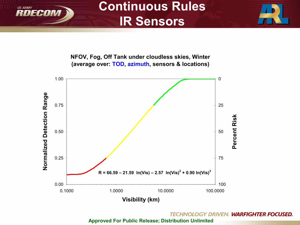
weather conditions, sensors, etc., that were averaged over. Figure 2 shows the four point composite curve “b” (from figure 1) in more detail. In addition, figure 2 also shows the associated composite parametric curve with the T-IWEDA red/yellow/green regions, at the “standard” boundaries of 75% and 25% (since the parametric curves are third order polynomials, it was graphed with more points than the four point dotted curve and, therefore, apparently deviates from the dotted curve). As a consequence of parameterization and normalization, not only is there a continuum of values, but the percent risk associated with these curves can immediately be determined. In figure 2, a secondary axis has been

Figure 2. Composite curve (b in figure 1) averaged over NFOV IR sensors, locations, azimuths, and TOD (see table 1). Note: The scenario parameters are a tank in the inactive state, under cloudless skies, with ground fog.

NFOV, Fog, Off Tank under cloudless skies, Winter (average over: TOD, azimuth, sensors & locations)

0.00

0.25

0.50

0.75

1.00

0.1 1 10 100

Visibility (km)

Nor

mal

ized

Det

ectio

n R

ange

0

25

50

75

100

Perc

ent R

isk

b

TanOffWinCleFog

Figure 1. Normalized Detection Range as a function of target state and orientation, averaged over NFOV IR sensors, and locations (see table 1). Note: The scenario parameters are a tank in the inactive state, under cloudless skies, with ground fog in the morning at 0900 and afternoon at 1500. Also shown are composite curves independent of azimuth (a) and azimuth and TOD (b).

5

added on the right hand side for the percent risk which, for the sensor curves, is nothing more than one minus the normalized detection range. This can be done for any of the combinations for which TAWS runs have been made or, if the particular combination desired is not available, TAWS can be run for those conditions. The coefficients for the parameterized curves for 116 possible combinations may be found in (5). The particular curve in figure 2 can be represented by the third order polynomial

Ndr = 0.3441 + 0.2159 ln(Vis) + 0.0257 ln(Vis)2 – 0.0090 ln(Vis)3 (2)

or, in terms of percent risk

R = (1.0 – Ndr) 100 = 66.59 – 21.59 ln(Vis) – 2.57 ln(Vis)2 + 0.90 ln(Vis)3, (3)

where R is the percent risk.

2.2 Personnel

Where data exists parameterization can be carried out for other, non-sensor, areas. The effect of temperature on Army personnel manual and equipment tasks may be examined using data found in (6). Figure 3 graphically presents that information where it is noted that there is a range of values suitable for parameterization. For the equipment tasks (dashed lines) the upper and lower curves for equipment and manual tasks can be represented, respectively, as

Eff up-equip = 90.101 + 0.5144 T - 0.0151 T2 + 0.0003 T3, (4)

Eff lwr-equip = 81.971 + 0.9167 T – 0.0202 T2 + 0.0002 T3, (5)

Eff up-manual = 76.345 + 1.0777 T – 0.0192 T2 + 0.0001 T3, (6)

Eff lwr-manual = 49.315 + 1.3158 T + 0.0014 T2 – 0.0002 T3, (7)

where Eff is the percent efficiency (subscripts up/lwr (upper/lower) refer to the respective equipment or manual curves), and T is the temperature in °F.


Since T-IWEDA is a qualitative TDA, it is desirable to express equations 4 through 7 as a percent risk, and to also have only

one curve for each of the two types of tasks. This is easily accomplished and the equations representing the equipment and manual tasks are

RE = ½ (Eff up-equip + Eff lwr-equip)

= 86.036 + 0.7156 T - 0.0177 T2 + 0.00025 T3 (8) and

RM = ½ (Eff up-manual + Eff lwr-manual)

= 62.83 + 1.1968 T - 0.0089 T2 - 0.00005 T3 (9)

Figure 3. Effect of temperature on manual and equipment tasks on personnel (7).

Figure 3. Effect of temperature on manual and equipment tasks on personnel (from (6)).

6

where RE is the percent risk for equipment tasks and RM is the percent risk for manual tasks (see right-hand scale, figure 3). These equations must be broken into T-IWEDA regions of applicability. In this case the red/yellow boundary is about -15 °F and the yellow/green boundary is about 20 °F.

2.3 Aircraft

The National Aviation Safety Data Analysis Center (NASDAC) analysis staff performed a study of the National Transportation Safety Board (NTSB) accident and incident database to identify aviation accidents where weather was a causal or contributing factor to an accident. Figures 4 and 5 present a graphical representation of that data for Federal Aviation Administration (FAA) Parts 91 (8) and 135 (9), respectively. Federal Aviation Regulations, or FARs, are rules prescribed by the FAA governing all aviation activities in the United States.

2.3.1 Helicopters

FAA Part 91 and on-demand Part 135 include helicopters. For helicopters we consider Navy data from Cantu (10), and NTSB data for Part 91 and on-demand Part 135. Data from figures 4 and 5, from NTSB’s 2003 accident reports for Parts 91 and 135, and from Cantu’s study on Navy weather related aviation accidents is presented in table 3 (8 – 12). We note than since only 2% of Part 135 is scheduled, we assume that figure 5 values apply directly to on-demand Part 135.

Figure 4. FAA Part 91 NTSB weather related accidents by weather condition (8).


7

Table 3. Data used in determination of helicopter accidents that involve weather.

Source Quantity Part 91 On-demand

Part 135 Navy

No. aircraft accidents 1758 74 395 No. helicopter* accidents 197 27 104 % helicopter accidents 11 36.5 26 No. environmental accidents** 754 - -

No. environmental accidents due to weather**

357 - -

Percent environment accidents due to weather 47 - -

Percent helicopter accidents w/in environment

36 - -

Percent weather related accidents for fleet (all aircraft)

21 30.9 12

% of all weather related helicopter accidents

16.9 27.3 18

% of weather related helicopter accidents 1.9 9.9 5

* rotorcraft (helicopters; gyroplanes and gyrodynes – rotor provides lift only). ** environment is comprised of: weather, terrain, object, light condition, airport.

The last two rows in table 3 are the quantities that are desired: percent of all weather related helicopter accidents, i.e., the number weather related helicopter accidents/total number of helicopter accidents, and percent of weather related helicopter accidents, i.e., the number of helicopters in weather related accidents/total number of aircraft accidents. The former would be of use to wargames and commanders who have access to current weather and want to know the risk of launching a helicopter under those current weather conditions. The latter would be of use to mission planners using long-range forecasts. However, which of these table 3 values to use, Part 91, on-demand Part 135, or Navy, is problematic.

Since the Navy data was taken from a military environment and that data falls between the Part 91 and Part 135 data, we shall use the Navy data, presented in bold in table 3, in the development of risk values for T-IWEDA. Thus, for mission planning purposes, we define the percent of weather related helicopter accidents, as Aw-mp. From table 3 this value, 5%, is thus the percent of helicopters involved in weather accidents compared to all aircraft accidents. For command purposes, we define Aw-cmd as the percent of all weather related helicopter accidents, that is, the number of helicopters involved in weather-related accidents compared to the total number of helicopter accidents. Again from table 3, this value is 18%.

Since helicopters are more often subject to weather accidents than fixed-wing aircraft (10), these values are most likely conservative numbers. Finally, it should be noted that Cantu presents compelling information that, if human factors are included, weather related accident rates are considerably higher.

8

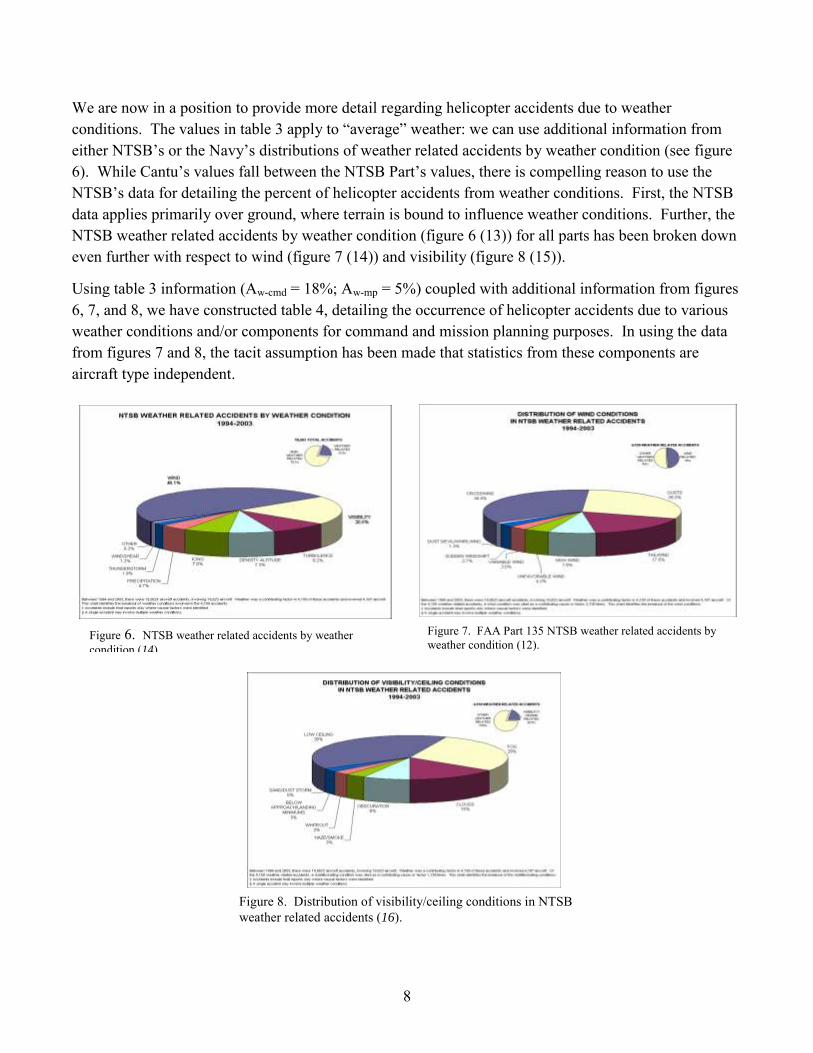
We are now in a position to provide more detail regarding helicopter accidents due to weather conditions. The values in table 3 apply to “average” weather: we can use additional information from either NTSB’s or the Navy’s distributions of weather related accidents by weather condition (see figure 6). While Cantu’s values fall between the NTSB Part’s values, there is compelling reason to use the NTSB’s data for detailing the percent of helicopter accidents from weather conditions. First, the NTSB data applies primarily over ground, where terrain is bound to influence weather conditions. Further, the NTSB weather related accidents by weather condition (figure 6 (13)) for all parts has been broken down even further with respect to wind (figure 7 (14)) and visibility (figure 8 (15)).

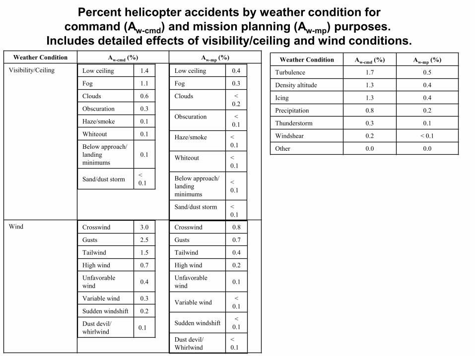
Using table 3 information (Aw-cmd = 18%; Aw-mp = 5%) coupled with additional information from figures 6, 7, and 8, we have constructed table 4, detailing the occurrence of helicopter accidents due to various weather conditions and/or components for command and mission planning purposes. In using the data from figures 7 and 8, the tacit assumption has been made that statistics from these components are aircraft type independent.

Figure 6. NTSB weather related accidents by weather condition (14)


Figure 8. Distribution of visibility/ceiling conditions in NTSB weather related accidents (16).

9

Table 4. Percent helicopter accidents by weather condition for command (Aw-cmd) and mission planning (Aw-mp) purposes, including detailed effects of visibility/ceiling and wind conditions.

Weather Condition Aw-cmd (%) Aw-mp (%)

Visibility/Ceiling 3.7 Low ceiling 1.4 Fog 1.1 Clouds 0.6 Obscuration 0.3 Haze/smoke 0.1 Whiteout 0.1 Below approach/ landing minimums 0.1

Sand/dust storm < 0.1

1.0 Low ceiling 0.4 Fog 0.3 Clouds < 0.2 Obscuration < 0.1 Haze/smoke < 0.1 Whiteout < 0.1 Below approach/ landing minimums < 0.1


Wind 8.6 Crosswind 3.0 Gusts 2.5 Tailwind 1.5 High wind 0.7 Unfavorable wind 0.4 Variable wind 0.3 Sudden windshift 0.2 Dust devil/ whirlwind 0.1

2.4 Crosswind 0.8 Gusts 0.7 Tailwind 0.4 High wind 0.2 Unfavorable wind 0.1 Variable wind < 0.1 Sudden windshift < 0.1 Dust devil/ Whirlwind < 0.1

Turbulence 1.7 0.5

Density altitude 1.3 0.4

Icing 1.3 0.4

Precipitation 0.8 0.2

Thunderstorm 0.3 0.1

Windshear 0.2 < 0.1

Other 0.0 0.0


To make use of the information in table 4, we must consider the red/yellow/green boundaries in T-IWEDA. For rotary-wing aircraft, general operations, a surface wind speed value for the red/yellow boundary is 30 kts and for the yellow/green boundary is 20 kts (16). We now have two points which can be used in the construction of piecewise linear curves: at zero wind speed there will be zero accidents due to wind, and at some wind speed above 30 kts (the red/yellow boundary value), there will be 100% accidents due to wind. The third point will be taken from table 4 – either an 8.6% or 2.4% accident rate due to winds. However, since the accident rates in table 4 represent weather-related accidents for all helicopters under varied wind conditions, the abscissa point (8.6% or 2.4%) for the accident rate probably should not be anchored at the red/yellow boundary. Instead, we will anchor it at halfway between the red/yellow and yellow/green boundaries, or in this instance, at 25 kts. This practice will be

10

followed for all accident rates. Finally, an upper wind speed value must be chosen, a point where one would expect there to be a 100% chance of an accident occurring. This upper value has been chosen here as 50 kts. Therefore for command, the piecewise linear equations will be

Aw-cmd = Rw-cmd

25

0 = 0.344 Ws, (10)

and

Aw-cmd = Rw-cmd

50

25 = 3.656 Ws – 82.8, (11)

where Ws is the wind speed in knots and Rw-cmd

25

0and

Rw-cmd

50

25are the percent risk for wind-related helicopter

accidents for command purposes – the abscissa limits on Rw-cmd are the beginning point (0), the accident rate point (25), and the upper value point (50). The analogous equations for mission planning purposes are

Aw-mp = Rw-mp

25

0 = 0.096 Ws, (12)

and

Aw-mp = Rw-mp

50

25 = 3.904 Ws – 95.2, (13)

where Rw-mp

25

0and Rw-mp

50

25are the percent risk for wind-related helicopter accidents for mission

planning purposes and Ws is as defined above. Equations 10 through 13 are presented graphically in figure 9.

The general category visibility/ceiling can be broken down using the NTSB and Cantu data. Thus we will assume that ceiling alone contributes 1.4/0.4% of helicopter accidents, and low visibility conditions contribute the rest, or 2.3/0.6% for command/mission respectively. Using the methodology above, table 5 presents equations for those weather conditions where suitable T-IWEDA boundary values (17, 18) exist. To anchor the 0% and 100% accident rates, a suitable value for the minimum and maximum boundary values were chosen. Where maximum ceiling heights were unknown, an upper limit of 100 hft was chosen.

0 10 20 30 40 50

Wind Speed (Kts)

0

20

40

60

80

100

Perc

ent R

isk

CommandMission Planning

Figure 9. Piecewise linear curves for weather- related helicopter risk for command and mission planning purposes.

11

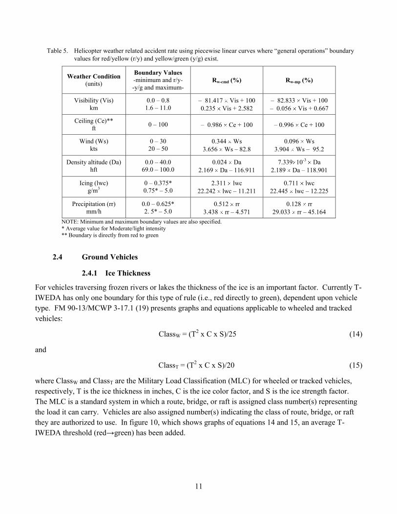
Table 5. Helicopter weather related accident rate using piecewise linear curves where “general operations” boundary values for red/yellow (r/y) and yellow/green (y/g) exist.

Weather Condition (units)

Boundary Values -minimum and r/y- -y/g and maximum-

Rw-cmd (%) Rw-mp (%)

Visibility (Vis) km

0.0 – 0.8 1.6 – 11.0

– 81.417 Vis + 100 0.235 Vis + 2.582

– 82.833 Vis + 100 – 0.056 Vis + 0.667

Ceiling (Ce)** ft 0 – 100 – 0.986 Ce + 100 – 0.996 Ce + 100

Wind (Ws) kts

0 – 30 20 – 50

0.344 Ws 3.656 Ws – 82.8

0.096 Ws 3.904 Ws – 95.2

Density altitude (Da) hft

0.0 – 40.0 69.0 – 100.0

0.024 Da 2.169 Da – 116.911

7.339 10-3 Da 2.189 Da – 118.901

Icing (lwc) g/m3

0 – 0.375* 0.75* – 5.0

2.311 lwc 22.242 lwc – 11.211

0.711 lwc 22.445 lwc – 12.225

Precipitation (rr) mm/h

0.0 – 0.625* 2. 5* – 5.0

0.512 rr 3.438 rr – 4.571

0.128 rr 29.033 rr – 45.164

NOTE: Minimum and maximum boundary values are also specified. * Average value for Moderate/light intensity ** Boundary is directly from red to green

2.4 Ground Vehicles

2.4.1 Ice Thickness

For vehicles traversing frozen rivers or lakes the thickness of the ice is an important factor. Currently T-IWEDA has only one boundary for this type of rule (i.e., red directly to green), dependent upon vehicle type. FM 90-13/MCWP 3-17.1 (19) presents graphs and equations applicable to wheeled and tracked vehicles:

ClassW = (T2 x C x S)/25 (14)

and

ClassT = (T2 x C x S)/20 (15)

where ClassW and ClassT are the Military Load Classification (MLC) for wheeled or tracked vehicles, respectively, T is the ice thickness in inches, C is the ice color factor, and S is the ice strength factor. The MLC is a standard system in which a route, bridge, or raft is assigned class number(s) representing the load it can carry. Vehicles are also assigned number(s) indicating the class of route, bridge, or raft they are authorized to use. In figure 10, which shows graphs of equations 14 and 15, an average T-IWEDA threshold (red→green) has been added.

12

0

10

20

30

40

50

60

0 10 20 30 40 50 60 70

Ice Thickness (inches)

Vehi

cle

Cla

ss

C x S = 1.0

C x S = 0.8

C x S = 0.6

C x S = 0.4

C x S = 1.0

C x S = 0.6

C x S = 0.4

Figure 10. Ice thickness vs. vehicle class with representative T-IWEDA boundaries. The solid lines are wheeled; the dotted lines are tracked.

Here there is only one boundary going from red directly to green. The crosshatched area represents the different boundaries for wheeled (red up to ~15 in.) and tracked (red up to ~20 in.) vehicles. In order to use this graph, the MLC system, which is vehicle specific, needs to be coupled with T-IWEDA’s vehicle types. Unfortunately T-IWEDA does not link vehicle type with MLC. Until that occurs, U.S. Army Engineer School values (20) need to be manually cross referenced with individual vehicle rules.


Assuming that the MLC values have been added to the CRDB, the application of equations (14) and (15) to T-IWEDA are straightforward. These equations would have two regions of applicability, 0 – 15 and 15 – 60 for wheeled vehicles and 0 – 20 and 20 – 60 for tracked vehicles.

3. Conclusions With some judicious choices, many of the T-IWEDA rules can have analytic functions fitted across the step-function boundaries. Since T-IWEDA does not contain quantitative information, other TDAs and sources were used to determine the analytic functions. In particular, information on IR sensors was derived from running TAWS under selected weather conditions. This information was then averaged, curve fit to a third order polynomial as a function of visibility, and concatenated into a data base. Curves, for personnel working in cold regions, were fit and expressed as a function of either manual work or working with equipment. Weather effects on helicopters were also examined. Here NTSB and Navy data were used to determine statistics on weather-related accidents for helicopters. Using that information coupled with boundary limits from the T-IWEDA rule set, piecewise linear curves were fit for a number of weather conditions that contribute to these type of accidents. Finally, the military load factor for vehicles crossing bridges was examined. It was determined that the T-IWEDA rules currently do not contain enough information for this feature to be implemented.

13

References 1. Shirkey, R.C.; Gouveia, M. Weather Impact Decision Aids: Software to Help Plan for Optimal

Sensor and System Performance, Crosstalk, the Journal of Defense Software Engineering 2002, 15, (12), 17–21.

2. ACQUIRE 1995. ACQUIRE Range Performance Model for Target Acquisition Systems 1995, Version 1 User’s Guide, U.S. Army CECOM Night Vision and Electronic Sensors Directorate Report.

3. Shirkey, R.C.; Tofsted, D. High Resolution Electro-Optical Aerosol Phase Function Database PFNDAT 2006, ARL-TR-3877, U.S. Army Research Laboratory: White Sands Missile Range, NM, 2006 (ADA458924).

4. Press, W. H.; Teukolsky, S. A.; Vetterling, W. T.; Flannery, B. P. Numerical Recipes in Fortran 77: The Art of Scientific Computing, 2nd ed ., Cambridge University Press: New York, NY, 2003.

5. Shirkey, R.C., Determination of Risk Levels for Rule-Based Weather Decision Aids, Army Research Laboratory Technical Report ARL-TR-4586, September 20008.

6. Richmond, P., Ed. Notes for Cold Weather Military Operations, Cold Regions Research and Engineering Laboratory Special Report 91–30, December 1991.

7. Abele, G., Effect of Cold Weather on Productivity, in Technology Transfer Opportunities for the Construction Engineering Commmunity, Cold Regions Research and Engineering Laboratory Miscellaneous Publication MP2152, 1986. http://www.crrel.usace.army.mil/library/frequentlyrequested.html

8. http://www.asias.faa.gov/aviation_studies/weather_study/part91.html

9. http://www.asias.faa.gov/aviation_studies/weather_study/part135.html

10. Cantu, Ruben A. The Role Of Weather In Class A Naval Aviation Mishaps FY90–98, Master’s Thesis, Naval Postgraduate School, Monterey, CA, March 2001.

11. Annual Review of Aircraft Accident Data, U.S. General Aviation, Calendar Year 2003, National Transportation Safety Board/ARG-07/01, PB2007-105388, November 29, 2006.

12. Annual Review of Aircraft Accident Data, U. S. Air Carrier Operations Calendar Year 2003, National Transportation Safety Board/ARC-07/01, PB2007-105389, December 2006.

13. http://www.asias.faa.gov/aviation_studies/weather_study/categories.html

14. http://www.asias.faa.gov/aviation_studies/weather_study/windcond.html

15. http://www.asias.faa.gov/aviation_studies/weather_study/viscecon.html

http://www.crrel.usace.army.mil/library/frequentlyrequested.html

http://www.asias.faa.gov/aviation_studies/weather_study/part91.html

http://www.asias.faa.gov/aviation_studies/weather_study/part135.html

http://www.asias.faa.gov/aviation_studies/weather_study/categories.html

http://www.asias.faa.gov/aviation_studies/weather_study/windcond.html

http://www.asias.faa.gov/aviation_studies/weather_study/viscecon.html

14

16. Intelligence Preparation of the Battlefield, FM 34-130, p. B-21, Dept. of Army, Washington D.C., July 1994.

17. The Centralized Rules Data Base, https://www.us.army.mil/suite/page/494483

18. Operator’s Manual for UH-60A Helicopters, Uh-60L Helicopters and EH-60A Helicopters, TM 1-1520-237-10, p. 5-23, Dept. of Army, Washington D.C., April 2000.

19. River-Crossing Operations, FM 90-13/MCWP 3-17.1, Dept. of Army, Washington D.C., January 1998.

20. http://www.wood.army.mil/cellx/information%20folders/mil%20load%20class/ mlc%20web%20document.html

https://www.us.army.mil/suite/page/494483*

http://www.wood.army.mil/cellx/information%20folders/mil%20load%20class/%0bmlc%20web%20document.html

http://www.wood.army.mil/cellx/information%20folders/mil%20load%20class/%0bmlc%20web%20document.html

Approved For Public Release; Distribution Unlimited

Risk Levels for Rule-BasedWeather Decision Aids

Dr Richard ShirkeyArmy Research Laboratory

Battlefield Environment Division WSMR NM

Ph: (575) [email protected]

ITEA LVC 12-15 Jan 2009



Rules, What are They?

A rule is simply a critical value associated with aspecific system

e.g. Surface winds greater than 30 knots preclude helicopter takeoff or landing

Using critical values these rules are coded into severe, moderate, or no impact. The rule above would be red. An example of a yellow rule for the same system would be

Surface windspeed greater than 27 knots may impact aircraft hover


Rules, How are limits determined?

Impact CriteriaGreen

(favorable) Degradation < ~25%

Amber (marginal) Degradation = ~25 to ~75 %

Red (unfavorable) Degradation > ~75%

Army FM 34-81-1, Battlefield Weather Effects, defines severe as reducing normal effectiveness greater than 75%, moderate as reducing normal effectiveness from 25 – 75%, and no impact as a reduction in normal effectiveness less than 25%


Rules, Where do they come from?

Rules are collected from service specific field manuals, training

centers and schools.


Rules Database

The Weather Impacts Database will contains more than 11000 weather impact rules and critical value thresholds for severe (“red”) and moderate (“amber”) impacts

They fall into these 12 critical value parameter

categories

(Visibility includes low clouds, fog and reduced visual/IR sensor ranges)


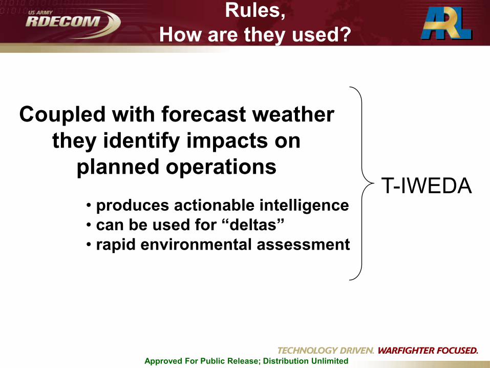
Rules,How are they used?

Coupled with forecast weather they identify impacts on

planned operations• produces actionable intelligence• can be used for “deltas”• rapid environmental assessment

T-IWEDA


T-IWEDA stands for the Tri-Service IntegratedWeather Effects Decision Aid

It is a collection of system rules with associatedcritical values for aiding the commander select

an appropriate platform, system or sensor under given weather conditions

Results are displayed via a red/amber/green colormatrix overlaid on a background map

What is T-IWEDA?


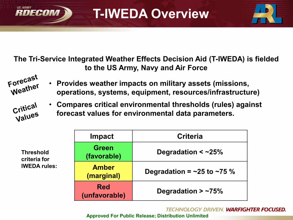
• Provides weather impacts on military assets (missions, operations, systems, equipment, resources/infrastructure)

• Compares critical environmental thresholds (rules) against forecast values for environmental data parameters.

The Tri-Service Integrated Weather Effects Decision Aid (T-IWEDA) is fielded to the US Army, Navy and Air Force

Threshold criteria for IWEDA rules:

Impact CriteriaGreen

(favorable) Degradation < ~25%

Amber (marginal) Degradation = ~25 to ~75 %

Red (unfavorable) Degradation > ~75%

T-IWEDA Overview


T-IWEDA


RULES: HOW RED IS RED?

• T-IWEDA rules are implemented in terms of step function stop light charts

• Red-Yellow-Green • Boundaries are 75% (R/Y) and 25% (Y/G)

reduction in effectiveness

• Reality dictates boundaries should be fuzzy

• An extremely useful piece of information would be knowing how quickly, or at what rate, transitions occur between and within the red/yellow/green boundaries/cells


Step Function vs.Continuous Curve

Visibility (km)

Nor

mal

ized

D

etec

tion

Ran

ge

0

0.5

1

0.1 1 10 100


Visibility (km)

Nor

mal

ized

D

etec

tion

Ran

ge Rural, ClearFog, Clear

0

0.5

1

0.1 1 10 100

Step Function vs.Continuous Curve


Continuous Rules

• To mitigate the step function problem, a series of weather specific curves that transition from red to yellow to green in a continuous manner have been developed using measured and modeled resources for

• IR Sensors• Helicopters• Cold weather personnel

equipment and manual tasks


IR Sensors

Continuous Rules


Continuous RulesIR Sensors

• The Target Acquisition Weapons Software (TAWS) was run for select weather & target geometries.

26 IR Sensors FOV platform LOS azimuth

narrow and wide helicopter at 300’ altitude N, S, E, W

Targets platform state Orientation

T80 and armored personnel carrier (APC) inactive and exercised north facing

Meteorology visibility aerosols cloud cover

0.1, 1.0, 10, 100 km rural (50% relative humidity),

fog (moderate radiation) cloudless, overcast

Locale longitude latitude Background

0 0 , 30 N desert sand

Season 0 (equator) 30 N

equinox and winter solstice summer and winter solstices

TOD 0900 and 1500

TAWS provides acquisition ranges as a function of weather, target type and time of day


NFOV, Fog, Off Tank under cloudless skies, Winter f(TOD & Azimuth)

(average over: sensors & locations)

0

0.25

0.5

0.75

1

0.1 1 10 100

Visibility (km)

Nor

mal

ized

Det

ectio

n R

ange

TanOff900WinNorCleFog

TanOff900WinSouCleFog

TanOff900WinEasCleFog

TanOff900WinWesCleFog







NFOV, Fog, Off Tank under cloudless skies, Winter f(TOD & Azimuth)

(average over: sensors & locations)

0

0.25

0.5

0.75

1

0.1 1 10 100

Visibility (km)

Nor

mal

ized

Det

ectio

n R

ange









TanOff900WinCleFog

TanOffWinCleFog

azimuth

TOD



NFOV, Fog, Off Tank under cloudless skies, Winter (average over: TOD, azimuth, sensors & locations)

0.00

0.25

0.50

0.75

1.00

0.1000 1.0000 10.0000 100.0000

Visibility (km)

Nor

mal

ized

Det

ectio

n R

ange

0

25

50

75

100

Perc

ent R

isk

R = 66.59 – 21.59 ln(Vis) – 2.57 ln(Vis)2 + 0.90 ln(Vis)3



Helicopters

Continuous Rules


Helicopter Accidents Related to WeatherNational Transportation Safety Board (NTSD)

Continuous RulesHelicopters



Naval helicopter accident data obtained fromMaster’s thesis


SourceQuantity Part 91 On-demand

Part 135 Navy

No. aircraft accidents 1758 74 395

No. helicopter accidents197 27 104

% helicopter accidents 11 36.5 26

No. environmental accidents 754 - -

No. environmental accidents due to weather** 357 - -

Percent environment accidents due to weather 47 - -

Percent helicopter accidents w/in environment 36 - -

Percent weather related accidents for fleet(all aircraft)

21 30.9 12

% of all weather related helicopter accidents 16.9 27.3 18

% of weather related helicopter accidents 1.9 9.9 5

Concatenation of NTSB and Navy data

Wargamers & commanders who have access to current weather conditions

Mission planners using long-range forecasts.



Visibility/Ceiling

Wind

Low ceiling 1.4

Fog 1.1

Clouds 0.6

Obscuration 0.3

Haze/smoke 0.1

Whiteout 0.1

Below approach/ landing minimums

0.1


Low ceiling 0.4

Fog 0.3

Clouds < 0.2

Obscuration < 0.1

Haze/smoke < 0.1

Whiteout < 0.1

Below approach/ landing minimums

< 0.1


Crosswind 3.0

Gusts 2.5

Tailwind 1.5

High wind 0.7

Unfavorable wind 0.4

Variable wind 0.3

Sudden windshift 0.2

Dust devil/ whirlwind 0.1

Crosswind 0.8

Gusts 0.7

Tailwind 0.4

High wind 0.2

Unfavorable wind 0.1

Variable wind < 0.1

Sudden windshift < 0.1

Dust devil/ Whirlwind

< 0.1


Turbulence 1.7 0.5

Density altitude 1.3 0.4

Icing 1.3 0.4

Precipitation 0.8 0.2

Thunderstorm 0.3 0.1

Windshear 0.2 < 0.1

Other 0.0 0.0

Percent helicopter accidents by weather condition forcommand (Aw-cmd) and mission planning (Aw-mp) purposes.

Includes detailed effects of visibility/ceiling and wind conditions.


0 10 20 30 40 50

Wind Speed (Kts)

0

20

40

60

80

100

Perc

ent R

isk

CommandMission Planning

Piecewise linear curves for weather-related helicopter riskfor command and mission planning purposes



Continuous Rules

Cold weather personnel equipment and manual tasks

Effect of temperature on Army personnel

manual and equipment tasks*

Continuous RulesPersonnel

* Notes for Cold Weather Military Operations, P.W. Richmond (Ed), CRREL-SR-91-30, 1991.

Effupr-equip = 90.101 + 0.5144 T 0.0151 T2 + 0.0003 T3

Efflwr-equip = 81.971 + 0.9167 T 0.0202 T2 + 0.0002 T3

Effupr-man = 76.345 + 1.0777 T 0.0192 T2 + 0.0001 T3

Efflwr-man = 49.315 + 1.3158 T + 0.0014 T2 0.0002 T3 Dashed: Equipment TasksSolid: Manual Tasks

Temperature (ºF)

-60 -40 -20 0 20 40

Effi

cien

cy (%

)

0

20

40

60

80

100


Continuous RulesPersonnel

RE = 86.036 + 0.7156 T - 0.0177 T2 + 0.00025 T3

RM = 62.83 + 1.1968 T - 0.0089 T2 - 0.00005 T3

Boundaries determined by 25%/75%

criteria

0

20

40

60

80

100

-60 -40 -20 0 20 40

Temperature (deg F)

Effic

ienc

y (%

)

0

20

40

60

80

100

Risk

(%)

(

(


Point of Contact:

Dr. Richard ShirkeyLead DoD Tri-Service IWEDA Consortium(575) 678-5470; [email protected]

US Army Research Laboratory CISD/Battlefield Environment DivisionAMSRD-ARL-CI-EMWhite Sands Missile Range, NM 88002-5501

?


risk levels for rule-based weather decision · pdf filerisk levels for rule-based weather...

Documents