Right Hand Side Right Hand Side (Independent) Variables(Independent) Variables

Ciaran S. PhibbsCiaran S. Phibbs

Independent VariablesIndependent Variables

Regression models make several Regression models make several assumptions about the independent assumptions about the independent variablesvariables

The purpose of this talk is to examine The purpose of this talk is to examine some of the more common problems, some of the more common problems, and some methods of fixing themand some methods of fixing them

Focus on things not likely to be covered Focus on things not likely to be covered in standard econometric classesin standard econometric classes

OutlineOutline

HeteroskedasticityHeteroskedasticity Clustering of observationsClustering of observations Functional formFunctional form Testing for multicollinearityTesting for multicollinearity

HeteroskedasticityHeteroskedasticity

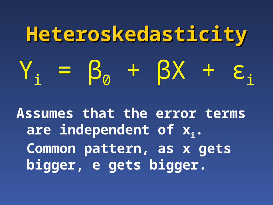
Yi = β0 + βX + εi

Assumes that the error terms are independent of xi. Common pattern, as x gets bigger, e gets bigger.

HeteroskedasticityHeteroskedasticity

• Biased standard errors• Parameter estimates unbiased, but

inefficient

• Simple solution, robust option in Stata uses Huber-White method to correct standard errors.

ClusteringClustering

Yi = β0 + βX + εi

Assumes that the error terms are uncorrelated

Clustering is a common problem, for example, patients are clustered within hospitals

ClusteringClustering

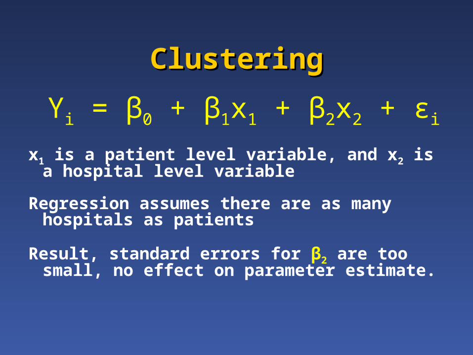
Yi = β0 + β1x1 + β2x2 + εi

x1 is a patient level variable, and x2 is a hospital level variable

Regression assumes there are as many hospitals as patients

Result, standard errors for β2 are too small, no effect on parameter estimate.

Correcting for ClusteringCorrecting for Clustering

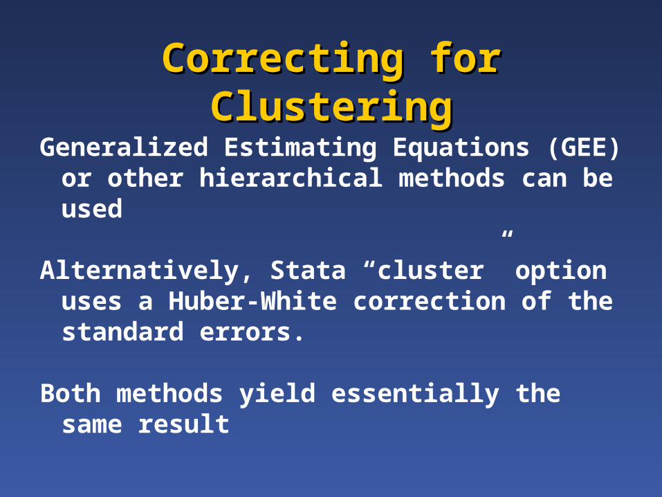
Generalized Estimating Equations (GEE) or other hierarchical methods can be used

Alternatively, Stata “cluster” option uses a Huber-White correction of the standard errors.

Both methods yield essentially the same result

Example of ClusteringExample of Clustering

I have a research project that is looking at the effects of NICU patient volume and NICU level on mortality. NEJM 2007.

I apologize for not having a VA example, but I had already addressed the issues to be covered, and could easily do custom runs for this talk.

ClusteringClustering

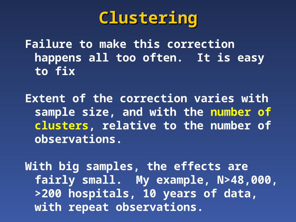
Failure to make this correction happens all too often. It is easy to fix

Extent of the correction varies with sample size, and with the number of clusters, relative to the number of observations.

With big samples, the effects are fairly small. My example, N>48,000, >200 hospitals, 10 years of data, with repeat observations.

Example of ClusteringExample of ClusteringLevel of Care/VLBW volumeLevel of Care/VLBW volume OR OR 95% C.I. unadjusted95% C.I. unadjusted

Level 1 ≤10 VLBW infantsLevel 1 ≤10 VLBW infants 2.72**2.72** (2.37, 3.13)(2.37, 3.13) 2.40, 3.072.40, 3.07

Level 2 11-25 VLBW infantsLevel 2 11-25 VLBW infants 1.88**1.88** (1.56, 2.26)(1.56, 2.26) 1.64, 2.151.64, 2.15

Level 2 >25 VLBW infantsLevel 2 >25 VLBW infants 1.221.22 (0.98, 1.52)(0.98, 1.52) 1.09, 1.361.09, 1.36

Level 3B or 3C ≤25 VLBW Level 3B or 3C ≤25 VLBW 1.51**1.51** (1.17, 1.95)(1.17, 1.95) 1.25, 1.781.25, 1.78

Level 3B or 3C 26-50 VLBW Level 3B or 3C 26-50 VLBW 1.30**1.30** (1.12, 1.50)(1.12, 1.50) 1.17, 1.421.17, 1.42

Level 3B, 3C, or 3D 51-100Level 3B, 3C, or 3D 51-100 1.19*1.19* (1.04, 1.37)(1.04, 1.37) 1.10, 1.291.10, 1.29

Functional FormFunctional Form

Yi = β0 + βX + εi

βX assumes that each variable in X has a linear relationship with Y

This is not always the case, can This is not always the case, can result in a mis-specified modelresult in a mis-specified model

You should check for the functional form for every non-binary variable in your model.

There are formal tests for model specification, some of which you may have been exposed to in classes. But, these tests don’t really show you what you are looking at.

Using Dummy Variables to Using Dummy Variables to Examine Functional FormExamine Functional Form

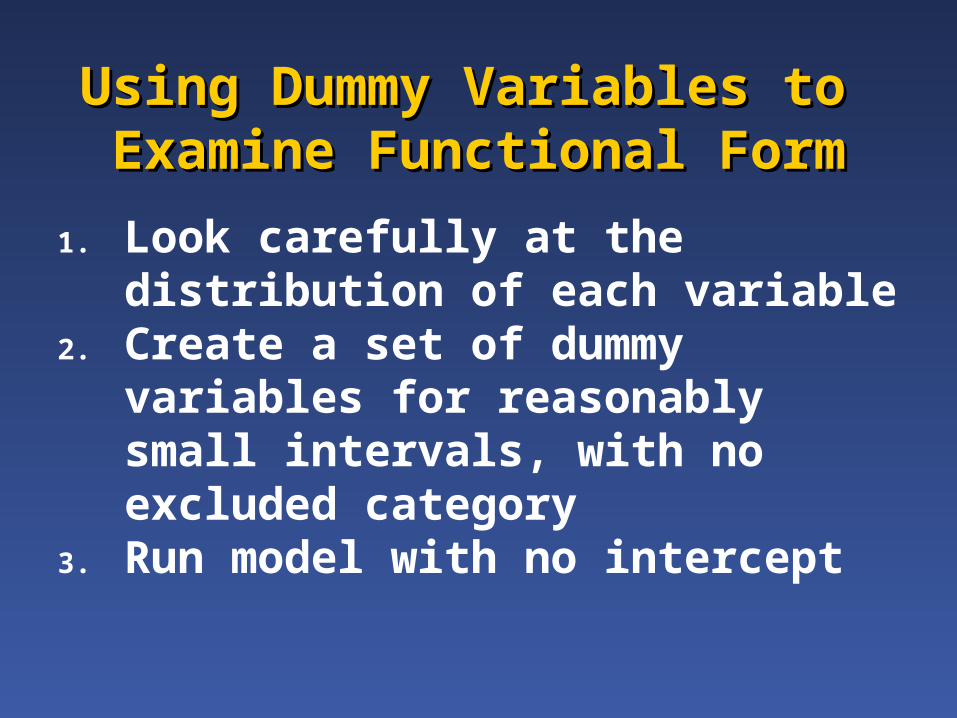
1. Look carefully at the distribution of each variable

2. Create a set of dummy variables for reasonably small intervals, with no excluded category

3. Run model with no intercept

Example of Using Dummy Example of Using Dummy Variables to Examine Functional FormVariables to Examine Functional Form

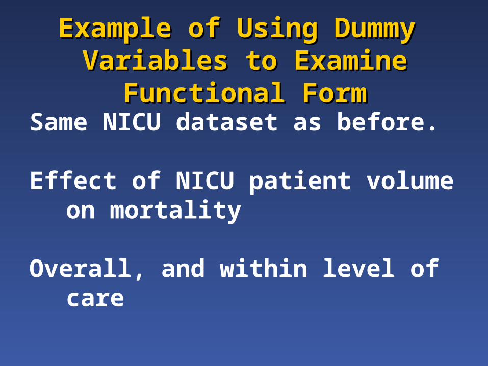
Same NICU dataset as before.

Effect of NICU patient volume on mortality

Overall, and within level of care

Example of Using Dummy Example of Using Dummy Variables to Examine Functional Variables to Examine Functional

FormForm

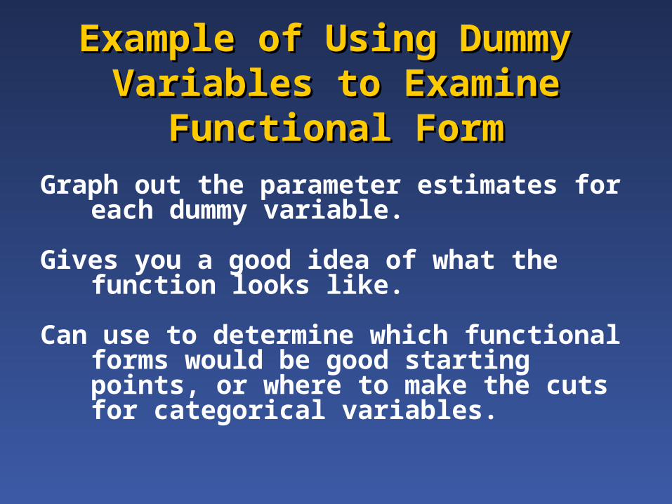
Graph out the parameter estimates for each dummy variable.

Gives you a good idea of what the function looks like.

Can use to determine which functional forms would be good starting points, or where to make the cuts for categorical variables.

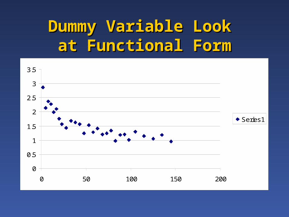
Dummy Variable Look Dummy Variable Look at Functional Format Functional Form

0

0.5

1

1.5

2

2.5

3

3.5

0 50 100 150 200

Series1

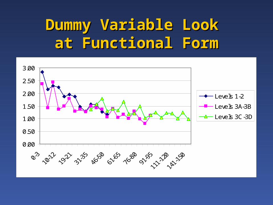
Dummy Variable Look Dummy Variable Look at Functional Format Functional Form

0.00

0.50

1.00

1.50

2.00

2.50

3.00

Levels 1-2

Levels 3A-3B

Levels 3C-3D

Example of Using Dummy Example of Using Dummy Variables to Examine Functional FormVariables to Examine Functional Form

For some applications you may just want to use dummy variables, instead of a continuous functional form. This may be especially useful when there are complex relationships. It can be very difficult to get a continuous function to accurately predict across the entire range of values.

Aside, categorical variables frequently easier to present to medical audiences.

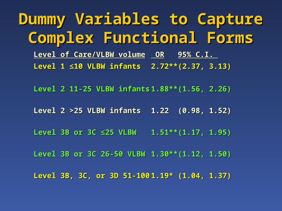
Dummy Variables to Capture Dummy Variables to Capture Complex Functional FormsComplex Functional Forms

Level of Care/VLBW volumeLevel of Care/VLBW volume OR OR 95% C.I. 95% C.I.

Level 1 ≤10 VLBW infantsLevel 1 ≤10 VLBW infants 2.72**2.72** (2.37, 3.13)(2.37, 3.13)

Level 2 11-25 VLBW infantsLevel 2 11-25 VLBW infants 1.88**1.88** (1.56, 2.26)(1.56, 2.26)

Level 2 >25 VLBW infantsLevel 2 >25 VLBW infants 1.221.22 (0.98, 1.52)(0.98, 1.52)

Level 3B or 3C ≤25 VLBW Level 3B or 3C ≤25 VLBW 1.51**1.51** (1.17, 1.95)(1.17, 1.95)

Level 3B or 3C 26-50 VLBW Level 3B or 3C 26-50 VLBW 1.30**1.30** (1.12, 1.50)(1.12, 1.50)

Level 3B, 3C, or 3D 51-100Level 3B, 3C, or 3D 51-100 1.19*1.19* (1.04, 1.37)(1.04, 1.37)

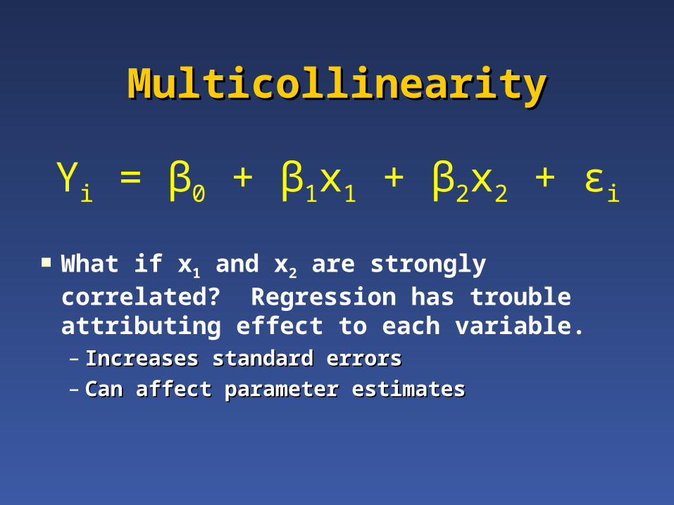
MulticollinearityMulticollinearity

Yi = β0 + β1x1 + β2x2 + εi

What if x1 and x2 are strongly correlated? Regression has trouble attributing effect to each variable. – Increases standard errorsIncreases standard errors– Can affect parameter estimatesCan affect parameter estimates

MulticollinearityMulticollinearity Strong simple correlation, you have a problem. Strong simple correlation, you have a problem.

But, can be hidden problems not detected by But, can be hidden problems not detected by simple correlations.simple correlations.

Variance Inflation Factor (/VIF SAS, vif in Variance Inflation Factor (/VIF SAS, vif in Stata Regression Diagnostics) measures the Stata Regression Diagnostics) measures the inflation in the variances of each parameter inflation in the variances of each parameter estimate due to collinearities among the estimate due to collinearities among the regressorsregressors

Tolerance, which is 1/VIFTolerance, which is 1/VIF VIF > 10 implies significant collinearity VIF > 10 implies significant collinearity

problemproblem

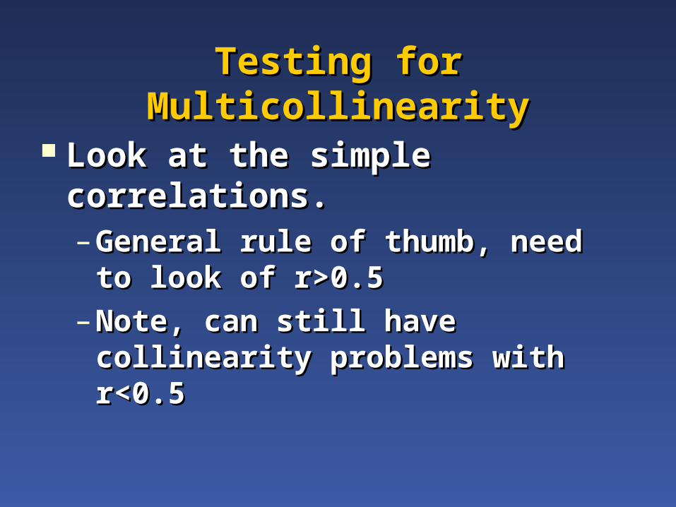
Testing for MulticollinearityTesting for Multicollinearity

Look at the simple correlations. Look at the simple correlations. – General rule of thumb, need to look of General rule of thumb, need to look of

r>0.5r>0.5

– Note, can still have collinearity problems Note, can still have collinearity problems with r<0.5 with r<0.5

Example of Correlation and VIFExample of Correlation and VIF

Study of nurse staffing and patient Study of nurse staffing and patient outcomes. outcomes. – Problem variables. RN HPBD and (RN Problem variables. RN HPBD and (RN

NPBD)**2NPBD)**2– R=0.92R=0.92– VIF range, 10-40, depending on subsetVIF range, 10-40, depending on subsetResult, many fewer statistically significant Result, many fewer statistically significant

results than we expected. results than we expected.

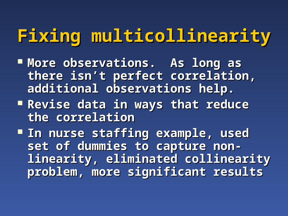
Fixing multicollinearityFixing multicollinearity More observations. As long as there isn’t More observations. As long as there isn’t

perfect correlation, additional observations perfect correlation, additional observations help.help.

Revise data in ways that reduce the Revise data in ways that reduce the correlationcorrelation

In nurse staffing example, used set of In nurse staffing example, used set of dummies to capture non-linearity, dummies to capture non-linearity, eliminated collinearity problem, more eliminated collinearity problem, more significant resultssignificant results

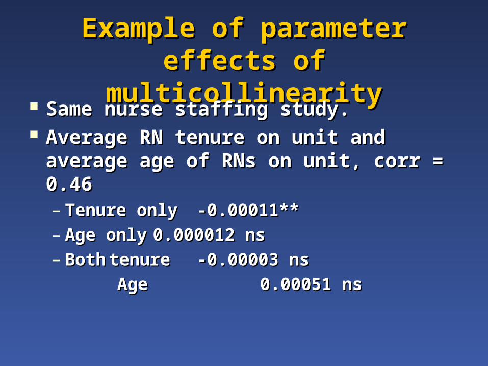
Example of parameter effects of Example of parameter effects of multicollinearitymulticollinearity

Same nurse staffing study.Same nurse staffing study. Average RN tenure on unit and average age Average RN tenure on unit and average age

of RNs on unit, corr = 0.46of RNs on unit, corr = 0.46– Tenure onlyTenure only -0.00011**-0.00011**– Age onlyAge only 0.000012 ns0.000012 ns– BothBoth tenuretenure -0.00003 ns-0.00003 ns

AgeAge 0.00051 ns0.00051 ns

MulticollinearityMulticollinearity Strong simple correlation, you have a Strong simple correlation, you have a

problem. But, can be hidden problems not problem. But, can be hidden problems not detected by simple correlations.detected by simple correlations.

Regression, n-space, correlation on each of Regression, n-space, correlation on each of the regression planes can matter. the regression planes can matter.

Collin option in SAS, looks at how much of Collin option in SAS, looks at how much of the variation in each eigen vector is the variation in each eigen vector is explained by each variable. Intuitively, the explained by each variable. Intuitively, the correlation in the Nth dimension of the correlation in the Nth dimension of the regression.regression.

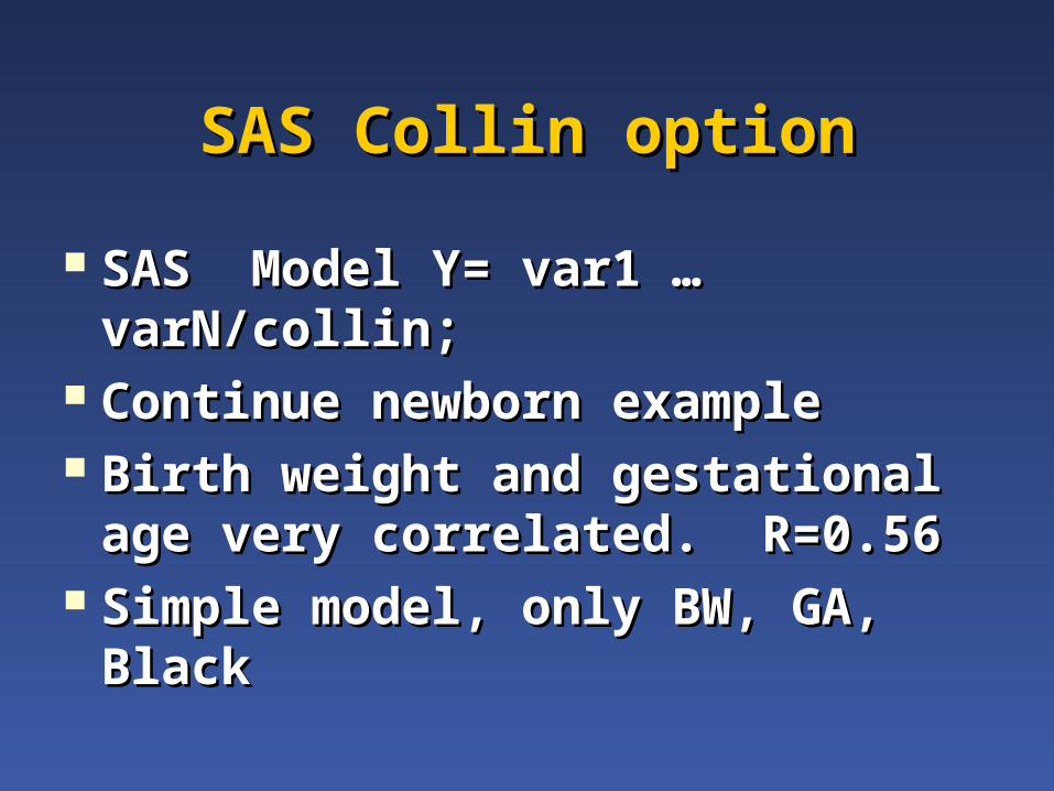
SAS Collin optionSAS Collin option

SAS Model Y= var1 … varN/collin;SAS Model Y= var1 … varN/collin; Continue newborn exampleContinue newborn example Birth weight and gestational age very Birth weight and gestational age very

correlated. R=0.56correlated. R=0.56 Simple model, only BW, GA, BlackSimple model, only BW, GA, Black

Interpreting Collin outputInterpreting Collin output

Condition index >10 indicates a Condition index >10 indicates a collinearity problemcollinearity problem

Condition index >100 indicates an Condition index >100 indicates an extreme problemextreme problem

There is strong correlation in the There is strong correlation in the variance proportion if 2 or more variance proportion if 2 or more variables have values >0.50.variables have values >0.50.

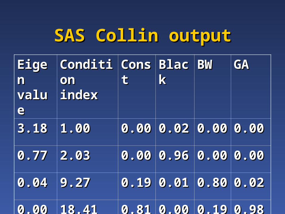
SAS Collin outputSAS Collin output

Eigen Eigen valuevalue

Condition Condition indexindex

ConstConst BlackBlack BWBW GAGA

3.183.18 1.001.00 0.000.00 0.020.02 0.000.00 0.000.00

0.770.77 2.032.03 0.000.00 0.960.96 0.000.00 0.000.00

0.040.04 9.279.27 0.190.19 0.010.01 0.800.80 0.020.02

0.0010.001 18.4118.41 0.810.81 0.000.00 0.190.19 0.980.98

Fixing multicollinearity,Fixing multicollinearity,NICU exampleNICU example

Used dummy variables for BW in 100g Used dummy variables for BW in 100g intervals to 1000g, then 250g intervals.intervals to 1000g, then 250g intervals.

Separate BW dummies for singleton males, Separate BW dummies for singleton males, singleton females, and multiple births,singleton females, and multiple births,

Gestation in 2 week intervals.Gestation in 2 week intervals. Max condition index < 8, i.e. no serious Max condition index < 8, i.e. no serious

collinearity problem. collinearity problem. Model predictions also improved.Model predictions also improved.

Dummy Variables To Fix Dummy Variables To Fix CollinearityCollinearity

0

2

46

8

10

1214

16

18

650 750 850 950 1125 1375

Birth Weight

Odds R

atios

Female

Multiple

Male

References References

Belsley, D.A., Kuh, E., and Welsch, Belsley, D.A., Kuh, E., and Welsch, R.E. (1980) Regression Diagnositics. R.E. (1980) Regression Diagnositics. New York, John Wiley & Sons. New York, John Wiley & Sons.