review of filtering - brown university department of...
TRANSCRIPT


Review of Filtering
• Filtering in frequency domain
– Can be faster than filtering in spatial domain (for large filters)
– Can help understand effect of filter
– Algorithm:
1. Convert image and filter to fft (fft2 in matlab)
2. Pointwise-multiply ffts
3. Convert result to spatial domain with ifft2
Did anyone play with the code?
Hays

Review of Filtering
• Linear filters for basic processing
– Edge filter (high-pass)
– Gaussian filter (low-pass)
FFT of Gaussian
[-1 1]
FFT of Gradient Filter
Gaussian
Hays

More Useful Filters
1st Derivative of Gaussian
(Laplacian of Gaussian)
Earl F. Glynn

Things to Remember
• Sometimes it makes sense to think of images and filtering in the frequency domain– Fourier analysis
• Can be faster to filter using FFT for large images• N logN vs. N2 for auto-correlation
• Images are mostly smooth– Basis for compression
• Remember to low-pass before sampling• Otherwise you create aliasing
Hays

EDGE / BOUNDARY DETECTION
Many slides from James Hays, Lana Lazebnik, Steve Seitz, David Forsyth, David Lowe, Fei-Fei Li, and Derek Hoiem
Szeliski 4.2

Edge detection
• Goal: Identify visual changes (discontinuities) in an image.
• Intuitively, semantic information is encoded in edges.
• What are some ‘causes’ ofvisual edges?
Source: D. Lowe

Origin of Edges
• Edges are caused by a variety of factors
depth discontinuity
surface color discontinuity
illumination discontinuity
surface normal discontinuity
Source: Steve Seitz

Why do we care about edges?
• Extract information
– Recognize objects
• Help recover geometry and viewpoint
Vanishingpoint
Vanishingline
Vanishingpoint
Vertical vanishingpoint
(at infinity)

Closeup of edges
Source: D. Hoiem

Closeup of edges
Source: D. Hoiem

Closeup of edges
Source: D. Hoiem

Closeup of edges
Source: D. Hoiem
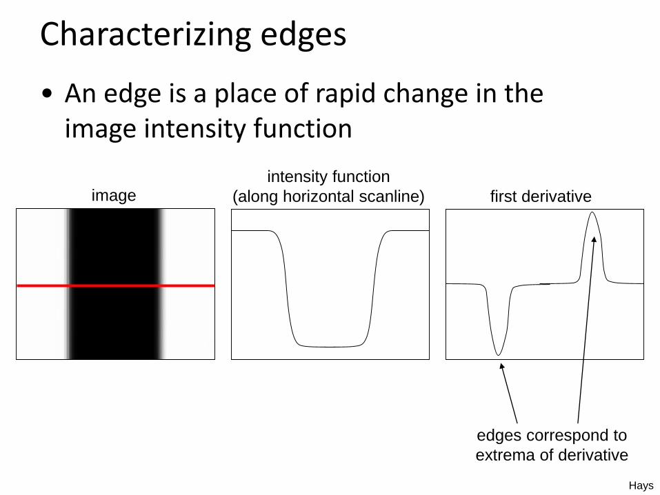
Characterizing edges
• An edge is a place of rapid change in the image intensity function
imageintensity function
(along horizontal scanline) first derivative
edges correspond to
extrema of derivative
Hays

Intensity profile
Source: D. Hoiem

With a little Gaussian noise
Gradient
Source: D. Hoiem

Effects of noise• Consider a single row or column of the image
– Plotting intensity as a function of position gives a signal
Where is the edge?Source: S. Seitz

Effects of noise
• Difference filters respond strongly to noise
– Image noise results in pixels that look very different from their neighbors
– Generally, the larger the noise the stronger the response
• What can we do about it?
Source: D. Forsyth

Solution: smooth first
• To find edges, look for peaks in )( gfdx
d
f
g
f * g
)( gfdx
d
Source: S. Seitz
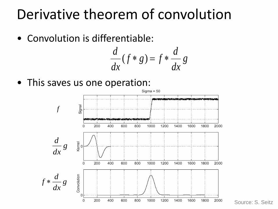
• Convolution is differentiable:
• This saves us one operation:
gdx
dfgf
dx
d )(
Derivative theorem of convolution
gdx
df
f
gdx
d
Source: S. Seitz

Derivative of 2D Gaussian filter
* [1 -1] =
Hays

• Smoothed derivative removes noise, but blurs edge. Also finds edges at different “scales”.
1 pixel 3 pixels 7 pixels
Tradeoff between smoothing and localization
Source: D. Forsyth

Think-Pair-Share
What is a good edge detector?
Do we lose information when we look at edges?
Are edges ‘complete’ as a representation of images?

Designing an edge detector• Criteria for a good edge detector:
– Good detection: the optimal detector should find all real edges, ignoring noise or other artifacts
– Good localization• the edges detected must be as close as possible to
the true edges• the detector must return one point only for each
true edge point
• Cues of edge detection– Differences in color, intensity, or texture across the
boundary– Continuity and closure– High-level knowledge
Source: L. Fei-Fei

Designing an edge detector
• “All real edges”
• We can aim to differentiate later on which edges are ‘useful’ for our applications.
• If we can’t find all things which could be called an edge, we don’t have that choice.
• Is this possible?

Closeup of edges
Source: D. Hoiem

Elder – Are Edges Incomplete? 1999
What information would we need to
‘invert’ the edge detection process?

Elder – Are Edges Incomplete? 1999
Edge ‘code’:
- position,
- gradient magnitude,
- gradient direction,
- blur.

Where do humans see boundaries?
• Berkeley segmentation database:http://www.eecs.berkeley.edu/Research/Projects/CS/vision/grouping/segbench/
image human segmentation gradient magnitude
pB slides: Hays

pB boundary detector
Figure from Fowlkes
Martin, Fowlkes, Malik 2004: Learning to Detect
Natural Boundaries…
http://www.eecs.berkeley.edu/Research/Projects/C
S/vision/grouping/papers/mfm-pami-boundary.pdf

Brightness
Color
Texture
Combined
Human

pB Boundary Detector
Figure from Fowlkes

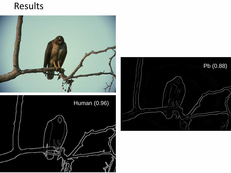
Results
Human (0.95)
Pb (0.88)
Results
Human
Pb
Human (0.96)
Global PbPb (0.88)

Human (0.95)
Pb (0.63)

Human (0.90)
Pb (0.35)
For more:
http://www.eecs.berkeley.edu/Research/Projects
/CS/vision/bsds/bench/html/108082-color.html

45 years of boundary detection
Source: Arbelaez, Maire, Fowlkes, and Malik. TPAMI 2011 (pdf)

State of edge detection
• Local edge detection works well
– ‘False positives’ from illumination and texture edges (depends on our application).
• Some methods to take into account longer contours
• Modern methods that actually “learn” from data.
• Poor use of object and high-level information.
Hays

Summary: Edges primer
• Edge detection to identifyvisual change in image
• Derivative of Gaussian and linear combinationof convolutions
• What is an edge?What is a good edge?
gdx
df
f
gdx
d

Canny edge detector
• Probably the most widely used edge detector in computer vision.
• Theoretical model: step-edges corrupted by additive Gaussian noise.
• Canny showed that first derivative of Gaussian closely approximates the operator that optimizes the product of signal-to-noise ratioand localization.
J. Canny, A Computational Approach To Edge Detection, IEEE
Trans. Pattern Analysis and Machine Intelligence, 8:679-714, 1986.
L. Fei-Fei
22,000 citations!

Demonstrator Image
rgb2gray(‘img.png’)

Canny edge detector
1. Filter image with x, y derivatives of Gaussian
Source: D. Lowe, L. Fei-Fei

Derivative of Gaussian filter
x-direction y-direction

Compute Gradients
X Derivative of Gaussian Y Derivative of Gaussian
(x2 + 0.5 for visualization)

Canny edge detector
1. Filter image with x, y derivatives of Gaussian
2. Find magnitude and orientation of gradient
Source: D. Lowe, L. Fei-Fei
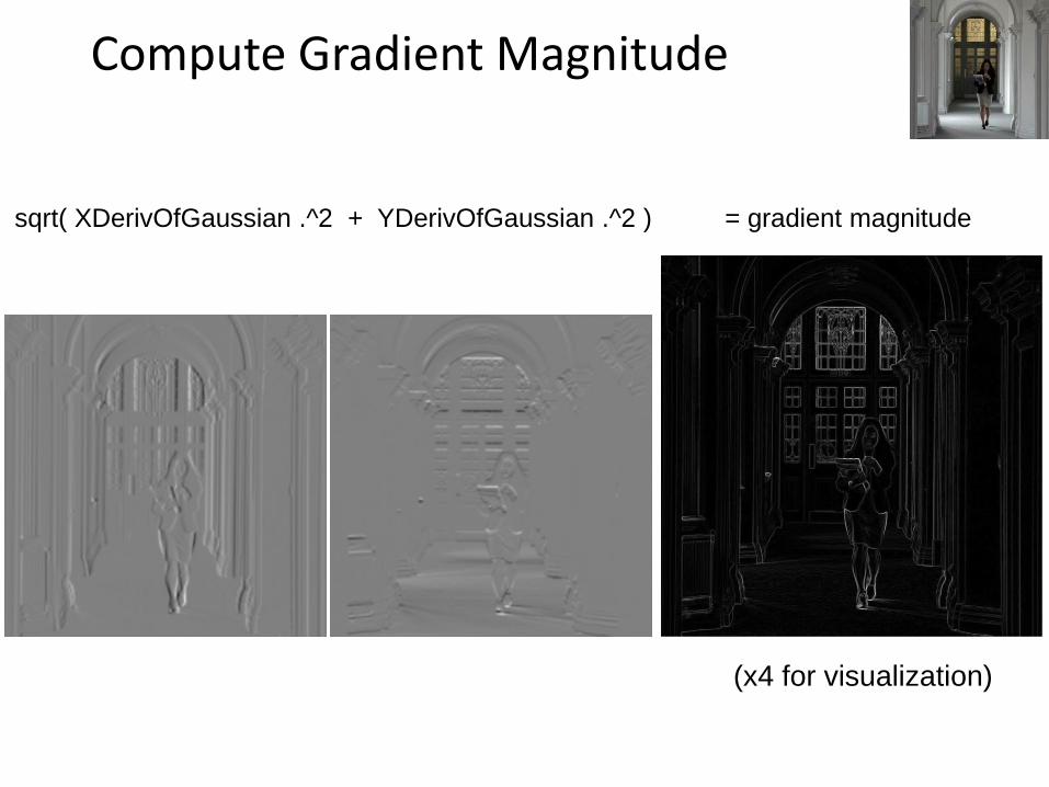
Compute Gradient Magnitude
sqrt( XDerivOfGaussian .^2 + YDerivOfGaussian .^2 ) = gradient magnitude
(x4 for visualization)

Compute Gradient Orientation
• Threshold magnitude at minimum level
• Get orientation via theta = atan2(gy, gx)

Canny edge detector
1. Filter image with x, y derivatives of Gaussian
2. Find magnitude and orientation of gradient
3. Non-maximum suppression:
– Thin multi-pixel wide “ridges” to single pixel width
Source: D. Lowe, L. Fei-Fei

Non-maximum suppression for each orientation
At pixel q:
We have a maximum if the
value is larger than those at
both p and at r.
Interpolate along gradient
direction to get these values.
Source: D. Forsyth

Before Non-max Suppression
Gradient magnitude (x4 for visualization)

After non-max suppression
Gradient magnitude (x4 for visualization)

Canny edge detector
1. Filter image with x, y derivatives of Gaussian
2. Find magnitude and orientation of gradient
3. Non-maximum suppression:
– Thin multi-pixel wide “ridges” to single pixel width
4. ‘Hysteresis’ Thresholding
Source: D. Lowe, L. Fei-Fei
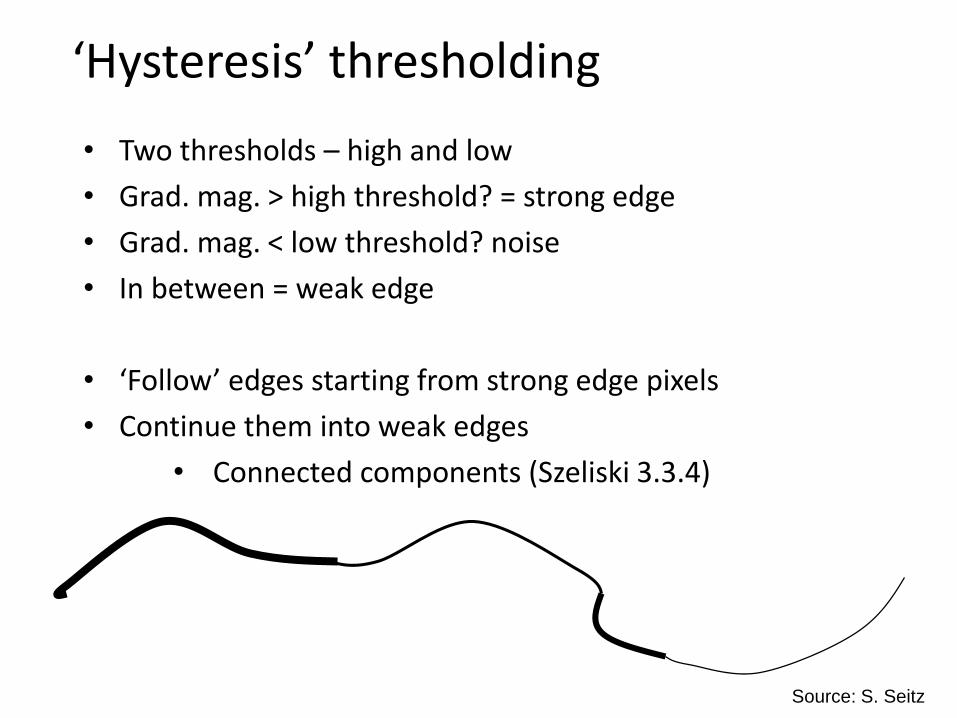
‘Hysteresis’ thresholding
• Two thresholds – high and low
• Grad. mag. > high threshold? = strong edge
• Grad. mag. < low threshold? noise
• In between = weak edge
• ‘Follow’ edges starting from strong edge pixels
• Continue them into weak edges
• Connected components (Szeliski 3.3.4)
Source: S. Seitz

Final Canny Edges
𝜎 = 2, 𝑡𝑙𝑜𝑤 = 0.05, 𝑡ℎ𝑖𝑔ℎ = 0.1

Effect of (Gaussian kernel spread/size)
Original
The choice of depends on desired behavior• large detects large scale edges
• small detects fine features
Source: S. Seitz
𝜎 = 4 2𝜎 = 2

Canny edge detector1. Filter image with x, y derivatives of Gaussian
2. Find magnitude and orientation of gradient
3. Non-maximum suppression:– Thin multi-pixel wide “ridges” to single pixel width
4. ‘Hysteresis’ Thresholding:– Define two thresholds: low and high
– Use the high threshold to start edge curves and the low threshold to continue them
– ‘Follow’ edges starting from strong edge pixels
• Connected components (Szeliski 3.3.4)
• MATLAB: edge(image, ‘canny’)
Source: D. Lowe, L. Fei-Fei
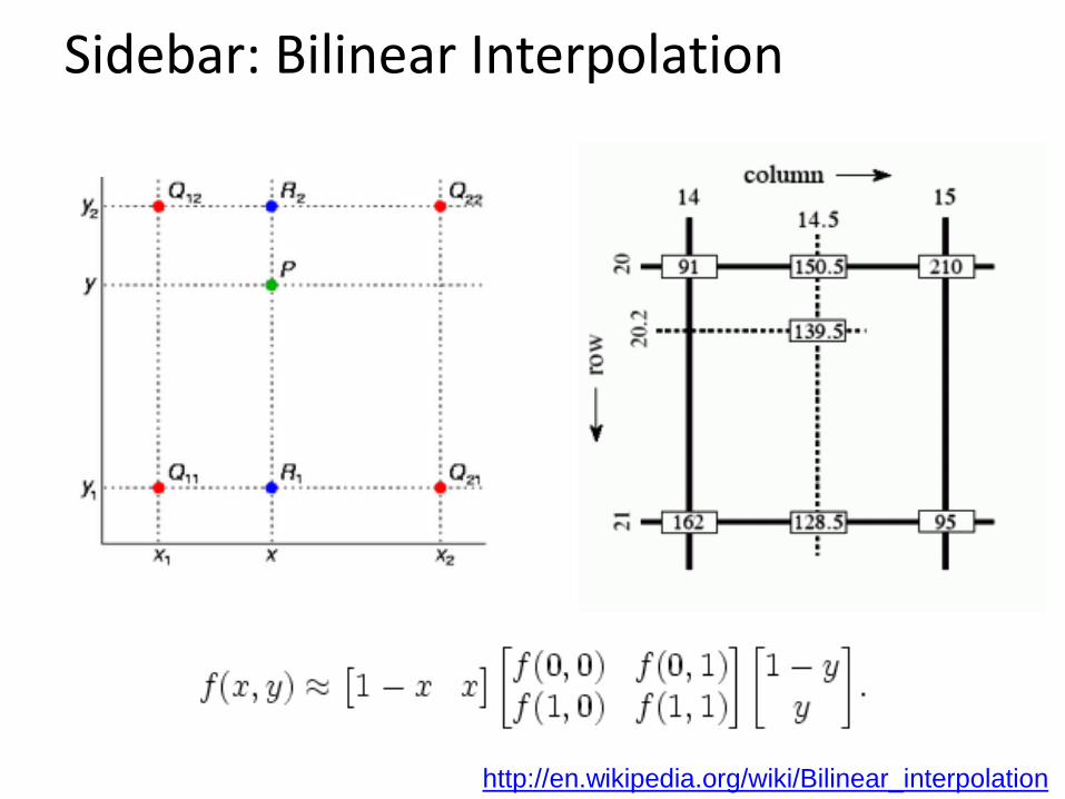
Sidebar: Bilinear Interpolation
http://en.wikipedia.org/wiki/Bilinear_interpolation

Sidebar: Interpolation options
• imx2 = imresize(im, 2, interpolation_type)
• ‘nearest’ – Copy value from nearest known– Very fast but creates blocky edges
• ‘bilinear’– Weighted average from four nearest known
pixels– Fast and reasonable results
• ‘bicubic’ (default)– Non-linear smoothing over larger area (4x4)– Slower, visually appealing, may create
negative pixel values
Examples from http://en.wikipedia.org/wiki/Bicubic_interpolation