Review of Current Air Monitoring Capabilities near Refineries in the

San Francisco Bay Area

Prepared for:

Bay Area Air Quality Management District

By:

Eric M. Fujita and David E. Campbell

Division of Atmospheric Sciences

Desert Research Institute,

Nevada System of Higher Education

Objectives

• Identify the primary risk drivers • Review and evaluate current air monitoring

capabilities. • Develop a matrix of instrumentation,

methodologies and/or other exposure assessment tools to: – enhance monitoring capabilities – provide information about emissions

• Prepare a short report describing the process used and how the matrix was developed.

Identifying primary risk drivers

Risk factors

Potential emissions

from upset conditions

Emissions from

normal operations

Chronic effects

Acute effects

Fugi

tive

em

issi

on

s

Target compounds, RELs, and monitoring methods

Open Path

500m

OpenPath

100mArea

Target

Compound

Acute

(µg/m3)

Chronic

(µg/m3) 

Photo-

metricAuto-GC

XRF tape

sampler 6 UV-DOAS OP-FTIR 7 DIAL CanisterChemically

active

adsorbent

FRM filter sampler

Passive5 lpm filter

sampler

Benzene 1300 60 0.03 3 50 3 0.06 0.3

1,3 Butadiene 20 0.02 1 10 0.04 0.03

Formaldehyde 55 9 10 10 8 µg/m3 h 0.15

Acetaldehyde 470 140 20 6 µg/m3 h 0.05

Perchloro-

ethylene 20000 35 40 0.02

Napthalene 9 0.05 2 ?

NO2 470 100 3  0.2 2 25 0.16

SO2 660 0.8 2 10 25 1.5

H2S 42 10 0.2 0.2 0.15

Ni 0.2 0.014 0.00020.26

µg/m3 h0.001

Mn 0.17 0.019 0.00030.35

µg/m3 h0.001

Cr VI 0.2

Hg 0.6 0.03 0.00020.66

µg/m3 h0.0008

As 0.2 0.015 0.00010.35

µg/m3 h0.001

Continuous

PointTime-integrated Point sample

(up to 24 hrs)

Saturation Monitoring

(7-day)

Risk Exposure Levels

(REL) 2

Time-integrated Samping

Current air monitoring capabilities • Current Air District network consists of 32 locations with 136

instruments • 20 staff in Air Monitoring with greater than $3 million in

annual operations and maintenance budget • 5 dedicated Quality Assurance staff and 7 laboratory staff

support air monitoring activities Existing air quality monitoring was designed to determine neighborhood or other EPA-defined spatial scale concentration average and range of concentrations for criteria pollutants (O3, SO2, NO2, CO, PM10, PM2.5) and certain high-priority toxics (benzene, toluene, ethylbenzene, xylenes, 1,3-butadiene, formaldehyde).

“Traditional” methods: Fixed-site Community Monitoring

Other monitoring activities

Refineries are currently required to measure H2S and/or SO2 at their fence lines: • Enforcement action can be taken on measurements • Sites are audited and data reviewed by the Air District • Additional pollutants can be monitored simultaneously

US EPA is moving to more source oriented monitoring

• NO2/CO/PM near roadway monitoring now required • SO2 monitoring may be required near sources,

depending on emissions and population • Lead monitoring required at sources emitting more than

0.5 tons per year

Fenceline monitoring

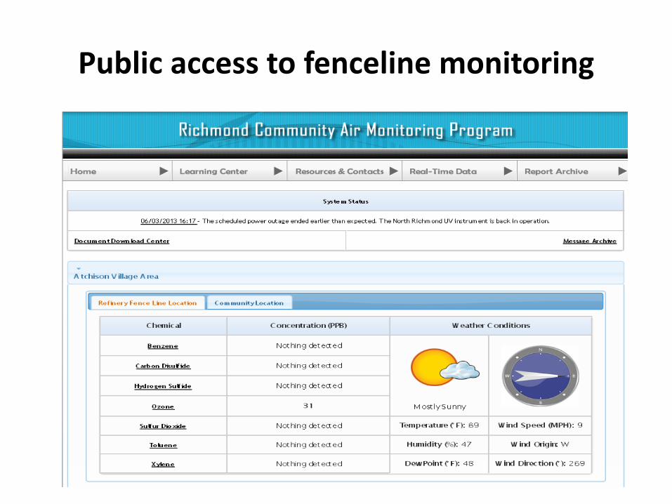
Public access to fenceline monitoring

Existing air monitoring with prevailing wind directions (West side)

Existing air monitoring with prevailing wind directions (East side)

SO2 monitoring shows concentrations well below standards at area community monitors

Primary NAAQS = 75 ppb (99th percentile) Secondary NAAQS = 500 ppb (maximum 3hr average)

Current air toxics monitoring does not show elevated concentrations near refineries,

but may not capture incidental peaks.

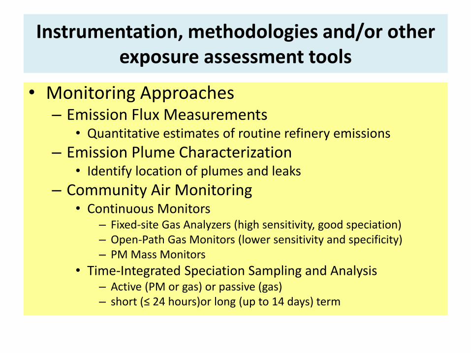
Instrumentation, methodologies and/or other exposure assessment tools

• Monitoring Approaches – Emission Flux Measurements

• Quantitative estimates of routine refinery emissions

– Emission Plume Characterization • Identify location of plumes and leaks

– Community Air Monitoring • Continuous Monitors

– Fixed-site Gas Analyzers (high sensitivity, good speciation) – Open-Path Gas Monitors (lower sensitivity and specificity) – PM Mass Monitors

• Time-Integrated Speciation Sampling and Analysis – Active (PM or gas) or passive (gas) – short (≤ 24 hours)or long (up to 14 days) term

Emission Flux Measurements and Plume Characterization

IR video cameras can locate plume source and leaks Remote Flux Measurements using

Solar Occultation or Differential LIDAR

EPA Handbook: Optical Remote Sensing for Measurement and Monitoring of Emissions Flux

www.flir.com

Continuous PM monitors

Continuous Monitors Targets MDL (1 hr)

Min Averaging Time Unit Cost Environment features/limitations

Beta-attenuation tape sampler PM2.5 2 - 10 ug/m3 1 hr $15 -20k Indoor

Federal Equivalent Method for PM10 and PM2.5. Options for low-density Teflon tape and integral nephelometer for higher time-resolution.

TEOM PM2.5 <5 ug/m3 10 min $ 30,000 Indoor Federal Equivalent Method for PM10 and PM2.5 / possible interference from ΔRH

auto-XRF tape sampler Elements K - Pb <0.5 ng/m3 15 min $ 250,000

Climate-Controlled

unique capability / high cost and unknown reliability

Aethalometer BC 0.1 ug/m3 5 min $ 20,000 Climate-Controlled

high sensitivity but non-linear response at high conc.

Photo-Acoustic Soot Spectrometer BC, PM2.5 <0.5 ug/m3 2 sec $ 30,000

Climate-Controlled absorption and light scattering

CPC UFP N/A 10 sec $ 10,000 Climate-Controlled

high sensitivity and time resolution, but no clear relationship between UFP and other pollutants or health effects

Continuous methods for monitoring gaseous pollutants

Continuous

Monitors Targets MDL (1 hr)

Min Averaging

Time Unit Cost Environment features/limitations

NO/NOx

analyzer NO, NO2, NOx <0.4 ppb 10 sec $ 12,000

Climate-

Controlled

Federal reference method / NOx produced

by all types of fuel combustion

CO analyzer CO 40 ppb 10 sec $ 11,000

Climate-

Controlled

Federal reference method / CO primarily

from motor vehicles

SO2 analyzer

SO2 or H2S or

total S <0.5 ppb 10 sec $ 11,000

Climate-

Controlled

Federal reference method, most relevant

criteria pollutant to refinery emissions

Auto-GC

Speciated VOC

<C13

<0.5 ppb

(BTEX) 3 to 60 min $30 - 60k

Climate-

Controlled

VOC speciation with high sensitivity and

specificity / complex data interpretation

UV-DOAS

NO2, SO2, H2S,

select VOC <1 - 10 ppb <10 sec

$60,000 -

200,000 Outdoor

good for detection of releases / does not

easily translate to community exposure

OP-FTIR 

SO2, CO, select

VOC 5 - 100 ppb <10 sec

$80,000 -

125,000 Outdoor

good for detection of releases / does not

easily translate to community exposure

Hypothetical comparison of reported concentrations from Fixed-site and Open-path continuous monitors

Open Path: 6.2 ppm Fixed site A: 8 ppm Fixed site B: 3 ppm Open Path: below LOD Fixed site A: 4 ppm Fixed site B: 12 ppm

Problem: • Open-path ‘fenceline’ monitors can detect peaks in

emissions, but do not provide quantitative exposure concentrations

• Fixed site continuous monitors can accurately measure ambient concentrations, but these may not reflect higher levels at other locations

Solution: • A dense array of low cost, portable samplers can be

used to determine how well fixed-site continuous monitoring represents ambient concentrations in other locations throughout a community.

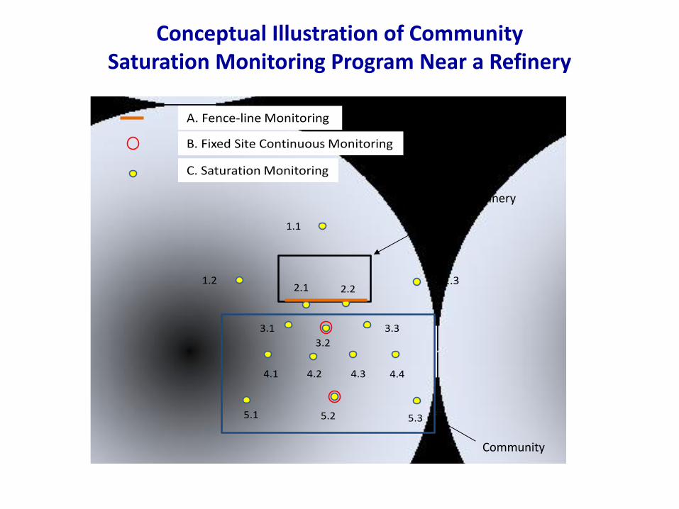
Conceptual Illustration of Community Saturation Monitoring Program Near a Refinery

A. Fence-line Monitoring

B. Fixed Site Continuous Monitoring

C. Saturation Monitoring

1.1

1.2 1.32.1 2.2

3.1

3.2

3.3

4.1 4.2 4.3 4.4

5.1 5.2 5.3

Community

Refinery

Ogawa passive samplers for NO2/NOx and SO2

(thumb size in cup shield)

Radiello passive samplers for VOC, aldehydes and H2S (size of a roll of pennies)

AirMetrics Minivol Aerosol Sampler (10” diameter x 24” tall)

12V battery or 110VAC

Samplers for Saturation Monitoring

West Oakland Monitoring

Study (WOMS)

G1

G2

G3 G4

G5

G6

G7

G8

NR1

WO1

WO2

POC

EBMUD

WO3/

CUPW

CNDW

CFDW

POU

WOMS Passive Only

WOMS Passive + PM

WOMS + PM Speciation

CASS

G1

G2

G3 G4

G5

G6

G7

G8

NR1

WO1

WO2

POC

EBMUD

WO3/

CUPW

CNDW

CFDW

POU

WOMS Passive Only

WOMS Passive + PM

WOMS + PM Speciation

CASS

Seasonal Average NO Concentrations

0

20

40

60

PO

U

G1

PO

C

G2

G3

G5

G7

G4

G6

G8

NR

1

WO

1

WO

3

WO

2

EM

UD

CF

DW

ppb

winter

0

20

40

60

PO

U

G1

PO

C

G2

G3

G5

G7

G4

G6

G8

NR

1

WO

1

WO

3

WO

2

EM

UD

CF

DW

pp

b

summer

West Oakland Monitoring Study

Incident Monitoring

• Dispersion modeling – Predict areas that will experience maximum

concentrations for different types of release and weather conditions

• Mobile Sampling – BAAQMD and/or EPA Mobile Monitoring Vans can be used

to determine areas most impacted and monitor levels

• Emerging Technology and Cooperative Approaches – highly portable, low cost monitors have potential to make

large scale saturation monitoring affordable – involve community volunteers for increased spatial

coverage during incidents

BAAQMD Mobile Monitoring Platform

Community Survey using Mobile Monitoring

Summary of Recommendations

• Verify type, location, and quantity of emissions using remote sensing flux methods • Work with refinery operators to gather this information

• Track variations in emissions via fenceline monitoring • Program already active

• Determine spatial variations in concentrations within communities using mobile and saturation monitoring projects • Use results to validate or enhance existing monitoring

• Prepare for unplanned high-level releases with dispersion modeling and fast-response enhanced monitoring protocols • Explore cooperative approaches involving community, district, and industry

Recommended methods to achieve monitoring objectives

Objective of measurement

program

Emissions Community Exposure

Characterization Surveillance Acute Effects

Routine Monitoring

Acute Effects Catastrophic

Event

Chronic Effects Routine

Monitoring

Duration days to weeks continuous continuous days Minimum of 4

weeks in 2 season

Time-resolution minutes hourly hourly varies 7 to 14 days

Location refinery boundary fenceline representative

community sites Grab sampling,

mobile sampling representative

community sites

Number of sites multiple downwind edge 1 to 3 sites multiple Multiple

("saturation")

Parameters

alkanes, olefins, CO, NH3, HCHO,

SO2, NO2,

benzene, butadiene, HCHO,

NO2, H2S all

determined by event

benze, butadiene, HCHO, NO2, H2S,

metals

Recommended Methods

SOF, DIAL flux measurements

Open-Path

photometric, auto-GC or OP, tape samplers,

met

monitoring van + canisters, med-vol

PM, OP

passive, low-volume PM