reverse small world experiment - computer science department

Social Networks, 1 (1978/79) 159-192

@Elsevier Sequoia S.A., Lausanne - Printed in the Netherlands 159

The Reversal Small-World Experiment*

Peter D. Killworth

University of Cum bridge * *

and

H. Russell Bernard

West Virginia Universityt

This paper is an attempt to examine and define the world network of a typical individual by discovering how many of his or her acquaintances could be used as first steps in a small-world procedure, and for what reasons. The town and occupation of each target was provided, together with the ethnic background, where this could not be inferred from the name. Starters were instructed in the small-world experiment and asked to write down their choice, amongst the people they knew, for the first link in a potential chain from them to each of 1267 targets. Starters provided information on each choice made (e.g. mother, cousin, friend, acquaintance, etc.) together with the sex of the choice) and the reason that choice had been made. The reason could be in one or more of four categories: something about the location of the target caused the starter to think of his or her choice; the occupation of the target was responsible for the choice; the ethnicity of the target; or some other, unspecified, reason.

Six main conclusions may be drawn from the data. (1) A mean of 210 choices per starter account for the “world” (i.e. the

1267 targets). This number is probably an underestimate. Only 35 choices are necessary to account for half the world, however. Of the 210, 95 (45%) were chosen most often for location reasons, 99 (47%) were chosen most often for occupation reasons, and only 7”/0 of the choices were mainly based on ethnicity or other reasons.

*This work was supported under Office of Naval Research Contract #NOOO14-75C-0441-POOOOI, Code 452. The opinions expressed in this paper are those of the authors and do not necessarily reflect the position of the supporting agency.

We are deeply indebted to our graduate assistant Ms. Ellen Cheung for her hetp in managing the data collection, and Ms. Regina Phillips for assistance in data colLection and for suggesting and asking the questions which led to Section Il. We are also indebted to Jack Hunter for a careful and critical evaluation of an earlier draft of this paper.

**Department of Applied Mathematics, Silver Street, Cambridge CB3 9EW, Gt. Britain. iDepartment of Sociolo~/AnthropoIo~y, West Virginia University, Morgantown, WV 26506, U.S.A.

1. Introduction

It is by now obvious that the problem of measuring social structure is an extremely difficult one. In the past decade, it seems to us that subtle and unusual techniques for data acquisition have produced more valuable information about an individual’s place in a given social group than have more traditional sociometric methods. The small-world technique, due to Milgram, is a case in point. Since Milgram’s original article (1967), a number of researchers have duplicated, verified and adapted the experiment in a variety of environments. (See Travers and Milgram 1969; Lundberg 1975; Bochner et al. 1976; Hunter and Shotland 1974; Korte and M&ram 1970.)

The small-world problem can be thought of as an attempt to define the incoming network of a preselected target person. (In this paper, ‘“network” is used to connote those people whom a person knows and can turn to for various purposes.) A group of “starters” are asked to send a folder to a target person. If the starter does not know the target personahy, then he is asked to send the folder to someone whom he believes has the best chance of knowing the target. The folder is passed along with the same instnlctions. Thus, a chain from each starter to the target is constructed. The group of

The reverse small-world experiment 16 1

people who eventually give or send the folder to the target constitutes, in some undefined way, the target’s “incoming network”.

Two things stand out in the research done in this field so far: (1) the number of links in the chains is s~~~~singly small (on average, there are 5.25 intermediaries between any two people in the U.S.); and (2) the number of people who constitute the incoming network is also small (in the 1967 experiment, for example, of the 62 completed chains, only 26 final links were required, and 3 final links accounted for nearly half the chains).

There are two good reasons not to consider the small incoming network as the target’s total (i.e., nondirectional) network. First, only 62 realizations produced the 26 final links. We can expect this number to rise as the number of chains rises; for obvious reasons, however, it should rise at an ever de- creasing rate (with respect to the number of chains) and will, presumably, asymptote to a finite value. The asymptotic value would be the target’s total incoming network; therefore 26 must be an underestimate.

Second, 26 links are too few to function as a set of paths away from a starter in a small-world experiment. We can see this very simply by em- ploying simplified forms of arguments by Pool and Kochen (1978). If each individual in the U.S. (population 2 X log) had 26 links to the rest of the world, his links would number at most (i.e. with no overlap) 26’ ; their links (same restriction applying) would be 263; and so on. This means that at a distance of 6.2 links from an individual (5.25 intermediaries yield 6.25 links), a person could contact (via appropriate chains) 7 X lo8 people. This number is clearly an overestimate on two grounds:

f 1) Whatever “structure” is, it is composed of overlap between people’s networks; an overlap ofonly 1% (so that powers rise by 0.9 at each remove) reduces the size of the contactable world to 9 X 10’.

(2) In the above calculation we have assumed that each person, at all stages of the chain, chooses the best intermediary to continue the chain. Suppose that only one “mistake” per chain occurs. This reduces the size of the contactable universe from 266.25 = 7 X lo8 to 265*25 = 2.7 X 107. Thus, even a very small amount of error has a drastic effect. In fact, allowing for one error in a mean chain length of 6.25, one would need 38 links to reach the entire United States; with two errors, this number becomes 90; and with three errors it reaches 360.

Of course, Milgram’s experiment was not designed to exhaust the target’s incoming network, but rather to find out how many links there are in the chains. But, to understand social structure, we do need to know how many links people have to the rest of the universe. There are three ways to get at this. The most obvious would be to repeat Milgram’s experiment using hundreds (or thousands) of starters. This costly and logistically horrifying modification would still yield the incoming network of only one person - the target. A way to study many individu~s’ networks is to ask people to keep track of whom they contact. Gurevich (1961) found that, on average, people come into contact with 500 other persons in a loo-day period. Of course, this does not mean that many of these contacts would be of use to

162 P. D. Killworth and H. R. Bernard

people if they were starters in a small-world experiment, but it does give an indication of the sort of numbers involved. (Pool and Kochen obtained rather larger estimates by a process of heuristic reasoning and observation.)

We wanted to design an experiment which would, hopeftllty, tell us exhaustively about many individuals’ networks. To do this, wk combined ~ilgram’s and Gurevich’s techniques to produce what we term the “reverse small-worlds” experi~nent. Instead of many starters and one tapget, we presented each starter with a long list of targets. For each target, we provided a variety of info~~~ation~ and we asked the starter to tell us to whom he would send tlle(now mythical) folder if he were initiating a small-world experiment. This experiment has the following trade-offs: all info~rlation about chain length is lost, and the experiment deals with people’s cognitive rather than behavioral networks (i.e., to whom people slr~x folders would be sent, as distinct from to whom they actually send folders). On the other hand, in a very short time a vast amount of highly detailed information can be accumulated from a wide variety of starters.

This experiment also provided a convenient way of testing whether or not people understand the size and the characteristics of their networks. Our previous studies (Killworth and Bernard 1976; Bernard and Killworth 1977) have shown that, in very limited environments, people are inaccurate in their reports of their actual communication with others. We wanted to know whether this inaccuracy extends to people’s global networks. Hence, the reverse small-world experiment was conducted.

2. The experiment

A list of targets was needed, and the list had to satisfy several requirements. First, it had to be long; but Jzow long? We wanted to provide starters with a fair number of targets from various walks of life, locations, and ethnic backgrounds; and we wanted to ensure that there were sufficient targets to exhaust each starter’s network. Gurevich’s (1961) data suggested that at least 500 would be required. Doubling this figure seemed safe.

We consulted the telephone directories of several very large cities; we matched a set of first and last names from different directories to ensure that the resulting names would be fictitious. eventually a list of 1267 was created. The first 1000 were generated to fill a matrix based on sex (male and female), race (black and white), occupation (professional, white collar, craftsman, housewife), and location (big city, small town). This last variable was subjectively operationalized; a location was classed as “big” if, in our judgement, most Americans would recognize it by name: Seattle, Tallahasee, Houston, are examples. The scale developed by Duncan and Reiss (196 1) was used to select occupations. Since a very large part of the world is made up of housewives, that occupation was assigned to 25% of the female targets. In retrospect, this was not necessary, and a greater array of occupations should be used in future experiments. In general, larger states (Illinois,

The reverse small-world experiment 163

California, New York) are heavily represented (44, 57, and 44 occurrences), while smaller states, such Alaska, Delaware, and Vermont, occur less frequently (7, 10, and 15 targets, respectively). All 50 states, plus Washington, DC (4 targets), were included in the final instrument. There were 100 “local” targets (ie., those living in areas near the starters), in this case West Virginia, Pennsylvania, and Ohio. Somewhere in the gargantuan shuffle to create the instrument, a starter got lost; this left 999.

In order to test whether ethnicity (rather than “race”) influenced people’s choices of a first link in a small-world experiment, a second list of 168 names was generated. These were clearly identifiable to most Americans as Slavic (i.e., Olga Zdrojewski), Spanish (Francisco Gonzales), Italian (Maria Vaglienti), and Oriental (Wong Fuk Lam). The 144 Slavic, Spanish and Italian names were equally divided by sex, and by “big” or “small” town. They were further divided into professionals and unskilled workers. The 24 Orientals were not divided by sex; it was assumed that most Americans could not tell the sex of, say, Wong Fuk Lam. For most purposes, black targets are treated as ethnic in what follows.

Finally, a list of 100 targets was created to represent “the rest of the world”. These are exotic names from exotic places. Only small places were used, so that starters would generally have heard of only the target’s country. The occupations of these last 100 targets were evenly divided into professionals (e.g., chemical engineer) and lower class workers (e.g., mail clerk). The first 1167 targets were presented to starters in essentially random order. The 100 “exotic” targets were left to the end. Presumably, by this time (usually several days into the test-taking procedure) starters had decided who to use for all conceivable targets in the world. As we shall show below, this conjecture was premature.

A copy of the list (a specimen page of which is given in Figure 1) was presented to each of 58 starters who were chosen to cover a wide range of social and economic backgrounds. * It is obvious from Figure 1 that the names are plausible. Until post-experiment debriefing we led starters to believe that the names were not fictitious. This was done by asking each starter to let us know if he or she actually knew one of the targets. Three starters told us they thought they knew one of the targets, but in each case they also said “it must be a coincidence” because the occupation or resi- dence was “wrong”.

All the starters lived in or near Morgantown, West Virginia. Each starter was first instructed in the small-world experiment. For each target the starter provided the name of a choice (who was known well enough to be used in a small-world experiment), the choice’s relationship (friend, mother, etc.), and

r Starters were chosen to cover a wide range of sacioeconomic backgrounds: students, housewives, blue-collar and white-collar workers, retired persons, efc. No pretense is made for representativeness - only that the sample is a representation of the locale from which it is drawn. As far as we are aware, representativeness has never been a factor in the design of sm~l-world experiments. The problem, in fact, may be intractable for reasons of practicality.

Figu

re

1.

A

spec

imen

pa

ge

of

the

ques

tion

nair

e.

542 (B) GoU.es. Wsllsce

543

Kempner, Jill

544

Disz, Ban

545

Hopkins, Barbie

546 (B) Solomen, Him1

547

Blukin, Marvin

548

Kessler, Nstthev

549 (B) Norel, Patty

550

Goltz, ssrs .I.

551

noroe, Joseph

552

Kent, Frederic

553

Dickens, Sue A.

554

Sontz, Elvis

555 (B) Numberg, Nevson

556

Pech, Melvin

557

Birbsum, June

558

McGuire, Tom

559

Digregorio,

nary

560

Evsooff. Clark

561

Puentes, ROSS

562

Paz, Ans

NAME

LOCATION

-

Corbin, KY

-

Pittsburgh,

PA

Los Angeles, CA

-

Pontiac,

IL

Aquils, AZ

-

Winchester.

TN

Harrisburg,

PA

Ainsworth,

NE

-

Huntington,

WV

Ksvsnee,

IL

Gordyce. AR

-Las

Vegas, NV

Denver, CO

-

San Jose, CA

Altooos,

PA

Albany, NY

-

Bassett, NB

Rolllog Pork, US

El Centro, CA

Portland.

OR

-

Dsllss, TX

OCCUPATION

Delivery men

Shipping

clerk

Mover

-

-

Lawyer

-

Chemical

Engineer

-

Fountain manager

Office worker

-

Eausewife

-

Claims examiner

-

_Gluer

Symphony conductor

Housewife

nsintensnce

man

Buyer

Dentist

Professor

office msnsger

Practical

nurse

Farm service vorker

Bsllerias

RACE OR

ETENICITY

Midwife

NAME

RELATIONSHIP

OTHER

a reason for making the particular choice. Four reasons were provided: location, occupation, ethnicity or race, and “other”. In other words, if the reason given were location, then sometlling about the location of the target and/or some knowledge about the location or life experience of the choice was involved in the selection of that choice. Starters were allowed to check more than one reason if they felt the need to. Ove~helmin~ly, starters chose only one reason. Where more than two reasons were checked (< 0.01% of choices), only two reasons were coded.

This provided us with two sets of data. We had a list of targets about which we knew occupation, sex, ethnicity, whether they lived in a large or small town, and location by state. Foreign countries were divided for analysis into five blocs: South America, Western Europe, Far East, Middle East, and Eastern Europe. We also had, for each starter, a list of choices (one per target) about whom we knew (a) sex, (b) relationship to starter, and (c) a reason for the starter making that choice. In addition, we also had some background info~ation on the starters (age, sex, income, religion, etc.), together with their responses to three questions which we asked 1 - 4 months after the test was over: “I-Iow many ~iffererzt choices did you make on the test?“; “Which choice did you use the most?“; “Which three choices did you use the most?“.

3. The starters

Fifty-eight persons completed the inst~Iment in 8 hours, on average. (Star- ters came to our office to take the test, but were under no time pressure. They returned as often as required to finish and were paid $30 for their participation.} Another 12 found the task too tedious and dropped out. The mean age was 36, s.d. 15. There were 34 women and 24 men in the group; 29 were married, 4 were divorced, 20 were never married, and 5 were either widowed or separated. Eighteen came from big cities, 16 from small cities, IS from small towns, and 5 were from rural backgrounds. (The city of origin of 4 starters is unknown.) Seventeen were employed full time, 20 part time, and 2 1 were unemployed. (All the unemployed were housewives, and 7 were part-time housewives.) The educational level of starters ranged widely. One completed only grade school, 6 high school, 8 completed high school and had vocationai training, 14 completed at least some college years, 16 completed an undergraduate program, 12 completed a graduate program, and one had a doctorate. Seven had a yearly income of less than $2000 (these were all students), fifteen had yearly incomes between $2000 and $5000, five from $5000 to $8000, nine from $8000 to $1 I 000, three from $1 I 000 to $14 000, four from $14 000 to $17 000, and 14 had family incomes above $17 000 per year. Thirty were Protestant, eight Catholic, three Jewish, seven ‘“other religion” (mostly foreign students), and ten professed no religion.

Starters also provided an estimate of their “ethnicity”. They created 13 categories; 40 considered themselves “American”; 18 said they were Spanish American, Black, Italian American, etc.

I66 P. Il. K~~lw~r~~~ and H. R. Bernard

Personal data were stored for each starter in the chunks as indicated here. For example, education was coded 1 - 7, from grade school to doctorate.

4. The number of choices

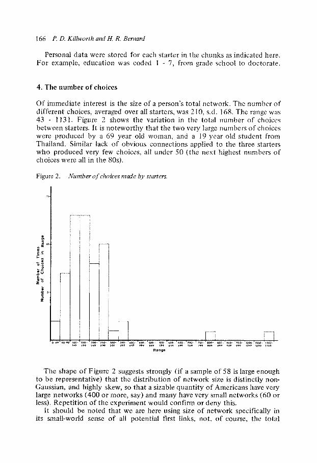
Of immediate interest is the size of a person’s total network. The number of different choices, averaged over all starters, was 2 10, s.d. 168. The range was 43 - 1131. Figure 2 shows the variation in the total number of choices between starters. It is noteworthy that the two very large numbers of choices were produced by a 69 year old woman, and a 19 year old student from Thailand. Similar lack of obvious connections applied to the three starters who produced very few choices, all under 50 (the next highest numbers of choices were all in the 80s).

Figure 2. Number of choices made by starters.

rl

The shape of Figure 2 suggests strongly (if a sample of 58 is large enough to be representative) that the distribution of network size is distinctly non- Gaussian, and highly skew, so that a sizable quantity of Americans have very large networks (400 or more, say) and many have very small networks (60 or less). Repetition of the experiment would confirm or deny this.

It should be noted that we are here using size of network specificaby in its small-world sense of all potential first Iinks, not, of course, the total


number of people known by any individual, which would be much larger, as Gurevich showed.

We can examine whether the 1267 targets have exhausted an individual’s network by plotting a cumulative histogram of the mean number (over all starters) of different choices accumulated as the number of targets increases towards 1267 (Figure 3). The gradient is almost unity for the first few targets, as each one produces a different choice, but decreases monotonically as the number of targets increases. The obvious change in gradient at 1167 results from the introduction at this point of the 100 foreign targets.

Figure 3. Cumulative histogram of the mean number of different choices accounting for a given number of targets. Error bars show one standard deviation. The change in gradient at target 1168 represents the beginning of the foreign targets. The broken curve shows the same histogram with targets 1 - 1167 in reverse order, as a test of randomness. between the full and broken curves.

t.2 u 220- cl = zoo-

5 l80-

K 160-

Y l40- LL 0 120 -

T

< __-- __--

ilk-

- indicates significant differences

d _0-- __--

2 3 200 400 600 800 1000 1200

NO OF TARGETS

Two immediate observations are possible about the curve in Figure 3. First, the error bars are enormous - because the distribution of network size is large. Second, the curve had not asymptoted to a constant value before the foreign targets were introduced. Unpleasantly, this implies that 1167 targets are insufficient to elicit the entire U.S. network of a starter. Crude extrapola- tions of the curve in Figure 3 would suggest that at least 2000 U.S. targets, and perhaps 500 foreign targets, are necessary to exhaust the network; a corresponding value of about 250 choices, plus 20 - 25 for foreign targets, would be a reasonable estimate of asymptotic network size. (Some foreign targets will be accounted for by choices who also account for targets in the U.S.). It is painfully obvious that the experiment required to produce this exhaustive network would require at least 20 hours of work by each starter.


It is possible that much of the lack of asymptote in Figure 3 was caused by the inclusion of only 100 local targets; had more been included, perhaps more of each starter’s local network (however defined) would have been produced. There is some support for this in the following statistics. The 100 local targets were accounted for, on average, by 43 (s.d. 17) different choices, whereas the 1067 nonlocal U.S. targets were accounted for by only 18 1 (s.d. 145) different choices. In other words, each local target elicited. on average, 0.43 different choices, whereas each nonlocal target only produced 0.17 different choices. These proportions differ significantly at the 1% level (although there is also significant difference between starters). This suggests that extra local targets are more likely to elicit different choices than extra nonlocal targets. However, the number involved may be small. The average overlap between the choices used for local and nonlocal targets was 27. so that the majority of the choices accounting for local targets have already been used for nonlocal targets. We shall re-interpret these figures later (Section 6).

The shupe of the curve in Figure 3 is also of interest. Since the targets are arranged randomly, it is plausible that the shape of the curve ought to be independent of the order in which the targets were presented. As a test of this, the broken line shows the equivalent curve for the U.S. targets presented in reverse order. It does not differ significantly from the original curve (recall that the standard error of the mean is a factor 58O.’ smaller than the standard deviation) except between targets 25 and 9 1, 125 and 262, where it is significantly lower than the original. This reflects the “dredging-up” phenomenon, noted by several starters: in the first few pages, they tended to “dredge up” names they had not thought of for a long time, whereas towards the end of the questionnaire this occurred rather less. It is probable that this is responsible for the lowering of the reverse curve. Apart from this effect, the strong similarity of the curves suggests that their shape is universal, at least for the sample studied.

The equivalent curve for only foreign targets rises significantly (0.1%) slower than the curve for the U.S. On average, 35 choices account for the 100 foreign targets, compared with 56 for the first 100 U.S. targets.

Is there any theoretical structure in Figure 3? This was tested by a model similar to that of Pool and Kochen (1978). The assumption is that each individual has N contacts, each of whom accounts for l/iVth of the world. A contact is chosen randomly for any target. It is then a trivial matter to produce the expected histogram of cumulative contacts, to compare with Figure 3. However, even when tuned optimally, the fit was extremely poor. Attempts to improve this by subdividing contacts into “good” and “poor” subgroups, with different proportions of network size, did not improve this. We must conclude, then, that the curve in Figure 3 is not random and does represent a facet of the starters’ mean social structure.

One can also compute how many choices are required to account for a given fraction of the world (remembering with caution the lack of any asymptote). This is shown in Table 1. Note that remarkably few choices


Table l(a). Number of choices required to account for a given percentage of the world

Percentage 10 20 30 40 50 60 70 80 90

Mean 3.2 8.5 15.5 24.0 34.2 47.2 64.0 87.0 125.4

S.D. 3.5 16.4 33.4 50.8 68.4 88.1 108.9 130.0 151.9

Table I(b). Number of choices required to account for a given percentage of the world (limiting consideration to the foreign targets)

Percentage 10 20 30 40 50 60 70 80 90

Mean 1.57 2.64 4.34 6.07 8.43 11.48 15.28 19.88 25.86

SD. 0.92 1.91 3.59 5.47 7.59 10.02 12.74 15.99 19.22

account for a great deal of the world: in particular, 34 choices account for 50%, and 125 choices (just over half the average total) account for 90% of the world. If only foreign targets are considered, 8.5 choices account for 50% and 26 for 90% of the world beyond the U.S.

The choice used most often by any starter, the “top choice’“, accounts for just under 10% of the world (the apparent discrepancy between this and Table 1 being due to the different averaging procedures used). The second- most-used choice accounts for 8%, with a gradual decline in percentage as one descends through the choices. Limiting attention to foreign targets, a starter’s (usually different) top choice accounts for 21%. The usage of the top choice wiII be examined in detail in Section 7.

The large variation in total number of choices between starters suggests that there may be systematic features in the starters’ backgrounds. Compari- son of SEC variables on starters with the number of choices they made yielded the following: only age, education and income had any effect on the number of choices. The effect of education was limited to males, and was both weak and nonlinear. Age and income together accounted for 15% of the variance in the number of choices (with a multiple correlation of 0.39*, and, analysis ofvariance showing a similar result). (Henceforth, single asterisks denote significance at the 5% level, double at the 1% level or better.) Single co.rrelations were choice-age 0.30, choice-income -0.18. In other words, older starters have more choices, except those in the higher income brackets, and the above-mentioned Thai student. Since 16% of the variance is not a great deal, there seems to be no overriding reason which accounts for the variation in the number of choices, except individu~ life histories.

5. Types of choices

Starters chose essentially three different types of people: friends, acquaintances, and family members (this latter being divided into 22 categories -

170 P. I). K~llw~rrh and H. R. Bernard

Table 2.

Variable

The number of different choices used in the given category *

~- -_____ .._

Mean

____-..-- ___

S.D.

Male friends 69 85

Female friends 42 3x

Male acquaintances 46 36

Female acquaintances 19 16

Male family 12 7

Female family 11 7

Mother 0.59 0.53

Father 0.64 0.64

Spouse 0.52 0.50

Brother 1.14 1.21

Sister 1.05 1.18

Son 0.31 0.65

Daughter 0.28 0.72

Cousin 1.3 8.2

Uncle 2.9 3.1

Aunt 2.8 2.6

Mother-in-law 0.38 0.52

Father-in-law 0.33 0.5 I

Daughter-in-law 0.12 0.38

Son-in-law 0.14 0.44

Grandmother 0.26 0.58

Grandfather 0.29 0.73

Granddaughter 0.09 0.47

Grandson 0.05 0.29

Sister-in-law 0.95 1.41

Brother-in-law 1.21 1.63

Niece 0.02 0.13

Nephew 0.55 1.39

Family 23 13

Friends 117 137

Acquaintances 10 54

P (male friends) 0.30 0.14

P (female friends) 0.20 0.09

P (male acquaintances) 0.23 0.13

P (female acquaintances) 0.10 0.06

P (mate family) 0.08 0.06

P (female family) 0.07 0.05

Males 127 104

Females 72 48

P (friends) 0.50 0.18

P (acquaintances) 0.32 0.17

P (family) 0.14 0.10

P (male) 0.60 0.10

P (female) 0.36 0.10

Friends and acquaintances 176 143

P (friends and acquaintances) 0.82 0.10

Friends/(friends + acquaintances) 0.60 0,22

*The notation P 0 indicates the number divided by the total number of choices made. (Not ail frac- tions sum to unity, owing to missing data.)

The reverse srna~~-world experiment 17 1

mother, father, etc.). The distinction between the “friend” and “acquaintance” categories was left to each starter.

Table 2 gives the mean number of choices in each category. Friends and acquaintances accounted overwhelmingly for most choices used (82%) in agreement with Travers and Milgram (1969) who found a figure of 86%. Male choices (127) were used much more than female choices (72) by both men and women starters. Nieces were hardly ever used; nephews, by contrast, were used by half the starters. Cousins were used quite frequently (over seven different cousins per starter).

Tables 3 and 4 examine how the usage of different categories of choices varied with some of the characteristics of the starters. The most important source of variation between starters was their sex. Table 3 shows the occurrences of all significant variations in usage between male and female starters.

Table 3. Significant differences in the numbers of differeent categories of choices between male and female starters*

-.. .-. Category Number used by males Number used by females Significance

Male friends 95 50 *

Male acqua~nt~ces 65 33 **

Female family 8 12 *

Acquaintances 90 56 *

Sisters-m-law 0.3 1.4 **

Brothers-in-iaw 0.7 1.6 *

Nephews 0.13 0.85 *

P (female friends) 0.14 0.24 **

P (male acquaintances) 0.29 0.18 **

P (female family) 0.04 0.08 **

Males 172 96 **

P (acquaintances) 0.38 0.29 *

P (family) 0.10 0.17 dr

P (males) 0.69 0.54 **

P (females) 0.27 0.43 **

Friends/(friends + a~uaintances) 0.86 0.80 *

*P () as in Table 2.

Males chose more males than did females (172 as opposed to 96)““. However, neither males nor females chose more females. Males were 2.5 times more likely to choose males than they were to choose females (0.69 as opposed to 0.27). However, females were not significantly more likely to choose females than to choose males (0.43 to 0.54, respectively). This con- firms, qualitatively, a result from Travers and Milgram (1969), who found that men were ten times more likely to send a document to other men than to women, whereas women were equally likely to send documents to either sex.

Clearly the sex of the target, as well as of the starter, should have a strong bearing on the sex of the choice. This is indeed the case, and will be discussed in Section 9.

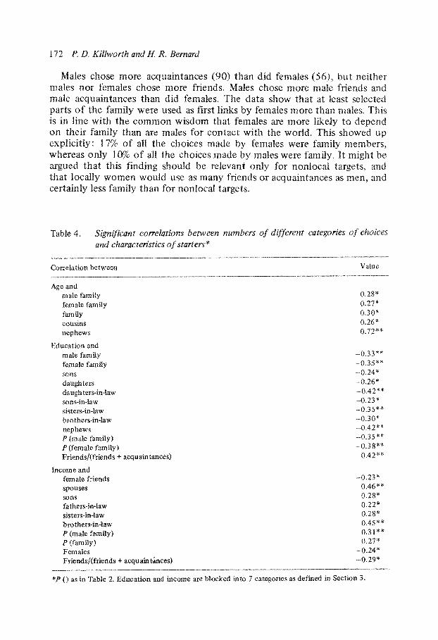
Males chose more a~q~aii~tanc~s (90) than did females (54), but neither males nor females chose more friends. Males chose more male friends and male acquaintances than did females. The data show that at least selected parts of the family were used as first links by females more than males. This is in line with the common wisdom that females are more Iikefy to depend on their family than are males for contact with the world. This showed up explicitly: 17% of all the choices made by females were family members, whereas only 10% of all the choices made by males were family. It might be argued that this finding should be relevant only for nonlocal targets, and that locahy women would use as many friends or acquaintances as men, and certainly less family than for nonlocal targets.

Correlation between Vahre l________~_~_~l__“~_- . .._ -_-..l”_--~ _____ “1--“~ -.-

Age and maie family 0.xX*

female family 0.27*

family 0.30*

cousins 0.26*

nephews 0.72””

~ducatin~ and maie family -(x33**

female family ..“0.35*”

sons -xL24”

daughters -x?6*

daughters-in-law -0.42**

sons-in-law -0.23*

sisters-in-law -0.35**

brothers-in”~aw -0.30*

nephews -0.42””

P (male fam~y) --0.35**

P (female family) .-0.38**

Friends/(friends + acquaintances) 0.42**

Income and female friends --0.23*

spouses 5.46+*

SOIlS 0.28* fat~e~-in-law 0.22*

sisters-in-law 0.28”

brothers-in-maw 0.45**

P (male family) 0.31**

P (family) 0.27”

Females -0.24*

Fr~~nds~(friends + acquaintarrces) -0.29* --__~ ll~“.-.“~--- __il _.

*P () as in Table 2. Education and income are blocked into 7 categories as defined in Section 3.

The reverse smell-world ex~e~me?lt 173

This was not the case, Certainly, women were marginally (2%) less likely to use family members for local rather than nonlocal targets. But for the 100 local targets, women still used significantly* more family than did men (25 against 15). It is not known whether this finding would hold for extremely local targets (those in the same town).

Table 4 gives the dependence of choices on other characteristics of the starters. Its results should be treated with caution, since the correlations accounted for little of the variance in the data. There was a strong tendency to choose more family members as the age of the starter increased. (Obvious correlations, such as the tendency not to choose one’s mother as one gets older, are omitted.) There was also a strong tendency to choose fewer famiIy as the education of the starter increased. Note here the strong positive correlation between education and the fraction of the starter’s friends and acquaintances which were termed “friends” by the starter. Let us call this the “friends fraction”. In other worlds, more highly educated persons tended to say that more of their nonfamily choices were their “friends” than did less-educated persons.

There was a similar tendency for starters to choose more family members (especially in-laws) as the income of the starter increased. The “friends fraction” decreased with income. (.W.B. Because of the students in the sample, the traditional high correlation between income and education was not present in the data.)

Counte~ntuitively, those who identified themselves as “American”, i.e., nonethnics, chose significantiy” more family (25) than did ethnic groups (18). The same was true for female family but not, curiously, for male family. Since six of the ““ethnic” starters were foreign students, it seemed likely that they would be less likely to use their family since they were not in their own country. Thus re-running without their data seemed likely to increase the use of family by “ethnic” starters. This was not the case, although the level of significance was reduced. It therefore appears that starters with “ethnic” backgrounds may see their families as having rather limited networks of their own. This is partially confirmed by the observation that the probability of choosing family (male family, female family, or total family) decreased monotonically with the population of the starter’s natal home. In other words, persons from rural backgrounds were more likely to choose family than were persons from small towns, and so on.

6. Individual networks

The results presented so far give little indication of exactly which of a starter’s choices are used for which targets, and for what reason. This section gives a qualitative description of a “typical” network; quantitative deduc- tions will be found in Sections 9 and 10.

A crude description of “the average network” of any starter can be made. By counting up how many times location, occupation, ethnic@ and “other”


were used as reasons for each choice, the “main” use of each choice can be obtained as the reason most used when that choice was made. Averaging this information over all starters yields an average network of:

95 (s.d. 12 1) mainly location choices. 99 (s.d. 92) mainly occupation choices,

2 (s.d. 5) mainly ethnicity choices, 12 (s.d. 25) mainly “other” choices. Judged as percentages, nearly all the average network is made up of

mainly location and occupation choices (45 and 47%, respectively). Very few (7%) choices were mainly used for any other reason.

How is the usage of these choices distributed among the various targets? A complete description is clearly prohibitive, and we shall concentrate on the eight choices used most often by each starter. (Recall from Table 1 that the eight most often used choices accounted for 20% of the targets.) It is difficult to make quantitative statements concerning the use of these choices. As an example, consider starter 1 1. His seventh most frequently used choice was almost always selected on the basis of location (55 times out of 56). On those occasions, this choice was used for targets in Washington 20 times, Oregon 33 times, and Utah twice. Clearly the choice was used overwhelmingly for just two Northwest states; the decision to neglect the Utah uses for descriptive purposes is purely subjective. Not all cases are this clearly defined; this must be borne in mind in what follows.

It is natural to begin with the most frequently used choice (the “top” choice”), quantitative details of which are given in Section 7. For 72% of the starters, the top choice accounted for a recognizable set of states when chosen on the basis of location. When this occurred, the choice was used for a wide variety of locations. For descriptive purposes, the U.S. was divided into eight blocs as defined by the U.S. Office of Education (Figure 4). The top choice of one starter was used for targets in all eight blocs; and for another, the top choice was selected for targets in six of the eight blocs. Other starters’ top choices were used for rather more restricted areas, when chosen on the basis of location (typically two to three blocs). Ten top choices were unambiguously selected for location on targets from a single state.

Top choices were less frequently selected on the basis of occupation (only by 28% of the starters). This tendency was in fact true for the eight most frequently used choices. The most popular occupation of targets for which the top choice is used was that of housewife (12% of starters). Four top choices were chosen solely for targets with other single occupations; one top choice was chosen for targets with a wide range of occupations; one was chosen for a pair of widely differing occupations; some for high-status occupations, others only for low; and so on. No recognizable pattern emerged. Some top choices were used both for targets in specific locations and targets with a specific occupation.

As one examines less frequently used choices, a tendency toward more specialized functions for the choices emerges, especially those chosen on the


Figure 4. The U.S. divided into blocs as defined by the U.S. Office of Education.

Figure 5. Number of choices, summed over all starters, which, when chosen on the basis of location, are used sole& for targets in one state, as a function of the choice number, from 1 (first most-used choice) to 8 (eighth most-used choice).

Oi I

2 3 4 5 6 7 8

CHOICE NUMBER

basis of location. As the frequency of usage of a choice decreased, the chance that that choice would only be used for targets in a single state (at least, for reasons of location) increased, at least for the first eight choices (r = 0.92**) (Figure 5). It is not known at what rank this tendency disap- pears; the labor involved in producing the subjective totals prohibits the continuance of the graph. Clearly the seldom-used choices - those used once or twice - can hardly be defined to be “single-state” in usage. However, the

degree of S~e~iaIj~ation appears to remain high for at feast the 30 most fre- ~l~~n~~~~ used chuices, as WiIl be seen shortiy.

There was no similar increase in the incidence of specialization of occupation of targets for which the less frequently used choices were selected. Indeed, the level remained roughly constant for each of the eight most frequently used choices. It may be that specialized occupation choices were used infrequently simply becatrse targets with that occupation occurred less often in the questionnaire than did targets in a specific location.

There was little sharing of f~~n~tion between the eight most frequently used choices of any starter. There was no overlap in occupation of targets (when chosen on the basis of occupation) among these eight choices; and overlay of location, when chosen on the basis of location, is mainly of the most minor kind. An example of this is starter 43. IIis top choice was used for the Far West, Rocky Mountains, South West, and Plains. this less-used choices also were used for targets in large areas of the U.S. Each of his four n~ost~L~sed choices were used for at least one target in Missouri, flowever, choice 1 was used only once for a ~isso~iri target; choice 2, three times; choice 3, seventeen; and choice 4, twice. Thus, despite the overlap, choice 3 was cIearIy the “usual” choice for Missouri. Apart from isolated cases of equaf. ‘“sharing”’ of a state between two choices, the above example represents an extreme case of overlap. For the most part, overlay did not occur.

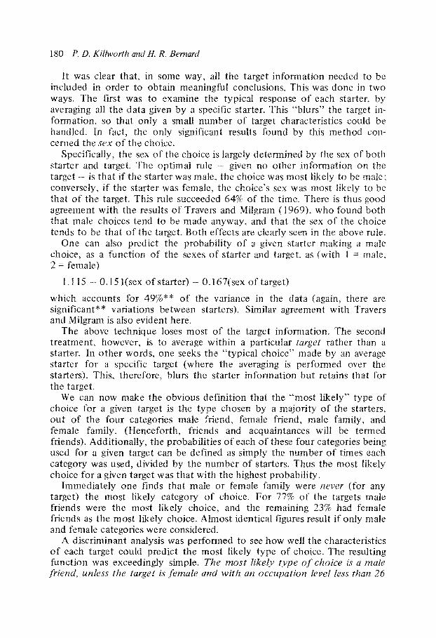
The geogra~~~~~ areas accounted for by a starter’s most-used choices are of great interest. Figures 6 and 7 show the mean fractional amount of each state accounted for by the eight most frequently used choices: Figure 6 when only choices made on the basis of location are considered, Figure 7 for ail reasons of choice. The total ~~t~~~u~~tion of a state is defined to be the number of targets in that state. The figures possess two Gomn~on features: the consistent large fraction of the Far Westerns states accounted for, and the atmost nonexistent occurrence of local states (West Virginia, Pe~~nsy~vania, Ohio), the God-~.astern states and Florida.

The latter tendency persisted even when the 35 most often used choices, accounting for over half the U.S,, were ir]G~~ld~d? aIthough it is most marked for the Iocal states (38% cover for West Virginia, 45% for Pe~lilsylvania~ compared with 60% for the others).

This suggests that the choices accounting for focaf states were used less often than those for nonlocal states. This in turn implies that the total number of different choices used for targets in a local state must be greater than the number for nonlocal states. This is confirmed by the following. Let the fraction (number of different choices on the basis of location divided by number of targets) be computed for each state. Then, although there are significant** differences between starters, the mean fraction for local states is 0.27, and for nonlocal states, 0.14. The difference is highly sig~~ifi~ant~* and shows that pro~o~io!?ally many more choices are used on the basis of location in local states.

Location need not be the reason for choice, however, far this to be the case. RecaJI from Section 4 that the mean number of choices used for the

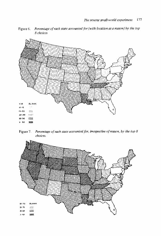
The reverse stall-world experiment 177

Figure 6. Percentage of each state accounted for (with location as a reason) by the top 8 choices

Figure 7. Percentage of each state accounted for, irrespective of reason, by the top 8 choices.


100 local targets, for any reason, was 43 ; for the 1067 nonlocal targets, 18 1. The difference in these proportions (0.43 as opposed to 0.17) is significant* *.

This shows that choices for local targets are more specialized than for nonlocal targets. However, although this implies that there is a difference between one’s local and nonlocal networks, it must be a difference in fztnction only, and not of the specific members of the networks. This is because, on average, 27 of the 43 different choices used for local targets were also used for nonlocal targets, an overlap of 63%.

The manner in which this overlap occurs, and the role of the choice involved, is clearly very important to an understanding of networks. However, such an investigation must wait until data have been collected with larger numbers of local targets, especially those in the immediate neighborhood of the starters.

7. The most frequently used choice

The choice used most frequently by starters (i.e., the top choice) has well- defined characteristics. Most were male (33); fewer were female (23). There was no tendency for males to choose a male top choice in preference to a female top choice; the same was true for female starters. Friends and acquaintances accounted for 37 of the top choices; 21 were family. This proportion is skewed towards use of family significantly** more than the overall probability in Table 2.

On average, over all starters, the top choice was used, when location was the reason, 58 times(s.d.83);foroccupation 26 times(s.d.40);forrace 3 times (s.d. 16, maximum 96); and for other reasons 38 times (s.d. 115, maximum 77 1). With the exception of the “other” category ~ due to one starter - this pattern of reasons approximately reflects those for the totality of choices.

Some characteristics of the starters accounted for significant variation in the usage of their top choices (although, again, the variance accounted for was not large in numerical terms). Female starters used their top choice significantly* * more often than did males. The usage of the top choice decreased* as the education level of the starters increased. Older people, and those from nonrural backgrounds, tended* to choose females for their top choice. All five starters from rural backgrounds used family for their top choice; this differs significantly* * from the average usage.

Starters who made fewer different choices in total tended to make male top choices (on average, those who chose males for their top choice made 168 different choices, whereas those with female top choices made 268 different choices). Male top choices were used significantly* more often for location reasons than were female top choices (82 as opposed to 30, respectively). Finally, top choices among family were used more frequently** on the basis of occupation than were friends and acquaintances (53 as opposed to 10, respectively).

The reverse small-l-world experiment 1‘79

8. Starters and reasons for their choices

This section examines the number of times starters made choices based on the four reasons offered to them in the questionnaire. On average, over all the starters, location was used as a reason 716 times (57% of the time), s.d. 3 18; occupation was used 476 times (38%), s.d. 265; race/ethnicity was used 21 times (2%), s.d. 34; and “other” was used 106 times (8%), s.d. 17 1. The percentages sum to greater than unity because more than one reason could be used per target.

lirence, overriding r~aso~s~or choice were (II vocation, and (2) occ~~ati~~. Few of the characteristics of the starters accounted for variations in the

number of times they made choices for any of the four reasons. Starters’ education level was positively correlated with the number of times they made choices based on location and ethnicity (0.22” and 0.25*, respectively), and negatively correlated with the number of choices made based on occupation (-0.25”). The only other characteristic accounting for any variation was, curiously, that part-time housewives used race/ethnicity as a reason for choice significantly* more often than full-time and nonhouse- wives (32 times per starter as against 15, on average).

In other words, the characteristics of starters do not seem to affect the reason they make their choices very strongly - indeed, the few significant correlations above would probably disappear with a larger sample.

However, there are important principles which acted to guide the way a starter selected his or her choices, and these will be discussed in the following two sections.

9. The effects of target characteristics on the types of choices made

Up to now, this paper has been essentially descriptive in nature. However, the basis of any network research must ultimately be an understanding of how a particular network unctions. In the present case, such an understanding involves, at the very least, the answers to two questions: what qualities of a target act to make a starter make a specific type of choice {e.g., male, female, friend, family, and so on)? and, similarly, what qualities of a target act to make a starter select a choice on the basis of a specific reason (location, occupation, etc.)? The latter question is examined in Section 10.

At the simplest level, one can isolate a specific target variable, e.g. its sex, and crosstabulate the numbers of various types of choices made for targets which are (in this case) male or female; this can then be repeated with the target’s size of town (little or big), occupation level, ethnicity {American or otherwise) or location (local or nonlocal). Virtually all the variance in these calculations was accounted for by variation between starters. The sole exception was that the probability of making a male choice was higher for a male target than for a female target.


It was clear that, in some way, all the target information needed to be included in order to obtain meaningful conclusions. This was done in two ways. The first was to examine the typical response of each starter, by averaging all the data given by a specific starter. This “blurs” the target information, so that only a small number of target characteristics could be handled. In fact, the only significant results found by this method concerned the sex of the choice.

Specifically, the sex of the choice is largely determined by the sex of both starter and target. The optimal rule -. given no other information on the target - is that if the starter was male, the choice was most likely to be male; conversely, if the starter was female, the choice’s sex was most likely to be that of the target. This rule succeeded 64% of the time. There is thus good agreement with the results of Travers and Milgram (1969), who found both that male choices tend to be made anyway, and that the sex of the choice tends to be that of the target. Both effects are clearly seen in the above rule.

One can also predict the ~~robability of a given starter making a male choice, as a function of the sexes of starter and target. as (with 1 = male, 2 = female)

1.115 --- 0.15 I(sex of starter) .- O.I67(sex of target)

which accounts for 49%** of the variance in the data (again, there are significant** variations between starters). Similar agreement with Travers and Milgram is also evident here.

The above technique loses most of the target information. The second treatment, however, is to average within a particular target rather than a starter. In other words, one seeks the “typical choice” made by an average starter for a specific target (where the averaging is performed over the starters). This, therefore, blurs the starter information but retains that for the target.

We can now make the obvious definition that the “most likely” type of choice for a given target is the type chosen by a majority of the starters, out of the four categories male friend, female friend, male family, and female family. (~encefo~h~ friends and acquaintances wil1 be termed friends). Additionally, the probab~ities of each of these four categories being used for a given target can be defined as simply the number of times each category was used, divided by the number of starters. Thus the most likely choice for a given target was that with the highest probability.

Immediately one finds that male or female family were IEP~Y (for any target) the most likely category of choice. For 77% of the targets male friends were the most likely choice, and the remaining 23% had female friends as the most likely choice. Almost identical figures result if only male and female categories were considered.

A discriminant analysis was performed to see how well the characteristics of each target could predict the most likely type of choice. The resulting function was exceedingly simple. The most likely type of cl-~oice is a male friend, u~zleLss the target is female and with an occupation level less than 26

The reverse small-world experiment 18 1

(which includes housewives), when a female friend is most likely. This succeeds on 81%“” of occasions; no other target variable had a significant effect. Again there is agreement with Travers and Milgram (1969).

The remarkable success rate of this (linear) prediction suggests that further improvement might be forthcoming with a further subdivision allowing for male and female starters. However, the extra scatter induced by the subdivision almost completely removes the greater accuracy in prediction (which rises slightly to 82%““). Hence, for a given target, knowing the starter’s sex ~ or any other characteristic, in fact - does not significantly improve one’s chances of predicting the most likely choice over the above rule.

The inclusion of the occupation level of target in the above rule is interesting. It can be confirmed by comparing the mean occupation levels of the targets for whom male and female friends were the most likely choices. One finds averages of 49 to 36, respectively; thus targets usually eliciting male choices do have significantly ** higher occupation levels than the remainder.

One can also fit the probabilities of choosing each of the four categories of choice, via multiple regression, Here, not surprisingly, the sex of the starter has a strong effect on the accuracy of the fits (in fact, on average, 11% of the variance is accounted for by the starter’s sex). With occupation on the Duncan-Reiss scale,

Prob. (male friend chosen) =

-0.229(sex of starter) - 0.1 19(sex of target) + 0.00 lS(occupation) f 0,907

(54% of variance)**

Prob. (female friend chosen) =

O.i06(sex of starter) + 0.1 lO(sex of target) - 0.0007foccupation) + 0.058

(32%)**

Prob.(male family chosen) =

O.O’77(sex of starter) - O.O4l(sex of target) + 0.089

(28%)**

Prob.(female family chosen) =

O.O45(sex of starter) + 0.05 l(sex of target) - O.O007(occupation) -- 0.053

(29%)“”

Although there is more scatter than in the fit for most likely choice similar tendencies can be seen: the weak probabilities for choosing family; the bias- sing of high occupations towards male choices; and, except for male family, the almost equal tendencies of sex of starter and target towards dete~ining the sex of the choice.


Thus the type of choice made can be predicted with excellent accuracy on the basis of these linear fits. Standard provisos concerning these must, of course, apply. It is possible that nonlinear combinations of target characteristics could improve on the accuracy of these predictions. However, their already high accuracy must serve as an indication that the guiding effects of starter and target sex, together with the target’s occupation level, are real effects which would persist in other more complicated analyses.

10. The effects of target characteristics on the reasons why choices were made

The previous section showed that the most likely types of choice could be well predicted from knowledge of the target characteristics and the sex of the starter. In this section the reasons starters gave for their choices are examined, and again a pattern emerges.

There were only two occasions on which a single target characteristic had any significant effect on the number of times any of the four reasons were used for a choice (with the exception of the target’s occupation level, for which see below), since the variation between starters was high. Propor- tionally, more** choices were made on the basis of ethnicity for ethnic targets than for nonethnic targets. (However, the likelihood of ethnicity being used for a reason was at all times very small.) Also, proportionally more* choices were made on the basis of location for local rather than nonlocal targets. Both findings, of course, are perfectly intuitive.

The single most important target characteristic, insofar as its effect on the reason for choice was concerned, was the occupation level. The mean occupation level of targets for which occupation was used as a reason was significantly** higher than when it was not used; significantly lower** when location was used as a reason than when not; and significantly lower** when “other” was used as a reason than when not. The target occupation had no effect on when ethnicity was used as a reason.

The strong effect of target occupation is also apparent if, in an analogous fashion to Section 9, the most popular reason for a choice is defined for each target. The most popular reason was al~a);.~ location (for 76?G of targets) or occupation (24%). Ethnicity or “other” were never the most popular reasons. A discriminant analysis showed that the most popular reason may be predicted accurately from the target characteristics for 81% of the targets by the following algorithm: For u11.v target, the most likely reuson for u choice is location, urdess the occupation level of the target exceeds X, where X is given approximately by

x=91

- 22 (for nonlocal targets) + 10 (for large town targets) - 5 (for ethnic targets)


As an example, for an ethnic target from a large nonlocal town, X would take the value 91 - 22 + 10 - 5 = 74. In other words, if such a target had an occupation level above 74, one should guess that the most likely reason for choice was occupation; below 74, guess location.

The success of this prediction (81%) is excellent, and shows clearly the relative ~po~an~e of the various target characteristics. Despite this success, however, there are clear indications that nonlinear effects are impo~ant. For instance, the sole target at occupation level 2 was most often chosen on the basis of occupation. Similarly, one of the nine targets at occupation level 96 was most often chosen on the basis of location, despite the above formula.

One can also predict, via multiple regression, the probabilities of making a choice of each of the four reasons as functions of target characteristics. This yields

Prob.(choosing on basis of location) = O.O56(size) - 0.003 l(occupation) -- 0.092 (distance) + 0.818

(37% of variance)**

Prob.(choosing on basis of occupation) = -O.O35(size) + O.O0365(occupation) -I- 0.065 (distance) + 0.109

(38%)“”

Prob.(choosing on basis of ethnicity) = O.O38(race) - 0.034

(42%)“”

Prob.(~hoosing on basis of “other”} = -0_006S(sex~ - 0.0 1 @size) - 0.05 (occupation) - 0.0 12(race) + O.O25(distance) + 0.10

(17%)“”

where size = 1 for small and 2 for large towns, distance = 1 for local and 2 for far towns, and race = 1 for American and 2 otherwise. All these fits, apart from “other”, account for a large amount of variance, although all under 50%. From this, the archetypal “location” target would be in a local large town with zero occupation level (0.82 probability), and the archetypal “occupation” target is a far, small town with maximum (100) occupation level (0.57 probability). This is in good agreement with the previous discriminant analysis. Note also that including starter characteristics gave no improvement to any of the fits.

Much of the scatter in the regression analyses comes, oddly enough, from different probabilities of making a choice with a given reason for targets whose characteristics are effectively identical. If one further averages over each occupation level, to produce the probability of making a choice on the basis of occupation, as a function solely of the occupation level of the target, Figure 8 emerges. Again, the probability of using occupation as a reason


increases strongly (Y = 0.68”“) with the occupation level of the target.* (The peak at level 42 is “photographic processor” ; choices were made on the basis of occupation on 70% of occasions for this target.)

Figure 8. Mean probability of a starter making a choice on the basis of occupation as a function of the occupational level of the target on the Duncarz-Reiss scale. The straight line shows the best fit, accounting for nearly half of the variance.

Limited confirmation for these results comes from Travers and Milgram (1969). The target in their small-world experiment was a stockbroker (85 on the Duncan-Reiss scale). The best-fit line and, coincidentally, the data, in Figure 8, give a probability of 0.5 of making a choice on the basis of occupation when the target is at occupation level 85. Using the numbers of the links in the “stockholder group” and “random group” of chains who reported employment connected with finance (which we interpret as a choice on the basis of occupation) given by Travers and Milgram, a value of 48% or 46% is obtained for the probability of an occupation-oriented choice. (Their text is not totally specific as to whether their proportions applied to complete or incomplete chains, hence the uncertainty.) Thus these empirical values of Travers and Milgram (1969) are in excellent agreement with our predictions.

In fact, the agreement is even better if the multiple regression fit is used to distinguish between the location of the targets. For a U.S., large, nonlocal town stockbroker (used by Travers and Milgram for the figures just quoted) one obtains a probability of 0.48. It would be interesting to compare their

20ther correlations between reason and occupational level were: with location, --0.59**; with

race, 0.02; and with “other”, -0.53**.


figures for the Boston (local) chains, when a probability of 0.42 is predicted. Unfortunately, Travers and Milgram ( 1969) give no equivalent data.

The conclusion to be drawn from this is that, overwhelmingly, the pre- dominant feature of the target which determines which reason for choice will be used is the status of the target’s occupation: if high, the choice will probably be made on the basis of occupation, if low, on location.

A qualitative note is in order about choices on the basis of “other”. From inspection of the data, “other” appears as a weaker variety of location. For targets of a medium occupation level in a given state, choices were mostly made on the basis of location. For lower status targets, the same choice tended to be made, but with the reason given changed to “other”. We believe that this effect occurs because starters do not wish to associate their choice with too low a status target, and hence invent, in their own minds, another reason for making the choice. We stress that this is a qualitative interpretation only, there being no obvious way to quantify it.

One’s man in...

The above calculations may well have brought to many reader’s minds the well-known phrase “my man in...“3 where the blank is filled in with some location. Whether starters have “their man in...” can be tested, and even a (reasonably) precise working definition can be formulated, as will now be shown.

To begin with, Section 6 showed that on virtually no occasion was an entire state accounted for by a single choice. One can, therefore, ask two distinct questions. First, how many different choices were required to account for all targets in any given state when location was given as the basis for choice (i.e. what is the variety of choices)? On average, any one choice accounts for three targets in any state; the number of targets accounted for increases weakly with the distance from Morgantown, West Virginia. (Distance is defined to the center of the state in question, and measured, lacking any more accurate measures, in centimeters on a map. Alaska and Hawaii are purposely omitted.) This suggests, weakly, that one tends to have a “man in” states further from home.

The second, more relevant, question is: how much of a given state is accounted for by the “best” single choice (i.e., the choice accounting for the largest number of targets in that state, when chosen on the basis of location)? ‘The restriction to location choices is a weak one; as seen earlier, three- quarters of choices are made on location, and the remainder are mainly for high-status targets.

- 3We were concerned about the connotation of the phrase “your man in Idaho”. Aside from the fact

that this rather sexist phrase is a common expression in English, it also turns out that the people who

handle a particular state are males much more than they are females (62% vs. 38%). This appears to be an extension of the finding that more male choices are made anyway (64% vs. 36%).


On average, the “best person” for any given state accounted for 69% (s.d. 9%) of the occurrences of that state in the questionnaire, when choices were made on location. This figure is both surprisingly high and surprisingly uniform, and suggests that a working definition of “a man in...” can be found, as follows.

We define a choice to “handle” a state (i.e., to be “a man in...“) if that choice accounts for two-thirds or more of all the targets in that state when chosen on the basis of location. Then the mean number of states, for any starter, which are each “handled” by a single choice is 24.9 (s.d. 8.8). Put another way, 49c/0 (s.(I. 17%) of’ all states in the U.S. are handled by (I (usuully different) single person.

Figure 9. Fractional amount of each state accounted for by the optimal choice for each state, as a function of distance from Morgantown (the units are cm on a map in a telephone directory).

PL’ ‘3 9 8 a ‘8 8 I m ‘I’ 8 a J 0 I 2 3 4 5 6 7 8 9 IO II I2 I3 14 15 16 17 DISTANCE FROM MORGANTOWN

The distribution of “handled” states is not uniform over the U.S. Figure 9 shows how much of each state is accounted for by the “best” choice for that state, as a function of the distance of the state from Morgantown. Although the correlation is not significant, the impression one gets is of low amounts accounted for in local states (West Virginia, Pennsylvania, Ohio) and almost uniform amounts (about 70%) for other states, independent of distance, as indicated by the superimposed lines. California is a notable exception.

Finally, although there are insufficient targets to enable firm statements to be made, one can examine the parallel concept of “one’s -” (high-status occupation). The restriction to high status is necessary, as we have seen that occupation-based choices are mainly made for high-status targets. The number of different choices used for targets in a given occupation level (usually unique occupations at high levels) declines strongly (r = -0.41**)

with occupation level. Thus one uses fewer choices for targets of a given occupation as the occupation status rises. However, the numbers of high- status targets are too few to allow more statistically significant statements to be made on this point.

11. Accuracy of starters

As noted in Section 2, starters were asked, some months after they completed the questionnaire, how well they recalled their answers. Although posed as a test of recall, we prefer to think of this as a test of how well starters understand the network in which they are embedded. This is a valid comparison provided (a) that a starter’s world network is changing at a sufficiently slow rate and (b) that the picture of the network emerging from the data is a me~~gful one. With these assumptions, it follows that if a starter understood his network at the time he completed the questionnaire, he still understood it when asked about it later. Furthermore, what he understood was essentially the same as when he provided the data about it.

Therefore it seems relevant to enquire how well his understanding of the network agrees with what the network actually looks like. As a simple measure, starters estimated how many different choices they had used. The answers obtained (from 40 starters) are summarized in Figure 10. In only one case did a starter overestimate, and then by only 1%; the starter concerned was associated with the researchers, a trait which clearly improved starters’ powers of estimation.

In general, starters guessed that they had used an average of about SO choices. This is about one-third the actual total for the group concerned. In no case was a guess larger than 200 made. There is a positive correlation of 0.33* between correct and estimated number of choices, which at least indicates that guesses of network size do tend to increase with network size. However, the consistent and blatant underestimates suggest that starters have no real idea of the size of their networks.

There is a plausible reason for this. As was seen in Section 6, choices which handle local targets are not frequently used in the questionnaire; yet in day-to-day existence these choices are usued continually. We suspect that the top 35 choices, although they accounted for half the U.S. for most starters, are so infreqLlently used in practice that starters simply forgot about them when answe~ng our question.

Indications of this also come from the responses to “who are the three choices you used the most?“. (The similarity between this question and the traditional sociometric question is deliberate.) Surely, we felt, starters ought to be able to name, say, their most frequently used choice. After all, that choice accounted, on average, for 10% of the targets. Unfo~unately, this was not the case.

On average, starters only guessed the name of their most frequently used choice 43% (s.d. 50%) at the time. A similar pattern emerges if one examines

188 P. D.

Figure 10.

iooc

8OC

‘i; . -0’ 4oa f 2

7 ; u

200

*- l .

:

. **. .

l .

_,-Line of Equality

. . --K l

‘... . . n .-L _---- . . . . . Cc-

. 0. . n /---- . . .: l

N--c

-/-- f-/-

-I-

rC-- ! I ,

100

Number of Choices Estimated

I 200

how many of the top three choices were correctly identified~ irrespective of order. (This is the A score of Killworth and Bernard (1976a).) The mean score was 1.4, s-d. 1, so that only one-half of the most frequently used network is identified correctly; we suspect that this is for the same reason as given above.

It was possible that one or several of the starters’ characteristics could account for the variation in accuracy, although this seemed unlikely from our previous results (Bernard and Killworth 1977). However, it turned out that one characteristic did account for some of the variation of accuracy: if the starter was in part-time employment, his accuracy was low; if in full- time employment or unemployed (for whatever reason), his accuracy was high. As confirmation, this also showed up in the “housewife” subcategory of “part-time housewife”. We are at a loss to explain this, unless it reflects a genuine difficulty of the part-time employed to handle different networks - work, home, friends - in what must be rapid succession in day-to-day life.

By an unfo~unate oversight, the length of time between a starter com- pleting the questionnaire and his being asked to recall his top three choices

The reverse ~al~-~r~ experiment 189

was not recorded. Hence we cannot compute whether there is a deterioration in recall with time. However, in many other experiments (Killworth and Bernard 1976a; Bernard and Killworth 1977) we have found that informants’ accuracy in recall of their communication (in both open and closed networks) was unreliable even when tested just after the period of communication. Given also that we should expect a starter’s global network to be fairly stable with time, there is no a priori reason to suppose that starter inaccuracy in this experiment is a function of the relatively short (1 - 4 months) time between questionnaire and recall.

We are thus forced to con&de that the level of starters’ accuracy is low, by which we mean that their recall is sufficiently inaccurate to rule out any meaningful use of the recall ~fo~ation for any other purpose save the above comparison. Whether the accuracy would rise if the questionnaire had been unbalanced by the addition of many more local targets must await further experiments.

12. Conclusions

This experiment was designed to examine people’s cognition (or guesses) about how they would behave under specified conditions. The object was to describe the incoming network of a group of persons, i.e., their set of first- step connections in a small-world problem. The very large amount of data generated by our technique allowed us to make many strong statements about the shape of the incoming network. However, there are drawbacks in the technique, and our conclusions are by no means secure.

(1) This is the first iteration of this experiment. It is based on only 58 starters, all of whom live in Morgantown, West Virginia. The limitations on inte~retation of our findings are obvious.

(2) Many of our most potent findings are based on excellent linear fits to the data. However, there may exist better nonlinear fits - we just don’t know.

(3) The specified behaviour which we were simulating (the small-world problem) never occurs except when social scientists create it. This creates obvious limitations, insofar as generalizing from these data is concerned, but these limitations are no more or less stringent than those which must be imposed on any other fomr of sociometric research. Ultimately, we want to understand social structure, here defined as the pattern of overlap both between informant’s cognitive networks, and between their behavioral networks. The reverse small-world experiment provides a very rich source of data on people’s cognitive networks.

(4) The experimental design itself, with hindsight, could have been better. Many more “local” targets should have been included. Starters frequently told us that they “never got a chance to use” many of their acquaintances who lived nearby. In future experiments all important personal data about the choices (their occupation, precise location, age, etc.) should be collected.

As it stands now, we cafl’t tell whether someone’s “man in Idaho” actually lives in Idaho. In future experiments, larger and more representative samples of starters should be used,

(5) Perhaps the greatest “drawback” is caused by the sheer size of the data. Ideally, one would like to create a mean “cognitive map:’ of all the residents in the U.S. for which the first 1167 targets serve as proxy. What in general makes some targets seem like others to starters? There is an obvious taol to answer this question: multidimensional scaling (MDS). It is quite

Figure 11_ Results of multidimensional scaling analysis on rhe first 100 targets. S;imi- larity coefficients are proportional to the number of times the sume choice uws used for any pair of targets. Under&es indicate an occupatioia level of between 70 - 79; a box indicutes u level of80 or above. The sole West Viv&niiz entry is otltside the normal bo~i~~ds of the rou&e, as showrr b~p the superimposed bo~~~rie~

FL .L

OR UY

RR

1R UFi

RR %i

NV blY

SD

WC0 @NV

NH

TX VT TX

TX #?

The reverse shall-work experiment 19 1

strai~tfo~ard to generate a matrix of similarity coefficients between targets (a count of the number of times the same choice is used for each pair of targets will do). Then anMDS would yield subgroups of the targets which are perceived as similar, and conclusions could be drawn from these groupings. Unfortunately, the size of the matrix concerned (over lo6 entries) prohibits this analysis on present computers.

However, as an indication of the potential results, we have performed such a calculation with the first 100 targets only (requiring less than a minute on an IBM 370). The result is shown in Figure 11 and has been suitably rotated to maximize its similarity with a genuine map of the U.S. Note the misplace- ments of California (not controlled by any one choice) and Texas. The South, New England and Far West states are basically placed correctly. Note also how the use of occupational choices (cf: Section 10) causes a drift of high-status targets towards the edge of the diagram. It is also interesting to compare Figure 11 with the mental maps of the U.S. by Gould and White (1974). Even with only 100 targets, enough structure is revealed to indicate that an MDS on all 1167 targets (or even, intriguingly, to include the foreign targets) would be extremely interesting.4

Were it not for Milgram’s original experiments, this research would have to apply only to cognitive processes. However, the strong similarity between predictions from some of our results and the results of Travers and Milgram (1969) does suggest that the reverse small-world experiment is an adequate proxy for behavior. Two points bear directly on the comparison between the experiments. First, in our experiment starters were not required to mail anything to their choices. In many cases starters reported that they were unsure of the current address of some of their choices. The instructions for the experiment only specified that starters (a) know their choices well enough to ask them to participate in a small-world chain; and (b) that they be able to contact their choices if necessary. We suspect that there would be a great tendency to restrict the number of choices used in an experiment where actual contact with choices was involved. This restriction would favor the use of choices people know best. Furthermore, in our experiment, some starters tried to “use as many different names as possible”, in spite of repeated instructions that this was not necessary.

Another feature of the reverse small-world experiment is that the most frequent choices did not necessarily appear early in the responses to the questionnaire. As an indication, on average 12.3 (s.d. 3) of the 20 most frequently used choices were not among the first 20 choices triggered. There

4Gould and White, of course, measured geographic preferences rather than people’s cognition regarding who they know in various regions. As a starting point for further research, it would be interesting to know if the shape of preference maps is similar to, or is a function of cognition, regarding who people know. For example, in alI areas of the U.S., Gould and White’s informants agreed that the Dakotas were of very low prestige (Gould and White called it the “Dakota sinkhole”). Califor- nia was univer~y thought “well off”. West Virginia was universally thought “badiy off”. Do people say they know more (of higher occupation level) persons (ie., choices) in high-prestige states? The possibilities are very interesting.

are two possible reasons for this. First, the order of the targets may not have been sufficiently random. However, recall that reversing the order of the targets produced no significant difference. This, therefore, suggests that the second explanation is more likely to be correct. This is that people get accus- tomed to the experiment as they get deeper into it. In fact, several informants said that the first 10 pages or so of the questionnaire helped to get them “warmed up” to the task of selecting appropriate choices. Of course, this was precisely the point of the technique.

The result of this is that “more appropriate” choices may tend only to be triggered long after the beginning of the questionnaire. If this is true, it suggests that single realizations of small-world ex~~eriments may be generati~lg a behaviorally biassed picture of people’s cognitive network. This, of course, is the direct opposite of the possibility, noted above, that the reverse small- world experiment may be generating a cognitively biassed picture of the behavioral world. As we have shown elsewhere (Killworth and Bernard 1976b), there are probably two quite distinct “social structures” based on cognition about one’s place in a network and one’s actions within that network. Exactly how the discrepancies between these two networks are handled by individ~~als urgently needs research.

References

Bernard, II. R, and P. D. KiJlworth 1977 “informant accuracy in social network data II”. Huma?? ~o~l~~utli~atiol~ Research 4:3--l 8.

Bochner, S., A. Buker and B. M. McLeod 1976 “Communization patterns in an international student dormitory: M~ification of the

smalJ world method”. Joum~t of Applied Social Psychology 6:275-290. Duncan, O.D.

1961 “‘Socioeconomic Index scores”. In A. J. R&s, Jr. (ed.), Occupations and Social Status. New York: Free Press.

Gould, P. and R. White 1974 MentalMaps. Harmondsworth: Penguin.

Gurevich, M. 1961 The Social Structure of Acquaintanceship Networks. Ph.D. Dissertation, MIT, Cambridge.

Hunter, J. E., and R. L. Shotland 1974 “Treating data collected by the ‘small world’ method as a Markov process”. Social Forces

52:321--332. Killworth, P. D. and H. R. Bernard

1976a “Informant accuracy in social network data”. Human Organizaiion 35:269-286. 1976b “A comparison of structure in behavioral and cognitive social network data”. Technical

Report No. KB-113-76. Office of Naval Research, Code 452, Arlington, Virginia. Korte, C. and S. Milgram

1970 “Acquaintanceship networks between racial groups: Application of the small world method”. Journal ofPersotzality and Social PsychoIogy 15(7):101-l 18.

Lundberg, C. C. 1975 “Patterns of acquaintanceship in society and complex organization: A conlparative study

of the small world problem. Pacific Socio~~gi&al Review 181206-222. Mitgram, S.

1967 The small world problem. Psychology Today i :6 167. Pool, I. de S. and M. Kochen

1978 “Contacts and influence”. Social Networks 1~5-52. Travers, J. and S. Milgram

1969 An experimental study of the small world problem. Sociometry 32:425443.

reverse small world experiment - computer science department

Documents