Retail Markups and Discount-Store Entry

Lauren Chenarides, Miguel Gomez, Timothy J. Richards and Koichi Yonezawa�

April 6, 2021

Abstract

�Hard discounters�are retail formats that set retail food prices even lower than ex-isting discount formats, such as Walmart and Target. O¤ering limited assortments andfocusing on store-brands, these formats promise to change the competitive landscape offood retailing. In this paper, we study the e¤ect of entry of one hard-discount formaton markups earned by existing retail stores, focusing on several important grocery mar-kets across the Eastern U.S. Focusing on establishment-level pro�tability, we estimatestore-level markups using the production-side approach of De Loecker and Warzynski(2012). We �nd that hard-discounter entry had the expected e¤ect of reducing marginsfrom similar stores, but did not a¤ect markups earned by stores in the same market thatare likely to appeal to a di¤erent market segment. In general, hard-discounter entryreduced markups for incumbment retailers by 7:3% relative to markups in non-entrymarkets. *These results indicate that the net e¤ect of hard-discounter entry reducesthe overall level of store pro�tability, regardless of higher sales realized by incumbentretailers.*

Keywords: Discounters, food retailing, markups, retail pricing, production economics.JEL Codes: D43, L13, M31

�Chenarides is Assistant Professor and Richards is Professor and Morrison Chair of Agribusiness, MorrisonSchool of Agribusiness, W. P. Carey School of Business, Arizona State University; Gomez is Professor andYonezawa is Research Associate, Dyson School of Applied Economics and Management, Cornell University,Ithaca, NY. Contact author: Richards, Address: 7231 E Sonoran Arroyo Mall, Mesa, AZ, 85212. Ph. 480-727-1488, email: trichards@asu.edu. Copyright 2020. Users may copy with permission. Funding fromAgriculture and Food Research Initiative (National Institute for Food and Agriculture, USDA) grant no.2019-XXXX is gratefully acknowledged.

1 Introduction

Hard-discounters, generally de�ned as retailers that o¤er limited assortments, high-quality

private label brands, and prices that are often 40% � 60% lower than current �discount�

retailers, are an emerging format in the US market (Vroegrijk, Gijsbrechts, and Campo

2013, 2016; Progressive Grocer 2019). In fact, two hard discounters, Aldi and Schwarz

Group (parent of Lidl) both accounted for over $100:0 billion in sales in 2017, and each had

nearly three times the compound annual growth rate between 2012-2017 as any other store

in the global top-10 (Steenkamp 2018). Although Aldi has been in the US market for over 20

years, the hard-discount concept has only recently emerged as a clear competitive threat to

existing food retailers. Despite the potentially transformational nature of the hard-discount

business model, there is very little empirical research of their impact on existing retailers. In

this paper, we provide empirical estimates of the e¤ect of hard-discounter entry on incumbent

retailer markups, and store pro�tability.

Estimating the impact of hard-discounter entry on retail markups is not just a matter

of curiosity. In recent decades, there have been a number of entry �waves� from retailing

formats that seek to capitalize on the relatively large sales volumes associated with selling

food. For example, in the 1990s, Walmart expanded from its base in Bentonville, Arkansas, to

occupy nearly every market in the US, and many markets overseas. The impact of Walmart

entry has been dramatic, and well-documented (Singh, Hansen, and Blattberg 2006; Basker

and Noel 2009; Zhu and Singh 2009; Ailawadi et al. 2010; Courtemanche and Carden 2011;

Holmes 2011; Huang et al. 2012; Iacovone, et al. 2015; Arcidiacono, et al. 2016; Atkin, et

al. 2018). In the 2000s, existing retailers consolidated in the face of Walmart entry, and club

stores became the latest competitive threat (Courtemanche and Carden 2014; Bauner and

Wang 2019). In the 2010s, online shopping emerged, but did not become a force for change in

the grocery industry until Amazon acquired Whole Foods in 2017 (Turner, Wang, and Soper

2017), and the Covid-19 pandemic of 2020 accelerated the move online by some 10 years

relative to existing trends (Progressive Grocer 2020). Currently, European hard-discounters

are entering many key markets in the US, and hope to succeed by providing essential items at

prices even lower than Walmart or club stores (Jackson 2020). Understanding the impact of

1

entry on incumbent retailers, therefore, is critical both for retail practice, and for developing

fundamental knowledge regarding the forces that shape US retailing.

Researchers generally examine the impact of entry using traditional, demand-side meth-

ods, combined with counterfactual simulations. However, estimating the e¤ects of entry

using store- and �rm-level markup data is arguably more relevant as the average food re-

tailer carries thousands of products (FMI 2021). Moreover, consumers often do not recall

individual item prices (Dickson and Sawyer 1990; Loy, Ceynowa and Kuhn 2020), but rather

basket-level prices (Bell and Lattin 1998), or �rm-level product aggregations (Blonigen and

Pierce 2016). Markups are of central concern to retailers because of their implications for

pro�tability, and to policy makers dues to their consequences for price-setting conduct and

industry competition. For these reasons, we examine the impact of hard-discounters�entry

into several important US grocery markets on using a store-wide, markup-based approach.

We are not the �rst to consider the competitive e¤ects of hard-discounter entry, and the

nature of competitor responses. For example, Vroegrijk, Gijsbrechts, and Campo (2013)

argue that hard-discounters may have a �complementary�e¤ect on existing retailers, as con-

sumers tend to seek out the lowest-cost source for price-sensitive items, while seeking out

traditional retailers for categories in which variety and quality may be more important. In a

study most similar to ours, Cleeren et al. (2010) examine the inter- and intra-format e¤ects

of entry between hard discounters and supermarkets in Germany. Focusing on �rm-level

outcomes, they �nd a signi�cant threshold e¤ect for the impact of hard-discounter entry

on supermarket pro�ts. In terms of incumbent responses, Lourenço and Gijsbrechts (2013)

suggest that the optimal response by incumbent retailers to hard-discounters�attempts to

take away market share in the national brand market is to introduce only category-leaders,

and at prices that re�ect favorable value-for-money relative to their traditional-supermarket

competitors. Similarly, Vroegrijk, Gijsbrechts, and Campo (2016) examine whether intro-

ducing low-price private labels may be an e¤ective way of beating hard-discounters at their

own game, �nding only limited success, while Hökelekli, Lamey, and Verboven (2017) sug-

gest that price-competition through standard private labels may be the least-bad defensive

strategy in the long run. While these studies provide valuable insight on the reasons why

hard-discounters may co-exist with traditional retailers in the same markets, they do not

2

quantify the ultimate impact hard-discounter entry is likely to have on incumbent markups,

and focus on empirical evidence from only a limited number of product categories.

Beyond the speci�c example of hard-discounter entry, and the evident importance of �rm-

level pro�t, we know surprisingly little about retailing markups in general. Conventional

wisdom holds that the retailing sector is very competitive (Bersteanu, Ellickson, and Misra

2010; Ellickson 2016), with net margins averaging 2:0% according to industry �stylized facts�

(Campbell 2020). However, estimating markups at the store level is a di¢ cult empirical

problem. The typical approach to estimating market power in retailing relies on demand-

side methods (Berry, Levinsohn, and Pakes 1995; Nevo 2000; Chintagunta 2002) wherein

the researcher estimates a large matrix of own- and cross-price demand elasticities, which

condition the retailers�ability to achieve an equilibrium price under some assumed form of

an oligopolistic pricing game. However, more recently, others recognize that if the goal is to

estimate �rm-level markups, then starting from a highly disaggregate set of products is not

necessarily the most e¢ cient way to begin, and a very restrictive one at that. De Loecker

(2011), De Loecker and Warzynski (2012), Traina (2018), and many others, approach the

problem of markup estimation instead from the production side, applying the insight of Hall

(1988) that markups can be estimated from a simple condition on the output elasticity of a

variable input, and input-expenditure shares of that input. While most applications are in

trade (De Loecker 2007; Klette 1999) and macroeconomic markup estimation (De Loecker,

Eeckhout and Unger 2020; Traina 2018), this approach is also useful in uncovering markup

patterns among food retailers. We provide new evidence on the relative competitiveness of

food retailing, and examine the speci�c case of how market-entry by a discount-retail chain

a¤ects markups of incumbent retailers, by estimating store-level markups from a production-

side perspective.

Our conceptual approach is well-understood. Extending the growth model of Solow

(1957), Hall (1988) shows that �[U]nder competition and constant returns, the observed

share of labor is an exact measure of the elasticity of the production function...�so any de-

parture between these two measures, assuming constant returns, is interpreted as a measure

of imperfect competition (p. 923). De Loecker (2007), De Loecker (2011), and De Loecker

and Warzynski (2012) develop the econometric details of how this conceptual model can be

3

used to test for departures from competition in �rm-level data, but the underlying logic is

the same: With only limited �rm-level production data, we can infer market power from

changes in observed levels of output, and the employment of a variable input, assuming no

adjustment costs. This approach is particularly well-suited to estimating market power in a

retailing context because it makes no assumptions regarding the nature of demand relation-

ships among individual products that are typical of other empirical studies in this literature

(Berry, Levinsohn, and Pakes 1995; Nevo 2001). This approach also �scales�well so that it

is able to recover markup estimates, even when the �rms involved sell thousands of items,

across a wide range of potentially-unrelated categories (Gelper, Wilms, and Croux 2016). In

this sense, the production-side approach avoids the curse of dimensionality that is common

to all methods of estimating multi-product seller markups.

We develop a variation on the production-side markup estimation approach developed

by De Loecker (2011) and De Loecker and Warzynski (2012), and apply our approach to

store-level, food-retailer data. While the production approach to markup estimation is typ-

ically applied to Census of Manufacturers (CoM) data in the US (Foster, Haltiwanger, and

Syverson 2008; Asker, Collard-Wexler, and Del Loecker 2014; De Loecker, Eeckhout, and

Unger 2020), the equivalent �Census of Retail Trade (CRT) �are insu¢ cient for our pur-

poses (Foster, Haltiwanger, and Krizan 2006). Because the retailing industry tends to be

more concentrated in local areas, the public CRT data are only available on an aggregated

basis for reasons of con�dentiality, and the establishment-level micro data does not contain

the physical input measures we require. 1 Therefore, we use the TDLinx establishment-level

data set from Nielsen, Inc. TDLinx is a census-type data set that aims to describe the loca-

tions and fundamental operating characteristics of all food retail locations in the U.S. (Cho,

1Census-type data are only available at relatively long intervals (5 years for CoM), so data at a higherlevel of frequency would be preferable. Others in the macroeconomics literature use �nancial-statementdata from Compustat (Traina 2018; De Loecker, Eeckhout, and Unger 2020). Financial statement data areuseful for this purpose as they are prepared and gathered according to standard accounting rules, are asaccurate as the threat of legal recourse would allow, are collected on at least an annual level, and are vettedby external auditors. However, Compustat data is �nancial in nature, so the focus is only on dollar values,there is only limited detail on physical input quantities, and data are only available for publicly-traded �rms.De Loecker, Eeckhout, and Unger (2020), for example, de�ne the variable input as an aggregate, cost-of-goods-sold measure, which can include many physical inputs, such as labor, wholesale purchases, and energy.Without physical measures of any input, questions regarding how input prices are a¤ected by variations inquality and input-market power are compounded.

4

et al. 2019). With these data, we are able to conduct our analysis at the �rm-level, and ex-

plain company-wide markups that vary with changes in the �rm�s competitive environment

using physical measures of key input quantities, and dollar-sales output values.2 We address

issues that remain with our store-level data below in the description of our identi�cation

strategy, but note that our production-side approach remains far less data-intensive than

the equivalent demand-side approach for the same objectives.

We examine the potential response to hard-discounter entry from incumbent retailers

through a series of counterfactual simulations. Retailers have been successfully improving

productivity through the adoption of labor-saving technologies such as barcodes and bar-

code scanners (Basker 2012), automated self-checkout systems (Lit�n and Wolfram 2006),

digital price tags (Inman and Nikolova 2017), or automated warehouses, robotic in-store

ful�llment, and autonomous �oor cleaning robots (Begley et al. 2019). Each of these ad-

vances can be interpreted in our context as labor-productivity enhancing investments that

may help incumbent retailers compete with hard discounters on a cost basis. Or, retail-

ers can adopt a demand-side strategy as in Vroegrijk, Gijsbrechts, and Campo (2016) or

Hökelekli, Lamey, and Verboven (2017) and try to use private-label enhancements to in-

crease output (revenue) per employee. We examine one example of each of these strategies,

and show that a productivity-enhancing investment is able to raise store-level pro�t by X%

in competition with a hard discounter, relative to a do-nothing scenario, while an output-

improving investment may increase pro�t by Y%. Therefore, our hypothetical scenarios

suggest that managers would be well advised to consider not competing against an entering

hard-discounter, but by making the most of the market opportunities provided by the dis-

counter, and exploiting the part of the market that is not well served by the hard-discount

format, in general.

We �nd that there are two e¤ects on incumbent retailers due to the entry of a hard-

discounter that remain after accounting for the endogeneity of both entry and shocks to

2Cho, et al. (2019) compare the relative merits of TDLinx with National Establishment Time Series(NETS, from Dunn and Bradstreet) and ReCount from NPD, Inc. Their comparison supports our use ofTDLinx as NETS lacks input measures other than labor, and ReCount focuses only on foodservice estab-lishments. One key limitation of TDLinx is that it only covers retailers with greater than $1.0 million inannual sales.

5

labor productivity. First, sales increase for retailers in the proximity of the entering retailer

by approximately 2:0% (within 3 or 5 km), which we interpret as a positive tra¢ c-e¤ect due

to the limited assortment o¤ered by the entering retailer and/or lower retail prices as a result

of more intense competition. In this regard, our �ndings are consistent with Vroegrijk et

al. (2013), who �nd that �...losses to HDs are not necessarily most severe for incumbents in

close proximity�(pg. 609). Consumers are attracted to the hard-discounter as they search

for lower prices on either staple items, or items that are unique to the retailer, but then

�nish their shopping at other, local stores when they cannot �nd the range of items they are

looking for at the hard discounter. Second, markups are lower for incumbent retailers as they

reduce prices to compete with the entering retailer, or lose sales on previously high-margin

sales that have been taken by the entering hard-discounter (by roughly 7:0%). Regardless of

the speci�c mechanism, store-level markups are lower for stores in proximity to an entering

hard-discounter. Aggregating the positive e¤ect on store-sales, and the negative e¤ect on

markups, we �nd that the net e¤ect on incumbent retailers is unambiguously negative. In

general, therefore, we �nd that there is a net negative e¤ect on incumbent performance due to

hard-discounter entry, even without allowing for the potential dynamic e¤ects associated with

potential non-price competitive e¤ects of rivals (e.g. additional variety, low-price services,

enhanced private-label strategy or online delivery options).

Our empirical model, and our �ndings, contribute to methodological literature on esti-

mating markups in food retailing, the substantive literature on the pro�t-e¤ects of retailer

entry, and the managerial literature on retailers�response to new-format entry.

In terms of our methodological contribution, we are the �rst to apply a store-level,

production-side approach to estimating market power in the food-retailing sector, and specif-

ically to address the problem of how market entry a¤ects the market power of existing �rms.

There are a number of reasons why a store-level approach is valuable in estimating the im-

pact of entry. First, and most importantly, retailers sell thousands of items � items that

can be either complements or substitutes in demand. While others examine the implications

of complementarity among retail products for store-level market power (Thomassen, et al.

2017; Richards, Hamilton, and Yonezawa 2018) their analyses are necessarily restricted to

a limited set of products in the store, and do not attempt to study the pro�tability of the

6

store in general. On the other hand, our production-side approach, by de�nition, at least

implicitly takes into account the �rm-level pro�t implications of all manner of product-level

interactions.

Second, our approach is su¢ ciently �exible to account for heterogeneous e¤ects among

the retailers in our sample. In fact, the retailers in our sample range from very small, limited-

assortment retailers (approximately 3,000 stock-keeping units, or SKUs) to large club stores

and supercenters (upwards of 50,000 SKUs). A demand-side approach, which is dependent

upon consistently estimating interactions among all possible products, cannot possibly yield

comparable estimates across stores that di¤er in assortment to this extent.

Third, when the unit of observation is the establishment itself, there is a wider range

of variables that can serve as instruments for endogenous labor input and entry decisions.

Entry-endogeneity is a clear barrier to identi�cation in any study of this type (Cleeren, et

al. 2010), so having access to suitable instruments is both important, and necessary.

Fourth, in the entry literature we are �rst to apply a production-side markup estimation

approach to estimate the e¤ect of entry on incumbent retailer pro�t-performance. Our

approach is appropriate for this purpose as retailers are more likely to use �rm-level measures

of pro�tability to evaluate either the feasibility of entering a new market, or the extent of

competitive harm in�icted by an entering rival. In the empirical model, we disaggregate

the e¤ects of entry into aggregate, store-level impacts on both sales and markups. Our

simulation model shows that the net e¤ect of entry, after accounting for higher sales due

to positive tra¢ c-e¤ects in the local market and negative e¤ects on markups due to price

competition, reduces the overall level of store pro�tability.

Finally, our �ndings provide valuable information to retail managers who seek to stave

o¤ the worst impacts of hard-discounter entry. While intuition may suggest that incumbent

retailers can survive by doing what hard-discounters do, but better, our �ndings show that

total store sales are actually higher in proximity to hard discounter entrants. Therefore,

increasing variety and providing high-quality store brands may be a more appropriate re-

sponse. This result is reminiscent of Arcidiacono et al. (2016) who show why mimicking

Walmart in the 2000s was likely a bad idea as the retailers who were di¤erent from Walmart

survived, while direct competitors did not. Our �ndings in this regard align with Vroegrijk,

7

Gijsbrechts, and Campo (2013), who �nd that consumers are likely to �trade up and trade

down� across retail formats due to hard-discounter entry, taking advantage of low prices

in price-sensitive categories from hard discounters, while buying more hedonic items from

high-variety traditional retailers. Our ultimate conclusions are the same as theirs, namely

that hard discounter entry need not mean the end of retailers with store formats appealing

to other consumer segments.

The paper is structured as follows. In the next section, we describe a conceptual model

of retail markups that is based on the markup-estimation framework of Hall (1988) and De

Loecker and Warzynksi (2012), and motivate our primary hypotheses. In the third section,

we describe our data and identi�cation strategy, while we derive an empirical model that

is able to recover markups of the form required in our conceptual model in section 4. We

present and interpret our empirical �ndings in section 5, and interpret our results in terms

of the implications for retailer performance, and likely response strategies. We conclude and

describe the limitations of our research in the �nal section.

2 Conceptual Framework and Theoretical Expectations

In this section, we frame our theoretical expectations regarding the impact of hard-discounter

entry based on the existing literature on retail-format entry, explain our core hypotheses,

and provide a theoretically-consistent framework for testing each hypothesis in an emiprical

production context.

2.1 Hypothesis Development

The entry of a hard-discounter into a local market may impact an incumbent retailer di-

rectly by reducing its market share, and indirectly by in�uencing their pricing and operating

strategies. First, because hard-discounters�prices are signi�cantly lower than conventional

retailers, incumbent retailers may reduce prices in response to hard-discounter entry. By

o¤ering lower prices, incumbent retailers can continue attracting customers even after a

hard-discounter entry, just as retailers responded to Walmart entry in the 1990s and 2000s

(Basker 2005; Hausman and Leibtag 2007; and Basker and Noel 2009). Because hard-

8

discounters o¤er a Walmart-like price e¤ect, it is possible that hard-discounter entry leads

to lower prices at incumbent retailers.

Second, hard-discounters carry limited assortments of grocery products, most of which

are private labels. Therefore, consumers may visit both hard-discount stores and traditional

supermarket stores to �ll their shopping baskets. Previous research �nds that consumers

purchase price-sensitive products at hard-discount stores, and shop at incumbent retailers

for categories in which variety and quality may be more important (Vroegrijk, Gijsbrechts,

and Campo 2013). If this is the case, geographically-proximate, incumbent retailers may

choose to compete in non-price store attributes such as product variety, service quality, and

high-quality fruits and vegetables in order to attract customers who shop at nearby hard-

discounters for price-based reasons. Therefore, we expect higher customer tra¢ c and sales

volume at incumbent retailers that are located near to entering hard discounters.

Incumbent retailer sales may increase with hard-discounter entry, but higher sales do

not necessarily increase pro�ts or retail markups as a key performance metric for retail

managers. For example, the empirical literature on Walmart entry shows that existing

retailers�markups fall due to Walmart�s generally negative impact on retail prices (Basker

2005; Hausman and Leibtag 2007; Basker and Noel 2009), without a correspondingly larger

negative e¤ect on wholesale prices (Huang et al. 2012). Due to the limited, and private

label-dominated, assortment of hard-discount stores, we expect the wholesale impacts of

hard-discounter entry to be minimal. Whether incumbent markups fall, therefore, depends

largely on whether they choose to meet hard-discounter prices, or raise service quality in

order to build pricing power. Based on the Walmart experience, therefore, we expect to

observe competitive pressures forcing equilibrium prices, and markups, down throughout

the market.

2.2 Conceptual Model of Retail Markups

We adopt a store-level, markup-estimation approach to testing the hypotheses developed

above (Hall 1988; De Loecker 2007; De Loecker and Warzynski 2012). We believe this

approach is appropriate for the problem at hand, as estimating the structure of demand for

the thousands of products sold by a typical food retailer is simply intractable (Villas-Boas

9

2007). Moreover, our approach is particularly appropriate for estimating retail markups as

retailers are concerned with �rm-level and not product-level pro�ts (Bliss 1988). Whereas a

focus on elasticities draws attention to product-level pro�ts, it ignores the fact that products

are purchased by the shopping-basket, often containing dozens of products, and retailers

tend to sell thousands of items at a time. Rather than concern ourselves with how demand

interactions a¤ect pricing power, we are more interested in how store-pricing in general

manifests in store-level markups.

The approach developed by Hall (1988) relies on the fact that the elasticity of output

with respect to a variable input will equal that input�s expenditure share of revenue (or, its

cost-share) in a competitive equilibrium. Any deviation from this result, assuming constant

returns to scale, is interpreted as the evident exercise of market power. This approach is not

only powerful, but convenient as it means that we only need to estimate the output-elasticity

of a variable input at the establishment level. Both the availability of highly-granular, �rm-

level production-side data for grocery retailers, and advances in the econometric estimation of

production functions (Olley and Pakes 1996; Levinsohn and Petrin 2003; Ackerberg, Caves,

and Fraser 2015) mean that this approach is not only appropriate for the type of problem

we present here, but highly tractable and empirically feasible.

The intuition of our approach is straightforward. Beginning from the production tech-

nology described by Hall (1988), the �rm-level markup is the di¤erence in the growth of

output that cannot be explained by the rise in input use (weighted by each input�s share

in total expenses), and Hick�s neutral productivity growth, which implies that the ratio of

inputs to output is constant. If a �rm is able to derive value in this sort of disembodied,

or unexplained sense, then it must be due to the exercise of market power. Interpreted this

way, market power is in essence a latent construct, or pricing power that is left over after

everything else has been accounted for.

Formally, the growth in output is written as:

�qit = �Xk

�kit�xikt +�!it; (1)

where �qit is �rm i�s output growth in year t (all lower-case letters refer to logarithms), � is

the markup term, � is input k�s cost-share of revenue, �xk is the growth in the value of input

10

k in year t; and ! is a productivity shock. As a practical matter, estimating this function

directly is not possible, due to the clear correlation between contemporaneous productivity

shocks and input employment, but recent advances in the econometric estimation of pro-

duction functions provide a feasible solution to this problem. Namely, De Loecker (2007,

2011) and De Loecker and Warzynski (2012) describe a tractable solution that requires few

restrictions on the production technology, and a general speci�cation that is amenable to

estimation with commonly available production data.

Conceptually, the assumptions necessary for this approach are minimal, namely that

there is at least one variable production input, the variable input does not have adjustment

costs (which would make it quasi-�xed), and that the �rm minimizes the cost of production.

If these assumptions are valid, then the output elasticity with respect to the variable input,

conditional on �xed-input values, can be written as:

�it =@f(xit)

@xit

xitqit=witxit�itqit

; (2)

for �rm i in time period t, where �it is the output elasticity of the variable input, xit is

the variable input amount, wit is the price of the variable input, qit is output value, and �it

is the cost-minimizing value of the Lagrange multiplier. In this application, the Lagrange

multiplier is interpreted as the marginal cost of production at a given level of output. If the

markup is given by the ratio of the output price to marginal cost, or �it = pit=�it; then we

can substitute for �it in the previous expression to arrive at an expression for the markup in

terms of the output elasticity of the variable input, and its expenditure share, or:

�itsit= �it; (3)

where sit is the variable input�s expenditure share in �rm i�s total revenue. This expression

implies that the markup is equal to the input�s output elasticity relative to its expenditure-

share. Importantly, this expression suggests the minimal requirements for estimating the

degree of departure from perfect competition: An estimate of the output elasticity for one

variable input, and that input�s expenditure share to total revenue.

We are rarely interested, however, in simply recovering markups without some explana-

tion for how they vary either over time, across �rms, or both. For example, De Loecker

11

(2007) examines how a �rm�s export status in�uences markups, while Blonigen and Pierce

(2016) use a similar approach to estimate the impact of mergers and acquisitions (M&A),

using data from a large number of �rms in a variety of industries. In our application, we

are interested in how markups for incumbent food retailers are a¤ected by the entry of a

�hard discounter,�or a rival that is focused on selling a range of consumer products at the

lowest-possible prices. With a production-approach to estimating markups, we allow the

output-elasticity value in equation (3) to vary with a range of entry-de�nitions, and test our

core hypotheses regarding how we expect markups to respond.

3 Data and Identi�cation Strategy

3.1 Data Description

Our core data set consists of TDLinx establishment-level data from Nielsen, Inc. As noted

above, TDLinx is a census-type data set that describes the locations and fundamental oper-

ating characteristics of food retail locations in the U.S. We use annual measures of output,

labor input, a measure of capital (store size, in square feet), and a measure of technology

investment (number of checkouts) for supermarket retailers in the relevant geographic mar-

kets over the 2014 - 2019 time period. Because the hard discounter format began a rapid

penetration of the US market in 2017, our data covers the time period prior to entry, as

well as after entry occurred. Importantly, TDLinx contains the exact name and location

of each store in the US, so provides a census of all stores that were possibly a¤ected by

the discounter�s entry. Our geographic markets include all states that with at least one

discounter-location across our sample period, but we de�ne the extent of competitive pres-

sure within each market more precisely, as explained below. TDLinx is also valuable for our

purposes because it includes a wide range of attribute measures for each store �attributes

that are likely to explain di¤erences in store sales that cannot otherwise be attributed to

labor e¢ ciency, location, capital investment, or our other core variables.

Despite the fact that TDLinx contains all of the data we need to accomplish our objec-

tives, that is, a measure of output, and measures of both variable and �xed inputs, over a

panel of individual store-locations, TDlinx is not without limitations for our purposes. For

12

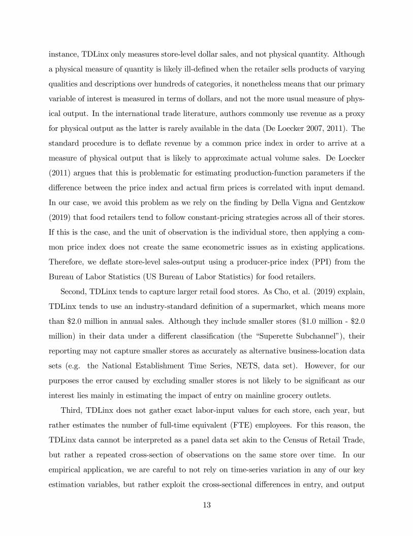
instance, TDLinx only measures store-level dollar sales, and not physical quantity. Although

a physical measure of quantity is likely ill-de�ned when the retailer sells products of varying

qualities and descriptions over hundreds of categories, it nonetheless means that our primary

variable of interest is measured in terms of dollars, and not the more usual measure of phys-

ical output. In the international trade literature, authors commonly use revenue as a proxy

for physical output as the latter is rarely available in the data (De Loecker 2007, 2011). The

standard procedure is to de�ate revenue by a common price index in order to arrive at a

measure of physical output that is likely to approximate actual volume sales. De Loecker

(2011) argues that this is problematic for estimating production-function parameters if the

di¤erence between the price index and actual �rm prices is correlated with input demand.

In our case, we avoid this problem as we rely on the �nding by Della Vigna and Gentzkow

(2019) that food retailers tend to follow constant-pricing strategies across all of their stores.

If this is the case, and the unit of observation is the individual store, then applying a com-

mon price index does not create the same econometric issues as in existing applications.

Therefore, we de�ate store-level sales-output using a producer-price index (PPI) from the

Bureau of Labor Statistics (US Bureau of Labor Statistics) for food retailers.

Second, TDLinx tends to capture larger retail food stores. As Cho, et al. (2019) explain,

TDLinx tends to use an industry-standard de�nition of a supermarket, which means more

than $2:0 million in annual sales. Although they include smaller stores ($1:0 million - $2:0

million) in their data under a di¤erent classi�cation (the �Superette Subchannel�), their

reporting may not capture smaller stores as accurately as alternative business-location data

sets (e.g. the National Establishment Time Series, NETS, data set). However, for our

purposes the error caused by excluding smaller stores is not likely to be signi�cant as our

interest lies mainly in estimating the impact of entry on mainline grocery outlets.

Third, TDLinx does not gather exact labor-input values for each store, each year, but

rather estimates the number of full-time equivalent (FTE) employees. For this reason, the

TDLinx data cannot be interpreted as a panel data set akin to the Census of Retail Trade,

but rather a repeated cross-section of observations on the same store over time. In our

empirical application, we are careful to not rely on time-series variation in any of our key

estimation variables, but rather exploit the cross-sectional di¤erences in entry, and output

13

values, to identify the impact of entry. Despite these potential shortcomings, we believe

the TDLinx data remains the best alternative for examining store-level markups using the

production-side approach of De Loecker and Warzynski (2012).

We summarize the key variables that enter our empirical model in Table 1 below. From

this table, it is clear that there is a substantial degree of variation in output and labor

input among stores, so the key parameters of interest should be identi�ed. In terms of

our entry-estimation objective, the data in this table also show considerable variation in

both the distance between each store and an entering hard-discounter, and the likelihood

of being proximate to an entering store. Therefore, we are con�dent that we have the

fundamental conditions in place to statistically identify the e¤ect of hard-discounter entry

on store performance.

[table 1 in here]

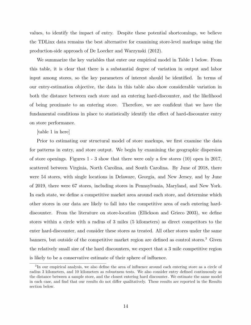
Prior to estimating our structural model of store markups, we �rst examine the data

for patterns in entry, and store output. We begin by examining the geographic dispersion

of store openings. Figures 1 - 3 show that there were only a few stores (10) open in 2017,

scattered between Virginia, North Carolina, and South Carolina. By June of 2018, there

were 54 stores, with single locations in Delaware, Georgia, and New Jersey, and by June

of 2019, there were 67 stores, including stores in Pennsylvania, Maryland, and New York.

In each state, we de�ne a competitive market area around each store, and determine which

other stores in our data are likely to fall into the competitive area of each entering hard-

discounter. From the literature on store-location (Ellickson and Grieco 2003), we de�ne

stores within a circle with a radius of 3 miles (5 kilometers) as direct competitors to the

enter hard-discounter, and consider these stores as treated. All other stores under the same

banners, but outside of the competitive market region are de�ned as control stores.3 Given

the relatively small size of the hard discounters, we expect that a 3 mile competitive region

is likely to be a conservative estimate of their sphere of in�uence.

3In our empirical analysis, we also de�ne the area of in�uence around each entering store as a circle ofradius 3 kilometers, and 10 kilometers as robustness tests. We also consider entry de�ned continuously asthe distance between a sample store, and the closest entering hard discounter. We estimate the same modelin each case, and �nd that our results do not di¤er qualitatively. These results are reported in the Resultssection below.

14

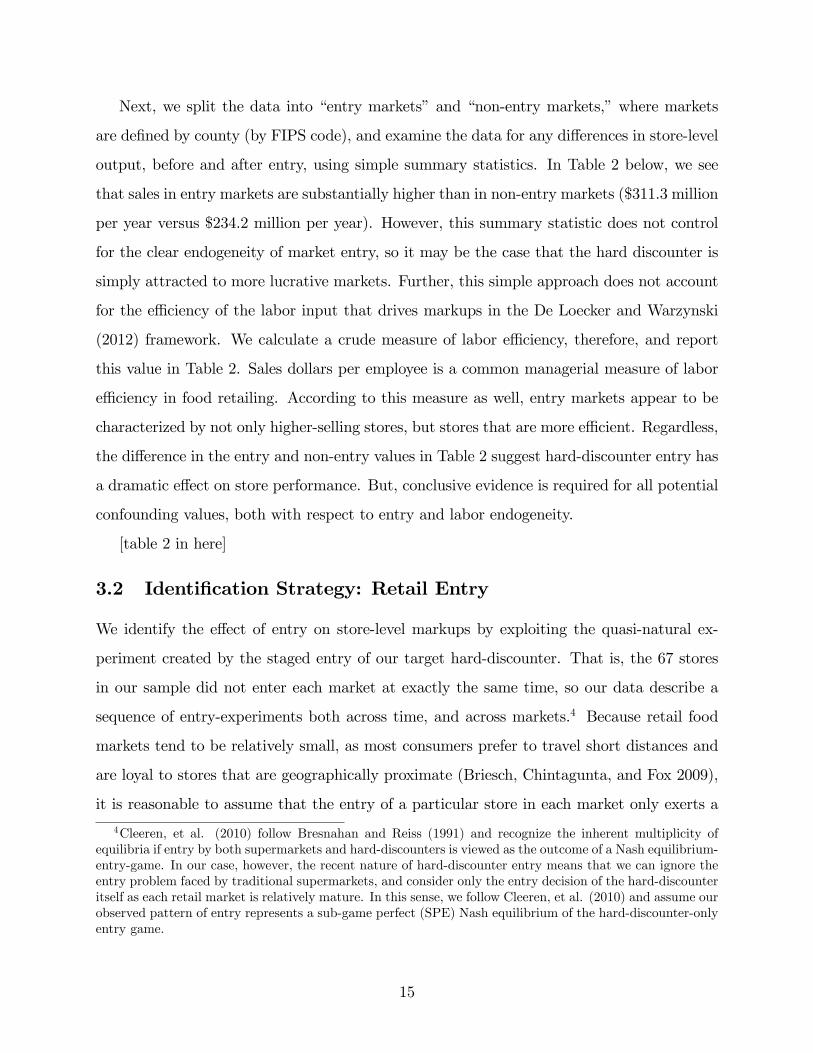
Next, we split the data into �entry markets�and �non-entry markets,�where markets

are de�ned by county (by FIPS code), and examine the data for any di¤erences in store-level

output, before and after entry, using simple summary statistics. In Table 2 below, we see

that sales in entry markets are substantially higher than in non-entry markets ($311.3 million

per year versus $234.2 million per year). However, this summary statistic does not control

for the clear endogeneity of market entry, so it may be the case that the hard discounter is

simply attracted to more lucrative markets. Further, this simple approach does not account

for the e¢ ciency of the labor input that drives markups in the De Loecker and Warzynski

(2012) framework. We calculate a crude measure of labor e¢ ciency, therefore, and report

this value in Table 2. Sales dollars per employee is a common managerial measure of labor

e¢ ciency in food retailing. According to this measure as well, entry markets appear to be

characterized by not only higher-selling stores, but stores that are more e¢ cient. Regardless,

the di¤erence in the entry and non-entry values in Table 2 suggest hard-discounter entry has

a dramatic e¤ect on store performance. But, conclusive evidence is required for all potential

confounding values, both with respect to entry and labor endogeneity.

[table 2 in here]

3.2 Identi�cation Strategy: Retail Entry

We identify the e¤ect of entry on store-level markups by exploiting the quasi-natural ex-

periment created by the staged entry of our target hard-discounter. That is, the 67 stores

in our sample did not enter each market at exactly the same time, so our data describe a

sequence of entry-experiments both across time, and across markets.4 Because retail food

markets tend to be relatively small, as most consumers prefer to travel short distances and

are loyal to stores that are geographically proximate (Briesch, Chintagunta, and Fox 2009),

it is reasonable to assume that the entry of a particular store in each market only exerts a

4Cleeren, et al. (2010) follow Bresnahan and Reiss (1991) and recognize the inherent multiplicity ofequilibria if entry by both supermarkets and hard-discounters is viewed as the outcome of a Nash equilibrium-entry-game. In our case, however, the recent nature of hard-discounter entry means that we can ignore theentry problem faced by traditional supermarkets, and consider only the entry decision of the hard-discounteritself as each retail market is relatively mature. In this sense, we follow Cleeren, et al. (2010) and assume ourobserved pattern of entry represents a sub-game perfect (SPE) Nash equilibrium of the hard-discounter-onlyentry game.

15

competitive in�uence on stores in that market. Entry into each market, however, is likely

to be endogenous to the expected pro�tability of the market (Cleeren et al. 2010). We ad-

dress this clear barrier to identi�cation using a set of instruments through a control-function

estimation framework.

First, we include a set of market-level �xed e¤ects that account for unobserved factors

that may be correlated with the decision to enter, an approach implemented by Klette

(1999) who used �xed e¤ects to capture di¤erences in levels of productivity due to variations

in labor quality. Fixed e¤ects are e¤ective instruments as they essentially absorb any local

conditions that are unobserved to the econometrician, and yet likely to be important to the

discounter�s decision to enter at that particular location. Thus, by including �xed e¤ects, we

allow cross-sectional di¤erences in productivity to be correlated with output and all factor

inputs (Klette 1999).

Second, we also include observed attributes of each local market (at the census-tract

level) from the American Community Survey (ACS, US Bureau of Census). ACS data are

useful in this regard as demographic and socioeconomic measures such as per capita income,

average household size, local unemployment, and residential rental rates are likely to be

highly correlated with purchasing-power measures considered by retailers in their decision

to enter a market, and yet mean independent of the productivity of each individual store.

Further, ACS provides exogenous variation at a level of geographic granularity that both

helps identify the entry-e¤ect we are interested in, and di¤erentiates local markets over time

and space.

Third, and perhaps most importantly, we use commercial real estate data (CRE, CoStar,

Inc.) for each entry-location. Our CRE data, de�ned as commercial sales prices per square

foot, represents an ideal instrument for the decision to enter as it re�ects market-level demand

for the speci�c location targeted by the entering store. Because we use market-level data

for a 3 km radius around the store, our sales prices are exogenous to the speci�c case of

the retailer, and are likely to capture a general level of demand for the location in question.

Retail lots used by grocery stores, moreover, are generally fungible across any retail purpose,

so CRE prices are independent of the output of a speci�c type of retailer. In our empirical

application, we examine the e¤ect of using each of these instruments on the robustness of

16

our empirical results, and determine their validity through �rst-stage instrumental variable

regressions. In a �rst-stage instrumental-variables regression of this set of instruments on

the decision to enter, estimated as a linear probability model, we �nd an F-statistic of 225.4,

so our instrument is not weak according to the threshold (F = 10:0) de�ned by Stock and

Yogo (2005). We report the complete results of these estimates in Table 3 below but, in

general, are con�dent that our identi�cation strategy supports our core hypotheses, and the

robustness of our empirical �ndings.

[table 3 in here]

Given that entry is a discrete variable, there is some debate over the exact form of the

control-variable model for the entry variable. While the traditional approach would apply

a Heckman-correction type of model with a suitable instrument, this approach is subject

to bias in the second stage if the �rst-stage probit model is mis-speci�ed. On the other

hand, Wooldridge (2015) argues that, in models such as this that are linear in the variables

with a discrete endogenous explanatory variable (EEV), it is preferred to estimate either a

�rst-stage probit equation, or a linear probability model, and use the generalized residuals

as control functions in the second-stage, structural model. When EEVs enter in non-linear

ways, as in our second-stage model, a control function method is preferred because �...for

general nonlinearities, inserting �tted values for EEVs is generally inconsistent, even under

strong assumptions (p. 429).� Therefore, we adopt a control function approach with the

generalized residuals from a �rst-stage, linear-probability model equation for the decision

to enter, instrumented with market �xed e¤ects, socioeconomic variables, and commercial

real-estate prices.

3.3 Identi�cation Strategy: Labor

As the literature on production-function estimation cited above clearly explains, the amount

of labor employed is also endogenous to any unobserved productivity shock at the store

level. In our static analog of the ACF (2015) approach, we instrument for the endogenous

labor input in the second-stage of the estimation procedure using a variable that is likely to

be highly correlated with the amount of store-level employment, but mean independent of

store output. According to �rst principles, �rms minimize cost by choosing the level of input

17

employment up to the point where the marginal value product is equal to the market wage. If

labor markets are competitive, the market wage should, therefore, be correlated with the level

of employment, but not necessarily related to the output level. Therefore, we use market-

level wages (de�ning each labor market at the county FIPS-code level) from the Quarterly

Census of Employment and Wages (QCEW, USBLS, 2020b) for workers in retail grocery

trade on a quarterly basis, and average over all quarters to arrive at an annual estimate of

the average weekly wage. For the labor input, our instrumental-variables regression of labor

employment on the average weekly wage and a constant produces an F-statistic of 391:5, so

again our instrument cannot be described as weak.

In the next section, we describe how these instruments help identify markups, and entry-

e¤ects using production-type data at the individual-store level.

4 Empirical Approach

We examine the problem of hard-discounter entry from both a reduced-form and structural

perspective. That is, we �rst examine the data using relatively simple, reduced-form models

to see if there are any patterns in the data that are consistent with our expectations regard-

ing the potential competitive e¤ects of hard-discounter entry on both volume and price of

incumbent retailers. We then estimate structural production functions that account for the

well-understood endogeneity of variable inputs (Olley and Pakes 1996; Levinsohn and Petrin

2003; Ackerberg, Caves, and Fraser 2015) using the approach developed for repeated-cross

sectional data by Lowrey, Richards, and Hamilton (2020). We use this approach to test

the e¤ect of entry on labor productivity, and markups, more formally. We then use the

estimates from this model to conduct a set of counterfactual simulations that compare prices

and markups with and without hard-discounter entry. We interpret the results from these

simulations as the likely welfare impacts of entry on �rms in our sample markets.5

5Note that we de�ne welfare e¤ects here from only the suppliers�perspective, as we do not estimate thestructural demand model that would be necessary to estimate consumer-welfare impacts. However, consumerwelfare is a¤ected by both variety and prices (Dixit and Stiglitz 1977), so the likely e¤ect on consumers isambiguous. While consumer welfare would rise due to lower prices, it would fall to the extent that there areany variety-reducing e¤ects attributable to the hard-discounter (Atkin et al. 2018). We leave the estimationnof these consumer-side e¤ects to future research.

18

4.1 Overview of Empirical Approach

In our �rst set of models, we examine price and volume data for any summary-level evidence

of hard-discounter entry. These models are not intended to be conclusive, but merely to

examine the data in a way that is relatively free from modeling constraints in order to see

if there are any patterns evident in the data. While the �ndings from these models may be

suggestive, there are not de�nitive tests of our core hypotheses regarding entry.

Our structural tests, on the other hand, address the endogeneity of input-choice and

entry using recently developed methods of markup estimation from the empirical trade and

industrial organization literatures (De Loecker and Warzynski 2012; De Loecker and Scott

2016). In a food-retail setting, we argue that a production-side approach to estimating the

extent of market power is preferred over the traditional, demand-side approach to margin

estimation (Villas-Boas 2007, for example) for several reasons.

First, the accuracy and consistency of markups estimated from a demand-side approach

depend on the relevance of the demand-model that is brought to the task. Although it

is well understood that random utility models applied to store level data are able to han-

dle multi-product, high-dimension problems that would otherwise overwhelm a traditional

demand-systems approach (Nevo 2001), they are not particularly well-suited to the scale of

demand problem presented by modern food retailers, where retailers typically sell 40,000 -

50,000 products in the same store, and consumers select items from among hundreds of prod-

uct categories. While others address the dimensionality problem inherent in retail demand

analysis using nested models of category-and-store choice (Bell and Lattin 1998; Richards,

Hamilton, and Yonezawa 2018), they are still only able to address the problem in an indirect

way, reducing the scale of the problem by ignoring most of it.

Second, retail demand estimation is also problematic because consumers�consideration

sets are unobserved, and endogenous (Mehta, Rajiv, and Srinivasan 2003; Koulayev 2014;

De Los Santos and Koulayev 2017). That is, traditional demand-side analysis assumes con-

sumers only shop from a limited set of products in any category that form the products

that they would reasonable consider buying. In actuality, however, the set of products

each consumer chooses from is endogenous to their preferences, experience, and the partic-

19

ular shopping environment, and analysts cannot measure (directly) the constituents of each

shopper�s consideration set. Koulayev (2014) shows that the resulting estimation bias can

be substantial.

Third, margin estimates derived from demand-elasticity estimates are conditional on a

speci�c solution concept that describes the game played among oligopolistic retailers. While

the literature appears to have settled on Bertrand-Nash rivalry as a reasonable and robust

way of thinking about how retailers interact, studies that adopt a �conduct parameter�

approach typically show substantial deviations from the maintained form of the pricing

game (Richards, Hamilton, and Yonezawa 2018).6 In contrast, the production-approach to

estimating markups makes no prior assumption on the nature of the game played among

competing �rms, and provides consistent estimates regardless of how retailers compete (De

Loecker 2011b).

Fourth, by de�nition, market entry presents unique problems for demand-side analyses

that are avoided by focusing only on store-level production. Speci�cally, if we seek to model

the structure of rivalry among competing retailers using changes in demand, and the cast

of players changes from one period to the next, then it is a di¢ cult task to disentangle the

e¤ects of changes in product-level interaction introduced by a new competitor from changes

in the game itself. By focusing only on the indirect impact of entry on each store�s input-

productivity, we obviate the need to take demand-reallocation into account.

Our point is that when we are interested in store-level outcomes, a production approach

has many appealing features relative to a more traditional demand-side approach. That said,

in our empirical model below, we describe how we need to modify, and thus depart from,

the approach developed by De Loecker and Warzynski (2012) to suit our particular needs.

4.2 Empirical Model

Researchers typically use panel data to estimate markups using the production-side approach

of De Loecker (2011a,b) and De Loecker and Warzynski 2012. There is nothing in the

underlying theory that requires panel data per se, but identifying the necessary productivity

6Corts (1999) criticizes the conduct parameter approach as being fundamentally unidenti�ed, and lackingin any meaningful theoretical basis in pricing behavior.

20

parameters generally requires methods developed speci�cally for application to panel data.

Speci�cally, the methods developed by Olley and Pakes (1996), Levinsohn and Petrin (2003),

and more recently by Ackerberg, Caves, and Fraser (ACF, 2015) all assume that productivity

shocks, which are correlated with endogenous input levels, follow Markov processes. In the

absence of panel data, researchers must therefore estimate input-productivity parameters

using cross-sectional data, as in our application, where the unobserved shocks to productivity

occur over �rms, and not over time. Therefore, the ACF approach is appropriate for data

that only describes variation in output across �rms, at the same point in time. Thus, our

empirical speci�cation of retail markups adopts the same conceptual framework to identifying

production-parameters as ACF (2015), but we depart from their approach, practically, due

to the particular application to food retail and our �rm-level data, which are repeated cross-

sections (described in detail in section 3.1).

Our empirical framework represents a contribution to the empirical industrial organiza-

tion literature on this subject, as we argue that there are many important problems that

simply cannot be addressed by either market-level demand data, nor by the type of census-

level data used by researchers in this area (Blonigen and Pierce 2016; De Loecker, Eeckhout,

and Unger 2020). Some of the most relevant research questions involve pro�tability and

productivity at the individual-establishment level that even �rm-level data (Traina 2018)

cannot appropriately address. For instance, the impact on consumer welfare of a proposed

merger is only relevant at the market level as consumers rarely travel more than a few miles

to an alternative real outlet, so �rm-level data would be useless for answering this ques-

tion. Retailing, particularly food retailing, is inherently local, so economic impact is only

relevant if measured at the level of the local market. Our approach is valuable, therefore,

as is provides consistent estimates of the necessary production parameters, as in Levinsohn

and Petrin (2003) or ACF (2015), but it may contain more practical relevance as it can

potentially meet with a far wider set of applications.

Our approach requires a consistent estimate of the output-elasticity with respect to one

variable input. In our case, the variable input of interest is labor, due both to its importance

to food retailers and its central role in empirical models of production more generally. Be-

cause most other retailing inputs either have a �xed relationship to output (e.g. materials,

21

or inventory) or are subject to substantial adjustment costs (e.g. capital, in the form of

the size of the store, or the technology used in the store) labor is an ideal input for our

purposes. It is well-understood, however, that labor employment is endogenous as shocks

that a¤ect output are also likely to a¤ect the �rm�s employment decisions (Olley and Pakes

1996; Levinsohn and Petrin 2003; Wooldridge 2009). Our two-step procedure, therefore, is

intended to address the fundamental endogeneity of labor-input, and the endogeneity of the

discounter�s decision to enter each particular market. We �rst invert the demand for an

input other than the variable input of interest, and use a non-parametric approach to obtain

a vector of expected production amounts that hold for any arbitrary parameterization of

the production surface. We then use the �tted values from this expression to remove any

observed shocks to productivity, and then use a control function approach to account for

the endogeneity of labor and the discrete decision to enter. It is in this second step that

we necessarily depart from ACF (2015) as our data are not dynamic, as required by their

Markov-productivity assumption.

4.2.1 Stage One: Estimating Retail Output

Our �rst-stage production function is a parametric model of output and two state, or quasi-

�xed, input variables. In the Olley and Pakes (1996) and Levinsohn and Petrin (2003)

framework, the demand for one state variable serves as a proxy variable for the unobserved

shock to productivity. In using this approach, we assume that productivity depends on

factors besides the variable input, and that values of these other factors are not determined

at the same time as employment decisions for the variable inputs are made. For our purposes,

we assume a relatively simple functional form for the production function (Cobb-Douglas),

in which output (yit) for store i in period t is a function of the amount of labor (lit) and two

quasi-�xed variables (e.g., the size of store i, k1it, and the number of checkouts, k2it), so the

production technology is given by:7

yit = �0 + �llit + �k1k1i + �k2k2i + �zzit + !it + �it; (4)

7Using a more complicated functional form would allow for greater �exibility in interacting among inputs,but we opt to achieve econometric �exibility by allowing the parameters of our Cobb-Douglas model to varyacross observations. We allow the marginal product of labor to vary over our sample, as in De Loecker andWarzynski (2012), but in a di¤erent, more parsimonious, way.

22

where each output and input value are expressed in logs, yit is de�ned as revenue at the store

level, normalized by a retail price index, labor lit is measured as the the number of employees

(full-time equivalent, FTE) in store i in year t, both k1i and k2i are time-invariant proxies

for di¤erent forms of capital investment, zit is a vector of exogenous explanatory variables

likely to be associated with inter-store di¤erences in productivity, the variable !it is a Hicks-

neutral productivity measure that cannot be observed by the analyst, and is assumed to be

correlated with lit, and �it is an i.i.d. error, which is assumed to be uncorrelated both over

�rms and time periods.8

With this approach, we require a variable that proxies the unobserved shock to produc-

tivity, and another that serves as a state variable. We de�ne k1i as the size of the store (in

square feet), and k2i as the number of checkouts, which we interpret as a measure of the

amount of investment in service technology deployed in the store. Although both measures

could plausibly serve in either role, we de�ne k1i as the proxy variable, as store size is more

likely to re�ect inter-store variation in productivity than any measure of technology usage,

and k2i as the state variable. In our data, we also have indicators of whether the store sells

gas or liquor, and the exact location of each store. We use these discrete measures on gas and

liquor sales as elements of the store-attribute (z) vector in the production-function above in

order to capture the e¤ect of observed store-heterogeneity on output, and labor productivity.

Our measures of store-location allow us to test the impact of an entering hard-discounter

on store productivity. We capture this e¤ect in two ways. First, we calculate the distance

between each store in our sample, and each hard-discounter. We then use this measure to

�nd the closest hard discounter, and de�ne a continuous variable, COMP , as a continuous

measure of the minimum distance between each store and the closest hard discounter. Sec-

ond, we use this distance calculation to express competitive pressure as a binary variable.

That is, we determine whether there is an outlet of the hard-discounter within 10, 5, or 3

kilometers (OPEN10, OPEN5, and OPEN3).9 Our hypothesis suggests that an entering

8De�ating store-level revenue by a retail-food price index to produce a physical measure of output islikely to induce measurement error in the dependent variable (De Loecker 2011b; De Loecker and Warzynski2012). However, we assume this error is subsumed in the general econometric error term and, as such, doesnot a¤ect the consistency of our estimates. Regardless, we de�ated store-revenue with a range of di¤erentretail-price indices, and our estimates were qualitatively similar under each approach.

9Our conversations with retail managers suggest that their locational-choice algorithm seeks to locate

23

hard discounter is likely to reduce incumbent-store markups, which requires that we interact

our competitive-pressure variables with the labor input in order to test the e¤ect of entry on

the marginal productivity of labor. We also include these competitive e¤ects as intercept-

shifting variables as entry is also likely to have a direct e¤ect on store sales, and not just

the e¢ ciency of a variable input. Because these measures are likely to be highly collinear,

we estimate di¤erent versions of the model, with each of these variables entering the model

separately. We report our �ndings as to the di¤erences in outcomes across these models in

the Results section below.

Our static version of the ACF (2015) approach retains their core assumptions: (i) the un-

observable is a scalar, and (ii) the proxy variable increases monotonically in the productivity

shock.10 Monotonicity is necessary so that we can write the unobserved shock to produc-

tivity as an arbitrary function of the state and proxy variables (k1i and k2i) and the vector

of store attributes. With these assumptions, therefore, we write the demand for retail �oor

space as:

k1i = h(k2i; !it; zit); (5)

where each element of the vector zit are potentially endogenous. The unobserved productivity

shock for i at time t is therefore written in terms of the inverse-demand for k1i, or:

!it = h�1(k1i; k2i; zit) = g(k1i; k2i; zit); (6)

where g(:) serves as an index of the productivity of �rm i.

In order to express the output of �rm i in terms of only observable and random factors,

we then follow the �rst-stage of the ACF (2015) procedure by substituting this expression

for the productivity shock back into the production function to arrive at:

yit = �0 + �llit + �k1k1i + �k2k2i + g(k1i; k2i; zit) + �it: (7)

stores such that there are no direct competitors within a 5 kilometer (3 mile) radius, so our competitivevariable is de�ned to capture a range around this measure. In this regard, our measure is very similar tothat used by Ellickson and Grieco (2013).10Monotonicity means that @k1i=@!it > 0, and De Loecker and Warzynski (2012) explain that this as-

sumption is true under any model of oligopolistic behavior, such as the Bertrand-Nash pricing assumptionthat is common in the retailing literature (Villas-Boas 2007). Mathematically, we require monotonicity inorder to invert the demand curve for the intermediate input.

24

Our �rst stage model consists of a non-parametric speci�cation of output as a arbitrary

function of proxy, capital and labor inputs: (lit; k1i; k2i; zit): There is some disagreement on

the nature of this speci�cation in the literature. While Olley and Pakes (1996) and Levinsohn

and Petrin (2003) argue that the marginal product of labor is identi�ed in (7), ACF (2015)

maintain instead that the labor parameter is not identi�ed as the amount of labor input is a

simple, deterministic function of the other arguments of the production function. We follow

ACF (2015) in this regard, as it is not necessary to use any estimates from the �rst-stage

model. Our non-parametric approach consists of a locally-weighted regression model with

arguments consisting of non-linear and interaction terms calculated from the values of labor,

capital, and proxy variables in the original production model (Levinsohn and Petrin 2003).

With this non-parametric model we obtain expected output values,^

; for any values of the

parameters in, �, and use these estimates to generate a control function, CFit; from the

residuals of the locally-weighted regression model.

4.2.2 Stage Two: Estimating Retail Productivity

Our departure from ACF (2015) occurs in the second-stage estimation model. Whereas their

underlying assumption maintains that the unobserved productivity shock follows a Markov

process, we do not have the sort of panel data that would allow us to exploit a similar

assumption. In their case, the Markov assumption means that the productivity shock can

be expressed as a stochastic function of lagged-values of productivity and an error term.

More generally, despite the number of applications of this model in the literature, we argue

that most production data sets are likely not up to this task, so are left in a similar position

as us. Instead, we assume that the productivity shocks represent idiosyncratic, store-level

di¤erences between stores in the same market. At the store level, di¤erences in productivity

between stores, most notably between stores in the same chain, are likely to re�ect di¤erences

in management style, employee training, or local demand conditions that re�ect deviations

from average-store productivity. Said di¤erently, the most important shock to productivity

is one that causes stores to di¤er from each other, and not from past versions of the same

store. In a mathematical sense, cross-sectional di¤erences in productivity are re�ected in the

control function estimated in the �rst-stage model, CFi, so the process underlying shocks to

25

productivity for �rm i are given by:

!it = CFi(_!t) + �it;

where_! re�ects industry-mean productivity.

In the second-stage model, therefore, we �rst subtract the CFit value from output, and

express the di¤erence as a linear (in logs) function of the proxy variable, capital, labor, store

attributes, and a new error term that re�ects di¤erences in productivity between store i and

the market-average:

yit � CFit = y�it = �0 + �llit + �k1k1i + �k2k2i + �zzit + �it + �it: (8)

In this model, however, labor is expected to be correlated with �it; so we estimate the second-

stage model using an instrumental variables approach. Further, in our model, recall that

there are also terms that re�ect discounter-entry in the z store-attribute vector. Regardless

of how these distance measures are calculated, each is endogenous to the discounter�s decision

to enter the market. Therefore, we include control functions for both the labor input and

the decision to enter. As we described above, the primary instrument for the labor input

consists of market-level wages for grocery store workers in the same county as the store in

question. From �rst principles, we know that wages are expected to be correlated with each

store�s demand for labor if managers minimize cost, but are mean-independent of store-level

output.11 We also include a set of store, year, and state �xed e¤ects as instruments.

Entry, however, presents a more di¢ cult identi�cation problem. An ideal instrument

would represent a measure of market-level demand for space, and hence represent the general

attractiveness of a particular location, and yet remain independent of any individual store�s

sales. For this purpose, therefore, we obtained ZIP-code level commercial real estate rental

rates for retail locations. Commercial real estate prices are exogenous to the performance of

any single �rm, and still re�ect the demand for each location for retail purposes. As we report

below, this instrument performs well in �rst-stage regressions on the discounter�s decisions

to enter each particular market. By adopting this control-function approach, we obtain

11In very-low income areas of the country, the average wage in a particular industry may re�ect aggregatepurchasing power, but given the general income-inelastic nature of food demand it is not likely to a¤ectstore-level sales.

26

consistent estimates of the output-elasticity of labor, the rest of the production-function

parameters, and the implied markups from the De Loecker and Warzynski (2012) approach.

Others in this literature estimate production functions that are more deeply parame-

terized than the Cobb-Douglas, for the simple purpose of obtaining labor-elasticity esti-

mates that vary over observations in the data set. Without further modi�cation, a Cobb-

Douglas production function implies an average value of the marginal product of labor (labor-

elasticity) that is expected to represent all of the �rms in the data. However, this assumption

is unsatisfactory as there is likely to be considerable heterogeneity remaining in the data,

even after accounting for the idiosyncratic productivity shocks above. Further, there are

more parsimonious ways of estimating models like this that still allow for parameters to

vary over cross-sectional observations in the data, without sacri�cing degrees of freedom, or

imposing additional structure on the model. Therefore, we account for unobserved hetero-

geneity in the data, and allow the marginal productivity of labor to vary across stores, but

estimating a random-parameter version of the second-stage production function model intro-

duced above. Each of the key production parameters is assumed to be normally distributed,

with parameter-heterogeneity also dependent upon the entry variables described above. In

this way, both the mean output levels for each store, and their markups, vary with the

discounter�s entry activity. We use this approach to test our core hypotheses, namely that

store-output, and markups, are both likely to be a¤ected by the entry of a hard-discounter.

5 Results

In this section, we �rst present results from a reduced-form estimation procedure, and then

the structural estimates of our markup-and-entry model. While the reduced-form model

results are suggestive of deeper patterns in the data, they are likely to be biased for the

reasons cited above.

Our reduced-form estimates control for state, chain, and year �xed e¤ects, as well as the

full set of production inputs and store-attribute values. These �ndings are in Table 4 below.

We estimate several versions of the model in order to examine the sensitivity of the core

model parameters, that is, the labor elasticity of output, to changing the set of covariates.

27

We estimate a basic model with only �xed e¤ects and production inputs (Model 1), a model

that includes store attributes (de�ned as whether the store sells gas or liquor, Model 2), a

model that adds the distance from an entering hard-discounter as an output-shifting variable

(Model 3), one that allows entry to a¤ect output and the labor-elasticity (Model 4), and a

model that de�nes entry as a discrete variable that takes a value of 1 if a hard-discounter

enters within 5 kilometers (Model 5). From the results in this table, we see that the core

output-elasticity estimates are relatively stable across the di¤erent speci�cations, and that

the implied returns to scale (the sum of the elasticities) is not statistically di¤erent from

1.0.12 Further, these reduced-form results show that output is greater for stores that sell

both gas and liquor, all else constant, so there are clear opportunities for cross-selling services

or alternative products in food retailing.

[table 4 in here]

Most important for our objectives, however, Model 3 shows that sales are signi�cantly

lower for stores nearer to an entering discounter than otherwise. But, controlling for the

dual e¤ects of entry on store output and labor e¢ ciency (Model 4), the results in this table

show that the main e¤ect of entry on output is felt through the e¢ ciency of labor, and not

gross output per se. In other words, each worker is able to generate less dollar sales than

without entry, which we interpret as implying that average prices are lower across the store

as management meets the new competitive pressure from the entering hard discounter. In

Model 4, however, the direct e¤ect of entry on store sales is not statistically signi�cant, while

it is in Model 5. We interpret the positive e¤ect of entry on store sales, controlling for the

e¤ect on labor productivity, as meaning that the entering hard-discounter drives incremental

tra¢ c to the area around the store, but forces prices down in equilibrium. Customers who

travel to the hard-discounter for low prices may not be able to �nd the products they want

in every category, however, in particular national brands (Hökelekli, Lamey, and Verboven

2017), so they shop at the nearest full-service supermarket in order to top o¤ their baskets.

After controlling for the endogeneity of entry and of labor inputs, we obtain structural

12This �nding is to be expected as competitive pressure and the relative maturity of retailers in our samplemean that they are not likely to either operate at levels that imply unexploited economies of scale (increasing)or well into the region of decreasing economies of scale.

28

estimates of labor-productivity on a store-level basis, and use these estimates to infer values

for the markup over marginal cost. These estimates are in Table 5 below. In this table,

we again report estimates from models that consider various de�nitions of entry, from the

distance to an entering hard-discounter (Model 1) to a binary indicator of a discounter within

3 kilometers (Model 2), 5 kilometers (Model 3), and 10 kilometers (Model 4). According to

the goodness-of-�t statistics reported in this table, it appears as though Model 4 provides

the best �t to the data among the �binary�models, although each �t the data slightly worse

than the continuous de�nition in Model 1. Because of the similarity in �t, and magnitude

of the estimated parameters, we interpret the parameters from Model 4, simply due to the

fact that we regard the binary de�nition of entry as the most consistent with how entry

likely impacts retailers�decisions in practice. That is, they are not likely to be a¤ected by a

discounter outside of what they regard as their market area, but will respond to what they

perceive as a direct competitor.

[table 5 in here]

Relative to the reduced-form estimates in Table 4, we see that controlling for both labor

and entry endogeneity leads to larger estimates for the output-elasticity with respect to labor.

According to the theoretical model of markup determination (Hall 1988), this implies higher

markups after controlling for endogeneity. In Model 4, the results also show a negative

marginal value of selling liquor, all else constant. Although liquor is notoriously a high-

volume, high-margin category, it may be the case that retailers have to employ additional

labor to manage the category, so controlling for labor-endogeneity removes any economic

bene�ts to selling liquor. Most importantly, however, the entry e¤ects from Table 4 are

con�rmed in this case. Namely, we �nd a similar pattern of entry-e¤ects on incumbent

retailers: Store output rises for stores that are near an entering hard-discounter (by an

average of 1:9%, using the data in Table 1), but margins fall. Relative to the reduced-form

evidence, our structural model shows an attenuated store-output e¤ect, but an accentuated

impact on labor-e¢ ciency. As in the previous table, we interpret this result as implying

that entering discounters drive tra¢ c to surrounding stores that provide more variety, but

increase pricing pressure on nearby retailers, reducing store-level markups.13

13We assume that hard-discounter entry has only a modest impact on retailing costs. This assumption

29

Our estimates represent non-trivial changes in pro�tability for stores exposed to hard-

discounter competition. In our preferred model (Model 4), the di¤erence in markups implied

by these estimates represents a 7:2% reduction in the price-cost margin. While this may

seem to be a small impact, retail food net margins, which also take into account �xed costs

of operation, tend to be roughly 2% (Campbell 2020). A 7% reduction in the amount of

margin available to pay �xed costs, therefore, can be substantial. For example, supposed a

2% margin represents a 50 pound bundle of groceries that sell for $2:00 per pound, with a

cost-of-goods-sold of $1:00 per pound, and a �xed cost of $48:00 for the store. Net pro�t

is $2:00 on sales of $100:00. If the price-cost markup falls from $1:00 to $0:93 per pound,

then this 2% net margin becomes a loss of 1:5%. Over the longer term, bankruptcy ensues,

regardless of the total sales e¤ect implied by our model.

Our �ndings are important to understanding both the broader, economic impacts of hard-

discounter entry, and potential managerial responses. First, although we do not calculate

the implied welfare e¤ects on competing �rms and consumers that buy from these retailers,

it is clear from our results that producer surplus is likely to fall due to lower markups, but

consumer surplus will rise for the same reason. To the extent that incumbent retailers may

also reduce their SKU count in order to compete with hard discounters, consumers may also

experience a reduction in welfare from a loss of variety. In general, however, lower prices tend

to be net positive for consumers. Second, retail managers need to be aware of the potential

consequences due to the entry of paradigm-changing retailers like hard-discounters, and draft

responses that are least likely to be self-destructive. For instance, Arcidiacono et al. (2016)

describe the impact on local markets due to Walmart�s entry into retail markets throughout

the 1990s and 2000s. While the common perception was that �main street�would su¤er

most, it was instead the direct competitors to Walmart �the supermarkets that competed

most directly with Walmart�s primary line of business. In fact, retailers that were su¢ ciently

di¤erentiated from Walmart were less a¤ected, if at all. Our �ndings make a similar case,

namely that responding by reducing prices and SKUs in order to match the hard-discounters�

business models will likely end in failure, but di¤erentiating by emphasizing variety, quality,

is reasonable because even Walmart carrying a larger assortment of national brand products has a minimalimpacts at the wholesale market level (Huang et al. 2012).

30

and sharply di¤erentiated store brands (Hökelekli, Lamey, and Verboven 2017) is more likely

to be successful.

6 Conclusions and Implications

In this paper, we examine the impact of hard-discounter entry on incumbent retailer markups.

Because retailers tend to sell thousands of items, we argue that the traditional demand-side

approach to entry is intractable for a problem like this, so adopt the production-side markup-

estimation approach of De Loecker and Warzynski (2012) for this purpose. Although this

approach has been used extensively to estimate the e¤ect of trade status on manufacturing

margins (De Loecker 2007) or corporate markups in general (De Loecker, Eeckhout, and

Unger 2020), we are the �rst to use this approach to examine retail-store performance.

We �nd that, averaged over all incumbent retailers and markets, markups fall by over

7:0% in response to hard-discounter entry, although total store sales rise by nearly 2:0%.

There are two mechanisms that explain these e¤ects: First, competitive pressure from enter-

ing hard-discounters causes retail prices, and hence markups, to fall and, second, customers

shop in nearby stores in order to �ll their baskets with items that are not available at the

hard-discounter. This �nding is remarkably consistent with others who document this same

inter-store complementarity e¤ect using entirely di¤erent methods and data (Vroegrijk, Gi-

jsbrechts, and Campo 2013). Higher sales, however, are likely irrelevant if the lower markup

causes already-low-margin retailers to sell at a loss.

Our empirical model has both macroeconomic and managerial signi�cance. If the spread

of hard-discounters leads to lower retail prices for food, then consumers will almost certainly

bene�t in terms of total welfare. However, if hard-discounter entry leads to the exit of grocery

stores in nearby markets, that were perhaps already marginally suited to traditional grocery

retailers, then the �food desert�problem may be accentuated in these markets (Allcott, et

al. 2019). Finding that store sales rise in response to new entry suggests a way out of the

implied competitive trap for existing retailers � rather than respond to entering retailers

by restructuring in order to �beat them at their own game,� our �ndings suggest instead

that retailers are better o¤pivoting away from these new formats, o¤ering instead what hard

31

discounters do not. For example, this means o¤ering a greater variety of national brands, and

perhaps store brands that o¤er more favorable price-quality perceptions than those o¤ered

by the hard discounters (Cleeren, et al. 2010; Lourenco and Gijsbrechts 2013).

Our research has some limitations. First, the TDLinx data that forms the core of our

empirical model only includes estimates of the output for each sample store. However,

Nielsen, the provider of TDLinx, has a commercial stake in ensuring the quality and accuracy

of these estimates, so are data are likely as good as any available alternative. Second, we

estimate a relatively simple production surface for our sample retailers. While others in

this literature estimate translog models in order to capture interactions between inputs,

and other sources of non-linearity, we take a more parsimonious approach, and introduce

�exibility through the use of a random-parameter production speci�cation. To the extent

that our approach does not capture the same underlying structure, our estimates will be in

err. Third, the retailer that forms the focus of our paper entered only a limited number of

markets (10 states) over a 3-year period. A longer time-series of entry events would have

likely provided sharper identi�cation conditions for our core model. That said, the e¤ects

we describe appear to be precisely estimated, so it may be the case that more data were not

needed.

32

References

[1] Ackerberg, D. A., Caves, K., & Frazer, G. (2015). Identi�cation properties of recent

production function estimators. Econometrica, 83(6), 2411-2451.

[2] Ailawadi, K. L., Zhang, J., Krishna, A., & Kruger, M. W. (2010). When Wal-Mart

enters: How incumbent retailers react and how this a¤ects their sales outcomes. Journal

of Marketing Research, 47(4), 577-593.

[3] Allcott, H., Diamond, R., Dubé, J. P., Handbury, J., Rahkovsky, I., & Schnell, M.

(2019). Food deserts and the causes of nutritional inequality. Quarterly Journal of Eco-

nomics, 134(4), 1793-1844.

[4] Arcidiacono, P., Bayer, P., Blevins, J. R., & Ellickson, P. B. (2016). Estimation of

dynamic discrete choice models in continuous time with an application to retail compe-

tition. Review of Economic Studies, 83(3), 889-931.

[5] Asker, J., Collard-Wexler, A., & De Loecker, J. (2014). Dynamic inputs and resource

(mis) allocation. Journal of Political Economy, 122(5), 1013-1063.

[6] Atkin, D., Faber, B. & Gonzalez-Navarro, M. (2018). Retail globalization and household

welfare: Evidence from Mexico. Journal of Political Economy, 126(1): 1-73.

[7] Bauner, C., & Wang, E. (2019). The e¤ect of competition on pricing and product

positioning: Evidence from wholesale club entry. International Journal of Industrial

Organization, 67, 102525.

[8] Basker, E. (2005). Selling a cheaper mousetrap: Wal-Mart�s e¤ect on retail prices.

Journal of Urban Economics, 58(2), 203-229.

[9] Basker, E., & Noel, M. (2009). The evolving food chain: competitive e¤ects of Wal-

Mart�s entry into the supermarket industry. Journal of Economics & Management Strat-

egy, 18(4), 977-1009.

[10] Basker, E. (2012). Raising the barcode scanner: Technology and productivity in the

retail sector. American Economic Journal: Applied Economics, 4(3), 1-27.

33

[11] Basu, S. (2019). Are price-cost markups rising in the United States? a discussion of the

evidence. Journal of Economic Perspectives, 33(3), 3-22.

[12] Begley, S., Hancock, B., Kilroy, T., & Kohli, S. (2019, May 23). Automation

in retail: An executive overview for getting ready. McKinsey & Company Re-

tail Insights. (https://www.mckinsey.com/industries/retail/our-insights/automation-

in-retail-an-executive-overview-for-getting-ready). Accessed February 23, 2021.

[13] Bell, D. R., & Lattin, J. M. (1998). Shopping behavior and consumer preference for store

price format: Why �large basket�shoppers prefer EDLP. Marketing Science, 17(1), 66-

88.

[14] Beresteanu, A., Ellickson, P., & Misra, S. (2010). The dynamics of retail oligopoly.

Department of Economics, University of Pittsburgh. Working paper.

[15] Blonigen, B. A., & Pierce, J. R. (2016). Evidence for the e¤ects of mergers on market

power and e¢ ciency (No. w22750). National Bureau of Economic Research.

[16] Borraz, F., Dubra, J., Ferrés, D., & Zipitría, L. (2014). Supermarket entry and the

survival of small stores. Review of Industrial Organization, 44(1), 73-93.

[17] Bresnahan, T. F., & Reiss, P. C. (1991). Entry and competition in concentrated markets.

Journal of Political Economy, 99(5), 977-1009.

[18] Briesch, R. A., Chintagunta, P. K., & Fox, E. J. (2009). How does assortment a¤ect

grocery store choice? Journal of Marketing Research, 46(2), 176-189.

[19] Bronnenberg, B. J., & Ellickson, P. B. (2015). Adolescence and the path to maturity in

global retail. Journal of Economic Perspectives, 29(4), 113-34.

[20] Campbell, J. (2020). What is the pro�t margin for grocery stores?

(https://thegrocerystoreguy.com). Accessed Oct. 28, 2020.

[21] Cho, C., McLaughlin, P. W., Zeballos, E., Kent, J., and Dicken, C. (2019). Capturing the

complete food environment with commercial data: A comparison of TDLinx, ReCount,

and NETS databases. Economic Research Service, USDA. Technical Bulletin No. 1953.

34

[22] Cleeren, K., Verboven, F., Dekimpe, M. G., & Gielens, K. (2010). Intra-and interformat

competition among discounters and supermarkets. Marketing Science, 29(3), 456-473.

[23] Corts, K. S. (1999). Conduct parameters and the measurement of market power. Journal

of Econometrics, 88(2), 227-250.

[24] Courtemanche, C., & Carden, A. (2011). Supersizing supercenters? The impact of

Walmart Supercenters on body mass index and obesity. Journal of Urban Economics,

69(2), 165-181.

[25] Courtemanche, C., & Carden, A. (2014). Competing with Costco and Sam�s Club:

Warehouse club entry and grocery prices. Southern Economic Journal, 80(3), 565-585.

[26] De Loecker, J. (2007). Do exports generate higher productivity? Evidence from Slovenia.

Journal of International Economics, 73(1), 69-98.

[27] De Loecker, J. (2011a). Product di¤erentiation, multiproduct �rms, and estimating the

impact of trade liberalization on productivity. Econometrica, 79(5), 1407-1451.

[28] De Loecker, J. (2011b). Recovering markups from production data. International Jour-

nal of Industrial Organization, 29(3), 350-355.

[29] De Loecker, J., &Warzynski, F. (2012). Markups and �rm-level export status. American

Economic Review, 102(6), 2437-71.

[30] De Loecker, J., & Scott, P. T. (2016). Estimating market power: Evidence from the US

brewing industry. Working paper no. w22957. National Bureau of Economic Research.

[31] De Loecker, J., Eeckhout, J., & Unger, G. (2020). The rise of market power and the

macroeconomic implications. Quarterly Journal of Economics, 135(2), 561-644.

[32] De los Santos, B., & Koulayev, S. (2017). Optimizing click-through in online rankings

with endogenous search re�nement. Marketing Science, 36(4), 542-564.

[33] DellaVigna, S., & Gentzkow, M. (2019). Uniform pricing in us retail chains. Quarterly

Journal of Economics, 134(4), 2011-2084.

35

[34] Dickson, P. R., & Sawyer, A. G. (1990). The price knowledge and search of supermarket

shoppers. Journal of Marketing, 54(3), 42-53.

[35] Ellickson, P. B. (2016). The evolution of the supermarket industry: from A & P to

Walmart. Handbook on the Economics of Retailing and Distribution, Edward Elgar

Publishing.

[36] Ellickson, P. B., & Grieco, P. L. (2013). Wal-Mart and the geography of grocery retailing.

Journal of Urban Economics, 75, 1-14.

[37] FMI. (2021). Supermarket facts. (https://www.fmi.org/our-research/supermarket-

facts). Accessed February 23, 2021.

[38] Foster, L., Haltiwanger, J., & Krizan, C. J. (2006). Market selection, reallocation, and

restructuring in the US retail trade sector in the 1990s. Review of Economics and Sta-

tistics, 88(4), 748-758.

[39] Foster, L., Haltiwanger, J., & Syverson, C. (2008). Reallocation, �rm turnover, and

e¢ ciency: Selection on productivity or pro�tability? American Economic Review, 98(1),

394-425.

[40] Gelper, S., Wilms, I., & Croux, C. (2016). Identifying demand e¤ects in a large network

of product categories. Journal of Retailing, 92(1), 25-39.

[41] Hall, R. E. (1988). The relation between price and marginal cost in US industry. Journal

of Political Economy, 96(5), 921-947.

[42] Hall, R. E. (2018). New evidence on the markup of prices over marginal costs and

the role of mega-�rms in the us economy (No. w24574). National Bureau of Economic

Research.

[43] Hausman, J., & Leibtag, E. (2007). Consumer bene�ts from increased competition in

shopping outlets: Measuring the e¤ect of Wal-Mart. Journal of Applied Econometrics,

22(7), 1157-1177.

36

[44] Hökelekli, G., Lamey, L., & Verboven, F. (2017). The battle of traditional retailers

versus discounters: The role of PL tiers. Journal of Retailing and Consumer Services,

39, 11-22.

[45] Holmes, T. J. (2011). The di¤usion of Wal-Mart and economies of density. Econometrica,

79(1), 253-302.

[46] Huang, Q., Nijs, V. R., Hansen, K., & Anderson, E. T. (2012). Wal-Mart�s impact on

supplier pro�ts. Journal of Marketing Research, 49(2), 131-143.

[47] Iacovone, L., Javorcik, B., Keller, W., & Tybout, J. (2015). Supplier responses to Wal-

mart�s invasion in Mexico. Journal of International Economics, 95(1), 1-15.

[48] Inman, J. J., & Nikolova, H. (2017). Shopper-facing retail technology: A retailer adop-

tion decision framework incorporating shopper attitudes and privacy concerns. Journal

of Retailing, 93(1), 7-28.

[49] Jackson, K. (2020). What is Lidl? Why this discount grocery store is giving Aldi a run for

its money. (https://www.today.com/food/what-lidl-discount-grocery-store-giving-aldi-

run-its-money-t182688). Accessed September 24, 2020.

[50] Jia, P. (2008). What happens when Wal-Mart comes to town: An empirical analysis of

the discount retailing industry. Econometrica, 76(6), 1263-1316.

[51] Klette, T. J. (1999). Market power, scale economies and productivity: estimates from

a panel of establishment data. The Journal of Industrial Economics, 47(4), 451-476.

[52] Koulayev, S. (2014). Search for di¤erentiated products: identi�cation and estimation.

RAND Journal of Economics, 45(3), 553-575.

[53] Lagakos, D. (2016). Explaining cross-country productivity di¤erences in retail trade.

Journal of Political Economy, 124(2), 579-620.

[54] Levinsohn, J., & Petrin, A. (2003). Estimating production functions using inputs to

control for unobservables. Review of Economic Studies, 70(2), 317-341.

37

[55] Lit�n, T., & Wolfram, G. (2006). New automated checkout systems. in Retailing in

the 21st Century, Kra¤t Manfred and Mantrala Murali K., eds. Berlin/Heidelberg/New

York: Springer.

[56] Lourenço, C. J., & Gijsbrechts, E. (2013). The impact of national brand introduc-

tions on hard-discounter image and share-of-wallet. International Journal of Research

in Marketing, 30(4), 368-382.

[57] Lowrey, J., Richards, T. J. & S. F. Hamilton. (2020). Food banks and retail markups.

Working paper, Fisher College of Business, Ohio State University, Columbus, OH.

[58] Loy, J. P., Ceynowa, C., & Kuhn, L. (2020). Price recall: Brand and store type di¤er-

ences. Journal of Retailing and Consumer Services, 53, 1-13.

[59] Mehta, N., Rajiv, S., & Srinivasan, K. (2003). Price uncertainty and consumer search:

A structural model of consideration set formation. Marketing Science, 22(1), 58-84.

[60] Nevo, A. (2001). Measuring market power in the ready-to-eat cereal industry. Econo-

metrica, 69(2), 307-342.

[61] Progressive Grocer. (2019). Grocerys must not ignore the hard-discounter threat: Re-

port. (https://progressivegrocer.com/grocers-must-not-ignore-hard-discounter-threat-

report). Accessed Nov. 17, 2020.

[62] Progressive Grocer. (2020). 5 Critical pricing lessons from the COVID-19

pandemic. (https://www.demandtec.com/resources/5-critical-pricing-lessons-from-the-

covid-19-pandemic/). Accessed Nov. 5, 2020.

[63] Richards, T. J., Hamilton, S. F., & Yonezawa, K. (2018). Retail market power in a

shopping basket model of supermarket competition. Journal of Retailing, 94(3), 328-

342.

[64] Singh, V. P., Hansen, K. T., & Blattberg, R. C. (2006). Market entry and consumer

behavior: An investigation of a Wal-Mart supercenter. Marketing Science, 25(5), 457-

476.

38

[65] Solow, R. M. (1957). Technical change and the aggregate production function. Review

of Economics and Statistics, 312-320.

[66] Steenkamp, J. B. E. (2018). Brands and retailers under attack from hard discounters,

in Handbook of Research on Retailing. pp. 44-64. Northhampton, MA: Edward Elgar

Publishing.

[67] Stock, J. H., & Yogo, M. (2005). Testing for weak instruments in linear IV regres-

sion. Identi�cation and Inference for Econometric Models: Essays in Honor of Thomas

Rothenberg, 80.

[68] Syverson, C. (2019). Macroeconomics and market power: Context, implications, and

open questions. Journal of Economic Perspectives, 33(3), 23-43.

[69] Thomassen, Ø., Smith, H., Seiler, S., & Schiraldi, P. (2017). Multi-category competition

and market power: a model of supermarket pricing. American Economic Review, 107(8),

2308-51.

[70] Traina, J. (2018). Is aggregate market power increasing? production trends using �-

nancial statements. Production Trends Using Financial Statements (February 8, 2018).

University of Chicago, Working paper.

[71] Turner, N., Wang, S., & Soper, S. (2017). Amazon to Acquire Whole Foods for $13.7 Bil-

lion. Bloomberg Technology. (https://www.bloomberg.com/news/articles/2017-06-16).

Accessed on September 29, 2020.

[72] United States Bureau of Labor Statistics. (2020a). Prices - Producer.

(https://www.bls.gov/data/). Accessed September 15, 2020.

[73] United States Bureau of Labor Statistics. (2020b). Quarterly Census of Employment

and Wages. (https://www.bls.gov/cew/). Accessed September 19, 2020.

[74] United States Bureau of Census. American Community Survey.

(https://www.census.gov/programs-surveys/acs/data.html). Accessed September

20, 2020.

39

[75] Villas-Boas, S. B. (2007). Vertical relationships between manufacturers and retailers:

Inference with limited data. Review of Economic Studies, 74(2), 625-652.

[76] Vroegrijk, M., Gijsbrechts, E., & Campo, K. (2013). Close encounter with the hard

discounter: A multiple-store shopping perspective on the impact of local hard-discounter

entry. Journal of Marketing Research, 50(5), 606-626.

[77] Vroegrijk, M., Gijsbrechts, E., & Campo, K. (2016). Battling for the household�s cate-

gory buck: Can economy private labels defend supermarkets against the hard-discounter

threat? Journal of Retailing, 92(3), 300-318.

[78] Wooldridge, J. M. (2009). On estimating �rm-level production functions using proxy

variables to control for unobservables. Economics Letters, 104(3), 112-114.

[79] Wooldridge, J. M. (2015). Control function methods in applied econometrics. Journal

of Human Resources, 50(2), 420-445.

[80] Zhu, T., & Singh, V. (2009). Spatial competition with endogenous location choices: An

application to discount retailing. Quantitative Marketing and Economics, 7(1), 1-35.

40

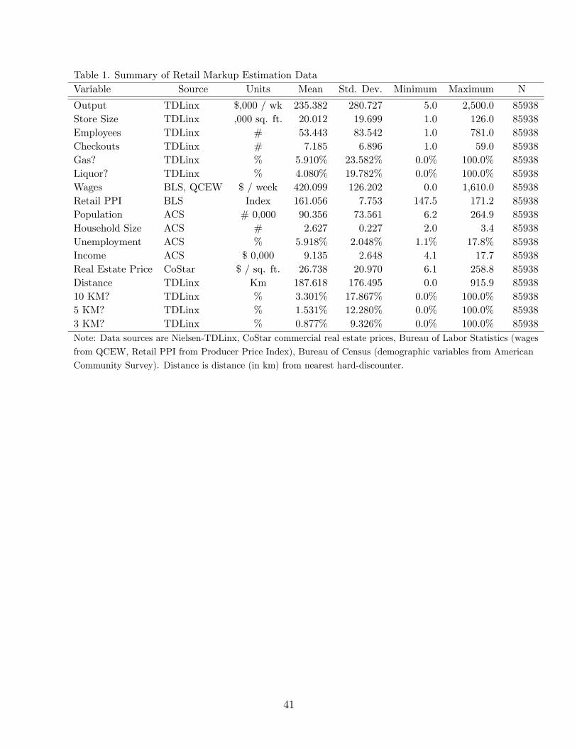
Table 1. Summary of Retail Markup Estimation DataVariable Source Units Mean Std. Dev. Minimum Maximum N

Output TDLinx $,000 / wk 235.382 280.727 5.0 2,500.0 85938Store Size TDLinx ,000 sq. ft. 20.012 19.699 1.0 126.0 85938Employees TDLinx # 53.443 83.542 1.0 781.0 85938Checkouts TDLinx # 7.185 6.896 1.0 59.0 85938Gas? TDLinx % 5.910% 23.582% 0.0% 100.0% 85938Liquor? TDLinx % 4.080% 19.782% 0.0% 100.0% 85938Wages BLS, QCEW $ / week 420.099 126.202 0.0 1,610.0 85938Retail PPI BLS Index 161.056 7.753 147.5 171.2 85938Population ACS # 0,000 90.356 73.561 6.2 264.9 85938Household Size ACS # 2.627 0.227 2.0 3.4 85938Unemployment ACS % 5.918% 2.048% 1.1% 17.8% 85938Income ACS $ 0,000 9.135 2.648 4.1 17.7 85938Real Estate Price CoStar $ / sq. ft. 26.738 20.970 6.1 258.8 85938Distance TDLinx Km 187.618 176.495 0.0 915.9 8593810 KM? TDLinx % 3.301% 17.867% 0.0% 100.0% 859385 KM? TDLinx % 1.531% 12.280% 0.0% 100.0% 859383 KM? TDLinx % 0.877% 9.326% 0.0% 100.0% 85938Note: Data sources are Nielsen-TDLinx, CoStar commercial real estate prices, Bureau of Labor Statistics (wages

from QCEW, Retail PPI from Producer Price Index), Bureau of Census (demographic variables from American

Community Survey). Distance is distance (in km) from nearest hard-discounter.

41

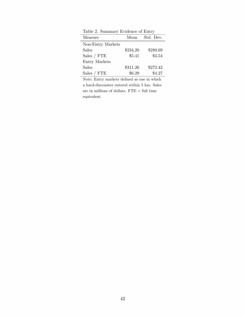
Table 2. Summary Evidence of EntryMeasure Mean Std. Dev.

Non-Entry MarketsSales $234.20 $280.69Sales / FTE $5.41 $3.54Entry MarketsSales $311.26 $272.42Sales / FTE $6.29 $4.27Note: Entry markets de�ned as one in which

a hard-discounter entered within 5 km. Sales

are in millions of dollars. FTE = full time

equivalent.

42

Table 3. IV Estimates for Labor and Entry VariablesEntry Model Labor Input Model

Estimate Std. Err. Estimate Std. Err.

Constant 0.0688 0.0063 6.0935 0.1434State 1 -0.0487 0.0047State 2 -0.0572 0.0019State 3 -0.0571 0.0022State 4 -0.0510 0.0020State 5 -0.0562 0.0017State 6 -0.0258 0.0018State 7 -0.0573 0.0018State 8 -0.0178 0.0023Population -0.0092 0.0008Household Size 0.0132 0.0021Unemployment -0.3761 0.0266Income -0.0022 0.0002CRE Rent 0.0003 0.0000Ave. Wage -0.4664 0.0236F 225.4210 391.4771R2 0.0330 0.0045Note: Demographic data from American Community Survey, CRE

(commercial real estate) rent from CoStar, and wages are from QCEW

(US Bureau of Labor Statistics). A single asterisk indicates signif-

icance at a 5% level.

43

Table4.Reduced-FormProductionFunctionEstimates

Model1

Model2

Model3

Model4

Model5

Variables

Mean

Std.Err.

Mean

Std.Err.

Mean

Std.Err.

Mean

Std.Err.

Mean

Std.Err.

Labor

0.6004

0.0019

0.5995

0.0019

0.5993

0.0019

0.6120

0.0047

0.5997

0.0019

Capital1

0.1637

0.0019

0.1630

0.0019

0.1633

0.0019

0.1631

0.0019

0.1629

0.0019

Capital2

0.1941

0.0029

0.1950

0.0029

0.1948

0.0029

0.1948

0.0029

0.1950

0.0029

Gas

0.0673

0.0049

0.0675

0.0049

0.0669

0.0049

0.0675

0.0049

Liquor

0.0192

0.0061

0.0208

0.0062

0.0221

0.0062

0.0203

0.0061

Entry

-0.0038

0.0015

0.0037

0.0030

0.1242

0.0357

Entry*Labor

-0.0022

0.0007

-0.0217

0.0096

ChainE¤ects

Yes

Yes

Yes

Yes

Yes

YearE¤ects

Yes

Yes

Yes

Yes

Yes

StateE¤ects

Yes

Yes

Yes

Yes

Yes

RandomParameters

Yes

Yes

Yes

Yes

Yes

AIC/N

0.752

0.751

0.751

0.751

0.750

LLF

-3.154

-3.207

-3.208

-3.207

-3.207

Note:Allcovariatesareinnaturallogs.Model1isthecoreCobb-Douglasproductionfunctionwithrandom-

parameters,andnoothervariables.Model2isModel1withstoreattributes.Model3includesentryde�ned

asdistancetohard-discountera¤ectingmeansales.Model4isModel3withlaborandentryinteracted,while

Model5includesentryde�nedasdiscreteindicatorfornewdiscounterwithin5km.AICistheAkaikeInformation

Criterion.Note:Dataforallmodelsfrom

NielsenTDLinx,BLS-QCEW,bystore.Forallmodels,N=85,938.

44

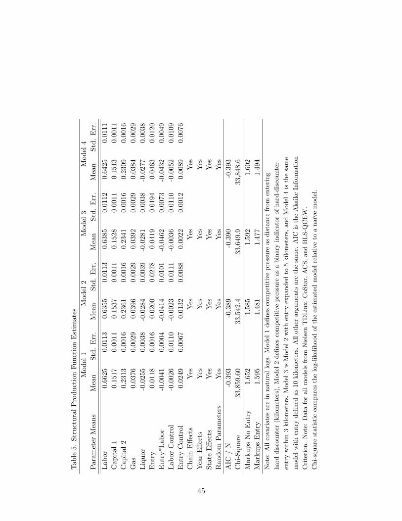
Table5.StructuralProductionFunctionEstimates

Model1

Model2

Model3

Model4

ParameterMeans

Mean

Std.Err.

Mean

Std.Err.

Mean

Std.Err.

Mean

Std.Err.

Labor

0.6625

0.0113

0.6355

0.0113

0.6385

0.0112

0.6425

0.0111

Capital1

0.1517

0.0011

0.1537

0.0011

0.1528

0.0011

0.1513

0.0011

Capital2

0.2313

0.0016

0.2361

0.0016

0.2341

0.0016

0.2309

0.0016

Gas

0.0376

0.0029

0.0396

0.0029

0.0392

0.0029

0.0384

0.0029

Liquor

-0.0255

0.0038

-0.0284

0.0039

-0.0281

0.0038

-0.0277

0.0038

Entry

0.0118

0.0016

0.0200

0.0278

0.0419

0.0194

0.0463

0.0120

Entry*Labor

-0.0041

0.0004

-0.0414

0.0101

-0.0462

0.0073

-0.0432

0.0049

LaborControl

-0.0026

0.0110

-0.0023

0.0111

-0.0036

0.0110

-0.0052

0.0109

EntryControl

0.0249

0.0067

0.0132

0.0088

0.0022

0.0012

0.0089

0.0076

ChainE¤ects

Yes

Yes

Yes

Yes

YearE¤ects

Yes

Yes

Yes

Yes

StateE¤ects

Yes

Yes

Yes

Yes

RandomParameters

Yes

Yes

Yes

Yes

AIC/N

-0.393

-0.389

-0.390

-0.393

Chi-Square

33,859.60

33,542.4

33,649.9

33,848.6

MarkupsNoEntry

1.652

1.585

1.592

1.602

MarkupsEntry

1.595

1.481

1.477

1.494

Note:Allcovariatesareinnaturallogs.Model1de�nescompetitivepressureasdistancefrom

entering

harddiscounter(kilometers),Model2de�nescompetitivepressureasabinaryindicatorofhard-discounter

entrywithin3kilometers,Model3isModel2withentryexpandedto5kilometers,andModel4isthesame

modelwithentryde�nedas10kilometers.Allotherargumentsarethesame.AICistheAkaikeInformation

Criterion.Note:Dataforallmodelsfrom

NielsenTDLinx,CoStar,ACS,andBLS-QCEW.

Chi-squarestatisticcomparesthelog-likelihoodoftheestimatedmodelrelativetoanaïvemodel.

45