resource assessment on the economic viability of … assessment on the economic viability of the...
TRANSCRIPT

100 SUMMER STREET, SUITE 3200BOSTON, MASSACHUSETTS 02110
TEL 617-531-2818FAX 617-531-2826
Resource Assessment on the Economic Viability of the Millstone Nuclear Generating Facilities
prepared for
Connecticut Department of Energy & Environmental Protection
Connecticut Public Utilities Regulatory Authority
December 7, 2017

TABLE OF CONTENTS
Executive Summary .................................................................................................................... ES-1
Millstone Cash Flows ............................................................................................................. ES-1
Millstone Replacement Costs ................................................................................................ ES-4 0% Replacement Case ........................................................................................................ ES-5 25% Replacement Case ...................................................................................................... ES-6 100% Replacement Case .................................................................................................... ES-7 Comparison of Results ....................................................................................................... ES-8
Economic Impact Analysis.................................................................................................... ES-10
1 Wholesale Electricity Market in New England ........................................................................ 1
1.1 Energy Forecast ................................................................................................................ 2 1.1.1 Reference Case Assumptions (With Millstone) ........................................................ 3 1.1.2 Sensitivities ............................................................................................................. 19 1.1.3 Retirement Analysis ................................................................................................ 29 1.1.4 Results ..................................................................................................................... 33
1.2 Capacity Price Forecast .................................................................................................. 49 1.2.1 Millstone Historical FCA Revenues ......................................................................... 49 1.2.2 Forward Capacity Market Structure ....................................................................... 50 1.2.3 LAI FCA Resource Clearing Price Forecast Methodology ........................................ 52 1.2.4 FCA Model Results .................................................................................................. 54 1.2.5 Millstone P-f-P Penalty Exposure ............................................................................ 58
2 Millstone Operating Expense Forecast ................................................................................. 61
2.1 Millstone Plant Description ............................................................................................ 61
2.2 Historical Fuel and O&M Expense Data ......................................................................... 62 2.2.1 Millstone Role in ISO-NE ......................................................................................... 62 2.2.2 Data Sources ........................................................................................................... 63 2.2.3 Basis for Applying Surry and North Anna FERC Form 1 Data to Millstone ............. 64 2.2.4 Fuel Expenses .......................................................................................................... 69 2.2.5 O&M Expense ......................................................................................................... 70 2.2.6 Comparison to Other Millstone Fuel and O&M Expense Estimates ....................... 71
2.3 Capital Expenditures ...................................................................................................... 72 2.3.1 CapEx Depreciation ................................................................................................. 74
2.4 Non-Operating Expenses ................................................................................................ 75 2.4.1 Property Taxes ........................................................................................................ 75 2.4.2 Other Taxes ............................................................................................................. 75 2.4.3 Insurance ................................................................................................................. 76 2.4.4 General & Administrative ....................................................................................... 76
- i -

2.5 Alternative Scenarios ..................................................................................................... 77 2.5.1 No Aggressive Operating Expense Case .................................................................. 77 2.5.2 Conservative Operating Expense Case ................................................................... 77
2.6 Post-Retirement Operating Expenses and CapEx .......................................................... 78 2.6.1 Post-Retirement Non-Operating Expenses ............................................................. 81
3 Millstone Cash Flow Analysis ................................................................................................ 83
3.1 Model Structure ............................................................................................................. 83
3.2 Reference Case ............................................................................................................... 84
3.3 Sensitivities ..................................................................................................................... 86
3.4 Stress Test Cases ............................................................................................................ 88
4 Millstone Replacement Cost Analysis ................................................................................... 91
4.1 Replacement Resource Assumptions ............................................................................. 91 4.1.1 CT Utility-Scale Solar ............................................................................................... 92 4.1.2 EE/PDR .................................................................................................................... 92 4.1.3 Imported Hydropower ............................................................................................ 93 4.1.4 Off-Shore Wind ....................................................................................................... 93
4.2 Model Structure ............................................................................................................. 94
4.3 Case Descriptions ........................................................................................................... 95 4.3.1 Reference Case ....................................................................................................... 95 4.3.2 0% Replacement Case ............................................................................................. 95 4.3.3 25% Replacement Case ......................................................................................... 101 4.3.4 100% Replacement Case ....................................................................................... 107
4.4 Comparison of Results.................................................................................................. 108 4.4.1 Emissions ............................................................................................................... 108 4.4.2 Annual and PV Net Cost ........................................................................................ 110 4.4.3 Unit Cost Representations .................................................................................... 111
5 Millstone Economic Impacts ............................................................................................... 115
5.1 Approach ...................................................................................................................... 115
5.2 Inputs / Assumptions ................................................................................................... 116
5.3 Results – Reference Case ............................................................................................. 118
5.4 Results – Retirement Case ........................................................................................... 118
5.5 Output Comparison of Reference and Retirement Cases ............................................ 119
6 Outlook on Nuclear Retirements ........................................................................................ 121
- ii -

TABLE OF FIGURES
Figure ES-1. Annual Cash Flows ................................................................................................. ES-3 Figure ES-2. Net Cash Flows ....................................................................................................... ES-4 Figure ES-3. 0% Replacement Case Annual Cost ....................................................................... ES-6 Figure ES-4. 25% Replacement Case Annual Cost ..................................................................... ES-7 Figure ES-5. 100% Replacement Case Annual Cost ................................................................... ES-8 Figure ES-6. Comparison of Annual Total Net Cost ................................................................... ES-9 Figure ES-7. Present Value of Total Net Cost ............................................................................. ES-9 Figure 1. Study Footprint ................................................................................................................ 3 Figure 2. 2017 CELT Annual Energy Demand Forecast ................................................................... 5 Figure 3. Henry Hub Gas Commodity Price Forecast ...................................................................... 6 Figure 4. NYMEX Trading Activity ................................................................................................... 7 Figure 5. Reference Case Dry Gas Production ................................................................................ 8 Figure 6. Reference Case Gas Production by Source ...................................................................... 9 Figure 7. Reference Case Gas Consumption by Sector ................................................................. 10 Figure 8. Reference Case LNG Exports .......................................................................................... 11 Figure 9. Delivered Gas Price Forecast ......................................................................................... 12 Figure 10. Oil Products Price Forecast .......................................................................................... 13 Figure 11. Delivered Coal Price Forecast ...................................................................................... 14 Figure 12. RGGI Forecast ............................................................................................................... 15 Figure 13. NE States RPS Class 1/Tier 1 Requirements ................................................................. 17 Figure 14. Non-NE States RPS Class 1/Tier 1 Requirements ......................................................... 18 Figure 15. Gas Commodity Price Forecast, High Gas Price Case .................................................. 20 Figure 16. Dry Gas Production, High Gas Price Case .................................................................... 21 Figure 17. Gas Consumption by Sector, High Gas Price Case ....................................................... 21 Figure 18. LNG Exports, High Gas Price Case ................................................................................ 22 Figure 19. Delivered Gas Price Forecast, High Gas Price Case ...................................................... 23 Figure 20. Gas Commodity Price Forecast, Low Gas Price Case ................................................... 24 Figure 21. Dry Gas Production, Low Gas Price Case ..................................................................... 25 Figure 22. Eastern Shale Production, Low Gas Price Case ............................................................ 26 Figure 23. Gas Consumption by Sector, Low Gas Price Case ........................................................ 26 Figure 24. LNG Exports, Low Gas Price Case ................................................................................. 27 Figure 25. Delivered Gas Price Forecast, Low Gas Price Case ...................................................... 28 Figure 26. PHEV Growth Assumptions, ISO-NE ............................................................................. 29 Figure 27. ISO-NE Average Monthly MHR comparison ................................................................ 34 Figure 28. Annual Average Prices, Reference Case ...................................................................... 35 Figure 29. Gas and Power Price Comparison ................................................................................ 36 Figure 30. Annual Average Power Prices = High RE Development / EV Penetration Cases ........ 37 Figure 31. Annual Average Power Prices – Reference / EV Penetration Cases ............................ 38
- iii -

Figure 32. Hourly Average Baseline and EV Demand, ISO-NE 2030 ............................................. 38 Figure 33. CT Average Annual Power Price Comparison, 0% and 25% Replacement Cases ........ 40 Figure 34. Annual CO2Emissions, 0% and 25% Replacement Cases, Connecticut ....................... 41 Figure 35. Annual CO2 Emissions, 0% and 25% Replacement Cases, ISO-NE ............................... 42 Figure 36. Annual Gas-Fired Generation, 0% and 25% Replacement Cases, ISO-NE ................... 43 Figure 37. Incremental Generator Gas Demand, 0% and 25% Replacement Cases ..................... 44 Figure 38. Location of Incremental Generator Gas Demand, 25% Replacement Case ................ 44 Figure 39. Location of Incremental Generator Gas Demand, 0% Replacement Case .................. 45 Figure 40. Delivered Gas Price Forecast, 25% Replacement Case ................................................ 46 Figure 41. Connecticut Price Comparison, with Adjusted Basis Case Included ............................ 47 Figure 42. Connecticut Price Comparison, 100% Replacement Case ........................................... 48 Figure 43. CO2 Emissions Comparison, 100% Replacement Case, ISO-NE ................................... 48 Figure 44. Millstone Unit-Level Annual Capacity Revenues ......................................................... 50 Figure 45. Reference Case ISO-NE Net CONE & FCA Prices .......................................................... 55 Figure 46. Reference, High Gas Price, and Low Gas Price Case FCA Prices .................................. 56 Figure 47. Reference and Millstone Replacement Cases FCA Prices ............................................ 57 Figure 48. Historical Reserve Deficiency Event Frequency and Balancing Ratio .......................... 60 Figure 49. Fuel Expense Comparison ............................................................................................ 68 Figure 50. Operating Expense Comparison .................................................................................. 68 Figure 51. Fuel + Operating Expense Comparison ........................................................................ 69 Figure 52. Forecast of Millstone Fuel and O&M Expenses ........................................................... 71 Figure 53. NEI Capex Spending for Nuclear Plant ......................................................................... 73 Figure 54. Forecast of Millstone Capital Expenditures ................................................................. 74 Figure 55. Reference Case Millstone Annual Cash Flows ............................................................. 85 Figure 56. Millstone Annual Net Cash Flow – Sensitivities ........................................................... 87 Figure 57. Present Values of Millstone Cash Flows – Sensitivities ............................................... 88 Figure 58. Present Value of Millstone Cash Flows – Stress Test Cases ........................................ 89 Figure 59. Annual Cash Flows – Low Gas Stress Test Cases.......................................................... 89 Figure 60. Uranium (U3O8) Prices ................................................................................................. 90 Figure 61. 0% Replacement Case Annual Cost ............................................................................. 96 Figure 62. Incremental Generator Gas Demand in CT & RI, 0% Replacement Case .................... 97 Figure 63. Incremental Generator Gas Demand in CT & RI for Selected Winters, 0% Replacement Case ............................................................................................................................................... 97 Figure 64. Demand Relative to 2016-17 Algonquin Capacity, 0% Replacement Case ................. 98 Figure 65. Demand Relative to Future Algonquin Capacity, 0% Replacement Case .................... 99 Figure 66. Demand Relative to 2016-17 AGT/IGT/TGP Capacity, 0% Replacement Case .......... 100 Figure 67. Demand Relative to Future AGT/IGT/TGP Capacity, 0% Replacement Case ............. 100 Figure 68. 25% Replacement Case Clean Energy by Year ........................................................... 101 Figure 69. 25% Replacement Case Annual Cost ......................................................................... 102 Figure 70. Incremental Generator Gas Demand in CT & RI, 25% Replacement Case ................ 103
- iv -

Figure 71. Incremental Generator Gas Demand in CT & RI for Selected Winters, 25% Replacement Case ....................................................................................................................... 103 Figure 72. Demand Relative to 2016-17 Algonquin Capacity, 25% Replacement Case ............. 104 Figure 73. Demand Relative to Future Algonquin Capacity, 25% Replacement Case ................ 105 Figure 74. Demand Relative to 2016-17 AGT/IGT/TGP Capacity, 25% Replacement Case ........ 106 Figure 75. Demand Relative to Future AGT/IGT/TGP Capacity, 25% Replacement Case ........... 106 Figure 76. 100% Replacement Case Clean Energy by Year ......................................................... 107 Figure 77. 100% Replacement Case Annual Cost ....................................................................... 108 Figure 78. Connecticut CO2 Emissions for All Cases ................................................................... 109 Figure 79. New England CO2 Emissions for All Cases ................................................................. 109 Figure 80. Comparison of Annual Total Net Cost ....................................................................... 110 Figure 81. Present Value of Total Net Cost ................................................................................. 111 Figure 82. Costs per MWh of Lost Millstone Output .................................................................. 112 Figure 83. Cost per MWh of Load ............................................................................................... 113 Figure 84. Cost per Short Ton of Avoided CO2 Emissions .......................................................... 114 Figure 85. LAI Estimates of Millstone Annual In-State Output – Reference Case Minus Retirement Case .......................................................................................................................... 120
- v -

TABLE OF TABLES
Table 1. At-Risk Unit Retirements ................................................................................................. 19 Table 2. Conventional Additions, 0% Replacement Case ............................................................. 32 Table 3. Conventional Additions, 25% Replacement Case ........................................................... 32 Table 4. 100% Replacement Case Additions ................................................................................. 33 Table 5. Annual Average Combined-Cycle Generation Comparison ............................................ 43 Table 6. Millstone Unit CSOs & FCA Resource Clearing Prices ..................................................... 49 Table 7. Millstone Units Annual Stop-Loss ................................................................................... 59 Table 8. 2016 NEI Nuclear Plant Cost Summary ........................................................................... 64 Table 9. North Anna & Surry Fuel and Operating Expenses Relative to NEI ................................ 67 Table 10. Nuclear Plant Fuel Expenses ......................................................................................... 70 Table 11. Nuclear Plant O&M Expenses ....................................................................................... 70 Table 12. Millstone Property Tax Payments ................................................................................. 75 Table 13. LAI Estimate of Indian Point Personnel ......................................................................... 79 Table 14. Millstone Staffing and Expense Estimates .................................................................... 80 Table 15. May 2021 Net Present Value ........................................................................................ 85 Table 16. Taxes for 2022 and 2021-2035 ...................................................................................... 86 Table 17. Non-Emitting Energy Resources in 25% Replacement Case ......................................... 91 Table 18. Non-Emitting Energy Resources in 100% Replacement Case ....................................... 92 Table 19. Maryland OSW Price Schedules .................................................................................... 94 Table 20. PV and Levelized Unit Cost Results ............................................................................. 114 Table 21. LAI Estimate of Millstone’s Current Annual In-State Expenditures ............................ 117 Table 22. Historical Allocation of Millstone Expenditures .......................................................... 117 Table 23. LAI Estimates of Millstone Annual In-State Output – Reference Case ....................... 118 Table 24. LAI Estimates of Millstone Annual In-State Output – Retirement Case ..................... 119
- vi -

List of Abbreviations AEO Annual Energy Outlook
BR Balancing Ratio
BRA Base Residual Auction
BTM Behind-the-meter
BWR Boiling water reactors
CapEx Capital Expenditures
CASPR Competitive Auctions with Sponsored Resources
CCP Capacity commitment period
CELT Capacity, Energy, Loads, and Transmission
CETL Capacity Emergency Transfer Limits
CONE Cost of New Entry
CPP Capacity Performance Payment
CPS Capacity Performance Score
CSO Capacity Supply Obligation
CT DEEP Connecticut Department of Energy & Environmental Protection
CT-C Connecticut-Central
DR/EE Demand response / Energy efficiency
DSR Demand-supply ratio
EDC Electric Distribution Companies
EE/PDR Energy efficiency and passive demand response
EIA Energy Information Administration
EMAAC Eastern Mid-Atlantic Area Council
EUCG Energy Utility Cost Group
EV Electric Vehicle
FCA Forward Capacity Auction
FCM Forward Capacity Market
FERC Federal Energy Regulatory Commission
FTE Full time employee
G&A General & administrative
GWh Gigawatt-hours
GWSA Global Warming Solutions Act
HVDC High-voltage direct current
ICR Installed Capacity Requirement
ISFSI Independent Spent Fuel Storage Installation
ISO-NE Independent System Operator-New England
kW Kilowatt
LAI Levitan & Associates, Inc.
LDA Local deliverability area
LDC Local distribution company
LNG Liquefied natural gas
LRA Local Resource Adequacy
LSR Local Sourcing Requirement
MAAC Mid-Atlantic Area Council
MHRs Market Heat Rates
MISO Midcontinent Independent System Operator
MR 1 Market Rule 1
MW Megawatt
MWh Megawatt hour
NDE Non-destructive examination
NEI Nuclear Energy Institute
NET CONE Net Cost of New Entry
- vii -

NRC Nuclear Regulatory Commission
NYISO New York Independent System Operator
NYMEX New York Mercantile Exchange
NYSRC New York State Reliability Council
O&M Operation & maintenance
OREC OSW Renewable Energy Credit
OSW Off-shore wind
PDR Passive demand response
P-f-P Pay-for-Performance
PHEV Plug-in hybrid electric vehicle
PJM PJM Interconnection, LLC
PPR Performance Payment Rate
PURA Public Utilities Regulatory Authority
PV Photovoltaic
PWR Pressurized water reactors
QAP Quality Assurance Program
RE Renewable Entry
RECs Renewable Energy Certificates
RGGI Regional Greenhouse Gas Initiative
RPS Renewable portfolio standard
RSP Regional System Plan
RTO Regional Transmission Organization
SENE Southeast New England
SWMAAC Southwest MAAC
TSA Transmission Security Analysis
TVA Tennessee Valley Authority
ULSD Ultra-low-sulfur diesel
VEPCO Virginia Electric Power Company
- viii -

EXECUTIVE SUMMARY
In response to Governor Malloy’s Executive Order 59, the Connecticut Department of Energy & Environmental Protection (CT DEEP) and Public Utilities Regulatory Authority (PURA) asked Boston-based energy management consulting firm Levitan & Associates, Inc. (LAI) to evaluate Millstone nuclear power plant’s financial prospects going forward and to estimate the effects on Connecticut’s electric ratepayers and its economy as a whole if the Millstone plant were to be retired. Pro forma financial results show that Millstone is likely to operate profitably from the early 2020s through the mid-2030s, the end date for the study. Even under harsh market and operating cost assumptions, LAI has concluded that Millstone’s financial prospects are positive.
Ratepayer costs of an early retirement were estimated under three sets of assumptions:
First, the New England wholesale market would compensate for the loss of Millstone with the addition of new merchant gas-fired capacity (“Do nothing” or “0% Replacement Case”);
Second, Connecticut would mandate that its Electric Distribution Companies (EDCs) contract for renewable energy and demand side management resources to compensate for a quarter (Connecticut’s approximate load share of Millstone) of the lost Millstone energy (“Do something” or “replace Connecticut’s share” or “25% Replacement Case”); and,
Third, Connecticut would mandate full replacement of Millstone with a mix of contracted zero carbon-emitting resources, i.e., clean energy technologies (“Do everything” or “100% Replacement Case”).
The ratepayer costs are comparatively light under the first assumption set. Under the second and third assumption sets the additional ratepayer burden in Connecticut associated with Global Warming Solutions Act (GWSA) carbon reduction goals can be characterized as material. LAI has also performed economic analysis of Millstone’s contribution to the Connecticut economy, including Connecticut’s exposure to adverse financial outcomes in the event the plant is retired.
MILLSTONE CASH FLOWS
Under expected market conditions, the present value of Millstone’s after-tax cash flows from mid-2021 through mid-2035 is about $2.4 billion. Under lower than anticipated natural gas prices the present value declines to about $1.5 billion. Under low natural gas prices and higher than anticipated Millstone operating costs, the present value declines to $1.3 billion, but remains “deep-in-the- black.”
LAI has concluded that Millstone is likely to experience strong positive cash flows from its sale of energy and capacity into the wholesale markets administered by ISO-NE. The value of the energy and capacity products reflect LAI’s reasonable expectation of wholesale market conditions over the long term, in particular, the cost of natural gas delivered to New England, a key driver of
- ES-1 -

electricity prices in Connecticut. DEEP and PURA asked Dominion to provide LAI with proprietary cost data associated with Millstone’s fuel costs, O&M costs, non-operating expenses, and capital expenditures (CapEx). Dominion declined to provide such information, thereby requiring LAI to derive reasonable proxies for each cost category. In performing the analysis, LAI relied on industry data from the Nuclear Energy Institute (NEI) as well as on plant-specific FERC Form 1 data from Millstone’s sister nuclear units in Virginia – North Anna and Surry. Virginia Electric Power Company (VEPCO), a Dominion company, owns and operates North Anna and Surry under traditional cost of service regulation. LAI also reviewed publicly available cost information for other regulated nuclear power plants throughout the U.S.
To account for uncertainty, LAI performed detailed simulation modeling of the New England wholesale energy market under several scenarios covering natural gas prices, expanded clean energy build-out, and generation entry and retirements. Expected future market conditions are labeled the Reference Case. While there are both upside and downside scenarios primarily driven by higher or lower delivered natural gas prices, LAI focused on the Low Gas Price Case in order to stress test the resiliency of Millstone’s cash flows if underlying commodity prices remain low each and every year through 2035. Under the Low Gas Price Case, Millstone’s profits from energy sales weaken relative to the Reference Case, but remain positive. Because LAI cannot be certain that its proxy operating costs for Millstone are right, LAI tested the impact of much higher fuel costs, O&M costs and capital expenditures each year through 2035.
In Figure ES-1, annual after-tax cash flows are presented three ways: Reference Case, Low Gas Price Case, and Low Gas Price Case with a 10% across-the-board increase in fuel costs, O&M expense, and capital expenditures. While upside financial cases are not shown, Millstone’s profits under the upside cases are materially higher than that represented in the Reference Case below.
- ES-2 -

Figure ES-1. Annual Cash Flows
Annual after-tax net cash flow in 2022 ranges from about $100 million (Low Gas Price Case + high operating costs) to over $200 million (Reference Case). Under the Low Gas Price Case, net after-tax cash flow increases gradually through 2034, driven primarily by increased margin from energy sales. Based on the Department of Energy’s Long Term Energy Outlook, the Reference Case incorporates a higher gas price outlook relative to the Low Gas Price Case, resulting in a comparatively rapid increase in profits derived from energy sales.
Over the study period, the cash flows have present values as indicated for each tested case in Figure ES-2. The present values include Dominion’s anticipated capital spend through 2021. Operating cash flows (energy and capacity revenues, fuel costs, O&M costs, and income tax effects) are modeled from June 1, 2021 through May 31, 2035, the end date for Millstone Unit 2’s NRC operating license. Under the Reference Case, the present value of Millstone’s after-tax cash flows is about $2.4 billion. This number is reasonably representative of Millstone’s enterprise value. Under the Low Gas Price Case, with all costs increased by 10%, the present value is $1.3 billion. However improbable the array of market and operating assumptions underlying the Low Gas Price Case with all costs increased by 10% may be, the associated enterprise value of $1.3 billion represents a conceivable “worst case” for testing Millstone’s financial viability.
$0
$50,000
$100,000
$150,000
$200,000
$250,000
$300,000
$350,000
$400,000
$450,000
$500,000
2022 2024 2026 2028 2030 2032 2034
Annu
al N
et C
ash
Flow
($ 0
00)
Reference Case, Base Costs
Low Gas Price Case, Base Costs
Low Gas Price Case, 10% increase in CapEx, O&M, and Fuel
Partial years of operation in 2021 and 2035 are not shown. CapEx for 2018-2021 is excluded in this chart, but is critical to continued operation after May, 2021.
- ES-3 -

Figure ES-2. Net Cash Flows
A clean energy source vital to Connecticut’s economy and carbon reduction goals, LAI concludes that there is no “missing money” required to ensure Millstone’s financial viability through the existing term of Millstone’s Unit 2 operating license. There is one caveat, however. If Millstone were required to install cooling towers for environmental compliance, it is likely that cash flow from energy and capacity sales would be insufficient to rationalize the investment.
MILLSTONE REPLACEMENT COSTS
The postulated early retirement of Millstone would likely result in higher electricity costs for Connecticut ratepayers as well as higher carbon dioxide emissions both in Connecticut and throughout New England. Quantifying cost impacts requires assumptions regarding how the energy markets would react and, in particular, how the State of Connecticut might establish procurement goals in zero carbon emission technologies. LAI developed a load cost model which allows for the comparison of energy futures with and without Millstone. For this model, the postulated Millstone retirement date is mid-year 2021. Consistent with the assumption sets previously summarized, three scenarios have been formulated. In the 0% Replacement Case (Do Nothing), it is assumed that the capacity and energy markets rationalize the entry of new gas resources in order to meet ISO-NE’s installed capability requirement. A simplifying assumption was also made regarding the adequacy of the existing pipeline and storage infrastructure in New England. In actuality, the loss of Millstone would exacerbate existing pipeline deliverability constraints that happen during the heating season as existing thermal units work harder to supplant lost Millstone generation, and new gas resources are likely added to meet the region’s
$2,373
$1,523 $1,282
$0
$500
$1,000
$1,500
$2,000
$2,500
Reference Case, Base Costs Low Gas Price Case, Base Costs Low Gas Price Case, 10%increase in CapEx, O&M, and
Fuel
Pres
ent V
alue
of N
et C
ash
Flow
($ M
illio
n)Present value cash flows include CapEx outlays from 2018 forward and operating cash flows from June 1, 2021 through May 31, 2035. All cash flows are discounted to May 31, 2021 at 7.00% per year.
- ES-4 -

reliability requirements. In the 25% Replacement Case (Do Something), the EDCs are mandated to procure a portfolio of Class 1 renewable energy and demand side resources equivalent to one-quarter of the energy production lost from Millstone. In the 100% Replacement Case (Do Everything), the EDCs are mandated to procure a portfolio of hydropower (with transmission), Class 1 renewable energy, and demand side resources equivalent to the full lost production from Millstone.
Ratepayer costs include the wholesale market value of the Connecticut EDC energy load, the Forward Capacity Market (FCM) cost that would be assigned to that load, and the net costs incurred by the EDCs to procure mandated resources (including transmission services). Under the Do Nothing scenario, LAI finds that the present value (in 2017) of the ratepayer costs associated with a mid-2021 retirement of Millstone Units 2 and 3, relative to retirement in mid-2035, would be about $700 million. Under the Do Something scenario, the ratepayer costs to implement the 25% Replacement Case would increase to $1.8 billion (excluding participant costs for energy efficiency and passive demand response (EE/PDR) resources). Under the Do Everything scenario, ratepayer costs for the 100% Replacement Case would be about $5.5 billion.
The 25% Replacement Case would avoid roughly a quarter of the incremental CO2 emissions associated with the loss of Millstone energy output over the study period, while the 100% Replacement Case would avoid virtually all incremental CO2 emissions.
0% Replacement Case
In the 0% Replacement Case, Millstone Units 2 and 3 are retired effective June 1, 2021. Merchant natural gas-fired units are added to meet ISO-NE’s Net ICR requirements, but no incremental clean energy resources are added in Connecticut. The resulting costs to ratepayers are in the form of higher market energy prices and FCA capacity clearing prices which flow through the generation services charge. The total increase in ratepayer cost, relative to the Reference Case, is $719 million in 2017 present value. Annual nominal dollar costs are shown in Figure ES-3.
- ES-5 -

Figure ES-3. 0% Replacement Case Annual Cost
25% Replacement Case
In the 25% Replacement Case, utility-scale solar and EE/PDR resources are procured by the Connecticut EDCs to displace 25% of loss Millstone energy with new clean energy sources. 25% is the equivalent of Connecticut’s load share of Millstone.
Direct costs of the solar resources consist of the payments by the EDCs to developers under long term PPAs for energy and RECs. Direct costs of EE/PDR resources consist of the payments by the EDCs to induce providers and participants to install measures, but under the “Utility Cost Test,” do not include participant costs. The direct benefit from solar resources is the market value of the energy procured, which is resold by the EDCs in the wholesale spot market. Under the “Utility Cost Test,” the direct benefit from the EE/PDR resources is defined as the wholesale market value of the avoided energy load. The Utility Cost Test metric is expressed as the “Net Utility Cost.” The “Total Resource Cost Test” is expressed as the “Total Net Cost,” and includes both the participant costs and the participant avoided capacity cost benefit. Indirect effects relative to the Reference Case for both the Net Utility Cost and the Total Net Cost include the change in Energy Cost-to-Load and the change in Capacity Cost-to-Load. Annual net costs, relative to the Reference Case, are shown in Figure ES-4.
($50)
$0
$50
$100
$150
$200
$250
2018 2020 2022 2024 2026 2028 2030 2032 2034
Diff
eren
tial A
nnua
l Cos
t (Be
nefit
) -$
mill
ions
REC Cost-to-Load
CapacityCost-to-Load
Energy Cost-to-Load
Total NetCost
- ES-6 -
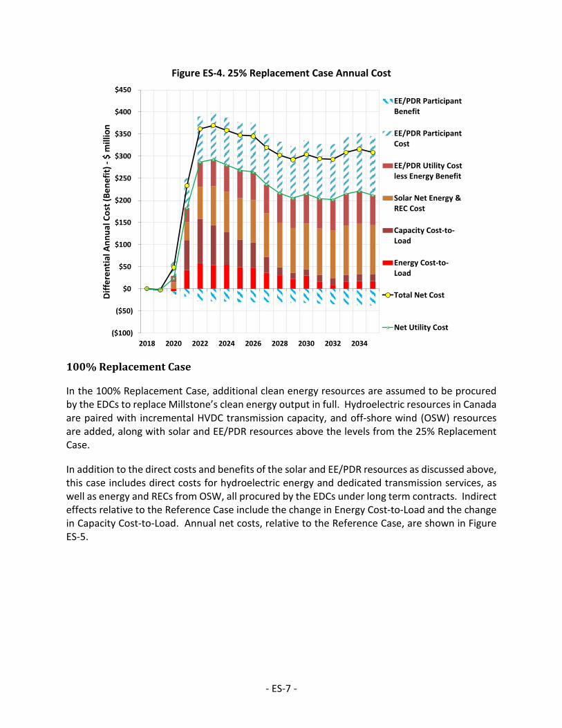
Figure ES-4. 25% Replacement Case Annual Cost
100% Replacement Case
In the 100% Replacement Case, additional clean energy resources are assumed to be procured by the EDCs to replace Millstone’s clean energy output in full. Hydroelectric resources in Canada are paired with incremental HVDC transmission capacity, and off-shore wind (OSW) resources are added, along with solar and EE/PDR resources above the levels from the 25% Replacement Case.
In addition to the direct costs and benefits of the solar and EE/PDR resources as discussed above, this case includes direct costs for hydroelectric energy and dedicated transmission services, as well as energy and RECs from OSW, all procured by the EDCs under long term contracts. Indirect effects relative to the Reference Case include the change in Energy Cost-to-Load and the change in Capacity Cost-to-Load. Annual net costs, relative to the Reference Case, are shown in Figure ES-5.
($100)
($50)
$0
$50
$100
$150
$200
$250
$300
$350
$400
$450
2018 2020 2022 2024 2026 2028 2030 2032 2034
Diff
eren
tial A
nnua
l Cos
t (Be
nefit
) -$
mill
ion
EE/PDR ParticipantBenefit
EE/PDR ParticipantCost
EE/PDR Utility Costless Energy Benefit
Solar Net Energy &REC Cost
Capacity Cost-to-Load
Energy Cost-to-Load
Total Net Cost
Net Utility Cost
- ES-7 -

Figure ES-5. 100% Replacement Case Annual Cost
Comparison of Results
Annual Total Net Cost, relative to the Reference Case, is plotted for each case in Figure ES-6. Total Net Cost includes the participant costs and benefits for the EE/PDR resources in the 25% and 100% Replacement Cases. Figure ES-7 shows a breakout of various cost and benefit components of the differential present value of costs for the replacement cases. Both Net Utility Cost and Total Net Cost are shown.
($200)
$0
$200
$400
$600
$800
$1,000
$1,200
$1,400
2018 2020 2022 2024 2026 2028 2030 2032 2034
Diff
eren
tial A
nnua
l Cos
t (Be
nefit
) -$
mill
ion
EE/PDR ParticipantBenefitEE/PDR ParticipantCostEE/PDR Utility Costless Energy BenefitOSW Net Energyand REC CostSolar Net Energy &REC CostHydro Net EnergyCostTransmission Cost
REC Cost-to-Load
Capacity Cost-to-LoadEnergy Cost-to-Load
Total Net Cost
Net Utility Cost
- ES-8 -

Figure ES-6. Comparison of Annual Total Net Cost
Figure ES-7. Present Value of Total Net Cost
($200)
$0
$200
$400
$600
$800
$1,000
$1,200
2018 2020 2022 2024 2026 2028 2030 2032 2034
Diffe
rent
ial A
nnua
l Cos
t (Be
nefit
) -$
mill
ions
100% Replacement Case25% Replacement Case0% Replacement Case
$719.2
$2,412.3
$6,785.3
$1,794.4
$5,470.9
($1,000)
$0
$1,000
$2,000
$3,000
$4,000
$5,000
$6,000
$7,000
$8,000
0% ReplacementCase
25% ReplacementCase
100% ReplacementCase
Pres
ent V
alue
of D
iffer
entia
l Cos
t (Be
nefit
) -$
mill
ion
EE/PDR ParticipantBenefitEE/PDR ParticipantCostEE/PDR Utility Costless Energy BenefitOSW Net Energyand REC CostSolar Net Energy &REC CostHydro Net EnergyCostTransmission Cost
REC Cost-to-Load
Capacity Cost-to-LoadEnergy Cost-to-Load
Total Net Cost
Net Utility Cost
- ES-9 -

The costs shown in the above charts can be expressed in terms of levelized 2017 dollar cost per MWh of Connecticut load. This reporting convention represents the incremental cost per MWh borne by Connecticut load. For the 0% Replacement Case, the levelized 2017 dollar cost borne by Connecticut load is only $2.02/MWh. The incremental cost burden borne by Connecticut load for the 25% Replacement Case and the 100% Replacement Case is $7.16/MWh and $21.32/MWh, respectively.
ECONOMIC IMPACT ANALYSIS
The postulated retirement of Millstone in 2021 could impair the economic vitality of Connecticut as Dominion’s annual payroll and capital spend, adjusted for income multiplier effects, amount to roughly $350 million per year (2017 $). In performing an economic analysis of this exposure, LAI notes that the lion’s share of the adverse economic impact attributable to Millstone’s retirement theoretically relates to lost income associated with laid off employees. While in theory the lost income and accompanying income multiplier effect across multiple business sectors could be injurious to Connecticut’s economic well-being, LAI believes that the probable outcome is a small adverse financial impact, not a material one. This is because the likelihood is high that the majority of Millstone’s trained workforce would soon be reabsorbed by thriving defense contractors in search of skilled local labor, perhaps all. That Millstone’s workforce is stocked with engineers, tradespeople, and other professionals with security clearances would be of immediate use by prominent defense contractors who have undertaken advanced research and manufacturing initiatives under multi-year Department of Defense contracts.
Adverse economic exposure in the Town of Waterford several years after Millstone’s retirement is another matter, however. The Town has benefited from Millstone’s presence for decades. Millstone pays Waterford about $30 million per year, nearly one-third of the Town’s existing annual budget. Millstone’s retirement would likely create fiscal challenges for the Town of Waterford. How the State of Connecticut and the Town of Waterford might redress or otherwise mitigate these challenges has not been part of this inquiry.
- ES-10 -

1 WHOLESALE ELECTRICITY MARKET IN NEW ENGLAND
Millstone’s revenues are derived from the sale of two electricity products: electric energy and capacity. For the most part, Millstone does not participate in the sale of ancillary services administered by ISO-NE.1 Hence, the sale of energy and capacity through the respective ISO-NE wholesale markets comprise the product slate of relevance over the planning horizon. LAI developed forecasts for market energy and capacity prices that Millstone would earn over an 18-year period. The relevant planning horizon is 2018 to 2035. The period 2018 through 2021 represent “bridge years,” that is, the period corresponding to Millstone’s existing capacity supply obligation to ISO-NE. The remainder of the planning horizon is the period deemed at risk if Dominion were to decide to retire Millstone as soon as 2021. The end of the forecast period coincides with the end of Millstone Unit 2’s current operating license.
In Dominion’s response to an information request from DEEP / PURA, Dominion indicated that the Millstone retirement decision would not separate Unit 2 from Unit 3.2 Hence, in performing this analysis LAI has assumed that Dominion would continue to operate both units or otherwise submit a delist bid to ISO-NE for the retirement of the entire plant. In structuring the analysis framework LAI has assumed continued Millstone operation over a long term planning horizon. The planning horizon of relevance is mid-year 2021 through mid-year 2035. Millstone Unit 2 has an NRC license through 2035. Although Millstone Unit 3 has an NRC license through 2045, LAI has not evaluated the financial performance of Millstone Unit 3 after 2035. The bridge years from 2018 through 2021 have also been examined, but do not enter into the retirement decision in light of Millstone’s Capacity Supply Obligation (CSO) through FCA #11.
The Reference Case represents LAI’s assessment of Millstone’s performance under business-as-usual conditions. To evaluate financial upsides and downsides relative to the Reference Case, a number of sensitivities have been formulated. Tracking lower than anticipated delivered gas prices, LAI has defined a Low Gas Price Case. Tracking higher than anticipated delivered gas prices, LAI has defined a High Gas Price Case. Also, LAI has tested the effect of high renewable energy penetration in New England under a High RE Development Case. Finally, an Electric Vehicle (EV) Penetration Case has been defined to test potential energy sales upside attributable to the potential rapid EV expansion in New England.
In this section, we present the key building block assumptions incorporated in LAI’s electric production simulation model. We also discuss the building block assumptions incorporated in LAI’s gas simulation model. Following the discussion of key factor inputs to the production simulation model, we present the key building block assumptions in the FCM financial model used to forecast capacity prices under ISO-NE’s FCA. The results of the financial analysis are then
1 According to Dominion, both units do receive revenue for reactive power capability under Schedule 2 of the ISO-NE OATT. See Dominion response #11, September 19, 2017. 2 See Dominion letter to Commissioner Klee and Chairwoman Dykes, September 1, 2017, in which Dominion states it has “no intention of retiring one Millstone unit and leaving the other unit operational, and cannot presently foresee a scenario where this would occur.”
- 1 -

presented for Millstone’s continued operation through 2035 under the Reference Case and an array of sensitivities.
1.1 ENERGY FORECAST
LAI utilized AURORAxmp, a chronological dispatch simulation model licensed from EPIS, Inc., to forecast wholesale electric energy prices. LAI has utilized AURORAxmp for many commercial and regulatory applications in ISO-NE, NYISO, PJM, MISO, and other parts of the Eastern Interconnection.3
The primary focus for the net cash flow analysis is the derivation of Millstone’s profitability from energy sales in New England over the planning horizon. The energy price forecast therefore required analysis of many factors influencing the energy market, including new resource entry, existing resource retirements, demand-side changes, emission allowance prices, and fuel prices. As natural gas is typically the marginal fuel in ISO-NE, the forecast of delivered natural gas prices is particularly important in light of uncertainty factors about the cost of gas “into-the-pipe,” local distribution company (LDC) growth rates, pipeline improvements into and within New England, and LNG dispatch assumptions. Key factor inputs to the electric and gas simulation models provide a sound foundation for purposes of deriving Millstone’s net margin from energy sales over the forecast period.4 The energy price forecast from AURORAxmp was converted into a nodal price using statistical modeling.
Whereas net cash flow research has been centered on Millstone’s expected profitability assuming continued unit operation, in the replacement cost analysis LAI has examined energy price and emissions effects assuming both Millstone units retire mid-year 2021. Several Millstone replacement scenarios have been defined.
A “0% Replacement Case” has been formulated where LAI makes the simplifying assumption that Connecticut does not mandate substitute technology in Connecticut to mitigate the increase in carbon emissions associated with the postulated loss of Millstone, but new gas resources are added on a merchant basis to the resource mix to meet ISO-NE’s Net ICR.
A “25% Replacement Case” has been formulated where about 25% of Millstone’s energy output each year is met through the addition of solar and DR/EE in Connecticut. 25% represents Connecticut’s load share of Millstone.
A “100% Replacement Case” has been formulated where Millstone’s energy output is replaced with an array of renewable and clean energy technologies in both Connecticut and elsewhere in New England following the postulated Millstone retirement.
3 From 2013 through 2015, LAI performed a gas/electric interdependency assessment across six participating planning authorities for PJM, ISO-NE, NYISO, MISO, the IESO of Ontario, and TVA. This study was funded by the Department of Energy and was conducted for the Eastern Interconnection Planning Collaborative. 4 Energy prices are derived in AURORAxmp. Derivation of net margin from energy sales accounts for Millstone’s fuel costs and variable O&M expenses, which are addressed in the financial model.
- 2 -

More detail about the technology composition in the 25% and 100% Replacement Cases is presented in section 1.1.3. The energy, capacity and carbon emission effects under each replacement scenario are presented in section 1.1.4.
1.1.1 Reference Case Assumptions (With Millstone)
Study Region
In order to efficiently utilize computing power and analytic resources, LAI ran AURORAxmp in a zonal configuration and set the Study Region modeled in AURORAxmp to include ISO-NE, NYISO, and the MAAC portion of PJM. The MAAC portion of PJM was included as the downstate region of NYISO (including New York City and Long Island) which utilizes energy imports from both New Jersey and Connecticut. Experience has shown that market dynamics in MAAC affect transmission interchange to NYISO, in particular, downstate New York, which would in turn affect interchange between NYISO and ISO-NE (between Connecticut and Long Island). Energy prices in Connecticut may be sensitive to resource changes in all three RTOs. Imports from Canada, which include Quebec, Ontario, and New Brunswick, were modeled based on an average weekly profile for each month using three years of historical flow data (168 hours by 12 months, 2014-2016).
Figure 1. Study Footprint
The three RTOs were further divided into zonal representations to capture transmission constraints within each RTO. ISO-NE was represented as the 13 sub-areas documented in the Regional System Plan (RSP) and other planning documents. NYISO was represented as 11 load zones (A through K). The MAAC portion of PJM was divided into zones based on the Local Delivery Areas (LDAs) represented in the Base Residual Auction, which includes planning parameters such as Capacity Emergency Transfer Limits (CETL) which inform transmission constraints. MAAC was split into Southwest MAAC (SWMAAC), Eastern MAAC (EMAAC), and rest-of MAAC zones.
NYISO
ISO-NE
PJMMAAC
- 3 -

Transmission Limits
Zonal transmission limits were defined using publicly available data sources:
• ISO-NE RSP5
• ISO-NE FCM Tie Benefits Study6
• NYSRC Installed Capacity Requirement (ICR) Report7
• NYISO ESPWG / TPAS meeting materials8
• PJM Base Residual Auction (BRA) Planning Parameters9
In cases where data are not available or data sources conflict, LAI relies on the “default settings” provided by EPIS, the licensor of AURORAxmp, as well as LAI’s judgment to determine appropriate limits.
Demand Forecast
LAI relied on RTO planning documents such as ISO-NE’s CELT Report, NYISO’s Gold Book, and PJM’s Load Forecast Report as the basis for our peak and annual energy forecasts.10 LAI utilized the RTO forecasts that include energy efficiency (EE) and passive demand response (PDR). We assume that the CELT EE/PDR forecast, which is developed in consultation with ISO-NE stakeholders, represents full implementation of Connecticut’s currently authorized Conservation and Load Management programs.
LAI modeled behind-the-meter (BTM) solar, which is forecasted in planning documents, as a supply-side resource in order to reflect the changes to hourly shape of “net load” that solar creates as dispatch cannot track demand. We have assumed that the CELT BTM forecast, which is developed in consultation with ISO-NE stakeholders, implements Connecticut’s RPS requirements.
5 https://www.iso-ne.com/static-assets/documents/2015/11/rsp15_final_110515.docx 6 https://www.iso-ne.com/static-assets/documents/2017/05/a6-3_pspc_may182017_2021_fca_tie_benefits_assumptions.pdf 7 http://nysrc.org/NYSRC_NYCA_ICR_Reports.html 8 http://www.nyiso.com/public/markets_operations/committees/meeting_materials/index.jsp?com=bic_espwg http://www.nyiso.com/public/markets_operations/committees/meeting_materials/index.jsp?com=oc_tpas 9 http://pjm.com/markets-and-operations/rpm.aspx 10 CELT: https://iso-ne.com/system-planning/system-plans-studies/celt Gold Book: http://www.nyiso.com/public/webdocs/markets_operations/services/planning/Documents_and_Resources/Planning_Data_and_Reference_Docs/Data_and_Reference_Docs/2017_Load_and_Capacity_Data_Report.pdf Load Forecast Report: http://pjm.com/-/media/library/reports-notices/load-forecast/2017-load-forecast-report.ashx?la=en
- 4 -

Figure 2. 2017 CELT Annual Energy Demand Forecast
Since the Study Period is longer than the ten and fifteen-year forecasts that RTOs provide, LAI assumed that the gross load (not net of EE/PDR or BTM solar) grows at a rate equal to the last forecasted annual growth rate for the rest of the Study Period. EE/PDR and BTM solar were assumed to grow at a constant MW/MWh rate based on the last forecasted difference for the rest of the Study Period.
Fuel Price Forecast
In this section, LAI reviews the structure and assumptions used to forecast delivered natural gas prices, oil and coal. Uranium prices are not relevant in New England for purposes of deriving energy prices. This is because LAI has assumed that nuclear units are always price takers, not price setters.11 Nevertheless, in section 3.4 we review uranium price trends for the industry as a whole in the narrow context of uranium price trends affecting Millstone’s financial exposure under stress test assumptions.
Gas Price Forecast
Gas commodity prices at Henry Hub are forecasted using NYMEX pricing for 2018 and 2019, and 2017 U.S. Energy Information Administration (EIA) Annual Energy Outlook (AEO) Reference case prices from 2020 through 2035. Monthly shaping was applied to the annual AEO forecast based
11 Nuclear plants generally have limited dispatch flexibility and cannot withhold a significant amount of generation capability in the event that energy prices are lower than variable (including fuel) costs.
0
20,000
40,000
60,000
80,000
100,000
120,000
140,000
160,000
180,000
2017 2018 2019 2020 2021 2022 2023 2024 2025 2026
Ener
gy (G
Wh)
Gross
Net PDR
Net PDR, PV
- 5 -

on ten years of historical Henry Hub prices. The resultant commodity price forecast is shown in Figure 3.
Figure 3. Henry Hub Gas Commodity Price Forecast
The NYMEX futures values are used through 2019 due to limited liquidity beyond that point. While NYMEX is a reasonable basis for tracking the value of natural gas into-the-pipe at the Henry Hub over the short term, because market participants do not significantly trade the forward index, it is of limited value as a relevant price benchmark over the intermediate to long term. Figure 4 shows the NYMEX trading activity around Henry Hub futures on September 20, 2017, the date of the strip that is used in the gas price forecast. While NYMEX reports futures settlements through 2029, trading volumes and open interest are significantly diminished beyond the first 24 to 30 months of a given daily strip.
$0
$1
$2
$3
$4
$5
$6Ja
n-18
Jan-
19
Jan-
20
Jan-
21
Jan-
22
Jan-
23
Jan-
24
Jan-
25
Jan-
26
Jan-
27
Jan-
28
Jan-
29
Jan-
30
Jan-
31
Jan-
32
Jan-
33
Jan-
34
Jan-
35
Gas
Com
mod
ity F
orec
ast
(201
7 $/
MM
Btu)
Shift from NYMEX to AEO
- 6 -

Figure 4. NYMEX Trading Activity
In the AEO 2017 Reference case, natural gas production, illustrated in Figure 5, is projected to grow at about 4% per year through 2020. New petrochemical plants and LNG export terminals built in response to low natural gas prices support the near-term production growth, but are reduced as prices rise. Production growth decreases to 1% per year after 2020 as net exports level out, domestic consumption becomes more efficient, and prices slowly rise as the result of increased drilling levels and production expansion into more expensive areas.
0
50,000
100,000
150,000
200,000
250,000
300,000
Oct
-17
Jan-
18
Apr-
18
Jul-1
8
Oct
-18
Jan-
19
Apr-
19
Jul-1
9
Oct
-19
Jan-
20
Apr-
20
Jul-2
0
Oct
-20
Jan-
21
Apr-
21
Jul-2
1
Oct
-21
Trad
ing
Activ
ity
Futures Month
Open Interest
Total Volume
- 7 -

Figure 5. Reference Case Dry Gas Production
Production from shale gas and associated gas from tight oil plays is projected to be the source of nearly two-thirds of total domestic gas production by 2035. The Marcellus and Utica plays are the main driver of growth in shale production; the contribution of Eastern shale plays to total production in shown in Figure 6.
0
20
40
60
80
100
120
2000 2005 2010 2015 2020 2025 2030 2035
U.S
. Dry
Nat
ural
Gas
Pro
duct
ion
(Bcf
/d)
History
Reference case
- 8 -

Figure 6. Reference Case Gas Production by Source
Despite decreasing in the near term, natural gas consumption is expected to increase during much of the projection period, as shown in Figure 7. The industrial sector, including LNG production, is the largest consumer of natural gas during most years of the forecast. Reference case prices rise modestly from 2020 through 2030 as electric power sector gas consumption increases, but stay relatively flat after 2030 as technology improvements keep pace with rising demand. Residential and commercial sector gas consumption remains largely flat over the forecast period as a result of efficiency gains that balance increases in the number of housing units and commercial floor space.
- 9 -

Figure 7. Reference Case Gas Consumption by Sector
]
LNG exports, shown in Figure 8, are projected to dominate U.S. natural gas exports by the early-2020s. The first LNG export facility in the Lower 48, Sabine Pass, began operations in 2016, and four more LNG export facilities are scheduled to be completed by 2020. After 2020, U.S. exports of LNG grow at a more modest rate as U.S.-sourced LNG becomes less competitive in global energy markets.
- 10 -

Figure 8. Reference Case LNG Exports
Basis differentials for delivered gas prices are forecasted using GPCM, an industry standard linear programming model licensed from RBAC, Inc. New England-specific inputs include forecasts of LDC demand, LNG imports, and pipeline infrastructure additions into and within New England. The forecast of utility gas demand is based on state filings from LDCs across New England. The forecast of LNG imports is based on historical LNG imports, specifically from the winter of 2015-16. The Reference Case forecast includes the Connecticut Expansion Project, the Atlantic Bridge Project, and the Continent-to-Coast Project in the project infrastructure. In order to ensure that New England’s gas infrastructure is sufficient to serve residential, commercial and industrial gas demand over the forecast horizon, additional incremental expansions have been added where need is indicated by GPCM.12 These incremental expansions have the effect of reducing winter basis spikes which would otherwise begin to appear again in early 2024 as the recent pipeline expansions become fully utilized.13 The resultant delivered gas price forecast, represented by Algonquin Citygates, is shown in Figure 9.
12 The incremental expansions include an 80 MDth/d expansion of Algonquin from Connecticut into Rhode Island in November 2020, a 31 MDth/d expansion of Algonquin from Rhode Island into Massachusetts in February 2021, a 65 MDth/d expansion of Tennessee from southeast New York into Connecticut in January 2030, a 21 MDth/d expansion of Tennessee’s NH lateral in January 2033, and a 58 MDth/d expansion of the Brookfield interconnection from Algonquin to Iroquois. 13 The optimization model does not consider or calculate the costs associated with constructing the expansions. The cost of these expansions has not been included in the financial modeling because it is assumed to be borne by the contracting LDCs.
- 11 -

Figure 9. Delivered Gas Price Forecast
Oil Price Forecast
Our forecast of delivered oil product prices starts with NYMEX forward price curves for domestic crude oil and for ultra-low-sulfur diesel (ULSD), the primary backup fuel for gas-fired plants. The NYMEX crude and ULSD prices extend through December 2025 and January 2021, respectively; LAI extends those price projections based on the 2017 AEO. LAI derives the Residual Fuel Oil price based on its historical correlation to crude oil prices.
Historically, oil-fired generation in ISO-NE has mostly run in the winter when gas prices spike during cold snaps. Occasionally, oil-fired generation runs during the non-winter season during outage contingencies or pipeline maintenance periods. Since LAI utilized a monthly gas price forecast, oil-fired generation was observed to be rarely in merit. Oil-fired generators are generally less efficient, face higher non-fuel O&M costs, and have higher carbon emission rates than gas-fired generators. Therefore gas/oil price parity alone will not place oil resources in merit -- oil-fired generation needs to be economic at the margin to offset these other dispatch costs.
$0
$2
$4
$6
$8
$10
$12
Jan-
18
Jan-
19
Jan-
20
Jan-
21
Jan-
22
Jan-
23
Jan-
24
Jan-
25
Jan-
26
Jan-
27
Jan-
28
Jan-
29
Jan-
30
Jan-
31
Jan-
32
Jan-
33
Jan-
34
Jan-
35
AGT
CG D
eliv
ered
For
ecas
t (2
017
$/M
MBt
u)
- 12 -

Figure 10. Oil Products Price Forecast
Coal Price Forecast
Coal prices are forecasted using the 2017 STEO and AEO prices for delivered coal to electric generators as a commodity price. These prices are then adjusted on a unit and state level to reflect local price adders based on basin sourcing and transportation costs. These adders are developed by EPIS Inc. and primarily based on a review of EIA-923 fuel receipts data.
- 13 -
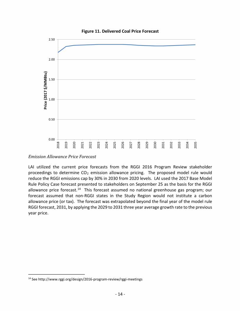
Figure 11. Delivered Coal Price Forecast
Emission Allowance Price Forecast
LAI utilized the current price forecasts from the RGGI 2016 Program Review stakeholder proceedings to determine CO2 emission allowance pricing. The proposed model rule would reduce the RGGI emissions cap by 30% in 2030 from 2020 levels. LAI used the 2017 Base Model Rule Policy Case forecast presented to stakeholders on September 25 as the basis for the RGGI allowance price forecast.14 This forecast assumed no national greenhouse gas program; our forecast assumed that non-RGGI states in the Study Region would not institute a carbon allowance price (or tax). The forecast was extrapolated beyond the final year of the model rule RGGI forecast, 2031, by applying the 2029 to 2031 three year average growth rate to the previous year price.
14 See http://www.rggi.org/design/2016-program-review/rggi-meetings
0.00
0.50
1.00
1.50
2.00
2.50
2018
2019
2020
2021
2022
2023
2024
2025
2026
2027
2028
2029
2030
2031
2032
2033
2034
2035
Pric
e (2
017
$/M
MBt
u)
- 14 -
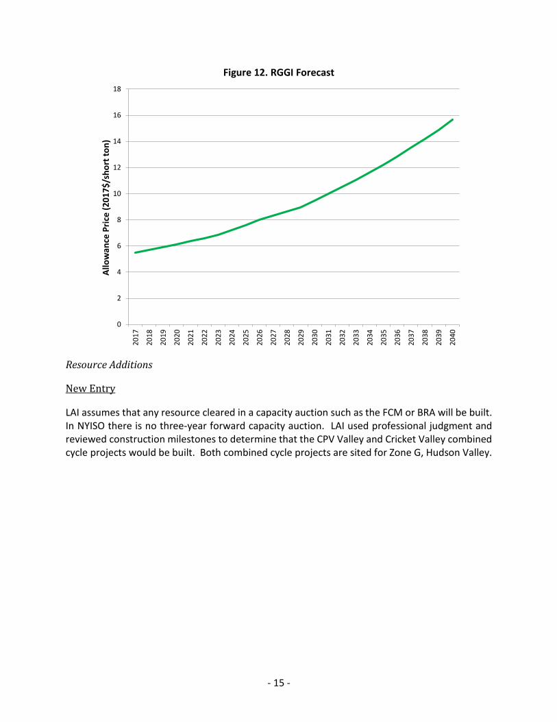
Figure 12. RGGI Forecast
Resource Additions
New Entry
LAI assumes that any resource cleared in a capacity auction such as the FCM or BRA will be built. In NYISO there is no three-year forward capacity auction. LAI used professional judgment and reviewed construction milestones to determine that the CPV Valley and Cricket Valley combined cycle projects would be built. Both combined cycle projects are sited for Zone G, Hudson Valley.
0
2
4
6
8
10
12
14
16
18
2017
2018
2019
2020
2021
2022
2023
2024
2025
2026
2027
2028
2029
2030
2031
2032
2033
2034
2035
2036
2037
2038
2039
2040
Allo
wan
ce P
rice
(201
7$/s
hort
ton)
- 15 -

CPV Valley (680 MW) is expected to be online in early 2018.15,16 Cricket Valley (1,100 MW) is expected to be in service by 2020, with site work and transmission upgrades underway.17
For renewable resources, LAI assumes that projects with signed ISAs in ISO-NE or PJM or accepted interconnection cost allocations in NYISO will be built.18
Policy Additions
LAI assumes that offshore wind (OSW) projects with approved contracts are built. The Maryland PSC recently approved the procurements for the US Wind and Skipjack projects, a combined 368 MW of OSW capacity. The Long Island Power Authority recently contracted with the 90 MW Deepwater South Fork project as part of its most recent renewable RFP. In addition to these contracts, we assume that the Massachusetts 83C procurement will culminate in the full development of 1,600 MW of OSW.19 LAI has assumed that New York State through NYSERDA will develop 800 MW of OSW in the downstate area to meet its Energy Master Plan.
LAI has also assumed that Massachusetts will procure clean energy resources in its 83D procurement. We assume that an HVDC project will be built to provide incremental hydropower
15 http://www.recordonline.com/news/20170514/900m-orange-county-power-plant-moves-closer-to-completion 16 One uncertainty factor affecting startup of CPV Valley is the status of the dedicated 8-mile gas lateral from Millennium. FERC authorized the project on November 9, 2016. Following FERC authorization, the NYSDEC sent a letter to Millennium stating that the one-year review clock for the project’s water quality permit application began when the application was deemed complete on August 31, 2016, rather than when the application was initially received on November 23, 2015. On July 21, 2017, Millennium submitted a request to proceed with construction on the basis of their assertion that NYSDEC had waived its right to issue the water quality permit following a finding of lack of standing from the D.C. Circuit Court of Appeals with the explanation that Millennium could seek a waiver from FERC. On August 30, 2017, NYSDEC denied the water quality permit, on the basis that the environmental review is incomplete because FERC had failed to consider the effects of downstream greenhouse gas emissions. On September 15, 2017, FERC issued Millennium a waiver of the NYSDEC Section 401 water permit due to NYSDEC’s failure to act on the permit application within one year of submission. NYSDEC requested rehearing of the waiver decision. FERC authorized Millennium to begin construction on the Valley Lateral facilities on October 27, 2017. On October 30, 2017, NYSDEC requested that FERC stay the construction authorization pending the rehearing decision, and also requested an emergency stay from the 2nd Circuit Court of Appeals, since it could not file a petition with the Court until the rehearing request was resolved. The 2nd Circuit granted an administrative stay on November 2, 2017. On November 16, 2017, FERC denied NYSDEC’s rehearing request, and on November 17, 2017, NYSDEC filed a petition with the 2nd Circuit for review of FERC’s water quality permit waiver decision and denial of rehearing. Oral arguments took place on December 5, 2017. On December 7, 2017, the 2nd Circuit denied the request for a stay of construction and planned for expedited review of the case, which could be heard as early as late January 2018. 17 http://www.cricketvalley.com/news.aspx 18 Despite having an executed ISA, LAI excluded Cape Wind since its contracts with Eversource and NGrid have been terminated. 19 MA DOER may direct the EDCs to enter into contracts up to 800 MW in the first solicitation, but not less than 400 MW provided the first 400 MW tranche is deemed cost effective. In defining the OSW buildout profile in New England, LAI has made the simplifying assumption that there are four 400 MW tranches of OSW added in two year intervals, thereby resulting in 1,600 MW by 2027/28.
- 16 -

and wind imports from Quebec. We also assume that Massachusetts will meet its storage initiative goal to procure 200 MWh of storage capacity by 2020.
Renewable Portfolio Standards
We assumed that all Class 1/Tier 1 renewable energy requirements in every state within the study region were met in 2016 and estimated the Class 1/Tier 1 energy additions needed to meet Class 1/Tier 1 renewable portfolio standards through 2035. Annual requirements for each state are shown in Figure 13 and Figure 14.
Figure 13. NE States RPS Class 1/Tier 1 Requirements
0
10
20
30
40
50
60
70
80
90
2017 2019 2021 2023 2025 2027 2029 2031 2033 2035
Tier
1 R
E (%
of R
etai
l Sal
es)
CT MA ME NH RI VT
- 17 -

Figure 14. Non-NE States RPS Class 1/Tier 1 Requirements
In New England, with the assumed resource additions, no additional generic Class 1/Tier 1 energy is needed to meet future RPS or Massachusetts’ Clean Energy Standard annual requirements. In New York, we estimated the energy needed to meet the future state’s Clean Energy Standard annual goals. In PJM, we estimated the energy needed to meet the future Class 1/Tier 1 RPS annual goals within the MAAC states.
Generic utility scale and land based wind energy was added to make up the Class 1/Tier 1 energy deficit for New York and PJM. The solar to wind ratio used is the same ratio found in the RTOs’ interconnection queues. Generic utility scale solar additions were distributed to zones in proportion to the zonal peak demand and generic land based wind additions were distributed in proportion to zonal queued wind capacity that has not already been included in the AURORA model.
Resource Adequacy Additions
Once all other postulated resource additions and retirements are determined, LAI determines whether each RTO and associated capacity zones or Local Deliverability Areas meet resource adequacy requirements. LAI extrapolates resource adequacy requirements primarily based on peak load forecasted in each RTO’s load forecast and then compares the requirement to the available supply in each delivery period. LAI did not find any resource adequacy shortfalls in ISO-NE or PJM. However, NYISO Zone J (and the New Capacity Zone it is nested in) experienced a
0
10
20
30
40
50
60
2017 2019 2021 2023 2025 2027 2029 2031 2033 2035
Tier
1 R
E (%
of R
etai
l Sal
es)
NY DC DE MD NJ PA VA
- 18 -
shortfall. LAI added new resources modeled on the CONE combined cycle and combustion turbine units studied in the Demand Curve Reset in order to meet local requirements.
Resource Retirements
Firm Retirements
Our forecast includes retirements documented by the RTOs in planning documents and notices. ISO-NE de-list bids through FCA 11 and non-price retirements are reflected in the resource mix. NYISO retirement notices and PJM deactivations lists through end of September 2017 are also integrated into the retirement assumptions.
We also assume that per the New York State’s mandate, Indian Point units 2 and 3 retire in 2020 and 2021, respectively. None of the other nuclear facilities in New York are expected to retire during the Study Period.
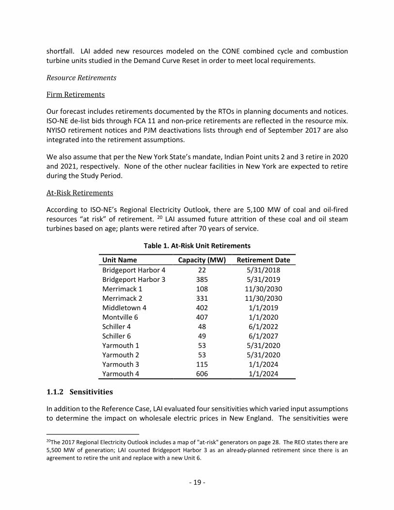
At-Risk Retirements
According to ISO-NE’s Regional Electricity Outlook, there are 5,100 MW of coal and oil-fired resources “at risk” of retirement. 20 LAI assumed future attrition of these coal and oil steam turbines based on age; plants were retired after 70 years of service.
Table 1. At-Risk Unit Retirements
Unit Name Capacity (MW) Retirement Date Bridgeport Harbor 4 22 5/31/2018 Bridgeport Harbor 3 385 5/31/2019 Merrimack 1 108 11/30/2030 Merrimack 2 331 11/30/2030 Middletown 4 402 1/1/2019 Montville 6 407 1/1/2020 Schiller 4 48 6/1/2022 Schiller 6 49 6/1/2027 Yarmouth 1 53 5/31/2020 Yarmouth 2 53 5/31/2020 Yarmouth 3 115 1/1/2024 Yarmouth 4 606 1/1/2024
1.1.2 Sensitivities
In addition to the Reference Case, LAI evaluated four sensitivities which varied input assumptions to determine the impact on wholesale electric prices in New England. The sensitivities were
20The 2017 Regional Electricity Outlook includes a map of "at-risk" generators on page 28. The REO states there are 5,500 MW of generation; LAI counted Bridgeport Harbor 3 as an already-planned retirement since there is an agreement to retire the unit and replace with a new Unit 6.
- 19 -

determined in consultation with DEEP/PURA to represent discrete energy futures. They are not intended to fully bookend the range of possible market outcomes, but rather to individually test different drivers in input assumptions.
High Gas Price
The High Gas Price Case assumes a gas commodity price based on the 2017 AEO Low Oil and Gas Resource and Technology case, shown relative to the Reference Case gas commodity forecast in Figure 15.
Figure 15. Gas Commodity Price Forecast, High Gas Price Case
In the AEO 2017 Low Oil and Gas Resource and Technology case, higher costs and lower resource availability result in decreased levels of production, illustrated in Figure 16, at higher prices. These higher prices also have a reductive effect on consumption (Figure 17), and LNG exports (Figure 18).
$0
$1
$2
$3
$4
$5
$6
$7
$8
$9
$10
Jan-
18
Jan-
19
Jan-
20
Jan-
21
Jan-
22
Jan-
23
Jan-
24
Jan-
25
Jan-
26
Jan-
27
Jan-
28
Jan-
29
Jan-
30
Jan-
31
Jan-
32
Jan-
33
Jan-
34
Jan-
35
Gas
Com
mod
ity F
orec
ast
(201
7 $/
MM
Btu)
Reference Case High Gas Price Case
- 20 -

Figure 16. Dry Gas Production, High Gas Price Case
Figure 17. Gas Consumption by Sector, High Gas Price Case
- 21 -

Figure 18. LNG Exports, High Gas Price Case
The basis forecast for the High Gas Price Case assumes that lower gas demand and higher LNG imports will results from the higher commodity price forecast. Gas infrastructure in New England is unchanged from the Reference Case. The resultant delivered gas price forecast, represented by Algonquin Citygates, is shown in Figure 19.
- 22 -

Figure 19. Delivered Gas Price Forecast, High Gas Price Case
Low Gas Price
The Low Gas Price Case assumes a gas commodity price based on the 2017 AEO High Oil and Gas Resource and Technology case, shown relative to the Reference Case gas commodity forecast in Figure 20.
$0
$2
$4
$6
$8
$10
$12
Jan-
18
Jan-
19
Jan-
20
Jan-
21
Jan-
22
Jan-
23
Jan-
24
Jan-
25
Jan-
26
Jan-
27
Jan-
28
Jan-
29
Jan-
30
Jan-
31
Jan-
32
Jan-
33
Jan-
34
Jan-
35
AGT
CG D
eliv
ered
For
ecas
t (2
017
$/M
MBt
u)Reference Case High Gas Price Case
- 23 -

Figure 20. Gas Commodity Price Forecast, Low Gas Price Case
In the AEO 2017 High Oil and Gas Resource and Technology case, lower costs and higher resource availability result in increased levels of production, illustrated in Figure 21.
$0
$1
$2
$3
$4
$5
$6
Jan-
18
Jan-
19
Jan-
20
Jan-
21
Jan-
22
Jan-
23
Jan-
24
Jan-
25
Jan-
26
Jan-
27
Jan-
28
Jan-
29
Jan-
30
Jan-
31
Jan-
32
Jan-
33
Jan-
34
Jan-
35
Gas
Com
mod
ity F
orec
ast (
2017
$/M
MBt
u)Reference Case Low Gas Price Case
- 24 -

Figure 21. Dry Gas Production, Low Gas Price Case
As in the AEO 2017 Reference case, Eastern shale production, shown in Figure 22, is the primary driver of production growth over the forecast horizon. The availability of increased production at lower prices in this AEO 2017 case also increases domestic consumption (Figure 23), and makes U.S. LNG exports more competitive with other global suppliers (Figure 24).
- 25 -

Figure 22. Eastern Shale Production, Low Gas Price Case
Figure 23. Gas Consumption by Sector, Low Gas Price Case
- 26 -

Figure 24. LNG Exports, Low Gas Price Case
The basis forecast for the Low Gas Price Case assumes that higher gas demand and lower LNG imports will result from the lower commodity price forecast. Additionally, Enbridge’s Access Northeast Project is assumed to be commercialized in phases between 2021 and 2024. The resultant delivered gas price forecast, represented by Algonquin Citygates, is shown in Figure 25.
- 27 -

Figure 25. Delivered Gas Price Forecast, Low Gas Price Case
High RE Development
The High RE Development Case assumes approximately 6 TWh / year of incremental renewable energy from about 1,850 MW of wind and solar resources located in northern New England. This represents about 5% of metered load in New England. These projects are currently in the ISO-NE queue and are included in ISO-NE’s economic analysis of transmission upgrades needed to interconnect these resources.21 We assumed that a 1,471 MW HVDC transmission line from Maine to Central Massachusetts would need to be constructed to mitigate congestion between Northern and Southern New England, as postulated in an ISO-NE economic study.22
EV Penetration
In the EV Penetration Case we assumed the same levels of Plug-in EVs that ISO-NE assumed in Sensitivity Case 3 of their 2016 economic study.23 We assumed linear growth to the 2025 and 2030 EV penetration assumptions, with EV growth starting in 2019 and extrapolating growth from 2030 on based on the 2025 to 2030 annual growth rate.
21 https://www.iso-ne.com/static-assets/documents/2017/07/a3_maine_resource_integration_study_scenarios _and_cost_estimated.pdf 22 https://www.iso-ne.com/static-assets/documents/2016/10/2016_economic_studies_high_level_transmission _costs_rev1.pdf 23 https://www.iso-ne.com/static-assets/documents/2016/06/a9_2016_economic_study_assumptions.pdf
$0
$2
$4
$6
$8
$10
$12
Jan-
18
Jan-
19
Jan-
20
Jan-
21
Jan-
22
Jan-
23
Jan-
24
Jan-
25
Jan-
26
Jan-
27
Jan-
28
Jan-
29
Jan-
30
Jan-
31
Jan-
32
Jan-
33
Jan-
34
Jan-
35
AGT
CG D
eliv
ered
For
ecas
t (2
017
$/M
MBt
u)Reference Case Low Gas Price Case
- 28 -

Figure 26. PHEV Growth Assumptions, ISO-NE
Like ISO-NE's approach, EVs were modeled as daily demand resources that are charged during off-peak periods (HE24-HE7) and are assumed to have constant daily demand. ISO-NE's exact charging profile is not tabulated; AURORAxmp solved for which hours to charge. This case added about 7% of off-peak power demand over the course of the study period (~14% demand increase in 2035).
1.1.3 Retirement Analysis
LAI assumed that in the retirement cases both Millstone units retired effective May 31, 2021. Millstone is committed in FCM through the 2020-21 delivery year. Due to the size of Millstone’s CSO and the very limited liquidity in ISO-NE’s reconfiguration auction, LAI has made the simplifying assumption that it would be prohibitively expensive for Dominion to unwind the Millstone CSO in the reconfiguration auction(s) for such large resources. EnergyZT estimated that the cost to Dominion to buy out of its existing Millstone CSOs would be around $680 million.24 The high anticipated cost of unwinding Millstone’s CSO through FCA #11 renders moot the examination of Millstone’s potential retirement before the 2021-22 delivery year.
In consultation with DEEP / PURA, LAI formulated three Millstone replacement scenarios: a 0% clean energy replacement case, a 25% clean energy replacement case (Connecticut’s load share of Millstone), and a 100% clean energy replacement case. Each replacement scenario has been
24 “Millstone Power Plant: Estimated Cost to Exit Capacity Supply Obligations”, October 2017, EnergyZT Advisors
0
1
2
3
4
5
6
7
2018
2019
2020
2021
2022
2023
2024
2025
2026
2027
2028
2029
2030
2031
2032
2033
2034
2035
PHEV
s (M
illio
ns)
- 29 -

tested in AURORAxmp to calibrate the increased duty on the existing fleet of gas-fired generation in New England, as well as any need for additional combined cycle plants to meet the Net ICR. As discussed in section 4, LAI then performed financial analysis of the incremental cost borne by Connecticut load under each of the replacement scenarios designed to support Connecticut’s GWSA goals.
Connecticut’s Local Sourcing Requirement / Transmission Security Analysis
DEEP / PURA asked ISO-NE to provide guidance about Connecticut’s Local Sourcing Requirement (LSR) and the region’s exposure to a net installed capacity requirement (ICR) deficiency if Millstone were excluded from the resource mix in FCA #12. On September 15, 2017, ISO-NE provided DEEP/PURA with a technical response to the question of how retirement of the Millstone units would affect resource adequacy in Connecticut and the region.25 Prior to reviewing the ISO-NE report, LAI was concerned that loss of Millstone would result in a shortfall for Connecticut’s LSR.
ISO-NE found that the LSR calculation for the 2021-2022 delivery year did not significantly change with the postulated removal of the Millstone units. LSR is defined as the greater value of two calculations that ISO-NE performs: the Transmission Security Analysis (TSA) and the Local Resource Adequacy (LRA) requirement. ISO-NE found that the TSA value, calculated using a loss-of-load analysis, was greater than the LRA value absent Millstone. Since the TSA value is easier to forecast and estimate (and was found to be the binding constraint for LSR) LAI projected the TSA value over the Study Period.
ISO-NE calculated TSA using a simple formula which takes the 90/10 local demand forecast net of PV generation, adjusts it for contingencies and import limits, and pro-rates the requirement based on existing generators’ expected outage rates. The ISO-NE response showed that import limits would not change absent the Millstone units, but the “line-line” analysis would be used instead of “line-gen” in the TSA calculation.26
Since Dominion’s ownership, the Millstone units have had very low forced outage rates. Removing the Millstone units from the resource mix increased the weighted average forced outage rate of the remaining Connecticut resources, which offset the decrease in requirement from line-line analysis and created a slight net increase in the TSA. Overall, these changes only yielded a net increase in LSR of 59 MW (from 6,515 MW with Millstone to 6,574 MW without Millstone) in ISO-NE’s calculated requirement for the FCA #12 delivery year. Even absent Millstone, Connecticut has 8,060 MW of existing resources remaining according to ISO-NE.
25 See ISO-NE response to Commissioner Klee and Chairwoman Dykes, “Representative Connecticut Local Sourcing Requirements for 2021-2022 with and without Millstone Nuclear Power Station,” September 15, 2017. 26 This means that the 2,200 MW (N-1-1) transmission limit would be subtracted from the 90/10 demand, rather than adding the largest single source contingency (which normally is Millstone Unit 3 at 1,225 MW) to the requirement and subtracting the 3,400 (N-1) limit. This change from line-gen to line-line analysis yielded a net decrease in the requirement of 25 MW.
- 30 -

Our long-term projections did not find an LSR shortfall over the Study Period, since the LSR did not materially increase absent Millstone. We therefore assumed that the TSA analysis with line-line adjustments was used in all subsequent delivery years and that the N-1-1 import limit remained constant over the forecast period. We extrapolated the TSA calculation for future years using the 90/10 demand forecast net of PV from the load forecast and assume limited changes to outage rates.
However, gas-fired resources are still needed to meet ISO-NE’s pool-wide ICR. Thus, unlike in the Reference Case, the replacement cases require replacement capacity in order to meet resource adequacy requirements. Millstone Unit 3 has a summer capacity rating of 1,225 MW. As such, it constitutes the second largest single contingency considered for system reliability studies. ISO-NE operates its system to maintain reliability in the event of a major contingency, i.e., a generation or transmission failure. If Millstone were to retire in 2021, ISO-NE would plan around system reconfiguration under its N-1-1 criterion. Exactly what planning protocols would be implemented and how are outside the scope of this inquiry. If Millstone were to retire, transmission limits may be encountered more frequently, thereby increasing congestion. The magnitude and frequency of such congestion has not been evaluated in this study. Likewise, whether or not transmission improvements would be required to safeguard grid reliability absent Millstone has not been evaluated.
0% Replacement
In the 0% Replacement Case, no new clean energy resources are added to mitigate the loss of zero-carbon output that Millstone provides. No additional pipeline capacity is contemplated in the Millstone replacement analysis even though existing pipeline constraints would likely be of longer duration and more frequent throughout the heating season.
As previously discussed, the postulated loss of Millstone creates a capacity deficit in ISO-NE, but not in Connecticut. To meet the Net ICR, LAI has made the simplifying assumption that new gas-fired resources will be added under the FCA to ensure resource adequacy.27 In our buildout, the second unit of the Clear River Energy Center in Rhode Island was assumed to be the first resource added to mitigate capacity shortfalls.28 After Clear River Unit 2, LAI has assumed that generic combined cycle capacity in Connecticut is added to mitigate subsequent shortfalls. Other than Clear River Unit 2, we have not contemplated the addition of new generic combined cycle plants elsewhere in New England. Connecticut makes the most sense for siting since Northern New England can be export constrained and is comparatively far from load. The addition of new resources in Massachusetts is stymied by declining emissions caps imposed on the existing fossil
27 Technical assessment of pipeline resource adequacy was not part of the scope of work. 28 RI Energy Facility Siting Board released notification under Docket SB 2015-06 that Clear River Unit 2 did not qualify to participate in FCA #12 on November 1, 2017. This failure to qualify is explained by permit delays. In conducting this analysis, LAI’s modeling efforts were completed prior to this announcement. Clear River Unit 2’s technology type serves as a reasonable proxy for another new combined cycle plant that may otherwise clear FCA#12.
- 31 -
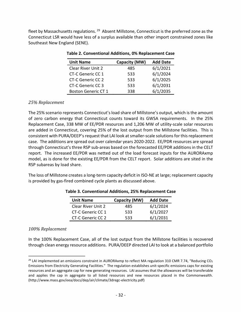
fleet by Massachusetts regulations. 29 Absent Millstone, Connecticut is the preferred zone as the Connecticut LSR would have less of a surplus available than other import constrained zones like Southeast New England (SENE).
Table 2. Conventional Additions, 0% Replacement Case
Unit Name Capacity (MW) Add Date Clear River Unit 2 485 6/1/2021 CT-C Generic CC 1 533 6/1/2024 CT-C Generic CC 2 533 6/1/2025 CT-C Generic CC 3 533 6/1/2031 Boston Generic CT 1 338 6/1/2035
25% Replacement
The 25% scenario represents Connecticut’s load share of Millstone’s output, which is the amount of zero carbon energy that Connecticut counts toward its GWSA requirements. In the 25% Replacement Case, 338 MW of EE/PDR resources and 1,206 MW of utility-scale solar resources are added in Connecticut, covering 25% of the lost output from the Millstone facilities. This is consistent with PURA/DEEP’s request that LAI look at smaller-scale solutions for this replacement case. The additions are spread out over calendar years 2020-2022. EE/PDR resources are spread through Connecticut’s three RSP sub-areas based on the forecasted EE/PDR additions in the CELT report. The increased EE/PDR was netted out of the load forecast inputs for the AURORAxmp model, as is done for the existing EE/PDR from the CELT report. Solar additions are sited in the RSP subareas by load share.
The loss of Millstone creates a long-term capacity deficit in ISO-NE at large; replacement capacity is provided by gas-fired combined cycle plants as discussed above.
Table 3. Conventional Additions, 25% Replacement Case
Unit Name Capacity (MW) Add Date Clear River Unit 2 485 6/1/2024 CT-C Generic CC 1 533 6/1/2027 CT-C Generic CC 2 533 6/1/2031
100% Replacement
In the 100% Replacement Case, all of the lost output from the Millstone facilities is recovered through clean energy resource additions. PURA/DEEP directed LAI to look at a balanced portfolio
29 LAI implemented an emissions constraint in AURORAxmp to reflect MA regulation 310 CMR 7.74, “Reducing CO2 Emissions from Electricity Generating Facilities.” The regulation establishes unit-specific emissions caps for existing resources and an aggregate cap for new generating resources. LAI assumes that the allowances will be transferable and applies the cap in aggregate to all listed resources and new resources placed in the Commonwealth. (http://www.mass.gov/eea/docs/dep/air/climate/3dregc-electricity.pdf)
- 32 -

approach with an appetite for large-scale solutions. Preference was given to local solutions, so no on-shore wind from Northern New England was included in the buildout.
Table 4. 100% Replacement Case Additions (MW by Year, Incremental)
Year 2020 2021 2022 2023 2024 Import Transmission 0.0 1000.0 0.0 0.0 0.0 Connecticut Utility-Scale Solar 804.0 804.0 804.0 0.0 0.0 EE/PDR 225.7 225.7 225.7 0.0 0.0 Off-Shore Wind 0.0 0.0 0.0 0.0 372.0
Import transmission is assumed to connect into the CT-Central RSP subarea. Import flows are expected to behave similarly to the existing HQ Phase II line, only scaled down to reflect lower line capacity. OSW is assumed to be connected to the Brayton Point substation (RI subarea) as an extension of the Massachusetts 83C procurement. EE/PDR and utility-scale solar are sited among the RSP subareas in the same proportions as used in the 25% Replacement Case. The capacity additions outlined above defer the need for new gas-fired capacity to 2035.
1.1.4 Results
Model Review
EPIS, AURORAxmp’s licensor, provides the model database that is the foundation for LAI’s forecasts. The EPIS default database is calibrated using a prior-year backcast in many installment updates. LAI also compared near-term forecast Market Heat Rates (MHRs) to recent history to ensure realistic results.
MHRs are calculated by dividing the power price by the appropriate marginal fuel (in this case, natural gas transported by Algonquin to New England, i.e., Algonquin Citygates). In ISO-NE, delivered natural gas prices are the single largest driver of wholesale energy prices. Even over the short run, forecasted power prices may not look similar to recent history due to changes in gas prices. However, the generating resource mix generally does not change significantly over the course of a few years. We can compare the average efficiency of the resource mix at different gas and power price using MHRs. We compare the average forecasted pool price MHRs to historical MassHub MHRs to evaluate whether LAI’s use of AURORAxmp is resulting in an accurate evaluation.
- 33 -

Figure 27. ISO-NE Average Monthly MHR comparison
The MHR comparison shows that the resource mix behaves the same way in the forecast as it has historically. MHRs peak in the summer, decline in the shoulder periods, and reach bottom in the winter. Elevated prices in the shoulder months can often be explained by nuclear outages that decrease the efficiency of the system mix, as less-efficient gas generators are called on more often. The forecast pattern and range is a good match with historical behavior.
Reference Case
All Aurora results are presented in 2017 real dollars. In the Reference Case we found that prices in the Connecticut-Central (CT-C) RSP subarea averaged around $40/MWh.
- 34 -

Figure 28. Annual Average Prices, Reference Case
Clean energy additions to the resource mix and decreasing net demand due to EE/PDR provide downward pressure on prices. Increasing RGGI emission allowance prices and net peak increases (despite EE/PDR) provide upward pressure on price. These factors generally offset each other, resulting in limited changes to MHRs. Given the limited changes in gas prices, there are limited changes to power prices.
Sensitivities
High/Low Gas Price Cases
The High/L Gas Price Cases only varied gas commodity prices and basis, and did not change the resource mix and other input assumptions.
- 35 -

Figure 29. Gas and Power Price Comparison
The power prices do not appear to have the same bandwidth as the gas prices -- the power price for the Low Gas Price Case has a higher MHR than the Reference Case. With a lower gas price, other dispatch costs such as variable O&M and RGGI allowance prices represent a larger portion of the resultant price. The converse happens in the High Gas Price Case; MHR in the High Gas Price Case is lower relative to the Reference Case as dispatch costs represent a smaller portion of resultant prices. In addition, oil becomes in merit far more often in the High Gas Price Case due to high winter prices. Non-gas dispatch during winter months also dampens the relationship between gas and power prices, as lower-priced coal and oil become the marginal resources more often.
High RE Development / EV Penetration Cases
The results did not reveal material sensitivity to RE or EV projects changing the resource mix and demand curve, respectively. The High RE Development projects were not sited in Connecticut locally, but still represent a large new source of price-taking RE for ISO-NE. It appears that the new RE resources do not force thermal units off of the margin relative to the Reference Case.
0
1
2
3
4
5
6
7
8
9
0
10
20
30
40
50
60
70
80
90
2018
2019
2020
2021
2022
2023
2024
2025
2026
2027
2028
2029
2030
2031
2032
2033
2034
2035
Gas
Pric
e (2
017
$/M
MBt
u)
Pow
er P
rice
(201
7 $/
MW
h)
Reference Case PowerLow Gas Price Case PowerHigh Gas Price Case PowerReference Case GasLow Gas Price Case GasHigh Ga Price Case Gas
- 36 -

Figure 30. Annual Average Power Prices – High RE Development / EV Penetration Cases
The EV Penetration Case yields higher off-peak pricing due to increased demand in off-peak hours, but the benefit is partially mitigated by reducing the amount of cycling capacity needed to meet on-peak demand. On-peak prices are reduced as more baseload plants can meet the flatter demand profile.
0
5
10
15
20
25
30
35
40
45
50
2018
2019
2020
2021
2022
2023
2024
2025
2026
2027
2028
2029
2030
2031
2032
2033
2034
2035
Pow
er P
rice
(201
7 $/
MW
h)
Reference CaseHigh RE Development CaseEV Penetration Case
- 37 -

Figure 31. Annual Average Power Prices – Reference / EV Penetration Cases
Figure 32. Hourly Average Baseline and EV Demand, ISO-NE 2030
0
10
20
30
40
50
60
2018
2019
2020
2021
2022
2023
2024
2025
2026
2027
2028
2029
2030
2031
2032
2033
2034
2035
Pow
er P
rice
(201
7 $/
MW
h)
Reference Case Off-PeakEV Penetration Case Off-PeakReference Case On-PeakEV Penetration Case On-Peak
- 38 -

Millstone Replacement Scenarios
There are three replacement scenarios: 0% (Do Nothing), 25% (Do Something) and 100% (Do Everything). The 25% and 100% Replacement Cases have been formulated to reasonably bracket the anticipated increased costs borne by Connecticut load under a Millstone light substitute GWSA strategy versus a Millstone heavy substitute GWSA strategy. There are both wholesale and retail price effects. Wholesale price effects relate to the change in energy prices in Connecticut and New England. Emission effects are separately stated and do not incorporate the shadow price of carbon in New England. Retail price effects relate to the additional program costs for clean energy technologies that supplant energy production from Millstone. Hence, the retail price effects address the increased distribution costs and/or non-bypassable distribution surcharges for the array of clean energy resources tested in the 25% and 100% Replacement Cases.
In this section, LAI reports the wholesale energy price effects as well as the change in carbon emissions. In Section 4.1, LAI defines the individual program costs, model approach and results with respect to retail price impacts.
0 % and 25% Replacement Cases
In the Millstone retirement cases, at this level of the analysis results focus on the impact of Millstone’s retirement on Connecticut ratepayers through energy price changes, and on Connecticut’s policy goals concerning CO2 emissions. Instead of examining simple average prices as in earlier sections, we examine load-weighted prices since loads are higher in higher-priced hours. A comparison of load-weighted energy prices in the Connecticut RSP subareas is shown below:
- 39 -

Figure 33. CT Average Annual Power Price Comparison, 0% and 25% Replacement Cases
Millstone’s postulated retirement results in a small increase in energy prices over the course of the Study Period for both cases, about 2%. Initially, the difference between the Reference and 25% Replacement Cases is about $2/MWh. As new merchant combined-cycle resources are added over the forecast period to meet reserve margin, the price difference narrows. In the 0% Replacement Case this change results in about a 2% increase in cost to load.
In the 25% Replacement Case costs to load actually decrease by about 5%. This is due to the avoided demand created by EE/PDR additions, which account for about 2.1 TWh, or about 7%, of Connecticut’s total energy demand. However, despite having a limited effect on the energy market, retirement of Millstone makes a significant impact on CO2 emissions.
0
5
10
15
20
25
30
35
40
45
50
2018
2019
2020
2021
2022
2023
2024
2025
2026
2027
2028
2029
2030
2031
2032
2033
2034
2035
Load
-Wei
ghte
d Po
wer
Pric
e (2
017
$/M
Wh)
Reference Case25% Replacement Case0% Replacement Case
- 40 -

Figure 34. Annual CO2Emissions, 0% and 25% Replacement Cases, Connecticut
For the 0% Replacement Case, the Millstone retirement results in about 53.4 million short tons of additional CO2 emissions from electric generators in Connecticut. Increased emissions in 2024-26 and 2031/32 are due to combined cycle additions that are needed to ensure that ISO-NE’s net ICR is met.
For the 25% Replacement Case, the Millstone retirement results in about 31.5 million short tons of additional CO2 emissions in Connecticut. Increased emissions in 2027/28 and 2031/32 are due to combined-cycle additions in Connecticut. The model caps CO2 emissions from large gas-fired units in Massachusetts to comply with regulations, so those units are already constrained and cannot increase output to offset the loss of Millstone. Most impacts to the thermal fleet are found in Connecticut and Rhode Island, since generators in Southern New England are closer to load than generators in Northern New England. Importantly, even though most of the increased emissions come from combined cycle additions, they are not the direct cause of the increased emissions. The cause of the increased emissions is the retirement of the Millstone units, which forces the existing gas fleet to work harder throughout the year. Having newer, more efficient combined cycle capacity available to meet the increased work burden on the conventional fleet actually reduces emissions relative to only increasing dispatch for the existing fleet. Retiring Millstone without making extensive clean energy replacements will make it challenging, to say the least, for Connecticut to reduce carbon emissions in the electric power sector. Simply put, Connecticut’s long-term goals set forth in the GWSA would likely be jeopardized unless an expensive technology substitution strategy is implemented.
0
2
4
6
8
10
12
2018
2019
2020
2021
2022
2023
2024
2025
2026
2027
2028
2029
2030
2031
2032
2033
2034
2035
Emis
sion
s (sh
ort t
ons)
Mill
ions
Reference Case25% Replacement Case0% Replacement Case
- 41 -
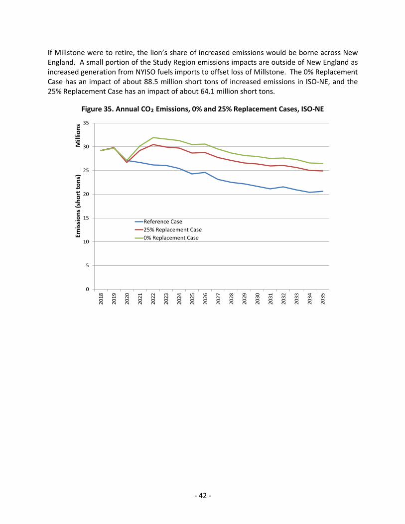
If Millstone were to retire, the lion’s share of increased emissions would be borne across New England. A small portion of the Study Region emissions impacts are outside of New England as increased generation from NYISO fuels imports to offset loss of Millstone. The 0% Replacement Case has an impact of about 88.5 million short tons of increased emissions in ISO-NE, and the 25% Replacement Case has an impact of about 64.1 million short tons.
Figure 35. Annual CO2 Emissions, 0% and 25% Replacement Cases, ISO-NE
0
5
10
15
20
25
30
35
2018
2019
2020
2021
2022
2023
2024
2025
2026
2027
2028
2029
2030
2031
2032
2033
2034
2035
Emis
sion
s (sh
ort t
ons)
Mill
ions
Reference Case25% Replacement Case0% Replacement Case
- 42 -

Figure 36. Annual Gas-Fired Generation, 0% and 25% Replacement Cases, ISO-NE
Increased emissions are explained by the increased dispatch of combined cycle resources to supplant lost Millstone output, including the new resources added to meet the Net ICR. In the 25% Replacement Case, combined cycle generation increases by about 25% over the planning period. More than one-half of the increased generation comes from new additions; the additions run at robust (around 75%) capacity factors.
The increase in combined cycle generation is similar for the 0% Replacement Case. Combined cycle generation increases by about 35%; combined cycle additions account for about 75% of the incremental generation.
Table 5. Annual Average Combined-Cycle Generation Comparison
Case
Total Generation
(TWh)
Capacity Factor
(%)
Existing Generation
(TWh)
Capacity Factor
(%)
New Generation
(TWh) Reference 40.5 33.4 40.5 33.4 - 25% Replacement 50.6 39.6 45.1 37.2 5.5 0% Replacement 54.5 41.0 44.2 36.5 10.3
A comparison of the generator gas burn found in the 25% Replacement Case and 0% Replacement Case relative to the Reference Case is illustrated in Figure 37. Figure 38 and Figure 39 show the geographic distribution of the incremental generator gas demand in each of the replacement cases.
0
10
20
30
40
50
60
70
2018
2019
2020
2021
2022
2023
2024
2025
2026
2027
2028
2029
2030
2031
2032
2033
2034
2035
Gas
-Fire
d G
ener
atio
n (T
Wh)
Reference Case25% Replacement Case0% Replacement Case
- 43 -

Figure 37. Incremental Generator Gas Demand, 0% and 25% Replacement Cases
Figure 38. Location of Incremental Generator Gas Demand, 25% Replacement Case
0
500
1,000
1,500
2,000
2,500
Jan-
18
Jan-
19
Jan-
20
Jan-
21
Jan-
22
Jan-
23
Jan-
24
Jan-
25
Jan-
26
Jan-
27
Jan-
28
Jan-
29
Jan-
30
Jan-
31
Jan-
32
Jan-
33
Jan-
34
Jan-
35
New
Eng
land
Gen
erat
or G
as D
eman
d (M
Dth/
d)Reference Case
25% Replacement Case
0% Replacement Case
-150
-100
-50
0
50
100
150
200
250
300
Jan-
18
Jan-
19
Jan-
20
Jan-
21
Jan-
22
Jan-
23
Jan-
24
Jan-
25
Jan-
26
Jan-
27
Jan-
28
Jan-
29
Jan-
30
Jan-
31
Jan-
32
Jan-
33
Jan-
34
Jan-
35
Incr
emen
tal D
eman
d Re
lativ
e to
Ref
eren
ce (
MD
th/d
)
Vermont RhodeIsland NewHampshire MassWestMassSoutheast MassCentral MaineSouth MaineCentralMaineBHE ConnSouthwest ConnCentral Boston
- 44 -

Figure 39. Location of Incremental Generator Gas Demand, 0% Replacement Case
LAI conducted an additional set of model runs first to develop gas basis calculations in GPCM reflecting the incremental generator gas demand in the 25% Replacement Case, and then to test the effects of the increased gas basis results in AURORAxmp. The incremental gas demand in New England yielded increased basis to New England delivery points. Figure 40 shows the change in average monthly delivered gas prices, represented by Algonquin Citygates.
- 45 -

Figure 40. Delivered Gas Price Forecast, 25% Replacement Case
This change in gas prices resulted in higher power prices, with an increase of about 6% relative to the Reference Case, but the demand decrease associated with EE/PDR meant that the basis adjusted case still ended up with a 1% decrease in cost to load in Connecticut.
$0
$5
$10
$15
$20
$25
Jan-
18
Jan-
19
Jan-
20
Jan-
21
Jan-
22
Jan-
23
Jan-
24
Jan-
25
Jan-
26
Jan-
27
Jan-
28
Jan-
29
Jan-
30
Jan-
31
Jan-
32
Jan-
33
Jan-
34
Jan-
35
AGT
CG D
eliv
ered
For
ecas
t (2
017
$/M
MBt
u)25% Replacement Case Reference Case
- 46 -

Figure 41. Connecticut Price Comparison, with Adjusted Basis Case Included
100% Replacement Case
With full replacement of the Millstone generation with clean energy sources, we found limited impacts on the resultant energy prices and emissions. Since Millstone is replaced with other price-taking resources, there are limited changes to the energy market outcomes, but the financial analysis will explain what capital investments would be made to fully replace Millstone output.
Market price changes were fairly limited, but expanded PDR development represented a 15% drop in demand over the Study Period for the Connecticut RSP subareas.
0
1
2
3
4
5
6
7
0
10
20
30
40
50
60
70
2018
2019
2020
2021
2022
2023
2024
2025
2026
2027
2028
2029
2030
2031
2032
2033
2034
2035
Gas
Pric
e (2
017
$/M
MBt
u)
Load
-Wei
ghte
d Po
wer
Pric
e (2
017
$/M
Wh)
Reference Case
25% Replacement Case
25% Replacement Case, Basis Adjusted
Algonquin, No Adjustment
Algonquin, Demand Adjusted
- 47 -
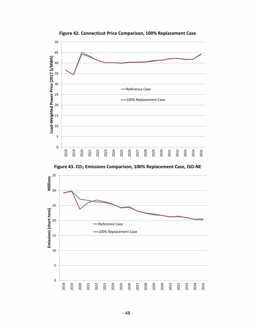
Figure 42. Connecticut Price Comparison, 100% Replacement Case
Figure 43. CO2 Emissions Comparison, 100% Replacement Case, ISO-NE
0
5
10
15
20
25
30
35
40
45
50
2018
2019
2020
2021
2022
2023
2024
2025
2026
2027
2028
2029
2030
2031
2032
2033
2034
2035
Load
-Wei
ghte
d Po
wer
Pric
e (2
017
$/M
Wh)
Reference Case
100% Replacement Case
0
5
10
15
20
25
30
35
2018
2019
2020
2021
2022
2023
2024
2025
2026
2027
2028
2029
2030
2031
2032
2033
2034
2035
Emis
sion
s (sh
ort t
ons)
Mill
ions
Reference Case
100% Replacement Case
- 48 -

Given the mitigating clean energy resources, we found similar emissions estimates for Reference and Full Replacement assumptions. The larger decrease in the 100% Replacement Case in 2020 represents the addition of PDR and utility-scale solar resources ahead of the Millstone retirement in May 2021. The full replacement resources keep Connecticut (and ISO-NE at large) on the same emissions trajectory as with Millstone operating, with limited differences in pricing and emissions. However, these results do not represent the costs of bringing the new resources online.
1.2 CAPACITY PRICE FORECAST
1.2.1 Millstone Historical FCA Revenues
Millstone units 2 and 3 have been able to rely on a steady revenue stream from the ISO-NE FCM since its first year of implementation in 2010. The first FCA was conducted in 2007 and since the FCA is conducted three years ahead of expected capacity delivery year, the 2010/2011 capacity commitment period (CCP) 30 was the first in which generators that cleared the FCA and had a CSO received capacity market payments. An analysis of FCA Obligations lists,31 which provide the monthly CSO for each unit that cleared the auction including both Millstone units, and the FCA resource clearing price for each CCP provides the revenues each Millstone unit has received through 2017 as well as what the units will receive through FCA 11 or May 31, 2021.32 The CSO for Millstone units 2 and 3 for each CCP is shown in Table 6 along with the resource clearing price from that FCA. Figure 44 provides the annual capacity revenues over each calendar year from June 1, 2010 through May 31, 2021.
Table 6. Millstone Unit CSOs & FCA Resource Clearing Prices
Capacity Commitment Period
Unit 2 CSO (MW)
Unit 3 CSO (MW)
FCA Resource Clearing Price ($/kW-Month)
2010/11 881 1235 $4.50 2011 /12 882 1235 $3.60 2012/13 880 1235 $2.95 2013/14 877 1225 $2.95 2014/15 877 1225 $3.21 2015/16 877 1225 $3.43 2016/17 876 1225 $3.15 2017/18 875 1225 $7.03 2018/19 875 1225 $9.55 2019/20 875 1225 $7.03 2020/21 872 1225 $5.30
30 Capacity commitment periods do not align with calendar years; a CCP begins on June 1 and runs through May 31 of the following year. 31 https://iso-ne.com/markets-operations/markets/forward-capacity-market/?document-type=FCA%20Results&file-type=XLS&file-type=XLSX&file-type=CSV 32 https://iso-ne.com/about/key-stats/markets#fcaresults
- 49 -

Figure 44. Millstone Unit-Level Annual Capacity Revenues
The introduction of the sloped demand curve with FCA #8 (CCP 2017/2018) saw a sharp increase in prices from what had been observed in the first seven FCAs – this can be seen clearly in the price spike in 2017 shown in Figure 44. During the period for which historical capacity and energy revenues can be analyzed, i.e., 2011 through 2016, capacity revenues accounted for an average of about 11% of Millstone’s total revenue each calendar year. Even in light of the observed increase in the resource clearing price with the introduction of the sloped demand curve with FCA #8, the Millstone units are expected to continue to make the lion’s share of their operating revenues through energy sales.33
1.2.2 Forward Capacity Market Structure34
The FCM was established in 2007 with the goal of ensuring reliability in the ISO-NE power system by conducting annual FCAs three years in advance of expected delivery to make certain there are enough generating (or demand-reducing) resources in the market, new or existing, to meet system-wide resource adequacy requirements.35
Beginning with FCA #9, ISO-NE adopted a two-part settlement system, Pay-for-Performance (P-f-P), which was designed to incentivize suppliers to ensure the reliability of their unit to perform
33 Capacity sales are expected to continue to provide Millstone with a steady revenue stream even if ISO-NE’s Competitive Auctions with Sponsored Resources (CASPR) proposal is adopted. 34https://www.iso-ne.com/static-assets/documents/2017/02/m20_forward-capacity-market_rev24_20170203.pdf 35 In addition to annual FCAs, there are reconfiguration and bilateral auctions that occur throughout the three years between the FCA and the CCP where CSOs can be shifted from one resource to another where necessary.
- 50 -

during periods of deficiency in operating reserves (i.e., capacity scarcity conditions or CSCs).36 The two-part settlement consists of both a Base Capacity Payment, which reflects the product of the resource’s CSO and the FCA resource clearing price, and a Capacity Performance Payment (CPP), a redistribution mechanism to reward resources that over-perform during CSCs with the funds collected from resources that underperformed and were penalized.
Base Capacity Payment
The Base Capacity Payment is based on the resource’s qualified summer capacity and the clearing price set in the FCA. ISO-NE determines the qualified capacity prior to the FCA; the qualified capacity as determined by ISO-NE is provided as a megawatt (MW) value that generally aligns with the CSO a resource receives if it clears the auction.37 LAI’s proprietary model for forecasting FCA resource clearing prices in dollars per kilowatt month ($/kW Month) provides the price that a generator can reasonably expect to receive for each Obligation Month in that CCP. The resource clearing price multiplied by the unit’s expected CSO represents the resource’s expected Base Capacity Payment for the Obligation Month.
Capacity Performance Payment
The CPP is based on resource performance during each CSC event and a Capacity Performance Score (CPS) that is calculated for each CSC that lasts from five minutes to an hour.38 Each CPS depends on both generator-specific parameters, for example, actual MW of generation provided at the time of the CSC and the resource’s CSO. It also depends on ISO-wide parameters, for example, the Balancing Ratio (BR)39 and the predetermined Performance Payment Rate (PPR) associated with that delivery year.40
36https://www.iso-ne.com/static-assets/documents/regulatory/ferc/filings/2014/jan/er14_1050_000_1_17_14_pay_for_performace_part_1.pdf 37 In addition to the site-specific data, the qualified capacity may be restricted by the capacity interconnection rights determined by ISO-NE in the context of the interconnection process. In some situations, ISO-NE may identify overlapping issues related to a group of new resources that are proposed in the vicinity of one another. 38 A stop-loss provision in the FCM rules limits the monthly and annual cumulative penalties. According to the FCM rules, capacity payments to intermittent resources are not subject to the availability adjustments: the performance measure for intermittent resources is already included in the determination of their summer and winter qualified capacity values. 39 The BR is calculated by dividing the load plus reserve requirement by the total ISO system-wide CSO of all available units. The BR provides the percentage of the resource’s CSO that must be supplied during the CSC to avoid a penalty payment. If a resource has a CSO of 100 MW and the BR associated with a CSC is 75% the resource will need to supply at least 75 MW or face paying a penalty payment. The CPP is the product of the CSC multiplied by the PPR for the commitment period. For each Obligation Month, the sum of all CPPs is either subtracted from the resource’s Base Capacity Payment if the net of all CPS’s is negative. It is added if the net of all CPS’s is positive. 40 For the three CCPs beginning June 1, 2018 and ending May 31, 2021. 21The CPPR is set at $2000/MWh. For the following three CCPs beginning June 1, 2021 and ending May 31, 2024, the CPPR is set at $3500/MWh. For the CCP beginning on June 1, 2024 and ending on May 31, 2025 and thereafter, the CPPR is set at $5455/MWh.
- 51 -

Proposed Market Structure Changes
ISO-NE’s CASPR proposal41 seeks to establish a two-tier capacity market that accommodates the entry of subsidized resources and the exit of unsubsidized existing resources from the capacity market. Should the CASPR proposal be accepted, thereby changing the FCM market structure, a different approach to forecasting FCA prices would be warranted. However, at this time, CASPR is evolving and has therefore not been considered in LAI’s modeling effort related to Executive Order 59.
1.2.3 LAI FCA Resource Clearing Price Forecast Methodology
Base Resource Clearing Price
LAI uses a proprietary model developed in-house to forecast base resource clearing prices in ISO-NE’s annual FCA, held three years in advance of expected capacity delivery, based on projections of demand curve parameters from ISO-NE and LAI’s projected resource balance. The capacity price forecast reflects long-term clearing prices in New England, but captures incumbent generator bidder behavior also demonstrated in PJM.42 LAI’s in-house model of the FCM captures ISO-NE’s two-part settlement system for providing capacity revenues by forecasting an FCA resource clearing price and producing an analysis of expected unit performance during scarcity hours.
Theoretically, the Net Cost of New Entry (Net CONE) is the expected operating margin a new-build resource would need to earn in capacity revenue in its first year after accounting for energy and ancillary services revenues to make it economically viable. Net CONE values are established prior to each FCA and used to determine demand curve parameters. In both ISO-NE and PJM, however, a significant gap between resource clearing prices and the administratively pre-determined Net CONE has been observed in nearly every FCA and BRA43 conducted, and new resources have cleared at prices below net CONE.
LAI developed a model to estimate the FCA resource clearing price based on the projected FCA demand curve parameters, technology progress, and an adjustment factor. The statistical model utilizes historical bidder dynamics in both PJM and ISO-NE and the demand-supply ratio (DSR) as a measure of market tightness as the foundation for the statistical model. LAI’s statistical model was estimated using the load-weighted resource clearing prices from previously conducted PJM BRAs and the DSR in each BRA year calculated using the RTO reliability requirement and the reported summer capacity.44 The relationship between the clearing price and its predictor, the
41 https://www.iso-ne.com/static-assets/documents/2017/04/caspr_discussion_paper_april_14_2017.pdf 42 In FCA #9, ISO-NE replaced the vertical demand curve structure used previously with a sloped demand curve, thus rendering prior auction results of no relevance for predictive purposes. Normative price curve analysis therefore requires technical analysis of incumbent generator bidder dynamics in PJM, which has historically employed a similar sloped demand curve to set capacity prices. The demand curve in NYISO is of limited relevance. 43 The BRA is PJM’s administrative construct for procuring capacity. 44 The model covers BRAs conducted starting with the 2010/2011 delivery year through the 2019/2020 delivery year.
- 52 -

DSR, is statistically significant and positive, indicating that an increase in the DSR (i.e., a smaller surplus or projected deficit of capacity in the market) will result in an increase in the resource clearing price.45
The historical DSR is the calculated ratio of the peak load plus the target reserve margin – the ICR – to the qualified summer capacity in that delivery year. The forecasted DSR is the calculated ratio of the ICR, or the 2017 CELT 50/50 peak load net PV for the calendar year plus a target reserve margin of 14.3%46 applied to LAI’s forecasted qualified summer capacity based on generator attrition, renewable resource buildout, and PDR/EE growth. Since the model foundation is based on historical PJM BRA results, in which a less tight market has resulted in clearing prices lower than those observed in ISO-NE’s FCA, an adjustment factor was applied to the model to calibrate the data to clearing prices observed in ISO-NE since the introduction of the sloped demand curve.
The output from the statistical model was applied to the projected DSR for each case to predict an FCA resource clearing price ($/kW-Month) for each CCP from FCA #13 (2021/2022) through FCA 27 (2035/2036).
P-f-P Risk Premium
LAI conducted an analysis of a potential increase (or decrease) to FCA resource clearing prices resulting from the two remaining step increases in the PPR from $2,000/MWh to $3,500/MWh with FCA #12 (2021/2022) and finally to $5,455/MWh with FCA #15 (2024/25). There are two parameters that change with each CSC: the BR47, which is a system-wide parameter specific to each event, and a resource’s actual generation, which is unit- and event-specific.
FCA #11 was conducted with the PPR of $2,000/MWh in place. Therefore it is assumed that generators built a risk premium into their bids in FCA #11 based on that penalty rate. LAI made assumptions about the number of expected CSCs, the system-wide BR, and the expected actual generation for a unit that resembles those used in ISO-NE’s CONE study to calculate expected CPPs for FCA #12 and FCA #15. We assumed nine CSCs annually,48 a system-wide BR of 64%,49 and actual generation of the unit equal to the expected CSO derated by two times the EFORd of
45 To calibrate the model output to ISO-NE, in which observed resource clearing prices have been higher than in PJM, the average clearing price from the three most recent forward auctions for each RTO was calculated and weighted equally and then applied to the model in place of the estimated constant term. 46 ISO-NE System Planning. 2015 Regional System Plan. November 5, 2015. p. 47. 47 BR = Total System Load + Reserve Requirement / Total Available System-wide CSO 48 The expected number of CSCs was taken from the ISO-NE’s Estimated Hours of System Operating Reserve Deficiency – Final Results (Capacity Commitment Period 2020-2021 presentation for the 50/50 forecasted scarcity hours at the ICR + 400 level of cleared capacity. 49 The BR was calculated by taking the average of all Reserve Constraint Penalty Factors from 2007 through 2016 based on ISO-NE’s Reserve Constraint Penalty Factor Activation Data.
- 53 -
7.5% for a combustion turbine.50 In order to determine what additional risk premium would be added to bids on top of what is assumed to have been added to bids in FCA #11, the change from FCA #11 expected CPP to FCA #12 and from FCA #11 to FCA #15 was calculated. Based on the aforementioned parameters, LAI determined that generator tolerance for the incremental risk associated with different performance rates was negligible, i.e., an incremental increase of $0.07/kW-Month for FCA #12 and an additional $0.09/kW-Month for FCA #15. Hence, no adjustment to the Base Capacity Price forecast was deemed necessary.51
1.2.4 FCA Model Results
Reference Case
LAI forecasted FCA prices for the Reference Case using our in-house proprietary model based on LAI’s forecasted resource mix and demand curve parameters. The resource mix builds on the assumptions described in the resource additions and resource retirements sections of this report.52 LAI reviewed the LSRs for zones that could price separate, including Boston, Connecticut, and SENE, and determined there would be no expected price separation in future FCAs as all zones had at least a 1,500 MW surplus compared to its LSR. Demand values used to calculate LSRs were based on the 2017 CELT report peak load net PV.
The LAI model was applied to the DSR based on the assumptions outlined above. The resulting prices are shown in Figure 45. FCA prices forecasted by LAI begin with the 2021 capacity year and end with the study period in 2035.53 Despite some resource retirements, generally slow load growth over the forecast period and a surplus of capacity in the market produce a fairly steady, slowly increasing FCA price forecast. Age-based retirements in 2024 and 2031 increase market tightness slightly, causing minor upward pressure on the FCA price in those years. FCA prices do not reach Net CONE, which was projected based on inflation, assumptions on technological progress, and expected net energy margins for the CONE unit from ISO-NE’s FCA #12 CONE study and is shown in Figure 45, which is reasonable based on historical capacity market dynamics.
50 The EFORd was calculated as the five-year average for the technology type based on historical ISO-NE ICR values reports for FCA 9, FCA 10, and FCA 11. 51 More rigorous testing of P-f-P parameters affecting incumbent generator risk exposure may be warranted as part of CT DEEP’s 2018 Integrated Resource Plan. 52 Resources were derated to an FCA qualified capacity level for use in calculating the DSR based on the rules ISO-NE has established for each technology type for FCA-qualified resources. Conventional resources were derated by subtracting one times the forced outage rate from resource net capability. Renewable resources were derated by their expected generation during summer and winter reliability hours. Summer reliability hours are those ending 1400 through 1800. Winter reliability hours are those ending 1800 through 1900. 53 As a three-year forward market, FCAs have been conducted covering the period through May 31, 2021.
- 54 -

Figure 45. Reference Case ISO-NE Net CONE & FCA Prices (nominal $)
Low & High Gas Price Cases
For both the Low and High Gas Price Cases, the resource mix remained unchanged from the Reference Case. With the DSR as the foundation of LAI’s forecast of FCA clearing prices remaining constant across the Reference, High Gas Price and Low Gas Price Cases, FCA clearing prices reflect only small changes in net energy margins based on LAI’s wholesale energy market forecast.
Capacity payments are often considered the necessary missing money a new conventional unit would need to cover its net going forward costs after accounting for expected revenues from energy and ancillary services sales. To determine the effects of the different gas price forecasts on expected required capacity revenues to cover net going forward costs, LAI analyzed divergences from the in the forecasted market heat rate in the Reference Case for both the High and Low Gas Price Cases. Results extracted from AURORAxmp modeling were used to calculate the market heat rate for the Reference, High Gas Price and Low Gas Price Cases. The $3.31/kW-Month in 2021 dollar revenue offset from the ISO-NE CONE and ORTP Analysis54 was projected out assuming a 2% inflation rate and used as the starting point to which the percentage change in market heat rate was applied to arrive at the expected change in capacity prices required by a new entrant to cover net going forward costs in the event of high or low gas prices. Figure 46
54 https://www.iso-ne.com/static-assets/documents/2017/01/cone_and_ortp_updates.pdf
0
2
4
6
8
10
12
14
2017
2018
2019
2020
2021
2022
2023
2024
2025
2026
2027
2028
2029
2030
2031
2032
2033
2034
2035
Pric
e ($
/kW
-Mon
th)
Capacity Year Beginning June 1
Net CONE Resource Clearing Price
- 55 -

shows the difference in capacity prices for the High and Low Gas Price Cases relative to the Reference Case.
Figure 46. Reference, High Gas Price, and Low Gas Price Case FCA Prices (nominal $)
Millstone Retirement Replacement Cases
LAI produced FCA prices for the three Millstone retirement and postulated replacement cases: 0% replacement, 25% replacement, and 100% replacement. The FCA prices for each of the replacement cases build on the assumptions surrounding the resource mix outlined in the 0% Replacement Case, 25% Replacement Case, and 100% Replacement Case sections of this report. Figure 47 shows the projected Net CONE and forecasted FCA prices for the Reference Case and each of the Millstone replacement cases. An initial increase in FCA prices is observed immediately with FCA #12 due to the retirement of both Millstone units, which combine for just over 2,000 MW of FCA qualified capacity.
Divergences from the Reference Case FCA prices in three replacement cases are driven primarily by the timing and technology of replacement generation. FCA prices in all Millstone replacement cases converge with the Reference Case toward study period end due to the build out of conventional and renewable resources becoming nearly equal across the cases relative to the projected demand, which is not case dependent.
0
2
4
6
8
10
1220
17
2018
2019
2020
2021
2022
2023
2024
2025
2026
2027
2028
2029
2030
2031
2032
2033
2034
2035
FCA
Pric
e ($
/kW
-Mon
th)
Capacity Year Beginning June 1
Low Gas Price CaseHigh Gas Price CaseReference Case
- 56 -

Figure 47. Reference and Millstone Replacement Cases FCA Prices (nominal $)
0% Replacement Case
The initial spike in FCA prices is highest in the 0% Replacement Case, though it is insignificantly higher than the 25% Replacement Case due to the immediate need for gas-fired resources in the absence of clean replacement resources. In the 0% Replacement Case, it is assumed that a combined cycle unit is needed to meet reliability requirements as soon as FCA #12. The FCA price drops below the price in the 25% Replacement Case in 2025 and 2026 because the need for additional combined cycle units in both 2024 and 2025 to meet reliability requirements causes a small, short-term surplus of MW of capacity relative to the capacity in the 25% Replacement Case. Prices remain nearly constant in real terms beyond 2027.
25% Replacement Case
There is an initial spike in FCA prices compared to Reference Case due to the Millstone retirements not being replaced by 25% clean energy resources in 2021 but rather over a three-year period. The FCA price in 2027 drops below the 0% Replacement Case as a combined cycle is added to meet reliability requirements. FCA prices in the 25% Replacement Case converge with the Reference Case and 100% Replacement Case in 2027.
100% Replacement Case
FCA prices are closest to Reference Case in the 100% Replacement Case due to the early replacement of Millstone capacity needed to meet ISO system-wide reliability targets met with
0
2
4
6
8
10
12
14
2017
2018
2019
2020
2021
2022
2023
2024
2025
2026
2027
2028
2029
2030
2031
2032
2033
2034
2035
FCA
Pric
e ($
/kW
-Mon
th)
Capacity Year Beginning June 1
Net CONE0% Replacement Case25% Replacement Case100% Replacement CaseReference Case
- 57 -

clean energy resources between 2021 and 2024. The postulated 1,000 MW HVDC line is assumed to be a capacity resource. Since the HVDC line is needed to meet reliability targets, omitting it from the capacity supply mix would result in short-term upward pressure on capacity prices that would otherwise be alleviated by traditional entry to meet the net ICR.
1.2.5 Millstone P-f-P Penalty Exposure
Millstone Maximum Penalty Exposure
In order to limit the total financial loss a resource with a CSO can sustain as a result of underperformance during CSCs with both per month and over the entire twelve-month capacity commitment period, Monthly55 and Annual Stop-Loss provisions were adopted as a part of the P-f-P Initiative. The capacity stop-loss mechanism is defined in ISO-NE Market Rule 1 (MR 1) Section 13.7.3. The Stop-Loss provisions represent the maximum possible downside for a resource with a CSO rather than the realistic penalty exposure risk.56
Based on the Stop-Loss provisions in MR 1 related to CPPs, the maximum penalty exposure for Millstone units 2 and 3 for years where relevant FCA parameters are available can be calculated. The following calculation example uses the parameters from the most recent FCA conducted for the capacity commitment period 2020/2021, FCA 11. Millstone unit 2 has a monthly CSO of 872.26 MW for each Obligation Month in the period, and Millstone unit 3 has a monthly CSO of 1225 MW for each Obligation Month in the period.57 The Starting Price for FCA 11 was $18.63/kW Month and the resource clearing price, cleared in round 5 of the auction, was $5.30/kW Month.58
Table 3 provides the Annual Stop-Loss for each Millstone Unit based on the FCA #11 parameters and the equation provided by MR 1 Section 13 III.13.7.2 (a). The Annual Stop-Loss limits the amount of losses possible on a monthly basis once the annual limit is met.
55 The Monthly Stop-Loss on CPP applies only in situations where the sum of all CPP in an Obligation Month is negative. Per MR 1 III.13.7.3.1, “the amount subtracted from the resource’s Capacity Base Payment for the Obligation Month will be limited to an amount equal to the product of the applicable FCA Starting Price multiplied by the resource’s CSO for the Obligation Month.” The Monthly Stop-Loss on CPPs thus does not limit the penalties to a zeroing out of the Base Capacity Payment for the Obligation Month. This is because the FCA starting price is equal to 1.6 times Net CONE. 56 Per MR 1, Section 13 III.13.7.2, the Annual Stop-Loss provision limits the amount of annual losses such that the annual Stop-Loss limit for the Millstone units is not equal to twelve times the Monthly Stop-Loss limit for each unit. Calculating the Annual Stop-Loss for each Millstone unit provides the maximum possible loss each unit could face due to non-performance. It represents a theoretical limit. 57 FCA 11 Obligations List, ISO-NE. 58 https://www.iso-ne.com/static-assets/documents/2017/02/fca_11_result_report.pdf
- 58 -

Table 7. Millstone Units Annual Stop-Loss
Unit CSO
(MW) FCAsp
($/kW-mo) FCAcp
($/kW-mo) Annual Stop-Loss Limit
($) Millstone 2 872.26 $18.63 $5.30 ($90,317,955) Millstone 3 1225 $18.63 $5.30 ($126,842,625)
Millstone’s Expected Penalty Exposure
While the previous section presents the maximum possible penalty exposure the Millstone units could face under P-f-p and the Stop-Loss provisions adopted with it, it does not represent the realistic penalty exposure for the units. It represents an absolute upper bound. As Nuclear Engineering International pointed out in an article published in early 2016, the impact of P-f-P on nuclear resources may actually be a net positive.59 Additionally, Millstone Unit 2 had been considered more likely to be exposed to the risk of non-performance during CSCs after it was forced out for 12 days in 2012 due to water temperature in the Long Island Sound exceeding 75 degrees. On April 18, 2014, the NRC granted a license amendment allowing Millstone Unit 2 to operate with a heat sink water temperature of up to 80 degrees.60 No forced outages have occurred for Millstone Unit 2 since the approval of that amendment.
Since P-f-P begins with the 2018/2019 capacity commitment period and no historical data has been recorded as a result, analyzing the ISO-NE Reserve Constraint Penalty Factor Activation Data for the last ten years provides a proxy for when a CSC may have been called and what the average duration of such events has been. There have been 191 occurrences of operating reserve deficiency between January 2007 and August 2016. Most of the events have occurred in February or the summer months as shown in Figure 48 along with the average BR for historical events in that month.
59 Angwin, Merideth. “Pay for Performance’ and the US grid.” Nuclear Engineering International. February, 2016. 60 http://www.ct.gov/deep/lib/deep/radiation/neac_2014_annual_report.pdf
- 59 -

Figure 48. Historical Reserve Deficiency Event Frequency and Balancing Ratio
Millstone will not be exposed to P-f-P risks when down for refueling in April or October. When a resource is scheduled out for maintenance and refueling, it is not considered available. Therefore no capacity is available under P-f-P. As shown in Figure 48, the months in which the Millstone units refuel have experienced the lowest frequency of scarcity conditions with low BRs. Based on Millstone’s commendable record of performance and availability, in LAI’s opinion, it is unlikely that either Millstone unit would come close to meeting the Monthly Stop-Loss provision based on the historical generation patterns and the historical average BR in each month.61
61 If, say, Millstone Unit 2 were to experience a full forced outage (i.e., supplied 0 MW of actual generation) in February with a BR of 56%, it would take 17 CSCs before the unit would reach the Monthly Stop-Loss provision. Likewise, if Millstone Unit 2 were to experience a full forced outage in July with a BR of 85%, it would take 11 CSC events to reach the Monthly Stop-Loss. The historical data show a maximum of 12 operating reserve deficiencies in one month, February 2008 and May 2010. Hence, it is highly unlikely that Millstone could reach the Monthly Stop-Loss. The likelihood of Millstone triggering the Annual Stop-Loss is remote.
- 60 -

2 MILLSTONE OPERATING EXPENSE FORECAST
During the course of this due diligence, Dominion was asked by DEEP/PURA to provide unit-specific cost and operating information to facilitate the financial assessment of Millstone’s future. In various communications to DEEP / PURA, Dominion indicated its unwillingness to provide confidential information to DEEP / PURA or to LAI. 62 Efforts to obtain such information under a non-disclosure agreement between Dominion and LAI were unsuccessful. Therefore, to meet the study goals and objectives, LAI resorted to public sources of information in order to develop reasonable indicators of Millstone’s operating costs.
There are four main categories of expenses that LAI has forecasted for Millstone:
• Fuel cost
• O&M cost
• Capital Expenditures
• Non-Operating Expenses (property taxes, sales and use tax, insurance, and General & Administrative loading factor)
2.1 MILLSTONE PLANT DESCRIPTION
The Millstone Station is located in Waterford and consists of three units. Millstone Unit 1 was a 2011 MWt (thermal rating) 652 MW (electrical rating) Boiling Water Reactor (BWR). It commenced operation in 1970 and ceased operating in 1995. Three years later, the NRC was notified that Millstone 1 had permanently ceased operation and fuel removed from the reactor vessel. The plant is now in SAFSTOR until 2048 with the spent fuel in a storage pool.63
Millstone Unit 2 was constructed by Bechtel using a Combustion Engineering two-loop Pressurized Water Reactor (PWR) design. It received its original NRC Operating License in 1975 that was renewed in 2005 and will now expire on July 31, 2035. Millstone Unit 2 received NRC approval for a 5% stretch uprate in 1979 and is now licensed to operate at 2,700 MWt. 64
62 See letter from Paul D. Koonce, Executive Vice President & President of Dominion Power Generation Group to Commissioner Rob Klee and Chairwoman Katie Dykes, September 19, 2017. 63 SAFSTOR is one of three decommissioning methods accepted by the NRC. Under SAFSTOR, also referred to as deferred dismantling, a nuclear facility is maintained and monitored while the radioactivity decays until the plant is dismantled and the property decontaminated and released. Spent nuclear fuel rods are encased in special casks and stored on a pad. The other two methods are DECON, immediate dismantling and decontamination so the property can be released, and ENTOMB in which radioactive contaminants are permanently encased on site in structurally sound material. No nuclear plants have requested the ENTOMB option. 64 The NRC has three categories of uprates. Stretch uprates are within the design capacity of a plant and involve changes to instrumentation setpoints, but not major modifications. NRC Operating Licenses determine the reactor’s maximum thermal energy output, expressed as MWt. The other two options are Measurement Uncertainty Recapture Power uprates of less than 2% achieved by installing improved instruments to measure feedwater and other variables more precisely, and Extended Power uprates of up to 20% that require significant modifications and/or investments.
- 61 -

Millstone Unit 2 has a nameplate rating of 910 MW and a Summer Claimed Capacity rating of 857 MW per ISO-NE’s 2017 CELT Report.
Millstone Unit 3 was constructed by Stone & Webster using a Westinghouse four-loop PWR design and a GE turbine-generator. It received its original NRC Operating License in 1986 that was renewed in 2005 and will now expire on November 25, 2045. Millstone Unit 3 received NRC approval for a 7% stretch uprate in 2008 and is now licensed to operate at 3,650 MWt. Millstone Unit 3 has a nameplate rating of 1,253 MW with a Summer Claimed Capacity rating of 1,255 MW per ISO-NE’s 2017 CELT Report.
Dominion purchased 100% of Millstone Unit 2 and 93.5% of Millstone Unit 3 from Northeast Utilities. The sale closed on March 31, 2001. The other joint owners of Millstone Unit 3 are Green Mountain Power with 1.7% and Massachusetts Municipal Wholesale Electric Company with 4.8%. 65 Dominion operates Millstone Unit 3 and is authorized to act as agent for the joint owners. The reactor differences between Units 2 and 3 have some variation in components and Dominion operators have separate NRC licenses for each unit. LAI confirmed with NRC there are no other approved or pending upgrades for Millstone Units 2 and 3.
2.2 HISTORICAL FUEL AND O&M EXPENSE DATA
2.2.1 Millstone Role in ISO-NE
Millstone has been the energy backbone of Connecticut’s resource portfolio. Millstone’s annual energy production has been about 16,000 GWh. Connecticut’s net load and net peak load have been flat or declining for several years. According to ISO-NE, Connecticut’s net load was 30,420 GWh and net peak load was 6,569 MW in 2016. Hence, Millstone has produced on average roughly one-half of total energy used in Connecticut and represents roughly one-third of the total installed capacity in the Connecticut load zone.
Since Dominion’s acquisition of Millstone in 2001, Millstone has been a reliable baseload generation resource. According to NEI, Millstone Unit 2 operated at a 97.7% capacity factor in 2016 and an average 89.6% over the three year period, 2014-2016. Millstone Unit 3 operated at an 85.2% capacity factor in 2016 and an average 90.4% capacity factor over the same three year period. Both units have occasionally tripped off line over the past few years. The NRC presented its most 2016 Annual Assessment to the Connecticut Nuclear Energy Advisory Council.66
As dependence on natural gas for energy production has heightened and both coal and other nuclear plants in New England have retired, Millstone has provided ISO-NE with fuel diversity benefits, particularly in the heating season when unit availability is high and pipeline
65 Central Vermont Public Service originally held a 1.7% ownership share in Millstone Unit 3 that was transferred to Green Mountain Power when the companies merged in 2012. 66 The NRC found that “the performance at Millstone Units 2 and 3 during the most recent quarter was within the Licensee Response Column, the highest performance category of the NRC’s Reactor Oversight Process Action Matrix in Inspection Manual Chapter 0305, Operating Reactor Assessment Program, because all inspection findings had very low safety significance and all PIs were within the expected range.”
- 62 -

deliverability constraints often arise, thereby limiting the availability of natural gas to the fleet of combined cycle plants and peakers. This fuel diversity benefit may become more valuable going forward as ISO-NE’s Winter Reliability Program ends in 2018.
2.2.2 Data Sources
There is no recent and accurate Millstone-specific expense data in the public domain.67 Previously, Northeast Utilities filed annual FERC Form 1 reports, but Dominion is not obligated to file these reports since purchasing Millstone in 2001 since only regulated utilities must file FERC Form 1s. Given the age of the data and change in ownership, LAI chose not to rely on Millstone Form 1 cost data available from Northeast Utilities. Therefore LAI reviewed two current sources of nuclear operating expense data to estimate Millstone’s fuel and O&M expenses: first, annual average expenses complied by NEI for the entire US nuclear fleet; and, second, recent plant-specific FERC Form 1 data for nuclear plants owned by regulated utilities. This FERC data includes the Surry and North Anna plants, regulated nuclear assets owned and operated by VEPCO, a Dominion company.68
Reliance on NEI and FERC Form 1 data has both advantages and disadvantages. NEI’s “Nuclear Costs in Context” is an up-to-date and unassailable industry data source covering nuclear plants throughout the U.S. The most recent NEI report reflects 2016 costs. NEI separates operating cost into three categories: fuel expense, O&M expense, and CapEx. NEI also differentiates cost data into single versus multi-unit plants as well as single plant versus multiple plants ownership. There are limitations associated with NEI data, however. NEI does not provide plant-specific data, does not differentiate between technology type, i.e., BWR versus PWR, and does not provide any data covering non-operating expenses.
LAI believes it is reasonable to rely on FERC Form 1 data for Millstone’s fuel and O&M expenses. Like reliance on NEI, there are also limitations, however. Annual Form 1 data are unit-specific in regard to nuclear fuel and O&M expenses, but only for the cohort group of nuclear power plants owned by regulated utilities. The Form 1 data do not include unit-specific CapEx or non-operating expenses. The FERC Form 1 data include VEPCO’s Surry and North Anna plants that have twin PWRs, as does Millstone.69 In light of the strength of Dominion’s management and similar technology, LAI believes that their underlying cost structure and performance statistics are substantially similar to Millstone. Absent information disclosure from Dominion, actual cost differences between the Dominion regulated fleet in Virginia and the unregulated nuclear units in Connecticut cannot be known with certainty.
Table 8 below, taken from NEI’s “Nuclear Costs in Context,” presents 2016 summary data for virtually the entire US nuclear fleet. The NEI data indicate that multi-unit plant sites (as is
67 Dominion does not provide this data, nor do the other owners of Millstone Unit 3, Green Mountain Power and MMWEC. 68 NEI published “Nuclear Costs in Context” in August, 2017, which was based on confidential plant data collected by the Energy Utility Cost Group (EUCG). 69 VEPCO owns 100% of Surry and 88.4% of North Anna.
- 63 -

Millstone) have lower costs than the industry average, as do fleet owners (such as Dominion). Since retirement of Dominion’s single Kewaunee unit in Wisconsin, Dominion now has three nuclear plant sites: Surry, North Anna and Millstone. Each site has two PWR units.
Table 8. 2016 NEI Nuclear Plant Cost Summary ($/MWh)70
Category
Number of Plants/
Sites Fuel Capital Operating
Total (Fuel +
Operating)
Total (Fuel + Capital + Operating)
All U.S. 60 6.76 6.74 20.43 27.19 33.93 Plant Size
Single Unit 25 6.77 8.67 25.95 32.72 41.39 Multi-Unit 35 6.75 6.15 18.73 25.48 31.63
Operator Single 12 7.18 8.19 21.20 28.38 36.57 Fleet 48 6.63 6.32 20.21 26.84 33.16
2.2.3 Basis for Applying Surry and North Anna FERC Form 1 Fuel and O&M Expense Data to Millstone
As LAI understands it, Dominion’s PWRs are sufficiently comparable to permit sharing of lessons learned, best practices, and economies of scale by Dominion in its regulated and unregulated nuclear operations. We have made the reasonable assumption that Millstone has a common management team rather than separable teams for the individual units. We have also assumed that (i) all departments (other than licensed operators) are common across the station including security, maintenance, engineering, chemistry, health physics, work management, site services, supply chain, IT, emergency response, training, corrective actions, and administrative groups; (ii) all station processes (training, work management, engineering, corrective actions, business, modifications, emergency response, etc.) and administrative procedures are common; and (iii) Dominion’s fleet processes and procedures are common to all Dominion nuclear units regardless of cost of service regulation.
VEPCO’s North Anna and Surry each have two units. North Anna Unit 1 has an installed capacity of 839 MW and was placed in service in 1972. North Anna Unit 2 has an installed capacity of 799 MW and was placed in service in 1973. According to Dominion’s 2016 10-K, the net summer capacity of Dominion’s share of North Anna is 1,672 MW, corresponding to a total nameplate capacity of 1,891 MW. The NRC extended the operating licenses for the North Anna units for twenty years to 2038 and 2040, respectively. The Surry units went on-line in 1972 and 1973, respectively. According to Dominion’s 2016 Form 10-K, the net summer capacity of Surry is 1,676 MW. The NRC extended the operating licenses for the Surry units for 20 years to 2032 and 2033.
The North Anna, Surry and Millstone nuclear units all use PWR technology, thereby supporting the basis to apply cost data from the VEPCO fleet in forecasting Millstone’s fuel expenses,
70 Source: Electric Utility Cost Group (EUCG)
- 64 -

operating expenses, and CapEx. The common technology also facilitates the sharing of lessons learned to support high unit availability and efficient cost management. We believe that the common PWR design facilitates cost savings in engineering, operations, and maintenance. As we understand it, Dominion shares lessons learned and best practices across the nuclear fleet. As repairs, improvements, and enhancements are made on one unit, Dominion has the opportunity to draw from experience and implement the best solutions among the other units. Trained crews – both full time Dominion employees and contract labor – can be mobilized among the fleet for specialized maintenance activities. From a technology standpoint, LAI recognizes that Dominion’s nuclear units have two-loop, three-loop, and four-loop PWR designs, but that the number of loops is secondary in nature relative to the more fundamental technology considerations associated with BWRs versus PWRs. Hence, we assumed that the number of loops does not significantly affect operating costs or unit availability in terms of capacity factor, refueling requirements, or operating regime. For these reasons and others, LAI assumes that the underlying cost data associated with operating the North Anna and Surry stations in Virginia is reasonably representative of Dominion’s experience operating Millstone.
We have made the simplifying assumption that Millstone personnel routinely conduct activities on both units. Refueling and maintenance outages are scheduled, planned, coordinated and executed to maximize the use of all station personnel using a common framework. Historic refueling outages coordinated with ISO-NE show that the operating cycles for both units are approximately 18 months and scheduled to occur in spring and fall when potential system-wide scarcity events are unlikely. Outages are scheduled so that only one unit is off-line at a time and station resources can be allocated to the unit undergoing maintenance and refueling. We assume that Millstone’s budget is allocated to the station and subsequently to each department – common across both units. We assume that there is not separate financial management accountability for each unit and that when major capital modifications are made, Dominion endeavors to install similar equipment on both units. For example, the variable frequency drives for the main circulating water systems utilize similar equipment at both units which optimizes parts and maintenance costs.
In weighing the pros and cons of basing Millstone’s fuel and O&M expenses on NEI data or Dominion’s FERC Form 1 data for North Anna and Surry, we recognize that nuclear plant owners typically share lessons learned and best practices among assets. In LAI’s view, nuclear plant owners share lessons learned regardless of technology type and market risk exposure. Fleet owners also have bargaining power when it comes to purchasing fuel, consumables, services, and equipment. These benefits are demonstrated by the fact that the fuel and O&M expenses for North Anna and Surry are remarkably similar and materially lower than the industry average as illustrated in Table 9. Dominion’s fleet of six operating nuclear units provides Dominion with economies of scale. Dominion’s comparatively low cost across its nuclear fleet reflects management’s ability to leverage its supply chain. Dominion shares lessons learned and best practices, thereby transferring specialty know-how and cost management expertise to Millstone.
Dominion has a history of sharing lessons learned and best practices across its fleet. Dominion’s management expertise is well documented since it acquired Millstone. Moreover, the gap
- 65 -

between its documented costs and industry averages puts Dominion in a favorable light in terms of being one of the lowest nuclear cost operators in the U.S. Dominion’s ability to share lessons learned and best practices among regulated and merchant assets was addressed soon after the Dominion acquisition of Millstone from Northeast Utilities in 2001. According to Nuclear News in October 2003, “Sarver and Jordan: Maintenance at Millstone,” Messrs. Sarver and Jordan, experienced nuclear veterans, addressed “how maintenance has changed at Millstone since Dominion purchased the plant from Northeast Utilities.”71 They said, “we are not yet to the point of sharing significant numbers of people with North Anna and Surry, although those two stations do a lot of sharing between themselves. Geographic proximity is the biggest hurdle there…” Further, “it was recognized that we needed to bring the Unit 2 and Unit 3 maintenance staffs together so that we’d get economies of scale…” It was only after Dominion purchased the site that the staffs were merged.72 Messrs. Sarver and Jordan confirmed that for plant maintenance, “We’re looking to share lessons learned across our three sites…” “Also, during outages where there are significant numbers of contractor personnel on site, we have lessons-learned tools that are available.” Based on the enviable record of performance and plant availability at North Anna, Surry and Millstone since the early 2000s, LAI believes that Dominion has been successful conveying lessons learned and best practices from the regulated fleet to the merchant fleet, and, perhaps, from the merchant fleet to the regulated fleet.
Dominion’s ability to achieve economies of scale also applies to contractors that provide specialized services. AREVA, a large French conglomerate that designs, constructs, and services nuclear power plants, announced an agreement in 2011 “…to provide standard and specialized services to all four Dominion nuclear stations. This alliance covers steam generator services, specialty non-destructive examination (NDE) services, refuel services and pump and motor field services to Dominion’s nuclear plants for the next five years.” The four stations included Millstone, Surry, North Anna, and Kewaunee that was at the time still operating. Another example of Dominion’s ability to share best practices with all of its nuclear stations was the subject of a January 2005 Nuclear News article, “Dominion makes strides in nuclear station transformer and switchyard reliability.” The article described “…a program to identify and replace components before they failed.” Dominion’s program recognized the similarities among its three nuclear stations, e.g., “…Surry and Millstone switchyards are susceptible to salt spray…” and applied best practices to them.
Dominion has demonstrated that it can operate its regulated plants at low cost compared to other regulated nuclear plants. Table 9 and the following figures show that North Anna’s and Surry’s fuel costs are consistent with, and in many years lower than, the NEI average values, while their operating costs are consistently much lower than the NEI average values.
As shown in Table 9, from 2010 to 2016, North Anna and Surry fuel costs have been moderately correlated, but have always been significantly lower than the NEI industry benchmark each year
71 Mr. Sarver, Millstone’s director of O&M, had been with Dominion for 26 years. Mr. Jordan, Millstone’s nuclear plant engineer, had been with Dominion for 20 years. 72 See Dominion’s Quality Assurance Program (QAP) Topical Report, Millstone Power Station Revision 23, Change 3 (Document No. MP-02-OST-BAP01), pp. 9-12, December 14, 2001.
- 66 -

when the average for North Anna and Surry is compared to the NEI industry-wide fuel cost. The comparison between North Anna and Surry versus the NEI benchmark for operating costs is striking. Over the historic period 2010 through 2016, North Anna’s O&M costs have been about 60% the NEI average for nuclear plants in the U.S. Similarly, Surry’s O&M costs have been about 63% the NEI average. Hence from a cost perspective, VEPCO’s experience at North Anna and Surry has consistently outperformed the nuclear industry at large.
Table 9. North Anna & Surry Fuel and Operating Expenses Relative to NEI ($/MWh)73
Fuel Expense Operating Expense Fuel + Operating Expenses
Year NEI North Anna74 Surry NEI
North Anna Surry NEI
North Anna74 Surry
2010 $6.85 $6.06 $5.34 $20.92 $12.48 $11.13 $27.77 $18.54 $16.47 2011 $7.19 $2.38 $4.48 $22.18 $12.73 $10.96 $29.37 $15.11 $15.44 2012 $7.57 $5.23 $6.33 $21.77 $9.72 $13.88 $29.34 $14.95 $20.21 2013 $7.84 $7.60 $7.02 $21.22 $11.38 $10.66 $29.06 $18.98 $17.68 2014 $7.31 $6.45 $6.19 $21.21 $9.87 $11.29 $28.52 $16.3275 $17.48 2015 $6.95 $8.71 $3.96 $21.11 $9.03 $17.03 $28.06 $17.74 $20.98 2016 $6.76 $6.67 $6.94 $20.43 $12.62 $11.18 $27.19 $19.29 $18.12
The comparison between VEPCO’s experience at North Anna and Surry versus the NEI industry average for fuel costs and O&M costs is illustrated in Figure 49 and Figure 50, respectively.
73 The NEI data are taken from Page 3 of the August 2017 Nuclear Costs in Context report. The North Anna and Surry data are taken from Page 403 of VEPCO FERC Form 1 filings. 74 Old Dominion Electric Cooperative's has an 11.6% ownership share in North Anna. 75 Reported Miscellaneous Steam (or Nuclear) Power Expense of $406.3 million reduced by $374 million; VEPCO was permitted to recover costs for a proposed third unit at North Anna and for offshore wind facilities.
- 67 -

Figure 49. Fuel Expense Comparison
Figure 50. Operating Expense Comparison
0
1
2
3
4
5
6
7
8
9
2010 2011 2012 2013 2014 2015 2016
Fuel
Cos
t ($/
MW
h)
NEISurry & North Anna (Weighted Average)
0
5
10
15
20
25
2010 2011 2012 2013 2014 2015 2016
Ope
ratin
g Co
st ($
/MW
h)
NEI
Surry & North Anna (Weighted Average)
- 68 -

Figure 51. Fuel + Operating Expense Comparison
In addition to comparing North Anna and Surry’s cost structure over a seven year period to the industry at large, LAI also compared VEPCO’s experience to the cost structure underlying specific regulated nuclear plants in the U.S. Utility filings covering both PWRs and BWRs were evaluated. LAI restricted its cost assessment to 2016 only. The FERC Form 1’s covering 51 nuclear plants were reviewed. In 2016, the average fuel and O&M cost for all regulated PWRs, including North Anna and Surry, was $23.38/MWh. The average cost for all regulated BWRs was $26.07/MWh. The composite average for both PWRs and BWRs was $23.78/MWh. When compared to the PWR average, VEPCO’s fuel and O&M expense is significantly lower than that for regulated utilities, about 78%.
2.2.4 Fuel Expenses
Dominion’s 2016 FERC Form 1 nuclear fuel expenses for its Surry and North Anna plants averaged $6.81/MWh. Since nuclear fuel usage is largely proportional to generation, fuel expense is provided on a $/MWh basis. Surry and North Anna fuel expenses are highly correlated. They differ by about 4%. The average fuel expense was slightly lower than the average for all regulated units according to the FERC Form 1 data (-7.1%), and was slightly higher compared to NEI’s average fuel expenses for multi-unit sites (+0.7%) and for fleet operators (+2.6%), as shown in Table 10. These comparisons support our assumption of basing Millstone’s fuel expense on the average for Surry and North Anna. LAI escalated the 2016 base year fuel expense of $6.80/MWh for Millstone, equivalent to $112.9 million under Reference Case operating assumptions. Escalation is based on the rate of general inflation, i.e., 2%.
0
5
10
15
20
25
30
35
2010 2011 2012 2013 2014 2015 2016
Tota
l Fue
l & O
pera
ting
Cost
($/M
Wh)
NEIAverage of Surry & North Anna
- 69 -

Table 10. Nuclear Plant Fuel Expenses (2016 $/MWh)
FERC Form 1 Data NEI Data Dominion Plants All Plants Multi-Unit Sites Fleet Operators
Surry $6.94 North Anna $6.67
Average $6.80 $7.32 $6.75 $6.63
2.2.5 O&M Expense
Dominion’s 2016 FERC Form 1 non-fuel O&M expense for its Surry and North Anna plants averaged $177.1 million/site.76 Non-fuel O&M expense is driven by the number of reactor units, the similarity of multiple reactor units, and, to a lesser extent, reactor size ratings. The Surry, North Anna, and Millstone stations are two-reactor PWR sites with units of similar capacity ratings, so we have made the simplifying assumption that the annual O&M expenses for Surry and North Anna can be reasonably applied to Millstone. Based on a unitized 2016 value of $11.91/MWh, the average Surry and North Anna non-fuel O&M expense was less than the average O&M expense for other regulated plants as well as the multi-unit and fleet average O&M expenses for all nuclear plants (per the NEI data). We confirmed that Dominion’s low nuclear plant operating expenses for 2016 are consistent with Dominion’s FERC Form 1 data for 2014 and 2015.
In order to check Dominion’s comparatively low O&M expenses for Surry and North Anna, we found that the 2016 FERC Form 1 O&M expense data had significant variation: seven nuclear plants were below $14/MWh and seven nuclear plants were above $20/MWh. To Dominion’s credit, the 2016 FERC Form 1 data indicate that Dominion is able to operate its regulated nuclear plants at costs consistent with the lowest costs reported. The variation in nuclear plant O&M expenses is consistent with the EUCG data utilized by NEI.77 Thus we conclude that the low non-O&M expenses for Surry and North Anna are due to Dominion’s superior ability to operate nuclear plants. Dominion’s relatively strong management capability likewise explains the comparatively low O&M expense relative to industry peers.
The proxy O&M costs for Millstone’ O&M expense is summarized in Table 11.
Table 11. Nuclear Plant O&M Expenses (2016 $/MWh)
FERC Form 1 Data NEI Data Dominion Plants All Plants Multi-Unit Sites Fleet Operators
76 The total O&M expense has been appropriately scaled to account for Dominion’s 88.4% ownership share. 77 Sample data provided by the EUCG for 2006 indicates total operating costs, excluding CapEx, for the most expensive nuclear plants was two and one-half times greater than the least expensive plant. Even the top quartile had an average total operating cost that was more than double the first quartile’s average. Excluding fuel, the differences were more dramatic. Operating costs, excluding fuel and CapEx, for the most expensive nuclear plant was three and one-half times the least expensive plant. The top quartile had an average operating cost that was about one and one-half times the least expensive plant.
- 70 -

Surry $163.3 million North Anna $190.8 million
Average $177.1 million $11.91 $16.46 $18.73 $20.21
LAI’s forecast of Millstone’s fuel and O&M expenses over the planning horizon is shown in Figure 58.
Figure 52. Forecast of Millstone Fuel and O&M Expenses
2.2.6 Comparison to Other Millstone Fuel and O&M Expense Estimates
Millstone’s 2016 fuel and O&M expense estimates are $6.80/MWh and $11.91/MWh, respectively. In April 2017, EnergyZT Advisors, LLC, performed a financial assessment of Millstone for the Electric Power Supply Association, “Financial Assessment, Millstone Nuclear Power Plant.” They assumed 2015 estimates of $7.50/MWh and $15.54/MWh for fuel and O&M, respectively. The gap between LAI’s assumptions and those of EnergyZT may be explained by EnergyZT’s use of 2001 FERC Form 1 data from Northeast Utilities, adjusted by industry cost escalation factors from NEI.
$0
$50,000
$100,000
$150,000
$200,000
$250,000
$300,000
$350,000
$400,000
$450,000
2018 2020 2022 2024 2026 2028 2030 2032 2034
Annu
al O
pera
ting
Cost
s (N
omin
al $
000
)
O&MFuel
- 71 -

2.3 CAPITAL EXPENDITURES
Dominion purchased Millstone from Northeast Utilities in 2001 for $1.3 billion. According to Dominion, they have invested an additional $1.2 billion since purchasing Millstone.78 Dominion’s historic investment in Millstone since acquiring the station from Northeast Utilities is deemed “sunk” and therefore does not enter into the retirement decision. Moreover, LAI does not have information from Dominion pertaining to the net book value of the station. Dominion does not provide publically available CapEx data on Millstone’s or for the Surry and North Anna plants, e.g., CapEx is not reported in Dominion’s FERC Form 1’s. LAI reviewed the Chmura study performed for Dominion to understand Millstone’s capital spending patterns.79 However, Chmura was provided with actual and budgeted Millstone CapEx data from Dominion that was presented in Chmura’s economic impact report.
According to Chmura,
From 2011 to 2016, Dominion is expected to invest $505.8 million in the Millstone Power Station, averaging $84.3 million per year. It is assumed that a similar level of capital expenditure will persist in the future. Of this, 12% is expected to be spent on soft costs such as architecture, engineering, and other professional services; 26% is estimated to be spent on equipment; and the remaining 62% is expected to be spent on facility construction or improvement.80
We note that Chmura’s average of $84.3 million per year did not account for inflation. Chmura simply added up the Millstone’s CapEx amounts in 2011-2016.81 More importantly, Chmura did not address year-to-year CapEx variations at Millstone. To account for variability, LAI utilized NEI’s August 2017 “Nuclear Costs in Context” in which industry-wide nuclear CapEx from 2002 through 2016 was reported. As shown in Figure 53, there have been significant changes in nuclear industry CapEx over the past eleven years.82 Of note, CapEx increased dramatically through 2012 due to a confluence of events, including major equipment repairs / replacements such as vessel head and steam generators, post-9/11 security enhancements, license extension costs, and post-Fukushima safety upgrades. As the NEI chart in Figure 53 indicates, CapEx has decreased significantly in the past few years as those activities have been completed.
78 See testimony of Kevin Hennessy, Dominion, Director of State Policy in New England, testimony before the CT General Assembly’s Energy & Technology Committee on Proposed Bill 106, February 7, 2016, pg. 1. 79 Chmura Economics & Analytics, The Economic Impact of the Millstone Power Station in Connecticut, prepared for Dominion Nuclear Connecticut, Inc. October 2016. 80 Ibid, pg.4 81 Chmura specified that $49.2 million of Dominion’s average CapEx would be spent in-state (58.4%), leaving $35.1 million to be spent out-of-state (41.6%). This breakdown is based on six years of Dominion spend patterns, and has been used by LAI on going forward spending in Connecticut. 82 NEI Nuclear Costs in Context, August, 2017, pg. 3.
- 72 -

Figure 53. NEI Capex Spending for Nuclear Plants ($ Billions)83
We have no reason to believe that Millstone’s CapEx pattern was different than the nuclear industry as a whole. LAI has therefore shaped Chmura’s reported CapEx of $505.8 million using the NEI data for those years. As a validity check, we extended Millstone’s CapEx back to 2002 using the NEI data. Our review of Millstone’s historic capital spend results in a total Millstone CapEx from April 2001 through June 2017 of $1.13 billion (2016 $). In a data response, Dominion indicted that they have invested over $1.1 billion since acquiring Millstone.84
Going forward, we expect Millstone’s CapEx to increase modestly from the 2016 value of $64.9 million, although there could be material divergences from the assumed annual average CapEx from time to time – both upward and downward. Because 9/11, Fukushima, and the majority of Millstone’s plant uprate expenditures and replacements are behind Dominion, Millstone’s annual CapEx outlay going forward may be less burdensome than in the past. While we do not expect CapEx to decline in real terms as it has in the past few years, we anticipate that Dominion will continue to invest in its Independent Spent Fuel Storage Installation (ISFSI) and store spent fuel rods in dry casks, along with other necessary and ongoing CapEx to ensure safe and reliable operations. We estimate that Millstone CapEx will escalate at 2% annually. As the Millstone units near retirement, e.g., unit 2 in 2035 for the Reference Case or both units in 2021 for the retirement cases, we expect CapEx to taper as discretionary expenditures are postponed or cancelled, as shown in Figure 54.
83 NEI, Nuclear Costs in Context, August 2017, p.4. 84 See Dominion’s response no. 17 to DEEP/PURA data request of August 29, 2017.
- 73 -

Figure 54. Forecast of Millstone Capital Expenditures
Conceivably, Millstone may have to invest in a new cooling water system as part of its NPDES permit renewal. This matter is currently unresolved. In performing this analysis, we have not contemplated a scenario where Dominion is required to invest in cooling towers to replace the existing cooling water system as part of its NPDES permit renewal process. If, for the sake of argument, Millstone were required to invest in a new cooling water system, such capital-intensive investment would likely materially change Millstone’s financial outlook presented in this study. We are not aware of any other potential risk related expenditure that would cause Millstone’s CapEx to rise at a rate significantly higher than inflation.
2.3.1 CapEx Depreciation
The IRS provides deprecation periods for two specific classes of nuclear plant assets.85 Electric Utility Nuclear Production Plant (asset class 49.121) has a Class Life of 20 years and Recovery Periods of 15 years (General System; MACRS) or 20 years (Alternative System). Electric Utility Nuclear Fuel Assemblies (asset class 49.121) have a Class Life and Recovery Periods of 5 years.
85 According to the IRS, Asset class 49.12, Electric Utility Nuclear Production Plant, includes “assets used in the nuclear power production and electricity for sale and related land improvements does not include nuclear fuel assemblies.” Asset class 49.121, Electric Utility Nuclear Fuel Assemblies, includes “initial core and replacement core nuclear fuel assemblies (i.e., the composite of fabricated nuclear fuel and container) when used in a boiling water, pressurized water, or high temperature gas reactor used in the production of electricity. Does not include nuclear fuel assemblies used in breeder reactors.”
$0
$10,000
$20,000
$30,000
$40,000
$50,000
$60,000
$70,000
$80,000
$90,000
$100,000
2018 2020 2022 2024 2026 2028 2030 2032 2034
Annu
al C
apita
l Exp
endi
ture
s (N
omin
al $
000
) Out-of-StateIn-state
- 74 -

Neither Dominion nor Chmura broke down Millstone’s CapEx between fuel and non-fuel categories. However, fuel purchases are separately reported by NEI (not part of the CapEx data) and “…represent 15-20 percent of the total generating cost.” Thus the majority of nuclear plant CapEx would be non-fuel with a Class Life of 20 years.86 Straight-line depreciation over 20 years is the correct approach to estimate Dominion’s net book value for Millstone, ignoring any income tax effects stemming from the use of accelerated deprecation for tax purposes.
2.4 NON-OPERATING EXPENSES
2.4.1 Property Taxes
The Town of Waterford receives property taxes from Dominion and the other Millstone owners based upon the value of the real estate, i.e., land, and personal property, i.e., buildings and structures at the plant site. The average annual escalation rate for property tax payments between FY 2017 and FY 2011 was 6%. In order to be consistent with our other assumptions, we use an escalation rate equal to core inflation at 2% per annum. In 2017 the property tax payment represents about one-third of the Town of Waterford’s total annual budget.
Table 12. Millstone Property Tax Payments87
Fiscal Year88 Property Tax Payments 2011 $19,773,200 2012 $20,643,807 2013 $21,762,750 2014 $26,049,470 2015 $26,683,129 2016 $26,758,466 2017 $28,531,184 2018 $29,719,446
2.4.2 Other Taxes
According to the NEI study, “Economic Impacts of the Millstone Power Station”, Millstone contributes “…approximately $40 million in local and state taxes.” Other than qualifying this estimate by stating it was “[c]alculated based on a percentage of gross state product”, the NEI study did not describe those taxes. Since Millstone’s property taxes at the time of the study were $26.8 million, we assume that the remaining $13.2 million represents individual income taxes and sales and use tax.
The NEI figure of $40 million is consistent with the Chmura study that estimated $39.8 million per year in property taxes, sales and use tax, and individual income tax. Hence, for purposes of
86 LAI made the simplifying assumption that the depreciation life is 20 years, using 150% declining balance, switching to straight line. No half-year conventions were incorporated. The undepreciated balance is written off in 2035. 87 Source: Waterford Tax Assessor’s Office 88 Each FY begins July 1st of the preceding calendar year.
- 75 -

estimating Millstone’s other taxes over the planning horizon, LAI has assumed income, sales and use taxes in the amount of $13.2 million in 2017, adjusted by the 2% general inflation rate over the planning horizon.
2.4.3 Insurance
In addition to property insurance, there are additional insurance requirements that are unique to nuclear facilities as specified under the Price-Anderson Act. Under 10 CFR 140.11(a)(4) owners of nuclear power plants pay a premium each year for $450 million in private insurance for offsite liability coverage related to radioactive accidents for each reactor unit. This is referred to as the Facility Form Policy that provides primary financial protection.
Under 10 CFR 50.54(w)(1) the NRC also requires nuclear plant owners to maintain Secondary Financial Protection (SFP) Policy for onsite property insurance of at least $1.06 billion to cover onsite cleanup, reactor stabilization, and decontamination costs resulting from an accident. This coverage is provided by Nuclear Electric Insurance Limited and provides “following form” coverage for operators of nuclear power plants for any loss that exceeds the $450 million limit of the Facility Form Policy. In the event a nuclear accident causes damages in excess of $450 million, each reactor licensee is assessed a prorated share of the excess up to $121.3 million.
A third component is the Facility Worker Form Policy that covers radiation tort claims of workers at nuclear facilities insured by ANI. This is an industry-wide program subject to a single shared industry aggregate limit of $450 million. A fourth component is replacement power insurance that covers losses associated with forced outages.
The coverage and premiums for insurance is listed in Dominion’s 2014 Form 10-K filing but not in more recent filings. In 2016, we assume Millstone’s insurance cost would be $3.7 million. 89 The basis for this assumption is the historical insurance premium data found in Dominion’s March 28, 2014 Submission of Annual Financial Report and Nuclear Liability Insurance Endorsements to the NRC that details its nuclear plant insurance policies the SEC Form 10-K (2014). Over the planning horizon, we assume that the all-in cost of annual insurance escalates at the rate of general inflation, i.e., 2% per annum.
2.4.4 General & Administrative
We are not aware of any documents in the public domain that provide plant-specific or industry average values for nuclear plant general and administrative (G&A) expenses. Absent any information from Dominion, LAI has assumed that Dominion maintains professional expertise at its headquarters in Richmond, Virginia, to provide certain nuclear engineering, procurement, spent fuel management, environmental, information technology, accounting, legal, and human
89 Millstone’s actual insurance premium costs per the 2014 Form 10-K, Insurance Policy Forms and Certificates, were No. NF-173, NW-563, and N-103 and are equal $3.44 million, $0.26 million, and $0.02 million, respectively.
- 76 -

resource services to its regulated and unregulated fleet. 90 Dominion’s regulated nuclear plants total 3,540 MW and the unregulated plant, Millstone, totals 2,100 MW.
We have roughly estimated total G&A expense in 2017.91 Based on the ratio of Millstone’s nameplate to Dominion’s nuclear fleet, we allocated 37% of this headquarters cost to Millstone, or $5.28 million (2017 $). We have escalated the G&A expense at the 2.0% rate of general inflation through 2035.
2.5 ALTERNATIVE SCENARIOS
2.5.1 No Aggressive Operating Expense Case
LAI has assumed that Millstone’s fuel and O&M expenses are equal to the average for Dominion’s regulated nuclear plants. This simplifying assumption is conservative because Millstone operates as a merchant plant in the competitive New England market. Relative to generation under traditional cost of service regulation, merchant plant owners have greater incentives to run as cost-efficiently as possible. VEPCO’s regulated nuclear plants can recover all prudently incurred costs, which is solely the determination of the Virginia SCC. On the other hand, merchant plants rely wholly on the adequacy of market sales of capacity, energy, and ancillary services to recoup operating expenses, CapEx, and a return on and of investment.92 Therefore we have not postulated a sensitivity with lower fuel, O&M expenses, and CapEx for Millstone.
2.5.2 Conservative Operating Expense Case
As previously explained, LAI was not provided any confidential information on Millstone’s fuel, O&M expenses, and CapEx from Dominion. We therefore acknowledge the potential uncertainty that may be in our estimates. To account for uncertainty, LAI has arbitrarily postulated a 10% or 25% increase fuel costs, or O&M costs, and/or CapEx. Stress testing the financial results under the postulated upward adjustment in Millstone’s expenses has therefore been performed in the Reference Case as well as the Low Gas Price Case in order to test the interaction effect of higher than anticipated operating expenses with lower than anticipated market based revenues. First, we postulated that annual CapEx is 25% higher than the baseline forecast for both the Reference Case and the Low Gas Price Case. Second, we assume that fuel cost, O&M expense and CapEx are 10% higher across the board each year over the study period. Parenthetically, we note that
90 Application of the INPO Allocation Method as a means for allocating costs incurred by Dominion to each facility in Dominion’s fleet consistent with the method used by the Institute of Nuclear Power Operations is not possible absent information exchange from Dominion. 91 This assumes 4 senior management positions, 12 attorneys responsible for filings before NRC, FERC, SCC, PURA, state environmental bodies, 5 information technology specialists, 10 nuclear engineers responsible for fuel cycle procurement, scheduling outages / refueling, dry cask storage, 10 accountants, 10 environmental engineers, and 15 non-technical staff responsible for administration, control, government / community relations. 92 LAI did not locate any publically available information on O&M expense for merchant generation plants. Examination of Dominion, Exelon and Entergy 10K’s and 10Q’s did not furnish useful information on a station specific basis.
- 77 -

the plus 10% adder to Millstone’s fuel costs is arbitrary and probably unreasonable in light of the stable and declining uranium fuel cost environment in North America.
In LAI’s view the combination of the soft commodity prices embodied in the Low Gas Price Case coupled with much higher operating costs represents a plausible “worst case” for purposes of testing the resiliency of Millstone’s cash flows under harsh market and operating assumptions.
The results of these sensitivities are presented in Section 3.4.
2.6 POST-RETIREMENT OPERATING EXPENSES AND CAPEX
If Millstone is retired prior to its NRC license expiration, we assume Dominion will utilize SAFSTOR treatment, consistent with recent nuclear industry practice. After retirement Dominion will have to incur O&M expenses and CapEx, primarily for spent fuel storage activities. The primary O&M expense pertains to labor.
Once Millstone is retired, we expect most operators will be let go or assigned to other Dominion nuclear stations. Some staff will be retained for spent fuel activities: moving the fuel rods from the reactor to the storage pool, monitoring other radioactive equipment, and placing the cooled spent fuel rods in casks for storage on the ISFSI.93 The Millstone site will continue to require site maintenance and security personnel. Once all of the spent fuel is in dry storage, we expect Millstone staff will be further reduced to a skeleton crew that will monitor the spent fuel and the plant site until decommissioning work commences, which could be in thirty years.
In order to estimate the future staffing level if Millstone were to retire, we relied on (i) a previous LAI report in which we evaluated the economics of the Indian Point Nuclear Power Station, a two-unit PWR in New York, as well as (ii) announced staffing information for Dominion’s Kewaunee Nuclear Power Plant, a 556-MW PWR owned by Dominion that was shut down in May 2013.
In our evaluation of the Indian Point Nuclear Power Station, we estimated that the operating staff would be reduced gradually if unit 1 was closed at year-end 2013 and unit 2 at year-end 2015. Security personnel would be reduced a small amount as well. We assumed that Indian Point would have to mobilize for and undertake a large spent nuclear fuel effort that would take five years for each reactor. Decommissioning planning and active work would be undertaken by other personnel, not included in Table 13, whose costs would be paid from the Indian Point decommissioning fund, not by Entergy, the plant owner.
93 Millstone designed the ISFSI to accommodate all of the spent nuclear fuel from Millstone Units 2&3 through 2045. The ISFSI utilizes a Transnuclear NUHOMS 32-PT design to store the casks horizontally and is being constructed in stages. The first spent fuel canisters were loaded into the ISFSI in 2005. As of August 31, 2015, 19 canisters containing 608 spent fuel assemblies have been stored.
- 78 -

Table 13. LAI Estimate of Indian Point Personnel94
Year O&M Staff Security
Personnel Spent Fuel Personnel
Total Plant Personnel
2008 980 70 0 1050 2009 980 70 0 1050 2010 980 70 0 1050 2011 980 70 0 1050 2012 980 70 0 1050 2013 980 70 0 1050 2014 490 50 250 790 2015 490 50 250 790 2016 0 50 400 450 2017 0 50 400 450 2018 0 50 400 450 2019 0 50 400 450 2020 0 50 400 450 2021 0 50 0 50 2022 0 50 0 50
According to a summary prepared by the Kewaunee County Economic Development Corporation, there were 650 FTE at the Kewaunee station during normal operations. According to the NRC, “[t]he facility has spent fuel stored in both its spent fuel pool and a generally licensed ISFSI. The site is preparing for a significant campaign to offload the remaining spent fuel from the spent fuel pool into dry cask storage at its onsite ISFSI. After offloading the fuel, the licensee plans to enter a long-term SAFSTOR condition.” “Current planning is to transfer the entire spent fuel pool inventory to dry cask storage by December 2016 and enter SAFSTOR period in January 2017. Major Decommissioning and dismantlement activities are scheduled to begin in 2069.” Thus Dominion expected the spent fuel management effort for this single small reactor would take three and one-half years.
According to a 2013 Market News article, Kewaunee’s staff of 632 was expected to be cut by 300 as it transitioned to spent fuel activities. “By September 2014, the company expects to have about 293 workers and will stay at about that level for the plant decommissioning.” This was confirmed in a 2014 article in Power Engineering: “Employment at the plant has decreased, but there is still staff on hand performing decommissioning activities. At the time of the plant's closing, there were 632 employees. Currently, there are 260 on-site, but that will go down to 140 by the end of October.”
In June 2017, the last spent nuclear fuel was stored in a dry cask and moved to the ISFSI, i.e., spent fuel management took four years. Of the Kewaunee employees on site, according to Dominion, “…90 of the 140 will be phased out over next 6 months as a result of the transition to
94 Source: LAI, Indian Point Retirement Options, prepared for COWPUSA, June 9, 2005.
- 79 -
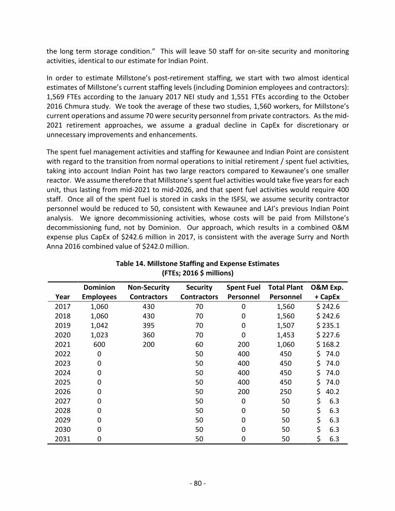
the long term storage condition.” This will leave 50 staff for on-site security and monitoring activities, identical to our estimate for Indian Point.
In order to estimate Millstone’s post-retirement staffing, we start with two almost identical estimates of Millstone’s current staffing levels (including Dominion employees and contractors): 1,569 FTEs according to the January 2017 NEI study and 1,551 FTEs according to the October 2016 Chmura study. We took the average of these two studies, 1,560 workers, for Millstone’s current operations and assume 70 were security personnel from private contractors. As the mid-2021 retirement approaches, we assume a gradual decline in CapEx for discretionary or unnecessary improvements and enhancements.
The spent fuel management activities and staffing for Kewaunee and Indian Point are consistent with regard to the transition from normal operations to initial retirement / spent fuel activities, taking into account Indian Point has two large reactors compared to Kewaunee’s one smaller reactor. We assume therefore that Millstone’s spent fuel activities would take five years for each unit, thus lasting from mid-2021 to mid-2026, and that spent fuel activities would require 400 staff. Once all of the spent fuel is stored in casks in the ISFSI, we assume security contractor personnel would be reduced to 50, consistent with Kewaunee and LAI’s previous Indian Point analysis. We ignore decommissioning activities, whose costs will be paid from Millstone’s decommissioning fund, not by Dominion. Our approach, which results in a combined O&M expense plus CapEx of $242.6 million in 2017, is consistent with the average Surry and North Anna 2016 combined value of $242.0 million.
Table 14. Millstone Staffing and Expense Estimates (FTEs; 2016 $ millions)
Year Dominion Employees
Non-Security Contractors
Security Contractors
Spent Fuel Personnel
Total Plant Personnel
O&M Exp. + CapEx
2017 1,060 430 70 0 1,560 $ 242.6 2018 1,060 430 70 0 1,560 $ 242.6 2019 1,042 395 70 0 1,507 $ 235.1 2020 1,023 360 70 0 1,453 $ 227.6 2021 600 200 60 200 1,060 $ 168.2 2022 0 50 400 450 $ 74.0 2023 0 50 400 450 $ 74.0 2024 0 50 400 450 $ 74.0 2025 0 50 400 450 $ 74.0 2026 0 50 200 250 $ 40.2 2027 0 50 0 50 $ 6.3 2028 0 50 0 50 $ 6.3 2029 0 50 0 50 $ 6.3 2030 0 50 0 50 $ 6.3 2031 0 50 0 50 $ 6.3
- 80 -

In order to estimate the cost of Millstone’s post-retirement personnel, we again relied on the NEI and Chmura studies.95 According to the January 2017 NEI study, Economic Impacts of the Millstone Power Station, “Millstone employs 1,569 full-time workers… The annual payroll and benefits are approximately $180 million. Most jobs at nuclear power plants require technical training and are typically among the highest-paying jobs in the area.” NEI divided the 1,569 workers into “…1,060 people in permanent jobs and 509 contractors…” with a payroll plus benefits of “approximately $180 million, and millions more for contract labor.” This is equivalent to approximately $169,811 per permanent Dominion worker, which appears high but may be explained by Millstone’s high proportion of workers with specialized skills and training.96
The Chmura study estimated that the Dominion employees had an average payroll (salaries, overtime, and benefits) of $168,365 excluding contractors, almost identical to NEI’s value.97 As a result, Chmura’s total payroll of $178.5 million for Dominion’s employees almost matches NEI’s total of approximately $180 million for Dominion employees. We assume that contractors (including security personnel) are paid less than Dominion employees to derive O&M expenses and CapEx assuming Millstone’s retirement in mid-2021.
2.6.1 Post-Retirement Non-Operating Expenses
It is unclear whether Millstone will continue to pay local property taxes in Waterford after retirement. Although the property taxes are based on real and personal property valuations, not on plant income, it seems unlikely that they will continue after retirement. We note that Dominion negotiated an agreement for its retired Kewaunee plant to gradually decrease its tax payments by 20% annually starting from the year after it shut down. Therefore we assume that Millstone’s property tax payments will also decline gradually, starting in 2021, by 20% annually while spent fuel activities are taking place.
Since Millstone will not be earning any income after mid-2021, we assumed income taxes would be zero after retirement.
As long as the nuclear power plant continues to be an NRC licensee, all financial protection requirements set forth in the NRC Regulations under 10 CFR Part 140 are applicable. The NRC license is terminated only after all decommissioning and decontamination conditions are met, which can take decades. Although Millstone will no longer operate, it will store its spent fuel onsite just like many other retired US nuclear power plants. For example, Yankee Atomic, Connecticut Yankee, and Maine Yankee that have retired continue to maintain active nuclear liability insurance policies with $100 million coverage. In addition, per 10 CFR 140.11, in 2017, the $375 million coverage for bodily injury, property and environmental damage is increased to
95 We note that these employment data do not affect our estimates for Millstone’s non-fuel O&M expenses or CapEx under continuing operations. 96 While the NEI study that claimed “…nuclear energy jobs pay 36 percent more than average salaries in a plant’s local area…”, we do not know if this percentage is applicable to Connecticut, a state with relatively high salaries. 97 The fact that NEI and Chmura have the same payroll values for Dominion employees may be explained by Dominion having provided the underlying data to both parties.
- 81 -

$450 million. Consistent with the NRC policy we will include the insurance premiums to be paid by Dominion for Millstone in the post-retirement period.
We assume that Dominion will incur very little G&A expenses after retirement and virtually no G&A expenses once all of the spent fuel is stored in the ISFSI.
- 82 -

3 MILLSTONE CASH FLOW ANALYSIS
Dominion is likely to consider many complex and interrelated issues in a decision to continue operation of or close down the Millstone station. A key driver would be expected net cash flows from the facility as a going concern. LAI has developed a cash flow model based on the cost categories and revenue types discussed in the preceding sections of this report to determine the magnitude and robustness of after-tax cash flows for Millstone. We have overlooked the bridge period, 2018 through mid-year 2021, focusing on the period 2021 through 2035.98 We find that net cash flows are consistently positive over the period under a wide range of energy market conditions and stress tests on key cost drivers.
3.1 MODEL STRUCTURE
The LAI cash flow model for Millstone calculates calendar year net cash flows from estimates of energy revenues, capacity revenues, fuel costs, operation and maintenance (O&M) expenses. Other line item expenses have also been calculated such as property taxes, sales and use taxes, insurance, allocated general and administrative (G&A) costs, on-going capital expenditures, and resulting federal and state income taxes.
The term for analysis is bound by the earliest reasonable retirement date. Because the ISO-NE reconfiguration auction is illiquid, LAI has made the simplifying assumption that the earliest feasible retirement date is the end of Millstone’s current CSO, i.e., May 31, 2021. The expiration date of the operating license for Millstone Unit 2 is 2035. While Unit 3 has an additional ten years of operating license term, as previously noted Dominion has stated that it would not consider operation with only a single unit at the site. Given the 3-year lead time to secure a CSO and the likely budgeting cycle for capital expenditures, LAI’s financial model “looks back” for 3 calendar years to include capital expenditures that would have to be committed to continue operation. Essentially, the CapEx budgeted for 2018 through 2034 is included as a negative cash flow, while operating cash flows begin in June 2021 and continue through May 2035.
All cash flows are calculated in nominal dollars and discounted to the end of May 2021. The discount rate is 7.00%. This rate is consistent with a 50% debt, 50% equity capital structure and a target equity return of about 10.5%. A general inflation rate of 2.00% is assumed in the model for adjusting costs originally estimated in 2017 dollars to nominal dollars.
In the financial model, we have ignored the book and tax values of the facility as of 2017. Capital expenditures beginning in 2018 are depreciated for tax purposes over a 20-year life by vintage
98 At the end of the study period when the retirement of both Millstone units is contemplated, Dominion would be positioned to write-off the remaining net book value of the units, thereby realizing a potentially large tax benefit at the parent level if, for whatever reason, a substantial portion of Dominion’s investment has not been depreciated. If Dominion were to accelerate the retirement decision it would also accelerate the realization of the tax benefit attributable to the undepreciated book value of the Millstone units. Whether or not the timing of such tax benefits has an impact on the retirement decision is unknown. Whether or not Dominion might at a later date decide to operate Millstone Unit 3 to 2045 is also unknown.
- 83 -

using 150% declining balance rates approximating MACRS rules. Upon retirement in 2035, any remaining undepreciated balance is captured and used as a tax loss in that year.
The model does not consider the level of on-going costs at Millstone that would be incurred by Dominion for several years after shutdown. We have assumed that these costs would be comparable in magnitude (in constant dollars) whether incurred after 2021 or after 2035. The difference in present value for incurring these costs starting in 2035, versus starting them in 2021 is separately estimated at $83.5 million on an after-tax basis.99
3.2 REFERENCE CASE
The energy and capacity market modeling assumptions for the Reference Case are defined in Section 1. These assumptions represent LAI’s expected or most likely outcome for market conditions. Hence, they support the determination of a most likely present value of cash flows associated with continued operation of Millstone over the relevant planning horizon.
The relative magnitudes of annual cash flow components are shown in Figure 55. The negative net cash flows in 2018, 2019, and 2020 represent the capital outlays for equipment upgrades and replacement that would likely be necessary to meet NRC regulations and to continue operation from 2021 through 2035. As shown in Figure 57, these capital outlays, represented by blue bars below the x-axis, continue through 2034. They are comparatively small relative to revenues and ongoing operating expenses. Revenues from sale of energy and capacity are shown in bright red and green, respectively, above the x-axis for 2021-2035. The amounts for the end years reflect 5 months of operation in 2021 and 7 months in 2035. Below the x-axis, the lowest bars represent O&M, fuel expense, and other expense. The other expenses reflect property taxes, insurance, and sales and use tax. The light brown bars represent income taxes, which are negative cash flows in most years, but positive in 2035. The positive in 2035 reflects a tax loss for undepreciated capital expenditures at retirement.
99 It is conservative to ignore such costs for the purpose of determining whether continued operation is viable.
- 84 -

Figure 55. Reference Case Millstone Annual Cash Flows
After-tax net cash flow is positive for years 2021 through 2035. The net present value in mid-2021, including the capital outlay in 2018-2020, is positive at $2,373 million. Hence, the Millstone enterprise value stated in mid-2021 is about $2.4 billion based on Reference Case assumptions.
A breakout of the present value is shown in Table 15.
Table 15. May 2021 Net Present Value
(Millions) Revenue Energy Sales $ 6,785 Capacity Sales $ 1,791 Total Revenue $ 8,576 Operating Expense Fuel ($ 1,195) O&M ($ 1,887) Other ($ 486) Total Expenses ($ 3,568) EBITDA $ 5,009 Income Taxes ($ 1,805) Capital Expenditures ($ 831) Net After-Tax Cash Flow $ 2,373
($1,000,000)
($500,000)
$0
$500,000
$1,000,000
$1,500,000
2018 2020 2022 2024 2026 2028 2030 2032 2034
Annu
al C
ash
Flow
($ 0
00)
CapacityRevenue
EnergyRevenue
O&M
Fuel
OtherExpenses
Total IncomeTax
CapitalInvestment
Net After-TaxCash Flow
- 85 -

Total taxes are summarized for the year 2022 and on a present value basis for 2021-2035 in Table 16.
Table 16. Taxes for 2022 and 2021-2035
2022 (Millions)
PV 2021-2035 (Millions)
Federal Income Tax $149.3 $1,406.9 State (CT) Income Tax $ 42.2 $ 397.5 Sales and Use Taxes $ 7.6 $ 73.5 Property Taxes $ 32.8 $ 316.8 Total Taxes $231.9 $2,194.7
3.3 SENSITIVITIES
As discussed in section 1.1.2, four sensitivities were developed to test the effect of external market variables on the robustness of estimated Millstone cash flows. The High Gas Price Case assumes that natural gas prices are significantly higher than anticipated in the Reference Case. The Low Gas Price Case, conversely, assumes significantly lower natural gas prices over the study term. In the EV Penetration Case, load forecasts are adjusted to reflect significant penetration of EV technology. In the High RE Development Case, large amounts of solar and wind resources are added to the capacity mix relative to the Reference Case. For each of these cases, the energy market and capacity market simulations were rerun to determine the change in Millstone’s revenues.
Annual Millstone net cash flows are shown for the Reference Case and the five sensitivities in Figure 56. Cash flows for 2021-2035 are highest for the High Gas Price Case and lowest for the Low Gas Price Case, reflecting the linkage between delivered natural gas costs in New England and energy prices. Cash flows for the EV Penetration Case and the High RE Development Case are close to those of the Reference Case. The EV Penetration Case cash flows reflect the slightly higher average electric loads, which raise energy prices, particularly in off-peak hours. The additional infra-marginal resources in the High RE Development Case tend to reduce energy prices in most hours, resulting in slightly lower revenues than those of the Reference Case.
- 86 -

Figure 56. Millstone Annual Net Cash Flow – Sensitivities
The sensitivities have a primary effect on Millstone’s energy revenues. There is a second-order effect, namely, income taxes. Differences in capacity revenue are small. As shown in Figure 57, the present value of net cash flows increases significantly to $4.2 billion for the High Gas Price Case and drops to $1.5 billion for the Low Gas Price Case. Hence, significant differences in delivered gas costs captured in the High v. Low Gas Price Cases have a material impact on enterprise value.
The present values of cash flows for the EV Penetration Case and the High RE Development Case are close to that of the Reference Case. The changes in factor inputs incorporated in the EV Penetration Case and the High RE Development Case do not have a significant impact on Millstone’s enterprise value.
The estimated present value from deferral of post-retirement costs of $83.5 million is not included in these figures, but would apply equally to all sensitivities.
($200,000)
($100,000)
$0
$100,000
$200,000
$300,000
$400,000
$500,000
$600,000
$700,000
$800,000
2018 2020 2022 2024 2026 2028 2030 2032 2034
Annu
al N
et C
ash
Flow
($ 0
00)
Reference CaseHigh Gas Price CaseLow Gas Price CaseEV Penetration CaseHigh RE Development Case
- 87 -

Figure 57. Present Values of Millstone Cash Flows – Sensitivities
3.4 STRESS TEST CASES
In addition to the sensitivities, which involved detailed modeling of external market variables, LAI also looked at certain “stress tests” involving changes to Millstone cost assumptions, while holding constant the external market results for either the Reference Case or the Low Gas Price Case. The focus of these tests was to determine if a substantial increase in assumed Millstone-specific costs would bring the annual and/or PV cash flows down to the point where there might be significant “missing money” from Millstone’s perspective.
We first assumed a 10% across-the-board increase in Millstone fuel, O&M, and Capital Expenditure costs under the Reference Case external variable assumptions. Relative to the Low Gas Price Case, we tested a 10% increase in CapEx, a 25% increase in CapEx, and a 10% across-the-board increase in fuel, O&M and CapEx. Present values of cash flow are compared for all of these stress test cases in Figure 58. Annual cash flows for the Low Gas Price Case test cases are shown in Figure 59. Note that the cash flows for years after 2020 are never negative, even with the extreme increases in Millstone cash costs. Millstone’s annual cash flows remain solidly in the black year-over-year, supporting an enterprise value of about $1.3 billion under worst-case assumptions. The present values also remain positive for all of the stress tests, suggesting that the Millstone cash flows are sufficiently robust to withstand a long term flattening out of delivered gas costs to New England coupled with a high, across-the-board increase in Millstone’s operating expenses, including CapEx.
$2,373
$4,235
$1,523 $2,513 $2,303
($10,000)
($5,000)
$0
$5,000
$10,000
$15,000
ReferenceCase
High Gas PriceCase
Low Gas PriceCase
EV PenetrationCase
High REDevelopment
Case
Pres
ent V
alue
of
Cash
Flo
w ($
MM
)CapacityRevenue
EnergyRevenue
O&M
Fuel
OtherExpenses
IncomeTaxes
CapitalInvestment
Net After-TaxCash Flow
- 88 -

Figure 58. Present Value of Millstone Cash Flows – Stress Test Cases
Figure 59. Annual Cash Flows – Low Gas Stress Test Cases
$2,3
73,3
67
$2,1
32,1
32
$1,5
22,8
97
$1,4
63,9
48
$1,3
75,5
23
$1,2
81,6
63
$0
$500,000
$1,000,000
$1,500,000
$2,000,000
$2,500,000
ReferenceCase, Base
Costs
ReferenceCase, 10%Increase in
CapEx,O&M,and Fuel
Low Gas PriceCase, Base
Costs
Low Gas PriceCase, 10%increase inCapEx only
Low Gas PriceCase, 25%increase inCapEx only
Low Gas PriceCase, 10%increase in
CapEx, O&M,and Fuel
Pres
ent V
alue
of N
et C
ash
Flow
($ 0
00)
Present value cash flows include CapEx outlays from 2018 forward and operating cash flows from June 1, 2021 through May 31, 2035. All cash flows are discounted to May 31, 2021 at 7.00% per year.
$0
$50,000
$100,000
$150,000
$200,000
$250,000
$300,000
$350,000
2022 2024 2026 2028 2030 2032 2034
Annu
al N
et C
ash
Flow
($ 0
00)
Low Gas Price Case, Base Costs
Low Gas Price Case, 10% increase in CapEx only
Low Gas Price Case, 25% increase in CapEx only
Low Gas Price Case, 10% increase in CapEx, O&M, and Fuel
Partial years of operation in 2021 and 2035 are not shown. CapEx for 2018-2021 is excluded in this chart, but is critical to continued operation after May, 2021.
- 89 -

Although unlikely, the across-the-board increase in Millstone’s operating expenses, in particular, nuclear fuel costs, each year from 2021 through 2035, produces a another meaningful benchmark regarding Millstone’s downside exposure under intentionally harsh market and operating cost assumptions. The recent decline in nuclear fuel costs is shown in Figure 60. According to data from the NEI, the cost of nuclear fuel for the average plant in the U.S. declined in real terms by 13.8% from 2013 through 2016.100 Uranium prices in terms of $/pound of U3O8 have been generally declining since reaching a peak of $136 for spot prices and $95 for long-term prices in June 2007. For these reasons and others, the 10% increase in nuclear fuel costs through 2035 appears far-fetched, but nevertheless relevant for purposes of assessing the resiliency of Millstone’s cash flows under harsh market and operating assumptions.
Figure 60. Uranium (U3O8) Prices (2013 - 2017)
100 The cost of uranium accounted for approximately 40% of the total cost of nuclear fuel in 2016.
- 90 -

4 MILLSTONE REPLACEMENT COST ANALYSIS
The early retirement of Millstone would likely result in higher costs of electricity for Connecticut ratepayers as well as higher emissions of carbon dioxide from other generators in both Connecticut and across New England. Quantifying that cost requires assumptions regarding how the energy markets would react to the loss of the largest baseload generation plant in New England, as well as how the State of Connecticut, acting through PURA, DEEP and the EDCs, might intervene to facilitate carbon reduction goals. LAI has developed a load cost model which allows for the comparison of futures with Millstone in service through 2035 or with Millstone retired in 2021 and three scenarios regarding State policy. In the 0% Replacement Case, it is assumed that the capacity and energy markets are allowed to work toward meeting any deficiencies with merchant natural gas-fired generation. In the 25% Replacement Case, the EDCs are mandated to procure a portfolio of renewable energy and demand side resources equivalent to one-quarter of the energy production lost from Millstone. In the 100% Replacement Case, the EDCs are mandated to procure a portfolio of hydro power (with transmission), renewable energy, and demand side resources equivalent to the full lost production from Millstone.
Ratepayer costs include the wholesale market value of the Connecticut EDC energy load, the FCM cost that would be assigned to that load, and the net costs incurred by the EDCs to procure mandated resources (including transmission services). LAI finds that the present value (in 2017) of the ratepayer costs associated with a mid-2021 retirement of Millstone Units 2 and 3, relative to their retirement in mid-2035, would be about $700 million. The ratepayer costs to implement the 25% Replacement Case would increase to $1.8 billion (excluding net participant costs for energy efficiency and passive demand response (EE/PDR) resources). Ratepayer costs for the 100% Replacement Case would be about $5.5 billion on the same basis.
The 25% Replacement Case would avoid roughly a quarter of the incremental CO2 emissions associated with the loss of Millstone energy output over the study period, while the 100% Replacement Case would avoid virtually all of those incremental CO2 emissions.
4.1 REPLACEMENT RESOURCE ASSUMPTIONS
LAI identified portfolios of clean energy resources that could be used to replace all or a portion of the 16 TWh/yr of Millstone energy production. Per guidance from the Technical Team, two replacement portfolios were analyzed. The first portfolio replaces 25% of Millstone’s energy production with non-emitting energy resources. One-half is derived from utility scale solar PV in Connecticut. The other half is from EE/PDR, as shown in Table 17.
Table 17. Non-Emitting Energy Resources in 25% Replacement Case
Technology Nameplate Additions (MW) Connecticut Utility-Scale Solar 1,206 EE/PDR 339
- 91 -

The second portfolio, listed in Table 18 replaces 100% of Millstone’s output with a diverse portfolio of non-emitting resources, approximately maintaining the region’s total carbon footprint.101
Table 18. Non-Emitting Energy Resources in 100% Replacement Case
Technology Nameplate Additions (MW) Incremental Clean Energy via HVDC Imports 1,000 Connecticut Utility-Scale Solar 2,412 EE/PDR 677 Off-Shore Wind 372
The replacement scenarios analyze costs and benefits of the portfolios from the ratepayer perspective. To estimate costs to ratepayers, we assume that these clean energy resources will be financed and developed only if supported by a long term (20 year) PPA with the EDCs. The EDCs would recover all PPA costs from distribution load as a non-bypassable charge. Benefits are derived as the mark-to-market value of the energy from the project, and RECs, if applicable.
4.1.1 CT Utility-Scale Solar
PPA costs for solar projects are based on the average of all of the selected projects from both the Clean Energy RFP and the small-scale (2-20 MW) renewable procurement under P.A. 15-107 Section b. There are 12 such projects located in Connecticut, with a combined total of 221 MW, and all are for 20-year terms. The weighted average levelized price (2017$) for bundled energy plus RECs is $96.40/MWh.
4.1.2 EE/PDR
One EE/PDR project was selected in the 2-20 MW renewable procurement. The levelized unit price for this project is $59.27/MWh (2017$). The unit price covers a 15-year contract term. Per guidance from the Technical Team, this cost does not include a participant’s contribution. This price was used as a starting incremental EE/PDR price in our forecast. In the Reference Case, we assumed that the EE/PDR penetration would be consistent with the ISO-NE 2017 CELT Load Forecast assumptions. In the 100% Replacement Case, the EE/PDR capacity of 677 MW was divided into three equal blocks of 266 MW entering each year over a three year period starting in 2021. In the 25% Replacement Case, the blocks were one-half that size. We have made the simplifying assumption that the incremental costs of the EE/PDR programs will escalate with the increased levels of penetration.
There is no single methodology broadly accepted by the industry for correlating the EE/PDR penetration rate and the incremental cost. The approaches vary from assuming no such correlation, i.e., the flat incremental cost assumption, to the very steep curves where prices raise
101 A “High OSW” portfolio was also considered, but not authorized by the Technical Team.
- 92 -

exponentially.102,103 The results show that the cumulative present value of incremental replacement EE/PDR utility-only costs amount to about $1.3 billion for the 25% Replacement Case and about $2.6 billion for the 100% Replacement Case.
The EE/PDR resources are modeled in accordance with the “Utility Cost Test”, which accounts for direct costs incurred by the utility, offset by the market value of the energy load avoided. Results are also presented reflecting the “Total Resource Cost Test” approach, which includes participant costs and other participant benefits, such as other components of avoided electric supply costs.
4.1.3 Imported Hydropower
None of the projects for new transmission infrastructure proposed to import large-scale hydropower into the New England region were selected in the CERFP. LAI reviewed information associated with new HVDC transmission projects as well as comparatively recent HVDC projects in neighboring RTOs. The levelized price of about $15/kW-mo was selected as representative of an HVDC project along the path and length appropriate in the present context. We have made the simplifying assumption that a zero carbon emission supply from Quebec transmitted from an HVDC project would qualify for a CSO, thereby supplanting incremental gas-fired generation to meet the net ICR. We have assumed that the price paid for the energy delivered will match the value of that energy at the delivery point.
4.1.4 Off-Shore Wind
OSW costs in the northeast have fallen significantly since Cape Wind was proposed in the mid-2000s. The 30 MW Block Island Wind Farm has successfully demonstrated the OSW concept. Earlier this year the Maryland PSC awarded 20-year OSW Renewable Energy Credit (OREC) purchase commitments to two OSW projects.104 The projects were the 248 MW US Wind project with 913,845 ORECs per year (P50) and the 120 MW Skipjack project with 455,482 ORECs per year (P50). The projects submitted the following price schedules to the Maryland PSC with different starting dates.
102 In our analysis, we assumed a blend of the flat price curve where the cost does not depend on the level of penetration, and a moderate curve proposed by Dr. Richard Stevie 103http://www.integralanalytics.com/files/documents/Projecting%20Energy%20Efficiency%20Program%20Costs%202015.pdf 104 Maryland PSC final Order No. 88192 in Case No. 9431. Maryland ratepayers will make up the difference between these OREC prices and the value of the energy and capacity imbedded in the ORECs.
- 93 -

Table 19. Maryland OSW Price Schedules ($/MWh)
Year US Wind Skipjack 2021 166.70 2022 168.37 2023 170.05 171.30 2024 171.75 173.01 2025 173.47 174.74 2026 175.20 176.49 2027 176.96 178.26 2028 178.72 180.04 2029 180.51 181.84 2030 182.32 183.66 2031 184.14 185.49 2032 185.98 187.35 2033 187.84 189.22 2034 189.72 191.11 2035 191.62 193.03 2036 193.53 194.96 2037 195.47 196.90 2038 197.42 198.87 2039 199.40 200.86 2040 201.39 202.87 2041 204.90 2042 206.95
The weighted levelized price, expressed in 2017 dollars, is $142.10/MWh. In our analysis, the price is escalated at 2% per year.105
4.2 MODEL STRUCTURE
The LAI ratepayer cost model for Millstone calculates calendar year costs for market energy and capacity purchases that would flow to ratepayers through Standard Service rates or competitive supplier rates,106 mandated resource costs, net of the market value of energy procured,107 that would flow to ratepayers through non-by-passable distribution charges. The model also accounts for the avoided energy benefits for EE/PDR projects sponsored under mandated incremental programs. In reviewing the results, this set of costs is labeled as “Net Utility Cost,” consistent with the Utility Cost Test for demand-side program analysis. We have also calculated a “Total
105 The resulting annual prices are reasonably consistent with a 2016 study prepared by the University of Delaware where the levelized cost of energy for a 400 MW tranche with a 2023 COD was reported to be $162.00 /MWh, including environmental attributes. 106 The market price effect (indirect benefit) for RECs was not considered. 107 The market value of RECs procured was not considered as an off-setting benefit.
- 94 -

Net Cost” that includes both the participant costs and the participant avoided capacity cost benefits for EE/PDR, consistent with the Total Resource Cost Test.
The term for analysis begins January 1, 2018, and runs through May 31, 2035, the end of Millstone’s Unit 2’s NRC license. LAI did not examine the operating costs and benefits associated with Millstone Unit 3’s operation after 2035.
All costs and benefits are calculated in nominal dollars and discounted to the end of 2017 at an annual rate of 7.00%. A general inflation rate of 2.00% is assumed for adjusting costs originally estimated in 2017 dollars to nominal dollars. Net costs and components are expressed in nominal dollars for each year, present value in 2017, or levelized constant 2017 dollars per unit.
Units can be MWh of Connecticut load, MWh of lost Millstone energy output, or short tons of CO2 emissions.
4.3 CASE DESCRIPTIONS
4.3.1 Reference Case
The energy and capacity market modeling assumptions for the Reference Case are defined in section 1. These assumptions represent LAI’s expected or most likely outcome for market conditions. They are used to determine a most likely present value of ratepayer costs associated with continued operation of Millstone through May 2035.
The energy cost-to-load for the Reference Case has a present value of $14.465 billion, equivalent to a levelized 2017 dollar unit cost of $40.65/MWh of Connecticut load. The capacity cost-to-load has a present value of $5.540 billion, equivalent to a levelized 2017 dollar unit cost of $15.57/MWh.
4.3.2 0% Replacement Case
In the 0% Replacement Case, Millstone is retired effective June 1, 2021. The loss of Millstone does not trigger the need for new capacity in Connecticut; however, the reserve margin in New England falls below the requisite ISO-NE Net ICR level. Natural gas-fired combined cycle plants are added to meet the Net ICR requirement. No incremental clean energy resources are added in Connecticut. The resulting costs are in the form of higher market energy prices and FCA capacity clearing prices. Such higher costs would be borne by Connecticut load through higher Standard Service or competitive supplier charges.
The energy cost-to-load increases to $14.757 billion, equivalent to a levelized 2017 dollar unit cost of $41.47/MWh of Connecticut load. The capacity cost-to-load increases to $5.967 billion, equivalent to a levelized 2017 dollar unit cost of $16.77/MWh. The total increase in ratepayer cost, relative to the Reference Case, is $719.2 million in 2017 present value. Annual nominal dollar costs are shown in Figure 61.
- 95 -

Figure 61. 0% Replacement Case Annual Cost
We have assumed that the natural gas-fired combined-cycle plants that are added to meet the Net ICR requirement would rely on New England’s existing pipeline infrastructure to meet their fuel needs.108 Figure 62 shows the incremental monthly average generator gas demand in the 0% Replacement Case relative to the Reference Case for Connecticut and Rhode Island, highlighting the 2022-23, 2027-28 and 2032-33 heating seasons. Figure 63 shows the monthly profile of incremental generator gas demand during each of the three selected winters.
108 Reoptimization of the New England gas grid to support new entry is the outside the scope of this inquiry.
($50)
$0
$50
$100
$150
$200
$250
2018 2020 2022 2024 2026 2028 2030 2032 2034
Diffe
rent
ial A
nnua
l Cos
t (Be
nefit
) -$
mill
ions
REC Cost-to-Load
CapacityCost-to-Load
Energy Cost-to-Load
Total NetCost
- 96 -

Figure 62. Incremental Generator Gas Demand in CT & RI, 0% Replacement Case
Figure 63. Incremental Generator Gas Demand in CT & RI for Selected Winters, 0% Replacement Case
-50
0
50
100
150
200
250
300
350
Jan-
18
Jan-
19
Jan-
20
Jan-
21
Jan-
22
Jan-
23
Jan-
24
Jan-
25
Jan-
26
Jan-
27
Jan-
28
Jan-
29
Jan-
30
Jan-
31
Jan-
32
Jan-
33
Jan-
34
Jan-
35
Incr
emen
tal D
eman
d Re
lativ
e to
Ref
eren
ce (
MD
th/d
)RhodeIslandConnSouthwestConnCentral
- 97 -

In order to place these incremental gas demands in the context of the existing New England pipeline infrastructure, Figure 64 adds the average monthly incremental generator gas demands for the selected winters to the actual daily flows through Algonquin’s Southeast compressor station from the 2016-17 heating season, and presents these demand levels relative to the 2016-17 daily throughput capacity of the compressor station. Figure 65 accounts for the capacity increase associated with Algonquin’s Atlantic Bridge Project, and adjusts the 2016-17 flow data to represent “Future Baseline Demand” by maintaining the 2016-17 daily utilization percentage relative to the increased capacity.109 These figures show that the incremental generator gas demand during all three future winters would place throughput consistently above the installed capacity of the pipeline, indicating the need for incremental capacity on Algonquin if the plants were to be dependent on this supply path.
Figure 64. Demand Relative to 2016-17 Algonquin Capacity, 0% Replacement Case
109 Average utilization of the Southeast compressor station during November 2017, after the in-service date of the Atlantic Bridge Project, was 92.6%. Average capacity utilization at the station during November 2016 was 92.5%.
0
500
1,000
1,500
2,000
2,500
November December January February March
CS C
apac
ity /
Gas
Flo
w (M
Dth
/d)
Southeast CS Flow (2016-17)
Southeast CS Capacity (2016-17)
2016-17 Flow + 2022-23 Incremental Demand
2016-17 Flow + 2027-28 Incremental Demand
2016-17 Flow + 2032-33 Incremenal Demand
- 98 -

Figure 65. Demand Relative to Future Algonquin Capacity, 0% Replacement Case
The generator additions could, however, could rely on a supply path other than via Algonquin. Expanding the analysis to encompass west-to-east flows and capacity on Algonquin, Iroquois and Tennessee yields Figure 66, which shows the effect of adding the incremental demand relative to 2016-17 flows and capacity. Figure 67 shows the effect of the incremental demand relative to baseline flows capacity following the completion of the Connecticut Expansion and Atlantic Bridge projects. These results indicate fewer days with insufficient capacity, but assume the absence of upstream constraints on Tennessee and economic viability of Iroquois receipts at Waddington throughout the heating season.
0
500
1,000
1,500
2,000
2,500
November December January February March
CS C
apac
ity /
Gas
Flo
w (M
Dth
/d)
Southeast Capacity w/ Atlantic Bridge
Future Baseline Demand
Future Baseline Demand + 2022-23 Incremental Demand
Future Baseline Demand + 2027-28 Incremental Demand
Future Baseline Demand + 2032-33 Incremental Demand
- 99 -

Figure 66. Demand Relative to 2016-17 AGT/IGT/TGP Capacity, 0% Replacement Case
Figure 67. Demand Relative to Future AGT/IGT/TGP Capacity, 0% Replacement Case
0
500
1,000
1,500
2,000
2,500
3,000
3,500
4,000
4,500
November December January February March
CS C
apac
ity /
Gas
Flo
w (M
Dth
/d)
Total AGT/IGT/TGP Flow (2016-17)Total AGT/IGT/TGP Capacity (2016-17)2016-17 Flow + 2022-23 Incremental Demand2016-17 Flow + 2027-28 Incremental Demand2016-17 Flow + 2032-33 Incremental Demand
0
500
1,000
1,500
2,000
2,500
3,000
3,500
4,000
4,500
November December January February March
CS C
apac
ity /
Gas
Flo
w (M
Dth
/d)
Total Capacity w/ Atlantic Bridge & Connecticut ExpansionFuture Baseline DemandFuture Baseline Demand + 2022-23 Incremental DemandFuture Baseline Demand + 2027-28 Incremental DemandFuture Baseline Demand + 2032-33 Incremental Demand
- 100 -

4.3.3 25% Replacement Case
In the 25% Replacement Case or Load Share Replacement, utility-scale solar and EE/PDR resources are procured by the Connecticut EDCs to displace some of the merchant gas-fired additions included in the 0% Replacement Case. Annual clean energy amounts are compared to the Reference Case in Figure 68. Note that the solar and EE/PDR resources are phased in years 2020 through 2023, resulting in a net increase in 2020, more than 25% of the Reference Case amount in 2021, and slightly less than 25% in 2022.
Figure 68. 25% Replacement Case Clean Energy by Year
Direct costs of the solar resources consist of the payments by the EDCs to developers under PPAs for energy and RECs. Direct costs of EE/PDR resources consist of the payments by the EDCs to induce providers and participants to install measures, but under the “Utility Cost Test”, do not include participant costs. The direct benefit from solar resources is the market value of the energy procured, which is resold by the EDCs in the wholesale spot market. The direct benefit from the EE/PDR resources is defined, under the “Utility Cost Test”, as the wholesale market value of the avoided energy load. In determining Total Net Cost for the “Total Resource Cost Test”, LAI has included both the participant costs and the participant avoided capacity cost benefit. Indirect effects relative to the Reference Case include the change in Energy Cost-to-Load and the change in Capacity Cost-to-Load. Annual net costs, relative to the Reference Case, are shown in Figure 69.
0
2
4
6
8
10
12
14
16
18
2018 2020 2022 2024 2026 2028 2030 2032 2034
Annu
al Z
ero
Carb
on E
nerg
y (M
Wh)
M
illio
ns
EE/PDR
Solar
Millstone
Millstone(ReferenceCase)
- 101 -

Figure 69. 25% Replacement Case Annual Cost
Similarly to the 0% Replacement Case, no assumptions have been made regarding pipeline capacity expansions that may be required to meet the fuel needs of the new plants in the 25% Replacement Case. Figure 70 shows the incremental monthly average generator gas demand in the 25% Replacement Case relative to the Reference Case for Connecticut and Rhode Island, highlighting the 2022-23, 2027-28 and 2032-33 heating seasons. The relative incremental generator gas demands for these winters are shown in Figure 71.
($100)
($50)
$0
$50
$100
$150
$200
$250
$300
$350
$400
$450
2018 2020 2022 2024 2026 2028 2030 2032 2034
Diffe
rent
ial A
nnua
l Cos
t (Be
nefit
) -$
mill
ion
EE/PDR ParticipantBenefit
EE/PDR ParticipantCost
EE/PDR Utility Costless Energy Benefit
Solar Net Energy &REC Cost
Capacity Cost-to-Load
Energy Cost-to-Load
Total Net Cost
Net Utility Cost
- 102 -

Figure 70. Incremental Generator Gas Demand in CT & RI, 25% Replacement Case
Figure 71. Incremental Generator Gas Demand in CT & RI for Selected Winters, 25% Replacement Case
-50
0
50
100
150
200
250
Jan-
18
Jan-
19
Jan-
20
Jan-
21
Jan-
22
Jan-
23
Jan-
24
Jan-
25
Jan-
26
Jan-
27
Jan-
28
Jan-
29
Jan-
30
Jan-
31
Jan-
32
Jan-
33
Jan-
34
Jan-
35
Incr
emen
tal D
eman
d Re
lativ
e to
Ref
eren
ce (
MD
th/d
)RhodeIsland
ConnSouthwest
ConnCentral
- 103 -

Figure 72 shows the level of throughput at Algonquin’s Southeast compressor station if the incremental generator gas demands for selected future years had been in effect during the 2016-17 heating season. Figure 73 shows the same analysis with the actual flows and capacity updated to reflect the addition of the Atlantic Bridge Project. These figures show that the incremental generator gas demand during all three future winters would place throughput consistently above the installed capacity of the pipeline, albeit to a lesser degree than in the 0% Replacement Case.
Figure 72. Demand Relative to 2016-17 Algonquin Capacity, 25% Replacement Case
0
500
1,000
1,500
2,000
2,500
November December January February March
CS C
apac
ity /
Gas
Flo
w (M
Dth
/d)
Southeast CS Flow (2016-17)
Southeast CS Capacity (2016-17)
2016-17 Flow + 2022-23 Incremental Demand
2016-17 Flow + 2027-28 Incremental Demand
2016-17 Flow + 2032-33 Incremenal Demand
- 104 -

Figure 73. Demand Relative to Future Algonquin Capacity, 25% Replacement Case
Figure 74 and Figure 75 show the same analysis relative to the total west-to-east flows and capacity on Algonquin, Iroquois and Tennessee.
0
500
1,000
1,500
2,000
2,500
November December January February March
CS C
apac
ity /
Gas
Flo
w (M
Dth
/d)
Southeast Capacity w/ Atlantic Bridge
Future Baseline Demand
Future Baseline Demand + 2022-23 Incremental Demand
Future Baseline Demand + 2027-28 Incremental Demand
Future Baseline Demand + 2032-33 Incremental Demand
- 105 -

Figure 74. Demand Relative to 2016-17 AGT/IGT/TGP Capacity, 25% Replacement Case
Figure 75. Demand Relative to Future AGT/IGT/TGP Capacity, 25% Replacement Case
0
500
1,000
1,500
2,000
2,500
3,000
3,500
4,000
4,500
November December January February March
CS C
apac
ity /
Gas
Flo
w (M
Dth
/d)
Total AGT/IGT/TGP Flow (2016-17)Total AGT/IGT/TGP Capacity (2016-17)2016-17 Flow + 2022-23 Incremental Demand2016-17 Flow + 2027-28 Incremental Demand2016-17 Flow + 2032-33 Incremenal Demand
0
500
1,000
1,500
2,000
2,500
3,000
3,500
4,000
4,500
November December January February March
CS C
apac
ity /
Gas
Flo
w (M
Dth
/d)
Total Capacity w/ Atlantic Bridge & Connecticut Expansion
Future Baseline Demand
Future Baseline Demand + 2022-23 Incremental Demand
Future Baseline Demand + 2027-28 Incremental Demand
Future Baseline Demand + 2032-33 Incremental Demand
- 106 -

4.3.4 100% Replacement Case
In the 100% Replacement Case, additional clean energy resources are assumed to be procured by the EDCs to replace fully Millstone’s energy production. Hydro resources in Canada are paired with incremental HVDC transmission capacity, and OSW resources are added, along with solar and EE/PDR resources above the levels from the 25% Replacement Case. Annual clean energy totals are shown in Figure 76. As with the 25% Replacement Case, resources are phased in over several years, but approximately match the lost Millstone output from 2024 forward.
Figure 76. 100% Replacement Case Clean Energy by Year
In addition to the direct costs and benefits of the solar and EE/PDR resources, this case includes direct costs for hydro energy and dedicated transmission services, as well as energy and RECs from OSW, all procured by the EDCs under long term contracts. Indirect effects relative to the Reference Case include the change in Energy Cost-to-Load and the change in Capacity Cost-to-Load. Annual net costs, relative to the Reference Case, are shown in Figure 77.
0
5
10
15
20
25
30
2018 2020 2022 2024 2026 2028 2030 2032 2034
Annu
al Z
ero
Carb
on E
nerg
y (M
Wh)
M
illio
ns
Hydro viaHVDC
OSW
EE/PDR
Solar
Millstone
Millstone(ReferenceCase)
- 107 -

Figure 77. 100% Replacement Case Annual Cost
4.4 COMPARISON OF RESULTS
4.4.1 Emissions
Annual CO2 emissions in Connecticut for each case are shown in Figure 78. The 100% Replacement Case effectively brings emissions back to the Reference Case levels after 2022, while the 25% Replacement Case is closer to the levels associated with the 0% Replacement Case. Similar results for all of New England are shown in Figure 79.
($200)
$0
$200
$400
$600
$800
$1,000
$1,200
$1,400
2018 2020 2022 2024 2026 2028 2030 2032 2034
Diffe
rent
ial A
nnua
l Cos
t (Be
nefit
) -$
mill
ion
EE/PDR ParticipantBenefitEE/PDR ParticipantCostEE/PDR Utility Costless Energy BenefitOSW Net Energyand REC CostSolar Net Energy &REC CostHydro Net EnergyCostTransmission Cost
REC Cost-to-Load
Capacity Cost-to-LoadEnergy Cost-to-Load
Total Net Cost
Net Utility Cost
- 108 -

Figure 78. Connecticut CO2 Emissions for All Cases
Figure 79. New England CO2 Emissions for All Cases
0
2
4
6
8
10
12
2018 2020 2022 2024 2026 2028 2030 2032 2034
Annu
al C
O2
Emis
sion
s (t
ons)
M
illio
ns
0% Replacement Case - CT Only
25% Replacement - CT Only
100% Replacement Case - CT Only
Reference Case - CT Only
0
5
10
15
20
25
30
35
2018 2020 2022 2024 2026 2028 2030 2032 2034
Annu
al C
O2
Emis
sion
s (t
ons)
M
illio
ns
0% Replacement Case - New England
25% Replacement Case - New England
100% Replacement Case - New England
Reference Case - New England
- 109 -

4.4.2 Annual and PV Net Cost
Annual Total Net Cost, relative to the Reference Case, is plotted for each case in Figure 80. Total Net Cost includes the participant costs and benefits for the EE/PDR resources in the 25% and 100% Replacement Cases. Figure 81 shows a breakout of various cost and benefit components of the differential 2017 present value of costs for the replacement cases. Both Net Utility Cost and Total Net Cost are shown.
Figure 80. Comparison of Annual Total Net Cost
($200)
$0
$200
$400
$600
$800
$1,000
$1,200
2018 2020 2022 2024 2026 2028 2030 2032 2034
Diffe
rent
ial A
nnua
l Cos
t (Be
nefit
) -$
mill
ions
100% Replacement Case25% Replacement Case0% Replacement Case
- 110 -

Figure 81. Present Value of Total Net Cost
4.4.3 Unit Cost Representations
It can be helpful to represent the cost differentials among the cases on a levelized unit cost basis. The “denominator” for unitizing the costs can be the MWh of Connecticut EDC load, the MWh of lost Millstone output, or the tons of avoided CO2 emissions.110
In Figure 82, the differential present value of total net cost between each replacement case and the Reference Case is divided by the present value-adjusted lost Millstone energy output to obtain a 2017 dollar cost per MWh of lost output. The cost for the 0% Replacement Case is
110 Levelized unit costs are calculated as the ratio of the present value of the relevant stream of annual costs to the “present value” of the relevant annual stream of unit quantities. Streams of annual costs expressed in nominal dollars are discounted at the nominal discount rate. To obtain constant dollar levelized unit costs, the unit quantity streams are discounted at the real discount rate. These present values of quantity streams are referred to as “PV-Adjusted” quantities in Table 20.
$719.2
$2,412.3
$6,785.3
$1,794.4
$5,470.9
($1,000)
$0
$1,000
$2,000
$3,000
$4,000
$5,000
$6,000
$7,000
$8,000
0% Replacement Case 25% ReplacementCase
100% ReplacementCase
Pres
ent V
alue
of D
iffer
entia
l Cos
t (Be
nefit
) -$
mill
ion
EE/PDR ParticipantBenefitEE/PDR ParticipantCostEE/PDR Utility Costless Energy BenefitOSW Net Energyand REC CostSolar Net Energy &REC CostHydro Net EnergyCostTransmission Cost
REC Cost-to-Load
Capacity Cost-to-LoadEnergy Cost-to-Load
Total Net Cost
Net Utility Cost
- 111 -

$5.02/MWh. The cost for the 25% Replacement Case is $16.85/MWh. The cost for the 100% Replacement Case is $47.40/MWh.
Figure 82. Costs per MWh of Lost Millstone Output
In Figure 83, the same differential present value total net costs are divided by the appropriate Connecticut EDC load (adjusted for EE/PDR) to obtain a 2017 dollar cost per MWh of load. The impact of the 0% Replacement Case is $2.02/MWh, while the cost for the 100% Replacement
$5.02
$16.85
$47.40
$0
$5
$10
$15
$20
$25
$30
$35
$40
$45
$50
0% Replacement Case 25% Replacement Case 100% Replacement Case
Leve
lized
201
7 $
Tota
l Net
Cos
t per
MW
h of
Los
t M
illst
one
Out
put (
$/M
Wh)
- 112 -

Case is $21.32/MWh. Hence, Connecticut EDC load would incur an additional $19.30/MWh to avoid the incremental CO2 emissions associated with the 0% Replacement Case.
Figure 83. Cost per MWh of Load
These costs of avoiding incremental CO2 emissions can also be expressed on a dollar per ton basis. The difference in total net cost between the 25% Replacement Case or the 100% Replacement Case and the 0% Replacement Case can be divided by the corresponding present value-adjusted emissions differentials to produce the results shown in Figure 84. The effective avoidance of the incremental emissions across New England associated with the loss of Millstone
$2.02
$7.16
$21.32
$0
$5
$10
$15
$20
$25
0% Replacement Case 25% Replacement Case 100% Replacement Case
Leve
lized
201
7 $
Tota
l Net
Cos
t per
MW
h of
Co
nnec
ticut
Load
($/M
Wh)
- 113 -

is about $109 per short ton. Note that for this calculation, we assume that the cost of avoided CO2 emissions across the entire ISO-NE region is borne solely by Connecticut EDC load.
Figure 84. Cost per Short Ton of Avoided CO2 Emissions
These calculations are summarized in Table 20 below.
Table 20. PV and Levelized Unit Cost Results
$2.02
$7.16
$21.32
$0
$5
$10
$15
$20
$25
Zero Replacement Case 25% Replacement Case 100% Replacement Case
Leve
lized
201
7 $
Tota
l Net
Cos
t per
MW
h of
Co
nnec
ticut
Load
($/M
Wh)
- 114 -

5 MILLSTONE ECONOMIC IMPACTS
5.1 APPROACH
Millstone’s prospective in-state spending on goods and services is likely to have positive secondary economic impacts in Connecticut, including higher business revenues, more jobs, and higher tax receipts relative to total in-state spending if Millstone were to retire. These impacts occur due to a “multiplier effect” that includes indirect effects in the supply chain and induced effects when households have more income to spend. Conversely, Millstone’s retirement could have negative economic impacts to the local economic to the extent laid-off workers are not rehired by other in-state companies. Also, the significant annual capital spend to maintain plant availability would materially decrease upon plant retirement, thereby subtracting the local component of CapEx. Finally, Millstone’s property tax payments to the Town of Waterford would wind down.
In order to estimate these secondary effects, LAI has used an economic input-output model that predicts changes in local area economic activity across all sectors of the local economic system. LAI utilizes IMPLAN, a leading model for analyzing multiplier effects resulting from a change in local direct expenditures.
The secondary economic impacts must be interpreted. In the Retirement Case, we recognize that most of the Millstone employees are highly trained and skilled, and would be likely to find gainful engineering employment in Connecticut relatively quickly in light of the strength of the defense contracting industry. These firms include General Dynamics Electric Boat in Groton, United Technologies / Aerospace Systems in Winsor Locks, Cheshire, and Danbury, United Technologies / Pratt & Whitney in Middletown and East Hartford, and Lockheed Martin / Sikorsky in Stratford. Certain of these firms are likely to require additional nuclear expertise to fulfill their contractual obligations to the Department of Defense. Rehiring would mitigate the secondary impacts derived in this section.
In structuring this analysis LAI has not attempted to quantify the economic benefits of in-state spending on zero emissions resources to replace Millstone generation.111 In the 25% Replacement Case, utility scale solar and incremental EE/DR would require substantial labor committed to the construction of these resources in Connecticut. The level of employment in solar and incremental EE/PDR during the operating phase would be low, however. In the 100% Replacement Case, additional solar and EE/PDR would be supplemented with HVDC and OSW in Massachusetts. These additional resources to replace all clean energy from Millstone would also generate direct, indirect and induced income effects in Connecticut and in New England at large, thereby lessening the adverse economic impact in Connecticut associated with the postulated loss of Millstone. Hence, the economic impacts presented in this section represent an incomplete
111 Quantification of economic benefits attributable to clean energy replacement technologies in Connecticut and New England was not part of the scope of work.
- 115 -

“gross effects” rather than a complete “net effects” analysis, which is proper in theory, but complex to perform.112
5.2 INPUTS / ASSUMPTIONS
LAI undertook a four-step process to estimate Millstone’s in-state spending under our Reference Case and Retirement Cases: first, estimate Millstone’s spending; second, divide spending into IMPLAN economic sectors, i.e., industry, households, government; third, allocate sector spending between in-state and out-of-state; and, fourth, allocate in-state spending between labor and non-labor, e.g., materials, services, and fees.
1. We relied on FERC Form 1 data from Dominion’s regulated nuclear stations (fuel and O&M), and on the Chmura’s report regarding CapEx.
2. We divided our estimates of Millstone’s spending into IMPLAN sectors based on an NEI study, Economic Benefits of Millstone Power Station, which utilized Millstone spending over the one-year period April 30, 2001 through March 31, 2002 to estimate Millstone’s in-state benefits.113 This NEI study divided Millstone’s spending of $357.1 million into ten IMPLAN sectors.114 $159.4 million (44.6%) of the total spending was spent in-state, mostly for operations.115
3. We divided spending between in-state and out-of-state sourcing of labor, materials and services. All fuel expenses were deemed out-of-state. For CapEx, we relied on the 2016 Chmura study that utilized Millstone data provided by Dominion. Chmura indicated that “58% of the capital expenditure is expected to be spent within the state.” This percentage is reasonable and consistent with recent (2014 and 2015) NEI economic studies of other
112 A complete net effects analysis is outside the scope of this inquiry. 113 Although the January 2017 NEI study, Economic Impacts of the Millstone Power Station and the October 2016 Chmura study, The Economic Impact of the Millstone Power Station in Connecticut both included socio-economic analyses, neither one provided a breakdown of Dominion’s spending. NEI used the REMI PI+ model and Chmura consultants used IMPLAN Pro to estimate Millstone’s socio-economic impacts. 114 LAI converted the old IMPLAN activity categories into new categories that cover 2013 – 2015 data years. 115 We confirmed the reasonableness of the NEI breakdowns into IMPLAN sectors. First, we examined Millstone’s fuel expenses, which rose from 14% of total spending in 2001/02 to 28% in 2016. This is consistent with the significant increase in uranium fuel costs, which was about flat until 2005 and then quadrupled by 2011, before easing in 2016. Next, we examined O&M expenses plus CapEx, which decreased slightly from 2001/02 to 2016 and fell from 77% to 60% of total plant costs. Lastly, we examined non-operating expenses, i.e., G&A, property taxes, sales & use, and insurance.
- 116 -

nuclear plants.116 Chmura did not provide an in-state versus out-of-state allocation for O&M expenses.117
Therefore, LAI relied on those recent NEI economic studies for the Duane Arnold, St. Lucie, and Turkey Point nuclear plants to allocate Millstone’s non-fuel O&M expenses between in-state and out-of-state. We found that compensation accounts for the single largest share of O&M expenses. Compensation is virtually entirely in-state. We also found that total non-fuel O&M expenses (labor compensation plus materials) plus CapEx were allocated 71% in-state and 29% out-of-state. Our 2017 estimate of Millstone’s in-state non-fuel O&M plus CapEx spending of $171.6 million is 71% of its total spending of $243 million.
Table 21. LAI Estimate of Millstone’s Current Annual In-State Expenditures (2017 $ millions)
Spending Category Total In-State In-State CapEx $ 65.1 58.0% $ 37.7 Compensation $116.4 99.6% $115.9 Other O&M Expenses $ 61.2 29.4% $ 18.0 Total $242.6 $171.6
4. Our last step was to allocate in-state spending between labor and non-labor. Based on the NEI and Chmura studies, as well as our experience, we assumed that compensation for plant operations and professional services, e.g., business, management, consulting, architectural and security services, was 100% labor. We assumed that maintenance and repair construction, machinery and equipment, and similar spending were 15% labor and 85% non-labor. The net result is that 86% of all in-state spending prior to retirement was allocated to labor and 14% was allocated to materials.
Table 22. Historical Allocation of Millstone Expenditures (April 2001 - March 2002)
IMPLAN Sector In-State Spending Labor Non-Labor
($ millions) % % % 43 Operations (Compensation) $ 96.4 60.5 100 0 62 Maintenance and Repair $ 23.7 14.9 15 85 465, etc. Professional Services118 $ 37.2 22.7 100 0
116 LAI reviewed an April 2015 NEI economic study of the St. Lucie and Turkey Point plants and a May 2014 NEI economic study of the Duane Arnold plant. 117 Chmura lumped together Millstone’s O&M expense and generation output to estimate direct in-state spending of $1,010.4 million, which renders this data of limited or no use for allocating O&M expenses between in-state and out-of-state. 118 Includes 465 Business Support Services, 454 Mgt Consulting Services, 464 Employment Services, 449 Architectural and Engineering Services, 467 Investigation and Security Services, etc.
- 117 -

445, etc. Machinery and Equipment119 $ 2.1 1.3 0 100 Total $159.4 100.0
For the Millstone Reference Case in which the plant operates through 2035, we applied the NEI percentage breakdowns for all of the IMPLAN sectors. For the Millstone Retirement Case, we assumed that virtually all of Millstone’s spending after retirement would be to cool, cask, and store spent fuel, plus a small amount for security contractors.
5.3 RESULTS – REFERENCE CASE
LAI estimated that Millstone will create in-state annual outputs of $350.7 million (2017 $) from 2018 through 2032, almost evenly divided between direct and indirect / induced outputs.120 Total in-state plant output will decline slightly in 2033 as CapEx tapers off as the plant prepares for retirement, and will decline even further in 2036 through 2040 as Millstone ceases to operate, thus retaining a smaller staff for spent fuel activities and security.
The annual in-state Reference Case IMPLAN output results are summarized in Table 23.
Table 23. LAI Estimates of Millstone Annual In-State Output – Reference Case (2017$ millions)
2018-32 2033 2034 2035 2036-40 Direct $173.8 $155.3 $150.4 $111.1 $ 48.3 Indirect $ 40.9 $ 35.3 $ 34.2 $ 25.3 $ 14.7 Induced $136.0 $121.1 $117.3 $86.7 $ 32.8 Total $350.7 $311.8 $301.8 $223.1 $ 95.7
LAI estimated that for each direct job there will be approximately 1.5 indirect / induced jobs in-state through the 2035 Reference Case retirement date. Millstone’s economic benefits for the Reference Case, in terms of manufacturing, services, and retail / wholesale trade, has a PV of $4.2 billion (2017 $). This number, $4.2 billion, represents the total present value benefit associated with Millstone’s continued operation under the business-as-usual condition. It does not represent Connecticut’s exposure to adverse financial impacts if Millstone were to retire in 2021.
5.4 RESULTS – RETIREMENT CASE
LAI estimated that Millstone will create total in-state annual outputs of $350.7 million (2017 $) in 2018, falling slightly in 2018 as CapEx tapers off prior to retirement. By mid-2021, Millstone’s compensation will be reduced significantly as the plant ceases operations. At that point, in-state plant output will decline to $98.8 million and stay at this level through 2025 while a small staff handles spent fuel activities. We assume those activities will be completed in 2026 and by 2027
119 Includes 445 Commercial and Industrial Machinery and Equipment, 162 Industrial Gas Manufacturing, and 260 Fabricated Pipe and Fittings. 120 Although “value-added” is usually relevant, LAI has presented the results as output/sales to facilitate comparison with other measurements performed by NEI and Chmura.
- 118 -

only site maintenance and security are required, reducing in-state output to $8.8 million through 2040. Our annual in-state Retirement Case IMPLAN output results are summarized in Table 24.
Table 24. LAI Estimates of Millstone Annual In-State Output – Retirement Case (2017$ millions)
2018 2019 2020 2021 2022-25 2026 2027-40 Direct $173.8 $167.2 $160.7 $117.9 $ 49.8 $ 26.9 $ 4.2 Indirect $ 40.9 $ 39.3 $ 37.8 $ 27.7 $ 15.1 $ 8.2 $0.9 Induced $136.0 $131.0 $126.0 $ 92.5 $ 33.8 $ 18.2 3.7 Total $350.7 $337.4 $324.4 $238.1 $ 98.8 $ 53.3 8.8
LAI estimated that for each direct job there will be approximately 1.5 indirect / induced jobs in-state through 2021 and fewer indirect / induced jobs thereafter. Millstone’s economic benefits for the Retirement Case, in terms of manufacturing, services, and retail / wholesale trade, has a PV of $1.5 billion million (2017 $).
5.5 OUTPUT COMPARISON OF REFERENCE AND RETIREMENT CASES
Over the 2018 – 2040 study period, a comparison between estimated total in-state annual outputs in the Reference and Retirement Cases reveals a total difference of $ 2.7 billion (PV 2017 $). This difference ignores the likelihood that laid-off employees will find other employment in Connecticut’s defense industry. It also ignores the economic benefits if Connecticut pursues a more aggressive replacement strategy such as those delineated in the 25% or 100% Replacement Cases. Under these simplifying assumptions, the year by year direct, indirect and induced differences in 2017$ are shown in Figure 85 below. With these limitations, the in-state industries that would be most affected by Millstone’s retirement would be maintenance services, professional support services, housing, and other retail / wholesale services.
- 119 -
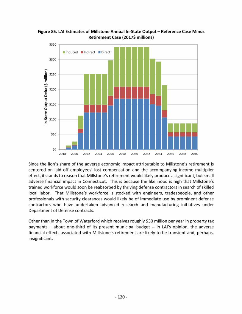
Figure 85. LAI Estimates of Millstone Annual In-State Output – Reference Case Minus Retirement Case (2017$ millions)
Since the lion’s share of the adverse economic impact attributable to Millstone’s retirement is centered on laid off employees’ lost compensation and the accompanying income multiplier effect, it stands to reason that Millstone’s retirement would likely produce a significant, but small adverse financial impact in Connecticut. This is because the likelihood is high that Millstone’s trained workforce would soon be reabsorbed by thriving defense contractors in search of skilled local labor. That Millstone’s workforce is stocked with engineers, tradespeople, and other professionals with security clearances would likely be of immediate use by prominent defense contractors who have undertaken advanced research and manufacturing initiatives under Department of Defense contracts.
Other than in the Town of Waterford which receives roughly $30 million per year in property tax payments – about one-third of its present municipal budget -- in LAI’s opinion, the adverse financial effects associated with Millstone’s retirement are likely to be transient and, perhaps, insignificant.
$0
$50
$100
$150
$200
$250
$300
$350
2018 2020 2022 2024 2026 2028 2030 2032 2034 2036 2038 2040
In-S
tate
Out
put D
elta
($ m
illio
n)Induced Indirect Direct
- 120 -

6 OUTLOOK ON NUCLEAR RETIREMENTS
Over the last few years, many nuclear power plants have been retired or have announced retirement. These include: Vermont Yankee and Pilgrim in ISO-NE: Gina, Fitzpatrick, Indian Point, and Nine Mile Point in NYISO; Kewaunee, Clinton, Byron, Quad Cities, and Palisades in MISO; Oyster Creek, Davis-Besse, and Three Mile Island in PJM; San Onofre and Diablo Canyon in CAISO; and a number of other plants, for example, Crystal River in Florida and Fort Calhoun in Nebraska. There may be others.
There are a number of primary reasons that explain nuclear plant retirements.
Regarding scale, small, single-unit plants around 600 MW or less suffer diseconomies of scale relative to two or three large (1,000-1,200 MW) units at a site. An owner’s inability to leverage the supply chain causes weakened financial performance. The age of the reactor and the high unit cost for small scale units may not support NRC license extension.
Regarding market dynamics, energy prices have decreased across the U.S. due to prolific shale gas production out of Marcellus and Utica basins, as well as other shale producing basins in the North Central states and Texas, thereby reducing net margin from energy sales. Renewable entry in various states, in particular, California, has heightened competitive pressures on the nuclear fleet. Also, nuclear plants rely on capacity revenue to ensure healthy financial performance. Capacity price mechanisms in many parts of the U.S. are evolving or are broken, reflecting a MW overhang in many parts of the U.S. where nuclear plants compete on a merchant basis. Those utilities that remain regulated under traditional cost of service regulation are impervious to weak price signals in regional capacity markets.
Regarding other reasons, a retirement decision may be sensible when there is a heavy prospective CapEx on the horizon to replace equipment or to comply with environmental requirements. Also, concerns about proximity to earthquake fault zones explain retirement decisions. More restrictive state policies that discourage nuclear plants close to population centers or environmentally sensitive areas also explain retirement decisions.
As discussed in Section 2.2.3, Millstone’s total nameplate and integral place in the Dominion portfolio supports a scale economy. This scale economy has helped sustain Millstone’s financial success. Independent economic analysis shows strong financial performance through 2035 even under intentionally harsh market and operating assumptions. LAI notes that Millstone does not have significant Pay-for-Performance risk and is, in fact, systematically benefited under ISO-NE’s FCA.
If, for the sake of argument, Millstone were required to invest in a new cooling water system, such capital-intensive investment would surely change the financial results presented in this inquiry. We are not aware of any other potential risk related expenditure that would cause Millstone’s CapEx to rise at a rate significantly higher than inflation.
- 121 -

- 122 -