resource allocation in multi-antenna communication...
TRANSCRIPT

Resource Allocation inMulti-Antenna CommunicationSystems with Limited Feedback
DAVID HAMMARWALL
Doctoral ThesisStockholm, Sweden October 2007


Resource Allocation in Multi-AntennaCommunication Systems with Limited Feedback
DAVID HAMMARWALL
Doctoral Thesis in TelecommunicationsStockholm, Sweden 2007

TRITA-EE 2007:051ISSN 1653-5146ISBN 978-91-7178-754-5
KTH, School of Electrical EngineeringSignal Processing Laboratory
SE-100 44 StockholmSWEDEN
Akademisk avhandling som med tillstånd av Kungl Tekniska högskolan framläggestill offentlig granskning för avläggande av teknologie doktorsexamen i telekommu-nikation måndagen den 1 oktober 2007 klockan 13:15 i hörsal F3, Lindstedtsvägen26, Stockholm.
© David Hammarwall, oktober 2007
Tryck: Universitetsservice US AB

iii
Abstract
The use of multiple transmit antennas is considered a key ingredient tosignificantly improve the spectral efficiency of wireless communication systemsbeyond that of currently employed systems. Transmit beamforming schemeshave been proposed to exploit the spatial characteristics of multi-antenna ra-dio channels; that is, multiple-input single-output (MISO) channels. In mul-tiuser communication systems, the downlink throughput can be significantlyincreased by simultaneously transmitting to several users in the same time-frequency slot, by means of spatial-division multi-access (SDMA). SeveralSDMA beamforming algorithms are available for joint optimal beamformingand power control for the downlink. Such optimal beamforming minimizes thetotal transmission power, while ensuring an individual target quality of ser-vice (QoS) for each user; alternatively the weakest QoS is maximized, subjectto a transmit power constraint.
In this thesis, both of these formulations are considered and some ofthe available algorithms are generalized to enable quadratic shaping con-straints on the beamformers. By imposing additional constraints, the QoSmeasure can be extended to take factors other than the customary signal tointerference-plus-noise ratio (SINR) into account. Alternatively, other limi-tations such as interference requirements or physical constraints may be in-corporated in the optimization. The proposed beamforming algorithms arealso based on a more general SINR expression than previously analyzed inthis context. The generalized SINR expression allows for more accurate mod-eling; for example, non-zero self interference can be modeled in code-divisionmulti-access (CDMA) systems.
A major limiting factor for downlink resource allocation is the amountof channel-state information (CSI) available at the base station. In mostcases, CSI can be estimated only at the receivers, and then fed back to thebase station. This procedure typically constrains the amount of CSI thatcan be conveyed. In this thesis, a minimum mean squared-error (MMSE)SINR estimation framework is proposed, which combines partial CSI withchannel-distribution information (CDI); the CDI varies slowly and is assumedto be known at the transmitter. User selection (scheduling) and beamformingtechniques, suitable for the MMSE SINR estimates, are also proposed.
Special attention is given to the feedback of a scalar channel-gain infor-mation (CGI) parameter. The CSI provided by CGI feedback is studied indepth for correlated Rayleigh and Ricean fading channels. It is shown, usingasymptotic analysis, that large realizations of the CGI parameter convey ad-ditional spatial CSI at the transmitter; the proposed scheme is thus ideal formultiuser diversity transmission schemes, where resources are allocated onlyto users experiencing favorable channel conditions. It is shown by numericalsimulations that, in wide-area scenarios, feeding back a single scalar CGI pa-rameter per user, provides sufficient information for the proposed downlinkresource-allocation algorithms to perform efficient SDMA beamforming anduser selection.

iv
Acknowledgments
It is truly a rewarding experience to be a PhD student in the creativesetting of the signal processing group at KTH. The group is a perfect matchof social people and academic excellence. First, I would like to extend mygratitude to my supervisor Professor Björn Ottersten, for taking me on as aPhD student. I am amazed by your generosity of your time; regardless of howbusy you actually are, you have always kept your office door invitingly open.Special thanks also to my assistant supervisor, Professor Mats Bengtsson. Ifnot for your good advice, on topics ranging from big research problems totiny LATEX issues, much effort would have been of no avail.
I would like to thank all my friends and colleagues in the communicationtheory and signal processing groups; it has been fantastic to work with youall. Joakim Jaldén deserves special mentioning. Our numerous discussions onintricate mathematical problems, throughout the years, have always been fun.Who knows? If not for our healthy competition during our undergraduatestudies, I might not have ended up writing this thesis.
I also want to extend special thanks to all of you who have proof read var-ious parts of the thesis: Emil Björnson, Svante Bergman, Joakim Jaldén,Niklas Jaldén, Klas Johansson, Simon Järmyr, Bengt Samuelsson, KarlWerner, Peter von Wrycza, and Xi Zhang. I have enjoyed my theoreticaldiscussions with Eduard Jorswieck and my hardware implementation endeav-ors cheered on by Per Zetterberg. I thank the computer support group, An-dreas Stenhall and Nina Unkuri, for the smoothly running system, and KarinDemin, Annika Augustsson and Anna Thöresson-Bergh, for helping out withall administrative issues.
I wish to thank Professor David Gesbert for taking the time to act as op-ponent for this thesis, and also Professor Mikael Johansson, Professor MarkkuJuntti, and Professor Mikael Sternad for participating in the committee.
To conclude, I want to thank my parents and brothers for always beingthere, for worrying about me, and for always whishing me the very best.Finally, I want to express my greatest love and gratitude to my wife Anna.Your love, support, and patience during this time, have truly been remarkable.
David HammarwallStockholm, September 2007
Contents
Contents v
1 Introduction 11.1 Digital Communication over Wireless Channels . . . . . . . . . . . . 41.2 Channel Quality Measures and Performance Limits . . . . . . . . . . 71.3 Scheduling in Multiuser Systems . . . . . . . . . . . . . . . . . . . . 81.4 Digital Communication using Multiple Antennas . . . . . . . . . . . 91.5 Multiuser Techniques for Wideband Channels . . . . . . . . . . . . . 121.6 Statistical Modeling of the Wireless Channel . . . . . . . . . . . . . 171.7 Statistical Channel Knowledge at the Transmitter . . . . . . . . . . 181.8 Feedback of Channel-State Information . . . . . . . . . . . . . . . . 191.9 SINR Estimation . . . . . . . . . . . . . . . . . . . . . . . . . . . . . 201.10 Outline and Contributions . . . . . . . . . . . . . . . . . . . . . . . . 211.11 Contributions Outside the Scope of the Thesis . . . . . . . . . . . . 27
2 Optimal Beamforming with Side Constraints 292.1 Introduction to Optimal Beamforming . . . . . . . . . . . . . . . . . 292.2 Problem Formulation . . . . . . . . . . . . . . . . . . . . . . . . . . . 302.3 Beamforming Using Semidefinite Programming . . . . . . . . . . . . 372.4 Beamforming Using the Virtual-Uplink Domain . . . . . . . . . . . . 392.5 Optimized Weighted Sum-Rate Beamforming . . . . . . . . . . . . . 442.A Lemmas for Proof of Strong Duality for P . . . . . . . . . . . . . . . 462.B Proof of Strong Duality for G . . . . . . . . . . . . . . . . . . . . . . 482.C Proof of Theorem 2.8 . . . . . . . . . . . . . . . . . . . . . . . . . . . 49
3 Applications for Constrained Beamforming 533.1 Path Diversity in DS-CDMA . . . . . . . . . . . . . . . . . . . . . . 533.2 Interference Constraints . . . . . . . . . . . . . . . . . . . . . . . . . 57
4 User Selection with MMSE SINR Estimation 634.1 System Assumptions . . . . . . . . . . . . . . . . . . . . . . . . . . . 644.2 System Design with MMSE SINR Estimation . . . . . . . . . . . . . 65
v

vi Contents
5 Low-Complexity Beamforming 715.1 Generalized Zero Forcing . . . . . . . . . . . . . . . . . . . . . . . . . 715.2 Virtual-Uplink MVDR Beamforming . . . . . . . . . . . . . . . . . . 765.3 One-Shot Beamforming . . . . . . . . . . . . . . . . . . . . . . . . . 77
6 MMSE SINR Estimation with CGI Feedback 816.1 Channel Model . . . . . . . . . . . . . . . . . . . . . . . . . . . . . . 826.2 The Conditional Channel Distribution . . . . . . . . . . . . . . . . . 836.3 Zero-Mean Channels . . . . . . . . . . . . . . . . . . . . . . . . . . . 886.4 Asymptotic Analysis . . . . . . . . . . . . . . . . . . . . . . . . . . . 926.5 Channels with Non-Zero Mean . . . . . . . . . . . . . . . . . . . . . 956.A Lemmas for Proof of Theorem 6.4 . . . . . . . . . . . . . . . . . . . 986.B Generating Realizations of the Conditional Distribution . . . . . . . 1016.C Lemmas for the Derivations of Conditional PDFs . . . . . . . . . . . 1026.D Proof of Theorem 6.5 . . . . . . . . . . . . . . . . . . . . . . . . . . . 1046.E Proofs of Corollaries . . . . . . . . . . . . . . . . . . . . . . . . . . . 1056.F Proof of Theorem 6.10 . . . . . . . . . . . . . . . . . . . . . . . . . . 107
7 Performance Evaluation 1137.1 Comparison of GZF and MVDR Beamforming . . . . . . . . . . . . 1147.2 System Evaluation . . . . . . . . . . . . . . . . . . . . . . . . . . . . 1177.3 Finite Rate Feedback . . . . . . . . . . . . . . . . . . . . . . . . . . . 125
8 Generalization of the CGI Parameter 1298.1 Computing the Conditional Moments . . . . . . . . . . . . . . . . . . 1308.2 Performance Evaluation of Pilot Signaling on Selected Antennas . . 1338.3 Approximation for Reduced Complexity . . . . . . . . . . . . . . . . 1348.A Proof of Theorem 8.1 . . . . . . . . . . . . . . . . . . . . . . . . . . . 1378.B Proof of Corollary 8.2 . . . . . . . . . . . . . . . . . . . . . . . . . . 1388.C Proof of Corollary 8.3 . . . . . . . . . . . . . . . . . . . . . . . . . . 139
9 Thesis Conclusions 141
A Nomenclature 143A.1 Notation . . . . . . . . . . . . . . . . . . . . . . . . . . . . . . . . . . 143A.2 Thesis Specific Symbols and Functions . . . . . . . . . . . . . . . . . 146A.3 Abbreviations and Acronyms . . . . . . . . . . . . . . . . . . . . . . 148
B Matrix Relations 151
C DS-CDMA Model 153C.1 Descrambling and RAKE Combining . . . . . . . . . . . . . . . . . . 153C.2 Long-Term SINR in DS-CDMA systems . . . . . . . . . . . . . . . . 155
Bibliography 157

Chapter 1
Introduction
Digital communication has become an essential part of the lifestyle in most partsof the world. The desire to access information and media around the globe, in thecomfort of the home or the office, has lead to an exponential increase in the useof the Internet and other data services. The demand for such services has inspiredtelecom operators of large-scale wireless systems to seek new revenue by extendingtheir service selection from the traditional voice service to provide data services onan anywhere-anytime basis.
The introduction of data services is a major motivating factor for the transitionfrom second generation’s GSM and cdmaOne (IS-95) cellular systems to third gen-eration’s WCDMA (UMTS) and CDMA2000 systems. The first iteration of UMTSsystems1 feature a peak downlink throughput of 384 kbit/s, which enables Inter-net access, low resolution media streaming, and video telephony. These systemsare optimized for circuit-switched voice, but many of the envisioned wireless dataservices pose different constraints than those of real time user-to-user communi-cation; for instance, packet based one-way streaming is not as delay sensitive astwo-way voice conversations. Services based on such elastic traffic are often bet-ter suited for a packet-switched best-effort system, rather than a circuit-switchedsystem. The resource scheduler can use the flexibility of elastic traffic to schedulethe transmission of a packet to a time (and frequency) slot where the fluctuatingwireless link has favorable conditions. The so-obtained diversity is often referredto as multiuser diversity2 [KH95]: If there are many users, at least one is likely toexperience favorable conditions.
The frequency spectrum that is utilized by large-scale wireless systems is a scarceresource; simply increasing the bandwidth3 is therefore not a feasible approach to
1 We refer to release 99 of the UMTS standard.2 Multiuser diversity is an integral part of the scheduling in the high-speed downlink packet ac-
cess (HSDPA) [FPR+01] and high-speed packet access (HSPA) [DPSB07] evolutions of WCDMA.3 With battery powered user terminals, the transmission power must be minimal to maintain
a reasonable battery life time. This power constraint also limits the bandwidth that can by usedby a terminal at a given transmit power per bandwidth ratio.
1

2 CHAPTER 1. INTRODUCTION
Figure 1.1: Illustration of the considered system. We consider a single cell, wherethe base station (transmitter) has an array of antennas, and the users (receivers)have a single receive antenna each.
push the performance of cellular wireless systems to match, or even surpass, that ofstate-of-the-art wired ADSL and VDSL systems. To achieve such performance, thespectrum must instead be used more efficiently. A promising technique to achieveincreased spectral efficiency, is to use multiple antennas (i.e., antenna arrays) at thebase stations. Figure 1.1, illustrates the multi-antenna system that is considered inthis thesis.
With multiple antennas, the spatial dimensions of the wireless propagation chan-nel can be exploited; for instance, if a base station has sufficient information of themulti-antenna wireless propagation channels, it can establish non-interfering linksto several users, in the same time (and frequency) slot; the users are instead sep-arated in space. This multi-access scheme is referred to as spatial-division multi-access (SDMA) [God97a, God97b].
A commonly used technique to exploit the spatial channel dimensions, is trans-mit beamforming, which focuses the radiated power into a beam, aimed at theintended user. This is achieved by ensuring that the signals from the differentantennas add constructively in the intended direction. Similarly, the radiation pat-tern can be shaped so as to form nulls (i.e., signal cancellation) in the directions ofinterfered users.
Multiple antenna schemes are core components of forthcoming communicationsystems—such as, long-term evolution (LTE) [DPSB07], which is currently beingstandardized within 3GPP4; and the system considered within the European UnionWINNER5 projects. In these next generation (or evolved) systems, we also seea shift in multi-access technique: Code-division multi-access (CDMA)—used inWCDMA and CDMA2000—is abandoned in favor of orthogonal frequency-divisionmulti-access (OFDMA) [SSO+07].
Using multiple antennas at the base stations for SDMA is not without difficul-
4 Third generation partnership project (3GPP).5 Wireless initiative new radio (WINNER).

3
ties:
• the base stations must acquire sufficient knowledge of the wireless propagationchannels to separate the signals of the different users. Moreover to exploit themultiuser diversity, the base stations have to continuously track the variations(the fading) of the wireless channels.
• the base stations must be able to utilize the available information; that is,they must know how to use the multiple antennas to achieve the performancepotentials.
In this thesis we address both of these issues. We distinguish between the downlink,6which is the link from the base station to the user terminals, and the uplink,7 whichis the link from the user terminals to the base stations. The resource scheduling isperformed in the base stations, therefore the previously mentioned difficulties withSDMA have significantly different implications in the uplink and the downlink.
In general, implementing SDMA in the uplink is less difficult than in the down-link, because the base stations can typically measure the required uplink channelinformation from pilot signals that are continually transmitted by the user termi-nals. Moreover, the signal processing required to separate users in the uplink issignificantly easier than the downlink counterpart (see e.g., [SB04] or Chapter 2 ofthis thesis).
In this thesis we consider the more demanding downlink. The considered system,which is illustrated in Figure 1.1, can be characterized as follows:
• The base station (transmitter) is equipped with multiple antennas.
• The users (receivers) each have a single antenna.
• The deployment is in a wide-area, or a metropolitan-area, setting.
• A single cell (i.e., a single base station) is considered; that is, interferencefrom neighboring base stations is treated as noise.
The main difference to the uplink case, is the amount of channel information that isavailable for the downlink. The required downlink channel information can, in mostcases, be measured/estimated only at the user terminals and must therefore be fedback to the base station over a reverse radio link (i.e., over a feedback channel).In multiuser systems, with many antennas, the feedback overhead required to fullycharacterize the state of all users’ channels becomes overwhelming. Therefore, wecan expect only partial downlink channel information at the base station and thefeedback parameters have to be chosen carefully.
We will frequently refer to three different types of channel information:
6 The downlink is also referred to as the forward link.7 The uplink is also referred to as the reverse link.
4 CHAPTER 1. INTRODUCTION
channel-distribution information (CDI):information of the statistics of the wireless stochastic propagation channel
channel-state information (CSI):information of the current state of the channel—that is, information about arealization of the stochastic channel
channel-gain information (CGI):information of the current channel gain8—that is, information of the receivedsignal power. Note that CGI is a subset of the class of CSI.
The CDI changes slowly and can be obtained at the base station (the transmit-ter) with little or no feedback overhead [CHC04]. In the considered wide-area andmetropolitan-area scenarios, CDI contributes significant spatial channel informa-tion [ZO94a], but to utilize multiuser diversity, the resource scheduler at each basestation requires partial CSI to determine which users that currently have favorableconditions; that is, it must at least have CGI.
How to combine and utilize slowly varying CDI with feedback of a rapidlychanging scalar CGI parameter, for efficient and reliable SDMA transmission andscheduling, are key topics of this thesis. We also look at the beamforming problem.We consider different formulations of optimal, as well as suboptimal, beamforming.Available beamforming algorithms are extended to include additional constraintsin the optimization, which can be used to achieve a more robust link.
In the next few sections we overview the fundamentals of digital communica-tions. We conclude the chapter in Section 1.10, with an outline of the thesis, anda summary of the contributions.
1.1 Digital Communication over Wireless Channels
The basic task of a digital communication system is to reliably transmit a sequenceof bits from a transmitter to a receiver over a channel. The channel is the linkbetween the transmitter and receiver. Here it is the wireless electro-magnetic con-nection between the antennas at the transmitter and the receiver. Next, we considera single transmit antenna and later extend the model to multiple antennas.
The fundamental functional building blocks of a digital communication systemcan be summarized as follows [Pro01]: The bits to be transmitted are grouped andmapped into a sequence of symbols,
x(t), t = 0, 1, . . . ,
where each symbol, x(t), represents one or more bits. The symbol is mapped to (itmodulates) a continuous-time waveform, which is up converted to carrier frequency,
8 In this thesis we use the term CGI, in some other contexts the term channel-quality infor-mation (CQI) is used to denote the same thing.
1.1. DIGITAL COMMUNICATION OVER WIRELESS CHANNELS 5
amplified, and then transmitted. The time duration of a modulated symbol isreferred to as the symbol time, T , and is related to the required bandwidth, W , as
W = 1/T.
Hence, increasing the bit rate (throughput), by decreasing the symbol time, requiresa larger bandwidth. Typically, x(t) are complex valued symbols; the absolute value,|x(t)|, and the phase, ∠x(t), represent the amplitude and the phase of the transmit-ted waveform, respectively. The signal is received by the antenna at the receiver,which down converts it to baseband and then demodulates it into a sequence ofcomplex valued received symbols,
r(t), t = 0, 1, . . .
The demodulation comprises filtering, which is matched to the transmitted wave-form (pulse shape), and sampling. Finally, the receiver detects the conveyed bitsusing the received symbols, r(t).
This series of signal operations can be modeled as a linear filter [TV05], withimpulse response
h(τ), τ = 0, . . . ,Lh − 1,
where Lh is the number of channel taps. The channel impulse response, h(τ)—whichwe for convenience refer to as the channel in the sequel—relates the transmittedsymbols, x(t), to the received symbols, r(t), as
r(t) = (h∗ � x)(t) + n(t) �Lh−1∑τ=0h∗(τ)x(t− τ) + n(t), t = 0, 1, . . . , (1.1)
where {·}∗ and � are the conjugate and convolution operators, respectively, andn(t) is complex additive white Gaussian noise (AWGN) of power σ2. This channelmodel is often referred to as the symbol sampled9 complex baseband model. Thenoise term represents thermal background noise and signals from other sources.Even though non-linearities are always introduced in any implementation of a com-munication system (e.g., in the amplifiers), the hardware design aims at keepingthem at a minimum. The linear model is therefore sufficiently accurate for theanalysis and algorithm design considered in this thesis.
It is essential that the transmitter and receiver are coordinated in time andfrequency—that is, that they are synchronized [Pro01]. The receiver is often syn-chronized using known pilot signals, which are transmitted at predetermined timeintervals. A synchronized receiver is implicitly assumed in (1.1), where the timing
9In practice it is advantageous to oversample the received signal waveform, which in effectforms an overcomplete expansion of the information (see e.g., [LCK+05] and references therein).Such oversampling results in a somewhat different channel model; however, all of the results ofthe thesis still apply.

6 CHAPTER 1. INTRODUCTION
of the demodulation (sampling) is set such that the first tap of the channel filter,h(0), relates r(t0) to x(t0).
When the signal traverses the physical wireless channel, it typically propagatesover multiple, or a continuum of, paths to the receiver. Thus, the received signalis composed of a multitude of differently time shifted versions of the transmittedsignal: The signals along the different paths travel different distances. These timeshifts are reflected in the channel model in (1.1), which relates r(t0) not only tox(t0), but also to x(t0 − 1), . . . , x(t0 − Lh + 1).
The multipath delay spread, Td, is the propagation time difference between theshortest and longest path (counting only paths with significant energy) [TV05]. For(1.1) to accurately model the channel, the filter length should hence satisfy
LhT > Td.
For narrowband (i.e., T � Td) systems (with ideal timing, filtering, and hardware),it thus suffices with a single tap filter10, Lh = 1, to accurately model the channelas
r(t) = h∗x(t) + n(t); (1.2)this is the frequency flat channel model. The frequency flat channel is convenient,because all the information of x(t0), available to the receiver, is conveyed by r(t0).The channels of wideband systems, which are of greater interest herein, are howeverfrequency selective, and modeled using (1.1) with Lh > 1. Frequency selectivechannels cause inter-symbol interference (ISI) and require more sophisticated signalprocessing.
To achieve high performance in wideband systems, it is essential to eliminatethe ISI. There are several ways to do this: Traditionally, the received symbols areprocessed using an equalizer [Pro01] that essentially tries to invert the influence ofthe channel. The equalizer, h(τ), is typically implemented as a time traversal filterthat is designed to satisfy
(h � h∗)(τ) ≈ δ(τ) �{
1, τ = 0,0, otherwise.
The filtered received symbols, r(t), can then be approximated as
r(t) = (h � r)(t) = (h � h∗︸ ︷︷ ︸≈δ(τ)
�x)(t) + (h � n)(t)︸ ︷︷ ︸�n(t)
≈ x(t) + n(t),
where the ISI has been eliminated. Note, however, that the equalizer may causenoise enhancement, and special care should therefore be taken in the design [Pro01,HJZO06].
10Note that the notion of the channel used herein refers to the composite channel that, inaddition to the wireless propagation channel, includes the up- and down conversions and modu-lation/demodulation operations. Imperfections in the hardware can therefore impose frequencyselectivity, even though the wireless propagation channel, in itself, is frequency flat. A test-bedimplementation where this is the case is considered in [HJZO06].

1.2. CHANNEL QUALITY MEASURES AND PERFORMANCE LIMITS 7
There are, however, many alternatives for managing the ISI: The multiusertechniques discussed in the sequel, resolve the ISI differently and the “problem-atic” frequency selectivity of the channels actually improves the reliability of thecommunication links.
1.2 Channel Quality Measures and Performance Limits
The quality of a communication link can be quantified in the signal to noise ratio(SNR) or, in case of multiuser communication, in the signal to interference-plus-noise ratio (SINR), at the receiver. The close connection between these power ratiosand the performance of a communication system goes back to the famous channelcapacity results of Shannon (see e.g., [Sha48a, Sha48b, CT91]). The capacity of achannel is defined as the maximum bit rate that can be achieved, without bit errors,over an infinite time interval. In information theory contexts, the frequency flatchannel (1.2) with a known static gain, h, is denoted the AWGN channel. Shannonproved that the capacity of the AWGN channel is given by,
C = log2(1 + SNR) [bits/s/Hz], (1.3)
where the unit is spectral efficiency (i.e., the bit rate [bits/s] that is obtained foreach allocated Hertz of bandwidth).
In practice, the performance promised by the Shannon capacity is neverachieved, due to the ideal channel requirements and, maybe more importantly,delay constraints that prevent coding over infinite time intervals. However, theShannon capacity still remains an important performance measure. The actualrate, R, that is achievable under practical circumstances is often modeled usingForney’s gap approximation [FU98]:
Rachievable(SNR) = log2(1 + SNRΓgap
) [bits/s/Hz], (1.4)
where the gap, Γgap, depends on the selected coding schemes and target probabilityof error.
The process of mapping information bits into complex baseband symbols, x(t),is the modulation and coding. The modulation and coding thus determines the bitrate (throughput), R, of the communication link. If each symbol, x(t), representsb information bits, the rate is
R = b [bits/s/Hz].
To achieve the performance suggested by Rachievable(SNR), we need adaptive modu-lation and coding [GC98]; that is, the mapping of bits to symbols has to be adaptiveso that b is increased for high SNRs, and decreased for low SNRs. For a given SNR,there is a trade-off between the bit rate and the probability of a decoding error;if the bit rate is chosen too high, the receiver is unable to resolve the transmitted

8 CHAPTER 1. INTRODUCTION
symbols, which results in catastrophic error rates. A communication link is typi-cally designed for a target error rate; the adaptive modulation and coding selectsthe highest bit rate that can be supported for a given SNR, without violating thetarget error rate.
However, to use adaptive modulation and coding the transmitter has to be ableto track the SNR (or SINR), which is a topic given much attention in this thesis.
1.3 Scheduling in Multiuser Systems
There is a fundamental difference between the design of a circuit-switched system,and that of a best-effort (packet-switched) systems. Circuit-switched systems, suchas GSM and (release 99) UMTS, continually maintain a link that supports a specificrate, to each of the allocated users. This is beneficial for delay sensitive servicesthat require a known predetermined bit rate, such as traditional voice services.In such systems, each user, k, is guaranteed a certain minimum quality of service(QoS),
SINRk ≥ γk, (1.5)
and the users typically access the channel in a static predetermined manner. Tomeet the QoS constraints, circuit-switched systems can serve only a certain numberof simultaneous users, and users in excess of that cannot be served.
In contrast, in packet-based, best-effort systems, temporary links are set upto the users. The scheduler controls the allocation, and dynamically determineswhich user(s) may access the channel in a given time (and frequency) slot. Asignificant advantage with such dynamic scheduling is that the resource allocationcan adapt to the SNR fluctuations of the wireless channels. By analyzing thechannel conditions in each time slot, the scheduler selects the user (or users) thathas most favorable conditions; adaptive modulation and coding is used to transmitat the rate supported by the selected users’ SNR (1.4). Such channel dependentscheduling lets the communication system, so to speak, ride the peaks of the SNRfading; the more users there are, the more likely it is to catch a high SNR peak, seeFigure 1.2. Multiuser diversity scheduling11 is an essential part of the schedulingin high-speed packet access (HSPA) and emerging systems such as LTE [DPSB07].
The scheduler should not only maximize the overall system throughput, butalso guarantee fairness among the users. In best-effort systems, the throughputto a user is expected to vary, contrary to the case in circuit-switched systems,which require a static rate. There are many factors that can affect the performanceof each user, such as the distance to the base station and the number of active
11 Joint optimization of scheduling, and modulation and coding, is often referred to as cross-layer optimization, because traditionally, the scheduling, and the modulation and coding, havebeen separated into different layers (i.e. functional blocks) in the joint ISO and ITU-T stan-dardized, open systems interconnection (OSI), network model. The scheduling belongs to themedium-access control (MAC) sublayer (The MAC sublayer is a part of layer 2—the data linklayer), and the modulation and coding belong to the physical layer (layer 1).

1.4. DIGITAL COMMUNICATION USING MULTIPLE ANTENNAS 9
Time (or frequency)
SNR
Figure 1.2: Illustration of the multiuser diversity principle. The time variationsof the SINR for two users are shown. The scheduling of the users is marked byemphasizing the corresponding parts of the SNR curve.
users. A reasonable balance between overall system throughput and user fairnessis provided by the proportional fairness scheduling criterion [KMT97, TV05]; thescheduled user is chosen as12
arg maxk
Rk
Rk,
where Rk is the achievable rate in the current slot, and Rk is the average rateduring some observation window. This criterion efficiently exploits the multiuserdiversity principle because a user is rated as “good” only if the currently achievablerate is high compared to its “average” rate. Yet it provides fairness because Rk willdecrease for each time slot a user is not scheduled; this will increase the criterionfor that user in future scheduling decisions.
It is interesting to note the different perspectives taken on channel fading forcircuit-switched systems and best-effort systems with channel dependent schedul-ing. In circuit-switched systems, the fading is something that must be fought toensure the robustness of the channel. This is typically done by spreading the in-formation, by means of coding, over multiple independent channel fades in timeand frequency. With channel dependent scheduling, on the other hand, the channelfading actually improves the performance, because users are typically scheduledonly when they experience a better than average SNR.
1.4 Digital Communication using Multiple Antennas
Moving from a single transmit antenna to multiple antennas, significantly increasesthe capacity of a communication system [Tel99, FG98, CS03]. Thus, multiple an-tenna systems open up many new possibilities. At the same time, they introduce
12If the system is designed to schedule multiple users, proportional fairness can be formulatedas a weighted sum-rate problem, see Section 1.4.

10 CHAPTER 1. INTRODUCTION
many new challenges to overcome. In this thesis, the base stations are assumedto be equipped with antenna arrays of nT antennas, whereas each mobile has asingle receive antenna. The downlink channel is thus a multiple-input single-output(MISO) channel.
Multiple-antenna channel modelThe signals to be transmitted on each antenna are collected in the signal vectorx(t) ∈ CnT . Similar to the single antenna case, the signal, x(t), is used to modulatea continuous-time waveform for each antenna, which is up converted to carrierfrequency, and then transmitted; each element of x(t) corresponds to the signaltransmitted on the corresponding antenna.
The channel impulse responses from each transmit antenna to the receive an-tenna of the kth user are collected in the vector, hk(τ) ∈ CnT . Using (1.1) and thesuper position principle we get the MISO channel model:
rk(t) = (hHk � x)(t) + nk(t) �
Lh−1∑τ=0
hHk (τ)x(t− τ) + nk(t), (1.6)
where hH denotes the complex conjugate transpose of the vector h. Similarly,narrowband channels can be modeled with the frequency flat MISO channel model:
rk(t) = hHk x(t) + nk(t). (1.7)
The question that immediately arises is how to form the vector signal x(t) to achievegood performance for all users; the answer depends on many factors, but one ofgreat importance is how well the transmitter knows the channel impulse responsevector. If the transmitter does not have any information of hk(τ), the ergodiccapacity is maximized by spreading the information symbols over all nT (complex)dimensions of the channel13 [Tel99]; the signal can be spread over many dimensionsusing, for example, space-time codes [TSC98, Ala98, GFBK99]. On the other hand,if the transmitter has information of the channel, this information should be usedin the mapping to achieve better performance.
In this thesis we will exploit the spatial characteristics of the multi-antennachannel using beamforming (i.e., linear precoding). The beamforming for user kis modeled with the beamforming vector (or simply beamformer), wk ∈ CnT , thatmaps the scalar symbols, xk(t), onto the antenna array as
xk(t) = wkxk(t).
Herein, the signal xk(t) is normalized to unit power, E{|xk(t)|2} = 1, so that thepower allocation is included in the beamformer as pk = ‖wk‖2.
13If, instead, the outage probability is considered, it was conjectured in [Tel99]—and, laterproved in [JB07]—that without CSI at the transmitter, the outage is minimized by exciting onlyan SNR dependent subset of the antennas.

1.4. DIGITAL COMMUNICATION USING MULTIPLE ANTENNAS 11
Even though beamforming is in general suboptimal [Tel99, JB04], it is a com-monly used technique, which achieves good performance. There are many impor-tant special cases where linear beamforming is indeed an optimal transmit strategy.For instance, in case of single user, frequency flat communication, maximum-ratiotransmission (where w is chosen parallel to h) is the capacity achieving transmitstrategy [Tel99]. Another case, which is of particular interest in this thesis, is whenthe transmitter knows only the instantaneous channel gain, ‖h‖2, in addition toinformation on channel statistics. It turns out that if the fading of the differentantennas is correlated, beamforming is an optimal transmit strategy if the channel-gain realization, ‖h‖2, is sufficiently large [JHO07].
Optimal downlink beamforming in SDMA systemsIn SDMA systems, multiple users are scheduled in each time (and frequency) slot.The spatial characteristics of the wireless channel are used to separated the usersin space—by using, for example, beamforming, which is considered next. Theoptimization of the beamformers is often done in the SINR domain. In this thesis,the downlink SINR of user k is modeled using quadratic forms:
SINRk = wHkRdesk wk
wHkRSIk wk +
∑j �=kwH
j RMAIkj wj + σ2
k
, (1.8)
where the positive semidefinite (PSD) matrices Rdesk , RSI
k and RMAIkj are known at
the base station, and represent the desired signal power, self interference power,and multi-access interference power, respectively.
The SINR expression (1.8) is general in its form, and is applicable in most sys-tem configurations. The matrices Rdes
k , RSIk , and RMAI
kj , depend on the channelinformation that is available at the base station (transmitter), and on which com-munication scheme is used. For example, if the channel is frequency flat, and thebase station knows the channels, hk, perfectly, the SINRs are obtained as
SINRk = wHk hkhH
kwk∑j �=kwH
j hkhHkwj + σ2
k
, (1.9)
which is on the form of (1.8) with Rdesk = RMAI
kj = hkhHk and RSI
k = 0.In this thesis, several different beamforming optimization criteria are considered.
In a circuit-switched system, the criterion is often the minimization of total trans-mission power, subject to the QoS constraints (1.5). In best-effort systems, withelastic traffic, it makes more sense to maximize the performance (i.e. the SINRs)subject to a maximum power constraint. None of these formulations are, in gen-eral, convex optimization problems [BV04], and non-standard techniques must beused to optimally solve them. In [RFLT98, SB04], specialized iterative algorithmsare proposed, which are shown to converge to the global optimum. In [BO01], analternative approach is proposed and it is shown that the optimal solution coincides

12 CHAPTER 1. INTRODUCTION
with that of an alternative convex optimization problem, which can be solved usingstandard techniques [BV04].
The scheduling of multiple simultaneous users is often referred to as user selec-tion (US) [DS05, YG06]. The user selection problem is more difficult than singleuser scheduling, because, optimally, all combinations of users must be considered.The selected users should not only experience favorable channel conditions, to ex-ploit the multiuser diversity, but also be spatially compatible; that is, the basestation should be able to form non-interfering beams to all of the selected users.
A desirable user-selection and beamforming criterion that can incorporate fair-ness among the users, is the maximization of the weighted sum rate:
RΣ =∑k
βkR(SINRk),
where R(·) maps a SINRk into a transmission rate. R(·) is a non-decreasing func-tion, which is often modeled using the capacity (1.3) or the gap approximation (1.4).Proportional fair user selection is achieved if the weights are chosen as βk = R−1
k .Unfortunately, the weighted sum-rate criterion is typically non-convex and suchoptimization must resort to suboptimal techniques.
1.5 Multiuser Techniques for Wideband Channels
In the large-scale wide-area systems considered in this thesis, there are in generalmultiple active users. As discussed in Section 1.4, users can be separated in spaceusing beamforming. To facilitate even more users, SDMA systems are typicallycombined with other multi-access techniques.
To avoid multi-access interference (MAI), the transmitter should process thetransmitted signals such that the receivers can mitigate the MAI efficiently. Thetransmitter therefore remaps the information carrying symbols, sk(n), for all usersk, into the multiplexed signal, x(tc); for instance, in a time-division multi-access(TDMA) system, the users are separated in time. The MAI is thus eliminated atthe receivers by decoding only the symbols transmitted in the allocated time slot.
If computational complexity at the receivers is not a concern, there are so-phisticated multiuser detection algorithms [Ver98], where each user detects all theinformation intended for all users. In addition, to achieve the full capacity of themultiuser channel, the transmitter should perform non-linear precoding techniques(e.g., dirty paper precoding [Cos83, CS03, JG05]). In practice, these techniques areprohibitively computationally complex, and more importantly, they require close toperfect estimates of the channel at the transmitter. Such perfect channel knowledgeis, in most scenarios, impossible to obtain. In this thesis, the analysis is limited tolinear precoding with simple low complexity receivers that treat any MAI as noise.
Two commonly used wideband multiuser transmission techniques are directstream – code-division multi-access (DS-CDMA) and orthogonal frequency-divisionmulti-access (OFDMA). Both techniques have the advantage of not requiring a

1.5. MULTIUSER TECHNIQUES FOR WIDEBAND CHANNELS 13
s1(t)
s2(t)
sK(t)
c1(tc)
c2(tc)
cK(tc)
x1(tc)
x2(tc)
xK(tc)
w1
w2
wKx
1 (tc )
x2(tc)x K
(t c)
x(tc)∑
ScramblingBeamforming
Modulationand up conversion
Figure 1.3: Schematic of the transmitter in a multi-antenna CDMA system
separate equalizer, because the ISI is eliminated in the process of the user signalseparation, and the effective channel has a frequency flat behavior.
DS-CDMAThe transmitter side of a DS-CDMA system is illustrated in Figure 1.3. Eachsymbol, sk(t) (of user k), is spread over G chips in time using a wideband spreadingcode, ck(tc) ∈ C: The subscript, c, emphasizes that the sample interval is the chiptime (the signaling rate of the spreading code). The CDMA symbols for the kthuser, xk(tc), are given by
xk(tc) = ck(tc)sk(t), where t = �tc/G� , (1.10)
and �·� is the floor operator (i.e., the integral part of a real value x: max{n ∈Z | n ≤ x}). The signals of the different users are then superimposed on each otheras
x(tc) =∑k∈S
wkxk(tc),
where wk is the beamformer and pk = ‖wk‖2 is the power assigned to user k. The

14 CHAPTER 1. INTRODUCTION
Corr.
Corr.
Corr.
rk(tc)
ck(tc − τ0)
ck(tc − τ1)
ck(tc − τL)
rk(τ0, t)
rk(τ1, t)
rk(τL, t)
rRAKEk (t)
α(τ0)
α(τ1)
α(τL)
MRCDespreading
Down conversionand matched filtering
∑
Figure 1.4: Schematic of the kth receiver in a CDMA system with RAKE combining.
DS-CDMA model that is used throughout this thesis is established in Appendix C.Next, we give a brief summary. Figure 1.4 illustrates the processing at the kthreceiver. The processing used by the receivers to resolve the information symbols,sk(t), is to correlate the received signal with the corresponding spreading code,ck(t), which is known also at the receiver. A spreading code, delayed by τ chips,extracts the signal arriving with τ chips delay; that is, it de-spreads the signalcorresponding to tap τ of the channel impulse response:
rk(τ, t) =G(t+1)−1+τ∑tc=Gt+τ
rk(tc)c∗k(tc − τ)
= GhHk (τ)wk sk(t) + interference + noise.
The commonly used RAKE receiver, performs multiple correlations to extract alldelayed signals with relevant power. We denote the set of dominating channel tapsof user k as LRAKE
k . Each correlator branch of the receiver is denoted a finger. Theoutput of each finger, rk(τ, t), τ ∈ LRAKE
k , is linearly combined so as to maximizethe combined signal power:
rRAKEk (t) =
∑τ∈LRAKE
k
αk(τ)rk(τ, t),

1.5. MULTIUSER TECHNIQUES FOR WIDEBAND CHANNELS 15
where αk(τ) are the maximum-ratio combining (MRC) weights. As shown in Ap-pendix C, the output of the RAKE combiner is given by
rRAKEk (t) = G
√wHkARAKEk wk sk(t) +
√G[nSIk (t) +
∑j �=knMAIkj (t) + nk(t)
],
where nSIk (t) is self interference14 (or inter-finger interference), nMAI
kj (t) is multi-access interference from user j, nk(t) is AWGN, and
ARAKEk �
∑τ∈LRAKE
k
hk(τ)hHk (τ).
This is a nice expression because it has the same form as the corresponding modelfor a frequency flat channel, and the combined signal, therefore, does not requireany further equalization.15 16 Note that the signal power is amplified with a factorG2, whereas the interference and noise power is amplified only by G; hence, aprocessing gain of G is obtained
A key feature with RAKE receivers and DS-CDMA systems (with sufficientbandwidth) is that they provide path diversity. Even though the signal strength ofeach individual path to the receiver changes rapidly, the combined channel gain,wHkARAKEk wk, remains strong as long as not all individual paths, hk(τ), are weak
at the same time. If there are many significant paths, this diversity provides areliable link with good robustness to the fading dips of the channel.
OFDM and OFDMAOrthogonal frequency-division multiplexing (OFDM) systems rely on the propertiesof the Fourier transform to eliminate ISI and MAI. The basic idea of an OFDMsystem is to divide the wideband spectrum into M orthogonal (non-interfering)narrowband frequency slots, which are denoted subcarriers. Each subcarrier thusforms a frequency flat link between the transmitter and the receiver. Multiple usersin OFDM systems are typically handled by assigning the non-interfering subcarriersto different users. Ideally, in such OFDMA systems all multiuser interference iseliminated.
Figure 1.5 illustrates the signal processing in an OFDM system. Let
x[m, t] ∈ CnT m = 0, . . . ,M − 1,
14The interference powers depend on the beamformers; see Appendix C for more details.15 In a system using orthogonal, rather than random, spreading codes, the MAI and SI can be
significantly reduced by chip-level equalization, which restores the orthogonality of the spreadingcodes; see for example [HJH+02], and references therein.
16The RAKE receiver, and the model used in this thesis, ignores that the interference on dif-ferent fingers is colored, due to nonorthogonality of time-shifted spreading codes. The generalizedRAKE receiver (or GRAKE) takes this into account to yield a signal improvement of 1–3 dB[BOW00].

16 CHAPTER 1. INTRODUCTION
Subcarrier 0
Subcarrier 1
Subcarrier M − 1
x[0, t]
x[1, t]
x[M -1, t]
IDFT
Cyclic
Prefix
Insertion
Cyclic
Prefix
Rem
oval
DFT
r[0, t]
r[1, t]
r[M -1, t]
Figure 1.5: Illustration of an OFDM system.
denote the (vector) symbol to be transmitted on the mth subcarrier in time slot t.The signals on the subcarriers are multiplexed into the transmitted signal, x(tc, t),using an inverse discrete Fourier transform (IDFT) as
x(tc, t) � DF−1m {x[m, t]} , tc = 0, 1, . . . ,M − 1.
The OFDM symbol, X (t) � {x(0, t), . . . ,x(M − 1, t)}, thus occupies M uses of thechannel. It would be very useful if the signals could be processed such that thefrequency selective channel model (1.1) turns into
r(tc) = hH �© x(tc) + n(tc), tc = 0 . . .M − 1, (1.11)
where the convolution is circular: The discrete Fourier transform (DFT) can beused to decouple circular convolutions. This is achieved by appending a cyclicprefix to each OFDM symbol, which is transmitted prior to the OFDM symbol.The cyclic prefix wraps the last samples of x(tc, t) onto the beginning:
x(tc, t) ={
x(M + tc, t) −Lh ≤ tc < 0x(tc, t) 0 ≤ tc < M.
The receiver discards the received cyclic prefix, r(tc),−Lh ≤ tc < 0, and the re-maining received symbols satisfy (1.11). This mapping causes an overhead of Lhsymbols17 for each OFDM symbol, but the benefit is that the different substreams,
17In practice Lh must be much smaller than M to ensure that each subcarrier is frequency flat;the overhead is therefore limited.

1.6. STATISTICAL MODELING OF THE WIRELESS CHANNEL 17
x[m, t], can be extracted using the DFT as
r[m, t] � DF tc {r(tc, t)} = h[m]Hx[m, t] + n[m, t], 0 ≤ m < M,where h[m] = DF {h(τ)} ∈ CnT and n[m, t] ∈ CN (0, σ2). The OFDM processingthus partitions the wideband channel into M separate narrowband frequency flatchannels, which can be treated separately in the resource allocation. The results ofChapter 4 through 8 assume a frequency flat channel model and can be applied toa subcarrier of an OFDM system. Using ODFM processing, these results extendstraightforwardly to wideband systems.
A significant advantage of OFDMA systems is the ease of which the resourceallocation can access the frequency spectrum. In wireless wideband systems, thechannel gains in different parts of the spectrum vary dramatically. Hence, thereare in general some subcarriers that enjoy a high (favorable) gain, whereas othersubcarriers are weak. This frequency diversity can be exploited by the resourcescheduler to allocate users only to subcarriers where they have favorable conditions.Such multiuser diversity, in the frequency domain, can significantly increase thespectral efficiency of a system. This active resource allocation in the frequencydomain, is in sharp contrast to DS-CDMA systems, which spread the power of allusers over the entire spectrum.
OFDM processing is well suited for SDMA systems and multi-antenna com-munications, in general, because most multi-antenna schemes assume a flat-fadingchannel. An OFDM system with SDMA can be implemented by assigning multipleusers to each subcarrier and separating them in space using beamforming; that is,the mapping on the mth subcarrier is given by
x[m, tc] =∑k∈Sm
wm,kxk[m, t],
where Sm is the set of users that is scheduled on the subcarrier, wm,k are thebeamformers, and xk[m, t] are the scalar symbols of user k to be transmitted intime slot t and subcarrier m.
1.6 Statistical Modeling of the Wireless Channel
As already indicated in the preceding, the wireless channel is non-static and typi-cally changes randomly over time. The rate at which the channel changes dependson many factors, but generally the rate of change increases with the carrier fre-quency and the mobility of the users and the environment [Jak94].
Each channel tap, h(τ) ∈ CnT , can be modeled as a complex Gaussian dis-tributed random process over time [Pro01], which is motivated by the central limittheorem: Each channel tap generally represents the sum of many independent signalpaths of approximately the same distance. Two different channel taps, h(τ0), andh(τ1), are modeled as independent, because they represent different, independentsignal paths.

18 CHAPTER 1. INTRODUCTION
The channel changes (fades) continuously over time, but for sufficiently shorttime intervals the channel is essentially static. This time interval is referred to asthe coherence time of the channel [Pro01]. A commonly used modeling assump-tion for the channel fading, which is also used in this thesis, is the block fadingassumption [TV05]. As the name indicates, this corresponds to a channel that isstatic during the coherence time (the block), and then abruptly changes to an in-dependent realization of the fading. By making the block fading assumption, thetemporal correlation of the channel (i.e., between blocks) is ignored.
To summarize, the frequency flat channel realization (in a block), h, is dis-tributed as follows:
h ∈ CN (h,R), (1.12)
where h is the mean value, and R is the spatial covariance matrix of the channel.For frequency selective fading, each channel tap can be modeled by (1.12). If thechannel has zero mean, h = 0, the fading model is referred to as Rayleigh fading,because |[h]i| has a Rayleigh distribution. Similarly, the fading of non-zero meanchannels is called Ricean fading, because |[h]i| has a Ricean distribution; a typicalscenario when Ricean fading occurs is when there is a static line-of-sight component.
The spatial correlation matrix, R, is of fundamental importance in this the-sis. The focus is on wide-area scenarios with elevated base stations, where thepropagation paths to a particular user are typically confined to a relatively narrowangular sector, as seen from the base station. In such scenarios, there is signif-icant spatial correlation, and R will be dominated by one, or a few, eigenmodes[ZO94a, ECS+98, GBGP02]. When R has such low rank structure it provides usefulspatial channel information, which can be used by the transmitter to significantlyincrease the spectral efficiency.
The channel fading, modeled by (1.12), is the small-scale fading, which is causedby small (on the order of the carrier wavelength) physical changes in the environ-ment [TV05]. Naturally, the channel also depends on macroscopic factors (e.g.,distance and angle to base station, or large blocking objects). These large-scalechanges happen on a much longer time scale, and affect the statistics, h and R, ofthe small-scale fading [YBO05].
1.7 Statistical Channel Knowledge at the Transmitter
A significant benefit of exploiting downlink CDI (i.e., the channel mean and co-variance matrix) at the base station, is that it often can be obtained with small orno feedback overhead. The statistics change slowly compared to the instantaneousrealizations, and the feedback of such information thus results in little overhead.Another approach is to estimate the statistics, from the reverse link, directly at thebase station, without any additional feedback.
If the transmit and receive chains are properly calibrated, such that reciprocityof the channel applies, the uplink and downlink will experience the same channelrealization for a given time-frequency slot. In time-division duplex (TDD) systems,

1.8. FEEDBACK OF CHANNEL-STATE INFORMATION 19
the uplink and downlink alternately use the channel at the same carrier frequency.Using reciprocity, the base station can thus estimate the downlink channel from theuplink stream as long as the downlink/uplink switching time is smaller than thecoherence time of the channel.
In wide-area scenarios, such as those considered in this thesis, frequency-divisionduplex (FDD) systems are often proposed due to long channel impulse responses. InFDD systems, the channel realizations of the uplink and downlink can be assumeduncorrelated, because the frequency separation most often exceeds the coherencebandwidth. In FDD systems it is therefore impossible for the base station to esti-mate the actual downlink channel realization, from the reverse link. On the otherhand, the channel statistics of the uplink and downlink remain related also in FDDsystems [BO01, CHC04]. Throughout this thesis, we assume that the base stationhas accurate (perfect) CDI.
1.8 Feedback of Channel-State Information
In best-effort systems, the base station must track the instantaneous downlinkSINRs of the users; otherwise the benefits of multiuser diversity are lost. Theinstantaneous SINR depends on the realization of the channel and hence, CDI isnot sufficient to track it. Unfortunately, the channel realizations can typically beestimated only at the receivers, and CSI must be conveyed to the base station usinga feedback link.
Ideally, the feedback link has infinite capacity and zero delay, and the base sta-tion can be assumed to know the channel impulse responses, hk(τ), of all users,perfectly. Knowing hk(τ) perfectly at the base station, naturally results in excellentperformance with a well designed transmitter and receiver [CS03, JG05]. Unfortu-nately, this is in many cases an unreasonable assumption, especially in multiuseroutdoor systems with highly mobile users. For such scenarios, the limited capacityof the feedback channel must be shared among the users and only scarce CSI canbe conveyed from each user.
However, since the base station by assumption has CDI, partial CSI can be com-bined with CDI to improve the SINR estimates. Of particular interest in this thesisis a scalar feedback of instantaneous CGI. Interestingly, the direction independentCGI parameter, ‖h‖, provides significant additional spatial information for largerealizations of the norm.
To illustrate this, consider the two-dimensional real valued case:
vi ∈ N (vi, λi), i = 1, 2,
where v1 and v2 are independent and λ1 > λ2. Now consider when the squarednorm, ρ � v21 + v22 , in addition to vi and λi is known. Conditioning on the squarednorm, ρ, couples v1 and v2, and they become dependent.
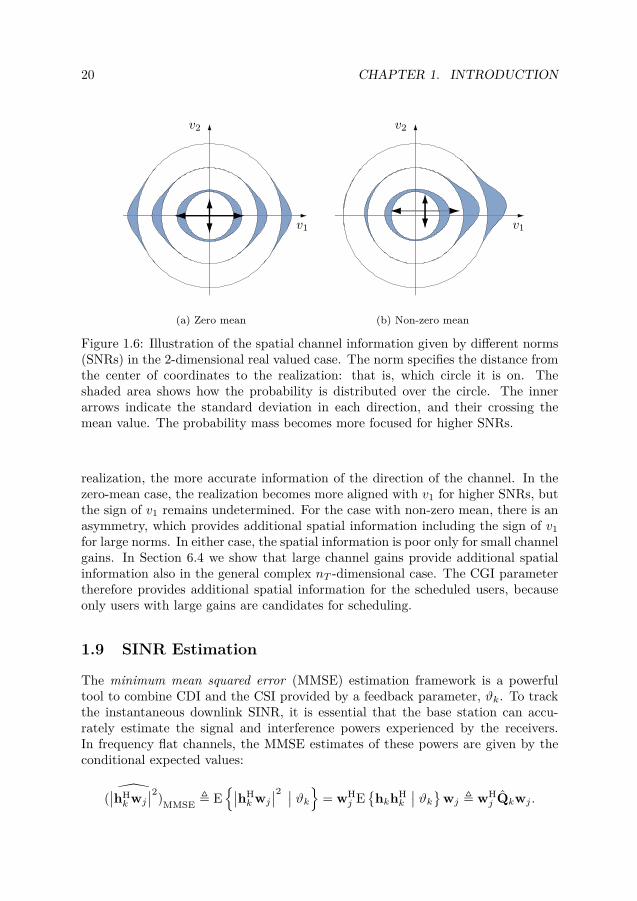
Figure 1.6 illustrates the joint conditional probability density function (PDF)of v1 and v2 for a given norm (instantaneous SNRs), ρ—the stronger the norm
20 CHAPTER 1. INTRODUCTION
v1
v2
(a) Zero mean
v1
v2
(b) Non-zero mean
Figure 1.6: Illustration of the spatial channel information given by different norms(SNRs) in the 2-dimensional real valued case. The norm specifies the distance fromthe center of coordinates to the realization: that is, which circle it is on. Theshaded area shows how the probability is distributed over the circle. The innerarrows indicate the standard deviation in each direction, and their crossing themean value. The probability mass becomes more focused for higher SNRs.
realization, the more accurate information of the direction of the channel. In thezero-mean case, the realization becomes more aligned with v1 for higher SNRs, butthe sign of v1 remains undetermined. For the case with non-zero mean, there is anasymmetry, which provides additional spatial information including the sign of v1for large norms. In either case, the spatial information is poor only for small channelgains. In Section 6.4 we show that large channel gains provide additional spatialinformation also in the general complex nT -dimensional case. The CGI parametertherefore provides additional spatial information for the scheduled users, becauseonly users with large gains are candidates for scheduling.
1.9 SINR Estimation
The minimum mean squared error (MMSE) estimation framework is a powerfultool to combine CDI and the CSI provided by a feedback parameter, ϑk. To trackthe instantaneous downlink SINR, it is essential that the base station can accu-rately estimate the signal and interference powers experienced by the receivers.In frequency flat channels, the MMSE estimates of these powers are given by theconditional expected values:
(∣∣hHkwj
∣∣2)MMSE � E{∣∣hH
kwj∣∣2 ∣∣ ϑk} = wH
j E{
hkhHk
∣∣ ϑk}wj � wHj Qkwj .
1.10. OUTLINE AND CONTRIBUTIONS 21
The instantaneous SINR in (1.9) can thus be estimated as
SINRk = wHk Qkwk∑
j �=kwHj Qkwj + σ2
k
.
Computing Qk � E{
hkhHk
∣∣ ϑk} is, however, in general non-trivial. A major con-tribution of this thesis is the development of efficient algorithms for computing Qkfor the CGI feedback parameters, ρk = ‖hk‖2, and ζk = ‖Akhk‖2.
1.10 Outline and Contributions
The focus of this thesis is resource allocation in multiuser multi-antenna digitalcommunication systems. The first part of the thesis deals with optimal beam-former optimization with additional side constraints. In Chapter 2, the theoreticalimplications of these additional constraints are analyzed and efficient optimizationalgorithms are established. We next demonstrate the usefulness of the proposedside constraints in Chapter 3, where they are used for several different applications.
Chapter 4 addresses the user selection problem. Here the partial CSI thatis provided by limited feedback is merged with CDI at the transmitter using anMMSE SINR estimation framework. These estimates enable efficient utilization ofmultiuser diversity and robust spatial separation of users.
In Chapter 5, we consider several suboptimal beamforming algorithms with lowcomputational complexity—well suited for the SINR expressions provided by theMMSE SINR estimation framework. These algorithms enable a computationallytractable implementation of the proposed user selection procedure.
In Chapter 6, we consider the limited feedback of a single scalar CGI parameterper user. We show how to efficiently apply the MMSE SINR estimation frameworkfor this choice of feedback parameter. The system performance of the proposeduser selection procedures and beamforming techniques, with such limited feedback,is demonstrated in Chapter 7.
In Chapter 8, we show how to use a broader class of CGI parameters. Theextended CGI framework can be used to significantly reduce the pilot signaling.The same framework also provides the tool for an approximation that significantlyreduces the computational complexity of computing the MMSE estimates for CGIfeedback. We conclude the thesis in Chapter 9.
Below we describe in more detail the contributions made in each chapter.
Chapter 2 – Optimal Beamforming with Side Constraints
Optimal beamforming has received much attention in the past few years [RFLT98,SB04, BS02, BO01]. The non-convex power minimization problem, subject to SINRQoS constraints, was first solved in [RFLT98] using the elegant virtual-uplink du-ality theory. An efficient and globally convergent algorithm, which also detects

22 CHAPTER 1. INTRODUCTION
infeasible scenarios, was later proposed in [SB04] using an approach similar to thatof [RFLT98]. In the same work, the related problem of maximizing the minimumSINR, subject to a power constraint is also considered and solved.
A fundamentally different approach for solving the power minimization problemwas proposed in [BO99, BO01], where the globally optimal solution is shown tocoincide with the optimum of a semidefinite relaxation. The semidefinite relaxationis a convex optimization problem, which can be solved using standard semidefiniteprogramming tools (e.g., SeDuMi [Stu99]).
In Chapter 2, we generalize these algorithms to cope with an additional con-straint on each beamformer. The extensions of both the semidefinite programmingapproach of [BO01] and the specialized algorithms of [SB04] are considered. Theframework enables additional constraints on the beamformer, wk, of the form
wHkAkwk ≥ wH
kBkwk,
or equality constraintswHkAkwk = wH
kBkwk,
where Ak and Bk are positive semidefinite (PSD) design matrices. By constructingthese matrices appropriately, the beamformers can be enforced to satisfy somedesired property. These constraints are inherently non-convex, and are referred toas indefinite shaping constraints. Their name emphasizes that they can be expressedin terms of the indefinite Hermitian matrix Ck � Ak −Bk as
wHkCkwk ≥ 0,
and similarly for equality constraints.We prove strong duality [BV04] of the beamforming problem with additional in-
definite shaping constraints; this guarantees that the optimal point of the semidef-inite relaxation coincides with that of the original beamforming problem. Theadditional constraints also affect the specialized algorithms of [SB04] and one ofthe subproblems becomes non-convex. By proving strong duality for this subprob-lem, we can use the convex dual problem [BV04] to efficiently solve the originalsubproblem.
The weighted sum-rate maximization problem is also considered in this chapter.Unlike the case with the power minimization and the SINR maximization formula-tions, the convergence to the global optimum of the weighted sum-rate maximiza-tion cannot be guaranteed. However, a reformulation of the problem is proposedthat significantly reduces the number of unstructured optimization variables.
The work in this chapter has been published in
[HBO03] D. Samuelsson (Hammarwall), M. Bengtsson, and B. Ottersten. Op-timal downlink beamforming with additional constraints. In Proceedings ofAsilomar Conference on Signals, Systems and Computers, November 2003.

1.10. OUTLINE AND CONTRIBUTIONS 23
[HBO05a] D. Samuelsson (Hammarwall), M. Bengtsson, and B. Ottersten. Anefficient algorithm for solving the downlink beamforming problem with in-definite constraints. In Proceedings of IEEE International Conference onAcoustics, Speech, and Signal Processing (ICASSP), March 2005.
[HBO06] D. Hammarwall, M. Bengtsson, and B. Ottersten. On downlink beam-forming with indefinite shaping constraints. IEEE Transactions on SignalProcessing, 54(9):3566–3580, September 2006.
[HBO07b] D. Hammarwall, M. Bengtsson, and B. Ottersten. Beamforming anduser selection in SDMA systems utilizing channel statistics and instantaneousSNR feedback. In Proceedings of IEEE International Conference on Acous-tics, Speech, and Signal Processing (ICASSP), April 2007.
Chapter 3 – Applications for Constrained Beamforming
In this chapter, we demonstrate several applications where indefinite shaping con-straints arise. We show how to formulate diversity constraints in DS-CDMA sys-tems, to ensure a minimum level of path diversity. Numerical evaluations showthat the robustness (i.e., the variance) of the SINR in the RAKE combined signalis improved.
Several interference constraints are also considered. One such interference appli-cation is relaxed nulling, where the interference to a specific user (in a neighboringcell) is limited to a fraction of the worst case interference. Using traditional beam-forming algorithms, only the special case of zero interference can be handled. It isdemonstrated that allowing a small limited interference yields significant gains interms of number of users that can be assigned simultaneously.
The work in this chapter has been published in [HBO06].
Chapter 4 – User Selection with MMSE SINR Estimation
In the previous chapters, the beamforming problem for a given set of assigned(selected) users has been considered. In best-effort systems with channel dependentscheduling, selecting a spatially compatible set of users is a dynamic process thatshould adapt to the current channel conditions. This user selection is the focus ofthis chapter. A generic MMSE SINR estimation framework is established, whichlets the transmitter estimate the instantaneous SINRs of all users, by utilizingall available feedback information. Robustness to estimation errors in the SINRsis incorporated using the MSE of the estimates; this enables a dynamic back offmargin that is designed to achieve a target outage probability (i.e., the probabilityof overestimating the SINR).
Optimally choosing a set of users is computationally intractable in most scenar-ios. Instead a suboptimal greedy user selection algorithm is proposed, which relieson low complexity beamforming techniques. The user selection procedure is similar

24 CHAPTER 1. INTRODUCTION
to the scheme proposed in [DS05], but is adapted to better suit systems limited topartial CSI at the transmitter. The work in this chapter is to be published in
[HBO07c] D. Hammarwall, M. Bengtsson, and B. Ottersten. Utilizing the spatialinformation provided by channel norm feedback in SDMA systems. IEEETransactions on Signal Processing, May 2007. Submitted.
Chapter 5 – Low-Complexity BeamformingTo select a spatially compatible group of users, the selection process proposed inChapter 4 repeatedly solves beamforming problems; this is not computationallytractable with optimal beamforming algorithms. In Chapter 5, we propose sub-optimal beamforming techniques, with low computational complexity—suitable forthe SINR estimates produced by the MMSE estimation framework. A general-ized zero-forcing (GZF) technique is proposed, which can be seen as an extensionto traditional zero-forcing (ZF) beamforming. Zero-forcing beamforming is widelyadopted and has been demonstrated to yield excellent performance in multiuser sys-tems with perfect CSI [YG06]. In case of partial CSI, as considered in this thesis,ZF has several shortcomings that are addressed in the proposed GZF algorithm.The GZF algorithm preserves the low computational complexity of ZF and alsohas the desirable property that the beamformers are readily updated to admit anadditional user. This is particularly useful in the greedy user selection process.
Another beamforming algorithm is also proposed that is based on the minimumvariance distortionless response (MVDR) criterion [MM80]. By transforming thebeamforming problem to the virtual-uplink (VUL) domain [RFLT98, SB04], theMVDR optimal beamformers are obtained in closed form using standard matrixinversions. The VUL MVDR beamforming algorithms performs slightly betterthan the GZF algorithm, at the cost of increased computational complexity.
Modifications to the criteria of the two beamforming algorithms are also pro-posed that enable the computation of the beamformers from a single matrix inver-sion. These one-shot algorithms significantly reduce the computational complexityat the cost of a small performance degradation.
The work in this chapter is to be published in [HBO07c].
Chapter 6 – MMSE SINR Estimation with CGI FeedbackTo track the variations in the SINRs for scheduling and user selection purposes,the transmitter must have CGI. In Chapter 6, we consider a system where thetransmitter has only CDI and scalar CGI. Each user, k, feeds back the scalarchannel-gain parameter, ρk, which is taken as the squared Euclidean channel norm:
ρk � ‖hk‖2 .
The transmitter is thus limited to the channel information provided by ρk and thestatistics of the channel in the user selection and beamforming. CDI and CGI of

1.10. OUTLINE AND CONTRIBUTIONS 25
each user are merged using the MMSE SINR estimation framework proposed inChapter 4. To that end the conditional channel probability density function (PDF),
f(hk|ρk),
is derived, which provides the tools to compute the conditional moments requiredto for the SINR estimates.
The Rayleigh fading channel is given special attention, for which the conditionalPDF is derived in closed form. Also, the second and fourth order moments arederived in closed form; the SINR estimates and MSEs are thus readily computed.An asymptotic analysis is performed, which confirms the behavior demonstrated inFigure 1.6, also for the nT complex dimensional case; that is, the spatial channelinformation increases when ρk increases.
Also, the general Ricean fading case is considered. The asymmetry introducedby the non-zero mean does however prevent the derivation of closed form expres-sions. However, by means of Laplace transformation, the conditional PDFs andmoments can be expressed as a series of modified Bessel functions of the first kind.By truncating these relatively rapidly converging series, the conditional momentscan be efficiently computed.
The work in this chapter has been published in
[HBO05b] D. Samuelsson (Hammarwall), M. Bengtsson, and B. Ottersten. Im-proved multiuser diversity using smart antennas with limited feedback. InProceedings of European Signal Processing Conference (EUSIPCO), Septem-ber 2005.
[HO06a] D. Hammarwall and B. Ottersten. Exploiting the spatial informationprovided by channel statistics and SNR feedback. In Proceedings of IEEEInternational Workshop on Signal Processing Advances for Wireless Commu-nications (SPAWC), July 2006.
[HBO07a] D. Hammarwall, M. Bengtsson, and B. Ottersten. Acquiring partialCSI for spatially selective transmission by instantaneous channel norm feed-back. IEEE Transactions on Signal Processing, June 2007. Accepted forpublication.
Chapter 7 – Performance EvaluationCombining the user selection algorithm of Chapter 4 and the low complexity beam-forming algorithms of Chapter 5, with the analytical results of Chapter 6, providesthe tools to utilize a limited CGI feedback for channel dependent user selectionand beamforming using MMSE SINR estimation. In Chapter 7, the performanceof such an SDMA system is demonstrated in a wide-area scenario.
We compare the performance of the different low complexity beamforming al-gorithms proposed in Chapter 5. Numerical evaluations show that the performance
26 CHAPTER 1. INTRODUCTION
achieved by VUL MVDR beamforming cannot be notably increased by post op-timization of the beamformers and power allocation using the weighted sum-ratecriterion, as proposed in Chapter 2. This indicates that when VUL MVDR beam-forming is combined with user selection, it achieves near optimal performance.
As expected, GZF and the one-shot versions have a small performance losscompared to VUL MVDR beamforming, but this loss may be well motivated by thecomputational complexity advantages. The system performance is also compared toother schemes based on CGI feedback, and the MMSE SINR estimation frameworkis shown to outperform these methods in most scenarios.
A finite rate feedback scheme is also proposed, which limits the feedback res-olution of ρk to b bits/user. Simulations demonstrate that the performance losswith finite rate feedback is limited, and a significant fraction of the throughput ofknowing ρk perfectly is achieved with b = 1 bits/user.
Parts of the work in this chapter are to be published in [HBO07c].
Chapter 8 – Generalization of the CGI ParameterIn some cases, the CGI feedback parameter, ‖hk‖2, may be unsuitable. For instancein order to accurately estimate ‖hk‖2 all nT complex dimensions of the channel,hk, must be excited. This results in significant pilot signaling overhead, especiallyin multi-cell systems where the pilot signals of neighboring cells often are requiredto be orthogonal.
In Chapter 8, the generalized CGI feedback parameter,
ζk � ‖Akhk‖2 ,is considered, where Ak is an arbitrarily chosen matrix. The conditional channelmoments required by the MMSE SINR estimation framework are derived.
This generalized CGI parameter can be used to resolve the pilot signaling over-head. If only a subset of the antennas are excited in the pilot signaling, the userterminals could still estimate ζk if Ak is chosen such that only the correspondingelements are non zero. The transmitter can next combine ζk with the statistics ofthe full channel vector, and use all antenna elements in the data transmission.
Numerical simulations, for the wide-area scenario, demonstrate that, for systemwith eight transmit antennas, it is sufficient to excite four elements in the pilotsignaling to achieve the full performance, and only a small performance loss resultswith pilot signaling limited to two antennas.
We also show how to use the framework with generalized CGI parameter tosignificantly reduce the computational complexity of computing the MMSE SINRestimates; this is achieved by introducing an approximation that is suitable forlarge realizations of ζk.
Parts of the work in this chapter have been published in
[HO06b] D. Hammarwall and B. Ottersten. Spatial transmit processing usinglong-term channel statistcs and pilot signaling on selected antennas. In Pro-

1.11. CONTRIBUTIONS OUTSIDE THE SCOPE OF THE THESIS 27
ceedings of Asilomar Conference on Signals, Systems and Computers, October2006.
and have been submitted in [HBO07c].
1.11 Contributions Outside the Scope of the Thesis
MIMO test-bed implementationTo demonstrate the potentials of MIMO systems a real-time 2 by 2 MIMO systemoperating in the 1800MHz range was implemented in an indoor non-line-of-sightenvironment using off-the-shelf radio hardware. Spatial multiplexing [RC98] wasused to achieve spectral efficiencies up to 15 bits/s/Hz. It was shown that thedeficiencies of the relatively simple hardware could be overcome using advancedsignal processing techniques.
This work was published in
[ZJL+04] P. Zetterberg, J. Jaldén, H. Lundin, D. Samuelsson (Hammarwall),P. Svedman, and X. Zhang. Implementation of SM and rxtxIR on a DSP-based wireless MIMO test-bed. In The European DSP Education and Re-search Symposium EDERS, November 2004.
[HJZO06] D. Samuelsson (Hammarwall), J. Jaldén, P. Zetterberg, and B. Otter-sten. Realization of a spatially multiplexed MIMO system. EURASIP Jour-nal on Applied Signal Processing, 2006:Article ID 78349, 16 pages, February2006.
Subcarrier SNR estimation at the transmitter for reducedfeedback in OFDMA systemsIn OFDMA systems with channel dependent scheduling, it is essential to keep trackof the SNR on each subcarrier, for all the users. In systems with many users, andmany (hundreds or even thousands) of subcarriers, this can result in unrealisticfeedback overhead if the user terminals are to feedback all these SNRs.
In this work, a method to significantly reduce this overhead is proposed. Insteadof feeding back every subcarrier SNR, only subcarriers on a sparse, evenly spaced,grid are considered for feedback. In addition, only the highest SNRs on this gridare fed back.
Hence only a small subset of the subcarrier SNRs is made available to thetransmitter. Using the correlation among the subcarrier SNRs, the transmitterestimates the SNRs on the intermediate subcarriers; this technique is demonstratedto result in only a small performance losses compared to knowing all SNRs perfectly.The MMSE estimate of an intermediate subcarrier SNR is derived in closed form,and shown to outperform other estimation techniques. The work has been publishedin

28 CHAPTER 1. INTRODUCTION
[SHO06] P. Svedman, D. Hammarwall, and B. Ottersten. Sub-carrier SNR esti-mation at the transmitter for reduced feedback OFDMA. In Proceedings ofEuropean Signal Processing Conference (EUSIPCO), September 2006.
Capacity achieving transmit strategies with CGI at thetransmitterThe ergodic capacity of a MIMO link is greatly affected by the CSI available atthe transmitter. In this work, the ergodic capacity achieving transmit strategy fora MIMO system with CGI feedback is derived and analyzed. Special attentionis given to the beamforming optimality range (i.e., the range where single-streambeamforming is optimal). It is observed that beamforming is capacity achieving forsufficiently large channel gain, ρ = ‖h‖2. The work has been published in
[JHO07] E. Jorswieck, D. Hammarwall, and B. Ottersten. Ergodic capacityachieving transmit strategy in MIMO systems with statistical and short-termnorm CSI. In Proceedings of IEEE International Conference on Acoustics,Speech, and Signal Processing (ICASSP), April 2007.
CGI feedback in systems with multiple receive antennasIn this thesis, only the case of a single receive antenna at each user terminal isconsidered. In this work, the MMSE SINR estimation framework is extended tofacilitate some CGI parameters for the general multiple-input multiple-output case.The work has been published in
[BHO07] E. Björnson, D. Hammarwall, and B. Ottersten. Beamforming utilizingchannel norm feedback in multiuser MIMO systems. In Proceedings of IEEEInternational Workshop on Signal Processing Advances for Wireless Commu-nications (SPAWC), June 2007.

Chapter 2
Optimal Beamforming with SideConstraints
A system with an antenna array at the base station, can exploit the spatial charac-teristics of the wireless channel (e.g., using beamforming). In this chapter we con-sider beamformer optimization for the downlink of a wireless network. A downlinkbeamformer shapes the radiation patterns and thereby amplifies the desired signal,and more importantly, limits interference to co-channel users. Such beamforming—implemented as a linear precoder—enables simultaneous scheduling of several usesseparated in space (i.e., SDMA).
In this chapter, we consider optimized beamforming and extend available al-gorithms to enable a class of indefinite quadratic side constraints. We prove thatstrong duality is preserved for this class of additional constraints, which allows theoptimization problem, in line with [BO99, BO01], to be formulated as a convexsemidefinite program, which can be efficiently solved using standard convex opti-mization [BV04]. We also generalize the more specialized algorithms proposed in[SB04] to cope with the proposed class of additional constraints.
In previous optimal downlink beamforming literature, the SINR expression hasbeen quite limited in its structure, which can lead to difficulties when more involvedscenarios are considered—for example, CDMA systems with non-zero self interfer-ence. Therefore we consider a more general form of the SINR expression and extendprevious results in downlink beamforming to the generalized SINR expression.
2.1 Introduction to Optimal Beamforming
Several downlink SDMA schemes have been proposed in the literature. Suboptimal,low complexity schemes were initially proposed—including the zero forcing spatialequalizer [GP94] and the harmonic mean SINR maximization considered in [Zet97].In this section, we focus on two formulations of optimal downlink beamforming (andpower control): the minimization of the total transmission power in the system,
29

30 CHAPTER 2. OPTIMAL BEAMFORMING WITH SIDE CONSTRAINTS
subject to an individual QoS constraint for each user; and the maximization ofthe weakest QoS, subject to a sum-power constraint. We also briefly discuss theweighted sum-rate problem.
Minimizing the transmission power in a system is motivated by many factors;for example, it minimizes the interference to neighboring cells, and the amplifiers atthe transmitter have a limited power range. The power-minimization formulation ofthe beamforming problem was originally formulated and solved in [RFLT98], usingSINR as the QoS measure. An iterative algorithm was proposed, which finds theglobal optimum. The algorithm is based on the elegant virtual-uplink duality con-cept; that is, the optimal downlink beamformers are computed from a less involvedvirtual-uplink formulation. A similar but more stable and rapidly converging algo-rithm for optimal downlink beamforming, which also detects infeasible scenarios,was later proposed in [SB04], and further analyzed and generalized in [BS05], wherea unified framework was presented. The alternative formulation which maximizesthe QoS, subject to a total transmission power constraint, was also formulated andsolved in [SB04], using SINR as QoS.
A different approach of solving the optimal beamforming problem was intro-duced in [BO99], where the authors attack the problem using semidefinite opti-mization. It was shown how an optimal solution can be obtained from the convex,readily solvable, semidefinite relaxation [BV04].
These algorithms for optimal downlink beamforming are however all limitedto SINR as QoS measure; this limitation excludes many other factors that affectthe performance of a communication link—such as, physical limitations, diversityaspects, and interference requirements—that should be taken into consideration inthe optimization. The limitations of only using SINR as QoS measure motivate theintroduction of side constraints on the beamformers (linear precoders). A varietyof such constraints are considered in [BO99, BO01], which suggest how to solvethe constrained optimization, using semidefinite optimization. The semidefiniteprogramming approach does however only ensure an optimal solution, when strongduality [BV04] holds for the considered downlink beamforming problem. For theoptimal downlink beamforming problem, without side constraints, strong dualitywas proved in [BO01].
2.2 Problem Formulation
In this section, the downlink beamforming problem is formulated and analyzed. Theoptimization problem has many useful inherent properties, which are presented andelaborated upon.
The beamforming optimization is performed with respect to the SINRs, whichin line with Chapter 1.4 are modeled as
SINRk = wHkRdesk wk
wHkRSIk wk +
∑j∈S\{k}wH
j RMAIkj wj + σ2
k
, k ∈ S, (2.1)

2.2. PROBLEM FORMULATION 31
where S are the scheduled (selected) users, σ2k is the AWGN power, and the pos-
itive semidefinite (PSD) matrices Rdesk , RSI
k and RMAIkj represent the desired, self
interfering, and multi-access interfering power, respectively.The SINR expression (2.1) is general in its form and accurately models the SINR
in most systems. In Appendix C.2 a DS-CDMA system model is presented and thelong-term SINR of the maximum ratio combined (MRC) signal of a RAKE receiveris shown to be well approximated by an expression of the desired form.
The beamformer notation, wk, incorporates both beamforming direction andpower allocation, but it is often useful separate these as wk = √pkuk, wherepk � ‖wk‖2 and ‖uk‖ = 1. Both representations are used in the sequel. Withoutloss of generality, we disregard all users that are not scheduled (or assigned) andlet S be the complete set of users,
S = {1, 2, . . . ,K}.Also, for notational convenience the beamformers are collected in the matrix,
U = [u1 . . .uK ],
and the powers are collected in the vector,
p = [p1 . . . pK ]T,
where {·}T denotes the transpose operator.
Indefinite shaping constraintsThe primary objective of downlink beamforming has traditionally only been toensure that each user meets an individual target SINR, γi. However, there aremany applications for which each beamformer, wi, in addition should satisfy anindefinite quadratic inequality/equality constraint of the form,
wHkCkwk = 0 ∀k ∈ E ,
wHkCkwk ≥ 0 ∀k ∈ E ,
where E is the set of users with equality constraints. The indefinite (Hermitian)matrices Ck are design parameters and can be chosen arbitrarily to formulate manytypes of constraints. For notational convenience, we define the set
U �
⎧⎨⎩U
∣∣∣∣∣∣uHkCkuk = 0 ∀k ∈ E ,
uHkCkuk ≥ 0 ∀k ∈ E ,‖uk‖ = 1 ∀k,
⎫⎬⎭ (2.2)
to denote the set of U that satisfy the indefinite constraints.In Chapter 3, we suggest several applications where indefinite constraints arise,
including different interference constraints and path-diversity constraints for DS-CDMA systems.

32 CHAPTER 2. OPTIMAL BEAMFORMING WITH SIDE CONSTRAINTS
As mentioned above, the quadratic indefinite constraints, U ∈ U , can be chosenso as to formulate various kinds of constraints. Any indefinite matrix C can bewritten in terms of PSD matrices C = A−B. The indefinite inequality (similarly forequality) constraints can thus equivalently be formulated as wH
kAkwk ≥ wHkBkwk.
This formulation gives more insight into the constraint. Typical, more or less useful,constraints of this form are
• At most a chosen fraction of the received signal power may come from theline-of-sight component.
• At most a chosen fraction of the power assigned to a user, may be emitted ina certain spatial direction.
• The MAI at user j caused by user k, is less than a chosen fraction of thesignal power received by user k.
• The beamformer wk must be confined to the null space of Bk. This corre-sponds to Ak = 0.
It should be pointed out that the quadratic indefinite constraints are indepen-dent of the scaling of wi. The power allocation p is therefore not affected explicitlyby the imposed constraints, but only implicitly through its dependence on thebeamformers, whereas the spatial characteristics U are limited by the constraints.Readers who want more intuition of the indefinite constraints may want to readabout the proposed applications in Chapter 3 prior to the sequel, which is of moretheoretical nature.
Formulation of the optimization problems
Herein, three different problem formulations are considered. The first formulationminimizes the total transmission power in the system, while meeting the individualSINR targets γk. Denoting the vector of all ones1 as 1, the transmission power isgiven by
∑k ‖wk‖2 = 1Tp, and the optimization problem, P , is formulated as
P �
⎧⎪⎪⎨⎪⎪⎩minU,p 1Tp,
s.t. SINRk(U,p) ≥ γk ∀k,p ≥ 0,U ∈ U ,
(2.3)
where 0 is the zero vector (or matrix) and ≥ is element-wise inequality. This power-minimization problem, P , is useful because it provides a power efficient system,which consequently leaks little power to neighboring cells in terms of inter-cellinterference. The second formulation, Γ , tries to maximize the system performance
1The size of 1 is implicitly determined from its use.

2.2. PROBLEM FORMULATION 33
in terms of user throughput, by maximizing the minimum normalized downlinkSINR
SINRmin � mink
SINRkγk,
given a total power constraint, Pmax. Here, γk are interpreted as QoS weights forthe different users. In summary,
Γ(Pmax) �
⎧⎪⎪⎨⎪⎪⎩maxU,p SINRmin(U,p)
s.t. 1Tp ≤ Pmax,p ≥ 0,U ∈ U ,
(2.4)
where the notation Γ(Pmax) is used to explicitly state the dependence on Pmax.This second formulation, Γ , is also useful for testing feasibility and finding initialfeasible points of P . This is because Γ is always feasible (unless some Ck is negativedefinite) and because P is feasible if and only if the optimal value of Γ , valΓ , isgreater or equal to 1 for some maximum power, Pmax:
∃P, valΓ(P ) ≥ 1⇐⇒ ∃ p ≥ 0,U ∈ U , with SINRk ≥ γk ∀k⇐⇒ P feasible.
The third optimization problem of interest is the weighted sum-rate maximiza-tion
RΣ(Pmax) �
⎧⎪⎪⎨⎪⎪⎩maxU,p
∑k βkR
(SINRk(U,p)
)s.t. 1Tp ≤ Pmax,
p ≥ 0,U ∈ U ,
(2.5)
where βk ≥ 0 is the priority, or weight, of user k. RΣ is a more difficult problemthan the other formulations, and contrary to P and Γ , convergence to the globaloptimum cannot be guaranteed.
Properties of the optimal pointsThe SINR constraints of P can be compactly written in matrix form by introducingthe matrix
D(U) = diag{
γ1uH
1 Rdes1 u1
, . . . ,γK
uHKRdes
K uK
}and the cross-talk matrix
[Ψ(U)]kj ={
uHj RMAIkj uj j = k,
uHkRSIk uk j = k,
where diag {. . .} is a diagonal matrix with the indicated diagonal elements and[·]kj denotes the element on the kth row, and jth column of a matrix. The SINRconstraints can now, using (2.1), be written as(
I−DΨ)p ≥ Dσ,

34 CHAPTER 2. OPTIMAL BEAMFORMING WITH SIDE CONSTRAINTS
where σ = [σ21 , . . . , σ
2K ]T.
SINRk(U,p) is strictly monotonically increasing2 in pk and monotonically de-creasing in pj , j = k, therefore the SINR constraints of P are always (when fea-sible) met with equality: Otherwise pk could be decreased without violating anyconstraints, contradicting the optimality. Hence for a given U0, the associatedoptimal power distribution p� can be solved from the linear system of equations(
I−DΨ)p� = Dσ. (2.6)
Similarly, at the optimal point of Γ the SINRs are balanced as
Γ = SINRmin = SINR1
γ1= · · · = SINRK
γK, (2.7)
and Γ is therefore referred to as the SINR balancing problem. For a given U0, theoptimal power distribution p�—that maximizes SINRmin—has been shown [YX98,SB04] to be given by the eigenvalue problem
Υ(U0,Pmax)pext = λmaxpext, pext =[p�1
](2.8)
where pext is the, properly scaled, positive eigenvector associated with the maxi-mum eigenvalue λmax of the extended downlink coupling matrix
Υ(U,Pmax) �[
DΨ Dσ1
Pmax1TDΨ 1
Pmax1TDσ
]. (2.9)
The balanced normalized SINR level is obtained as
Γ = SINRmin = 1λmax.
Even though only the case without self interference (i.e., RSIi = 0) was considered in
[YX98, SB04], the result generalizes straightforwardly to non-zero self interference.For a given U0, and known optimal SINR balancing level, Γ� = Γ�(U0), (2.7) maybe written in a form similar to (2.6) as
( 1Γ� I−DΨ
)p� = Dσ, (2.10)
from which we can solve for the downlink power allocation, p�, that is optimal forthe given beamformers, U0.
2We assume (U,p) to be in the feasible set and that γk > 0 (i.e., uHkRdesk uk > 0).

2.2. PROBLEM FORMULATION 35
Relations between P, Γ and RΣ
The two formulations P and Γ are closely related, and if the power constraintPmax of Γ is set to the optimal minimum power, valP , they are equivalent in thesense that they have the same set of globally optimal points, argΓ(valP) = argP[SB04], where arg{·} denotes the set of optimal points. This follows because anyoptimal solution results in the same set of SINRs, as stated by (2.6) and (2.7). Inparticular, P can be formulated in terms of Γ as
P ⇐⇒{
minP P,s.t. valΓ(P ) ≥ 1. (2.11)
Conversely, Γ can be formulated in terms of P as
Γ ⇐⇒{
maxΓ Γ,s.t. valP(Γγ1, . . . ,ΓγK) ≤ Pmax,
(2.12)
where the notationP(Γγ1, . . . ,ΓγK) is used to explicitly state that the optimizationis with respect to the SINR targets γk = Γγk. The optimization problem, Γ , cantherefore readily be solved using any solver of P , because valP(Γγ1, . . . ,ΓγK) is astrictly monotonically increasing function of Γ.
Similarly the weighted sum-rate problem, RΣ, can be expressed in terms of Γas
RΣ ⇐⇒{
maxγ
∑k βkR
(γkvalΓ(γ)
)s.t. 1Tγ = 1, γ ≥ 0, (2.13)
where the vector γ collects the scalars, γk ∀k, and the notation Γ(γ) is usedto emphasize the dependence on γ. To see this, note that the SINRs may beparameterized in terms of γ and Γ as
SINRk = Γγk ∀k, where1Tγ = 1,γ ≥ 0,Γ ≥ 0.
where the normalization of γ resolves the scaling ambiguity between Γ and γ. Forfixed γ, all SINRs are increasing with Γ, which is upper bounded as Γ ≤ valΓ(γ)according to (2.7). The formulation in (2.13) follows, because the rate function,R(·), is assumed to be non-decreasing. The maximization in (2.13) does howeverremain non-convex, but the number of optimization parameters is substantiallyreduced.
Uplink–downlink duality
The concept of uplink–downlink duality was first introduced in the beamformingcommunity in [RFLT98] and later more rigorously analyzed in [BS02] and [SB04].
36 CHAPTER 2. OPTIMAL BEAMFORMING WITH SIDE CONSTRAINTS
Related results were also derived in [TV02] and [BO01]. The uplink–downlinkduality motivates the introduction of the virtual-uplink SINR
SINRVULk (uk,q) = qkuH
kRdesk uk
uHk
(qkRSI
k +∑j �=k qjRMAI
jk + I)
uk, (2.14)
where qk are the virtual-uplink power allocations3, which are collected in the vectorq = [q1, . . . , qK ]T. Note the indices of RMAI
jk , which are interchanged compared tothe downlink SINR. In matrix form the virtual-uplink SINR constraints SINRVUL
k ≥γk can be written as (
I−DΨT(U))q ≥ D1
and SINRVULmin (U,q) is defined analogously to SINRmin(U,p) for the downlink.
The virtual uplink is more simple to analyze than the downlink because the uplinkbeamformers are coupled only through q, contrary to the downlink SINRs in (2.1),which are also coupled through U. Hence, the following result is useful.
Theorem 2.1. For any given U0 and Pmax it holds that
maxp:1Tp≤Pmax
SINRmin(U0,p) = maxq:σTq≤Pmax
SINRVULmin (U0,q).
Proof. The proof is given in [SB04], which to a large extent relies on the results in[BS02]. The given proof considers the case without self interference, i.e. RSI
k = 0,but the result generalizes straightforwardly to non-zero self interference.
Theorem 2.1 reduces the complexity of the downlink problem to that of theuplink, because it states that the virtual-uplink problem may be solved insteadof the downlink problem. Also note that the virtual uplink is constrained by aweighted power constraint σTq ≤ Pmax, which affects the optimization slightly.The virtual-uplink reformulation of Γ is given by
ΓVUL �
⎧⎪⎪⎨⎪⎪⎩maxU,q SINRVUL
min (U,q)s.t. σTq ≤ Pmax,
q ≥ 0,U ∈ U .
(2.15)
It follows from Theorem 2.1 that Γ and ΓVUL attain the same optimal value andthat any optimal U� with respect to one problem, is also optimal with respect tothe other,
valΓ = valΓVUL, argUΓ = argUΓVUL,
3Note the notational difference to [SB04] where the normalized matrices, Rdesk = σ−2
kRdesk and
RMAIkj = σ−2
kRMAIkj , are introduced (self interference is not considered), and the corresponding
normalized virtual-uplink powers, qk = σ2kqk, are used in place of q. In the following such a
variable change is not appropriate, because q has a nice relation to the dual optimization problemintroduced in Section 2.3.

2.3. BEAMFORMING USING SEMIDEFINITE PROGRAMMING 37
where the notation argU{·} is used to denote the set of globally optimal U of anoptimization problem. The optimal power allocation p� of Γ is readily obtainedfrom U� using (2.8), or by solving (2.6) using the SINR targets γk = γk · valΓVUL.We thus have the following corollary:
Corollary 2.2. The SINR balancing problem Γ is algebraically equivalent to thevirtual-uplink SINR balancing problem ΓVUL, attaining the same optimal value.Further, the same U� is optimal with respect to both problems.
Similarly, the virtual-uplink reformulation of the power-minimization problemP is given by
PVUL �
⎧⎪⎪⎨⎪⎪⎩minU,q σTq
s.t. SINRVULk (uk,q) ≥ γk ∀k,
q ≥ 0,U ∈ U .
(2.16)
By using Corollary 2.2, and that P and PVUL can be equivalently written in termsof Γ and ΓVUL, respectively, as in (2.11), it follows that
valP = valPVUL, argUP = argUPVUL,
and the optimal power allocation, p�, of P can be obtained from the optimal U�using (2.6). The preceding discussion proves the following corollary:
Corollary 2.3. The power-minimization problem P is algebraically equivalent tothe virtual-uplink power-minimization problem PVUL, attaining the same optimalvalue. Further, the same U� is optimal with respect to both problems.
2.3 Beamforming Using Semidefinite Programming
In this section, we show that the power-minimization problem, P , can be solvedusing semidefinite programming. We prove that the globally optimal point may beobtained from a convex, readily solvable semidefinite relaxation of P . Bengtssonand Ottersten [BO99] showed how to rewrite the unconstrained downlink power-minimization problem as a semidefinite program. Next, the same approach is usedbut we take the indefinite shaping constraints into account. The SINR constraints,SINRk ≥ γk, can be rewritten using (2.1) as
wHkRMSk wk −
∑j �=k
wHj RMAIkj wj − σ2
k ≥ 0, (2.17)
where the modified signal covariance is defined as
RMSk � 1
γkRdesk −RSI
k .

38 CHAPTER 2. OPTIMAL BEAMFORMING WITH SIDE CONSTRAINTS
By introducing the PSD matrices, Wk = wkwHk ∀k, and applying the relation,
wHkRwk = Tr {RWk} ,
which follows from (B.1) in Appendix B, the semidefinite relaxation of P , SP , isobtained as
SP �
⎧⎪⎪⎪⎪⎪⎪⎪⎪⎨⎪⎪⎪⎪⎪⎪⎪⎪⎩
minWk
∑k Tr {Wk} ,
s.t. Tr{
RMSk Wk
}− ∑j �=k
Tr{
RMAIkj Wj
}− σ2k ≥ 0 ∀k,
Tr {CkWk} = 0 k ∈ E ,Tr {CkWk} ≥ 0 k ∈ E ,Wk = WH
k � 0 ∀k,
(2.18)
where A � B denotes that A−B is PSD. If in addition, Wk ∀k, are required to berank one, the semidefinite formulation would be equivalent to P . The semidefiniterelaxation, SP , is a convex semidefinite program and is typically solved using aprimal-dual interior point method, for which there are several standard optimiza-tion tools (e.g., SeDuMi [Stu99]). The primal-dual solvers readily detect infeasiblescenarios and the computed value of the criterion function can be guaranteed to bewithin a specified distance to the optimal value.
By dropping the rank one constraints, the optimization problem is relaxed andthe optimal value of SP is thus less or equal to that of P ,
valSP ≤ valP . (2.19)
Of particular interest is the special case when the optimal value of SP coincideswith that of P : Then there exists an optimal point, W�
k, of SP that is rank onefor all k (i.e., W�
k = wkwHk ∀k). In this case, wk, is also an optimal solution to P .
In the following we show, by using the special structure of P , that the inequality(2.19) is always satisfied with equality. The optimal point of P can thus always beobtained from the readily solvable semidefinite relaxation, SP .
The dual problem of PThe Lagrange dual problem [BV04] of both P and SP can be written as
DP �
⎧⎪⎪⎪⎪⎪⎨⎪⎪⎪⎪⎪⎩
maxU,q
σTq,
s.t. I− qkRMSk +
∑j �=kqjRMAI
jk − μkCk � 0 ∀k,q ≥ 0,μk ≥ 0 k ∈ E ,
(2.20)
where μk are the Lagrange multipliers for the indefinite shaping constraints, and qkare the Lagrange multipliers of the SINR constraints, as formulated in (2.17) (i.e.,

2.4. BEAMFORMING USING THE VIRTUAL-UPLINK DOMAIN 39
qk is the sensitivity of a change in σ2k). Interestingly, the Lagrange multipliers, qk,
coincide with the virtual-uplink powers. By weak duality4 the inequality (2.19) canbe extended as
valDP ≤ valSP ≤ valP . (2.21)
Strong duality of PTo prove that SP always attains the same value as P , we prove strong duality[BV04] for P ; that is, the Lagrange dual problem, DP , obtains the same optimalvalue as P .
Theorem 2.4. Strong duality holds for the power-minimization problem P; thatis,
valDP = valSP = valP .
Proof. The proof relies on Lemma 2.10 in Appendix 2.A, which states that for thepower-minimization problem it holds that valP ≤ valDP . This combined with theinequality in (2.21) results in valDP = valSP = valP .
The special characteristics of P thus ensure that (2.21) is satisfied with equality,and the next corollary is an immediate consequence of this result.
Corollary 2.5. The semidefinite relaxation, SP, always has at least one optimalsolution where all Wk are rank one5.
Hence, the globally optimal solution to the non-convex power-minimizationproblem, P , is always obtained from the solution of the readily solvable, convexsemidefinite relaxation SP .
2.4 Beamforming Using the Virtual-Uplink Domain
In this section, two specialized algorithms, solving the indefinitely constrainedpower-minimization problem P and the SINR balancing problem Γ , respectively,are presented. The algorithms are extensions of those presented in [SB04], whichhandle only the unconstrained case. These algorithms take advantage of the specialstructure of the problem and efficiently exploit the benefits of the virtual-uplink du-ality. The algorithms first solve the associated virtual-uplink problem, from whichthe optimal downlink beamformers are obtained and the optimal downlink power
4SP satisfies Slater’s refined conditions [BV04], because all constraints of SP are affine inWk. Thus, strong duality actually holds for SP.
5The case when one or several Wk are not rank one, corresponds to non-unique solutions toP. This occurs only when there is perfect symmetry in the problem, which is never the case inpractice. However, the optimal point wk of P is in the range of the high rank Wk and can beobtained using a similar approach as used in the proof of Lemma 2.10.

40 CHAPTER 2. OPTIMAL BEAMFORMING WITH SIDE CONSTRAINTS
allocation can be computed from a linear system of equations; that is, for P , p� issolved from (2.6), and for Γ , p� is solved from the first K equations of (2.8), where
λmax = 1Γ = 1
SINRVULmin
is known.The main advantage of these specialized algorithms is the reduced computa-
tional complexity over the use of standard optimization tools for the semidefiniteformulations of Section 2.3. The implementation is straightforward and involves(generalized) eigenvalue problems for which computationally efficient algorithmsare widely available.
Algorithmic solutions to P and Γ are stated in Table 2.1. For unconstrainedbeamformers, the global convergence of these algorithms is proved in [SB04], but—as first observed in [HBO05a]—this result generalizes to the constrained case. Theglobal convergence with constrained beamformers can also readily be seen usingthe unified framework later presented in [BS05].
The algorithmic solutions in Table 2.1 to P and Γ , reduce the optimization totwo subproblems, which are easier to solve. Firstly, virtual-uplink power controlfor fixed beamformers, U0,
q�(U0,Pmax) = arg maxqTσ≤Pmax
SINRVULmin (U0,q), (2.22)
and secondly, uplink beamformer optimization for fixed power allocation, q0
U�(q0) = arg maxU∈U
SINRVULmin (U,q0). (2.23)
The global optimum of P and Γ are rapidly attained by iteratively alternatingbetween the two preceding problems.
Power controlThe optimal downlink and virtual-uplink power allocations, for a given set of fixedbeamformers U, remain unaffected by the introduction of shaping constraints. Theoptimal downlink power allocation, p�(U), is given by the eigenvalue problem (2.8)as stated in Section 2.2. Similarly, the solution to the virtual-uplink power alloca-tion, q�(U), is given [SB04] 6 by the eigenvalue problem
Λ(U,Pmax)qext = λmaxqext, qext =[
q�1
], (2.24)
where qext is the positive eigenvector associated with the maximum eigenvalue λmaxof the extended virtual-uplink coupling matrix
Λ(U,Pmax) �[
DΨT(U) D11
PmaxσTDΨT(U) 1
PmaxσTD1
]. (2.25)
6In [SB04] the power constraint 1Tq ≤ Pmax is used, but the extension to σTq ≤ Pmax istrivial with a change of variables.

2.4. BEAMFORMING USING THE VIRTUAL-UPLINK DOMAIN 41
(a) Solution of Γ1: q← 02: repeat3: U← U�(q)4: q← q�(U,Pmax)5: until |ΔΓ| ≤ ε6: p←
(1Γ I−DΨ(U)
)−1Dσ
(b) Solution of P1: q← 02: repeat3: U← U�(q)4: q← q�(U,Pmax)5: until Γ ≥ 16: U← U�(q)7: repeat8: q← (I−DΨT(U))−1D19: U← U�(q)
10: until SINRVULmax − SINRVUL
min ≤ ε11: p←
(I−DΨ(U)
)−1Dσ
Table 2.1: Algorithmic solutions to the SINR balancing problem, Γ , and the power-minimization problem, P . Here, Γ = SINRVUL
min = SINRVULk /γk = λ−1
max is thebalanced virtual-uplink SINR, as obtained in the virtual-uplink power optimization,ΔΓ denotes the difference in two consecutive iterations and SINRVUL
max , denotes themaximum normalized SINR, maxk SINRVUL
k /γk.
The balanced normalized SINR level is given by
Γ = SINRVULmin = 1
λmax.
Note again that even though the case without self interference was considered in[SB04], the result generalizes straightforwardly to non-zero self interference.
Constrained beamformer optimizationThe optimal beamformer for a given virtual-uplink power allocation, U�(q), isgiven by solving K decoupled subproblems. The minimum SINR is thus implicitlymaximized when each SINR is maximized separately as
uk = arg maxuk∈PCk
SINRVULk (uk,q) = arg max
uk∈PCk
uHkRdesk uk
uHkQkuk
, (2.26)
where
PCk � {u|uHCku ≥ (=) 0 for k ∈ E (k ∈ E), ‖u‖ = 1},Qk �
(qkRSI
k +∑j �=kqjRMAI
jk + I).
If uk is unconstrained, as considered in [SB04], (2.26) is a generalized eigenvalueproblem and the solution is given by the generalized eigenvector associated withthe largest generalized eigenvalue λmax(Rdes
k ,Qk), such that
Rdesk uk = λmaxQkuk.
42 CHAPTER 2. OPTIMAL BEAMFORMING WITH SIDE CONSTRAINTS
Finding the optimal beamformers, U�(q) is however complicated by the imposedindefinite non-convex constraints, uk ∈ PCk . As will be shown in the following,the constrained problem may be efficiently solved using the convex Lagrange dualproblem.
In the following sections we analyze the kth decoupled subproblem of U�(q),as stated in (2.26). All indices are dropped for notational brevity, and the primalproblem under study is
G �{
maxu
uHRuuHQu
s.t. u ∈ PC,(2.27)
where Q is Hermitian positive definite. Note that the set, PC, still depends on theconsidered user, k; if k ∈ E , PC is an equality constraint and otherwise it is aninequality constraint.
The dual problem of GBy noting that the criterion function of G is independent of the normalization of uand that Q � 0, we have that
uHCu ≥ 0⇐⇒ uHCuuHQu ≥ 0,
and similarly for equality constraints. Using the latter form of the constraint, weobtain the Lagrange dual problem (see e.g., [BV04]) as
DG �{
minν maxu[
uH(R+νC)uuHQu
]s.t. ν ∈ Vk,
(2.28)
whereVk �
{ν
∣∣∣∣ ν ≥ 0 k ∈ E ,ν ∈ R k ∈ E .
}For a given ν, the maximization over u is a generalized eigenvalue problem. Themaximum is given by the largest generalized eigenvalue, λmax(R + νC,Q) andthe maximum is attained for the associated generalized eigenvector u�. The dualproblem can therefore equivalently be written as
DG ⇐⇒ minν∈Vkλmax(R + νC,Q).
Strong duality of GBy weak duality [BV04], the Lagrange dual problem provides an upper bound onthe associated primal maximization problem,
valG ≤ valDG. (2.29)
The following theorem tightens this relation and guarantees that this holds withequality; that is, strong duality holds for G.

2.4. BEAMFORMING USING THE VIRTUAL-UPLINK DOMAIN 43
Theorem 2.6. The primal problem G and the dual problem DG have the sameoptimal value.
Proof. The proof is given in Appendix 2.B.
The next corollary is the key to solving G and follows immediately from Theo-rem 2.6 and the proof thereof.
Corollary 2.7. Any optimal point u� of G is in the generalized eigenspace associ-ated with λmax(R + ν�C,Q), where ν� is the optimal point of the convex problemν� = arg minν∈Vi λmax(R + νC,Q). Conversely, any normalized u in the general-ized eigenspace of λmax(R + ν�C,Q), satisfying ν�uHCu = 0 and u ∈ PC, is anoptimal point to G. Furthermore, there exists at least one such point.
Solving the dual problem, DGThe dual problem is always convex, see [BV04], in the dual variable, ν. It cantherefore readily be solved using virtually any standard method for one dimensionalline searches. However, the criterion function has several appealing properties thatallow for an efficient line search that typically converges in less than ten iterations.For example, the derivative of λmax is defined and readily computed whenever λmaxis simple (i.e., almost everywhere). By straightforward generalizations of [HJ85,Theorem 6.3.12] it is obtained as
∂
∂νλmax(R + νC,Q) = uHCu
uHQu , (2.30)
where u is the generalized eigenvector associated with λmax.Alternatively, the optimization problem may be cast into the equivalent form
DG ⇐⇒
⎧⎪⎪⎨⎪⎪⎩minλ,ν
λ,
s.t. λQ−R − νC � 0,ν ∈ Vk,
which is a linear semidefinite program, readily solvable using any standard semidef-inite programming algorithm [BV04].
Solving GThe optimal u� of the primal problem, G, is according to Corollary 2.7, confinedto the eigenspace associated with λ�:
λ� = λmax(R + ν�C,Q),
where ν� is efficiently computed from DG. The eigenspace associated with λ� istypically of dimension one and any vector in the eigenspace is thus optimal and canbe chosen as u�.

44 CHAPTER 2. OPTIMAL BEAMFORMING WITH SIDE CONSTRAINTS
A higher dimensional eigenspace corresponds to perfect alignment of some ofthe generalized eigenvectors of R and C, which never is the case in any practicalscenario. In any case, an optimal u� can still be obtained in several ways. Themost straightforward way is to remove the symmetry by adding small randomperturbations to the matrices, which yields an eigenspace of dimension one. Amore brute force approach is to find a u� in the eigenspace of λ� that satisfies theconditions of Corollary 2.7, which solves the primal problem. Such a u� can becomputed using a similar approach as in the proof of Theorem 2.6.
The results of [BE06]—presented after [HBO05a] where Theorem 2.6 was firstpublished—provide an alternative method to solve G, in case of indefinite inequal-ity constraints (i.e., the beamformer is constrained as uHCu ≥ 0). The normconstraint, ‖u‖ = 1, of G affects neither the criterion function, nor the constraintuHCu ≥ 0; the unit norm constraint can thus be exchanged with uHQu = 1.Therefore, Problem G with an inequality constraint can be equivalently reformu-lated as follows:
G �
⎧⎨⎩maxu uHRu,s.t. uHQu ≤ 1,
uHCu ≥ 0.
At the optimum, the constraint uHQu ≤ 1 is always satisfied with equality, becausethe criterion function is always increased when ‖u‖ is increased. The two problems,G and G thus attain the same optimal value and the optimal point is the same (upto a scaling factor). Beck and Eldar show in [BE06], that strong duality holds forG and that it can be efficiently solved by a linear matrix inequality program.
2.5 Optimized Weighted Sum-Rate Beamforming
Optimizing the highly non-convex weighted sum-rate problem, RΣ, directly overthe beamformers and power allocation using the formulation in (2.5) is—in mostcases—computationally intractable. The reformulation of RΣ in terms of Γ(γ) asin (2.13) is particularly useful, because Γ(γ) is efficiently, and globally optimally,solved by the algorithm in Table 2.1. For notational convenience we define theoptimal SINR balancing level, for a given γ, as
Γ�(γ) � valΓ(γ),
and the optimal weighted sum rate, for a given γ, as
R�Σ(γ) �∑k
βkR(γkΓ�(γ)
).
Both Γ�(γ) and R�Σ(γ) are well behaved functions: They are efficiently computed,continuous, and almost everywhere differentiable. The weighted sum rate optimiza-

2.5. OPTIMIZED WEIGHTED SUM-RATE BEAMFORMING 45
tion in (2.13) is then equivalently expressed as
RΣ ⇐⇒
⎧⎪⎨⎪⎩maxγ R�Σ(γ),s.t. γT1 = 1,
γ ≥ 0.
The unstructured non-convex optimization is—using this reformulation—reducedto a single scalar real parameter, γk, per user. The optimization over γ can beimplemented as a gradient search algorithm, starting at a heuristically chosen γ0.However, due to the non-convexity, convergence to the global optimum cannot beguaranteed.
Next, we show that this search can be efficiently implemented, because alsothe gradient, ∇R�Σ(γ), can be computed from the optimal point of Γ(γ). Theadditional computational complexity is negligible. The chain rule of derivativesyields,
∇R�Σ(γ) = Γ�(γ) r′(γ) +[γTr′(γ)
]∇Γ�(γ)), (2.31)where
[r′]k � βk R′(γkΓ�(γ)
),
and R′(·) is the derivative of the rate function, R(·). We can thus readily computethe gradient, ∇R�Σ(γ), if the gradient of Γ�(γ) is known. Interestingly, the lattergradient can be expressed explicitly in terms of the optimal beamformers u�k ∀k,virtual-uplink powers q� and downlink powers p�:
Theorem 2.8. The gradient of Γ�(γ), can be expressed in terms of the optimalvirtual-uplink powers, q�, downlink powers, p�, and beamformers, U�. The gradientis given by
∂Γ�(γ)∂γk
= − q�kp�ku�Hk Rdes
k u�kγ2k(q�TΨp� + Pmax) ,
and is defined if the optimal point, (U�,p�,q�), is unique (up to phase rotations).
Proof. See Appendix 2.C.
As mentioned in Section 1.4, the weighted sum-rate criterion is desirable for jointbeamforming optimization and user selection. Therefore, it is tempting to includeall users in the optimization and implicitly determine the user selection from thepower allocation; that is, users with non-zero power are selected. However, dueto the non-convex nature of this criterion, the optimization is not suitable for thepurpose of user selection. In particular local extrema will cause serious difficultiesfor such a scheme. A typical scenario is that allocating zero power to a user oftenresults in higher weighted sum rate, than a very small power allocation to the user.Only when the power is sufficiently increased does the weighted sum rate increase.Hence, there is often a barrier restricting a search algorithm to go from and to thezero-power allocation state of a user. Therefore the user selection should be doneprior to the proposed weighted sum-rate maximization using other methods, see forexample, Section 4.2.
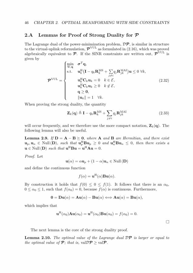
46 CHAPTER 2. OPTIMAL BEAMFORMING WITH SIDE CONSTRAINTS
2.A Lemmas for Proof of Strong Duality for PThe Lagrange dual of the power-minimization problem, DP , is similar in structureto the virtual-uplink reformulation, PVUL as formulated in (2.16), which was provedalgebraically equivalent to P . If the SINR constraints are written out, PVUL isgiven by
PVUL =
⎧⎪⎪⎪⎪⎪⎪⎪⎪⎪⎪⎨⎪⎪⎪⎪⎪⎪⎪⎪⎪⎪⎩
minU,q
σTq,
s.t. uHk
(I− qkRMS
k +∑j �=iqjRMAI
jk
)u ≤ 0 ∀k,
uHkCkuk = 0 k ∈ E ,
uHkCkuk ≥ 0 k ∈ E ,
q ≥ 0,‖uk‖ = 1 ∀k.
(2.32)
When proving the strong duality, the quantity
Zk(q) � I− qkRMSk +
∑j �=iqjRMAI
jk (2.33)
will occur frequently, and we therefore use the more compact notation, Zk(q). Thefollowing lemma will also be useful.
Lemma 2.9. If D = A −B � 0, where A and B are Hermitian, and there existup,un ∈ Null (D), such that uH
pBup ≥ 0 and uHnBun ≤ 0, then there exists a
u ∈ Null (D) such that uHBu = uHAu = 0.
Proof. Letu(α) = αup + (1− α)un ∈ Null (D)
and define the continuous function
f(α) = uH(α)Bu(α).
By construction it holds that f(0) ≤ 0 ≤ f(1). It follows that there is an α0,0 ≤ α0 ≤ 1, such that f(α0) = 0, because f(α) is continuous. Furthermore,
0 = Du(α) = Au(α)−Bu(α)⇐⇒ Au(α) = Bu(α),
which implies that
uH(α0)Au(α0) = uH(α0)Bu(α0) = f(α0) = 0.
The next lemma is the core of the strong duality proof.
Lemma 2.10. The optimal value of the Lagrange dual DP is larger or equal tothe optimal value of P; that is, valDP ≥ valP.

2.A. LEMMAS FOR PROOF OF STRONG DUALITY FOR P 47
Proof. The result is proved by showing that any optimal point of DP is in thefeasible set of PVUL. It follows that
valDP ≥ valPVUL = valP ,because DP and PVUL have the same criterion function.
Consider the Lagrange dual DP . The feasible set is given by all (μ1, . . . , μK ,q)that satisfy
Dk(q, μk) � 0 ∀k,qk ≥ 0 ∀k,μk ≥ 0 k ∈ E ,
whereDk(q, μk) � Zk(q)− μkCk,
and Zk(q) is defined in (2.33). The feasible set of PVUL on the other hand is givenby q satisfying
uHk Zk(q)uk ≤ 0 ∀k,
uHkCkuk = 0 k ∈ E ,
uHkCkuk ≥ 0 k ∈ E ,qk ≥ 0 ∀k,
for some uk, ‖uk‖ = 1. Note that for an optimal point q� of the Lagrange dual,DP , Dk(q�, μk) cannot be strictly positive definite for any feasible μk, because thatwould allow qk to be increased without violating any constraints, contradicting theoptimality of q�; that is,
Dk(q�, μk) � 0 ∀μk ∈ R (∀μk ≥ 0) for k ∈ E (k ∈ E). (2.34)
Next, consider the kth constraint of DP at a point (μ1, . . . , μK ,q�) that is optimalwith respect to the Lagrange dual, DP .
Case 1: k ∈ E , μk = 0 and μk cannot be increased without violating the con-straints.μk = 0 =⇒ Zk = Dk � 0. Assume uHCku < 0 ∀u ∈ Null (Zk). This impliesthat μk can be increased without violating the constraint on Dk, which is acontradiction. Hence there is a u = 0 such that uHZku = 0 and uHCku ≥ 0;that is, q� is in the feasible set of PVUL.
Case 2: k ∈ E or μk > 0To analyze this case, the following sets are defined:
Cp ={
u : uHCku ≥ 0, ‖u‖ = 1}, Cn =
{u : uHCku ≤ 0, ‖u‖ = 1
}.

48 CHAPTER 2. OPTIMAL BEAMFORMING WITH SIDE CONSTRAINTS
Both of these sets must be non-empty. If Cp = ∅ then (2.32) is infeasible, andthe optimal value of the Lagrange dual is infinity. If Cn = ∅, then Ck � 0and condition (2.34) is violated, because a small decrease of μk would makeDk(q�, μk) � 0.Next, we show that there exists un,up ∈ Null (Dk) such that un ∈ Cn andup ∈ Cp. It follows from Lemma 2.9 that there exists a u such that uHZku = 0and uHCku = 0 and the optimal point q� is thus in the feasible set of PVUL.Assume uHDku > 0 ∀u ∈ Cn. Hence uHDku = 0,u = 0, implies thatuHCku > 0 and condition (2.34) is violated, because a small decrease of μkwill make Dk � 0. Thus there exists a un such that un ∈ Null (Dk) andun ∈ Cn.Assume uHDku > 0 ∀u ∈ Cp. Hence uHDku = 0,u = 0, implies thatuHCku < 0. This violates condition (2.34), because a small increase of μkwill make Dk � 0. Thus there exists a up such that up ∈ Null (Dk) andup ∈ Cp.
2.B Proof of Strong Duality for GProof. The strong duality is proved by showing that there is an optimal point(ν�,u�) of the dual problem satisfying
ν�u�HCu� = 0 (2.35)u� ∈ PC (2.36)
which proves that u� is in the feasible set of the primal problem and that theprimal and dual criterion functions attain the same value at this point. It followsthat valG ≥ valDG, which combined with (2.29) proves the desired result.
Case 1: k ∈ E and ν� = 0This corresponds to the case that ν can be increased (but not decreased)from ν� without violating ν ∈ Vk. This implies that there exists a u� in theeigenspace associated with λmax such that u�HCu� ≥ 0, because otherwiseλmax(R + ν�C,Q) could be decreased by increasing ν�. (ν�,u�) therebysatisfies conditions (2.35) and (2.36).
Case 2: k ∈ E or ν� > 0This corresponds to the case that ν can be both increased and decreased fromν� without violating ν ∈ Vk. By the same argument as in case 1, there existsa up in the eigenspace associated with λmax, such that uH
pCup ≥ 0.Similarly there must exist a un in the eigenspace of λmax, such that uH
nCun ≤0, because otherwise λmax(R + ν�C,Q) could be decreased by decreasing ν.

2.C. PROOF OF THEOREM 2.8 49
Let u(α) = αup + (1− α)un and note that u(α) also is an eigenvector asso-ciated with λmax. Define the real continuous function f(α) = u(α)HCu(α).It holds that f(0) ≤ 0 ≤ f(1) and thus there exists an α0 ∈ [0, 1] such thatf(α0) = u(α0)HCu(α0) = 0. It follows that u� = u(α0) satisfies condi-tions (2.35) and (2.36).
2.C Proof of Theorem 2.8
Proof. The derivation of the gradient of Γ�(γ) � valΓ(γ) is based on the optimalityconditions of Γ . For notational convenience, we will not explicitly state the depen-dence on γ, and use Γ� in place of Γ�(γ). The optimal downlink and virtual-uplinkpowers, p� and q�, respectively, solves the eigenvalue problems (2.8) and (2.24),respectively, which are restated here for convenience,
Υpext = 1Γ�pext, pext = [p�, 1]T, (2.37)
Λqext = 1Γ�qext, qext = [q�, 1]T, (2.38)
where the matrices, Υ and Λ, are the extended downlink and virtual-uplink cou-pling matrices as defined in (2.9) and (2.25), respectively. The optimal powers areobtained from the first elements of the extended power vectors, pext and qext, bynormalizing them such that the last element is 1. Observe that it follows directlyfrom (2.37) that the left eigenvector of Λ is given by
ΛTpext = 1Γ� pext, where pext � Tpext, T �
[Ψ 00 Pmax
],
because ΛT may be factorized as ΛT = TΥT−1.Next, consider the derivative of Γ�(γ) with respect to γn. Define λ(γn) as the
eigenvalue of optimality condition (2.38), λ(γn) � 1/Γ�. The sought derivative maybe expressed in terms of the derivative of Λ,
Λ′ � ∂
∂γnΛ =
[I
σT
Pmax
]∂
∂λn
[DΨT D1
]=
[I
σT
Pmax
] [D′ΨT + D(Ψ′)T D′1
]︸ ︷︷ ︸�An
, (2.39)
as∂
∂γnΓ�(γ) = − λ
′(γn)λ2(γn)
= −Γ�2λ′(γn) = −Γ�2 pTextΛ′qext
qTextpext
,

50 CHAPTER 2. OPTIMAL BEAMFORMING WITH SIDE CONSTRAINTS
where the last identity follows from [HJ85, Theorem 6.3.12] because pext is a lefteigenvector of Λ. This holds whenever λ(γn) is a simple eigenvalue; that is, thesolution is unique. In the following, all beamformers and power allocations refer tothe optimal point, for a given γ, but for notational brevity they are not explicitlymarked (e.g., p�) as such. By expanding Λ′ as in (2.39), the above expression yields
∂
∂γnΓ�(γ) = −Γ�2 (Ψp + σ)TAnqext
qTΨp + Pmax= −Γ�pTD−1Anqext
qTΨp + Pmax, (2.40)
where the last identity is obtained by applying (2.10). The kth element of the vector,Anqext, is obtained straightforwardly by explicitly writing out the derivatives as
[Anqext]k = [D′(ΨTq + 1) + D(Ψ′)Tq]k
=(δkn − 2γk�
{uHkRdesk u′k
uHkRdesk uk
}) =qk/SINRVULk = qk
Γ�γk︷ ︸︸ ︷uHk
(qkRSI
k +∑j �=k qjRMAI
jk + I)uk
uHkRdesk uk
+
+ 2γk�{
uHk
(qkRSI
k +∑j �=k qjRMAI
jk
)u′k
uHkRdesk uk
}
= qkΓ�γkδkn +
2γk�{
uHk
(qkRSI
k +∑j �=k qjRMAI
jk − qkΓ�γkRdes
k
)u′k
}uHkRdesk uk
,
(2.41)
where δkn is the Kronecker delta function (i.e., δkn = 1 for k = n and zero other-wise). This expression may be further simplified by using Theorem 2.6 and Corol-lary 2.7, which state that the optimal beamformers, u�k, that solve (2.14), satisfythe generalized eigenvalue problem,
qkΓ�γk
(Rdesk + ν�kCk)uk = (qkRSI
k +∑j �=kqjRMAI
jk + I)uk,
where ν�k is the optimal dual point of (2.28). Rearranging terms and multiplyingthis with u′Hk yields
qkΓ�γkν�k�
{uHkCku′k
}= �
⎧⎨⎩uHk
(qkRSI
k +∑j �=kqjRMAI
jk −qk
Γ�γkRdesk
)u′k
⎫⎬⎭ , (2.42)
where the identity �{uHk Iu′k
}= �{uH
k u′k}
= 0, which follows from the normaliza-tion ‖uk‖ = 1, was used. Substitute (2.42) into (2.41) to obtain
[Anqext]k = qkΓ�γkδkn + qkΓ�
2ν�k�{
uHkCku′k
}uHkRdesk uk
= qkΓ�γkδkn, (2.43)

2.C. PROOF OF THEOREM 2.8 51
where the last identity follows from Corollary 2.7 by taking the derivative of theidentity ν�kuH
kCuk = 0 as
0 = ∂
∂γnν�kuH
kCuk = ν�k′uHkCkuk︸ ︷︷ ︸=0
+2ν�k�{
uHkCku′k
}= 2ν�k�
{uHkCku′k
}.
The claim that ν�k′uHkCkuk = 0 may be proved as follows. It obviously holds for
uHkCuk = 0, thus it can be assumed that uH
kCkuk > 0. By continuity in γn, itholds that uH
k (γn + ε)Ckuk(γn + ε) > 0 for sufficiently small |ε|. It follows thatν�k(γn + ε) = 0 for sufficiently small |ε| because ν�kuH
kCuk = 0 must be satisfied.Hence the derivative ν�k
′ is zero, which proves the claim.Theorem 2.8 follows by combining (2.40) and (2.43).


Chapter 3
Applications for ConstrainedBeamforming
In this chapter, we show how to use indefinite quadratic constraints for various ap-plications. In particular, we consider path-diversity constraints for CDMA systems,and show that these fall under the class of quadratic indefinite constraints. We showthat the diversity constraints significantly reduce the variance of the instantaneousSINR of the RAKE combined signal; that is, the probability of outage is decreased.Other applications of indefinite constraints include interference limitations in somespatial directions, or more general constraints on the total inter-cell interference.
3.1 Path Diversity in DS-CDMA
Consider a DS-CDMA system modeled in line with Section 1.5. DS-CDMA systemstypically use a high signaling rate (chip rate) and substantial multi-path propaga-tion is expected. By equipping the receiver with a RAKE combiner the contributionof each signal path is coherently combined at the receiver. This has many advan-tages, in particular:
• The combined signal power is increased without noise enhancement.
• The coherent combining increases the diversity.
If the received signal power is evenly distributed over several independently fadingsignal paths, a high diversity link that is robust to channel fading, is obtained. Byincreasing this path diversity the variance of the instantaneous SINR is decreased.This is desirable because a small variance of the SINR allows a relatively smallSINR margin for a given outage probability.
Assuming that the transmitter has only channel distribution information, it canevaluate only the long-term SINR, averaged over several channel realizations. Itcan thus not optimize the beamformers on a per channel realization basis, because
53

54 CHAPTER 3. APPLICATIONS FOR CONSTRAINED BEAMFORMING
the channel may vary too rapidly to be reliably estimated and fed back to thetransmitter. The beamformers are therefore optimized only with respect to theaverage SINR.
As derived in Appendix C.2, the long-term (average) SINR of the RAKE com-bined signal of user k, is well approximated (from below) by
SINRk = G wHkRdesk wk
wHkRIFIk wk +
∑j �=kwH
j RMAIk wj + σ2
k
, (3.1)
where G is the processing gain,
Rdesk �
∑τ∈LRAKE
k
E{
hk(τ)hHk (τ)
},
RMAIk �
Lh−1∑τ=0
E{
hk(τ)hHk (τ)
},
RIFIk � RMAI
k −∑
τ∈LRAKEk
βk(τ)E{
hk(τ)hHk (τ)
},
βk(τ) =E{‖hk(τ)‖2
}Tr
{Rdesk
} ,and LRAKE
k is the RAKE finger assignment of user k1. The self interference, of-ten referred to as the inter-finger interference (IFI) in CDMA contexts, is onlyapproximated by wH
kRIFIk wk. The reason for this approximation is that the exact
expression, given by (C.6), is not a quadratic form in wk. This is an immediate con-sequence of the (maximum ratio) combining weights that implicitly depend on thebeamformer. However, the approximation is pessimistic; that is, the approximationtypically overestimates the IFI.
When the beamformers are optimized with respect to the average SINR, theytend to direct the vast majority of the signal power along the signal path with theleast attenuation. This is of course beneficial from an average SINR perspective,but it decreases the path diversity and thereby the robustness of the link. Thequadratic indefinite constraints, presented herein, provide a framework to avoidthis problem and ensure diversity gain. Typically the most direct path, or the line-of-sight (LOS) path, dominates the power delay profile of the channel and a usefuldiversity constraint is thus to limit the fraction of the power that may be receivedalong the dominant path.
The average power received along the dominant or LOS component may bewritten as
PLOSk = E
{∥∥hHk (τLOSk )wk
∥∥2} = wHk E
{hk(τLOS
k )hHk (τLOSk )
}wk � wH
kRLOSk wk,
1We assume that the RAKE finger assignment is not updated for each channel realization,but is based on the long-term statistics of the channel.

3.1. PATH DIVERSITY IN DS-CDMA 55
where τLOSk is the delay of the signal arriving from the LOS path to the kth user.
The signal power received by the LOS path, may thus be limited to a maximumfraction β of the total received signal power using the constraint
wHkRLOSk wk ≤ βwH
kRdesk wk ⇐⇒ wH
k
(βRdesk −RLOS
k
)wk ≥ 0,
which is a quadratic indefinite constraint of the desired form (2.2), where
Ck = βRdesk −RLOS
k .
The cost of increasing the diversity using diversity constraints is that the trans-mission power required to meet a desired average SINR target is increased. There-fore there is a trade off between average SINR and diversity; this trade off is inves-tigated next.
Simulation scenarioThe effects of diversity constraints are demonstrated by simulating a single cellscenario, illustrated in Figure 3.1a, with three co-channel users. The users have thesame distance to the base station: Their mutual distances are also equal. The basestation is equipped with a uniform circular array (UCA) with N = 10 antennas.The distance between the antennas is set to the wavelength of the carrier.
The multi-path channel is modeled as a tapped delay line with Lh = 10 taps,each modeled as independently Rayleigh fading. Each tap is assigned a correspond-ing scattering cluster, illustrated by the circles in Figure 3.1a. We also assume thatthere is local scattering in the close proximity of each user. This is simulated as ascattering cluster centered around each user, which motivates the Rayleigh fadingchannel model. The scatterers are assumed to be Gaussian distributed within eachcluster with an angular spread of 2 degrees; that is, the standard deviation of thescatterers’ positions is 2 degrees [ZO94b]. The correlation matrices are computedusing the approximate expressions given in [VBO04].
The correlation matrices, assumed known at the transmitter, are scaled accord-ing to an exponentially decaying power delay profile, except for the first tap, whichis twice as strong as suggested by an exponential profile, see Figure 3.1b. Such,worst case, scenarios are particularly penalized by the beamformer optimization,which will direct the vast majority of the power along the dominant tap. The RAKEreceivers were simulated using LRAKE = 5 fingers, combining the signal power fromthe first channel taps—that is,
LRAKEk = {0, 1, . . . ,LRAKE − 1}
—of which the zeroth corresponds to the LOS component.We solved the downlink beamforming problem with diversity constraints for
different values of β in the diversity constraint. To ensure a fair comparison, wekept the total transmission power fixed and solved Γ to maximize the long-term

56 CHAPTER 3. APPLICATIONS FOR CONSTRAINED BEAMFORMING
(a) Simulation scenario
0 1 2 3 4 5 6 7 8 90
0.1
0.2
0.3
0.4
0.5
0.6
Channel Tap, τ
P(τ
)
(b) Power delay profile, P (τ) = E{‖hk(τ)‖2
}Figure 3.1: Illustration of the CDMA system. The three co-channel users aredistributed uniformly around the base station. The presented simulation resultbelong to the bottom left user, but all three users have similar performance. Thescattering clusters are marked with circles in (a). In the power delay profile (b),the LOS component is chosen stronger than the exponential profile.
SINRs of the users. The transmission power was set such that every user achieves,
SINRk = γk = γ = 10 dB ∀k,
without any diversity constraint (i.e., for β = 1). If β is increased, the long-termSINR decreases, because the optimization then become more constrained.
3.2. INTERFERENCE CONSTRAINTS 57
Simulation resultsThe distribution of the received power over the RAKE fingers and the cumulativedistribution function (CDF) of the instantaneous SINR were computed for differentβ by means of Monte Carlo simulations. The instantaneous SINR of the RAKEcombined signal is given by (C.3) in Appendix C.
Figure 3.2a shows how the total received signal power is distributed over theRAKE fingers for different β. It is interesting to note that without any diversityconstraint (β = 100%) more than 90% of the received power is contributed by thefirst RAKE finger, which is substantially more than what isotropic (single antenna)transmission results in (i.e., more than the power profile of the channel taps sug-gests). This is because the beamformer tends to focus most of the transmittedpower along the path with least average attenuation. As β is decreased, it is appar-ent from Figure 3.2a that the received power becomes more evenly distributed overthe RAKE fingers. As β is decreased the path diversity of the link increases, whichis shown by the increased slope of the CDF of the instantaneous SINR, plotted inFigure 3.2b. Increasing the slope of the CDF decreases the probability for poorSINR realizations.
As shown in Figure 3.2b it is possible to substantially decrease the probabilityof deep fades in the SINR by using diversity constraints. However, as β is decreasedthe average SINR is also decreased due to the fixed transmission power. Thereforethere is a trade off between the average SINR and the variance. Optimizing β interms of outage, or any criterion, is however quite involved, because it typicallydepends on the current scenario and several system parameters. Moderate valuesof β ≈ 0.8 do however give a good protection against worst case scenarios, such asthe one considered in the simulations.
3.2 Interference Constraints
In any multiuser cellular system co-channel interference is typically a limiting factor.The co-channel interference within a cell is efficiently suppressed in the downlinkbeamforming optimization by utilizing the CSI or CDI at the base station. Howeverthe performance of co-channel users that are not included in the optimization (e.g.,users assigned to neighboring cells) can be severely penalized. Depending on theamount of channel knowledge available at the base station of these interfered users,the interference to the inter-cell users can be limited, or for instance the totalpower radiated in a sector can be limited, by applying indefinite constraints in theoptimization problem. Other scenarios where interference limiting is useful includewarfare scenarios, where radiation in some directions (e.g., directions of sensors)are unwanted.
Techniques for limiting interference have previously been based on so-callednulling, where all the beamformers are forced to have nulls placed to the interfereduser(s); that is, the beamformers are confined to the subspace orthogonal to theseusers. This is however an unnecessarily strict requirement, because interference is

58 CHAPTER 3. APPLICATIONS FOR CONSTRAINED BEAMFORMING
0 1 2 3 40
0.2
0.4
0.6
0.8
1
RAKE finger
β = 1 (No constraint)
β = 0.8
β = 0.6
(a) Relative Distribution of Received Power
0 5 10 15
0.1
0.05
0.02
1
0.5
[dB]
SINR (dB)
β = 1 (No constraint)
β = 0.8
β = 0.6
(b) Cumulative Distribution Function of the SINR
Figure 3.2: Results of path-diversity simulation. Without diversity constraintsmore than 90% of the signal power is received from the first tap (a), resulting insubstantial variance of the instantaneous SINR. As β is decreased the diversityincreases, which is shown by the steeper slopes of the CDF (b). However, as thediversity increases, the average SINR decreases. The probability of particularly lowSINR realizations decreases notably for smaller values of β.
pushed below the noise level. The framework of indefinite constraints allows forless strict constraints, with nulling as a special case.
For simplicity, consider a single cell of a narrowband system. Let hk be thechannel vector of user k. The received signal may thus be modeled as (1.7); that

3.2. INTERFERENCE CONSTRAINTS 59
is,
rk(t) =K∑j=1
hHkwjsj(t) + nk(t),
where K is the number of users assigned to the cell.
Relaxed nullingConsider now a user of a different cell, which therefore is not included in the SINRoptimization, but for which we still want to limit the interference. Let h0 be thechannel vector from the base station to this user. The interfering power from userk to this user is given by
Ik =∥∥hH
0 wk∥∥2 = wH
k h0hH0 wk. (3.2)
A useful interference constraint is to limit the interference caused by user k to afraction β of the worst case interference,
Ik ≤ βImaxk = β ‖h0‖2 ‖wk‖2 , (3.3)
where the worst case interference, Imaxk , is obtained when wk is parallel with h0.
Note that classical nulling is obtained as the special case β = 0. By combining(3.2) and (3.3) the interference constraint may be written as
wHk
(βI− h0hH
0
‖h0‖2)
wk ≥ 0, (3.4)
which is a quadratic indefinite constraint of the desired form (2.2), with Ck =βI− h0hH
0 / ‖h0‖2.To demonstrate the benefits of relaxed nulling, a cell of a communication system
was simulated. The base station was simulated using a UCA with 3 antenna ele-ments that are separated by 0.5 wavelengths. In each scenario, users were randomlypositioned, from a uniform distribution, within the circular cell. The position of theinterfered user was also randomly generated, in each scenario. The channel realiza-tion of each user, known at the base station, was drawn from a correlated Rayleighfading distribution, with a correlation matrix generated for a cluster of Gaussiandistributed scatterers, centered at the user position, with an angular spread of 2degrees [ZO94b]. At the cell border, the average SNR of each antenna was set to,
PmaxE{|[h]n|2
}σ2k
= 10γ ∀n,
where γ is the target SINR of each user and [h]n denotes the nth element of thechannel vector h. For users within the cell the channel covariance matrix was scaledproportional to r−2, where r is the distance to the base station.

60 CHAPTER 3. APPLICATIONS FOR CONSTRAINED BEAMFORMING
0 5 100
1
2
3
4
[dB]γ
Ass
igne
dus
ers
β = 1 β = 0.1 β = 0.02 β = 0
Figure 3.3: The average number of users that could be simultaneously assigned inthe cell without violating the SINR constraints, for different interference constraintsand SINR targets.
The optimization problem, Γ , was solved for different interference constraints,and new randomly positioned users were assigned until the SINR targets could notbe met—that is, until the minimum normalized SINR, SINRmin ≤ 1. The averagenumber of users that could simultaneously meet the SINR targets, for the differentinterference constraints, were evaluated using Monte Carlo simulations. The sim-ulation results are shown in Figure 3.3. It is clear how relaxing the interferenceconstraints significantly improves performance, in particular for low SINR. Notethat for γ = 0dB, the relatively strict interference constraint with β = 2%, stillresults in a performance increase of 27% over classical nulling.
Limiting the power radiated in a sectorIn scenarios where it is not reasonable to assume that the channel h0 of the inter-fered user is known at the base station, it may still be reasonable to assume that theposition is known to be in some sector, based on for instance the frequency plan-ning of the cells. A reasonable interference constraint for such a scenario is to limitthe power transmitted within this sector to a fraction β of the total transmissionpower.
The power transmitted in the sector [θ0 −Δθ, θ0 + Δθ] by user k is given by
Pθ0k = wH
k
(1
2π
∫ Δθ
−Δθa(θ0 + φ)aH(θ0 + φ)dφ
)wk � wH
kRθ0wk,
where a(θ) is the array response of the base station for a plane wave arriving fromangle θ. The interference constraint is thus given by
Pθ0k ≤ β ‖wk‖2 ⇐⇒ wH
k (βI−Rθ0) wk ≥ 0.

3.2. INTERFERENCE CONSTRAINTS 61
Note that Rθ0 is typically of full rank. Choosing β = 0 will therefore result in aninfeasible scenario. Limiting the interference within a sector in this way is thusnot possible using traditional nulling. Techniques for limiting the interference ina sector using nulling typically places nulls on several sample points in the sector.However, such schemes do penalize the performance severely, because each nullreduces the dimension of the subspace in which the beamformers are confined.
Suppression of inter-cell interferenceIn a decentralized system, where each base station chooses the beamformers withoutcoordination with other base stations, inter-cell interference is a significant limitingfactor.
However, by listening to the uplink streams, it is possible for a base stationto estimate the statistical behavior of the inter-cell interference. Let R0 be thesecond order statistics of the inter-cell interference. The expected total interferingpower (from user k) received by the neighboring cell users may thus be limited toa fraction β of the worst case interference:
wHkR0wk ≤ βλmax ‖wk‖2 ,
where λmax is the largest eigenvalue of R0.

Chapter 4
User Selection with MMSE SINREstimation
Downlink resource allocation in multiuser communication systems with multipletransmit antennas is a nontrivial task. In this chapter—and the remainder of thisthesis—we consider a best-effort system with elastic data traffic. In each time (andfrequency) slot, the resource scheduler determines the users that may access thechannel, and assigns a beamformer to each selected user. The long-term designgoal of the recourse allocation is to maximize the system performance in terms ofthroughput and reliability without compromising performance fairness among theusers.
The user selection is an essential part of downlink SDMA. If the allocated usersare spatially compatible, the transmitter (base station) can form non-interferingsignal beams, without signal degradation. The user-selection algorithm, shouldalso utilize multiuser diversity: The selected users should, not only be spatiallycompatible, but also have a high channel gain. To identify these characteristics,the transmitter must have instantaneous CSI, which can only be estimated at thereceiver: We are assuming an FDD system. In multiuser systems the feedbackcapacity is shared, and generally only a limited feedback rate is alloted each user;that is, only partial CSI can be made available at the transmitter.
In this chapter, an MMSE SINR estimation framework is proposed where limitedinstantaneous CSI feedback (partial CSI) is combined with statistical information.This framework is applied in an SDMA setting, and several downlink SDMA re-source allocation algorithms, of varying computational complexity, are proposed toutilize the MMSE estimates. The throughput vs. fairness trade-off is balanced byconsidering a weighted sum-rate criterion function in the scheduling; for example,proportional fair scheduling [KMT97, VTL02] can be implemented.
63

64 CHAPTER 4. USER SELECTION WITH MMSE SINR ESTIMATION
4.1 System Assumptions
The downlink of a single cell system is considered, where the base station is equippedwith nT transmit antennas. The receivers each have a single receive antenna andthe narrowband channel of user k ∈ {1, . . . ,K} is modeled by the channel vectorhk ∈ CnT . The channel is modeled as a stochastic vector variable that is realizedonce in each block in which it remains static; that is, the channel is modeled asblock fading. We assume that the kth receiver can perfectly estimate any requiredproperties of hk (i.e., the feedback parameters). The transmitter knows only thedistribution of hk, and the partial CSI conveyed by feedback parameters. Weassume a flat-fading channel: The symbol sampled, complex base band equivalentof the received narrowband signal is modeled as
rk(t) = hHk x(t) + nk(t), (4.1)
where nk(t) is AWGN with power σ2k and x(t) ∈ CnT is the vector of transmit-
ted signals. Even though a narrowband channel assumption is thus made, butthe theory generalizes straightforwardly to wideband OFDM systems, where eachsubcarrier can be treated as a separate narrowband channel, see Section 1.5.
A wide-area, or metropolitan-area, scenario is considered with the channel vectordistributed as
hk ∈ CN (hk,Rk),
where the covariance matrix, Rk, is assumed to be dominated by a single (or a few)eigenmodes (i.e., there is significant correlation), which is typical for cellular systemswith elevated base stations [ECS+98]. Note that the statistical information of thechannel, hk and Rk, change on a much longer time scale than the small-scale fadingof the channel. It is therefore assumed that the transmitter is able to perfectlytrack the moments of the channel. Note that the downlink channel statistics canbe estimated directly at the base station from the reverse communication link, evenif the downlink and uplink channels are separated in frequency [CHC04].
Let S be the set of users that are scheduled for transmission in the current timeslot. In an SDMA system, S typically contains more than one user. In systemsrelying only on CDI and CGI (channel norm) feedback, single stream beamform-ing is optimal with respect to ergodic capacity, for sufficiently large realizations ofthe CGI parameter [JHO07]. With many users in the system, the CGI parame-ters likely belong to this beamforming optimality range. Therefore, we consider abeamforming system where the signal, xk(t), intended for user k, is mapped ontothe antenna array with the beamforming vector, wk,
x(t) =∑k∈S
wkxk(t). (4.2)
In line with Section 1.4, the instantaneous SINR of user k ∈ S for a given channel
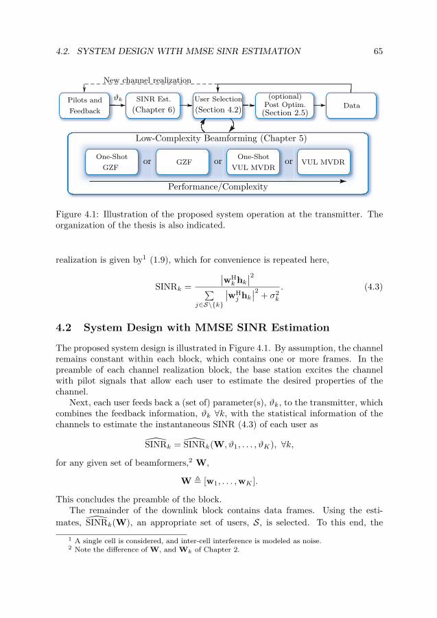
4.2. SYSTEM DESIGN WITH MMSE SINR ESTIMATION 65
Pilots andFeedback
SINR Est.(Chapter 6)
User Selection(Section 4.2)
(optional)Post Optim.
(Section 2.5)Data
New channel realization
ϑk
Low-Complexity Beamforming (Chapter 5)
One-ShotVUL MVDR
VUL MVDROne-Shot
GZFGZF
Performance/Complexity
ororor
Figure 4.1: Illustration of the proposed system operation at the transmitter. Theorganization of the thesis is also indicated.
realization is given by1 (1.9), which for convenience is repeated here,
SINRk =∣∣wHk hk
∣∣2∑j∈S\{k}
∣∣wHj hk
∣∣2 + σ2k
. (4.3)
4.2 System Design with MMSE SINR Estimation
The proposed system design is illustrated in Figure 4.1. By assumption, the channelremains constant within each block, which contains one or more frames. In thepreamble of each channel realization block, the base station excites the channelwith pilot signals that allow each user to estimate the desired properties of thechannel.
Next, each user feeds back a (set of) parameter(s), ϑk, to the transmitter, whichcombines the feedback information, ϑk ∀k, with the statistical information of thechannels to estimate the instantaneous SINR (4.3) of each user as
SINRk = SINRk(W, ϑ1, . . . , ϑK), ∀k,for any given set of beamformers,2 W,
W � [w1, . . . ,wK ].
This concludes the preamble of the block.The remainder of the downlink block contains data frames. Using the esti-
mates, SINRk(W), an appropriate set of users, S, is selected. To this end, the1 A single cell is considered, and inter-cell interference is modeled as noise.2 Note the difference of W, and Wk of Chapter 2.

66 CHAPTER 4. USER SELECTION WITH MMSE SINR ESTIMATION
user-selection algorithm calls a low-complexity beamforming function for each can-didate user group. As an optional post-optimization step the beamformers of theselected users can be optimized using a more computationally demanding beam-forming criterion. Next, data is transmitted to the scheduled users. In consecutiveframes, new sets of users may be selected to achieve better fairness. Note thatthe beamformers, wk, k ∈ S, are not assumed known to the scheduled receivers.Thus, the effective scalar channel, hH
kwk, must be estimated at user k during thedata transmission interval in order to perform coherent detection. This could forinstance be done by initializing the data transmission to each user with a short,dedicated pilot signal.
Instantaneous channel and SINR estimation
The feedback parameters, ϑk, provide information about the instantaneous channelsand are combined with the CDI (channel moments) known a priori to the trans-mitter. Using an MMSE framework the transmitter estimates the instantaneousmoments of the channels as
hk �E {hk | ϑk} , Qk �E{
hkhHk
∣∣ ϑk} , (4.4)
where channel realizations of different users are assumed independent. Using theconditional correlation matrix, Qk, the MMSE estimate of the signal/interferencepower,
∣∣hHkwi
∣∣2, for a given ϑk, is obtained as
E{∣∣hH
kwi∣∣2 ∣∣ϑk} = wH
i Qkwi.
The instantaneous SINR in (4.3) can thus be estimated as3
SINRk = wHk Qkwk∑
i∈S\{k}wHi Qkwi + σ2
k
. (4.5)
The conditional moments, hk and Qk, are however in many cases non-trivial tocompute. In Chapter 6, we show how to efficiently compute these quantities whenthe feedback parameter is ρk = ‖hk‖2. The framework is extended in Chapter 8where we consider the more general feedback parameter, ζk = ‖Akhk‖2, where Akis an arbitrary matrix of choice.
3Note that the estimate is not the MMSE estimate of the instantaneous SINR; that is, wedo not estimate the instantaneous SINR as E{SINRk | ρ1, . . . , ρK}. However, the estimate isthe SINR of the conditional channel (i.e., the expected signal power over the expected noise andinterference power ratio), even though it is non ergodic (unless we code over multiple conditionalchannel realizations).

4.2. SYSTEM DESIGN WITH MMSE SINR ESTIMATION 67
Optimal user selection and beamformingAllocating system resources to the users is a balance between total system through-put and fairness among the users. Also, the multiuser diversity should be exploitedto increase the throughput while ensuring that the delays are kept at a reasonablelevel.
To take all these factors into account the design of the joint scheduling, powercontrol, and beamforming is based on a weighted sum-rate criterion
RΣ(W) =∑k∈Sβk R
(SINRk(W)
), (4.6)
where R(SINR) is the rate function (assumed non-decreasing) that maps an SINRto transmission rate. The weights, βk, determine the priority of users and can bechosen according to, for instance, the proportional fair scheduling criterion [KMT97,VTL02]. Optimally the beamformers and power allocation should be chosen so asto maximize the weighted sum rate,
W� = arg maxW∈W
RΣ(W), (4.7)
whereW is the set of feasible beamformers and power allocations satisfying pi ≥ 0,and the sum-power constraint, 1Tp ≤ Pmax. The optimal set of scheduled users isimplicitly determined as S� = {k |p�k > 0}.
This optimization problem was analyzed in Section 2.5, where a more structuredform of the optimization problem was derived. The problem does however remainnon-trivial when all users are included in the optimization, and is therefore proposedas a post optimization step, see Figure 4.1, to the low-complexity greedy user-selection scheme proposed next.
Resource allocation with greedy user selectionAs mentioned above, optimally choosing a set of spatially compatible users, S,to schedule is a non-trivial problem. Instead a suboptimal greedy user-selectionscheme, similar to the approach in [DS05], is adopted and extended to an arbitrarybeamforming function. The proposed greedy user selection can be combined withany of the beamforming techniques discussed in the sequel. For now, the arbitrarybeamforming function is denoted as
WS = BF(S),
and determines the beamformers for the set of scheduled users, S, using some crite-rion. The complexity of the algorithms is significantly reduced if the beamformerscan be readily updated for a user set that is appended by a single user k. Toemphasize this we define the beamforming function
(WS∪{k},PS∪{k}) = BFAPPEND(k,S,PS),

68 CHAPTER 4. USER SELECTION WITH MMSE SINR ESTIMATION
1: C ← set of all users2: Wnew ← [ ], Snew ← ∅, RΣnew ← 0, PSnew ← ∅3: repeat4: W←Wnew, S ← Snew, RΣ ← RΣnew, PS ← PSnew5: for all k ∈ C do6: Sc ← S ∪ {k}7: (Wc,PSc )← BFAPPEND(k,S,PS)8: RΣ[k]← RΣ(Wc,Sc)9: if RΣ[k] > RΣnew then
10: RΣnew ← RΣ[k], Snew ← Sc, Wnew ←Wc, PSnew ← PSc11: end if12: end for13: C ←
{k∣∣k ∈ C, RΣ[k] > RΣ
}\ Snew
14: until S = Snew15: return S, W
Table 4.1: Outline of the resource allocation algorithm with greedy user selection
which computes the beamformers for the user set S ∪ {k} by using parameters inthe set PS , which were previously computed when considering the user set S. InSections 5.1 – 5.3, several low-complexity algorithms are proposed that can be usedin the beamforming allocation.
The proposed greedy resource allocation algorithm is given in Table 4.1. Insummary, each iteration of the algorithm is composed of three stages.
1. Line 6 – 8: Try adding each user in the set of candidates, C, to the set ofscheduled users, S, and evaluate the resulting weighted sum rate for eachcandidate.
2. Line 9 – 11: If the most favorable candidate increases the total weighted sumrate, add it to the set of scheduled users, S.
3. Line 13: Remove incompatible users from the set of candidates, C.These three steps are repeated until no more users are selected—that is, until
S = Snew.
Adapting for estimation errors
It is important to note that SINRk in (4.5) is an estimate of the actual instanta-neous SINR, and thus includes estimation errors. Overestimating the SINR is notdesirable because the channel does not support the allocated rate, resulting in anunacceptable packet/frame error rate. Overestimating the instantaneous SINR isreferred to as an outage. The outage probability can be remedied by coding overseveral transmission blocks that experience independent channel realizations—forexample, coding over several well separated sub-carriers in an ODFM system. To

4.2. SYSTEM DESIGN WITH MMSE SINR ESTIMATION 69
further reduce the outage probability to an acceptable level, the SINR can be pes-simisticly estimated to allow an estimation error margin. This could be a fixedback off, as in [HBO05b, HO06a], where a margin of 1.5-2 dB resulted in an outageprobability below 5%.
Having a non-adaptive back off margin does however have the disadvantage thatthe outage probability can vary greatly for different realizations of the feedbackparameters, ϑk, and the margin is therefore set unnecessarily high for most of therealizations. For example, with ϑk = {‖hk‖2} it was shown in the asymptoticanalysis in Section 6.4 that the relative estimation error will tend to zero as ‖hk‖2tends to infinity. This motivates an adaptive back off margin, based on the actualaccuracy of the estimate. The mean squared error (MSE) of the signal/interferencegain estimate, wH
i Qk(ϑk)wi, is obtained as
MSE(∣∣hHkwi
∣∣2 ∣∣ϑk) � E{[ ∣∣hH
kwi∣∣2 −wH
i Qk(ϑk)wi]2|ϑk
}(4.8)
= E{∣∣hH
kwi∣∣4 |ϑk}− (wH
i Qkwi)2, (4.9)
where MSE(x∣∣y), denotes the MSE of the estimate E {x|y}. The MSE is thus
readily obtained from the fourth order moment,
E{∣∣wH
i hk∣∣4 |ϑk} ,
which in turn is computed from the conditional PDF, f(hk|ϑk). How to efficientlycompute the fourth order moment does however depend on the choice of feedbackparameters. In Chapter 6 and Chapter 8 these moments are derived for the feedbackparameters ρk = ‖hk‖2 and ζk = ‖Akhk‖2, respectively. The MSE can be used toinclude an adaptive back off margin in the SINR estimate as
SINRMSEk =
max{
0,wHk Qkwk − α RMSE
(|wHk hk|2
∣∣∣ϑk)}∑i∈S\{k}
[wHi Qkwi + α RMSE
(|wHi hk|2
∣∣∣ϑk) ] + σ2k
, (4.10)
where RMSE (x|y) �√
MSE (x|y), is the root mean squared error (RMSE) and αis a tuning parameter, which is chosen to achieve a target frame error rate.
Computing SINRMSEk is more computationally demanding than computing
SINRk. Moreover, the form of (4.10) is typically unsuitable for beamformer op-timization. Therefore, the beamformer computations in BFAPPEND are performedwith respect to SINRk. The adaptive back off should however be included in therate adaptation and the user selection. The weighted sum-rate evaluation on Line8 of Table 4.1 is therefore computed with respect to SINRMSE
k .


Chapter 5
Low-Complexity Beamforming
The greedy user-selection algorithm, proposed in Chapter 4, relies on low-complexity beamforming algorithms. In this chapter, we develop several subopti-mal beamforming algorithms, with low complexity, that are suitable for the MMSESINR estimation framework. A generalized zero-forcing (GZF) algorithm, withlow complexity, is proposed. The GZF algorithm is more suitable for partial CSIthan traditional zero forcing (ZF) [God97b]. We also propose a beamforming al-gorithm using virtual-uplink duality and the minimum variance distortionless re-sponse (MVDR) criterion. This VUL MVDR beamforming achieves near optimalperformance at only a moderate complexity increase over GZF. The relative com-plexity and performance of the proposed beamforming algorithms, and their use inuser selection, is illustrated in Figure 4.1.
5.1 Generalized Zero Forcing
The design goal for the GZF algorithm is to maintain the low computational com-plexity of traditional ZF, but adapt it to better suit the CSI provided by the MMSESINR estimation framework. Before introducing GZF, we briefly summarize tradi-tional ZF.
Traditional zero forcingIf the channel vectors of all scheduled users are fully known at the transmitter, theintra-cell interference caused at user k is known to the transmitter and given by
Ik =∑
j∈S\{k}wHj
(hkhH
k
)wj , (5.1)
where S is the set of scheduled users. The ZF beamforming design criterion is torequire zero intra-cell interference:
For ∀k ∈ S find wk subject to Im = 0, ∀m ∈ S.
71

72 CHAPTER 5. LOW-COMPLEXITY BEAMFORMING
This criterion can be recast into a linear system of equations [God97b],
wHk hj = δjk, ∀j ∈ S,
and wk is obtained by normalizing wk according to the allocated transmissionpower. It is essential for this system of equations not to be over determined, whichposes the constraint |S| ≤ nT . The system of equations can also be written inmatrix form as
I = WHSHS , where
{HS �
[hS(1)hS(2) · · ·hS(|S|)
],
WS �[wS(1)wS(2) · · · wS(|S|)
],
and the elements of S are ordered as S(1), . . . ,S(|S|). The optimal solution to thissystem of equations is given by the Moore-Penrose pseudo inverse of HH
S ,
WS = HH†S = HS(HH
SHS)−1, (5.2)
which maximizes the received signal power at each user, subject to the constraintof zero intra-cell interference.
In a system with perfect CSI, zero-forcing beamforming performs well, in par-ticular when combined with user selection [YG06]—that is, when S is a set ofspatially compatible users. However, if the transmitter does not have perfect CSI,the orthogonality is lost due to estimation errors of hk, and co-channel interfer-ence is introduced in an uncontrolled manner. In such scenarios it is preferable,from an estimation error point of view, to use the MMSE estimator, wH
i Qkwi, toestimate the received signal/interference power, in favor of using a channel vectorestimate, hk, as |hH
kwi|2. This becomes particularly apparent when wi is chosenorthogonal to hk (as in ZF) because any such direction is rated as equally good andoptimistically estimated to yield zero interference by the criterion |hH
kwi|2. TheMMSE estimator, wH
i Qkwi, does however track the expected interference in anydirection, which makes it possible to avoid directions, in addition to hk, in whichit is likely to cause significant interference. Next, the ZF beamforming criterion ismodified to better take advantage of the information in Qk.
Generalized zero forcingUsing the MMSE estimation framework, the co-channel interference at user k isestimated at the base station as
Ik =∑j �=k
wHj Qkwj .
The design criterion of zero intra-cell interference, is too strict and cannot be ap-plied, because Qk is generally of full rank. Instead, an interference sensitive sub-space is identified for each user, where the interference is known to significantly

5.1. GENERALIZED ZERO FORCING 73
degrade the performance. This subspace is identified from the spectral (eigenvalue)decomposition of Qk as
Qk =[vk V(S)
k V(I)k
]Λk
[vk V(S)
k V(I)k
]H, (5.3)
where the eigenvalues are ordered decreasingly along the diagonal of Λk. Hence,vk is the dominating eigenmode of Qk, which is the beamforming direction that is(or rather expected to be) most favorable for user k. Thus vk takes the role of thechannel vector hk in classical zero forcing. Similarly,
V(I)k ∈ CnT×n
(I)k
spans the subspace associated with the n(I)k smallest eigenvalues, that is, the space
in which the user is insensitive to interference. The intermediate,
n(S)k = nT − n(I)
k − 1,
eigenmodes are represented by
V(S)k ∈ CnT×n
(S)k ,
which spans the space in which the user remains sensitive to interference. Similarto traditional zero-forcing design, the criterion of the proposed GZF algorithm,is to require the beamformer of each user to be orthogonal to vk of the otherscheduled users. In addition, the beamformer, wk, is required to be orthogonal tothe interference sensitive subspaces of all other scheduled users; that is,
∀k ∈ S : wk ∈ V(R)S\{k}, (5.4)
whereV(R)S �
{w
∣∣∣ wH[vj V(S)j
]= 0, ∀j ∈ S
},
is the aggregate restricted subspace associated with the users in S. Let the columnsof the matrix, V(R)
S , form an orthonormal basis of V(R)S —that is,
V(R)S = range
{V(R)S
}—then the interference constraint (5.4) can equivalently be formulated as
∀k ∈ S : wHkV(R)S\{k} = 0. (5.5)
The beamformer that maximizes the received signal power along vk, while satisfying(5.5), is similar to (5.2) obtained from the first column of the Moore-Penrose pseudoinverse,
[wkWdummy] = [vkV(R)S\{k}]
H†.

74 CHAPTER 5. LOW-COMPLEXITY BEAMFORMING
By taking advantage of VS\{k} being orthonormal, wk (differently scaled) is readilyobtained as
wk =(I−V(R)
S\{k}(V(R)S\{k})
H)vk � Π(A)S\{k}vk, (5.6)
where Π(A)S\{k} is the projection matrix onto the aggregate allowed subspace (i.e.,
the complement to the aggregate restricted subspace). The beamformer, wk, isfinally obtained by rescaling wk according to the transmit power allocation. In thisthesis, the GZF algorithm distributes the power equally among the scheduled users,but other choices [BPN06] can also be implemented.
A question that arises is how to choose the dimension of the interference insen-sitive subspace of user k, n(I)
k . This dimension balances the trade-off:
1. The larger n(I)k —the less constrained the other scheduled users become (i.e.,
the performance of the co-channel users increases and potentially more userscan be scheduled simultaneously).
2. The larger n(I)k —the larger interference at user k (i.e., the performance of
user k, when scheduled, decreases).
Herein, we let n(I)k = n(I) be a fixed system design parameter, but more elaborate
adaptive methods that take user and/or channel realization specific factors intoaccount can be considered.
The computational complexity of GZF arises from computing
Π(A)S\{k} � I−V(R)
S\{k}(V(R)S\{k}
)H ∀k.
In general, V(R)S is computed by applying the Gram-Schmidt orthogonalization
procedure to the columns of[vS(1)V
(S)S(1) . . .vS(|S|)V
(S)S(|S|)
].
However, in the user selection algorithms, a computational complexity reductioncan be achieved by sequentially adding users to the set of scheduled users, and up-date the projection matrices, Π(A)
S\{k}, in each iteration. This procedure is outlinedin Table 5.1a. In each iteration the function,
(W,PS∪{k}) = GZFAPPEND(k,S,PS),
is called, which updates the GZF beamformers to the user set, S ∪ {k}, by us-ing projection matrices previously computed for S. These projection matrices arecollected in the parameter set, PS ,
PS � {Π(A)S } ∪ {Π(A)
S\{k}| ∀k ∈ S}.

5.1. GENERALIZED ZERO FORCING 75
1: Sc ← ∅, P ← {Π(A)Sc = I}
2: for all k ∈ S do3: (W,P)← GZFAPPEND(k,Sc,P)4: Sc ← Sc ∪ {k}5: end for6: return wk, ∀k ∈ S
(a) Sequential implementation of GZF
1: input k, S, PS = {Π(A)S } ∪ {Π(A)
S\{kc}|∀kc ∈ S}2: set Π(A)
k ← Π(A)S and Π(A)
kc← Π(A)
S\{kc}, ∀kc ∈ S3: Sc ← S ∪ {k}4: for all kc ∈ Sc do5: V← Π(A)
kc[vkV(S)
k ]6: V(o) ← Orthonormalize V using Gram-Schmidt7: Π(A)
kc← Π(A)
kc− V(o)(V(o))H
8: end for9: Π(A)
Sc ← Π(A)k , Π(A)
k ← Π(A)S
10: ukc ←Π(A)kc
vkc∥∥Π(A)kc
vkc∥∥ , Π(A)
Sc\{kc} ← Π(A)kc, ∀kc ∈ Sc
11: return ukc , ∀kc ∈ Sc and PSc = {Π(A)Sc } ∪ {Π
(A)Sc\{kc}|∀kc ∈ Sc}
(b) Implementation of GZFAPPEND
Table 5.1: Outline of the GZF algorithm
In each iteration, GZFAPPEND(k,S,PS) computes the projection matrix, Π(A)S∪{k},
which projects onto the aggregated allowed signaling space that all subsequent can-didates are constrained to. This procedure is efficient because the allowed space—orrather its spanning basis vectors—are computed only once and reused for all sub-sequent users. The GZFAPPEND algorithm in Table 5.1b can be summarized asfollows:
1. Line 2-3: Define the set Sc � S ∪{k}, and initialize the matrices, Π(A)kc∀kc ∈
Sc, to the projection matrices in PS .
2. Lines 4–8: Update each projection matrix Π(A)kc
such that the range is or-thogonal to [vkV(S)
k ]. The updated matrices satisfy
Π(A)k = Π(A)
Sc and Π(A)kc
= Π(A)Sc\{kc} ∀kc ∈ S.

76 CHAPTER 5. LOW-COMPLEXITY BEAMFORMING
3. Line 10: Compute the GZF beamformers of the users.
The GZF algorithm is well suited for the greedy user-selection scheme proposedin Chapter 4, because the beamformers are readily updated when a single user isappended to S. GZF matched with the greedy user selection proposed in Chapter 4,has many similarities with the greedy user selection with traditional ZF proposedin [DS05].
5.2 Virtual-Uplink MVDR Beamforming
It is well known that beamformer optimization in the downlink is more intricatethan the corresponding uplink problem. Therefore the virtual-uplink reformulationof the downlink beamforming problem is useful to reduce the complexity (see e.g.,Section 2.2). The main advantage with transforming the problem to the virtual-uplink domain, is that the beamformer of each user can be optimized separately.
The virtual-uplink SINR is obtained from (2.14) as
SINRVULk = qkuH
k QkukuHk (∑j∈S\{k} qjQj + I)uk
, (5.7)
where qj are the virtual-uplink powers, which are collected in the vector q. Thevirtual-uplink powers are limited by the weighted sum-power constraint,∑
k∈Sσ2kqk ≤ Pmax.
The optimal uk (for a given power allocation) is obtained as
u�k = arg maxuk
SINRVULk (uk), (5.8)
because SINRVULk depends only on uk and not on uj , j = k. This is a generalized
eigenvalue problem (no additional side constraints are considered here) and can besolved using standard techniques. The virtual-uplink SINRs do however remaincoupled by the power allocation. Finding an optimal power allocation thereforetypically requires more involved optimization procedures, see Section 2.4. Next, weproceed with a fixed power allocation, where the weighted virtual-uplink powers,σ2kqk, are allocated equally as
qk = Pmax
σ2k |S|.
When the beamformers have been computed, the corresponding downlink powerallocation is computed from the linear system of equations (2.6) with the SINRtargets set as γk = SINRVUL
k .To achieve a low-complexity beamforming algorithm it is desirable to reduce the
computational complexity of (5.8), which is achieved by the virtual-uplink MVDR

5.3. ONE-SHOT BEAMFORMING 77
algorithm proposed next. In many cases it is unknown whether signal power alongnon-dominating eigenmodes will add constructively or destructively with the dom-inating eigenmode [HBO05b]. Therefore, if only signal power along the dominatingeigenmode of Qk is considered useful, the SINR expression of user k may be mod-ified as
SINRMVDRk =
qkλmax(Qk)∣∣uHk vk
∣∣2uHk (∑j∈S\{k} qjQj + I)uk
,
where λmax(Qk) denotes the largest eigenvalue of Qk, and vk is the correspondingeigenvector, as in (5.3). The optimal SINR maximizing beamformer can be obtainedby the well known MVDR criterion
minuk
uHk
( ∑j∈S\{k}
qjQj + I)uk subject to uH
k vk = 1.
The optimal (with respect to the MVDR criterion) normalized beamformer is givenby [MM80, God97b]
uk =A−1k vk∥∥A−1k vk
∥∥ ,where
Ak �∑
j∈S\{k}qjQj + I,
and the associated downlink power allocation is obtained from (2.6) with the SINRtargets set as γk = SINRVUL
k .The computational complexity of the MVDR beamformer is considerably lower
than solving the generalized eigenvalue problem in (5.8). Ignoring signal poweralong non-dominating eigenmodes is thus also motivated from a computationalcomplexity point of view. The complexity of using virtual-uplink MVDR beam-forming in the user-selection algorithm, as proposed in Table 4.1, is higher thanusing GZF, because there is no straightforward way to append a user to the set ofscheduled users, S, by using previously computed quantities.
5.3 One-Shot Beamforming
Much of the complexity of both GZF and virtual-uplink MVDR beamforming arisesbecause the computations must be reevaluated for each scheduled user. More specif-ically, in GZF a separate projection matrix, Π(A)
S\{k}, is required for each user k,and virtual-uplink MVDR requires a separate matrix inversion of Ak for each user.Next, we propose modifications to both of these algorithms allowing the beamform-ers to be computed in a single shot. This is achieved by considering signal poweralong non-dominating eigenmodes as self interference.

78 CHAPTER 5. LOW-COMPLEXITY BEAMFORMING
One-shot GZFThe one-shot GZF design criterion is obtained by modifying the interference con-straint (5.4), such that we also require
wHkV(S)k = 0;
that is, we require the beamformer to be orthogonal also to its own interferencesensitive subspace. The zero-forcing constraint of beamformer k is thus given by
∀k ∈ S : wHk vj = 0 ∀j ∈ S \ {k} and wH
kV(S)j = 0, ∀j ∈ S. (5.9)
With this modified constraint, the zero-forcing beamformers,
W = [wS(1) . . . wS(|S|)],
are obtained from the Moore-Penrose pseudo inverse of
V(tot)S � [vS(1) . . .vS(|S|)V
(S)S(1) . . .V
(S)S(|S|)],
as[W Wdummy] = (V(tot)
S )H† = V(tot)S
((V(tot)S )HV(tot)
S)−1. (5.10)
Hence, by also restricting self interference, all the beamformers can be obtained froma single matrix inversion. Note that also one-shot GZF is suitable for sequentialimplementation, which is beneficial in the joint beamforming and user-selectionalgorithm given in Table 4.1. For any matrices A, B and C, related as C = [A B]P,where P is a column permutation matrix, the inverse, (CHC)−1, can be expressedas (
CHC)−1
=PT[
AHA AHBBHA BHB
]−1
P � PT[
C11 CH21
C21 C22
]P,
where Cmn are given by the matrix block inversion lemma [KSH00] as
C−122 = BH(I−A
(AHA)−1AH)B,
C21 = − C22BHA(AHA)−1,
C11 = (AHA)−1 + CH21C−1
22 C21.
Using this block matrix inversion, the inverse in (5.10) is readily updated,((V(tot)S )HV(tot)
S)−1 =⇒ (
(V(tot)S∪{k})
HV(tot)S∪{k}
)−1,
becauseV(tot)S∪{k} = [V(tot)
S vk V(S)k ]P.

5.3. ONE-SHOT BEAMFORMING 79
One-shot VUL MVDR beamformingSimilarly to one-shot GZF, also the MVDR beamformers can be obtained from asingle matrix inversion, if signal power along non-dominating eigenmodes is con-sidered as self interference. The modified MVDR virtual-uplink SINR of user k isgiven by
qkλmax(Qk)∣∣uHk vk
∣∣2uHk (AS − qkλmax(Qk)vkvH
k )uk, where AS �
∑j∈SqjQj + I. (5.11)
It is easy to show that the beamformer,
u�k = arg max∣∣uHk vk
∣∣2uHkASuk
= A−1S vk∥∥A−1S vk
∥∥ ,also maximizes (5.11). Hence all beamformers are obtained from a single matrixinversion of AS . Note, however, that the complexity of one-shot MVDR beam-forming is not improved from a sequential implementation, because the inversionof AS∪{k} is not aided by knowing A−1
S .


Chapter 6
MMSE SINR Estimation with CGIFeedback
To utilize multiuser diversity in the scheduling, the transmitter must distinguishfavorable from unfavorable channel realizations; that is, the transmitter must haveinstantaneous CSI—at least partial CSI—of each user. Any such CSI must be fedback from the receiver: We are considering a FDD system. The choice of feedbackparameters from the users to the base station is important and defines the CSIavailable at the transmitter for the resource allocation. These parameters shouldminimize the feedback load, while providing sufficient information for the resourcescheduler:
• The fading of the channel has to be tracked to exploit the multiuser diversity.
• The scheduled users have to be spatially separable. Note that there is noneed for spatial information of the users with unfavorable channel realizations,because they are not likely to be scheduled.
• The instantaneous SINR of the scheduled users should be accurately estimatedto allow rate adaptation, with reasonable outage probabilities.
In this chapter, we show that if the transmitter has CDI, then a scalar CGI feedbackparameter achieves these criteria in wide-area scenarios. The Euclidean norm of themulti-antenna propagation channel is considered as CGI parameter and combinedwith CDI using the framework proposed in Chapter 4. It is shown analytically thatspatial (directional) channel information is substantially increased for realizationsof the channel with large norm; that is, CGI provides accurate spatial informationfor the users that are candidates for scheduling. This is a favorable property thatenables elaborate spatial processing, with limited feedback, in systems with channeldependent scheduling.
Viswanath and colleagues [VTL02] have proposed opportunistic (random)beamforming: A simple, yet elegant, approach to benefit from both multiuser di-
81

82 CHAPTER 6. MMSE SINR ESTIMATION WITH CGI FEEDBACK
versity and multiple transmit antennas. Similar to the framework analyzed in thischapter opportunistic beamforming relies only on feedback of CGI—taken as theSNR in [VTL02]. Sharif and Hassibi [SH05], as well as Svedman and colleagues[SWCO07], have since extended opportunistic beamforming to an SDMA setting:Multiple orthogonal beamformers are randomly generated in each time slot; eachuser feeds back the index to the beam with highest instantaneous SINR, and theassociated SINR level. For a user to experience a high SNR, its channel must havea high instantaneous channel gain, and—in addition—the channel must be alignedwith the random beamformer. A drawback of opportunistic (random) beamform-ing techniques, is that the information provided by the channel statistics is ignored;the random beamformer actually eliminates a large portion of the users from beingscheduled, because their channels are not aligned with the beamformer.
Combining CDI and CGI for resource allocation, was also analyzed by Gesbertand colleagues in [GPK06] using a maximum likelihood (ML) estimation framework:The ML estimates were used to schedule (select) users in SDMA systems. However,it was observed that the accuracy of the ML estimates is insufficient for transmissionof data: The scheduled users were required to feed back full CSI in [GPK06].The accuracy was addressed in [KdFG+06] where additional feedback of alignmentparameters are included to better model the co-channel interference to avoid theadditional feedback of full CSI from the scheduled users.
The MMSE estimation framework, for combining CDI and CGI, proposed inthis chapter models the signal/interference power more accurately than the MLframework proposed in [GPK06, KdFG+06], and efficient SDMA scheduling anddata transmission can indeed be implemented with only CGI feedback, if the trans-mitter has long-term CDI, see Chapter 7.
The main focus of this chapter is to derive expressions for the MMSE estimatorsand the associated MSEs. These expressions provide a basis for asymptotic analysisas well as efficient real time implementation. Closed form expressions, suitablefor analysis, are derived for the Rayleigh fading channel. Ricean fading channelscomplicate the derivations due to the asymmetry introduced by a non-zero–meancomponent. By means of Laplace transforms it is however possible to expandthe MMSE estimates in terms of modified Bessel functions, for the Ricean case.The expressions are readily updated with the rapidly changing CGI with modestcomplexity.
6.1 Channel Model
In order for the CGI feedback to give spatial channel information it is essential thatthere is correlation between the channel gains of the different antennas; that is, thecorrelation matrix should be dominated by a few eigenvalues. Such channels areobtained when the near-field scattering (i.e., local scattering at the transmitter) islimited. One scenario where this applies is the downlink of cellular systems withelevated base stations [ECS+98].
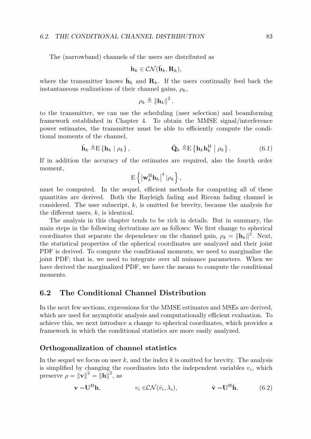
6.2. THE CONDITIONAL CHANNEL DISTRIBUTION 83
The (narrowband) channels of the users are distributed as
hk ∈ CN (hk,Rk),
where the transmitter knows hk and Rk. If the users continually feed back theinstantaneous realizations of their channel gains, ρk,
ρk � ‖hk‖2 ,to the transmitter, we can use the scheduling (user selection) and beamformingframework established in Chapter 4. To obtain the MMSE signal/interferencepower estimates, the transmitter must be able to efficiently compute the condi-tional moments of the channel,
hk �E {hk | ρk} , Qk �E{
hkhHk
∣∣ ρk} . (6.1)
If in addition the accuracy of the estimates are required, also the fourth ordermoment,
E{∣∣wH
k hk∣∣4 |ρk} ,
must be computed. In the sequel, efficient methods for computing all of thesequantities are derived. Both the Rayleigh fading and Ricean fading channel isconsidered. The user subscript, k, is omitted for brevity, because the analysis forthe different users, k, is identical.
The analysis in this chapter tends to be rich in details. But in summary, themain steps in the following derivations are as follows: We first change to sphericalcoordinates that separate the dependence on the channel gain, ρk = ‖hk‖2. Next,the statistical properties of the spherical coordinates are analyzed and their jointPDF is derived. To compute the conditional moments, we need to marginalize thejoint PDF; that is, we need to integrate over all nuisance parameters. When wehave derived the marginalized PDF, we have the means to compute the conditionalmoments.
6.2 The Conditional Channel Distribution
In the next few sections, expressions for the MMSE estimates and MSEs are derived,which are used for asymptotic analysis and computationally efficient evaluation. Toachieve this, we next introduce a change to spherical coordinates, which provides aframework in which the conditional statistics are more easily analyzed.
Orthogonalization of channel statisticsIn the sequel we focus on user k, and the index k is omitted for brevity. The analysisis simplified by changing the coordinates into the independent variables vi, whichpreserve ρ = ‖v‖2 = ‖h‖2, as
v =UHh, vi ∈CN (vi, λi), v =UHh, (6.2)

84 CHAPTER 6. MMSE SINR ESTIMATION WITH CGI FEEDBACK
whereR � UΛUH
is the eigenvalue decomposition of the channel covariance matrix, R, and
Λ � diag {λ1, . . . , λnT }
is diagonal with the eigenvalues ordered arbitrarily. The MMSE estimates of h andhhH are obtained from the estimates of v and vvH as
h =Uv, Qh =UQvUH, (6.3)
v �E{
v | ‖v‖2 = ρ}, Qv �E
{vvH | ‖v‖2 = ρ
}. (6.4)
The fourth order moment,E{∥∥wHh
∥∥4 ∣∣ ρ} ,which is used to compute the MSE, can also be expressed in the whitened coordi-nates:
E{∥∥wHh
∥∥4 ∣∣ ρ} = E{∥∥wHv
∥∥4 ∣∣ ρ}=
(vec(wwH)
)H E{
v∗vT ⊗ vvH∣∣∣ ρ} vec(wwH), (6.5)
where w � UHw. The second identity follows from (B.6) in Appendix B. The op-erators ⊗ and {·}∗ are the Kronecker product and conjucate operator, respectively,and vec(X) denotes the vector obtained by stacking the columns of X. The matrix,
E{
v∗vT ⊗ vvH∣∣∣ ρ} ∈ CnTnT×nTnT ,
represents the fourth order moment of v.
Spherical coordinates of CnT
The spherical parameterization of CnT used herein is obtained in two steps. Firsta cylindrical set of coordinates, based on ξi = |vi|2, is introduced and next thespherical radius is introduced in terms of ρ. The phases and element gains areseparated by the cylindrical coordinates defined as
vi =√ξi ejφi ∈ C⇐⇒ φi = ∠vi ∈ (−π, π]
ξi = |vi|2 ≥ 0.
The spherical radius, ρ = ‖v‖2, is related to ξi as ρ = ξ1 + · · · + ξnT . Tointroduce a spherical set of coordinates, we choose to parameterize ξnT in termsof ρ and ξ1, . . . , ξnT−1 as ξnT = ρ − (ξ1 + · · · + ξnT−1). Note that there is no lossof generality by choosing ξnT for the parameterization because the elements of v

6.2. THE CONDITIONAL CHANNEL DISTRIBUTION 85
can be ordered arbitrarily by the appropriate ordering of the columns of U. Insummary, the spherical coordinate change, v(ρ, ξnT−1,φ), is given by
vi =√ξi ejφi ∈ C, ∀i < nT
vnT =√ρ− 1TξnT−1 e
jφnT ∈ C⇐⇒
ρ ≥ 0ξnT−1 ≥ 0, 1TξnT−1 ≤ ρφi ∈ (−π, π] ∀i,
where ξm � [ξ1, . . . , ξm]T ∈ Rm+ is introduced for more compact notation. Notethat the chosen coordinates are not independent of each other, because they arecoupled by the bound 1TξnT−1 ≤ ρ. This has several consequences. For instance,
• The domain of the PDF of (ρ, ξnT−1,φ) is restricted by 1TξnT−1 ≤ ρ.• When integrating over elements in ξnT−1, the integration interval will depend
on the other elements.
The last point is addressed by specifying the integration order, such that we alwaysintegrate with respect to ξnT−1 first, next ξnT−2, and so on. For this, and otherpurposes, we define �m as the squared norm (radius) of v without the first m − 1components,
�m = �m(ρ, ξm−1) � ρ− (ξ1 + · · ·+ ξm−1) =∥∥∥[vm, . . . , vnT ]T
∥∥∥2. (6.6)
Note that �m should always be interpreted as a function of ρ, ξ1, . . . , ξm−1, evenwhen this is not explicitly stated in the sequel. The radius �m is useful becauseit provides the bound ξm + · · · + ξnT−1 ≤ �m. In particular, if ξi, i > m hasbeen removed by integration, then the integration interval for ξm will be given by0 ≤ ξm ≤ �m.
Statistical properties of the spherical coordinatesTo derive the MMSE estimates, v and Qv, it is necessary to find an expression forthe conditional PDF,
f(ξnT−1,φ|ρ) =f(ρ, ξnT−1,φ)f(ρ) , (6.7)
and, therefore, we proceed by establishing the joint PDF, f(ρ, ξnT−1,φ), in thefollowing lemma:
Lemma 6.1. The joint PDF of ρ, φ, and ξnT−1 is given by
f(ρ, ξnT−1,φ) = e−vHΛ−1v e− �nTλnT e
2√�nTλnT
{v∗nT ejφnT }2πλnT
nT−1∏i=1
e− ξiλi e
2√ξiλi{v∗i ejφi}
2πλi,
where �nT = �nT (ρ, ξnT−1) as defined in (6.6).

86 CHAPTER 6. MMSE SINR ESTIMATION WITH CGI FEEDBACK
Proof. The coordinate (ρ, ξnT−1,φ) is just a different parameterization of v ∈ CnT ;the PDF, f(ρ, ξnT−1,φ) can therefore be derived from the complex Gaussian PDFof v, which can be written as
fv(v) = e−vHΛ−1vnT∏i=1
e−|vi|
2
λi e2|vi|λi{v∗i ej∠vi}πλi
. (6.8)
We can express f(ρ, ξnT−1,φ) as
f(ρ, ξnT−1,φ) = fv(v(ρ, ξnT−1,φ)
) ∣∣∣∣ ∂(v,v�)∂(ρ, ξnT−1,φ)
∣∣∣∣ ,where � and � denote the real and imaginary parts of their complex arguments,respectively. The lemma follows by substituting to spherical coordinates in (6.8),and by noting that the Jacobian determinant is given by∣∣∣∣ ∂(v,v�)
∂(ρ,φ, ξnT−1)
∣∣∣∣ =∣∣∣∣∂(v,v�)∂(ξnT ,φ)
∣∣∣∣ ∣∣∣∣ ∂(ξnT )∂(ξnT−1, ρ)
∣∣∣∣=
(∣∣∣∣∂(v1 , v�1 )∂(ξ1, φ1)
∣∣∣∣)nT ∣∣∣∣ ∂(ξnT )∂(ξnT−1, ρ)
∣∣∣∣= 2−nT
∣∣∣∣det[
I 0−1T 1
]∣∣∣∣=2−nT .
It is useful to separate the dependence of the phases from ρ and ξnT−1;for instance, when we compute the MMSE estimates (6.4). The joint PDF of(ρ, ξnT−1,φ) can be expanded as
f(ρ, ξnT−1,φ) = f(ρ, ξnT−1) f(φ|ρ, ξnT−1), (6.9)
When computing the MMSE estimates we can thus first take the expectation withrespect to the phases—which can be done in closed form—and next proceed withthe more intricate integration with respect to ξnT−1 and ρ. The PDF, f(ρ, ξnT−1),can be expressed in closed form:
Lemma 6.2. The joint PDF of ρ and ξnT−1 can be expressed as
f(ρ, ξnT−1) = e−vHΛ−1ve− �nTλnT I0
(2 |vnT |λnT
√�nT
)λnT
nT−1∏i=1
e− ξiλi I0
(2 |vi|λi√ξi
)λi
, (6.10)
where �nT = �nT (ρ, ξnT−1) as defined in (6.6) and In (x) is the nth order modifiedBessel function (of the first kind).

6.2. THE CONDITIONAL CHANNEL DISTRIBUTION 87
Proof. The theorem follows from Lemma 6.1 and by applying Lemma 6.16 in Ap-pendix 6.C on
f(ρ, ξnT−1) =∫−π≤φi≤π, ∀i
f(ρ,φ, ξnT )dφ1 . . . dφnT .
The expansion in (6.9) is refined and fully characterized by the following lemma:
Lemma 6.3. The joint PDF of ρ, ξnT−1 and φ can be expanded as
f(ρ,φ, ξnT−1) = f(ρ, ξnT−1)nT∏i=1f(φi|ξi)
where
f(φi|ξi) = e2√ξiλi{v∗i ejφi}
2πI0(
2 |vi|λi√ξi
)and ξnT = �nT (ρ, ξnT−1), as defined in (6.6).
Proof. The conditional PDF, f(φ|ρ, ξnT−1), is obtained from Lemma 6.1 andLemma 6.2 as
f(φ|ρ, ξnT−1) =f(ρ, ξnT−1,φ)f(ρ, ξnT−1) = e
2√�nTλnT
{v∗nT ejφnT }
2πI0(
2|vnT |λnT
√�nT
) nT−1∏i=1
e2√ξiλi{v∗i ejφi}
2πI0(
2|vi|λi
√ξi
) .The lemma follows by expanding f(ρ,φ, ξnT−1) as in (6.9) and by identifying theconditional PDF, f(φi|ξi), in the preceding expression for f(φ|ρ, ξnT−1).
It is intuitive that the MMSE estimate,
|vn|2 = E {ξn | ρ}
is a monotonic increasing function in ρ; that is, if ‖v‖2 increases, then the MMSEestimates of the elements of v, also increases. This is established in the followingtheorem.
Theorem 6.4. Any conditional moment of ξn,
E {(ξn)s | ρ} , s > 0,
is a monotonic increasing function in ρ, for all n = 1, . . . , nT .

88 CHAPTER 6. MMSE SINR ESTIMATION WITH CGI FEEDBACK
Proof. Theorem 6.4 is easily proved by employing Lemmas 6.11 and 6.14, which weprove in Appendix 6.A. Define the stochastic variable,
b =∑j �=nξj .
By the definition of ρ, we have the equality, ρ = ξn + b. The stochastic variables,ξ1, . . . , ξnT , are independent; thus, b and ξn are independent. Moreover, the PDFof b is log-concave by Lemma 6.14 in Appendix 6.A and the PDFs of ξn and b areboth differentiable. Thus, according to Lemma 6.11
Pr {ξn > c | ρ}
is monotonic increasing in ρ. Any moment of ξn ≥ 0 can be written as [Dur96,Lemma (5.7)]
E {(ξn)s | ρ} =∫ ∞
0scs−1Pr {ξn > c | ρ} dc, s > 0.
The lemma follows, because the integrand in the preceding expression is a mono-tonic increasing function in ρ.
When taking expectations with respect to ξnT−1, typically just one or a few ξiare involved. A key contribution of this work is therefore the derivations of readilyevaluated expressions for the marginalized PDF,
f(ρ, ξm), m < nT ,
(of which f(ρ) is a special case), given in Theorem 6.5 (Rayleigh fading) andLemma 6.8 (Ricean Fading). For evaluation and simulation purposes, it is alsouseful to generate realizations of the conditional PDF (6.7). A factorization of themultivariate conditional PDF suitable for this is proposed in Appendix 6.B.
In the following discussion we assume that all eigenvalues of the covariancematrix, λ1, . . . , λnT , are distinct. In practice, this is not a limitation, since theeigenvalues are stochastic parameters depending on the environment of the prop-agation channel. In this setting, the eigenvalues are distinct almost surely. Thereason we limit the analysis to distinct eigenvalues is that every combination of twoor more equal eigenvalues must be treated as a separate case, which is not feasiblein this context.
6.3 Zero-Mean Channels
In this section we focus on the special case of zero-mean (Rayleigh fading) channels,which from an analytical perspective are more tractable than the general Riceanfading case. Closed form expressions for the MMSE estimates and the MSEs are

6.3. ZERO-MEAN CHANNELS 89
derived, and an asymptotic analysis is performed. With zero mean (i.e., v = 0) thejoint PDF of (ρ, ξnT−1,φ) is obtained from Lemma 6.1 as
f(ρ,φ, ξnT−1) =e− ρλnT
∏nT−1i=1 e
− ξiλi (1− λiλnT
)
(2π)nT λ1 . . . λnT. (6.11)
The PDF, f(ρ, ξnT−1), is obtained as
f(ρ, ξnT−1) =e− ρλnT
∏nT−1i=1 e
− ξiλi (1− λiλnT
)
λ1 . . . λnTξi ≥ 0 ∀i and 1TξnT−1 ≤ ρ, (6.12)
because f(ρ,φ, ξnT−1) is independent of φ
Marginalizing the PDFEven though the joint PDF in (6.12) does factor nicely in the random parameters,they remain coupled, and strongly dependent, because the domain of the PDF istightly coupled by the constraint 1TξnT−1 ≤ ρ. In order to derive the MMSEestimates, nuisance parameters are removed by integration. We define the partiallymarginalized joint PDF as
f(ρ, ξm) �∫
ξm+1+···+ξnT−1≤�m+1
f(ρ, ξnT−1) dξm+1 · · · dξnT
=∫ �m+1
0f(ρ, ξm+1) dξm+1.
The following theorem is important because it gives a closed form expression ofthe marginalized PDF. In the sequel, it is used to derive closed form expressionsfor the MMSE estimate of the received signal power,
∥∥wHh∥∥2. Furthermore, the
theorem also provides the means to derive the MSE of this estimator in closed form.Knowing the accuracy of the estimator is not only useful from an implementationperspective, as discussed in Section 4.2, but also from a theoretical perspective. Inparticular it allows for the asymptotic analysis in Section 6.4, where it is shownthat the MSE is in fact upper bounded by a constant, regardless of the size of ρ.
Theorem 6.5. For Rayleigh fading channels with distinct and non-zero eigenval-ues, λ1, . . . , λnT , the marginalized joint PDF, f(ρ, ξm), is given by
f(ρ, ξm) = 1∏mi=1 λi
nT∑k=m+1
e− ρλk
∏mi=1 e
− ξiλi (1− λiλk )
λknT∏i=m+1i�=k
(1− λiλk ), ξi ≥ 0 ∀i, 1Tξm ≤ ρ, (6.13)
for all m = 0, . . . , nT − 1.

90 CHAPTER 6. MMSE SINR ESTIMATION WITH CGI FEEDBACK
Proof. The proof is given in Appendix 6.D.
An important special case of Theorem 6.5 is the PDF of ρ,
f(ρ) =nT∑k=1
e− ρλk
λknT∏i=1i�=k
(1− λiλk ), (6.14)
which corresponds to m = 0. The PDF of ρ, which is a sum of the independentexponentially distributed variables ξi, has previously been analyzed in the field ofrenewal theory where ρ is related to the time to system failure. The PDF of ρ isfor instance found in [Cox62, page 17]. The conditional PDF f(ξm|ρ) is obtainedfrom Theorem 6.5 and (6.14) as
f(ξm|ρ) = f(ξm, ρ)f(ρ) ,
and in particular,
f(ξ1|ρ) = 1λ1f(ρ)
nT∑k=2
e− ρλk e− ξ1λ1
(1− λ1λk
)
λknT∏i=2i�=k
(1− λiλk ), (6.15)
which can be used to characterize the full PDF using Theorem 6.15 in Appendix 6.B.
Derivation of the MMSE estimatesNext, the MMSE estimates, v and Q, are derived using the marginalizedPDF (6.15). First observe that v = 0 and that Q is diagonal, because
vm = E {vm|ρ} = Eξm{√ξm Eφm
{ejφm
} ∣∣∣ ρ} = 0, ∀m
[Q]mn = E {vmv∗n|ρ} = Eξm,φm,ξn{√ξmξne
jφmEφn{e−jφn
} ∣∣∣ρ} = 0, m = n,(6.16)
where we use that the phases, φ, are uniformly distributed over [0, 2π], and remainindependent of the parameters ρ and ξnT−1.
Corollary 6.6. Let the elements of v be independent zero-mean complex Gaussianrandom variables, with distinct non-zero variances, λ1, . . . , λnT , then
v(ρ) = E{
v∣∣ ‖v‖2 = ρ
}= 0,
Q(ρ) = E{
vvH ∣∣ ‖v‖2 = ρ}
= Λ(ρ),

6.3. ZERO-MEAN CHANNELS 91
where Λ(ρ) is a diagonal matrix with elements [Λ(ρ)]mm = λm(ρ) given by
λm(ρ) = 1f(ρ)
[ ρ−nT∑k=1k �=m
λk
1− λkλm
λm∏i�=m
(1− λi
λm
)e− ρλm −
∑k �=m
e− ρλk(
1− λkλm)∏i�=k
(1− λiλk
)],(6.17)
where f(ρ) is the PDF of ρ = ‖v‖2, given by (6.14).
Proof. The proof is given is Appendix 6.E.
Fourth order momentsApart from the first and second order moments, also the fourth order moment ofv, are required to determine the accuracy of the estimates—that is, the MSE (4.8).The fourth order moment of v is given by the matrix
E{
v∗vT ⊗ vvH∣∣∣ ρ} ,
from which E{‖wHh‖4} is obtained as in (6.5). Due to the uniform phase distri-bution, which is preserved when conditioning on ρ for zero-mean channels, mostelements of the fourth order moment matrix are zero. An element of the momentmatrix is non-zero only if the complex phases cancel out—that is,
E {v∗i vjvmv∗n| ρ} = 0 only for (i = j & m = n) or (i = m & j = n).
The expression for E{‖wHh‖4| ρ} = E{‖wHv‖4| ρ} in (6.5) can therefore be sim-plified as
E{∥∥wHv
∥∥4 ∣∣ ρ} =(vec(wwH)
)H E{
v∗vT ⊗ vvH∣∣∣ ρ} vec(wwH)
=nT∑i=1|wi|4 E
{|vi|4
∣∣ ρ} + 4∑i>j
|wi|2 |wj |2 E{|vi|2 |vj |2
∣∣ ρ} .(6.18)
This can also be written in matrix form as
E{∥∥wHv
∥∥4 ∣∣ ρ} = pT T p,
where
[T]mn �{
E{ξ2m
∣∣ ρ} , m = n,2 E
{ξmξn
∣∣ ρ} , m = n,p �
[|w1|2 , . . . , |wnT |2]T.
The next corollary therefore completely characterizes the fourth order moment ofv by establishing T.

92 CHAPTER 6. MMSE SINR ESTIMATION WITH CGI FEEDBACK
Corollary 6.7. For Rayleigh fading channels with distinct and non-zero eigenval-ues, λ1, . . . , λnT , the second order moments of ξm are given by
E{ξ2m|ρ
}= e
− ρλm
f(ρ)
(ρ−∑
k �=mλk
1− λkλm
)2
+∑k �=m
λ2k(
1− λkλm)2
λm∏i�=m
(1− λi
λm
)+ 2f(ρ)
∑k �=m
λke− ρλk
(1− λkλm )2 ∏i�=k(1− λiλk )
, (6.19)
and
E {ξmξn|ρ} = 1f(ρ)
∑k �∈{m,n}
λke− ρλk
(1− λkλm )(1− λkλn )∏i�=k(1− λiλk )
+ e− ρλm
f(ρ)
λn − (1− λnλm )(ρ− ∑k �=m
λk
1− λkλm)
(1− λmλn )(1− λnλm )∏i�=m(1− λi
λm)
+ e− ρλn
f(ρ)
λm − (1− λmλn )(ρ− ∑k �=n
λk
1− λkλn)
(1− λnλm )(1− λmλn )∏i�=n(1− λiλn )
,
for all m,n ∈ {1, . . . , nT }, m = n.
Proof. The proof is given in Appendix 6.E.
Next, we use these results for an asymptotic analysis for large ρ.
6.4 Asymptotic Analysis
The reason that the MMSE SINR estimation framework with norm feedback,performs well in multiuser scenarios is best explained by the asymptotic behav-ior of the MMSE estimates. To simplify the notation in the following, we pre-sume, without loss of generality, that the elements of v are ordered such thatλ1 > λ2 > · · · > λnT > 0. The key observations are that for large ρ
• ξ1 = |v1|2 ≈ ρ− constant ≈ ρ• ξm = |vm|2 ≈ constant, m > 1
• The MSE of ξm = E {ξm| ρ} is upper bounded by a constant
• E{
(ξ1 − ρ)2∣∣ ρ} is upper bounded by a constant

6.4. ASYMPTOTIC ANALYSIS 93
These are interesting observations, and the very reason that a multiuser system withchannel norm feedback performs well; with many users, only users with large ρ arescheduled, and the preceding approximations apply. To show these observations,we first determine the asymptotic behavior of the conditional moments of ξm. ThePDF of ρ is given by (6.14), and the asymptotic behavior is seen to be
f(ρ) = e−ρλ1
λ1∏nTj=2(1− λjλ1
)
[1 +O
(e−
ρλ2
(1−λ2λ1
)) ]. (6.20)
The asymptotic behavior of the first order moment of ξm can be obtainedfrom (6.17) as
E {ξm|ρ} f(ρ) =
⎧⎪⎪⎨⎪⎪⎩ρ−∑nT
k=2λk
1−λkλ1
λ1∏nT
i=2(1− λiλ1
)e−
ρλ1
[1 +O
(e−
ρλ2
(1−λ2λ1
)) ], m = 1,
1( λ1λm−1)
∏nT
i=2(1− λiλ1
)e−
ρλ1
[1 +O
(e−
ρλ2
(1−λ2λ1
)) ], m = 1.
(6.21)Combining (6.20) and (6.21) yields
E {ξm|ρ} =
⎧⎪⎨⎪⎩(ρ−∑nT
k=2λk
1−λkλ1
)[1 +O
(e−
ρλ2
(1−λ2λ1
)) ], m = 1,
λm1−λmλ1
[1 +O
(e−
ρλ2
(1−λ2λ1
)) ], m = 1.
(6.22)
The asymptotics of E {ξm|ρ} give insight to the channel knowledge provided byρ, and (6.22) clearly shows how the characteristics of ξ1 differ from those of ξm,m > 1. It is interesting to note that E {ξ1|ρ} grow as ρ with a constant bias of
nT∑k=2
λk
1− λkλ1
for large ρ, whereas E {ξm|ρ}, m > 1 tends to the constant,
λm
1− λmλ1
.
Hence, for large ρ, Qh = E{
hhH∣∣ ρ} will be totally dominated by a single eigen-
mode of which the channel h must be closely aligned.This result can be further strengthened by considering higher order moments.
The asymptotics of the second order moment, E{ξ21 |ρ
}, are obtained from (6.19)
as
E{ξ21 |ρ
}=
⎡⎣(ρ− nT∑k=2
λk
1− λkλ1
)2
+nT∑k=2
λ2k(
1− λkλ1
)2
⎤⎦ [1 +O
(e−
ρλ2
(1−λ2λ1
)) ],

94 CHAPTER 6. MMSE SINR ESTIMATION WITH CGI FEEDBACK
0 1 2 3 4 5 60
1
2
3
4
5
6
ρ
ρ
E{|v1|2|ρ}RMSE
50% 90% 95% 98%
Figure 6.1: Illustrates the asymptotic behavior of the estimator E{|v1|2|ρ}. In thefigure nT = 3 and λi = e−(i−1). The vertical lines marked with 50%, 90%, 95%,and 98% represent the corresponding percentiles of ρ.
from which the MSE can be computed as
E{
(ξ1 − E {ξ1|ρ})2∣∣∣ ρ} = E
{ξ21 |ρ
}− (E {ξ1|ρ}
)2
=nT∑k=2
λ2k(
1− λkλ1
)2
[1 +O
(e−
ρλ2
(1−λ2λ1
)) ].
This is a strong result, because it states that the MSE of ξ1 = E {ξ1 | ρ} =E{|v1|2 | ρ} tends to a constant, even though E{|vi|2|ρ} tends to infinity. This isillustrated in Figure 6.1, where the estimator E{|v1|2|ρ} and the associated RMSEare displayed. As observed in the figure, the asymptotic behavior is apparent alsofor reasonable realizations of ρ. The bounded MSE also has the interesting conse-quence that the square distance between ρ and ξi is limited as
E{
(ξ1 − ρ)2∣∣∣ ρ} = E
{(ξ1 − E {ξ1|ρ}+ E {ξ1|ρ} − ρ)2
∣∣∣ ρ}= E
{(ξ1 − E {ξ1|ρ})2
∣∣∣ ρ} + (E {ξ1|ρ} − ρ)2
=
⎡⎣ nT∑k=2
λ2k(
1− λkλ1
)2 +(nT∑k=2
λk
1− λkλ1
)2⎤⎦ [
1 +O(e−
ρλ2
(1−λ2λ1
)) ].
(6.23)
If the beamformer, w, is fixed to the dominating unit norm eigenvector of R, thenξ1 is the received signal power. With optimized beamforming (with perfect CSI) the

6.5. CHANNELS WITH NON-ZERO MEAN 95
maximal achievable signal power is, ρ (achieved with w ∝ h). The relation (6.23)therefore states that the SNR loss of non-perfect CSI is bounded by a constant.The relative SNR loss (and thus the rate loss) therefore tends to zero. Hence, theperformance of fixed eigenbeamforming approaches that of perfect CSI when ρ islarge.
6.5 Channels with Non-Zero Mean
The analysis for the case with non-zero mean is more involved than for the zero-mean case. It is therefore not possible to derive closed form formulas for the PDF ofρ and for the conditional moments, in contrast to the case for zero-mean channels.However, it is possible to derive readily computable expressions for the aforemen-tioned quantities as shown below.
The PDFs and moments of interest, can all be expressed as convolutions of thefunctions
x(k,k)i (ξ) = e
− ξλi
λiξk
√ξkIk
(2 |vi|λi
√ξ
)u (ξ) , (6.24)
where k and k depend on the application,
u (x) � 12(1 + t|t| )
is the Heaviside step function and In (x) is the nth order, modified Bessel functionsof the first kind. We define y(k,k)
m (ρ) as the convolution of x(ki,ki)i (ξ), i ≥ m:
y(k,k)m (ρ) �
(�i≥mx
(ki,ki)i
)(ρ) (6.25)
�(x(km,km)m � x
(km+1,km+1)m+1 � · · · � x(knT ,knT )
nT
)(ρ).
The marginalized PDF, f(ξm, ρ)—the equivalent to Theorem 6.5 for Riceanchannels—is given by the next lemma:
Lemma 6.8. The marginalized PDF, f(ξm, ρ), can be expressed in terms ofy
(k,k)m (ρ) as
f(ξm, ρ) = e−vHΛ−1vy(0,0)m+1 (�m+1)
m∏i=1
e− ξiλi I0
(2 |vi|λi√ξi
)λi
, (6.26)
where �m+1 = ρ− ξ1 − · · · − ξm as in (6.6).
Proof. The marginalized PDF is, by definition, given by
f(ξm, ρ) �∫ξm+1+···+ξnT−1≤�m+1
f(ξnT−1, ρ)dξm+1 · · · dξnT−1,
which from Lemma 6.2 is recognized as the convolution in (6.25).

96 CHAPTER 6. MMSE SINR ESTIMATION WITH CGI FEEDBACK
As a special case of (6.26), the PDF of ρ is obtained as
f(ρ) = e−vHΛ−1vy(0,0)(ρ), (6.27)
where the notation y(k,k)(ρ) � y(k,k)1 (�1) is used for simplicity. Also the moments
of v can be expressed in terms of y(k,k)(ρ)
Lemma 6.9. Any moment of v for a given ‖v‖2 = ρ can be expressed in terms ofy(k,k)(ρ) � y(k,k)
1 (�1). For li, li ∈ N, i = 1, . . . , nT , it holds that
E{( nT∏i=1vlii (v∗i )li
)∣∣∣ρ} =( nT∏i=1
vli−lii
|vi|li−li)yk,k(ρ)y0,0(ρ) ,
whereki =
∣∣li − li∣∣ , ki = min{li, li}, ∀i.Proof. First take the expectation over the phases, for a given ξnT , as
E{( nT∏i=1vlii (v∗i )li
)∣∣∣ξnT}
=nT∏i=1
√ξi
=2ki+ki︷ ︸︸ ︷li + li
∫ πφi=−π
ej(li−li)φif(φi|ξi)dφi
(a)=( nT∏i=1
vli−lii
|vi|li−li) nT∏i=1
ξkii√ξikiIki
(2 |vi|λi√ρ)
I0
(2 |vi|λi√ρ)
(b)= e−vHΛ−1v
f(ξnT−1, ρ)
( nT∏i=1
vli−lii
|vi|li−li) nT∏i=1x
(ki,ki)i (ξi),
where f(φi|ξi) given in Lemma 6.2, Lemma 6.16, and the identity I−n (x) = In (x)for x ≥ 0 are used in (a). Equations (6.15) and (6.24) are used in (b). The Lemmafollows from
E{( nT∏i=1vlii (v∗i )li
)∣∣∣ρ} =
= 1f(ρ)
∫ξ1+···+ξnT−1≤ρ
E{( nT∏i=1vlii (v∗i )li
)∣∣∣ξnT}f(ξnT−1, ρ)dξ1 . . . dξnT−1
= 1y(0,0)(ρ)
( nT∏i=1
vli−lii
|vi|li−li)∫ξ1+···+ξnT−1≤ρ
nT∏i=1x
(ki,ki)i (ξi)dξ1 . . . dξnT−1,
because the integral is given, by definition, as yk,k(ρ). In the integrals above, ξnTis parameterized as ξnT = ρ− ξ1 − · · · − ξnT−1.
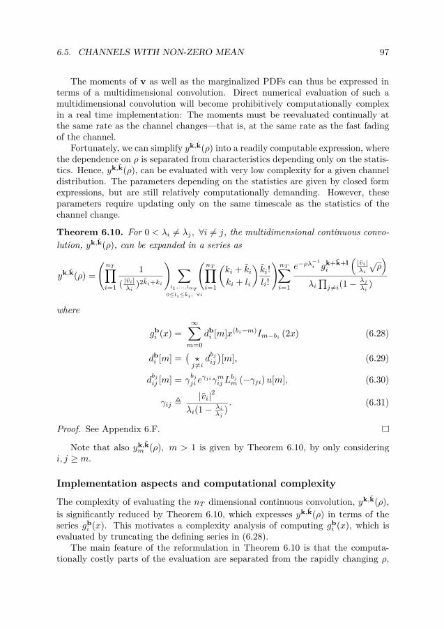
6.5. CHANNELS WITH NON-ZERO MEAN 97
The moments of v as well as the marginalized PDFs can thus be expressed interms of a multidimensional convolution. Direct numerical evaluation of such amultidimensional convolution will become prohibitively computationally complexin a real time implementation: The moments must be reevaluated continually atthe same rate as the channel changes—that is, at the same rate as the fast fadingof the channel.
Fortunately, we can simplify yk,k(ρ) into a readily computable expression, wherethe dependence on ρ is separated from characteristics depending only on the statis-tics. Hence, yk,k(ρ), can be evaluated with very low complexity for a given channeldistribution. The parameters depending on the statistics are given by closed formexpressions, but are still relatively computationally demanding. However, theseparameters require updating only on the same timescale as the statistics of thechannel change.
Theorem 6.10. For 0 < λi = λj , ∀i = j, the multidimensional continuous convo-lution, yk,k(ρ), can be expanded in a series as
yk,k(ρ) =(nT∏i=1
1( |vi|λi )2ki+ki
) ∑l1,...,lnT
0≤li≤ki, ∀i
(nT∏i=1
(ki + kiki + li
)ki!li!
)nT∑i=1
e−ρλ−1i gk+k+li
(|vi|λi
√ρ)
λi∏j �=i(1− λjλi )
where
gbi (x) =∞∑m=0dbi [m]x(bi−m)Im−bi (2x) (6.28)
dbi [m] =(�j �=idbjij
)[m], (6.29)
dbjij [m] = γbjji e
γjiγmijLbjm (−γji)u[m], (6.30)
γij � |vi|2λi(1− λiλj )
. (6.31)
Proof. See Appendix 6.F.
Note that also yk,km (ρ), m > 1 is given by Theorem 6.10, by only consideringi, j ≥ m.
Implementation aspects and computational complexity
The complexity of evaluating the nT dimensional continuous convolution, yk,k(ρ),is significantly reduced by Theorem 6.10, which expresses yk,k(ρ) in terms of theseries gbi (x). This motivates a complexity analysis of computing gbi (x), which isevaluated by truncating the defining series in (6.28).
The main feature of the reformulation in Theorem 6.10 is that the computa-tionally costly parts of the evaluation are separated from the rapidly changing ρ,

98 CHAPTER 6. MMSE SINR ESTIMATION WITH CGI FEEDBACK
and depend only on the slowly changing statistics and can therefore be precom-puted. More specifically, for precomputed dbi [m], the computational complexity ofevaluating gbi (x) is unaffected by nT and consequently the complexity of evaluatingyk,k(ρ) is linear in nT .
Evaluating gbi (x)
For precomputed dbi [m], the truncated series
gbi (x) =M−1∑m=0dbi [m]x(bi−m)Im−bi (2x)
can be evaluated without explicitly computing the Bessel functions in each term.Each term in the sum is readily evaluated recursively (starting with m = M −1), because the Bessel functions satisfy the following backwards stable recurrencerelation:
In+1 (x) = In−1 (x)− 2nxIn (x) ,
see for example [AS72, 9.6.26].The initial points in the Bessel function recursion, IM−bi (2x) and IM+1−bi (2x),
can be obtained (up to a scaling) by using the backwards stability of the recurrenceand starting the backwards recursion at m > M with an arbitrary initialization ofthe recursion, see [PTVF92].
Computing dbi [m] recursively
Even though the parameters dbi [m] depend only on the statistics of the channel(i.e., they do not require rapid updating) the computational complexity of thenT − 1 dimensional convolution becomes considerable for large nT . Fortunately,it is sufficient to compute d0i [m], from which dbi [m] can be obtained by using therecurrence relation,
db+eji [m] = γjidbi [m] + γijd
b+eji [m− 1],
where ej is the vector where only the jth element is non-zero and equal to 1. Thisrecurrence relation follows by expanding the definition of dbi [m] in (6.29) with thefollowing recurrence relation of generalized Laguerre polynomials:
Lk+1n (x) = Lkn (x) + Lk+1
n−1 (x) ,
see for example [AS72, 22.7.30].
6.A Lemmas for Proof of Theorem 6.4
Lemma 6.11. Let a and b be stochastic, independent, and have differentiable PDFsfA(a) and fB(b), respectively. If fB(b) is log-concave in b, then Pr {a ≥ c|a+ b = ρ}is increasing in ρ.

6.A. LEMMAS FOR PROOF OF THEOREM 6.4 99
Proof. 1 Define
h(ρ) � Pr {a ≥ c | a+ b = ρ} =∫∞cfA(x)fB(ρ− x)dx∫∞
−∞ fA(x)fB(ρ− x)dx,
where the identity follows by noting that the joint PDF fA,ρ(a, ρ) = fA,B(a, ρ−a) =fA(a)fB(ρ− a). Differentiate with respect to ρ to get
h′(ρ) = 1(·)2
[ ∫ ∞c
fA(x)f ′B(ρ− x)dx∫ ∞−∞fA(x)fB(ρ− x)dx
−∫ ∞c
fA(x)fB(ρ− x)dx∫ ∞−∞fA(x)f ′B(ρ− x)dx
]= 1
(·)2
[ ∫x≥c,y
g(x, y)dxdy −∫y≥c,x
g(x, y)dxdy],
where g(x, y) � fA(x)fA(y)f ′B(ρ−x)fB(ρ− y), and the denominator (·)2 is strictlypositive. The two integrals cancel over the area where both x > c and y > c, andthus
h′(ρ) = 1(·)2
[ ∫x≥c,c≥y
g(x, y)dxdy −∫y≥c,c≥x
g(x, y)dxdy]
= 1(·)2
∫x≥c,c≥y
[g(x, y)− g(y, x)]dxdy
It follows that h′(ρ) is non-negative, because the integrand is non-negative in theintegration domain:
g(x, y)− g(y, x) = fA(x)fA(y) [f ′B(ρ− x)fB(ρ− y)− f ′B(ρ− y)fB(ρ− x)]︸ ︷︷ ︸(�)
.
It follows by the log-concavity assumption on fB(b), that (�) is non-negative when-ever x ≥ y (as in the integration domain), because with log-concave fB(b),
∂
∂blog fB(b) = f
′B(b)fB(b)
is a monotonic decreasing function.
Lemma 6.12. If ν ≥ 0, then Iν (√x) is strictly log-concave in x ≥ 0.
Proof. Baricz and Neuman [BN07] have proved that Iν (√x) is strictly log-concave
for ν > 0. It thus remains to consider the case ν = 0, which is of more interest
1I would like to thank Dr. Joakim Jaldén for his contributions to the proof of Lemma 6.11.

100 CHAPTER 6. MMSE SINR ESTIMATION WITH CGI FEEDBACK
herein. It can be shown that I0 (√x) is strictly log-concave using straightforward
modifications of the proof in [BN07], but for completeness we give a proof next.The function, I0 (
√x), is log-concave if the derivative of log I0 (
√x) is a strictly
decreasing function in x. The derivative is obtained as
∂
∂xlog I0
(√x)
=∂∂xI0 (
√x)
I0 (√x)
= 12I1 (√x)√
xI0 (√x)
= 12f(√x),
where we have definedf(x) � x
−1I1 (x)I0 (x) .
Thus, I0 (√x) is strictly log-concave if and only if f(x) is a strictly decreasing
function for x ≥ 0. The derivative of f(x) is obtained as follows:
f ′(x) =∂∂x
1xI1 (x)I0 (x) −
1xI1 (x)I0 (x)2
∂
∂xI0 (x) =
I0 (x) I2 (x)− (I1 (x)
)2
x(I0 (x)
)2 , (6.32)
where we have used the relations [Pou99]:
∂
∂xx−νIν (x) = x−νIν+1 (x) , (6.33)
∂
∂xI0 (x) = I1 (x) . (6.34)
Using Amos’ inequality [Amo74],
Iν (x) Iν+2 (x)− (Iν+1 (x)
)2(Iν+1 (x)
)2 < 0, x ≥ 0,
and by noting that for n ∈ Z, it holds that 0 < x(In (x)
)2<∞ for 0 < x <∞, we
see from (6.32) thatf ′(x) < 0, x > 0.
Note that f ′(x) is continuous and well behaved about x = 0, and f ′(0) = 0.It follows that f(x) is strictly monotone decreasing for x ≥ 0, which proves thelemma.
Lemma 6.13. The PDF of ξj,
f(ξj) = e−|vj |
2
λj
λje− ξjλj I0
(2 |vj |λj
√ξj
),
is a log-concave function in ξj.
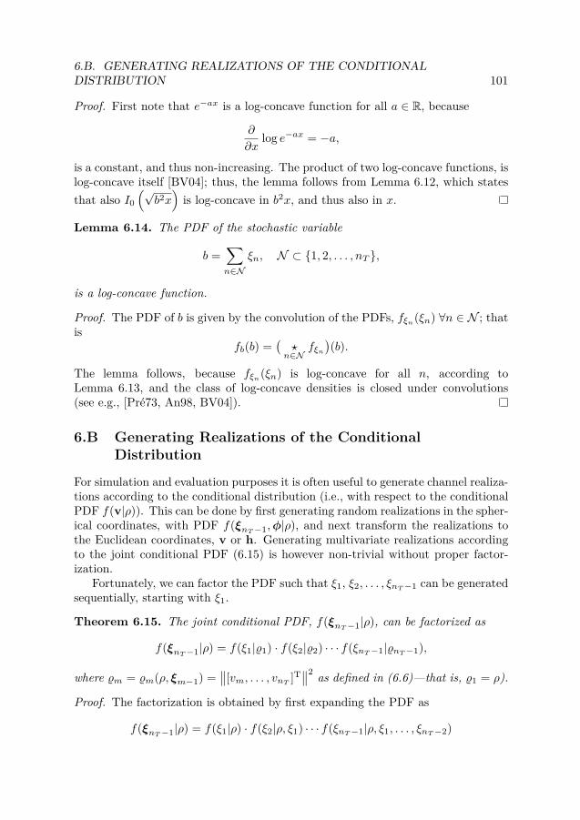
6.B. GENERATING REALIZATIONS OF THE CONDITIONALDISTRIBUTION 101
Proof. First note that e−ax is a log-concave function for all a ∈ R, because
∂
∂xlog e−ax = −a,
is a constant, and thus non-increasing. The product of two log-concave functions, islog-concave itself [BV04]; thus, the lemma follows from Lemma 6.12, which statesthat also I0
(√b2x
)is log-concave in b2x, and thus also in x.
Lemma 6.14. The PDF of the stochastic variable
b =∑n∈Nξn, N ⊂ {1, 2, . . . , nT },
is a log-concave function.
Proof. The PDF of b is given by the convolution of the PDFs, fξn(ξn) ∀n ∈ N ; thatis
fb(b) =(�n∈Nfξn
)(b).
The lemma follows, because fξn(ξn) is log-concave for all n, according toLemma 6.13, and the class of log-concave densities is closed under convolutions(see e.g., [Pré73, An98, BV04]).
6.B Generating Realizations of the ConditionalDistribution
For simulation and evaluation purposes it is often useful to generate channel realiza-tions according to the conditional distribution (i.e., with respect to the conditionalPDF f(v|ρ)). This can be done by first generating random realizations in the spher-ical coordinates, with PDF f(ξnT−1,φ|ρ), and next transform the realizations tothe Euclidean coordinates, v or h. Generating multivariate realizations accordingto the joint conditional PDF (6.15) is however non-trivial without proper factor-ization.
Fortunately, we can factor the PDF such that ξ1, ξ2, . . . , ξnT−1 can be generatedsequentially, starting with ξ1.
Theorem 6.15. The joint conditional PDF, f(ξnT−1|ρ), can be factorized as
f(ξnT−1|ρ) = f(ξ1|�1) · f(ξ2|�2) · · · f(ξnT−1|�nT−1),
where �m = �m(ρ, ξm−1) =∥∥[vm, . . . , vnT ]T
∥∥2 as defined in (6.6)—that is, �1 = ρ).
Proof. The factorization is obtained by first expanding the PDF as
f(ξnT−1|ρ) = f(ξ1|ρ) · f(ξ2|ρ, ξ1) · · · f(ξnT−1|ρ, ξ1, . . . , ξnT−2)

102 CHAPTER 6. MMSE SINR ESTIMATION WITH CGI FEEDBACK
and by noting that
f(ξm|ρ, ξ1, . . . , ξm−1) = f(ξm|�m, ξ1, . . . , ξm−1) = f(ξm|�m).
The first equality above follows because the conditioning has the same information(i.e., ρ = �m+ξ1+· · ·+ξm−1). The second equality follows from the independence ofthe elements of v, because this implies that ξm = |vm|2 and �m =
∥∥[vm, . . . , vnT ]T∥∥2
are both independent of ξi = |vi|2 ∀i < m.
This factorization is useful because f(ξi|�i) has the same form as f(ξ1, ρ),
f(ξi|�i) = f(|vi|2∣∣ ∥∥[vi, . . . , vnT ]T
∥∥2 = �i),
and is given by considering only the last nT − i + 1 elements of v in (6.15) and(6.26) for Rayleigh and Ricean fading, respectively. For Rayleigh fading, the PDFis obtained as
f(ξi|�i) = 1λif(�i)
nT∑k=i+1
e− �iλk e−
ξiλi
(1− λiλk )
λknT∏n=i+1n �=k
(1− λnλk ). (6.35)
Hence if ξ1 is first realized from the PDF f(ξ1|ρ), then ξ2 can next be realizedfrom the PDF f(ξ2|�2 = ρ − ξ1). Similarly ξi for i > 2 is realized by continuingthe iteration. Furthermore, as ξi is realized, φi can also be realized because it isindependent of all other parameters according to Lemma 6.2.
6.C Lemmas for the Derivations of Conditional PDFs
Lemma 6.16. If n ∈ Z, α ∈ R, and v ∈ C, then∫ π−πejnφeα{v∗ejφ}dφ = 2π v
n
|v|n In (α |v|) . (6.36)
Proof. ∫ π−πejnφeα{v∗ejφ}dφ = ejn∠v
∫ π−πejn(φ−∠v)eα|v|{ej(φ−∠v)}dφ
(a)= ejn∠v∫ π−π
cos(nφ)eα|v| cos φdφ
where in (a), φ = φ − ∠v and the imaginary part of the integral is zero, due tosymmetry. The last expression is identified in [AS72, 9.6.19], from which the lemmafollows.

6.C. LEMMAS FOR THE DERIVATIONS OF CONDITIONAL PDFS 103
Lemma 6.17. If σ1, . . . , σn, are distinct and positive, thenn∑k=1
1σmk
∏ni=1i�=k
(1− σiσk
) =δ[m],
for all m = 0, . . . , n− 1.
Proof. Denote the sum G(σ,m, n). For m = 0, the identity can be proved by thepartial fraction expansion
n∏k=1
11 + σkt
=n∑k=1
1
(1 + σkt)n∏i=1i�=k
(1− σiσk ). (6.37)
It follows from (6.37) that
G(σ,m = 0, n) = limt→0
n∏k=1
1/(1 + σkt) = 1, n > 0.
Similarly, G(σ,m = 1, n) follows also from the partial fraction (6.37) as
G(σ,m = 1, n) = limt→∞ t
n∏k=1
1/(1 + σkt) = 0, n > 1.
Next, an induction step for m > 0 is established.
G(σ,m− 1, n) =n∑k=1
1σm−1k
∏ni=1i�=k
(1− σiσk )
=n−1∑k=1
1σm−1k (1− σnσk )
∏n−1i=1i�=k
(1− σiσk )+ 1σm−1n
∏n−1i=1 (1− σiσn )
(a)=n−1∑k=1
1σm−1k
∏n−1i=1i�=k
(1− σiσk )
+n−1∑k=1
σnσk
σm−1k (1− σnσk )
∏n−1i=1i�=k
(1− σiσk )+ 1σm−1n
∏n−1i=1 (1− σiσn )
=G(σ,m− 1, n− 1) + σnG(σ,m, n),
where the identity
1(1− σnσk ) =
1− σnσk + σnσk
(1− σnσk ) = 1 + σnσk(1− σnσk )

104 CHAPTER 6. MMSE SINR ESTIMATION WITH CGI FEEDBACK
was used in (a). The result can be written as
G(σ,m, n) = 1σn
[G(σ,m− 1, n)−G(σ,m− 1, n− 1)
](6.38)
Assume that G(σ,m, n) = δ[m] holds for m =M −1, ∀n ≥M ; then it follows that
G(σ,M − 1, n) = G(σ,M − 1, n− 1), ∀n > M.It follows from (6.38) that G(σ,M, n) = 0,∀n > M > 0. Lemma 6.17 follows byinduction.
6.D Proof of Theorem 6.5
Proof. Assume (6.13) holds for m =M > 0, then f(ρ, ξM−1) can be derived as
f(ρ, ξM−1) =∫ �M
0f(ρ, ξM ) dξM
= 1∏Mi=1 λi
nT∑k=M+1
e− ρλk (
∏M−1i=1 e
− ξiλi (1− λiλk ))∫ �M
0 e− ξMλM (1−λMλk )
dξM
λknT∏
i=M+1i�=k
(1− λiλk )
(a)= 1∏M−1i=1 λi
[nT∑
k=M+1
e− ρλk (
∏M−1i=1 e
− ξiλi (1− λiλk ))
λknT∏i=Mi�=k
(1− λiλk )
−nT∑
k=M+1
e− ρλM
∏M−1i=1 e
− ξiλi (1− λiλM
)
λknT∏i=Mi�=k
(1− λiλk )
]
(b)= 1∏M−1i=1 λi
nT∑k=M
e− ρλk
∏M−1i=1 e
− ξiλi (1− λiλk )
λknT∏i=Mi�=k
(1− λiλk ),
where (a) follows from (6.6) and straightforward integration, and (b) follows fromLemma 6.17 in Appendix 6.C as
−nT∑
k=M+1
1
λknT∏i=Mi�=k
(1− λiλk )= −
nT∑k=M
1
λknT∏i=Mi�=k
(1− λiλk )
︸ ︷︷ ︸=0
+ 1
λMnT∏
i=M+1(1− λi
λM). (6.39)
Hence, if (6.13) holds for m =M , then it also holds for m =M − 1. The theoremfollows by induction, because (6.13) holds for m = nT − 1 according to (6.12).

6.E. PROOFS OF COROLLARIES 105
6.E Proofs of Corollaries
Lemma 6.18. If σ1, . . . , σn are distinct and positive, then
n∑k=1k �=m
1(1− σkσm
)∏ni=1i�=k
(1− σiσk
) =
∑nk=1k �=m
11−σmσk∏n
i=1i�=m
(1− σi
σm
) , (6.40)
and
n∑k=1k �=m
σk(1− σkσm
)2 ∏ni=1i�=k
(1− σiσk
) =− σm2
∑nk=1k �=m
1(1−σmσk )2 +
(∑nk=1k �=m
11−σmσk
)2
∏ni=1i�=m
(1− σi
σm
) . (6.41)
Proof. To prove the identities, the following Taylor expansion is useful. The firstequality follows from (6.37).
n∑k=1k �=m
1(1 + σkt
)∏ni=1i�=k
(1− σiσk
) = 1∏ni=1
(1 + σit
) − 1(1 + σmt)
∏ni=1i�=m
(1− σi
σm
)=
∏ni=1
(1− σi
σm
)−∏ni=1i�=m
(1 + σit
)(1 + σmt)
∏ni=1i�=m
(1− σi
σm
)︸ ︷︷ ︸
(�)
× 1∏ni=1i�=m
(1 + σit
)︸ ︷︷ ︸
(��)
(a)=
∑nk=1k �=m
11−σmσk∏n
i=1i�=m
(1− σi
σm
) + 12
∑nk=1k �=m
1(1−σmσk )2 +
(∑nk=1k �=m
11−σmσk
)2
∏ni=1i�=m
(1− σi
σm
) (1 + σmt)+
+O (1 + σmt)2, (6.42)
where (a) follows by expanding the factors (�) and (��) in Taylor series aboutt = −σ−1
m and collect the terms. The identities (6.40) and (6.41) follow by notingthat
n∑k=1k �=m
σqk(1− σkσm
)q+1 ∏ni=1i�=k
(1− σiσk
) = (−1)q
q! limt→σ−1
m
∂q
∂tq
n∑k=1k �=m
1(1 + σkt
)∏ni=1i�=k
(1− σiσk
)

106 CHAPTER 6. MMSE SINR ESTIMATION WITH CGI FEEDBACK
Proof of Corollary 6.6
Proof. First note that Q(ρ) is diagonal, by (6.16). The first diagonal entry of Q(ρ)is derived as
λ1 = E {ξ1|ρ} =∫ ρ
0ξ1f(ξ1|ρ) dξ1 = 1
λ1f(ρ)
nT∑k=2
e− ρλk
∫ ρ0 ξ1e
− ξ1λ1
(1− λ1λk
)dξ1
λkn∏i=2i�=k
(1− λiλk )
= 1f(ρ)
nT∑k=2
e− ρλk − e− ρ
λ1
(λkλ1− 1)
n∏i=1i�=k
(1− λiλk )− 1f(ρ)
nT∑k=2
ρe−ρλ1
λkn∏i=1i�=k
(1− λiλk )
= 1f(ρ)
⎡⎢⎢⎢⎢⎢⎣ρ+ λ1
∑nTk=2
11− λ1
λk
λ1∏ni=2(1− λiλ1
)e−
ρλ1 −
nT∑k=2
e− ρλk
(1− λkλ1)n∏i=1i�=k
(1− λiλk )
⎤⎥⎥⎥⎥⎥⎦ ,
where the last identity follows from Lemmas 6.17 and 6.18, similar to (6.39). Theexpression (6.17) follows from symmetry, because the ordering of v, and thus thatof λi, is arbitrary.
Proof of Corollary 6.7
Proof. We first derive E{|v1|4 |ρ}, from which E{|vm|4 |ρ}, for arbitrary m, followsby symmetry.
E{|v1|4 |ρ
}=∫ ρ
0ξ21f(ξ1|ρ) dξ1 = 1
λ1f(ρ)
nT∑k=2
e− ρλk
∫ ρ0 ξ
21e− ξ1λ1
(1− λ1λk
)dξ1
λkn∏i=2i�=k
(1− λiλk )=
(a)= 1f(ρ)
nT∑k=2
⎡⎢⎢⎢⎢⎢⎣−(�)︷ ︸︸ ︷ρ2e−
ρλ1
λkn∏i=1i�=k
(1− λiλk )+
(��)︷ ︸︸ ︷2ρe−
ρλ1
(1− λkλ1)n∏i=1i�=k
(1− λiλk )+ 2(e−
ρλk −
(���)︷ ︸︸ ︷e−
ρλ1 )
1λk
(1− λkλ1)2 ∏
i�=k(1− λiλk )
⎤⎥⎥⎥⎥⎥⎦
(b)=
(ρ−∑nT
k=2λk
1−λkλ1
)2
+∑nTk=2
λ2k(
1−λkλ1
)2
f(ρ) λ1∏ni=2
(1− λiλ1
) e−ρλ1 + 2
f(ρ)
nT∑k=2
λke− ρλk
(1− λkλ1)2 ∏
i�=k(1− λiλk ),

6.F. PROOF OF THEOREM 6.10 107
where (a) follows by straightforward integration, and (b) follows by applyingLemma 6.17 on (�), and by applying (6.40) and (6.41) of Lemma 6.18 on (��)and (� � �), respectively. Similarly, E{|v1|2 |v2|2 |ρ} is obtained as
E{|v1|2 |v2|2 |ρ
}=
∫ ρ0ξ1
∫ ρ−ξ10
ξ2f(ξ1, ξ2|ρ) dξ2 dξ1
(a)= 1f(ρ)
nT∑k=3
λke− ρλk
(1− λkλ1)(1− λkλ2
)∏i�=k(1− λiλk )
+ e− ρλ1
f(ρ)
λ2 − (1− λ2λ1
)(ρ− ∑k �=1
λk
1−λkλ1
)
(1− λ1λ2
)(1− λ2λ1
)∏i�=1(1− λiλ1
)
+ e− ρλ2
f(ρ)
λ1 − (1− λ1λ2
)(ρ− ∑k �=2
λk
1−λkλ2
)
(1− λ2λ1
)(1− λ1λ2
)∏i�=2(1− λiλ2
),
where (a) follows by tedious, but straightforward, integration, and by applyingLemma 6.17 and (6.40) of Lemma 6.18 on all applicable terms, similar to thederivations of E{|v1|4 |ρ}. Corollary 6.7 follows by symmetry.
6.F Proof of Theorem 6.10
The outline of the proof is as follows. First the convolution, defining yk,k(ρ), isdecoupled by means of Laplace transformation. The Laplace transform,
Y k,k(s) � L{yk,k(ρ)
},
is derived in closed form. Finally the Laplace transform is inverted by deriving theresidues of Y k,k(s).
Transformation to the Laplace domain
By the convolution property of Laplace transforms, Y k,k(s), is given by
Y k,k(s) = X(k1,k1)1 (s)X(k2,k2)
2 (s) · · ·X(knT ,knT )nT (s), (6.43)
whereX
(k1,k1)1 (s) � L
{x
(ki,ki)i (ρ)
}is the Laplace transform of x(ki,ki)
i (ρ). To derive X(k1,k1)1 (s) we need the following
lemma.

108 CHAPTER 6. MMSE SINR ESTIMATION WITH CGI FEEDBACK
Lemma 6.19. The Taylor expansion of s−(k+1)eαs about s = s = 0 is given by
eαs
sk+1 = eαs
sk+1
∞∑n=0
(−s)−nLkn(−αs
)(s− s)n, (6.44)
where Lkn (x) are generalized Laguerre polynomials.
Proof. First expand the function as
eαs
sk+1 = eαs
sk+1eαs [ ss−1]
( ss )k+1 = eαs
sk+1
(�)︷ ︸︸ ︷eαs [
s−ss
1− s−ss
]
(1− s−ss )k+1 .
The lemma follows by identifying (�) as the generating function of generalizedLaguerre polynomials [AS72, 22.9.15].
Lemma 6.20. The Laplace transform of x(ki,ki)i (ρ) is given by
X(ki,ki)i (s) =
ki∑li=0
ki!li!
(ki + kiki + li
) ( |vi|λi )2li+ki
λi
e
|vi|2λ2i
(s+λ−1i
)
(s+ λ−1i )ki+ki+li+1
.
Proof.
X(ki,ki)i (s) = L
{x
(ki,ki)i (ξ)
} (a)= (−1)kiλi
∂ki
∂skiL{√ξkIk
(2 |vi|λi
√ξ
)u (ξ)
} ∣∣∣s←s+ 1
λi
(b)= (−1)kiλi
( |vi|λi
)ki ∂ki
∂ski
⎛⎜⎜⎝ e
|vi|2λ2i
(s+ 1λi
)
(s+ 1λi
)ki+1
⎞⎟⎟⎠(c)=ki! ( |vi|λi )ki e
|vi|2λ2i
(s+λ−1i
)
λi (s+ λ−1i )ki+ki+1
Lkiki
(− |vi|2λ2i (s+ 1
λi)
),
where (a) follows from the Laplace transform relation,
L{tke−αtf(t)} = ∂
∂skF (s+ α),
(b) follows by identifying the Laplace transform [AS72, 29.3.81], and (c) follows byidentifying the derivative in the Taylor series in Lemma 6.19. The lemma followsby expanding the Laguerre polynomial explicitly [AS72, 22.3.9].

6.F. PROOF OF THEOREM 6.10 109
By combining (6.43) and Lemma 6.20 the next lemma is obtained, which givesY (k,k)(s) in closed form.
Lemma 6.21. Y (k,k)(s) is given by
Y (k,k)(s) =∑
l1,...,lnT0≤li≤ki, ∀i
[nT∏i=1
ki!li!
(ki + kiki + li
)]Y (l,k,k)(s),
where
Y (l,k,k)(s) �nT∏i=1
( |vi|λi )2li+ki
λi
e
|vi|2λ2i
(s+λ−1i
)
(s+ λ−1i )ki+ki+li+1
.
Transformation to the original domain
It follows from Lemma 6.21 that yk,k(s) can be computed from
y(l,k,k)(ρ) =L−1{Y (l,k,k)(s)
}=nT∑i=1
Res[Y (l,k,k)(s)eρs, s = −λ−1
i
], (6.45)
where Res [Y (s), s = α] denotes the residue of Y (s) at s = α. The problem of com-puting y(k,k)(ρ) has thus been reduced to computing the residues of Y (l,k,k)(s)eρs.
Consider the residue of Y (l,k,k)(ρ)eρs at s = −λ−1i . The residue is obtained
from the Laurent expansion of Y (l,k,k)(ρ)eρs about s = −λ−1i , or more specifically
by the term corresponding to (s + λ−1i )−1 in the expansion. The Laurent/Taylor
expansions of each factor of Y (l,k,k)(ρ)eρs is next derived, from which the jointexpansion is obtained. Only one factor of Y (l,k,k)(ρ)eρs is singular at s = −λ−1
i ,and its Laurent expansion is considered in the next lemma.
Lemma 6.22.
e
|vi|2λ2i
(s+λ−1i
) eρs
(s+ λ−1i )bi+1 = e−
ρλi
∞∑m=−∞
cm(s+ λ−1i )m,
where
cm �(√ρλi
|vi|)m+bi+1
Im+bi+1
(2 |vi|λi
√ρ
).
Proof. First note that
eαs+βs = e
√αβ
[1√βαs
+√
βα s
]︸ ︷︷ ︸
(�)
(a)=∞∑
n=−∞
(βα
)n2In
(2√αβ
)sn,

110 CHAPTER 6. MMSE SINR ESTIMATION WITH CGI FEEDBACK
where (a) follows by identifying (�) as the generating function of the modified Besselfunctions [AS72, 9.6.33]. The lemma follows by applying this result on
e
|vi|2λ2i
(s+λ−1i
) eρs
(s+ λ−1i )bi+1 = e
− ρλi
(s+ λ−1i )bi+1 e
|vi|2λ2i
(s+λ−1i
)+ρ(s+λ−1)
The other factors of Y (l,k,k)(s)eρs can be expanded in a Taylor series abouts = −λ−1
i .
Lemma 6.23.
∏j �=i
e
|vj |2λ2j
(s+γ−1j
)
(s+ γ−1j )bj+1 =
⎛⎜⎝∏j �=i
( |vj |2λ2j
)−bjλ−1j − λ−1
i
⎞⎟⎠ ∞∑m=0
( |vi|2
λ2i
)−m dbi [m] (s+ λ−1i )m,
where dbi [m] is defined in (6.29).
Proof. First consider a single factor of the product. By applying Lemma 6.19 itcan be expanded as
e
|vj |2λ2j
(s+γ−1j
)
(s+ γ−1j )bj+1 = e
|vj |2λj(1−
λjλi
)
(λ−1j − λ−1
i )bj+1
∞∑m=0
Lbjm
(− |vj |2λj(1−λjλi )
)(λ−1i − λ−1
j )m(s+ λ−1
i )m
=
( |vj |2λ2j
)−bjλ−1j − λ−1
i
∞∑m=0
( |vi|2
λ2i
)−m dbij [m] (s+ λ−1i )m,
where dbij [m] is defined in (6.29). Thus, with dbi [m] � �j �=idbij [m], the lemma follows.
The residue of Y (k,k)(s)eρs at s = −λ−1i (i.e., the weight of (s + λ−1
i )−1 inthe Laurent expansion of Y (k,k)(s)eρs) is finally obtained from Lemma 6.22 and

6.F. PROOF OF THEOREM 6.10 111
Lemma 6.23 as
Res[Y (l,k,k)(s)eρs, s = −λ−1
i
]=
=
⎛⎝ nT∏j=1
( |vj |λj )2li+ki
λi
⎞⎠ e−ρλ−1i
∏j �=i
( |vj |2λ2j
)−bjλ−1j − λ−1
i
∞∑m=0
( |vi|2
λ2i
)−m dbi [m]c−m−1
= 1∏nTi=1( |vi|λi )2ki+ki
(e− ρλi
λi∏j �=i(1− λjλi )
)×
×∞∑m=0dbi [m]
(√ρ |vi|λi
)bi−mI|m−bi|
(2 |vi|λi
√ρ
), (6.46)
where bi = ki + ki + li. Theorem 6.10 follows by combining Lemma 6.21, (6.45),and (6.46).


Chapter 7
Performance Evaluation
In this chapter we evaluate the performance of a system that uses the proposedMMSE SINR estimation framework to utilize CDI and CGI (i.e., ρk = ‖hk‖2) forthe resource scheduling. Consider a single cell, where the base station is equippedwith a uniform circular array (UCA) of transmit antennas. The diameter of thearray is set to 1 wavelength. The performance of the MMSE SINR estimationframework, when combined with various beamforming/user-selection schemes dis-cussed in the previous chapters, is evaluated in terms of cell (system) throughputor in terms of user throughput.
In all considered schemes, the user selction is made according to the greedyapproach given in Table 4.1. The channel is modeled as block fading, and in eachblock a single set of users is scheduled using the proportional fair criterion [KMT97,VTL02], where the short term average throughput of each user is evaluated usingan exponentially weighted low pass filter, ∝ exp(−t/a), where a = 100 blocks.
We consider a narrowband, flat-fading, propagation channel:
hk ∈ CN (hk,Rk).
Note, however, that the performance results apply also in wideband OFDM sys-tems, where each subcarrier is narrowband and can be treated separately. Thecovariance matrix of the channel fading, Rk, was computed using the assumptionof Gaussian distributed scattering with angular spread σθ (standard deviation ofthe distribution) [ZO94b]. If not stated otherwise, we consider a Rayleigh fadingchannel, with
σθ = 10 degrees,
which is typical for wide-area scenarios [PMF98, APM02, JZOG07]. Note thatthis corresponds to an angular spread sector of 2σθ = 20 degrees. For Riceanfading channels, the mean component, hk, is aligned with the array response in thedirection of the user.
A circular cell is considered, and the users are randomly positioned within thecell (with a uniform distribution), but not closer to the base station than 20 percent
113

114 CHAPTER 7. PERFORMANCE EVALUATION
of the cell radius. A realization of the user positions is denoted a scenario. Weconsider a best-effort system with fast channel dependent scheduling, therefore theinstantaneous bit rate varies greatly and is not of much interest; therefore, bythroughput, we refer to the average bit rate experienced by a user, or the system,in a scenario. Note that the throughput is a random variable—changing with theuser positions.
The throughput in each scenario is evaluated over 500 channel realizations(scheduling decisions). The SNR of a simulation refers to the average single antennaSNR as perceived by a single user at the cell edge,
SNR � PmaxE {[h]n}/σ2 ∀n.
For users within the cell, the SNR is scaled proportional to r−2, where r is thedistance from the base station to the user.
When not explicitly stated otherwise, the users feed back only the instantaneouschannel norm, ρk = ‖hk‖2, to the transmitter; we assume that the transmitterknows the channel statistics perfectly. For GZF beamforming, we mark the twodominating eigenmodes as interference sensitive; that is,
n(S)k = 1.
In simulations with adaptive estimation error margin, the back off, α, is conser-vatively set to
α = 2,
which resulted in an outage probability below 5% in all considered simulation set-tings. Note that in a system that allows coding over several independent channelrealizations, such as an OFDM system, the outage could be overcome by a signif-icantly less conservative margin. The presented figures do not consider a packagesent in outage as lost: The information can still be utilized using, for example, atype-II hybrid automatic repeat request (see e.g., [LY82], [KH90], and referencestherein).
7.1 Comparison of GZF and MVDR Beamforming
Here we focus on the ability of the GZF and MVDR beamforming algorithms tomaximize the estimated SINR as given in (4.5), and therefore do not include anyadaptive estimation error margin in the rate adaptation. Instead it is assumed thatthe outage probability is addressed by other means.
The cumulative distribution function of the cell throughput for GZF and MVDRbeamforming is illustrated in Figure 7.1 (3 antennas) and Figure 7.2 (8 antennas).For comparison, also the performance of traditional ZF with full CSI and greedyuser selection as proposed in Table 4.1 is given. It is observed that both schemesachieve high throughput, comparable to the full CSI case. In all cases, MVDRbeamforming outperforms GZF, at the cost of increased computational complexity.

7.1. COMPARISON OF GZF AND MVDR BEAMFORMING 115
GZF GZF (PO) MVDR MVDR (PO) ZF (Full CSI)
3 4 5 6 7 8 90
0.2
0.4
0.6
0.8
1
Cell throughput [bits/s/Hz]
5Use
rs
(a) The CDF of the cell throughput with SNR = 0 dB and 3 antennas
6 8 10 12 14 16 180
0.2
0.4
0.6
0.8
1
Cell throughput [bits/s/Hz]
5Us
ers
(b) The CDF of the cell throughput with SNR = 10 dB and 3 antennas
Figure 7.1: Performance evaluation (3 antennas) of the GZF and MVDR beamform-ing strategies when combined with the proposed greedy user-selection algorithm.The performance achieved with post optimization (marked with PO) is also in-cluded. For comparison, also the performance of ZF with perfect CSI is given. TheCDF of the cell throughput, as realized over the random scenarios, is shown for 5and 40 users in the cell (increasing performance).

116 CHAPTER 7. PERFORMANCE EVALUATION
GZF GZF (PO) MVDR MVDR (PO) ZF (Full CSI)
6 8 10 12 14 16 180
0.2
0.4
0.6
0.8
1
Cell throughput [bits/s/Hz]
5Us
ers
(a) The CDF of the cell throughput with SNR = 0 dB and 8 antennas
10 15 20 25 30 350
0.2
0.4
0.6
0.8
1
Cell throughput [bits/s/Hz]
5Us
ers
(b) The CDF of the cell throughput with SNR = 10 dB and 8 antennas
Figure 7.2: Performance evaluation (8 antennas) of the GZF and MVDR beamform-ing strategies when combined with the proposed greedy user-selection algorithm.The performance achieved with post optimization (marked with PO) is also in-cluded. For comparison, also the performance of ZF with perfect CSI is given. TheCDF of the cell throughput, as realized over the random scenarios, is shown for 5and 40 users in the cell (increasing performance).
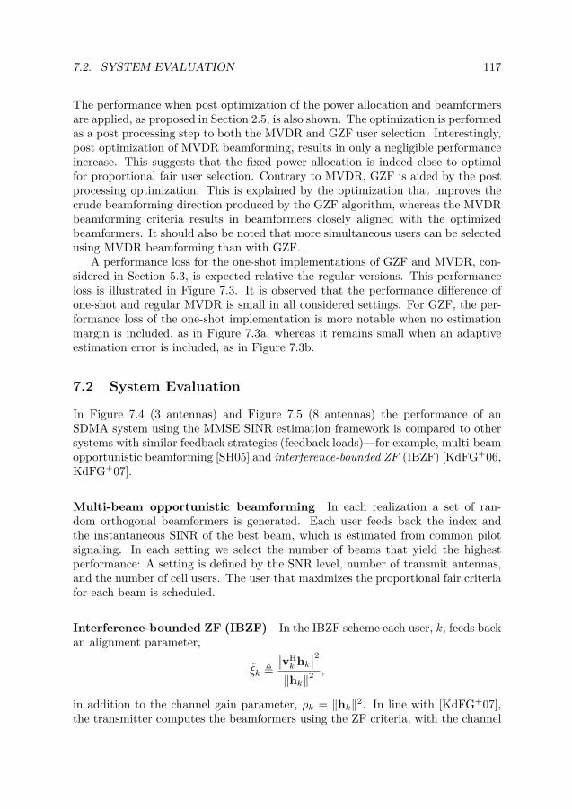
7.2. SYSTEM EVALUATION 117
The performance when post optimization of the power allocation and beamformersare applied, as proposed in Section 2.5, is also shown. The optimization is performedas a post processing step to both the MVDR and GZF user selection. Interestingly,post optimization of MVDR beamforming, results in only a negligible performanceincrease. This suggests that the fixed power allocation is indeed close to optimalfor proportional fair user selection. Contrary to MVDR, GZF is aided by the postprocessing optimization. This is explained by the optimization that improves thecrude beamforming direction produced by the GZF algorithm, whereas the MVDRbeamforming criteria results in beamformers closely aligned with the optimizedbeamformers. It should also be noted that more simultaneous users can be selectedusing MVDR beamforming than with GZF.
A performance loss for the one-shot implementations of GZF and MVDR, con-sidered in Section 5.3, is expected relative the regular versions. This performanceloss is illustrated in Figure 7.3. It is observed that the performance difference ofone-shot and regular MVDR is small in all considered settings. For GZF, the per-formance loss of the one-shot implementation is more notable when no estimationmargin is included, as in Figure 7.3a, whereas it remains small when an adaptiveestimation error is included, as in Figure 7.3b.
7.2 System Evaluation
In Figure 7.4 (3 antennas) and Figure 7.5 (8 antennas) the performance of anSDMA system using the MMSE SINR estimation framework is compared to othersystems with similar feedback strategies (feedback loads)—for example, multi-beamopportunistic beamforming [SH05] and interference-bounded ZF (IBZF) [KdFG+06,KdFG+07].
Multi-beam opportunistic beamforming In each realization a set of ran-dom orthogonal beamformers is generated. Each user feeds back the index andthe instantaneous SINR of the best beam, which is estimated from common pilotsignaling. In each setting we select the number of beams that yield the highestperformance: A setting is defined by the SNR level, number of transmit antennas,and the number of cell users. The user that maximizes the proportional fair criteriafor each beam is scheduled.
Interference-bounded ZF (IBZF) In the IBZF scheme each user, k, feeds backan alignment parameter,
ξk �∣∣vHk hk
∣∣2‖hk‖2
,
in addition to the channel gain parameter, ρk = ‖hk‖2. In line with [KdFG+07],the transmitter computes the beamformers using the ZF criteria, with the channel

118 CHAPTER 7. PERFORMANCE EVALUATION
GZF GZF one-shot MVDR MVDR one-shot
8 10 12 14 16 18 20 22 24 260
0.2
0.4
0.6
0.8
1
Cell throughput [bits/s/Hz]
4A
nten
nas
(a) No Estimation Error Margin
8 10 12 14 16 18 20 22 24 260
0.2
0.4
0.6
0.8
1
Cell throughput [bits/s/Hz]
4A
nten
nas
(b) Adaptive Estimation Error Margin
Figure 7.3: Evaluation of the one-shot implementations of GZF and MVDR. TheSNR is 10 dB and there are 20 users in the cell. The CDF of the cell throughputis shown for 4 and 8 antennas (increasing performance).

7.2. SYSTEM EVALUATION 119
estimates,hk =
√ξ‖hk‖vk.
Using the alignment, a lower bound on the instantaneous SINR of each user iscomputed [KdFG+07] and used for the rate adaptation. The greedy user selectionof Table 4.1 was used, which is similar to the greedy user-selection algorithm con-sidered in [KdFG+07]. The user-selection algorithms differ in that incompatibleusers are eliminated and a proportional fair criteria is used herein contrary to thesum-rate criteria in [KdFG+07].
MVDR beamforming with MMSE SINR estimation framework The per-formance of the MMSE SINR estimation framework is illustrated using user selec-tion with MVDR beamforming. An adaptive estimation error margin is appended,because the other compared schemes have, in theory, zero outage probability. Nopost optimization of the beamformers is performed.
It is observed in Figure 7.4 and Figure 7.5 that opportunistic beamforming isthe overall weakest performer. IBZF is able only to marginally outperform theproposed MMSE SINR estimation framework with MVDR beamforming, for thescenario with low SNR, few transmit antennas, and a handful of cell users, seeFigure 7.4a. Note however that IBZF requires the additional feedback of ξk, andthat the proposed MVDR beamforming, in most cases, significantly outperformsIBZF. The performance gain of MVDR beamforming is particularly significant insettings with high SNR and many transmit antennas.
We also take a look at the throughput of the individual users of the sys-tems. Figure 7.6 (3 antennas) and Figure 7.7 (8 antennas) show the CDFs ofthe user throughput that is achieved by opportunistic beamforming, IBZF, andMVDR beamforming with CGI feedback. We see that, with 20 users in the cell,the MVDR scheme outperforms the other schemes over the entire range. Thus,the performance advantage does not come at the expense of compromised fairnessamong the users. However, the improved suppression of co-channel interference,achieved with MVDR beamforming, benefits high performing users proportionallymore than it benefits the average user. This behavior is seen in Figure 7.7,where the performance gain of MVDR beamforming is significantly larger for highperformance users compared to the average user.
The performance of the MMSE SINR estimation framework does however de-pend on how correlated the channel is. The correlation decreases when the angularspread increases. The performance for different angular spreads is illustrated inFigure 7.8a. It is observed that the MMSE SINR estimation framework maintainsits performance advantage over the compared schemes for angular spreads as largeas σθ = 20 degrees. In Figure 7.8b the average cell throughput is illustrated fordifferent Ricean K-factors, K �
∥∥hk∥∥2 /Tr {Rk}. With Ricean fading the perfor-
mance advantage for the proposed framework is maintained, and for largeK-factorsthe throughput of the MVDR algorithm approaches that of ZF with perfect CSI.

120 CHAPTER 7. PERFORMANCE EVALUATION
Opp. Beamf. IB ZF MVDR, MMSE framework
1.5 2 2.5 3 3.5 4 4.5 5 5.5 60
0.2
0.4
0.6
0.8
1
Cell throughput [bits/s/Hz]
(a) The CDF of the cell throughput with SNR = 0 dB and 3 antennas
4 5 6 7 8 9 100
0.2
0.4
0.6
0.8
1
Cell throughput [bits/s/Hz]
(b) The CDF of the cell throughput with SNR = 10 dB and 3 antennas
Figure 7.4: System comparison of multi-beam opportunistic beamforming, interfer-ence bounded ZF and the proposed virtual-uplink MVDR beamforming, combinedwith the MMSE SINR estimation framework. The performance is given for 5 cellusers (dash-dotted) and 40 cell users (solid).

7.2. SYSTEM EVALUATION 121
Opp. Beamf. IB ZF MVDR, MMSE framework
2 4 6 8 10 120
0.2
0.4
0.6
0.8
1
Cell throughput [bits/s/Hz]
(a) The CDF of the cell throughput with SNR = 0 dB and 8 antennas
5 10 15 200
0.2
0.4
0.6
0.8
1
Cell throughput [bits/s/Hz]
(b) The CDF of the cell throughput with SNR = 10 dB and 8 antennas
Figure 7.5: System comparison of multi-beam opportunistic beamforming, interfer-ence bounded ZF and the proposed virtual-uplink MVDR beamforming, combinedwith the MMSE SINR estimation framework. The performance is given for 5 cellusers (dash-dotted) and 40 cell users (solid).

122 CHAPTER 7. PERFORMANCE EVALUATION
Opp. Beamf. IB ZF MVDR, MMSE framework
0 0.1 0.2 0.3 0.4 0.5 0.6 0.70
0.2
0.4
0.6
0.8
1
User throughput [bits/s/Hz]
(a) The CDF of the user throughput with SNR = 0 dB, 20 users, and 3 antennas
0 0.1 0.2 0.3 0.4 0.5 0.6 0.70
0.2
0.4
0.6
0.8
1
User throughput [bits/s/Hz]
(b) The CDF of the user throughput with SNR = 10 dB, 20 users, and 3 antennas
Figure 7.6: Comparison (3 antennas) of the user throughput achieved by multi-beam opportunistic beamforming, interference bounded ZF and the proposedvirtual-uplink MVDR beamforming that is combined with the MMSE SINR es-timation framework.
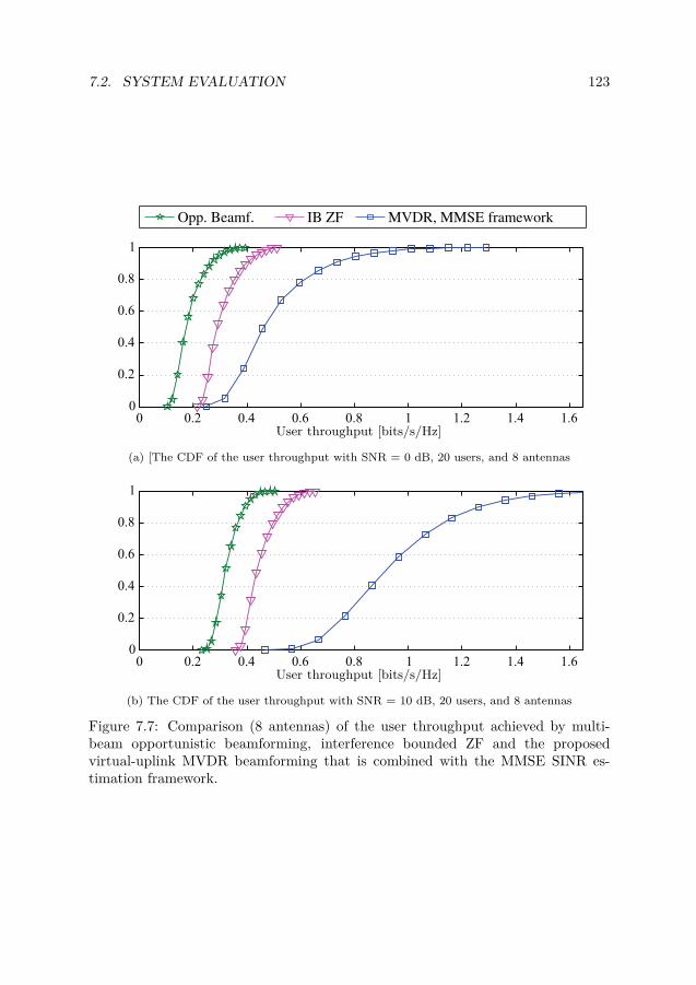
7.2. SYSTEM EVALUATION 123
Opp. Beamf. IB ZF MVDR, MMSE framework
0 0.2 0.4 0.6 0.8 1 1.2 1.4 1.60
0.2
0.4
0.6
0.8
1
User throughput [bits/s/Hz]
(a) [The CDF of the user throughput with SNR = 0 dB, 20 users, and 8 antennas
0 0.2 0.4 0.6 0.8 1 1.2 1.4 1.60
0.2
0.4
0.6
0.8
1
User throughput [bits/s/Hz]
(b) The CDF of the user throughput with SNR = 10 dB, 20 users, and 8 antennas
Figure 7.7: Comparison (8 antennas) of the user throughput achieved by multi-beam opportunistic beamforming, interference bounded ZF and the proposedvirtual-uplink MVDR beamforming that is combined with the MMSE SINR es-timation framework.

124 CHAPTER 7. PERFORMANCE EVALUATION
ZF, Full CSI MVDR GZF IBZF Opp. BF
0 5 10 15 20 250
5
10
15
20
25
Cel
lthr
ough
put
[bits
/s/H
z]
Angular spread [degrees]
(a) Average cell throughput for different angular spreads.
0 2 4 6 8 10 12 14 160
5
10
15
20
25
Cel
lthr
ough
put
[bits
/s/H
z]
Ricean K-factor(b) Average cell throughput for different Ricean K-factors.
Figure 7.8: Evaluation of the average cell throughput of the proposed MVDRscheme for parameters affecting the channel distribution (angular spread, σθ, andRicean K-factor). An adaptive estimation error margin is used and the systemparameters are set as, SNR = 10dB, 6 transmit antennas, and 20 cell users.

7.3. FINITE RATE FEEDBACK 125
7.3 Finite Rate Feedback
In the preceding we assumed that the user terminals could feed back ρk with infiniteresolution, which would require infinite feedback capacity. In practice ρk must bequantized using only a few bits, which results in a performance loss. Next, wepropose a quantization scheme and evaluate the performance when the feedback islimited to b bits per user.
We quantize ρk into ρk, which belongs to a finite reproduction alphabet:
ρk ∈ Rk = {0, ρ(1)k , ρ
(2)k , . . . , ρ
(2b−1)k }, where ρ(m1)
k < ρ(m2)k ∀m1 < m2.
The users feed back the quantized level—or rather its index—and the transmitteruses ρ as if it was the actual (infinite resolution) channel gain. Because we want toavoid outages at the transmitter, the quantization level is chosen as
ρk =Q(ρk) � max{ ρ | ρ ∈ Rk, ρ ≤ ρk};that is, we select the reproduction point of each quantization interval as the mini-mum value of the interval.
We propose an heuristic approach for choosing the quantization levels ρ(m)k and
do not claim any kind of optimality. However, we show that also with simpleheuristic methods, the performance loss of finite rate feedback is limited. Theheuristic approach takes advantage of the following observations:
1. The resource scheduler is primarily interested in large realizations of ρk. Userswith small realizations feed back ρk = 0 and are not candidates for scheduling.
2. There should be sufficiently many users with ρk ≥ 0, so that a spatiallycompatible set of users can be scheduled.
3. The quantization levels should be different for each user and adapt to thestatistics of ρ as well as the total number of users in the cell.
The choice of ρk,min = ρ(1)k is directly related to the two first points. We set the
design goal that on the average there should be
nC = nC(b,K, nT ),
candidates in the resource allocation—that is, on the average nC users should feedback ρk > 0. The parameter, nC , is a design parameter that should be increasedwith increasing nT ; with more antennas, more users are allocated. The numberof users with ρk > 0 has a binomial distribution, B(K,α), where K is the totalnumber of users, and α is the probability that ρk > 0. Thus, the expected numberof candidates is Kα, which translates into the following design criterion for ρk,min:The minimum quantization level, ρk,min, is solved from
Pr {ρ > ρk,min} = α � min{
(1− 2−b), nCK
}. (7.1)

126 CHAPTER 7. PERFORMANCE EVALUATION
0
0.5
1
(1− α)
ΔΔΔ
ρkρ(1)k ρ
(2)k ρ
(3)k
Q(ρk) : 0 ρ(1)k ρ
(2)k ρ
(3)k
Cumulative Distribution Function of ρk
Figure 7.9: Illustration of the finite rate quantization scheme.
To handle the case K < nC , for which the design goal obviously cannot be met, theprobability, α, is upper bounded to (1 − 2−b). The remaining quantization levels,ρ
(2)k , . . . , ρ
(2b−1)k , are chosen such that they are equally probable:
Pr{ρ > ρ
(m)k
}= α(1− m− 1
2b − 1), m = 1, . . . , 2b − 1.
The quantization scheme is illustrated in Figure 7.9.To maximize the performance, nC should be adapted with b, K and the SNR:
Simulations indicate that the throughput maximizing nC is an increasing functionof b and K. However, for simplicity we set nC as
nC ={nT2 , b = 1,nT , otherwise,
which gives reasonable performance in the considered scenarios. The transmitteruses the quantized CGI, as if it was the actual channel gain (i.e., as if ρk = ρk).An adaptive estimation error margin is also applied where, as in the previous sim-ulations,1 α = 2.
The simulated performance of the proposed finite rate scheme, with MVDRbeamforming and greedy user selection, is shown in Figure 7.10 and Figure 7.11
1 The quantization scheme has an inherent robustness to estimation errors, because ρk ≤ρ. The outage probability is therefore smaller with quantized feedback than it is in the othersimulations; for example, with 1 bit or 2 bits feedback, the outage probability does not exceed 1.6percent in any of the simulations.

7.3. FINITE RATE FEEDBACK 127
b = 1 b = 2 b = 3 b = 4 b =∞
0 2 4 6 8 10 120
0.2
0.4
0.6
0.8
1
Cell throughput [bits/s/Hz]
4A
nten
nas
(a) The CDF of the cell throughput with SNR = 0 dB and 10 users
0 2 4 6 8 10 120
0.2
0.4
0.6
0.8
1
Cell throughput [bits/s/Hz]
4A
nten
nas
(b) The CDF of the cell throughput with SNR = 0 dB and 40 users
Figure 7.10: Performance evaluation (SNR=0 dB) of MVDR beamforming withfinite rate feedback and greedy user selection. For comparison, also the performanceof MVDR, with ρk fully known, is given (marked b = ∞). The CDF of the cellthroughput, as realized over the random scenarios, is shown for 4 and 8 antennas(increasing performance).
for the SNR values 0 dB and 10 dB, respectively. With 2 bits of feedback, thereis approximately a 1 bits/s/Hz performance loss in the 4 antenna case, and a 2bits/s/Hz performance loss for 8 antennas. Also, with 1 bit of feedback, the perfor-mance loss is limited, and the finite rate scheme achieves a significant fraction of theperformance achieved with perfectly known ρk. This is explained by the multiuserdiversity, which is utilized by the proposed finite rate scheme. The performancegap between fully known ρk and b = 4, is to a large extent due to the choice of
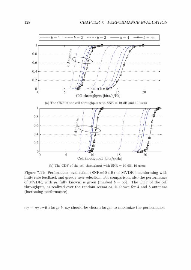
128 CHAPTER 7. PERFORMANCE EVALUATION
b = 1 b = 2 b = 3 b = 4 b =∞
0 5 10 15 200
0.2
0.4
0.6
0.8
1
Cell throughput [bits/s/Hz]
4A
nten
nas
(a) The CDF of the cell throughput with SNR = 10 dB and 10 users
0 5 10 15 200
0.2
0.4
0.6
0.8
1
Cell throughput [bits/s/Hz]
4A
nten
nas
(b) The CDF of the cell throughput with SNR = 10 dB, 10 users
Figure 7.11: Performance evaluation (SNR=10 dB) of MVDR beamforming withfinite rate feedback and greedy user selection. For comparison, also the performanceof MVDR, with ρk fully known, is given (marked b = ∞). The CDF of the cellthroughput, as realized over the random scenarios, is shown for 4 and 8 antennas(increasing performance).
nC = nT ; with large b, nC should be chosen larger to maximize the performance.

Chapter 8
Generalization of the CGIParameter
In this chapter, we generalize the results of Chapter 6 and consider the feedback ofa weighted norm of the channel vector,
ζk � ‖Akhk‖2 , (8.1)
where the matrix Ak ∈ Cna,k×nT can be chosen arbitrarily. Hence, ρk = ‖hk‖2 isthe special case when Ak is the identity matrix. We will in general consider Akto be a matrix with more columns than rows (i.e., na,k ≤ nT ), even though this isnot a strict requirement of the framework. We show how to express the conditionalmoments of hk for a given ζk, in terms of quantities that can be efficiently computedusing the framework in Chapter 6.
By introducing the weighted norm, additional degrees of freedom are madeavailable in the system design. An application of particular interest is to decreasethe overhead by exciting only a subset of the antennas during the pilot signaling. Toaccurately estimate hk ∈ CnT or ‖hk‖2 at the receivers, all nT complex dimensionsof the propagation channel must be excited, which requires a pilot signaling intervalof at least nT symbols due to orthogonality constraints. In multi-cell systems theoverhead is even more severe because pilot sequences of neighboring cells are oftenrequired to be orthogonal. For large nT this, otherwise significant, overhead canbe remedied by exciting only na � nT antennas. By letting each row of Ak = Ahave a single non-zero element (corresponding to an active antenna element), thereceivers can estimate ζk even though the remaining elements remain passive. Thetransmitter can next combine ζk with the CDI and use the full antenna array forthe data transmission. The performance evaluation in Section 8.2 shows that it issufficient to excite just a few antennas to achieve a negligible performance loss overusing ρk = ‖hk‖2.
Using the generalized framework for weighted norms, we also show how to com-pute good approximations of the conditional moments—at a significantly reduced
129
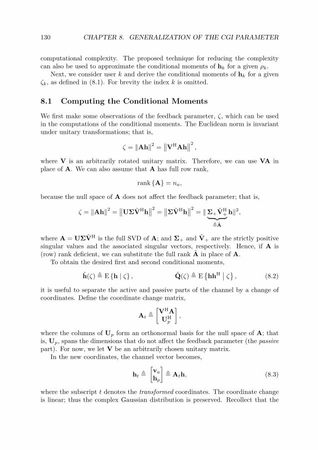
130 CHAPTER 8. GENERALIZATION OF THE CGI PARAMETER
computational complexity. The proposed technique for reducing the complexitycan also be used to approximate the conditional moments of hk for a given ρk.
Next, we consider user k and derive the conditional moments of hk for a givenζk, as defined in (8.1). For brevity the index k is omitted.
8.1 Computing the Conditional Moments
We first make some observations of the feedback parameter, ζ, which can be usedin the computations of the conditional moments. The Euclidean norm is invariantunder unitary transformations; that is,
ζ = ‖Ah‖2 =∥∥VHAh
∥∥2,
where V is an arbitrarily rotated unitary matrix. Therefore, we can use VA inplace of A. We can also assume that A has full row rank,
rank {A} = na,
because the null space of A does not affect the feedback parameter; that is,
ζ = ‖Ah‖2 =∥∥UΣVHh
∥∥2 =∥∥ΣVHh
∥∥2 = ‖Σ+VH+︸ ︷︷ ︸
�A
h‖2,
where A = UΣVH is the full SVD of A; and Σ+ and V+ are the strictly positivesingular values and the associated singular vectors, respectively. Hence, if A is(row) rank deficient, we can substitute the full rank A in place of A.
To obtain the desired first and second conditional moments,
h(ζ) � E {h | ζ} , Q(ζ) � E{
hhH ∣∣ ζ} , (8.2)
it is useful to separate the active and passive parts of the channel by a change ofcoordinates. Define the coordinate change matrix,
At �[VHAUHp
],
where the columns of Up form an orthonormal basis for the null space of A; thatis, Up, spans the dimensions that do not affect the feedback parameter (the passivepart). For now, we let V be an arbitrarily chosen unitary matrix.
In the new coordinates, the channel vector becomes,
ht �[vahp
]� Ath, (8.3)
where the subscript t denotes the transformed coordinates. The coordinate changeis linear; thus the complex Gaussian distribution is preserved. Recollect that the
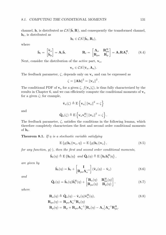
8.1. COMPUTING THE CONDITIONAL MOMENTS 131
channel, h, is distributed as CN (h,R), and consequently the transformed channel,ht, is distributed as
ht ∈ CN (ht,Rt),where
ht =[vahp
]= Ath, Rt =
[Λa RH
pa
Rpa Rp
]= AtRAH
t . (8.4)
Next, consider the distribution of the active part, va,
va ∈ CN (va,Λa).
The feedback parameter, ζ, depends only on va and can be expressed as
ζ = ‖Ah‖2 = ‖va‖2 .The conditional PDF of va for a given ζ, f(va|ζ), is thus fully characterized by theresults in Chapter 6, and we can efficiently compute the conditional moments of vafor a given ζ; for example,
va(ζ) � E{
va∣∣ ‖va‖2 = ζ
}and
Qa(ζ) � E{
vavHa
∣∣ ‖va‖2 = ζ}.
The feedback parameter, ζ, satisfies the conditions in the following lemma, whichtherefore completely characterizes the first and second order conditional momentsof ht.
Theorem 8.1. If η is a stochastic variable satisfying
E {g(ht)|va, η} = E {g(ht)|va} , (8.5)
for any function, g(·), then the first and second order conditional moments,
ht(η) � E {ht|η} and Qt(η) � E{
hthHt |η
},
are given by
ht(η) = ht +[
IRpaΛ−1
a
](va(η)− va) (8.6)
andQt(η) = ht(η)hH
t (η) +[
Ra(η) RHpa(η)
Rpa(η) Rp(η)
], (8.7)
where
Ra(η) � Qa(η)− va(η)vHa (η), (8.8)
Rpa(η) = RpaΛ−1a Ra(η)
Rp(η) = Rp + RpaΛ−1a
[Ra(η)−Λa
]Λ−1a RH
pa.

132 CHAPTER 8. GENERALIZATION OF THE CGI PARAMETER
Proof. The proof is given in Appendix 8.A.
Using Theorem 8.1 we can compute the transformed conditional moments, ht(ζ)and Qt(ζ), and the sought conditional moments are obtained by transforming backto the original coordinates as
h(ζ) = A−1t ht(ζ),
Q(ζ) = A−1t Qt(ζ)A−H
t .
Note that At is invertible, because A can be assumed full rank.Also the fourth order moment, E
{ ∣∣wHh∣∣4 ∣∣ ζ}, can be computed from the con-
ditional moments of va. To achieve this, we introduce the transformed beamformer,wt:
wt �[wawp
]� A−H
t w,
so that wHh = wHt ht. The following corollary characterizes the forth order condi-
tional moments:
Corollary 8.2. For η satisfying (8.5), the conditional fourth order moment is givenby,
E{∣∣wHh
∣∣4 ∣∣η} = 2(σ2 +∣∣hp∣∣2 +m2)2 +m4 −
∣∣hp∣∣4 − 2m22
+ 2�{
2h∗p[( ∣∣hp∣∣2 + 2σ2)m1 +m3
]+ (h∗p)2m2T
},
where
σ2 = wHp
(Rp −RpaΛ−1
a RHpa
)wp,
hp = wHp (hp −RpaΛ−1
a va),
and the remaining parameters are expressed in
wa � wa + Λ−1a RH
pawp,
as
m1 = wHa va(η), m2 = wH
a Qa(η)wa,
m2T = wHa E
{vavTa |η
}w∗a, m3 = wH
a E{[
vTa ⊗ vavH
a
] ∣∣∣η} vec(wawHa )
andm4 =
(vec(wawH
a ))HE
{[v∗avT
a ⊗ vavHa
] ∣∣∣η} vec(wawHa ).
Proof. The proof is given in Appendix 8.B.

8.2. PERFORMANCE EVALUATION OF PILOT SIGNALING ONSELECTED ANTENNAS 133
For zero-mean channels, the expression for the fourth order moment is simplified.The fourth order moments of the Rayleigh fading channel are given by the followinglemma:
Corollary 8.3. For Rayleigh fading channels, the fourth order conditional momentof vt for a given ζ, is given by
M4t(ζ) � E{
v∗tvTt ⊗ vtvH
t | ζ}
= 2QTt (ζ)⊗ Qt(ζ) + Z
[M4a(ζ)− 2QT
a (ζ)⊗Qa(ζ)]ZH,
where
M4a � E{
v∗avTa ⊗ vavH
a | ζ},
Z =[
IRpaΛ−1
a
]∗⊗[
IRpaΛ−1
a
]∈ CnTnT×nana ,
and the fourth order conditional moment of wHh is given by,
E{∣∣wHh
∣∣4 | ζ} =(vec(wtwH
t ))H M4t(ζ) vec(wtwH
t ). (8.9)
Proof. The proof is given in Appendix 8.C.
In the preceding we have not assumed that the covariance matrix of va,
Λa � VHARAHV,
is diagonal, even though the notation suggests so. There are however good reasonsto ensure that Λa is diagonal: it is easier to invert the matrix, and the results ofChapter 6 are better suited for independent elements in va. Fortunately, we canuse the flexibility introduced by V to make Λa diagonal; that is, we define V as
V � [v1,v2, . . . ,vna ], (8.10)
where vi are the eigenvectors of ARAH. With this definition of V, the covari-ance matrix, Λa, is diagonal. Using the white coordinates, E
{|wHh|4 | ζ} can becomputed using Corollary 8.2 and the results in Chapter 6.
8.2 Performance Evaluation of Pilot Signaling on SelectedAntennas
As was discussed above, feeding back the full channel norm, ‖hk‖2, may requiresignificant common pilot signaling because all dimensions of the channel must beexcited. The amount of overhead can therefore be significantly reduced by excitingonly a small subset of the antennas and feed back the parameter, ζk =
∑i∈A |[hk]i|2,
where A is the set of active antennas. The transmitter next combines the feedback

134 CHAPTER 8. GENERALIZATION OF THE CGI PARAMETER
12 14 16 18 200
0.2
0.4
0.6
0.8
1
1 Antenna
2 Antennas
4 Antennas
8 Antennas
Cell throughput [bits/s/Hz]
Figure 8.1: Performance of the MMSE SINR estimation framework with MVDRbeamforming, when only a subset of the antennas are active in the pilot signaling.The figure shows the CDF of the average cell throughput for a MVDR system withSNR = 10dB, 8 transmit antennas, 20 users, and adaptive estimation error margin.
information with the statistics of the full channel vector, and uses the full antennaarray in the data transmission.
This scheme is evaluated in Figure 8.1, where a system with an 8 element UCAis considered, but only one, two or four elements are active in the plot signaling.The same simulation setup as in Chapter 7 is used and the active pilot antennas aredistributed evenly over the UCA. As observed in the figure, the performance lossof only using one pilot antenna is significant, whereas two pilot antennas resultsonly in a small performance loss over four and eight pilot antennas, where theperformance difference is negligible.
8.3 Approximation for Reduced Complexity
Even though the conditional moments of va ∈ Cna can be efficiently computed usingthe algorithms developed in Chapter 6, the computational complexity grows rapidlywith the dimension of va. The complexity grows particularly fast for Ricean fadingchannels: The complexity of computing the fourth order moment, E
{|wHa va|4
∣∣ζ},grows proportional to n5
a (with precomputed parameters). Thus, there is much togain by reducing the dimensionality of the problem; next, we propose an approxi-mation to achieve such a reduction.
We consider the generalized feedback parameter,
ζ = ‖Ah‖2.
In the following we show that in the computations, the transmitter can instead

8.3. APPROXIMATION FOR REDUCED COMPLEXITY 135
consider an alternative feedback parameter,
ζD = ‖ADh‖2
where AD ∈ Cna×nT and na � na; that is, the dimensionality is significantlydecreased. We show that ζD can be accurately estimated from ζ—and vice versa;the gains, ζD, and ζ, thus carry almost the same information about the channelrealization. To reduce the computational burden, the transmitter can use AD andan estimate of ζD, in place of A and ζ. If na is not set too small, the loss in accuracyintroduced by the approximation is negligible, at least for large realizations of ζ.Note that this approach is also applicable for ζ = ‖h‖2, as considered in Chapter 6,where A is the identity matrix.
To obtain this approximation we take the approach of dividing ζ into a dynamicpart and a “static” part,
ζ = ζD + ζS , (8.11)
where ζS is static in the sense that its variations are much smaller than those ofζD. To separate the static and dynamic part we change coordinates, as in (8.4), to
ht =[vahp
]=[VHAUHp
]h.
We also let V be defined as in (8.10), so that the elements of va are independent;that is,
va ∈ CN (va,Λa),
where Λa is diagonal. Moreover, we let the diagonal elements of Λa be ordereddecreasingly, and partition them into the large eigenvalues, ΛL ∈ Cna×na , and thesmall eigenvalues, ΛS . In summary,
ARAH = VΛaVH = [VLVS ][ΛL 00 ΛS
][VLVS ]H.
The elements in va are thus independent and have decreasing variance; we partitionva as
va =[vDvS
]=[(VL)H
(VS)H
]Ah �
[ADAS
]h,
where vD represents the elements with largest variance, and vS the “static” ele-ments with smallest variance. Consequently, ζD and ζS are defined as
ζD � ‖vD‖2 = ‖ADh‖2 ,ζS � ‖vS‖2 = ‖ASh‖2 ,
which satisfies (8.11), because
ζ =∥∥[VLVS ]HAh
∥∥2 =∥∥VHLAh
∥∥2 +∥∥VHSAh
∥∥2 = ζD + ζS .

136 CHAPTER 8. GENERALIZATION OF THE CGI PARAMETER
We can estimate ζS as
ζS = ‖vS‖2 ≈ E{‖vS‖2
}= ‖vS‖2 + Tr {ΛS} =
∥∥VHSAh
∥∥2 + Tr {ΛS} ,
where the approximation follows by noting that the variations in ‖vS‖2 are smallrelative ζ—in particular for large values of ζ, see Chapter 6.
We thus have the relation,
ζD ≈ ζ −∥∥VHSAh
∥∥2 − Tr {ΛS} .Note that, for very small realizations of ζ, this is a poor approximation:
limζ→0ζ − ∥∥VH
SAh∥∥2 − Tr {ΛS} = −∥∥VH
SAh∥∥2 − Tr {ΛS} < 0,
whereas ζD is a norm, and thus positive. In practice these small realizations of ζare irrelevant, and we can use the estimate
ζD = max{0, ζ − ∥∥VHSAh
∥∥2 − Tr {ΛS}}for computational robustness.
To demonstrate the accuracy of the proposed approximation, we consider aRayleigh fading channel with the statistics that was used in the simulations inChapter 7; that is, the transmitter has an 8 antenna UCA with 1 wavelengthdiameter, and the scattering is modeled as complex Gaussian distributed with an-gular spread 10 degrees [ZO94b]. The transmitter knows the square channel norm,ρ = ‖h‖2. We let the dominating part be the two dominating eigenmodes; that is,na = 2.
To measure the deviation of the approximated MMSE estimates, QζD (ζD), fromthe true MMSE estimate, Qρ(ρ), we look at the norm of their difference; that is,the deviation is ∥∥∥Qρ(ρ)− QζD (ζD)
∥∥∥ ,where the norm refers to the spectral norm (i.e., the maximum singular value ofthe matrix). The deviation depends on the azimuth angle (i.e., the direction of theuser) and we therefore average the deviation over all azimuth angles; that is, weconsider the relative mean deviation measure,
E{∥∥∥Qρ(ρ)− QζD (ζD)
∥∥∥}E{∥∥∥Qρ(ρ)
∥∥∥} ,
where the expectation is with respect to the azimuth angle. Figure 8.3 shows thisrelative mean approximation error as a function of ρ. We observe from the figurethat the relative error is significant for small values of ρ, but negligible for ρ largerthan half of its expected value.

8.A. PROOF OF THEOREM 8.1 137
0
0.2
0.4
0.6
0.8
1
ρE{ρ}R
el.
Mea
nA
ppro
x.Er
ror
Figure 8.2: Shows the relative mean approximation error in an 8 antenna systemwith angular spread 10 degrees, using na = 2. The expected value of ρ is indicatedin the figure, and determines the scaling.
8.A Proof of Theorem 8.1
Proof. Let Mx(y) denote a conditional moment (of arbitrary order) of x for a giveny. The moment, Mht(η), can be expressed in terms of Mht(va) as
Mht(η) = Eva {Mht(va)|η} . (8.12)
This follows from the expansion,
Mht(η) � Eht {Mht(ht)|η} = Eva{
Ehp {Mht(ht)|va, η} |η},
and by noting that the conditioning on η in the inner expectation can be droppedbecause ht, by assumption, depends only on η through va, which is fully determinedin this expectation.
Hence, we start by evaluating Mht(va) and next proceed with the outer ex-pectation. For a given va the stochastic behavior of ht is fully described by thedistribution of hp|a, which is interpreted as hp for a given va. Also hp|a is complexGaussian [KSH00] and distributed as
hp|a ∈CN (hp|a,Rp|a),{
Rp|a � Rp −RpaR−1a RH
pa,
hp|a � hp + RpaR−1a (va − va),
(8.13)
where Rp|a is the Schur complement of Ra in (8.4). Note that hp|a = hp|a(va),whereas the conditional covariance, Rp|a, is unaffected by the actual realization ofva. It follows that the first order conditional moment or ht for a given va is givenby
ht(va) � E {ht|va} =[
vahp|a
]= ht +
[I
RpaΛ−1a
](va − va),

138 CHAPTER 8. GENERALIZATION OF THE CGI PARAMETER
from which ht(η) = E {ht|η} is obtained as in (8.6) by applying the outer expecta-tion described in (8.12).
To obtain the second order conditional moment, Qt(η), we start with the ex-pansion
E{
ht(va)hHt (va)|η
}= ht(η)hH
t (η) + E{[
ht(va)− ht(η)][
ht(va)− ht(η)]H∣∣∣η}
= ht(η)hHt (η) +
[I
RpaΛ−1a
]Ra(η)
[I
RpaΛ−1a
]H
, (8.14)
where Ra(η) is defined in (8.8). From (8.13) it follows that the conditional moment,E{
hthHt |va
}, is given by
E{
hthHt |va
}= ht(va)hH
t (va) +[0 00 Rp|a
]which, if combined with (8.12) and (8.14), yields the expression for Qt(η) in (8.7).
8.B Proof of Corollary 8.2
Proof. Define the stochastic variableh � wHh = wH
t ht = wHa va + wH
p hp.It follows from (8.13), that for a given va, the scalar, h, is complex Gaussiandistributed as
h ∈ CN (h, σ2),{σ2 = wH
p
(Rp −RpaΛ−1
a RHpa
)wp,
h = wHa va + wH
p hp|a.
Note that σ2 is a constant, independent of va. The mean component, h, doeshowever depend on va, but by writing it as
h = hp + va,we can isolate the dependence to va, by the following definitions:
hp � wHp (hp −RpaΛ−1
a ha),va � wH
a va,wa � wa + Λ−1
a RHpawp.
The fourth order moment, for a given va, is obtained as [Kay93],
E{|h|4 ∣∣va} = 2σ4 +
∣∣h∣∣4 + 4σ2 ∣∣h∣∣2= 2σ4 +
∣∣hp∣∣4 + 4σ2 ∣∣hp∣∣2 + |va|4 + 4(∣∣hp∣∣2 + σ2) |va|2
+ 2�{
2h∗p[( ∣∣hp∣∣2 + 2σ2)va + |va|2 va
]+ (h∗p)2v2a
}, (8.15)

8.C. PROOF OF COROLLARY 8.3 139
where the identity
|a+ b|4 = |a|4 + |b|4 + 4 |a|2 |b|2 + 2�{
2 |a|2 ab∗ + 2 |b|2 ba∗ + a2b∗2}, ∀a, b ∈ C,
was used to expand ∣∣h∣∣4 =∣∣va + hp
∣∣4 .In (8.15), the only parameter depending on va is va. By averaging over va thesought fourth order moment is obtained as
E{∣∣wHh
∣∣4 |ζ} = Eva
{E{|h|4 ∣∣va} |ζ}
= 2σ4 +∣∣hp∣∣4 + 4σ2 ∣∣hp∣∣2 +m4 + 4(
∣∣hp∣∣2 + σ2)m2
+ 2�{
2h∗p[( ∣∣hp∣∣2 + 2σ2)m1 +m3
]+ (h∗p)2m2T
}, (8.16)
where
m1 � E {va|η} ,m2 � E
{|va|2
∣∣η} ,m2T � E
{v2a∣∣η} ,
m3 � E{|va|2 va
∣∣∣ η} ,m4 � E
{|va|4 |η
}.
The theorem follows by completing the squares in (8.16) and by expanding theconditional moments of va = wH
a va, using (B.5) and (B.6) in Appendix B.
8.C Proof of Corollary 8.3
Proof. In Rayleigh fading channels, the expression for E{|wHh|4 | ζ} in Corol-lary 8.2, simplifies to
E{∣∣wHh
∣∣4 | ζ} = 2(σ2 +m2)2 +m4 − 2m22,
because the remaining parameters are zero. We begin by rewriting E{∣∣wHh
∣∣4 | ζ}as a quadratic form in vec(wtwH
t ), and then identifies the expressions in the corol-lary.
First consider σ2 +m2, which is given by
σ2 +m2 = wHp
(Rp −RpaΛ−1
a RHpa
)wp + wH
a Qa(ζ)wa
= wHt
([0 00 Rpa −RpaΛ−1
a RHpa
]+[
IRpaΛ−1
a
]Qa(ζ)
[I
RpaΛ−1a
]H)
wt
= wHt Qt(ζ)wt,

140 CHAPTER 8. GENERALIZATION OF THE CGI PARAMETER
where the last identity follows from (8.7) in Theorem 8.1, because ht(ζ) and va(ζ)are zero for Rayleigh fading channels. Using this expression for σ2 +m2, we canwrite (σ2 +m2)2 as
(σ2 +m2)2 = Tr{
wtwHt Qa(ζ)wtwH
t Qa(ζ)}
=(vec(wtwH
t ))H(QT
t (ζ)⊗ Qt(ζ))vec(wtwH
t ),
where the last identity follows from (B.4) in Appendix B.It remains to express m4 − 2m2
2 in terms of vec(wtwHt ). We can write m2
2 as aquadratic form in vec(wawH
a ) as
m22 = Tr
{wawH
a Qa(ζ)wawHa Qa(ζ)
}=
(vec(wawH
a ))H(QT
a (ζ)⊗ Qa(ζ))vec(wawH
a ),
where we again apply (B.4) in Appendix B. Also m4 is, by definition, a quadraticform in vec(wawH
a ), and by noting that
vec(wawHa ) = vec(
[I
RpaΛ−1a
]H
wtwHt
[I
RpaΛ−1a
]) = ZHvec(wtwH
t ),
where the last identity follows from (B.3) in Appendix B, we obtain the followingexpression
E{∣∣wHh
∣∣4 | ζ} =(vec(wtwH
t ))HM4t(ζ)vec(wtwH
t )
=(vec(wtwH
t ))H(
2QTt (ζ)⊗ Qt(ζ)+Z
[M4a(ζ)–2QT
a (ζ)⊗Qa(ζ)]ZH
)vec(wtwH
t ),
where the first equality follows from (B.6) in Appendix B, and the second equal-ity follows from the preceding discussion. The above expression holds for all w;therefore,
M4t(ζ) = 2QTt (ζ)⊗ Qt(ζ) + Z
[M4a(ζ)− 2QT
a (ζ)⊗Qa(ζ)]ZH,
and the corollary follows.
Chapter 9
Thesis Conclusions
Available algorithms for the downlink beamforming problems, have been general-ized to cope with additional indefinite shaping constraints. It was proven that therelaxed semidefinite formulation does solve the original beamforming problems op-timally. It was also shown how the more specialized and computationally efficientalgorithms presented in [SB04] may be generalized. By modifying only a subprob-lem in each iteration of the original algorithm, the optimization problem includingthe shaping constraints can be solved. The convergence to the optimal point re-mains, and an algorithmic solution to the constrained subproblem is presented.
Several applications for the proposed class of shaping constraints have also beendemonstrated. In particular, path diversity constraints in DS-CDMA systems wereformulated. The presented simulation results show how such constraints may im-prove the robustness of the link. Several interference limiting constraints were alsoproposed to suppress inter-cell interference in different scenarios.
An MMSE SINR tracking framework has been established, which is suitablefor resource allocation in best effort multi antenna, wide-area systems. The frame-work effectively combines slowly changing channel distribution information, as-sumed available at the transmitter, with partial instantaneous channel state infor-mation feedback. In particular the instantaneous feedback of a scalar channel gainparameter is considered. Efficient algorithms were developed for computing therequired MMSE estimates, as well as the resulting MSE, which enable an efficientsystem with adaptive SINR back off margins to achieve a target outage probability.Asymptotic results show that for strong channel norm realizations the channel isalmost fully determined, with a relative estimation error tending to zero. Hence, insystems with channel dependent scheduling where only users with strong channelsare scheduled, the scalar norm feedback provides similar performance as the casewith perfect CSI.
A greedy user selection scheme and several beamforming techniques, suitablefor the MMSE SINR tracking framework were proposed and evaluated. It wasdemonstrated that, in wide-area systems, it is sufficient to feed back a single scalar
141

142 CHAPTER 9. THESIS CONCLUSIONS
gain parameter from each user to achieve good performance for SDMA systems, ifthe channel distribution information is properly utilized. The proposed frameworkwas further shown to significantly outperform other techniques based on similarfeedback. Similar performance was also achieved when common pilot signaling isrestricted to only a small subset of the transmit antennas.

Appendix A
Nomenclature
In this appendix we summarize the notational convention of the thesis. First, weoverview the notation of more general nature. Next, the symbols and functions,more specific for this thesis, are listed. We conclude with a list of abbreviations.
A.1 Notation
The notation used in this thesis is summarized in this appendix. Plain letter, e.g. xand X, are used for scalars (complex or real). Boldface letters are used for vectors(lower case, e.g., x), and matrices (upper case, e.g., X). Sets are denoted with up-percase calligraphic letters (e.g., S). Boldface calligraphic letters (e.g., P) are usedfor optimization problems. No notational distinction is used for a random variableand its realization. Other notational conventions are summarized as follows:
R, C, Z, N The sets of real, complex, integer and natural numbers, re-spectively.
�{x}, �{x} The real and imaginary part of x, respectively.[x]i, [X]ij The ith element of a vector x, and the element in the ith
row and jth column of a matrix X, respectively.|a| The absolute value of a real or complex scalar.∠a The phase (argument) of a complex scalar (in radians).�a� The floor operator; that is, the largest integer less or equal
to a.|A| The cardinality of the set A; that is, the number of elements
in a finite set A.Am The Cartesian product, Am = A×A× · · · × A.A ∪ B The union of the sets A and B.
143

144 APPENDIX A. NOMENCLATURE
A \ B The relative complement of B in A; that is,
A \ B = {x|x ∈ A, x ∈ B}.
� Equal by definition.A � B A is greater than B in the sense that A − B is positive
semidefinite.A � B A is strictly greater than B in the sense that A − B is
positive definite.N (h,R) The (real valued) Gaussian distribution with mean h and
covariance matrix R.CN (h,R) The circular-symmetric complex Gaussian distribution with
mean h and covariance matrix R.E {x} The expected value of a stochastic random variable x.E {x|ϑ} The conditional expected value given ϑ.I The identity matrix.0 The zero vector or zero matrix.1 The vector (or matrix) of all ones.xT, XT The transpose of a vector, x, or a matrix, X.x∗, X∗ the conjugate of a vector, x, or a matrix, X.xH, XH The Hermitian transpose of a vector, x, or a matrix, X.X−1 The inverse of a matrix X.X† The Moore-Penrose pseudo inverse of X.‖x‖ The Euclidean norm of a vector x.⊗ The Kronecker matrix product.vec(X) The vector obtained by stacking the columns of X.Tr {X} The trace of matrix X (the sum of the diagonal elements).diag {x} The diagonal matrix with the elements of x on its diagonal.� The convolution operator.�© The circular convolution operator.DF {·}, DF−1 {·} The DFT and inverse DFT operators, respectively.L{·}, L−1 {·} The Laplace transform and inverse Laplace transform, re-
spectively.valP The globally optimal value of optimization problem P .x� An optimal point with respect to an optimization problem
parameterized by x.argP The set of globally optimal points of optimization problem
P .arg maxx f(x) A point that achieves the global maximum of the function
f(x).arg minx f(x) A point that achieves the global minimum of the function
f(x).DP The dual problem [BV04] of P .

A.1. NOTATION 145
SP The semidefinite relaxation of P .O (·) The big-O notation; that is, f(x) = O (g(x)) implies that
there exists a constant K ≥ 0 such that |f(x)| ≤ K |x|, forsufficiently small |x|.
u(t) The step function, u(t) = 0, t < 0 and u(t) = 1, t ≥ 0.δ(τ), δmn The Kronecker delta function. δ(τ), τ ∈ Z, is defined as
δ(τ) ={
1, τ = 0,0, τ = 0,
and δmn is a short form of δ(m− n).MSE (X|ϑ) The MSE of the MMSE estimate of X given ϑRMSE (X|ϑ) The square root of MSE (X|ϑ).In (x) The nth order modified Bessel function of the first kind.Lkn (x) The (k-)generalized Laguerre polynomial of degree n.ex, exp(x) The exponential function.

146 APPENDIX A. NOMENCLATURE
A.2 Thesis Specific Symbols and Functions
Commonly used symbols and functions, that are defined in this thesis, are summa-rized as follows:
nT Number of transmit antennas.na The dimension of the active subspace (the subspace excited by the
pilot signaling).n
(I)k The dimension of the interference insensitive subspace of user k.
Ck The indefinite shaping constraint matrix.G The processing gain of a DS-CDMA system.ϑk The set of feedback parameters from user k.ρk The channel gain parameter from user k, taken as ρk = ‖hk‖2.ζk The channel gain parameter from user k, taken as ζk =
∥∥AHk hk
∥∥2.γk The QoS of user k.hk, hk(τ) The channel from base station to user k (frequency flat and fre-
quency selective, respectively).hk The first conditional moment (i.e., the MMSE estimate) of the
channel h given the feedback information ϑk.Qk The second conditional moment, E
{hkhH
k |ϑk}
; that is, the condi-tional correlation matrix, of the channel given the feedback infor-mation.
v The whitened channel vector.ξi ξi = |vi|2, where vi is the ith element of v.ξm The vector with elements ξ1, . . . , ξm.�m The squared norm of the last elements of v,
�m(ρ, ξm−1) � ρ− (ξ1 + · · ·+ ξm−1) =∥∥∥[vm, . . . , vnT ]T
∥∥∥2.
Lh The number of taps of the channel impulse response.pk, p pk,∀k ∈ S are the assigned transmission powers, which are col-
lected in the vector p ∈ R|S|+ .qk, q qk,∀k ∈ S are the assigned virtual uplink powers (dual powers),
which are collected in the vector q ∈ R|S|+ .wk The beamformer of user k.uk The normalized (unit norm) beamformer of user k.U The matrix, with the beamformers, uk k ∈ S, as columns.PCk The set of feasible beamformers uk with respect to the indefinite
shaping constraints specified by Ck.Pmax The maximum transmission power.Ψ The cross coupling matrix.Υ The extended downlink coupling matrix.

A.2. THESIS SPECIFIC SYMBOLS AND FUNCTIONS 147
Λ The extended virtual uplink coupling matrix.Γ The SINR balancing level.rk(t) The signal received by user k.Rk The signaling rate allocated to user k.R(·) The non-decreasing rate function, which maps an SINR to a rate.RΣ The weighted sum-rate maximization problem.P The power minimization problem (subject to QoS constraints).Γ The minimum QoS maximization problem (subject to a power con-
straint).G The SINR maximization problem for a fix (virtual uplink) power
allocation.SINRmin The minimum weighted SINR, mink SINRk/γk.λmax The maximum eigenvalue. If it is not clear from context, the re-
ferred matrix is indicated as λmax(A).Rk The average throughput (rate) to user k during some observation
window.x(t) The signal transmitted on the base station antennas.LRAKE The set of assigned RAKE fingers.S The set of scheduled (selected) users.

148 APPENDIX A. NOMENCLATURE
A.3 Abbreviations and Acronyms
The abbreviations and acronyms used throughout the thesis are summarized asfollows:
3GPP Third Generation Partnership ProjectADSL Asymmetric Digital Subscriber LineAMC Adaptive Modulation and CodingARQ Automatic Repeat RequestAWGN Additive White Gaussian NoiseBF BeamformingCDI Channel Distribution InformationCDMA Code Division Multi-AccessCGI Channel Gain InformationCSI Channel State InformationDFT Discrete Time Fourier Transform (N -point)DL DownlinkDS-CDMA Direct Stream CDMAFDD Frequency-Division DuplexGZF Generalized Zero ForcingGSM Global System for Mobile CommunicationsHSDPA High Speed Downlink Packet AccessIDFT Inverse Discrete Time Fourier Transform (N -point)IFI Inter Finger InterferenceISI Inter Symbol InterferenceKKT The Karush-Kuhn-Tucker optimality conditionsLTE Long Term Evolution (of UMTS)MAI Multi-Access InterferenceMIMO Multiple-Input Multiple-OutputMISO Multiple-Input Single-OutputML Maximum LikelihoodMMSE Minimum Mean Squared ErrorMRC Maximum Ratio CombiningMSE Mean Squared ErrorMVDR Minimum Variance Distortionless ResponseOFDM Orthogonal Frequency-Division MultiplexingOFDMA Orthogonal Frequency-Division Multi-AccessPDF Probability Density FunctionPF Proportional FairPSD Positive SemidefiniteQoS Quality of ServiceRMSE Root Mean Squared ErrorSDMA Spatial Division Multi-AccessSI Self Interference

A.3. ABBREVIATIONS AND ACRONYMS 149
SINR Signal to Interference-plus-Noise RatioSNR Signal to Noise RatioSVD Singular Value DecompositionTDD Time-Division DuplexTDMA Time-Division Multi-AccessUCA Uniform Circular ArrayUMTS Universal Mobile Telecommunications SystemUL UplinkUS User SelectionVDSL Very High Speed Digital Subscriber LineVUL Virtual UplinkZF Zero Forcing

Appendix B
Matrix Relations
Some matrix relations are used frequently throughout the thesis. In the followingbe establish these relations. First some relations for the matrix trace operator. Thefollowing relations hold whenever the dimensions of the matrices A, B and C makesense:
Tr {AB} = Tr {BA} , (B.1)Tr {AB} = (vec(AH))Hvec(B), (B.2)
vec(ABC) = (CT ⊗A)vec(B). (B.3)
These relations are proved in [Gra81]. A simple extension is given by the following:
Tr {ABCD} = (vec(AH))H(DT ⊗B)vec(C) (B.4)
Proof. Using (B.2) we obtain Tr {ABCD} = (vec(AH))Hvec(BCD), from which(B.4) follows by applying (B.3).
The preceding relation is especially useful to separate the vectors in powers ofinner products, wHh, where w,h ∈ Cn:∣∣wHh
∣∣2 wHh = wH(hT ⊗ hhH)vec(wwH), (B.5)∣∣wHh∣∣4 = (vec(wwH))H(h∗hT ⊗ hhH)vec(wwH). (B.6)
Proof. (B.5) follows from (B.4) by identification:∣∣wHh∣∣2 wHh = Tr{wH︸︷︷︸
A
hhH︸︷︷︸B
wwH︸ ︷︷ ︸C
h︸︷︷︸D
}.
Similarly (B.6) follows from the expansion:∣∣wHh∣∣4 = Tr{(wHhhHw)2} = Tr{wwH︸ ︷︷ ︸
A
hhH︸︷︷︸B
wwH︸ ︷︷ ︸C
hhH︸︷︷︸D
},
where the last identity follows from (B.1).
151

Appendix C
DS-CDMA Model
In this appendix we establish a model for a DS-CDMA system with RAKE receivers.This appendix builds on the DS-CDMA notation introduced in Section 1.5, wherealso the processing at the transmitter is described.
C.1 Descrambling and RAKE Combining
Even though the spreading codes, ck(t), may be chosen more “intelligently” inreal implementations, they are often—and also herein—modeled as unit power,|ck(tc)|2 = 1, independent white noise (stationary processes),
E {cm(tc)c∗n(tc + τ)} = δmnδ(τ), (C.1)
where δmn is a more compact notation for δ(m − n). With xk(tc) defined as in(1.10) and cj(tc) satisfying (C.1), it is straightforward to show that
qjk(τ, t) �G−1∑tc=0xj(tc +Gt+ τ)c∗k(tc +Gt) =
{Gsk(t) k = j and τ = 0√G njk(τ, t) otherwise
where njk(τ, t) is unit power (E{|njk(τ, t)|2} = 1) i.i.d. zero-mean complex, notnecessarily Gaussian, noise1. This means that if the correlating spreading code ismatched to the signal and synchronized in time the signal power is amplified withG2, whereas any time shifted or mismatched signal is suppressed, because its poweris amplified only with G. This is used not only to suppress the MAI but also toremove the ISI.
1Note that the instantaneous gain of |njk(τ, t)|2 still depends on the signal gain |sk(t)|2. Thetwo signals are however uncorrelated, and the dependence is ignored in the model.
153

154 APPENDIX C. DS-CDMA MODEL
The signal that arrives with τ0 chips delay, can be extracted from rk(tc) bycorrelating with ck(tc − τ0):
rk(τ0, t) =G−1∑tc=0rk(tc +Gt− τ0)c∗k(tc +Gt)
=∑j
Lh−1∑τ=0
hHk (τ)wjqjk(τ0 − τ, t) +
√Gnk(τ0, t),
where nk(τ0, t) ∈ CN (0, σ2k). Expanding qjk(τ, t) in this expression yields
rk(τ0, t) = GhHk (τ0)wksk(t)︸ ︷︷ ︸
Desired Signal
+√G(nSIk (τ0, t) +
∑j �=knMAIkj (τ0, t) + ni(τ0, t)︸ ︷︷ ︸
interference + noise
),
where nSIk (τ0, t) is self interference of power wH
k
[Ak − hk(τ0)hH
k (τ0)]wk and
nMAIkj (τ0, t) is multi-access interference from user j with power wH
j Akwj , where
Ak �∑τ
hk(τ)hHk (τ).
However, rk(τ0, t), captures only the signal power along paths with delay τ0, andit is desirable to utilize the signal power along all the dominating paths. This isachieved by the commonly used RAKE receiver, which performs multiple correla-tions, matched to the dominating channel taps, hk(τ), τ ∈ LRAKE
k . Each of thesecorrelations are referred to as a finger and the resulting signals, rk(τ, t), τ ∈ LRAKE
k ,are combined using the maximum ratio combining (MRC) weights2:
αk(τ) = wHk hk(τ)√
wHkARAKEk wk
,
where ARAKEk =
∑τ∈LRAKE
khk(τ)hH
k (τ). The RAKE combined signal is given by
rRAKEk (t) =
∑τ∈LRAKE
k
αk(τ)rk(τ, t)
= G√
wHkARAKEk wk sk(t) +
√G(nSIk (t) +
∑j �=knMAIkj (t) + ni(t)
), (C.2)
where nSIk (t) has power wH
k
[Ak − ARAKE
k
]wk and nMAI
kj (t) has power wHj Akwj ,
withARAKEk �
∑τ∈LRAKE
k
|αk(τ)|2 hk(τ)hHk (τ).
2It cannot be claimed that these weights are SINR maximizing because the power of the selfinterference, nSI
k (τ, t), is different on each finger.
C.2. LONG-TERM SINR IN DS-CDMA SYSTEMS 155
The instantaneous SINRs are obtained from (C.2) as
SINRk = G wHkARAKEk wk
wHk (Ak − ARAKE
k )wk +∑j �=kwH
j Akwj + σ2k
. (C.3)
Note that wHk ARAKEk wk is not a quadratic form in wk because ARAKE
k depends onwk through αk(τ).
C.2 Long-Term SINR in DS-CDMA systems
We next derive an approximation of the long-term SINR in a DS-CDMA systemwith RAKE combining. If the base station has only CDI, it cannot estimate theinstantaneous SINR without additional feedback from the mobile terminals. Whenoptimizing the beamformers, the average SINR is therefore considered. The averagesignal power at user k is obtained from (C.2) as
Pk = G2wHk E
{ARAKEk
}wk = G2wH
k
∑τ∈LRAKE
k
E{
hk(τ)hHk (τ)
}wk
� G2wHkRdesk wk, (C.4)
where it is assumed that the receiver bases the finger allocation, LRAKEk , on the
long term statistics (rather than changing LRAKEk from realization to realization).
Similarly, the average MAI is given by
IMAIk = G
∑j �=k
wHj E {Ak}wj = G
∑j �=k
wHj
(Lh−1∑τ=0
E{
hk(τ)hHk (τ)
})wj
� G∑j �=k
wHj RMAIk wj , (C.5)
and the average IFI as
IIFIk = GwH
k E{
Ak − Ak}
wk
= GwHk
⎛⎝RMAIk −
∑τ∈LRAKE
k
E{|αk(τ)|2 hk(τ)hH
k (τ)}⎞⎠wk. (C.6)
The second sum is inconvenient, because it depends on wi and consists of higherorder statistics (αk(τ) depends on both wk and hk(τ)). The IFI can therefore notbe written as a quadratic form in wi as required by the beamformer optimization.This is a consequence of the interfering power being unequal on the different RAKEfingers. However, the sum can be approximated by a quadratic form using the

156 APPENDIX C. DS-CDMA MODEL
following approximations∑τ∈LRAKE
k
E{|αk(τ)|2
∣∣hk(τ)Hwk∣∣2} ≥ ∑
τ∈LRAKEk
E{|αk(τ)|2
}E{∣∣hk(τ)Hwk
∣∣2}
≈ wHk
⎛⎝ ∑τ∈LRAKE
k
βk(τ)E{
hk(τ)hHk (τ)
}⎞⎠wk
where
βk(τ0) =E{‖hk(τ0)‖2
}∑τ∈LRAKE
kE{‖hk(τ)‖2
} =E{‖hk(τ0)‖2
}Tr
{Rdesk
} .
The first inequality follows because |αk(τ)|2 and∣∣hHkwk(τ)
∣∣2 are correlated andhave a positive correlation factor. In the second approximation, the combiningweights are approximated as proportional to the power delay profile; that is, thesignal power received on RAKE finger l is approximated as proportional to theaverage channel gain, E{‖hk(τ)‖2}. This is a pessimistic approximation, becausethe beamformer optimization will typically direct proportionally more power alongthe tap, l, with least attenuation (i.e., the tap with the largest E{‖hk(τ)‖2}). Apessimistic approximation of the IFI is thus given by
IIFIk = GwH
kRIFIk wk,
where
RIFIk � RMAI
k −∑
τ∈LRAKEk
βk(τ)E{
hk(τ)hHk (τ)
}. (C.7)
The average SINR of the maximum ratio combined signal can thus be approximatedas
SINRk = PkIIFIk + IMAI
k +Gσ2k
= G wHkRdesk wk
wHkRIFIk wk +
∑j �=kwH
j RMAIk wj + σ2
k
,
where Rdesk , RMAI
k , and RIFIk are independent of the processing gain, G, and beam-
formers wj ∀j.
Bibliography
[Ala98] S. M. Alamouti. A simple transmit diversity technique for wirelesscommunications. IEEE Journal on Selected Areas in Communications,16(8):1451–1458, October 1998.
[Amo74] D. E. Amos. Computation of modified bessel functions and their ratios.Mathematics of Computation, 28(125):239–251, January 1974.
[An98] M. Y. An. Logconcavity versus logconvexity: A complete characteri-zation. Journal of Economic Theory, 80(2):350–369, June 1998.
[APM02] A. Algans, K. I. Pedersen, and P. E. Mogensen. Experimental analysisof the joint statistical properties of azimuth spread, delay spread, andshadow fading. IEEE Journal on Selected Areas in Communications,20(3):523–531, April 2002.
[AS72] M. Abramowitz and I. A. Stegun, editors. Handbook of MathematicalFunctions with Formulas, Graphs, and Mathematical Tables. TenthPrinting. United States Department of Commerce, 1972.
[BE06] A. Beck and Y. C. Eldar. Strong duality in nonconvex quadratic opti-mization with two quadratic constraints. SIAM Journal on Optimiza-tion, 17(3):844–860, September 2006.
[BHO07] E. Björnson, D. Hammarwall, and B. Ottersten. Beamforming utilizingchannel norm feedback in multiuser MIMO systems. In Proceedingsof IEEE International Workshop on Signal Processing Advances forWireless Communications (SPAWC), June 2007.
[BN07] Á. Baricz and E. Neuman. Inequalities involving modified bessel func-tions of the first kind ii. Journal of Mathematical Analysis and Appli-cations, 332(1):265–271, August 2007.
[BO99] M. Bengtsson and B. Ottersten. Optimal downlink beamforming us-ing semidefinite optimization. In Proceedings of Annual Allerton Con-ference on Communication, Control, and Computing, pages 987–996,September 1999.
157

158 BIBLIOGRAPHY
[BO01] M. Bengtsson and B. Ottersten. Optimal and suboptimal transmitbeamforming. In Lal C. Godara, editor, Handbook of Antennas inWireless Communications, chapter 18. CRC Press, August 2001.
[BOW00] G. E. Bottomley, T. Ottoson, and Y. P. E. Wang. A generalized rakereceiver for interference suppression. IEEE Journal on Selected Areasin Communications, 18(8):1536–1545, August 2000.
[BPN06] D. Bartolome and A. I. Perez-Neira. Spatial scheduling in multiuserwireless systems: from power allocation to admission control. IEEETransactions on Wireless Communications, 5(8):2082–2091, August2006.
[BS02] H. Boche and M. Schubert. A general duality theory for uplink anddownlink beamforming. In Proceedings of IEEE Vehicular TechnologyConference (VTC), volume 1, pages 82–91, 2002.
[BS05] H. Boche and M. Schubert. A unifying approach to multiuser receiverdesign under QoS constraints. In Proceedings of IEEE Vehicular Tech-nology Conference (VTC), 2005.
[BV04] S. Boyd and L. Vandenberghe. Convex Optimization. Cambridge Uni-versity Press, 2004.
[CHC04] B. K. Chalise, L. Haering, and A. Czylwik. Robust uplink to downlinkspatial covariance matrix transformation for downlink beamforming.In Proceedings of IEEE International Conference on Communications(ICC), volume 5, pages 3010–3014, June 2004.
[Cos83] M. Costa. Writing on dirty paper. IEEE Transactions on InformationTheory, 29(3):439 – 441, 1983.
[Cox62] D. R. Cox. Renewal Theory. Methuen & Company, 1962.
[CS03] G. Caire and S. Shamai. On the achievable throughput of a multi-antenna gaussian broadcast channel. IEEE Transactions on Informa-tion Theory, 49(7):1691–1706, July 2003.
[CT91] T. M. Cover and J. A. Thomas. Elements of Information Theory. JohnWiley & Sons, Inc., 1991.
[DPSB07] E. Dahlman, S. Parkvall, H. Sköld, and Per Beming. 3G Evolution:HSPA and LTE for Mobile Broadband. Elsevier Ltd., 2007.
[DS05] G. Dimić and N. D. Sidiropoulos. On downlink beamforming withgreedy user selection: Performance analysis and a simple new algo-rithm. IEEE Transactions on Signal Processing, 53(10):3857–3868,October 2005.

159
[Dur96] R. Durrett. Probability: Theory and Examples. Duxbury Press, 2ndedition, 1996.
[ECS+98] R. Ertel, P. Cardieri, K. Sowerty, T. Rappaport, and J. Reed. Overviewof spatial channel models for antenna array communication systems.IEEE Personal Communications Magazine, pages 10–22, February1998.
[FG98] G. J. Foschini and M. J. Gans. On limits of wireless communications ina fading environment when using multiple antennas. Wireless PersonalCommunications, 6(3):311–335, 1998.
[FPR+01] M. Frodigh, S. Parkvall, C. Roobol, P. Johansson, and P. Larsson.Future-generation wireless networks. IEEE Personal CommunicationsMagazine, 8:10–17, October 2001.
[FU98] G. D. Forney and G. Ungerboeck. Modulation and coding for lin-ear gaussian channels. IEEE Transactions on Information Theory,44(6):2384 – 2415, October 1998.
[GBGP02] D. Gesbert, H. Bolcskei, D. A. Gore, and A. J. Paulraj. OutdoorMIMO wireless channels: Models and performance predictions. IEEETransactions on Communications, 50(12):1926–1934, December 2002.
[GC98] A. J. Goldsmith and S. G. Chua. Adaptive coded modulation for fadingchannels. IEEE Transactions on Communications, 46(5), May 1998.
[GFBK99] J. C. Guey, M. P. Fitz, M. R. Bell, and W. Y. Kuo. Signal designfor transmitter diversity wireless communication systems over rayleighfading channels. IEEE Transactions on Communications, 47(4):527–537, April 1999.
[God97a] L. C. Godara. Applications of antenna arrays to mobile communica-tions. I. Performance improvement, feasibility, and system considera-tions. Proceedings of the IEEE, 85(7):1031–1060, July 1997.
[God97b] L. C. Godara. Applications of antenna arrays to mobile communica-tions. II. Beam-forming and direction-of-arrival considerations. Pro-ceedings of the IEEE, 85(8):1195–1245, August 1997.
[GP94] D. Gerlach and A. Paulraj. Adaptive transmitting antenna arrayswith feedback. IEEE Signal Processing Letters, 1(10):150–152, Oc-tober 1994.
[GPK06] D. Gesbert, L. Pittman, and M. Kountouris. Transmit correlation-aided scheduling in multiuser MIMO networks. In Proceedings of IEEEInternational Conference on Acoustics, Speech, and Signal Processing(ICASSP), May 2006.

160 BIBLIOGRAPHY
[Gra81] A. Graham. Kronecker Products and Matrix Calculus with Applica-tions. Ellis Horwood Ltd, 1981.
[HBO03] D. Samuelsson (Hammarwall), M. Bengtsson, and B. Ottersten. Opti-mal downlink beamforming with additional constraints. In Proceedingsof Asilomar Conference on Signals, Systems and Computers, Novem-ber 2003.
[HBO05a] D. Samuelsson (Hammarwall), M. Bengtsson, and B. Ottersten. Anefficient algorithm for solving the downlink beamforming problem withindefinite constraints. In Proceedings of IEEE International Conferenceon Acoustics, Speech, and Signal Processing (ICASSP), March 2005.
[HBO05b] D. Samuelsson (Hammarwall), M. Bengtsson, and B. Ottersten. Im-proved multiuser diversity using smart antennas with limited feedback.In Proceedings of European Signal Processing Conference (EUSIPCO),September 2005.
[HBO06] D. Hammarwall, M. Bengtsson, and B. Ottersten. On downlink beam-forming with indefinite shaping constraints. IEEE Transactions onSignal Processing, 54(9):3566–3580, September 2006.
[HBO07a] D. Hammarwall, M. Bengtsson, and B. Ottersten. Acquiring partialCSI for spatially selective transmission by instantaneous channel normfeedback. IEEE Transactions on Signal Processing, June 2007. Ac-cepted for publication.
[HBO07b] D. Hammarwall, M. Bengtsson, and B. Ottersten. Beamforming anduser selection in SDMA systems utilizing channel statistics and instan-taneous SNR feedback. In Proceedings of IEEE International Con-ference on Acoustics, Speech, and Signal Processing (ICASSP), April2007.
[HBO07c] D. Hammarwall, M. Bengtsson, and B. Ottersten. Utilizing the spatialinformation provided by channel norm feedback in SDMA systems.IEEE Transactions on Signal Processing, May 2007. Submitted.
[HJ85] R. A. Horn and C. R. Johnson. Matrix Analysis. Cambridge UniversityPress, 1985.
[HJH+02] K. Hooli, M. Juntti, M. J. Heikkilä, P. Komulainen, M. Latva-aho, andJ. Lilleberg. Chip-level channel equalization in WCDMA downlink.EURASIP Journal on Applied Signal Processing, 8:757–770, 2002.
[HJZO06] D. Samuelsson (Hammarwall), J. Jaldén, P. Zetterberg, and B. Otter-sten. Realization of a spatially multiplexed MIMO system. EURASIPJournal on Applied Signal Processing, 2006:Article ID 78349, 16 pages,February 2006.

161
[HO06a] D. Hammarwall and B. Ottersten. Exploiting the spatial informa-tion provided by channel statistics and SNR feedback. In Proceedingsof IEEE International Workshop on Signal Processing Advances forWireless Communications (SPAWC), July 2006.
[HO06b] D. Hammarwall and B. Ottersten. Spatial transmit processing usinglong-term channel statistcs and pilot signaling on selected antennas.In Proceedings of Asilomar Conference on Signals, Systems and Com-puters, October 2006.
[Jak94] W. C. Jakes, editor. Microwave Mobile Communications. Wiley–IEEEPress, 1994. reissued.
[JB04] E. A. Jorswieck and H. Boche. Optimal transmission strategies andimpact of correlation in multiantenna systems with different types ofchannel state information. IEEE Transactions on Signal Processing,52(12):3440–3453, 2004.
[JB07] E. A. Jorswieck and H. Boche. Outage probability in multiple antennasystems. European Transactions on Telecommunications, 18(3):217–233, April 2007.
[JG05] N. Jindal and A. Goldsmith. Dirty paper coding vs. TDMA forMIMO broadcast channels. IEEE Transactions on Information The-ory, 51(5):1783–1794, May 2005.
[JHO07] E. Jorswieck, D. Hammarwall, and B. Ottersten. Ergodic capacityachieving transmit strategy in MIMO systems with statistical andshort-term norm CSI. In Proceedings of IEEE International Conferenceon Acoustics, Speech, and Signal Processing (ICASSP), April 2007.
[JZOG07] N. Jaldén, P. Zetterberg, B. Ottersten, and L. Garcia. Inter and intra-site correlation of large scale parameters from macro cellular measure-ments at 1800MHz. EURASIP Journal on Wireless Communicationsand Networking, July 2007. Accepted for publication.
[Kay93] S. M. Kay. Fundamentals of Statistical Signal Processing, EstimationTheory. Prentice Hall, 1993.
[KdFG+06] M. Kountouris, R. de Francisco, D. Gesbert, D. Slock, and T. Sälzer.Low complexity scheduling and beamforming for multiuser MIMO sys-tems. In Proceedings of IEEE International Workshop on Signal Pro-cessing Advances for Wireless Communications (SPAWC), July 2006.
[KdFG+07] M. Kountouris, R. de Francisco, D. Gesbert, D. T. M. Slock, andT. Sälzer. Efficient metrics for scheduling in MIMO broadcast chan-nels with limited feedback. In Proceedings of IEEE International Con-ference on Acoustics, Speech, and Signal Processing (ICASSP), April2007.

162 BIBLIOGRAPHY
[KH90] S. Kallel and D. Haccoun. Generalized type II hybrid ARQ schemeusing punctured convolutional coding. IEEE Transactions on Com-munications, 38(11):1938–1946, November 1990.
[KH95] R. Knopp and P. A. Humblet. Information capacity and power con-trol in single-cell multiuser communications. In Proceedings of IEEEInternational Conference on Communications (ICC), volume 1, pages331–335, June 1995.
[KMT97] F. P. Kelly, A. K. Maulloo, and D. K. H. Tan. Charging and rate controlfor elastic traffic. European Transactions on Telecommunications, 8:33–37, January 1997.
[KSH00] T. Kailath, A. H. Sayed, and B. Hassibi. Linear Estimation. PrenticeHall, 2000.
[LCK+05] F. Labeau, J-. C. Chiang, M. Kieffer, P. Duhamel, L. Vandendorpe, andB. Macq. Oversampled filter banks as error correcting codes: Theoryand impulse noise correlation. IEEE Transactions on Signal Process-ing, 53(12):4619–4630, December 2005.
[LY82] S. Lin and P. S. Yu. A hybrid ARQ scheme with parity retransmissionfor error control of satellite channels. IEEE Transactions on Commu-nications, COM-30(7):1701–1719, July 1982.
[MM80] R. A. Monzingo and T. W. Miller. Introduction to Adaptive Arrays.New York: Wiley, 1980.
[PMF98] K. I. Pedersen, P. E. Morgensen, and B. H. Fleury. Spatial chan-nel characteristics in outdoor environments and their impact on BSantenna system performance. In Proceedings of IEEE Vehicular Tech-nology Conference (VTC), volume 2, pages 719–723, May 1998.
[Pou99] A. D. Poularikas. The Handbook of Formulas and Tables for SignalProcessing. CRC Press / IEEE Press, 1999.
[Pré73] A. Prékopa. On logarithmic concave measures and functions. ActaScientiarum Mathematicarum, 34:335–343, 1973.
[Pro01] J. G. Proakis. Digital Communications. McGraw-Hill, 4th edition,2001.
[PTVF92] W. H. Press, S. A. Teukolsky, W. T. Vetterling, and B. P. Flannery.Numerical Recipes in C: The Art of Scientific Computing. CambridgeUniversity Press, 2nd edition, 1992. www.nr.com.
[RC98] G. G. Raleigh and J. M. Cioffi. Spatio-temporal coding for wirelesscommunication. IEEE Transactions on Communications, 46(3):357–366, 1998.

163
[RFLT98] F. Rashid-Farrokhi, K. J. R. Liu, and L. Tassiulas. Transmit beam-forming and power control for cellular wireless systems. IEEE Journalon Selected Areas in Communications, 16(8):1437–1450, October 1998.
[SB04] M. Schubert and H. Boche. Solution of the multi-user downlink beam-forming problem with individual SINR constraints. IEEE Transactionson Vehicular Technology, 53(1), January 2004.
[SH05] M. Sharif and B. Hassibi. On the capacity of MIMO broadcast chan-nels with partial side information. IEEE Transactions on InformationTheory, 51(2):506–522, February 2005.
[Sha48a] C. E. Shannon. A mathematical theory of communication, part 1. TheBell System Technical Journal, 27:379–423, July 1948.
[Sha48b] C. E. Shannon. A mathematical theory of communication, part 2. TheBell System Technical Journal, 27:623–656, October 1948.
[SHO06] P. Svedman, D. Hammarwall, and B. Ottersten. Sub-carrier SNR esti-mation at the transmitter for reduced feedback OFDMA. In Proceed-ings of European Signal Processing Conference (EUSIPCO), Septem-ber 2006.
[SSO+07] M. Sternad, T. Svensson, T. Ottosson, A. Ahlen, A. Svensson, andA. Brunström. Towards systems beyond 3G based on adaptiveOFDMA transmission. Proceedings of the IEEE, 95(10), October 2007.Invited paper.
[Stu99] J. F. Sturm. Using SeDuMi 1.0x, a MATLAB Toolbox for Optimizationover Symmetric Cones. Dept. of Quantitative Economics, MaastrichtUniversity, The Netherlands, http://sedumi.mcmaster.ca, 1999.
[SWCO07] P. Svedman, S. K. Wilson, L. J. Cimini Jr., and B. Ottersten. Op-portunistic beamforming and scheduling for OFDMA systems. IEEETransactions on Communications, 55(5):941–952, May 2007.
[Tel99] E. Telatar. Capacity of multi-antenna Gaussian channels. EuropeanTransactions on Telecommunications, 10(6):585–595, 1999.
[TSC98] V. Tarokh, N. Seshadri, and A. R. Calderbank. Space-time codes forhigh data rate wireless communication: Performance criterion and codeconstruction. IEEE Transactions on Information Theory, 44(2):744–765, March 1998.
[TV02] D. Tse and P. Viswanath. Downlink–uplink duality and effective band-widths. In Proceedings of IEEE International Symposium on Informa-tion Theory (ISIT), page 52, 2002.

164 BIBLIOGRAPHY
[TV05] D. Tse and P. Viswanath. Fundamentals of Wireless Communication.Cambridge University Press, 2005.
[VBO04] B. Völcker, M. Bengtsson, and B. Ottersten. Spatially spread sourcesin antenna array processing. In Sathish Chandran, editor, AdaptiveAntenna Arrays: Trends and Applications, pages 394–419. SpringerVerlag, August 2004.
[Ver98] S. Verdú. Multiuser Detection. Cambridge University Press, 1998.
[VTL02] P. Viswanath, D. N. C. Tse, and R. Laroia. Opportunistic beamform-ing using dumb antennas. IEEE Transactions on Information Theory,48(6):1277–1294, June 2002.
[YBO05] K. Yu, M. Bengtsson, and B. Ottersten. Smart Antennas — State-of-the-Art, chapter MIMO Channel Models. Hindawi Publishing Corpo-ration, December 2005.
[YG06] T. Yoo and A. Goldsmith. On the optimality of multiantenna broadcastscheduling using zero-forcing beamforming. IEEE Journal on SelectedAreas in Communications, 24(3), March 2006.
[YX98] W. Yang and G. Xu. Optimal downlink power assignment for smartantenna systems. In Proceedings of IEEE International Conference onAcoustics, Speech, and Signal Processing (ICASSP), volume 6, pages3337–3340, May 1998.
[Zet97] P. Zetterberg. An advanced base station antenna array system forfuture mobile radio. In Proceedings of IEEE Vehicular TechnologyConference (VTC), May 1997.
[ZJL+04] P. Zetterberg, J. Jaldén, H. Lundin, D. Samuelsson (Hammarwall),P. Svedman, and X. Zhang. Implementation of SM and rxtxIR on aDSP-based wireless MIMO test-bed. In The European DSP Educationand Research Symposium EDERS, November 2004.
[ZO94a] P. Zetterberg and B. Ottersten. Experiments using an antenna array ina mobile communications environment. In Proceedings of IEEE SeventhSP Workshop on Statistical Signal and Array Processing, pages 137–140, June 1994.
[ZO94b] P. Zetterberg and B. Ottersten. The spectrum efficiency of a base-station antenna array system for spatially selective transmission. InProceedings of IEEE Vehicular Technology Conference (VTC), pages1517–1521, July 1994.