Resolution Trees with Lemmas:

Resolution Refinements that Characterize DLL

Algorithms with Clause Learning

Samuel R. Buss∗

Department of Mathematics

University of California, San Diego

La Jolla, CA 92093-0112, USA

sbuss@math.ucsd.edu

Jan Hoffmann†

Institut fur Informatik

Ludwig-Maximilians Universitat

D-80538 Munchen, Germany

hoffmann@cip.ifi.lmu.de

Jan Johannsen

Institut fur Informatik

Ludwig-Maximilians Universitat

D-80538 Munchen, Germany

jan.johannsen@ifi.lmu.de

November 5, 2008

Abstract

Resolution refinements called w-resolution trees with lemmas (WRTL)and with input lemmas (WRTI) are introduced. Dag-like resolution isequivalent to both WRTL and WRTI when there is no regularity con-dition. For regular proofs, an exponential separation between regulardag-like resolution and both regular WRTL and regular WRTI is given.

It is proved that DLL proof search algorithms that use clause learningbased on unit propagation can be polynomially simulated by regularWRTI. More generally, non-greedy DLL algorithms with learning by unitpropagation are equivalent to regular WRTI. A general form of clauselearning, called DLL-Learn, is defined that is equivalent to regular WRTL.

A variable extension method is used to give simulations of resolutionby regular WRTI, using a simplified form of proof trace extensions. DLL-Learn and non-greedy DLL algorithms with learning by unit propagationcan use variable extensions to simulate general resolution without doingrestarts.

Finally, an exponential lower bound for WRTL where the lemmas arerestricted to short clauses is shown.

∗Supported in part by NSF grants DMS-0400848 and DMS-0700533.†Supported in part by the Studienstiftung des deutschen Volkes (German National Merit

Foundation).

1

1 Introduction

Although the satisfiability problem for propositional logic (SAT) is NP-complete, there exist SAT solvers that can decide SAT on present-day computersfor many formulas that are relevant in practice [23, 21, 20, 4, 5, 6]. Thefastest SAT solvers for structured problems are based on the basic backtrackingprocedures known as DLL algorithms [10], extended with additional techniquessuch as clause learning.

DLL algorithms can be seen as a kind of proof search procedure since theexecution of a DLL algorithm on an unsatisfiable CNF formula yields a tree-likeresolution refutation of that formula. Conversely, given a tree-like resolutionrefutation, an execution of a DLL algorithm on the refuted formula can beconstructed whose runtime is roughly the size of the refutation. By this exactcorrespondence, upper and lower bounds on the size of tree-like resolution proofstransfer to bounds on the runtime of DLL algorithms.

This paper generalizes this exact correspondence to extensions of DLL byclause learning. To this end, we define natural, rule-based resolution proofsystems and then prove that they correspond to DLL algorithms that use variousforms of clause learning. The motivation for this is that the correspondencebetween a clause learning DLL algorithm and a proof system helps explain thepower of the algorithm by giving a description of the space of proofs which issearched by it. In addition, upper and lower bounds on proof complexity can betransferred to upper and lower bounds on the possible runtimes of large classesof DLL algorithms with clause learning.

We introduce, in Section 3, tree-like resolution refinements using the notionsof a resolution tree with lemmas (RTL) and a resolution tree with input lemmas(RTI). An RTL is a tree-like resolution proof in which every clause needs only tobe derived once and can be copied to be used as a leaf in the tree (i.e., a lemma)if it is used several times. As the reader might guess, RTL is polynomiallyequivalent to general resolution.

Since DLL algorithms use learning based on unit propagation, and sinceunit propagation is equivalent to input resolution (sometimes called “trivialresolution” [3]), it is useful to restrict the lemmas that are used in a RTL tothose that appear as the root of input subproofs. This gives rise to proof systemsbased on resolution trees with input lemmas (RTI). Somewhat surprisingly, weshow that RTI can also simulate general resolution.

A resolution proof is called regular if no variable is used as a resolutionvariable twice along any path in the tree. Regular proofs occur naturally inthe present context, since a backtracking algorithm would never query the samevariable twice on one branch of its execution. It is known that regular resolutionis weaker than general resolution [15, 1], but it is unknown whether regularresolution can simulate regular RTL or regular RTI. This is because, in regularRTL/RTI proofs, variables that are used for resolution to derive a clause canbe reused on paths where this clause appears as a lemma.

For resolution and regular resolution, the use of a weakening rule does notincrease the power of the proof system (by the subsumption principle). However,

2

for RTI and regular RTL proofs, the weakening rule may increase the strengthof the proof system (this is an open question, in fact), since eliminating usesof weak inferences may require pruning away parts of the proof that containlemmas needed later in the proof. Accordingly, Section 3 also defines proofsystems regWRTL and regWRTI that consist of regular RTL and regular RTI(respectively), but with a modified form of resolution, called “w-resolution”,that incorporates a restricted form of the weakening rule.

In Section 4 we propose a general framework for DLL algorithms with clauselearning, called DLL-L-UP. The schema DLL-L-UP is an attempt to give ashort and abstract definition of modern SAT solvers and it incorporates allcommon learning strategies, including all the specific strategies discussed byBeame et al. [3]. Section 5 proves that, for any of these learning strategies,a proof search tree can be transformed into a regular WRTI proof with onlya polynomial increase in size. Conversely, any regular WRTI proof can besimulated by a “non-greedy” DLL search tree with clause learning, where by“non-greedy” is meant that the algorithm can continue decision branching evenafter unit propagation could yield a contradiction.

In Section 6 we give another generalization of DLL with clause learning calledDLL-Learn. The algorithm DLL-Learn can simulate the clause learningalgorithm DLL-L-UP. More precisely, we prove that DLL-Learn p-simulates,and is p-simulated by, regular WRTL. The DLL-Learn algorithm is verysimilar to the “pool resolution” algorithm that has been introduced by VanGelder [25] but differs from pool resolution by using the “w-resolution” inferencein place of the “degenerate” inference used by Van Gelder (the terminology“degenerate” is used by Hertel et al. [2]). Van Gelder has shown that poolresolution can simulate not only regular resolution, but also any resolutionrefutation which has a regular depth-first search tree. The latter proof systemis the same as the proof system regRTL in our framework, therefore the sameholds for DLL-Learn. It is unknown whether DLL-Learn or DLL-L-UP canp-simulate pool resolution or vice versa.

Sections 4-6 prove the equivalence of clause learning algorithms with the twoproof systems regWRTI and regWRTL. Our really novel system is regWRTI:this system has the advantage of using input lemmas in a manner that closelymatches the range of clause learning algorithms that can be used by practicalDLL algorithms. In particular, the regWRTI proof system’s use of input lemmascorresponds directly to the clause learning strategies of Silva and Sakallah[23], including first-UIP, relsat, and other clauses based on cuts, and includinglearning multiple clauses at a time. Van Gelder [25] shows that pool resolutioncan also simulate these kinds of clause learning (at least, for learning singleclauses), but the correspondence is much more natural for the system regWRTIthan for either pool resolution or DLL-Learn.

It is known that DLL algorithms with clause learning and restarts cansimulate full (non-regular, dag-like) resolution by learning every derived clause,and doing a restart each time a clause is learned [3]. Our proof systems,regWRTI and DLL-Learn, do not handle restarts; instead, they can be viewedas capturing what can happen between restarts. Another approach to simu-

3

lating full resolution is via the use of “proof trace extensions” introduced byBeame et al. [3]. Proof trace extensions allow resolution to be simulated byclause learning DLL algorithms, and a related construction is used by Hertel etal. [2] to show that pool resolution can “effectively” p-simulate full resolution.These constructions require introducing new variables and clauses in a waythat does not affect satisfiability, but allow a clause learning DLL algorithmor pool resolution to establish non-satisfiability. However, the constructions byBeame et al. [3] and the initially circulated preprint of Hertel et al. [2] had thedrawback that the number of extra introduced variables depends on the size ofthe (unknown) resolution refutation.

Section 7 introduces an improved form of proof trace extensions called“variable extensions”. Theorem 19 shows that variable extensions can be usedto give a p-simulation of full resolution by regWRTI (at the cost of changingthe formula that is being refuted). Variable extensions are simpler and morepowerful than proof trace extensions. Their main advantage is that a variableextension depends only on the number of variables, not on the size of the(unknown) resolution proof. The results of Section 7 were first published inthe second author’s diploma thesis [17]; the subsequently published version ofthe article of Hertel et al. [2] gives a similarly improved construction (for poolresolution) that does not depend on the size of the resolution proof and, inaddition, does not use degenerate resolution inferences.

One consequence of Theorem 19 is that regWRTI can effectively p-simulatefull resolution. This improves on the results of Hertel et al. [2] since regWRTI isnot known to be as strong as pool resolution. It remains open whether regWRTIor pool resolution can p-simulate general resolution without variable extensions.

Section 8 proves a lower bound that shows that for certain hard formulas, thepigeonhole principle PHPn, learning only small clauses does not help a DLL-algorithm. We show that resolution trees with lemmas require size exponentialin n log n to refute PHPn when the size of clauses used as lemmas is restrictedto be less than n/2. This bound is asymptotically the same as the lower boundshown for tree-like resolution refutations of PHPn [18]. On the other hand,there are regular resolution refutations of PHPn of size exponential in n [8],and our results show that these can be simulated by DLL-L-UP. Hence theability of learning large clauses can give a DLL-algorithm a superpolynomialspeedup over one that learns only short clauses.

2 Preliminaries

Propositional logic. Propositional formulas are formed using Boolean con-nectives ¬, ∧, and ∨. However, this paper works only with formulas in conjunc-tive normal form, namely formulas that can be expressed as a set of clauses.We write x for the negation of x, and x denotes x. A literal l is defined to beeither a variable x or a negated variable x. A clause C is a finite set of literals,and is interpreted as being the disjunction of its members. The empty clauseis denoted 2. A unit clause is a clause containing a single literal. A set F of

4

clauses is interpreted as the conjunction of its clauses, i.e., a conjunctive normalform formula (CNF).

An assignment α is a (partial) mapping from the set of variables to 0, 1,where we identify 1 with True and 0 with False. The assignment α is implicitlyextended to assign values to literals by letting α(x) = 1−α(x), and the domain,dom(α), of α is the set of literals assigned values by α. The restriction of aclause C under α is the clause

C|α =

1 if there is a l ∈ C with α(l) = 10 if α(l) = 0 for every l ∈ C l ∈ C | l 6∈ dom(α) otherwise

The restriction of a set F of clauses under α is

F |α =

0 if there is a C ∈ F with C|α = 01 if C|α = 1 for every C ∈ F C|α | C ∈ F \ 1 otherwise

If F |α = 1, then we say α satisfies F .An assignment is called total if it assigns values to all variables. We call two

CNFs F and F ′ equivalent and write F ≡ F ′ to indicate that F and F ′ aresatisfied by exactly the same total assignments. Note, however, that F ≡ F ′

does not always imply that they are satisfied by the same partial assignments.If ǫ ∈ 0, 1 and x is a variable, we define xǫ by letting x0 be x and x1 be x.

Resolution. Suppose that C0 and C1 are clauses and x is a variable withx ∈ C0 and x ∈ C1. Then the resolution rule can be used to derive the clauseC = (C0\x)∪(C1\x). In this case we write C0, C1 ⊢x C or just C0, C1 ⊢ C.

A resolution proof of a clause C from a CNF F consists of repeated appli-cations of the resolution rule to derive the clause C from the clauses of F . IfC = 2, then F is unsatisfiable and the proof is called a resolution refutation.

We represent resolution proofs either as graphs or as trees. A resolutiondag (RD) is a dag G = (V, E) with labeled edges and vertices satisfying thefollowing properties. Each node is labeled with a clause and a variable, and,in addition, each edge is labeled with a literal. There must be a single nodeof out-degree zero, labeled with the conclusion clause. Further, all nodes within-degree zero are labeled with clauses from the initial set F . All other nodesmust have in-degree two and are labeled with a variable x and a clause C suchthat C0, C1 ⊢x C where C0 and C1 are the labels on the the two immediatepredecessor nodes and x ∈ C0 and x ∈ C1. The edge from C0 to C is labeled x,and the edge from C1 to C is labeled x. (The convention that that x ∈ C0

and x is on the edge from C0 might seem strange, but it allows a more naturalformulation of Theorem 4 below.)

A resolution dag G is x-regular iff every path in G contains at most one nodethat is labeled with the variable x. G is regular (or a regRD) if G is x-regularfor every x.

We define the size of a resolution dag G = (V, E) to be the number |V | ofvertices in the dag. Var(G) is the set of variables used as resolution variables

5

in G. Note that if G is a resolution proof rather than a refutation, then Var(G)may not include all the variables that appear in clause labels of G.

A resolution tree (RT) is a resolution dag which is tree-like, i.e., a dag inwhich every vertex other then the conclusion clause has out-degree one. Aregular resolution tree is called a regRT for short.

The notion of (p-)simulation is an important tool for comparing the strengthof proof systems. If Q and R are refutation systems, we say that Q simulates Rprovided there is a polynomial p(n) such that, for every R-refutation of a CNF Fof size n there is a Q-refutation of F of size ≤ p(n). If the Q-refutation canbe found by a polynomial time procedure, then this called a p-simulation. Twosystems that simulate (resp, p-simulate) each other are called equivalent (resp,p-equivalent). Some basic prior results for simulations of resolution systemsinclude:

Theorem 1.

a. [24] Regular tree resolution (regRT) p-simulates tree resolution (RT).

b. [15, 1] Regular resolution (regRD) does not simulate resolution (RD).

c. [7] Tree resolution (RT) does not simulate regular resolution (regRD).

Weakening and w-resolution. The weakening rule allows the derivation ofany clause C′ ⊇ C from a clause C. However, instead of using the weakeningrule, we introduce a w-resolution rule that essentially incorporates weakeninginto the resolution rule. Given two clauses C0 and C1, and a variable x, thew-resolution rule allows one to infer C = (C0 \ x) ∪ (C1 \ x). We denotethis condition C0, C1 ⊢w

x C. Note that x ∈ C0 and x ∈ C1 are not required forthe w-resolution inference.

We use the notations WRD, regWRD, WRT, and regWRT for the proofsystems that correspond to RD, regRD, RT, and regRT (respectively) but withthe resolution rule replaced with the w-resolution rule. That is, given a nodelabeled with C, an edge from C0 to C labeled with x and an edge from C1 toC labeled with x, we have C = (C0 \ x) ∪ (C1 \ x).

Similarly, we use the notations RDW and RTW for the proof systems thatcorrespond to RD and RT, but with the general weakening rule added. In anapplication of the weakening rule, the edge connecting a clause C′ ⊇ C with itssingle predecessor C does not bear any label.

The resolution and weakening rules can certainly p-simulate the w-resolutionrule, since a use of the w-resolution rule can be replaced by weakening inferencesthat derive C0 ∪ x from C0 and C1 ∪ x from C1, and then a resolutioninference that derives C. The converse is not true, since w-resolution cannotcompletely simulate weakening; this is because w-resolution cannot introducecompletely new variables that do not occur in the input clauses. Accord-ing to the well-known subsumption principle, weakening cannot increase thestrength of resolution though, and the same reasoning implies the same aboutw-resolution; namely, we have:

6

Proposition 2. Let R be a WRD proof of C from F of size n. Then there isan RD proof S of C′ from F of size ≤ n for some C′ ⊆ C. Furthermore, if Ris regular, so is S, and if R is a tree, so is S.

Proof. The proof of the theorem is straightforward. Writing R as a sequenceC0, C1, . . . , Cn = C, define clauses C′

i ⊆ Ci by induction on i so that the newclauses form the desired proof S. For Ci ∈ F , let C′

i = Ci. Otherwise Ci isinferred by w-resolution from Cj and Ck w.r.t. a variable x. If x ∈ Cj andx ∈ Ck, let C′

i be the resolvent of C′j and C′

k as obtained by the usual resolutionrule; if not, then let C′

i be C′j if x /∈ C′

j , or C′k if x /∈ C′

k. It is easy to check thateach C′

i ⊆ Ci and that, after removing duplicate clauses, the clauses C′j form

a valid resolution proof S. If R is regular, then so is S, and if R is a tree sois S. 2

Essentially the same proof shows the same property for the system with thefull weakening rule:

Proposition 3. Let R be a RDW proof of C from F of size s. Then there isan RD proof S of C′ from F of size ≤ s for some C′ ⊆ C. Furthermore, if Ris regular, so is S, and if R is a tree, so is S.

There are several reasons why we prefer to work with w-resolution, ratherthan with the weakening rule. First, we find it to be an elegant way to combineweakening with resolution. Second, it works well for using resolution trees(with input lemmas, see the next section) to simulate DLL search algorithms.Third, since weakening and resolution together are stronger than w-resolution,w-resolution is a more refined restriction on resolution. Fourth, for regularresolution, using w-resolution instead of general weakening can be a quiterestrictive condition, since any w-resolution inference C0, C1 ⊢w

x C “uses up”the variable x, making it unavailable for other resolution inferences on the samepath, even if the variable does not occur at all in C0 and C1. The last tworeasons mean that w-resolution can be rather weak; this strengthens our resultsbelow (Theorems 11 and 13) about the existence of regular proofs that usew-resolution.

The following simple theorem gives some useful properties for regular w-resolution.

Theorem 4. Let G be a regular w-resolution refutation. Let C be a clause in G.

a. Suppose that C is derived from C0 and C1 with the edge from C0 (resp. C1)to C labeled with x (resp. x). Then x /∈ C0, and x /∈ C1.

b. Let α be an assignment such that for every literal l labeling an edge on thepath from C to the final clause, α(l) = True. Then C|α = 0.

Proof. The proof of part a. is based on the observation that if x ∈ C0, then alsox ∈ C. However, by the regularity of the resolution refutation, every clause onthe path from C to the final clause 2 must contain x. But clearly x /∈ 2.

7

Part b. is a well-known fact for regular resolution proofs. It holds for similarreasons for regular w-resolution proofs: the proof proceeds by induction onclauses in the proof, starting at the final clause 2 and moving up towards theleaves. Part a. makes the induction step trivial. 2

Directed acyclic graphs We define some basic concepts that will be usefulfor analyzing both resolution proofs and conflict graphs (which are defined belowin Section 4). Let G = (V, E) be a dag. The set of leaves (nodes in V ofin-degree 0) of G is denoted V 0

G. The depth of a node u in V is defined to equalthe maximum number of edges on any path from a leaf of G to the node u.Hence leaves have depth 0. The subgraph rooted at u in G is denoted Gu; itsnodes are the nodes v for which there is a path from v to u in G, and its edgesare the induced edges of G.

3 w-resolution trees with lemmas

This section first gives an alternate characterization of resolution dags by usingresolution trees with lemmas. We then refine the notion of lemmas to allow onlyinput lemmas. For non-regular derivations, resolution trees with lemmas andresolution trees with input lemmas are both proved below to be p-equivalent toresolution. However, for regular proofs, the notions are apparently different. (Infact we give an exponential separation between regular resolution and regularw-resolution trees with input lemmas.) Later in the paper we will give a tightcorrespondence between resolution trees with input lemmas and DLL searchalgorithms.

The intuition for the definition of a resolution tree with lemmas is to allowany clause proved earlier in the resolution tree to be reused as a leaf clause. Moreformally, assume we are given a resolution proof tree T , and further assume Tis ordered in that each internal node has a left child and a right child. We define<T to be the post-ordering of T , namely, the linear ordering of the nodes of Tsuch that if u is a node in T and v is in the subtree rooted at u’s left child, andw is in the subtree rooted at u’s right child, then v <T w <T u. For F a set ofclauses, a resolution tree with lemmas (RTL) proof from F is an ordered binarytree such that (1) each leaf node v is labeled with either a member of F or witha clause that labels some node u <T v, and (2) each internal node v is labeledwith a variable x and a clause C, such that C is inferred by resolution w.r.t. xfrom the clauses labeling the two children of v, and (3) the unique out-degreezero node is labeled with the conclusion clause D. If D = 2, then the RTLproof is a refutation.

w-resolution trees with lemmas (WRTL) are defined just like RTL’s, butallowing w-resolution in place of resolution, and resolution trees with lemmasand weakening (RTLW) are defined in the same way, but allowing the weakeningrule in addition to resolution.

An RTL or WRTL proof is regular provided that no path in the proof treecontains more than one (w-)resolution using a given variable x. Note that paths

8

follow the tree edges only; any maximal path starts at a leaf node (possibly alemma) and ends at the conclusion.

It is not hard to see that resolution trees with lemmas (RTL) and resolutiondags (RD) p-simulate each other. Namely, an RD can be converted into an RTLby doing a depth-first, leftmost traversal of the RD. In addition, it is clear thatregular RTL’s p-simulate regular RD’s. The converse is open, and it is falsefor regular WRTL, as we prove in Section 5: intuitively, the problem is thatwhen one converts an RTL proof into an RD, new path connections are createdwhen leaf clauses are replaced with edges back to the node where the lemmawas derived.

We next define resolution trees with input lemma (RTI) proofs. These area restricted version of resolution trees with lemmas, where the lemmas arerequired to have been derived earlier in the proof by input proofs. Input proofshave also been called trivial proofs by Beame et al. [3], and they are useful forcharacterizing the clause learning permissible for DLL algorithms.

Definition An input resolution tree is a resolution tree such that every internalnode has at least one child that is a leaf. Let v be a node in a tree T and letTv be the subtree of T with root v. The node v is called an input-derived nodeif Tv is an input resolution tree.

Often the node v and its label C are identified. In this case, C is calledan input-derived clause. In RTI proofs, input-derived clauses may be reused aslemmas. Thus, in an RTI proof, an input-derived clause is derived by an inputproof whose leaves either are initial clauses or are clauses that were alreadyinput-derived.

Definition A resolution tree with input lemmas (RTI) proof T is an RTL proofwith the extra condition that every lemma in T must appear earlier in T as aninput-derived clause. That is to say, every leaf node u in T is labeled eitherwith an initial clause from F or with a clause that labels some input-derivednode v <T u.

The notions of w-resolution trees with input lemmas (WRTI), regular resolutiontrees with input lemmas (regRTI), and regular w-resolution trees with inputlemmas (regWRTI) are defined similarly.1

It is clear that the resolution dags (RD) and resolution trees with lemmas(RTL) p-simulate resolution trees with input lemmas (RTI). Somewhat surpris-ingly, the next theorem shows that the converse p-simulation holds as well.

Theorem 5. Let G be a resolution dag of size s for the clause C from the set Fof clauses. Let d be the depth of C in G. Then there is an RTI proof T for Cfrom F of size < 2sd. If G is regular then T is also regular.

1A small, but important point is that w-resolution inferences are not allowed in inputproofs, even for input proofs that are part of WRTI proofs. We have chosen the definition ofinput proofs so as to make the results in Section 5 hold that show the equivalence betweenregWRTI proofs and DLL-L-UP search algorithms. Although similar results could be obtainedif the definition of input proof were changed to allow w-resolution inferences, it would requirealso using a modified, and less natural, version of clause learning.

9

Proof. The dag proof G can be unfolded into a proof tree T ′, possibly exponen-tially bigger. The proof idea is to prune clauses away from T ′ leaving a RTIproof T of the desired size.

Without loss of generality, no clause appears more than once in G; hence,for a given clause C in the tree T ′, every occurrence of C in T ′ is derived by thesame subproof T ′

C . Let dC be the depth of C in the proof, i.e., the height of thetree T ′

C . Clauses at leaves have depth 0. We give the proof tree T ′ an arbitraryleft-to-right order, so that it makes sense to talk about the i-th occurrence of aclause C in T ′.

We define the j-th occurrence of a clause C in T ′ to be leafable, providedj > dC . The intuition is that the leafable clauses will have been proved as ainput clause earlier in T , and thus any leafable clause may be used as a lemmain T .

To form T from T ′, remove from T ′ any clause D if it has a successor thatis leafable, so that every leafable occurrence of a clause either does not appearin T or appears in T as a leaf. To prove that T is a valid RTI proof, it sufficesto prove, by induction on i, that if C has depth dC = i > 0, then the i-thoccurrence of C is input-derived in T . Note that the two children C0 and C1

of C must have depth < dC . Since every occurrence of C is derived from thesame two clauses, these occurrences of C0 and C1 must be at least their i-thoccurrences. Therefore, by the induction hypothesis, the children C0 and C1 areleafable and appear in T as leaves. Thus, since it is derived by a single inferencefrom two leaves, the i-th occurrence of C is input-derived.

It follows that T is a valid RTI proof. If the proof G was regular, clearlyT is regular too.

To prove the size bound for T , note that G has at most s−1 internal nodes.Each one occurs at most d times as an internal node in T , so T has at mostd(s − 1) internal nodes. Thus, T has at most 2d · (s − 1) + 1 < 2sd nodes inall. 2

The following two theorems summarize the relationships between our variousproof systems. We write R ≡ Q to denote that R and Q are p-equivalent, andQ ≤ R to denote that R p-simulates Q. The notation Q < R means that Rp-simulates Q but Q does not simulate R.

Theorem 6. RD ≡ WRD ≡ RTI ≡ WRTI ≡ RTL ≡ WRTL

Proof. The p-equivalences RD ≡ WRD and RTI ≡ WRTI and RTL ≡ WRTLare shown by (the proof of) Proposition 2. The simulations RTI ≤ RTL ≡ RDare straightforward. Finally, RD ≤ RTI is shown by Theorem 5. 2

For regular resolution, we have the following theorem.

Theorem 7. regRD ≡ regWRD ≤ regRTI ≤ regRTL ≤ regWRTL ≤ RD andregRTI ≤ regWRTI ≤ regWRTL.

Proof. regRD ≡ regWRD and regWRTL ≤ RD follow from the definitions andthe proof of Proposition 2. The p-simulations regRTI ≤ regRTL ≤ regWRTL

10

and regRTI ≤ regWRTI ≤ regWRTL follow from the definitions. The p-simulation regRD ≤ regRTI is shown by Theorem 5. 2

Below, we prove, as Theorem 14, that regRD < regWRTI. This is the onlyseparation in the hierarchy that is known. In particular, it is open whetherregRD < regRTI, regRTI < regRTL, regRTL < regWRTL, regWRTL < RD orregWRTI < regWRTL hold. It is also open whether regWRTI and regRTL arecomparable.

4 DLL algorithms with clause learning

4.1 The basic DLL algorithm

The DLL proof search algorithm is named after the authors Davis, Logemanand Loveland of the paper where it was introduced [10]. Since they built on thework of Davis and Putnam [11], the algorithm is sometimes called the DPLLalgorithm. There are several variations on the DLL algorithm, but the basicalgorithm is shown in Figure 1. The input is a set F of clauses, and a partialassignment α. The assignment α is a set of ordered pairs (x, ǫ), where ǫ ∈ 0, 1,indicating that α(x) = ǫ. The DLL algorithm is implemented as a recursiveprocedure and returns either UNSAT if F is unsatisfiable or otherwise a satisfyingassignment for F .

DLL(F, α)

1 if F |α = 0 then

2 return UNSAT

3 if F |α = 1 then

4 return α

5 choose x ∈ Var(F |α) and ǫ ∈ 0, 16 β ←DLL(F, α ∪ (x, ǫ))7 if β 6= UNSAT then

8 return β

9 else

10 return DLL(F, α ∪ (x, 1− ǫ))

Figure 1: The basic DLL algorithm.

Note that the DLL algorithm is not fully specified, since line 5 does notspecify how to choose the branching variable x and its value ǫ. Rather one canthink of the algorithm either as being nondeterministic or as being an algorithmschema. We prefer to think of the algorithm as an algorithm schema, so that itincorporates a variety of possible algorithms. Indeed, there has been extensiveresearch into how to choose the branching variable and its value [13, 22].

There is a well-known close connection between regular resolution and DLLalgorithms. In particular, a run of DLL can be viewed as a regular resolutiontree, and vice-versa. This can be formalized by the following two propositions.

11

Proposition 8. Let F be an unsatisfiable set of clauses and α an assignment. Ifthere is an execution of DLL(F, α) that returns UNSAT and performs s recursivecalls, then there exists a clause C with C|α = 0 such that C has a regularresolution tree T from F with |T | ≤ s + 1 and Var(T ) ∩ dom(α) = ∅.

The converse simulation of Proposition 8 holds, too, that is, a regularresolution tree can be transformed directly in a run of DLL.

Proposition 9. Let F be an unsatisfiable set of clauses. Suppose that C has aregular resolution proof tree T of size s from F . Let α be an assignment withC|α = 0 and Var(T ) ∩ dom(α) = ∅. Then there is an execution of DLL(F, α),that returns UNSAT after at most s − 1 recursive calls.

The two propositions are based on the following correspondence betweenresolution trees and a DLL search tree: first, a leaf clause in a resolutiontree corresponds to a clause falsified by α (so that F |α = 0), and second, aresolution inference with respect to a variable x corresponds to the use of x asa branching variable in the DLL algorithm. Together the two propositions givethe following well-known exact correspondence between regular resolution treesand DLL search.

Theorem 10. If F is unsatisfiable, then there is an execution of DLL(F, ∅) thatexecutes with < s recursive calls if and only if there exists a regular refutationtree for F of size ≤ s.

4.2 Learning by unit propagation

Two of the most successful enhancements of DLL that are used by most modernSAT solvers are unit propagation and clause learning. Unit clause propagation(also called Boolean constraint propagation) was already part of the originalDLL algorithm and is based on the following observation: If α is a partialassignment for a set of clauses F and if there is a clause C ∈ F with C|α = la unit clause, then any β ⊃ α that satisfies F must assign l the value True.

There are a couple of methods that the DLL algorithm can use to implementunit propagation. One method is to just use unit propagation to guide the choiceof a branching variable by modifying line 5 so that, if there is a unit clause in F |α,then x and ǫ are chosen to make the literal true. More commonly though, DLLalgorithms incorporate unit propagation as a separate phase during which theassignment α is iteratively extended to make any unit clause true until thereare no unit clauses remaining. As the unit propagation is performed, the DLLalgorithm keeps track of which variables were set by unit propagation and whichclause was used as the basis for the unit propagation. This information is thenuseful for clause learning.

Clause learning in DLL algorithms was first introduced by Silva andSakallah [23] and means that new clauses are effectively added to F . A learnedclause D must be implied by F , so that adding D to F does not change thespace of satisfying assignments. In theory, there are many potential methods

12

for clause learning; however, in practice, the only useful method for learningclauses is based on unit propagation as in the original proposal [23]. In fact, alldeterministic state of the art SAT solvers for structured (non-random) instancesof SAT are based on clause learning via unit propagation. This includes solverssuch as Chaff [21], Zchaff [20] and MiniSAT [12].

These DLL algorithms apply clause learning when the set F is falsified by thecurrent assignment α. Intuitively, they analyze the reason some clause C in Fis falsified and use this reason to infer a clause D from F to be learned. Thereare two ways in which a DLL algorithm assigns values to variables, namely,by unit propagation and by setting a branching variable. However, if unitpropagation is fully carried out, then the first time a clause is falsified is duringunit propagation. In particular, this happens when there are two unit clausesC1|α = x and C2|α = x requiring a variable x to be set both True andFalse. This is called a conflict.

The reason for a conflict is analyzed by building a conflict graph. Generally,this is done by maintaining an unit propagation graph that tracks, for eachvariable which has been assigned a value, the reason that implies the settingof the variable. The two possible reasons are that either (a) the variable wasset by unit propagation when a particular clause C became a unit clause, inwhich case C is the reason, or (b) the variable was set arbitrarily as a branchingvariable. The unit propagation graph G has literals as its nodes. The leavesof G are literals that were set true as branching variables, and the internal nodesare variables that were set true by unit propagation. If a literal l is an internalnode in G, then it was set true by unit propagation applied to some clause C. Inthis case, for each literal l′ 6= l in C, l′ is a node in G and there is an edge froml′ to l. If the unit propagation graph contains a conflict it is called a conflictgraph. More formally, a conflict graph is defined as follows.

Definition A conflict graph G for a set F of clauses under the assignment αis a dag G = (V ∪ 2, E) where V is a set of literals and where the followinghold:

a. For each l ∈ V , either (i) l has in-degree 0 and α(l) = 1, or (ii) there isa clause C ∈ F such that C = l ∪ l′ : (l′, l) ∈ E. For a fixed conflictgraph G, we denote this clause as Cl.

b. There is a unique variable x such that V ⊇ x, x.

c. The node 2 has only the two incoming edges (x, 2) and (x, 2).

d. The node 2 is the only node with outdegree zero.

Let V 0G denote the nodes in G of in-degree zero. Then, letting αG = (x, ǫ) :

xǫ ∈ V 0G, the conflict graph G shows that every vertex l must be made true by

any satisfying assignment for F that extends α. Since for some x, both x andx are nodes of G, this implies α cannot be extended to a satisfying assignmentfor F . Therefore, the clause D = l : l ∈ V 0

G is implied by F , and D can betaken as a learned clause. We call this clause D the conflict clause of G anddenote it CC(G).

13

There is a second type of clause that can be learned from the conflict graph Gin addition to the conflict clause CC(G). Namely, let l 6= 2 be any non-leafnode in G. Further, let V 0

Glbe the set of leaves l′ of G such that there is a path

from l′ to l. Then, the clauses in F imply that if all the leaves l′ ∈ V 0Gl

are

assigned true, then l is assigned true. Thus, the clause D = l ∪ l′ : l′ ∈ V 0Gl

is implied by F and can be taken as a learned clause. This clause D is calledthe induced clause of Gl and is denoted IC(l, G). In the degenerate case whereGl consists of only the single literal l, this would make IC(l, G) equal to l, l;rather than permit this as a clause, we instead say that the induced clause doesnot exist.

In practice, both conflict clauses CC(G) and induced clauses IC(l, G) areused by SAT solvers. It appears that most SAT solvers learn the first-UIPclauses [23], which equal CC(G) and IC(l, G′) for appropriately formulated Gand G′. Other conflict clauses that can be learned include all-UIP clauses [26],rel-sat clauses [19], decision clauses [26], and first cut clauses [3]. All of theseare conflict clauses CC(G) for appropriate G. Less commonly, multiple clausesare learned, including clauses based on the cuts advocated by the mentionedworks [23, 26], which are a type of induced clauses.

In order to prove the correspondence in Section 5 between DLL with clauselearning and regWRTI proofs, we must put some restrictions on the kinds ofclauses that can be (simultaneously) learned. In essence, the point is that forDLL with clause learning to simulate regWRTI proofs it is necessary to learnmultiple clauses at once in order to learn all the clauses in a regular inputsubproof. But on the other hand, for regWRTI to simulate DLL with clauselearning, regWRTI must be able to include regular input proofs that derive allthe learned clauses so as to have them available for subsequent use as inputlemmas. Thus, we define a notion of “compatible clauses” which is a set ofclauses that can be simultaneously learned. For this, we define the notion of aseries-parallel decomposition of a conflict graph G.

Definition A graph H = (W, E′) is a subconflict graph of the conflict graph G =(V, E) provided that H is a conflict graph with W ⊆ V and E′ ⊆ E, and thateach non-leaf vertex of H (that is, each vertex in W \V 0

H) has the same in-degreein H as in G.

H is a proper subconflict graph of G provided there is no path in G fromany non-leaf vertex of H to a vertex in V 0

H .

Note that if l is a non-leaf vertex in the subconflict graph H of G, then theclause Cl is the same whether it is defined with respect to H or with respectto G.

Definition Let G be a conflict graph. A decomposition of G is a sequenceH0 ⊂ H1 ⊂ · · · ⊂ Hk, k ≥ 1, of distinct proper subconflict graphs of G suchthat Hk = G and H0 is the dag on the three nodes 2 and its two predecessorsx and x.

14

A decomposition of G will be used to describe sets of clauses that can besimultaneously learned. For this, we put a structure on the decomposition thatdescribes the exact types of clauses that can be learned:

Definition A series-parallel decomposition H of G consists of a decompositionH0, . . . , Hk plus, for each 0 ≤ i < k, a sequence Hi = Hi,0 ⊂ Hi,1 ⊂ · · · ⊂Hi,mi

= Hi+1 of proper subconflict graphs of G. Note that the sequence

H0 = H0,0, H0,1, H0,2, . . . , H0,m0= H1 = H1,0, H1,1, . . . , Hk−1,mk−1

= Hk

is itself a decomposition of G. However, we prefer to view it as a two-leveldecomposition. A series decomposition is a series-parallel decomposition withtrivial parallel part, i.e., with k = 1. A parallel decomposition is series-paralleldecomposition in which mi = 1 for all i. Note that we always have Hi 6= Hi+1

and Hi,j 6= Hi,j+1.

Figure 2 illustrates a series-parallel decomposition.

Definition For H a series-parallel decomposition, the set of learnable clauses,CC(H), for H consists of the following induced clauses and conflict clauses:

• For each 1 ≤ j ≤ m0, the conflict clause CC(H0,j), and

• For each 0 < i < k and 0 < j ≤ mi and each l ∈ V 0Hi

\ V 0Hi,j

, the induced

clause IC(l, Hi,j).

It should be noted that the definition of the parallel decomposition incorpo-rates the notion of “cut” used by Silva and Sakallah [23]. The DLL algorithmshown in Figure 3 chooses a single series-parallel decomposition H and learnssome subset of the learnable clauses in CC(H). It is clear that this generalizesall of the clause learning algorithms mentioned above.

The algorithm schema DLL-L-UP that is given in Figure 3 is a modificationof the schema DLL. In addition to returning a satisfying assignment or UNSAT,it returns a modified formula that might include learned clauses. If F is a setof clauses and α is an assignment then DLL-L-UP(F, α) returns (F ′, α′) suchthat F ′ ⊇ F and F ′ is equivalent to F and such that α′ either is UNSAT or is asatisfying assignment for F .2

The DLL-L-UP algorithm as shown in Figure 3 does not explicitly includeunit propagation. Rather, the use of unit propagation is hidden in the test online 2 of whether unit propagation can be used to find a conflict graph. Inpractice, of course, most algorithms set variables by unit propagation as soonas possible and update the implication graph each time a new unit variable isset. The algorithm as formulated in Figure 3 is more general, and thus covers

2Our definition of DLL-L-UP is slightly different from the version of the algorithm asoriginally defined in Hoffmann’s thesis [17]. The first main difference is that we use series-parallel decompositions rather the compatible set of subconflict graphs of Hoffmann [17]. Thesecond difference is that our algorithm does not build the implication graph incrementally bythe use of explicit unit propagation; instead, it builds the implication graph once a conflicthas been found.

15

2

aa

cb

d

e

f g

h i

j k

ℓ m

H0 = H0,0

H0,1

H0,2

H1 = H0,3 = H1,0

H1,1

H1,2

H2 = H1,3 = H2,0

H3 = H2,1Learnable clauses

ℓ, h

ℓ, m, i

h, i, e

f, i, e

f, g, e

e

b, d

b, c

Figure 2: A series-parallel decomposition. Solid lines define the sets Hi of theparallel part of the decomposition, and dotted lines define the sets Hi,j in theseries part. Each line (solid or dotted) defines the set of nodes that lie belowthe line. The learnable clauses associated with each set are shown in the rightcolumn.

more possible implementations of DLL-L-UP, including algorithms that maychange the implication graph retroactively or may pick among several conflictgraphs depending on the details of how F can be falsified. There is at least oneimplemented clause learning algorithm that does this [14].

As shown in Figure 3, if F |α is false, then the algorithm must return UNSAT

(lines 2-6). Sometimes, however, we use instead a “non-greedy” version of DLL-

L-UP. For the non-greedy version it is optional for the algorithm to immediatelyreturn UNSAT once F has a conflict graph. Thus the non-greedy DLL-L-UP

algorithm can set a branching variable (lines 7-11) even if F has already beenfalsified and even if there are unit clauses present. This non-greedy version ofDLL-L-UP will be used in the next section to simulate regWRTI proofs.

The constructions of Section 5 also imply that DLL-L-UP is p-equivalent tothe restriction of DLL-L-UP in which only series decompositions are allowed.That is to say, DLL-L-UP with only series decompositions can simulate anyrun of DLL-L-UP with at most polynomially many more recursive calls.

16

DLL-L-UP(F, α)

1 if F |α = 1 then return (F, α)

2 if there is a conflict graph for F under α then

3 choose a conflict graph G for F under α

4 and a series-parallel decomposition H of G

5 choose a subset S of CC(H) -- the learned clauses

6 return (F ∪ S, UNSAT)

7 choose x ∈ Var(F |α) and ǫ ∈ 0, 18 (G, β)←DLL-L-UP(F, α ∪ (x, ǫ))9 if β 6= UNSAT then

10 return (G, β)

11 return DLL-L-UP(G, α ∪ (x, 1− ǫ))

Figure 3: DLL with Clause Learning.

5 Equivalence of regWRTI and DLL-L-UP

5.1 regWRTI simulates DLL-L-UP

We shall prove that regular WRTI proofs are equivalent to non-greedyDLL-L-UP searches. We start by showing that every DLL-L-UP search canbe converted into a regWRTI proof. As a first step, we prove that, for a givenseries-parallel decomposition H of a conflict graph, there is a single regWRTIproof T such that every learnable clause of H appears as an input-derived clausein T . Furthermore, T is polynomial size; in fact, T has size at most quadraticin the number of distinct variables that appear in the conflict graph.

This theorem generalizes earlier, well-known results of Chang [9] and Beameet al. [3] that any individual learned clause can be derived by input resolution(or, more specifically, that unit resolution is equivalent to input resolution). Thetheorem states a similar fact about proving an entire set of learnable clausessimultaneously.

Theorem 11. Let G be a conflict graph of size n for F under the assignment α.Let H be a series-parallel decomposition for G. Then there is a regWRTI proof Tof size ≤ n2 such that every learnable clause of H is an input-derived clause in T .The final clause of T is equal to CC(G). Furthermore, T uses as resolutionvariables, only variables that are used as nodes (possibly negated) in G \ V 0

G.

First we prove a lemma. Let the subconflict graphs H0 ⊂ H1 ⊂ · · · ⊂ Hk

and H0,0 ⊂ H0,1 ⊂ · · · ⊂ Hk−1,mk−1be as in the definition of series-parallel

decomposition.

Lemma 12.

a. There is an input proof T0 from F which contains every conflict clauseCC(H0,j), for j = 1, . . . , m0. Every resolution variable in T0 is a non-leafnode (possibly negated) in H1.

17

b. Suppose that 1 ≤ i < k and u is a literal in V 0Hi

. Then there is an inputproof T u

i which contains every (existing) induced clause IC(u, Hi,j) forj = 1, . . . , mi. Every resolution variable in T u

i is a non-leaf node (possiblynegated) in the subgraph (Hi+1)u of Hi+1 rooted at u.

Proof. We prove part a. of the lemma and then indicate the minor modificationsneeded to prove part b. The construction of T0 proceeds by induction on j tobuild proofs T0,j ; at the end, T0 is set equal to T0,m0

. Each proof T0,j endswith the clause CC(H0,j) and contains the earlier proof T0,j−1 as a subproof.In addition, the only variables used as resolution variables in T0,j are variablesthat are non-leaf nodes (possibly negated) in H0,j .

To prove the base case j = 1, we must show that CC(H0,1) has an inputproof T0,1. Let the two immediate predecessors of 2 in G be the literals x and x.Define a clause C as follows. If x is not a leaf in H0,1, then we let C = Cx; recallthat Cx is the clause that contains the literal x and the negations of literalsthat are immediate predecessors of x in the conflict graph. Otherwise, sinceH0,1 6= H0, x is not a leaf in H0,1, and we let C = Cx. By inspection, C has theproperty that it contains only negations of literals that are in H0,1. For l ∈ C,define the 0, 1-depth of l as the maximum length of a path to l from a leafof H0,1. If all literals in C have 0, 1-depth equal to zero, then C = CC(H0,1),and C certainly has an input proof from F (in fact, since C = Cx or C = Cx,we must have C ∈ F ).

Suppose on the other hand, that C is a subset of the nodes of H0,1 withsome literals of non-zero 0, 1-depth. Choose a literal l in C of maximum0, 1-depth d and resolve C with the clause Cl ∈ F to obtain a new clause C′.Since Cl ∈ F , the resolution step introducing C′ preserves the property of havingan input proof from F . Furthermore, the new literals in C′\C have 0, 1-depthstrictly less than d. Redefine C to be the just constructed clause C′. If thisnew C is a subset of CC(H0,1) we are done constructing C. Otherwise, someliteral in C has non-zero 0, 1-depth. In this latter case, we repeat the aboveconstruction to obtain a new C, and continue iterating this process until weobtain C ⊂ CC(H0,1).

When the above construction is finished, C is constructed as a clause with aregular input proof T0,1 from F (the regularity follows by the fact that variablesintroduced in C′ have 0, 1 depth less than that of the resolved-upon variable).Furthermore C ⊂ CC(H0,1). In fact, C = CC(H0,1) must hold, because thereis a path, in H0,1, from each leaf of H0,1 to 2. That completes the proof of thej = 1 base case.

For the induction step, with j > 1, the induction hypothesis is that we haveconstructed an input proof T0,j such that T0,j contains all the clauses CC(H0,p)for 1 ≤ p ≤ j and such that the final clause in T0,j is the clause CC(H0,j).We are seeking to extend this input proof to an input proof T0,j+1 that endswith the clause CC(H0,j+1). The construction of T0,j+1 proceeds exactly likethe construction above of T0,1, but now we start with the clause C = CC(H0,j)(instead of C = Cx or Cx), and we update C by choosing the literal l ∈ C ofmaximum 0, j + 1-depth and resolving with Cl to derive the next C. The

18

rest of the construction of T0,j+1 is similar to the previous argument. For theregularity of the proof it is essential that H0,j is a proper subconflict graph ofH0,j+1. By inspection, any literal l used for resolution in the new part of T0,j+1

is a non-leaf node in H0,j+1 and has a path from l to some leaf node of H0,j .Since H0,j is proper, it follows that l is not an inner node of H0,j and thus isnot used as a resolution literal in T0,j. Thus H0,j+1 is regular. This completesthe proof of part a.

The proof for part b. is very similar to the proof for part a. Fixing i > 0,let u be any literal in V 0

Hi,0. We need to prove, for 1 ≤ j ≤ mi, there is an

input proof T ui,j from F such that (a) T u

i,j contains every existing induced clauseIC(u, Hi,k) for 1 ≤ k < j, and (b) T u

i,j ends with the induced clause IC(u, Hi,j),and (c) the resolution variables used in T u

i,j are all non-leaf nodes (possiblynegated) of V(Hi,j)u

. The proof is by induction on j. One starts with the clauseC = Cu. The main step of the construction of T u

i,j+1 from T ui,j is to find the

literal v 6= u in C of maximum i, j-depth, and resolve C with Cv to obtainthe next C. This process proceeds iteratively exactly like the construction usedfor part a. This completes the proof of Lemma 12. 2

We now can prove Theorem 11. Lemma 12 constructed separate regularinput resolution proofs T0,m0

= T0 and T ui,mi

= T ui that included all the

learnable clauses of H. To complete the proof of Theorem 11, we combineall these proofs into one single regWRTI proof. For this, we construct proofsT ∗

i of the clause CC(Hi). T ∗1 is just T0. The proof T ∗

i+1 is constructed from T ∗i

by successively resolving the final clause of T ∗i with the final clauses of the

proofs T ui , using each u ∈ V 0

Hi\ V 0

Hi+1as a resolution variable, taking the u’s in

order of increasing i, mi-depth to preserve regularity. Letting T = T ∗k , it is

clear that T ∗k contains all the clauses from CC(H), and, by construction, T ∗

k isregular.

To bound the size of T , note that any regular input proof S has size 2r + 1where r is the number of distinct variables used as resolution variables in S.Since T is regular, and is formed by combining the regular input proofs T0, T u

i

in a linear fashion, the total size of T is less than n +∑n−1

k=0 (2k + 1) = n2 + 1.This completes the proof of Theorem 11. 2

Note that, since the final clause of T contains only literals from V 0G, T does

not use any variable that occurs in its final clause as a resolution variable.

We can now prove the first main result of this section, namely, that regWRTIproofs polynomially simulate DLL-L-UP search trees.

Theorem 13. Suppose that F is an unsatisfiable set of clauses and that there isan execution of a (possibly non-greedy) DLL-L-UP search algorithm on input Fthat outputs UNSAT with s recursive calls. Then there is a regWRTI refutationof F of size at most s · n2 where n = |Var(F )|.

Proof. Let S be the search tree associated with the DLL-L-UP algorithm’sexecution. We order S so that the DLL-L-UP algorithm effectively traverses Sin a depth-first, left-to-right order. We transform S into a regWRTI proof tree T

19

as follows. The tree T contains a copy of S, but adds subproofs at the leavesof S (these subproofs will be derivations of learned clauses). For each internalnode in S, if the corresponding branching variable was x and was first set to thevalue xǫ, then the corresponding node in T is labeled with x as the resolutionvariable, and its left incoming edge is labeled with xǫ and its right incomingedge is labeled with x1−ǫ. For each node u in S, let αu be the assignment atthat node that is held by the DLL-L-UP algorithm upon reaching that node.By construction, αu is equivalently defined as the assignment that has αu(l) = 1for literal l that labels an edge on the path (in T ) between u and the root of T .

For a node u that is a leaf of S, the DLL-L-UP algorithm chooses a conflictgraph Gu with a series-parallel decomposition Hu such that every leaf node lof Gu is a literal set to true by αu. Also, let Fu be the set F of original clausesaugmented with all clauses learned by the DLL-L-UP algorithm before reachingnode u. By Theorem 11, there is a proof Tu from the clauses Fu such that everylearnable clause of Hu appears in Tu as in input-derived clause. Hence, ofcourse, every clause learned at u by the DLL-L-UP algorithm appears in Tu asan input-derived clause. The leaf node u of S is then replaced by the proof Tu

in T . Note that by Theorem 11 and the definition of conflict graphs, the finalclause Cu of Tu is a clause that contains only literals falsified by αu.

So far, we have defined the clauses Cu that label nodes u in T only for leafnodes u. For internal nodes u, we define Cu inductively by letting v and w bethe immediate predecessors of u in T and defining Cu to be the clause obtainedby (w-)resolution from the clauses Cv and Cw with respect to the branchingvariable x that was picked at node u by the DLL-L-UP algorithm. Clearly,using induction from the leaves of S, the clause Cu contains only variables thatare falsified by the assignment αu. This makes T a regWRTI proof.

Let r be the root node of S. Since αr is the empty assignment, the clause Cr

must equal the empty clause 2. Thus T is a regWRTI refutation of F andTheorem 13 is proved. 2

Since DLL clause learning based on first cuts has been shown to give expo-nentially shorter proofs than regular resolution [3], and since Theorem 13 statesthat regWRTI can simulate DLL search algorithms (including ones that learnfirst cut clauses), we have proved that regRD does not simulate regWRTI:

Theorem 14. regRD < regWRTI.

Hoffmann [17] gave a direct proof of Theorem 14 based on the variableextensions described below in Section 7.

5.2 DLL-L-UP simulates regWRTI

We next show that the non-greedy DLL-L-UP search procedure can simulateany regWRTI proof T . The intuition is that we split T into two parts: theinput parts are the subtrees of T that contain only input-derived clauses. Theinterior part of T is the rest of T . The interior part will be simulated bya DLL-L-UP search procedure that traverses the tree T and at each node,

20

l4

l3

l2

l1

l4

l3

l2

l1

D4

D3

D2

D1

C4

C3

C2

C1

C5 = C

Figure 4: A regular input proof of C. Edges are labeled li or li. The Ci’s andDi’s are clauses.

chooses the resolution variable as the branching variable and sets the branchingvariable according to the label on the left incoming edge. In this way, the tree Tis traversed in a depth-first, left-to-right order. The input parts of T are nottraversed however. Once an input-derived clause is reached, the DLL-L-UP

search learns all the clauses in that input subproof and backtracks returningUNSAT.

The heart of the procedure is how a conflict graph and corresponding series-parallel decomposition can be picked so as to make all the clauses in a giveninput subproof learnable. This is the content of the next lemma.

Lemma 15. Let T be a regular input proof of C from a set of clauses F . Supposethat α falsifies C, that is, C|α = 0. Further suppose no variable in C is usedas a resolution variable in T . Then there is a conflict graph G for F under αand a series decomposition H for G such that the set of learnable clauses of His equal to the set of input-derived clauses of T .

Recall that a series decomposition just means a series-parallel decomposi-tion with a trivial parallel part, i.e, k = 1 in the definition of series-paralleldecompositions.

Proof. Without loss of generality, F is just the set of initial clauses of T . Let theinput proof T contain clauses Cm+1 = C, Cm, . . . , C1, Dm, . . . , D1 as illustratedin Figure 4 with m = 4. Each Ci+1 is inferred from Ci and Di by resolutionon li, where li ∈ Ci and li ∈ Di. For each i, we have Di = li ∪ D′

i, whereD′

i ⊆ Ci+1. Likewise, Ci = li ∪ C′i, where C′

i ⊆ Ci+1.As illustrated in Figure 5, we construct conflict graphs H0,0 = 2, l1, l1 ⊂

H0,1 ⊂ · · · ⊂ H0,m = G which form a series decomposition of G. H0,i will be aconflict graph from the set of clauses C1, D1, . . . , Di under αi where αi is theassignment that falsifies all the literals in Ci+1. Indeed, the leaves of H0,i areprecisely the negations of literals in Ci+1. For i > 0, the non-leaf nodes of H0,i

are l1 and l1, . . . , li. The predecessors of l1 are defined to be the literals u with

21

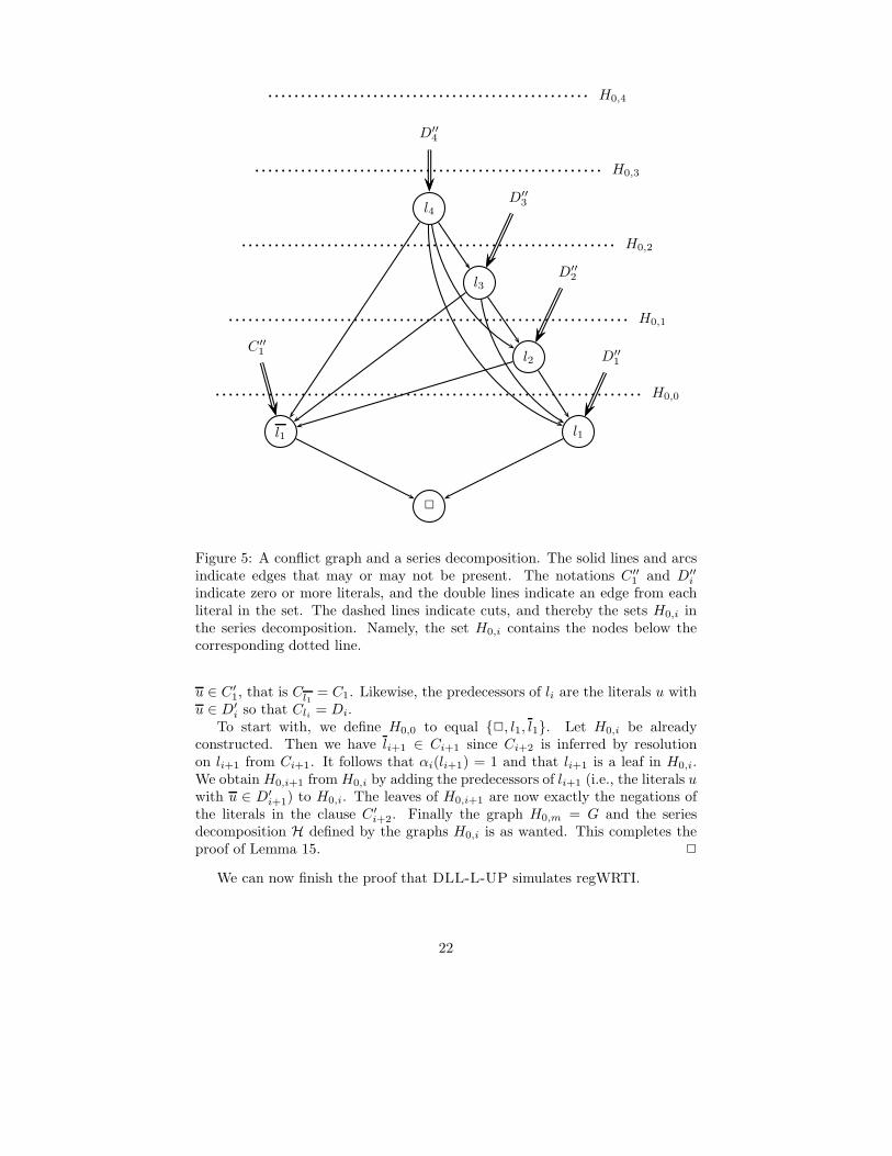
2

l4

l3

l2

l1l1

D′′1

D′′2

D′′3

D′′4

C′′1

H0,0

H0,1

H0,2

H0,3

H0,4

Figure 5: A conflict graph and a series decomposition. The solid lines and arcsindicate edges that may or may not be present. The notations C′′

1 and D′′i

indicate zero or more literals, and the double lines indicate an edge from eachliteral in the set. The dashed lines indicate cuts, and thereby the sets H0,i inthe series decomposition. Namely, the set H0,i contains the nodes below thecorresponding dotted line.

u ∈ C′1, that is Cl1

= C1. Likewise, the predecessors of li are the literals u withu ∈ D′

i so that Cli = Di.To start with, we define H0,0 to equal 2, l1, l1. Let H0,i be already

constructed. Then we have li+1 ∈ Ci+1 since Ci+2 is inferred by resolutionon li+1 from Ci+1. It follows that αi(li+1) = 1 and that li+1 is a leaf in H0,i.We obtain H0,i+1 from H0,i by adding the predecessors of li+1 (i.e., the literals uwith u ∈ D′

i+1) to H0,i. The leaves of H0,i+1 are now exactly the negations ofthe literals in the clause C′

i+2. Finally the graph H0,m = G and the seriesdecomposition H defined by the graphs H0,i is as wanted. This completes theproof of Lemma 15. 2

We can now finish the proof that DLL-L-UP simulates regWRTI.

22

Theorem 16. Suppose that F has a regWRTI proof of size s. Then there isan execution of the non-greedy DLL-L-UP algorithm with the input (F, ∅) thatmakes < s recursive calls.

Proof. Let T be a regWRTI refutation of F . The DLL-L-UP algorithm worksby traversing the proof tree T in a depth-first, left-to-right order. At eachnon-input-derived node u of T , labeled with a clause C, the resolution variablefor that clause is chosen as the branching variable x, and the variable x isassigned the value 1 or 0, corresponding to the label on the edges coming into u.By part b. of Theorem 4, the clause C is falsified by the assignment α. At eachinput-derived node of T , the DLL-L-UP algorithm learns the clauses in theinput subproof above u by using the conflict graph and series decompositiongiven by Lemma 15. Since the DLL-L-UP search cannot find a satisfyingassignment, it must terminate after traversing the (non-input) nodes in theregWRTI refutation tree. The number of recursive calls will equal twice thenumber of non-input-derived nodes of T , which is less than s. 2

6 Generalized DLL with clause learning

6.1 The algorithm DLL-Learn

This section presents a new formulation of DLL with learning called DLL-

Learn. This algorithm differs from DLL-L-UP in two important ways. First,unit propagation is no longer used explicitly (although it can be simulated).Second, the DLL-Learn algorithm uses more information that arises duringthe DLL search process, namely, it can infer clauses by resolution at each nodein the search tree. This makes it possible for DLL-Learn to simulate regularresolution trees with full lemmas; more specifically, DLL-Learn is equivalentto regWRTL.

The DLL-Learn algorithm is very similar to the pool resolution systemintroduced by Van Gelder [25]. Furthermore, our Theorem 17 is similar to resultsobtained by Van Gelder for pool resolution. Our constructions differ mostly inthat we use w-resolution in place of the degenerate resolution inference of VanGelder [25]. Loosely speaking, Van Gelder’s degenerate resolution inference isa method of allowing resolution to operate on any two clauses without anyweakening. Conversely, our w-resolution is a method for allowing resolutionto operate on any two clauses, but with the maximum reasonable amount ofweakening.

The idea of DLL-Learn is to extend DLL so that it can learn a new clause Cat each node in the search tree. As usual, the new clause will satisfy F ≡ F∪C.At leaves, DLL-Learn does not learn a new clause, but marks a preexistingfalsified clause as “new”. At internal nodes, after branching on a variable x andmaking two recursive calls, the DLL-Learn algorithm can use w-resolution toinfer a new clause, CDLL(F,α), from the two identified new clauses, C0 and C1

returned by the recursive calls. Since x does not have to occur in Var(C0)and Var(C1), C is obtained by a w-resolution instead of resolution.

23

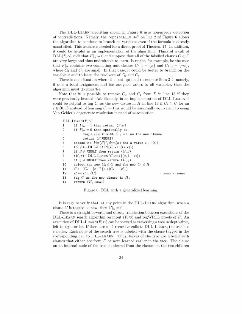
The DLL-Learn algorithm shown in Figure 6 uses non-greedy detectionof contradictions. Namely, the “optionally do” on line 2 of Figure 6 allowsthe algorithm to continue to branch on variables even if the formula is alreadyunsatisfied. This feature is needed for a direct proof of Theorem 17. In addition,it could be helpful in an implementation of the algorithm: Think of a call ofDLL(F, α) such that F |α = 0 and suppose that all of the falsified clauses C ∈ Fare very large and thus undesirable to learn. It might, for example, be the casethat F |α contains two conflicting unit clauses C0|α = x and C1|α = ¬x,where C0 and C1 are small. In that case, it could be better to branch on thevariable x and to learn the resolvent of C0 and C1.

There is one situation where it is not optional to execute lines 3-4; namely,if α is a total assignment and has assigned values to all variables, then thealgorithm must do lines 3-4.

Note that it is possible to remove C0 and C1 from F in line 13 if theywere previously learned. Additionally, in an implementation of DLL-Learn itcould be helpful to tag Ci as the new clause in H in line 13 if Ci ⊆ C for ani ∈ 0, 1 instead of learning C — this would be essentially equivalent to usingVan Gelder’s degenerate resolution instead of w-resolution.

DLL-Learn(F, α)

1 if F |α = 1 then return (F, α)

2 if F |α = 0 then optionally do

3 tag a C ∈ F with C|α = 0 as the new clause

4 return (F, UNSAT)

5 choose x ∈ Var(F ) \ dom(α) and a value ǫ ∈ 0, 16 (G, β)←DLL-Learn(F, α ∪ (x, ǫ))7 if β 6= UNSAT then return (G, β)

8 (H, γ)←DLL-Learn(G, α ∪ (x, 1− ǫ))9 if γ 6= UNSAT then return (H, γ)

10 select the new C0 ∈ G and the new C1 ∈ H

11 C ← (C0 − x1−ǫ) ∪ (C1 − x

ǫ)12 H ← H ∪ C -- learn a clause

13 tag C as the new clause in H.

14 return (H, UNSAT)

Figure 6: DLL with a generalized learning.

It is easy to verify that, at any point in the DLL-Learn algorithm, when aclause C is tagged as new, then C|α = 0.

There is a straightforward, and direct, translation between executions of theDLL-Learn search algorithm on input (F, ∅) and regWRTL proofs of F . Anexecution of DLL-Learn(F, ∅) can be viewed as traversing a tree in depth-first,left-to-right order. If there are s−1 recursive calls to DLL-Learn, the tree hass nodes. Each node of the search tree is labeled with the clause tagged in thecorresponding call to DLL-Learn. Thus, leaves of the tree are labeled withclauses that either are from F or were learned earlier in the tree. The clauseon an internal node of the tree is inferred from the clauses on the two children

24

using w-resolution with respect to the branching variable. Finally, the clause Clabeling the root node, where α = ∅, must be the empty clause, since α mustfalsify C. In this way the search algorithm describes precisely a regWRTLproof tree. Conversely, any regWRTL refutation of F corresponds exactly to anexecution of the DLL-Learn(F, ∅).

This translation between DLL-Learn and regWRTI proof trees gives thefollowing theorem.

Theorem 17. Let F be a set of clauses. There exists a regWRTL refutationof F of size s if and only if there is an execution of DLL-Learn(F, ∅) thatperforms exactly s − 1 recursive calls.

It follows as a corollary of Theorems 7 and 17 that DLL-Learn can poly-nomially simulate DLL-L-UP.

7 Variable Extensions

This section introduces the notion of a variable extension of a CNF formula. Avariable extension augments a set F of clauses with additional clauses suchthat modified formula VEx(F ) is satisfiable if and only if F is satisfiable.Variable extensions will be used to prove that regWRTI proofs can simulateresolution dags, in the sense that if there is an RD refutation of F , then thereis a polynomial size regWRTI refutation of VEx(F ). Hence, DLL-Learn andthe non-greedy version of DLL-L-UP can simulate full (non-regular) resolutionin the same sense.

Our definition of variable extensions is inspired by the proof trace extensionsof Beame et al. [3] that were used to separate DLL with clause learning fromregular resolution dags. A similar construction was used by Hertel et al. [2] toshow that pool resolution can simulate full resolution. Our results strengthenand extend the prior results by applying directly to regWRTI proofs. Moreimportantly, in contrast to proof trace extensions, variable extensions do notdepend on the size of a (possibly unknown) resolution proof but only on thenumber of variables in the formula.

Definition Let F be a set of clauses and |Var(F )| = n. The set of extensionvariables of F is EVar(F ) = q, p1, . . . , pn, where q and pi are new variables.The variable extension of F is the set of clauses

VEx (F ) = F ∪

q, l : l ∈ C ∈ F

∪

p1, p2, . . . , pn

.

Obviously VEx(F ) is satisfiable if and only if F is. Furthermore, |VEx (F )| =O(|F |).

Suppose that G is a resolution dag (RD) proof from F . We can reexpress G asa sequence of (derived) clauses C1, C2, . . . , Ct which has the following properties:(a) Ct is the final clause of G, and (b) each Ci is inferred by resolution from twoclauses D and E, where each of D and E either are in F or appear earlier inthe sequence as Cj with j < i. Basically, the sequence is an ordinary resolutionrefutation, but with the clauses from F omitted.

25

Lemma 18. Suppose that D, E ⊢x C. Then, there is an input resolution prooftree TC of the clause q from VEx (F )∪D, E such that C appears in TC andsuch that |TC | = 2 · |C| + 3.

Proof. The proof TC starts by resolving D and E to yield C. It then resolvessuccessively with the clauses q, l, for l ∈ C, to derive q. 2

Theorem 19. Let F be a set of clauses, n = |Var(F )|, and let C be a clause.Suppose that G is a resolution dag proof of C from F of size s. Then, thereis a regWRTI proof T of C from VEx(F ) of size ≤ 2s · (d + 2) + 1 whered = max|D| : D ∈ G ≤ n.

Proof. Let C1, . . . , Ct be a sequence of the derived clauses in G as above.Without loss of generality, t < 2n since F also has a regular resolution treerefutation, and this has depth at most n, and thus has < 2n internal nodes. LetT ′ be a binary tree with t leaves and of height h = ⌈log2 t⌉ ≤ n. For each node uin T ′, let l(u) be the level of u in T ′, namely, the number of edges between uand the root. Label u with the variable pl(u). Also, label every node u in T ′

with the clause q. T ′ will form the middle part of a regWRTI proof: eachclause q at level i is inferred by w-resolution from its two children clauses(also equal to q) with respect to the variable pi.

Now, we expand T ′ into a regWRTI proof tree T ′′. For this, for 1 ≤ i ≤ t, wereplace the i-th leaf of T ′ with a new subproof TCi

defined as follows. LettingCi be as above, let Di and Ei be the two clauses from which Ci is inferredin G. Then replace i-th leaf of T ′ by the input proof TCi

from Lemma 18 whichcontains Ci and ends with the clause q. Note that each of Di and Ei either isin F or appeared as an input clause in a proof, TDi

or TEi, inserted at an earlier

leaf of T ′. Therefore T ′′ is a valid regWRTI proof of q from VEx (F ). Sincethere are at most s− 1 internal nodes in T ′ and each TCi

has size ≤ 2d + 3, T ′′

has size at most (s − 1) + s · (2d + 3).Finally, we form a regWRTI proof of C by modifying T ′′ by adding a new

root labeled with the clause C and the resolution variable q. Let the left childof this new root be the root of T ′′, and let the right child be a new node labeledalso with C. (This is permissible since C is input-derived in T ′′.) Label theleft edge coming to the new root with the literal q, and the right edge with theliteral q. This makes C inferred from q and C by w-resolution with respectto q. T is a valid regWRTI of size at most s+1+s ·(2d+3) = 2s ·(d+2)+1. 2

Since DLL-L-UP and DLL-Learn simulate regWRTI, Theorem 19 impliesthat these two systems p-simulate full resolution by the use of variable exten-sions:

Corollary 20. Suppose that F has a resolution dag refutation of size s. Thenboth DLL-L-UP and DLL-Learn, when given VEx(F ) as input, have execu-tions that return UNSAT after at most p(s) recursive calls, for some polynomial p.

We now consider some issues about “naturalness” of proofs based on reso-lution with lemmas. Beame et al. [3] defined a refutation system to be natural

26

provided that, whenever F has a refutation of size s, then F |α has a refutationof size at most s. We need a somewhat relaxed version of this notion:

Definition Let R be a refutation system for sets of clauses. The system R isp-natural provided, there is a polynomial p(s), such that, whenever a set F hasan R-refutation of size s, and α is a restriction, then F |α has an R-refutationof size ≤ p(s).

The next proposition is well-known.

Proposition 21. Resolution dags (RD) and regular resolution dags (regRD)are natural proof systems.

As a corollary to Theorem 19 we obtain the following theorem.

Theorem 22.

a. regWRTI is equivalent to RD if and only if regWRTI is p-natural.

b. regWRTL is equivalent to RD if and only if regWRTL is p-natural.

Proof. Suppose that regWRTI ≡ RD. Then, since RD is natural, we haveimmediately that regWRTI is p-natural.

Conversely, suppose that regWRTI is p-natural. By Theorem 7, RD p-simulates regWRTI. So it suffices to prove that regWRTI p-simulates RD. LetF have an RD refutation of size s. By Theorem 19, VEx(F ) has a regWRTIproof of size 2s(s + 2) + 1. Let α be the assignment that assigns the value 1 toeach of the extension variables q and p1, . . . , pn. Since VEx (F )|α is F and sinceregWRTI is p-natural, F has a regWRTI proof of size at most p(2s(s + 2) + 1).This proves that regWRTI p-simulates RD, and completes the proof of a.

The proof of b. is similar. 2

Theorem 22 is stated for the equivalence of systems with RD. It could alsobe stated for p-equivalent but then one needs an “effective” version of p-natural,where the R-refutation of F |α is computable in polynomial time from α and aR-refutation of F .

8 A Lower Bound for RTLW with short lemmas

In this section we prove a lower bound showing that learning only short clausesdoes not help a DLL algorithm for certain hard formulas. The proof systemcorresponding to DLL algorithms with learning restricted to clauses of length kis, according to Section 5, regWRTI with the additional restriction that everyused lemma is a clause of length at most k. We prove a lower bound for astronger proof system that allows arbitrary lemmas instead of just input lemmas,drops the regularity restriction, and uses the general weakening rule instead ofjust w-resolution, i.e., RTLW as defined in Section 3. We define RTLW(k) to bethe restriction of RTLW in which every lemma used, i.e., every leaf label thatdoes not occur in the initial formula, is of size at most k.

27

The hard example formulas we prove the lower bound for are the well-knownPigeonhole Principle formulas. This principle states that there can be no 1-to-1mapping from a set of size n + 1 into a set of size n. In propositional logic, thenegation of this principle gives rise to an unsatisfiable set of clauses PHPn inthe variables xi,j for 1 ≤ i ≤ n + 1 and 1 ≤ j ≤ n. The variable xi,j is intendedto state that i is mapped to j. The set PHPn consists of the following clauses:

• the pigeon clause Pi =

xi,j ; 1 ≤ j ≤ n

for every 1 ≤ i ≤ n + 1.

• the hole clause Hi,j,k = xi,k, xj,k for every 1 ≤ i < j ≤ n+1 and k ≤ n.

It is well-known that the pigeonhole principle requires exponential size dag-like resolution proofs: Haken [16] shows that every RD refutation of PHPn isof size 2Ω(n). Note that the number of variables is O(n2), so that this lowerbound is far from maximal. In fact, Iwama and Miyazaki [18] prove a largerlower bound for tree-like refutations.

Theorem 23 (Iwama and Miyazaki [18]). Every resolution tree refutation ofPHPn is of size at least (n/4)n/4.

We will show that for k ≤ n/2, RTLW(k) refutations of PHPn are asymp-totically of the same size 2Ω(n log n) as resolution trees. On the other hand,it is known [8] that dag-like resolution proofs need not be much larger thanHaken’s lower bound: there exist RD refutations of PHPn of size 2n ·n2. Theserefutations are even regular, and thus can be simulated by regWRTI. HencePHPn can be solved in time 2O(n) by some variant of DLL-L-UP when learningarbitrary long clauses, whereas our lower bound shows that any DLL algorithmthat learns only clauses of size at most n/2 needs time 2Ω(n log n).

In fact, we will prove our lower bound for the weaker functional pigeonholeprinciple FPHPn, which also includes the following clauses:

• The functional clause Fi,j,k = xi,j , xi,k for every 1 ≤ i ≤ n+1 and every1 ≤ j < k ≤ n.

While the lower bound of Iwama and Miyazaki is only stated for the clausesPHPn, it is easily verified that their proof works as well when the functionalclauses are added to the formula.

Our lower bound proof uses the fact that resolution trees with weakening(RTW) are natural, i.e., preserved under restrictions in the following sense:

Proposition 24. Let R be a RTW proof of C from F of size s, and ρ arestriction. There is an RTW proof R′ for C|ρ from F |ρ of size at most s.

We denote the resolution tree R′ by R|ρ. Since this proposition is well-knowna proof will not be given.

Next, we need to bring refutations in RTLW(k) to a certain normal form.First, we show that it is unnecessary to use clauses as lemmas that are subsumedby axioms in the refuted formula.

28

Lemma 25. If there is a RTLW(k) refutation of some formula F of size s,then there is a RTLW(k) refutation of F of size at most 2s in which no clauseC with C ⊇ D for some clause D in F is used as a lemma.

Proof. If a clause C with C ⊇ D for some D ∈ F is used as a lemma, replaceevery leaf labeled C by a weakening inference of C from D. 2

Secondly, we need the fact that an RTLW(k) refutation does not need to useany tautological clauses, i.e., clauses of the form C ∪ x, x for a variable x.

Lemma 26. If there is a RTLW(k) refutation of some formula F of size s,then there is a RTLW(k) refutation of F of size at most s that contains notautological clause.

Proof. Let P be an RTLW(k)-refutation of F of size s that contains t occurrencesof tautological clauses. We transform P into a refutation P ′ of size |P ′| ≤ ssuch that P ′ contains fewer than t occurrences of tautological clauses. Finitelymany iterations of this process yields the claim.

We obtain P ′ as follows. Since the final clause of P is not tautological, ift > 0, there must be a tautological clause C ∪ x, x which is resolved with aclause D∪x to yield a non-tautological clause C ∪D∪x. The idea is to cutout the subtree T0 that derives the clause C ∪ x, x, and derive C ∪ D ∪ xby a weakening from D ∪ x. This gives a “proof” P0 with fewer tautologicalclauses than P . However, P0 may not be a valid proof, since some of the clausesin T0 might be used as lemmas in P0. To fix this, we shall extract parts of T0

and plant them onto P0 so that all lemmas used are derived. In order to makethis construction precise, we need the notion of trees in which some of the usedlemmas are not derived.

A partial RTLW from F is defined to be a tree T which satisfies all theconditions of an RTLW, except that some leaves may be labeled by clauses thatoccur neither in F nor earlier in T ; these are called the open leaves of T .

We construct P ′ in stages by defining, for i ≥ 0, a partial RTLW refutation Pi

of F and a partial RTLW derivation Ti of C ∪ x, x from F with the followingproperties:

• All open leaves in Pi appear in Ti. The first open leaf in Pi is denoted Ci.

• All open leaves in Ti appear in Pi before Ci.

• |Pi| + |Ti| = |P | .

P0 and T0 were defined above and certainly satisfy the two properties. GivenPi and Ti, we construct Pi+1 and Ti+1 as follows: We locate the first occurrenceof Ci in Ti and let T ∗

i be the subtree of Ti rooted at this occurrence. We formTi+1 by replacing in Ti the subtree T ∗

i by a leaf labeled Ci. And, we form Pi+1

by replacing the first open leaf, Ci, in Pi by the tree T ∗i .

The invariants are easily seen to be preserved. Obviously, |Pi+1| + |Ti+1| =|Pi| + |Ti| = |P |. The open leaves of T ∗

i appear in Pi before Ci, and therefore,any open leaf in Pi+1, and in particular, Ci+1 if it exists, must occur after the

29

(formerly open leaf) clause Ci. New open leaves in Ti are Ci and possibly somelemmas derived in T ∗

i , and these all occur in Pi+1 before Ci+1.Since Pi+1 contains fewer open leaves than Pi for every i, there is an m such

that Pm contains no open leaves, and thus is an RTLW refutation. We thendiscard Tm and set P ′ := Pm. Each lemma used in P ′ was a lemma in P , thusP ′ is also an RTLW(k) refutation.

Note that the total number of occurrences of tautological clauses in Pi+1

and Ti+1 combined is the same as in Pi and Ti combined. This is also equal tothe number of tautological clauses in P . Furthermore, Tm must contain at leastone tautological clause, namely its root C ∪ x, x. It follows that P ′ has fewertautological clauses than P . 2

A matching ρ is a set of pairs

(i1, j1), . . . , (ik, jk)

⊂ 1, . . . , n + 1 ×1, . . . , n such that all the iν as well as all the jν are pairwise distinct. Thesize of ρ is |ρ| = k. A matching ρ induces a partial assignment to the variablesof PHPn as follows:

ρ(xi,j) =

1 if (i, j) ∈ ρ

0 if there is (i, j′) ∈ ρ with j 6= j′

or (i′, j) ∈ ρ with i 6= i′

undefined otherwise.

We will identify a matching and the assignment it induces. The crucial propertyof such a matching restriction ρ is that FPHPn|ρ is – up to renaming of variables– the same as FPHPn−|ρ|.

The next lemma states that a short clause occurring as a lemma in an RTLWrefutation can always be falsified by a small matching restriction.

Lemma 27. Let C be a clause of size k ≤ n/2 such that

• C is not tautological,

• C 6⊇ Hi,i′,j for any hole clause Hi,i′,j,

• C 6⊇ Fi,j,j′ for any functional clause Fi,j,j′ .

Then there is a matching ρ of size |ρ| ≤ k such that C|ρ = 2.

Proof. First, we let ρ1 consist of all those pairs (i, j) such that the negativeliteral xi,j occurs in C. By the second and third assumption, these pairs forma matching. All the negative literals in C are set to 0 by ρ1, and by the firstassumption, no positive literal in C is set to 1 by ρ1.

Now consider all pigeons i1, . . . , ir mentioned in positive literals in C thatare not already set to 0 by ρ1, i.e., that are not mentioned in any of the negativeliterals in C. Pick j1, . . . , jr from the n/2 holes not mentioned in C, and setρ2 :=

(i1, j1), . . . , (ir, jr)

. This matching sets the remaining positive literalsto 0, thus for ρ := ρ1 ∪ ρ2, we have C|ρ = 2. Clearly the size of ρ is at most ksince we have picked at most one pair for each literal in C. 2

30

Finally, we are ready to put all ingredients together to prove our lower bound.

Theorem 28. For every k ≤ n/2, every RTLW(k)-refutation of FPHPn is ofsize 2Ω(n log n).

Proof. Let R be an RTLW(k)-refutation of FPHPn of size s. By Lemmas 25and 26, R can be transformed into R′ of size at most 2s in which no clause istautological and no clause used as a lemma is subsumed by a clause in FPHPn.Let C be the first clause in R′ which is used as a lemma; C is of size at most k.The subtree RC of R′ rooted at C is a resolution tree for C from FPHPn.

By Lemma 27, there is a matching restriction ρ of size |ρ| ≤ k such thatC|ρ = 2. Then RC |ρ is a resolution tree with weakening refutation of FPHPn|ρ,which is the same as FPHPn−k. By Proposition 3, applications of the weakeningrule can be eliminated from RC |ρ without increasing the size. Therefore byTheorem 23, RC is of size

(n − k

4

)n−k

4

≥(n

8

)n8

and hence the size of R is at least

s ≥1

2|RC | ≥ 2Ω(n log n).

2

References

[1] Michael Alekhnovich, Jan Johannsen, Toniann Pitassi, and AlasdairUrquhart. An exponential separation between regular and general reso-lution. Theory of Computing, 3:81–102, 2007.

[2] Fahim Bacchus, Philipp Hertel, Toniann Pitassi, and Allen Van Gelder.Clause learning can effectively p-simlulate general propositional resolution.Submitted for publication, 2008.

[3] Paul Beame, Henry A. Kautz, and Ashish Sabharwal. Towards understand-ing and harnessing the potential of clause learning. J. Artif. Intell. Res.(JAIR), 22:319–351, 2004.

[4] Daniel Le Berre and Laurent Simon. The essentials of the SAT 2003 com-petition. In Proc. 6th International Conference on Theory and Applicationsof Satisfiability (SAT 2003), LNCS 2919, pages 452–467. Springer, 2003.

[5] Daniel Le Berre and Laurent Simon. Fifty-five solvers in Vancouver: TheSAT 2004 competition. In Theory and Applications of Satisfiability Test-ing: 7th International Conference, SAT 2004, LNCS 3542, pages 321–344.Springer, 2004.

31

[6] Daniel Le Berre and Laurent Simon. Preface to the special volume on theSAT 2005 competitions and evaluations. Journal on Satisfiability, BooleanModeling and Computation, 2:i–xiv, 2005.

[7] Maria Luisa Bonet, Juan Luis Esteban, Nicola Galesi, and Jan Johannsen.On the relative complexity of resolution restrictions and cutting planesproof systems. SIAM Journal on Computing, 30:1462–1484, 2000.

[8] Samuel R. Buss and Toniann Pitassi. Resolution and the weak pigeonholeprinciple. In Mogens Nielsen and Wolfgang Thomas, editors, Computer Sci-ence Logic, 11th International Workshop CSL ’97, pages 149–156. SpringerLNCS 1414, 1998.

[9] C. L. Chang. The unit proof and the input proof in theorem proving. J.ACM, 17(4):698–707, 1970.

[10] Martin Davis, George Logemann, and Donald W. Loveland. A machineprogram for theorem-proving. Commun. ACM, 5(7):394–397, 1962.

[11] Martin Davis and Hilary Putnam. A computing procedure for quantifica-tion theory. J. ACM, 7(3):201–215, 1960.

[12] Niklas Een and Armin Biere. Effective preprocessing in SAT throughvariable and clause elimination. In Proc. 8th International Conference onTheory and Applications of Satisfiability Testing (SAT’05), LNCS 3569,pages 61–75. Springer, 2005.

[13] Jon W. Freeman. Improvements to Propositional Satisfiability Search Al-gorithms. PhD thesis, University of Pennsylvania, Philadelphia, PA, USA,1995.

[14] Zhaohui Fu, Yogesh Mahajan, and Sharad Malik. New features of theSAT’04 version of zChaff. SAT Competition 2004 – Solver Description,http://www.princeton.edu/ chaff/zchaff/sat04.pdf, 2004.

[15] Andreas Goerdt. Regular resolution versus unrestricted resolution. SIAMJ. Comput., 22(4):661–683, 1993.

[16] Armin Haken. The intractability of resolution. Theor. Comput. Sci.,39:297–308, 1985.

[17] Jan Hoffmann. Resolution proofs and DLL-algorithms with clause learning.Diploma Thesis, LMU Munchen, 2007. http://www.tcs.ifi.lmu.de/

~hoffmann .

[18] Kazuo Iwama and Shuichi Miyazaki. Tree-like resolution is superpolynomi-ally slower than dag-like resolution for the pigeonhole principle. In Proceed-ings of the 10th International Symposium on Algorithms and Computation(ISAAC), pages 133–142, 1999.

32

[19] Roberto J. Bayardo Jr. and Robert C. Schrag. Using CSP look-back tech-niques to solver real-world SAT instances. In Proc. 14th Natl. Conferenceon Artificial Intelligence, pages 203–208, 1997.

[20] Yogesh S. Mahajan, Zhaohui Fu, and Sharad Malik. Zchaff2004: An effi-cient SAT solver. In Theory and Applications of Satisfiability Testing: 7thInternational Conference, SAT 2004, LNCS 3542, pages 360–375. Springer,2004.

[21] Matthew W. Moskewicz, Conor F. Madigan, Ying Zhao, Lintao Zhang, andSharad Malik. Chaff: Engineering an efficient SAT solver. In Proc. 38thDesign Automation Conference (DAC’01), pages 530–535, 2001.

[22] Alexander Nadel. Backtrack search algorithms for propositional logic sat-isfiability: Review and innovations. Master’s thesis, Hebrew University ofJerusalem, Israel, 2002.

[23] Joao P. Marques Silva and Karem A. Sakallah. GRASP - a new searchalgorithm for satisfiability. In Proc. IEEE/ACM International Conferenceon Computer Aided Design (ICCAD), pages 220–227, 1996.

[24] G.S. Tseitin. On the complexity of derivation in propositional calculus.Studies in Constructive Mathematics and Mathematical Logic, Part 2,pages 115–125, 1968.

[25] Allen Van Gelder. Pool resolution and its relation to regular resolutionand DPLL with clause learning. In Logic for Programming, ArtificialIntelligence, and Reasoning (LPAR), LNAI 3835, pages 580–594, MontegoBay, Jamaica, 2005. Springer-Verlag.

[26] Lintao Zhang, Conor F. Madigan, Matthew W. Moskewicz, and SharadMalik. Efficient conflict driven learning in a Boolean satisfiability solver.In Proc. IEEE/ACM International Conference on Computer Aided Design(ICCAD), pages 279–285, 2001.

33