PNNL-22182

Residential Lighting End-Use Consumption Study: Estimation Framework and Initial Estimates

WR Gifford1

ML Goldberg2

PM Tanimoto2

DR Celnicker1

ME Poplawski3

December 2012

Prepared for the U.S. Department of Energy under Contract DE-AC05-76RL01830

Prepared by DNV KEMA Energy and Sustainability Pacific Northwest National Laboratory

1 DNV KEMA Energy and Sustainability, Fairfax, Virginia 2 DNV KEMA Energy and Sustainability, Madison, Wisconsin 3 Pacific Northwest National Laboratory, Portland, Oregon

Executive Summary

The U.S. DOE Residential Lighting End-Use Consumption Study is an initiative of the U.S. Department of Energy’s (DOE’s) Solid-State Lighting Program that aims to improve the understanding of lighting energy usage in residential dwellings. The study has developed a regional estimation framework within a national sample design that allows for the estimation of lamp usage and energy consumption 1) nationally and by region of the United States, 2) by certain household characteristics, 3) by location within the home, 4) by certain lamp characteristics, and 5) by certain categorical cross-classifications (e.g., by dwelling type AND lamp type or fixture type AND control type).

The lighting estimates presented in this report leverage several recent national and regional datasets, linking lamp usage from end-use metering studies with household characteristics and lighting inventory profiles that are anchored to a robust regionally stratified national sample design. The lighting usage measures were estimated using a “bottom-up” methodology, in that lamp power, hours-of-use (HOU), and energy consumption estimates were generated at the lamp level and aggregated up to various levels of analysis. It should be noted that the statistical model for lamp usage came from a single regional study that has not yet been calibrated for other regions of the United States.1 For many regions, neither a local study nor direct reporting in a national survey was available for use in this analysis, so extrapolations were made based on the information known from neighboring or nearby regions. The available lighting inventory data available from the South census region were noticeably limited. Lighting inventory data averaged across all regions were assigned to homes in locations without regionally specific data.

This study produced lighting estimates based on existing data. However, the estimation framework was designed to make straightforward use of new data collected under similar protocols. For example, if a state or regional organization conducted a lighting study using protocols for the collection of household characteristics, lighting inventories, and/or the end-use metering of fixtures that would support linkages of the collected data to the data sources being used in this study, then the new data could be easily incorporated into the developed estimation framework. Lighting usage estimates could then be updated, resulting in improved regional and possibly national accuracy. The estimates presented in this report include a validation of the accuracy achieved in California using the described process for linking newly collected data. Updates to this study will be considered if enough new data meeting the described pre-conditions and funding for its analysis were to become available.

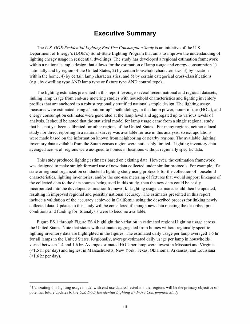
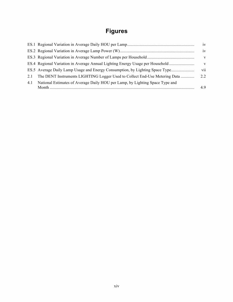
Figure ES.1 through Figure ES.4 highlight the variation in estimated regional lighting usage across the United States. Note that states with estimates aggregated from homes without regionally specific lighting inventory data are highlighted in the figures. The estimated daily usage per lamp averaged 1.6 hr for all lamps in the United States. Regionally, average estimated daily usage per lamp in households varied between 1.4 and 1.6 hr. Average estimated HOU per lamp were lowest in Missouri and Virginia (<1.5 hr per day) and highest in Massachusetts, New York, Texas, Oklahoma, Arkansas, and Louisiana (>1.6 hr per day).

1 Calibrating this lighting usage model with end-use data collected in other regions will be the primary objective of potential future updates to the U.S. DOE Residential Lighting End-Use Consumption Study.

iii

* Note: Lighting inventory data for this state or its neighbor was not available.

Figure ES.1. Regional Variation in Average Daily HOU per Lamp

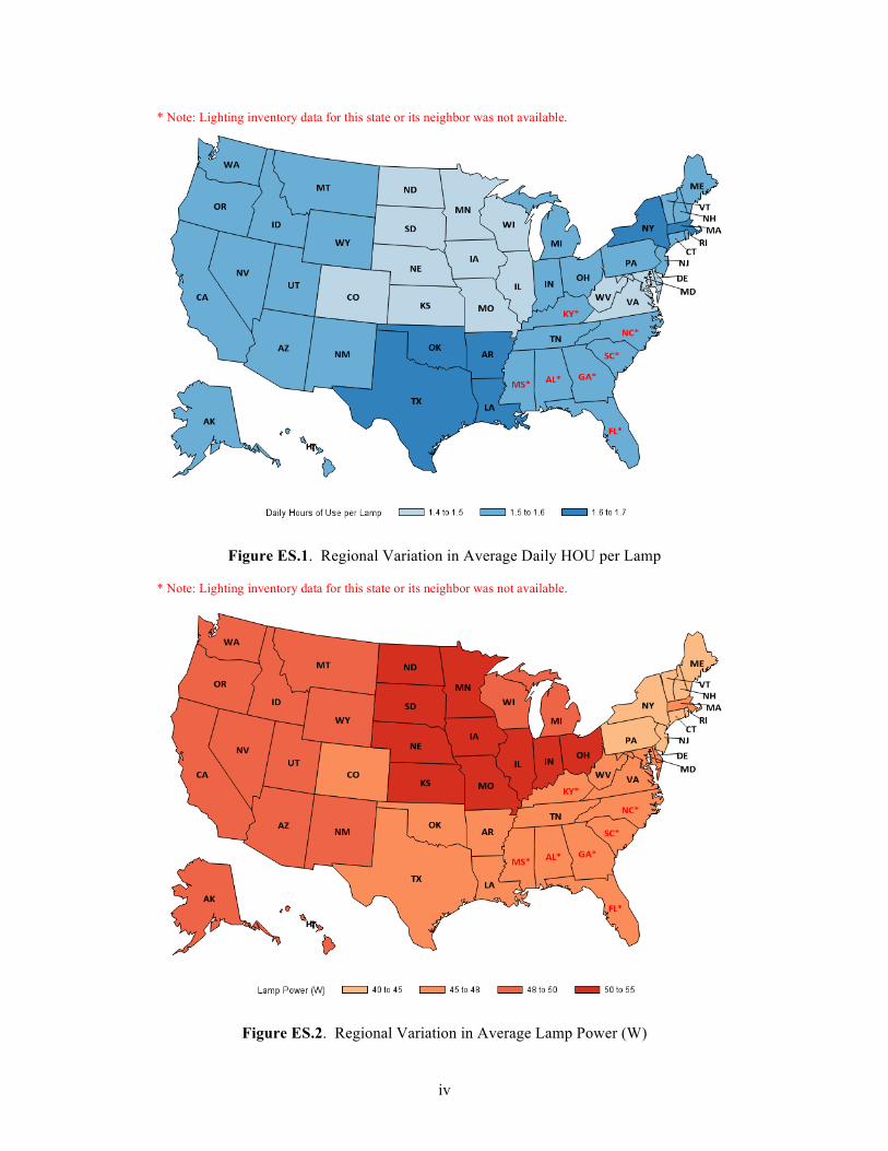
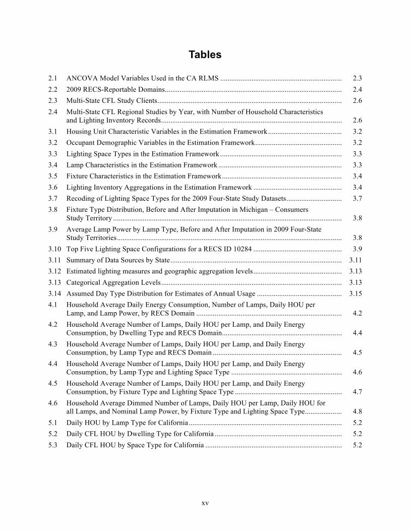
* Note: Lighting inventory data for this state or its neighbor was not available.

Figure ES.2. Regional Variation in Average Lamp Power (W)

iv

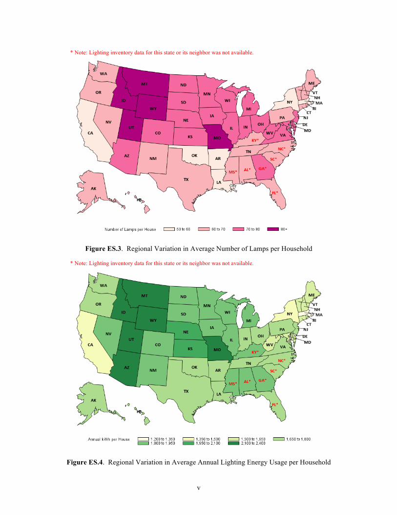
* Note: Lighting inventory data for this state or its neighbor was not available.

Figure ES.3. Regional Variation in Average Number of Lamps per Household

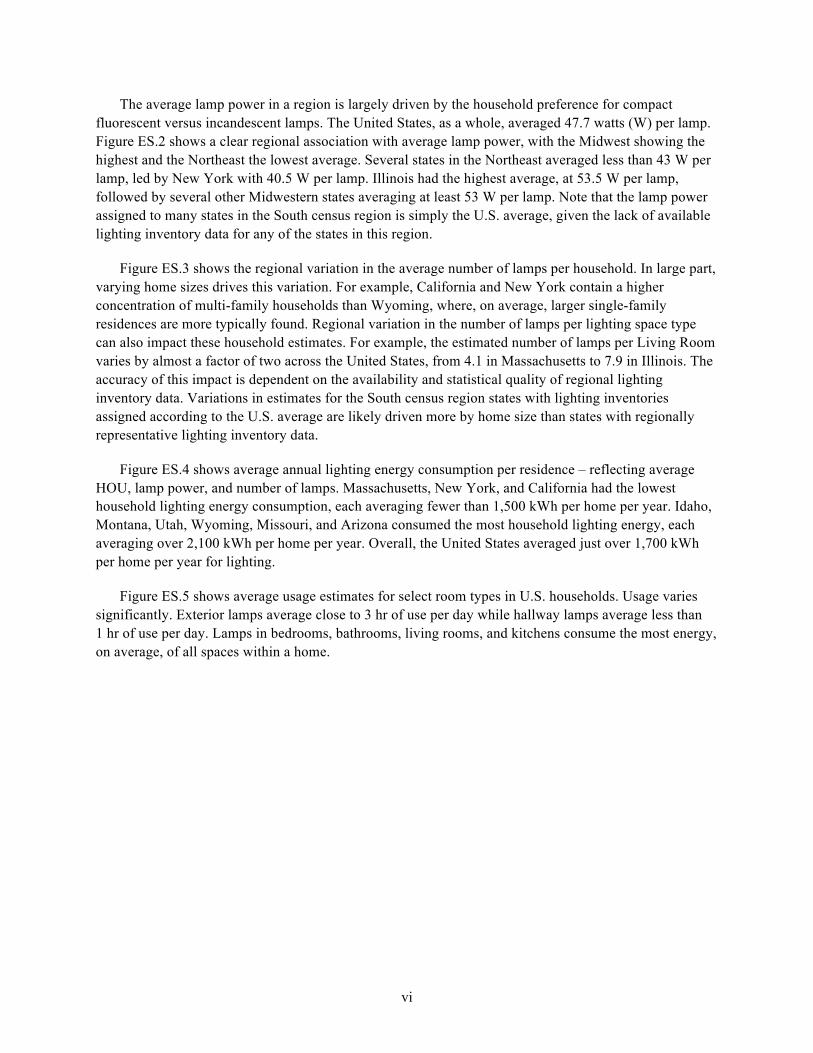
* Note: Lighting inventory data for this state or its neighbor was not available.

Figure ES.4. Regional Variation in Average Annual Lighting Energy Usage per Household

v

The average lamp power in a region is largely driven by the household preference for compact fluorescent versus incandescent lamps. The United States, as a whole, averaged 47.7 watts (W) per lamp. Figure ES.2 shows a clear regional association with average lamp power, with the Midwest showing the highest and the Northeast the lowest average. Several states in the Northeast averaged less than 43 W per lamp, led by New York with 40.5 W per lamp. Illinois had the highest average, at 53.5 W per lamp, followed by several other Midwestern states averaging at least 53 W per lamp. Note that the lamp power assigned to many states in the South census region is simply the U.S. average, given the lack of available lighting inventory data for any of the states in this region.

Figure ES.3 shows the regional variation in the average number of lamps per household. In large part, varying home sizes drives this variation. For example, California and New York contain a higher concentration of multi-family households than Wyoming, where, on average, larger single-family residences are more typically found. Regional variation in the number of lamps per lighting space type can also impact these household estimates. For example, the estimated number of lamps per Living Room varies by almost a factor of two across the United States, from 4.1 in Massachusetts to 7.9 in Illinois. The accuracy of this impact is dependent on the availability and statistical quality of regional lighting inventory data. Variations in estimates for the South census region states with lighting inventories assigned according to the U.S. average are likely driven more by home size than states with regionally representative lighting inventory data.

Figure ES.4 shows average annual lighting energy consumption per residence – reflecting average HOU, lamp power, and number of lamps. Massachusetts, New York, and California had the lowest household lighting energy consumption, each averaging fewer than 1,500 kWh per home per year. Idaho, Montana, Utah, Wyoming, Missouri, and Arizona consumed the most household lighting energy, each averaging over 2,100 kWh per home per year. Overall, the United States averaged just over 1,700 kWh per home per year for lighting.

Figure ES.5 shows average usage estimates for select room types in U.S. households. Usage varies significantly. Exterior lamps average close to 3 hr of use per day while hallway lamps average less than 1 hr of use per day. Lamps in bedrooms, bathrooms, living rooms, and kitchens consume the most energy, on average, of all spaces within a home.

vi

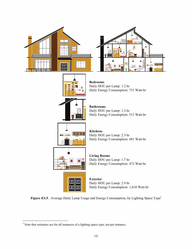
Bedrooms Daily HOU per Lamp: 1.2 hr Daily Energy Consumption: 751 Watt-hr

Bathrooms Daily HOU per Lamp: 1.2 hr Daily Energy Consumption: 512 Watt-hr

Kitchens Daily HOU per Lamp: 2.3 hr Daily Energy Consumption: 481 Watt-hr

Living Rooms Daily HOU per Lamp: 1.7 hr Daily Energy Consumption: 472 Watt-hr

Exterior Daily HOU per Lamp: 2.9 hr Daily Energy Consumption: 1,610 Watt-hr

Figure ES.5. Average Daily Lamp Usage and Energy Consumption, by Lighting Space Type1

1 Note that estimates are for all instances of a lighting space type, not per instance.

vii

Acknowledgments

The authors would like to thank the following individuals, who contributed to this study in various ways, including: review of the method, results and report; assistance obtaining data used in the analysis; insight into data used in the analysis; and guidance in structuring the framework such that it could be extended to incorporate additional data and improve estimation accuracy:

• Dan Chwastyk – Navigant

• Ed Cureg – U.S. Energy Information Administration

• Kelly Gordon – Pacific Northwest National Laboratory

• Marc Ledbetter – Pacific Northwest National Laboratory

• Thomas Leckey – U.S. Energy Information Administration

• Hiroaki Minato – U.S. Energy Information Administration

• Michael Myer – Pacific Northwest National Laboratory

• Eileen O’Brien – U.S. Energy Information Administration

• Lisa Wilson-Wright – Nexus Market Research

The authors would also like to thank the following organizations that sponsored collection of certain data used in the study and granted their permission to use this data in the development of the estimation framework and baseline estimates:

• Ameren IU (Illinois)

• Ameren UE (Missouri)

• California Public Utilities Commission (CPUC)

• ComEd (Illinois)

• Connecticut Energy Efficiency Board

• Consumers Energy (Michigan)

• Dayton Power and Light

• Maryland Public Service Commission (EmPower Program)

• Massachusetts ENERGY STAR Lighting Program Administrators

• National Grid Rhode Island

• New York State Energy Research and Development Authority (NYSERDA)

• Salt River Project

• Wisconsin Public Service Commission

ix

CV

Acronyms and Abbreviations

AHS American Housing Survey ANCOVA analysis of covariance CA RLMS California Residential Lighting Metering Study CFL compact fluorescent light CPUC California Public Utilities Commission

coefficient of variation DOE U.S. Department of Energy EIA U.S. Energy Information Administration HOU hours of use HUD U.S. Department of Housing and Urban Development IOU Investor-Owned Utility LMC Lighting Market Characterization NMR Nexus Market Research Group, Inc. PNNL Pacific Northwest National Laboratory RECS (EIA) Residential Energy Consumption Survey

xi

Contents

Executive Summary .............................................................................................................................. iii Acknowledgments................................................................................................................................. ix

Acronyms and Abbreviations................................................................................................................ xi 1.0 Introduction................................................................................................................................... 1.1

2.0 Data Sources ................................................................................................................................. 2.1

2.1 California Residential Lighting Metering Study .................................................................. 2.1

2.2 Residential Energy Consumption Survey ............................................................................ 2.4

2.3 American Housing Survey ................................................................................................... 2.5

2.4 Nexus Market Research Group Multi-State CFL Modeling Study...................................... 2.5

2.5 Consideration of Additional Data Sources........................................................................... 2.7

3.0 Methodology................................................................................................................................. 3.1

3.1 Estimation Framework Characteristics ................................................................................ 3.1

3.1.1 Household Characteristic Variables .......................................................................... 3.1

3.1.2 Lighting Inventory Variables .................................................................................... 3.3

3.1.3 Regional Variables .................................................................................................... 3.4

3.2 Input Dataset Preparation ..................................................................................................... 3.5

3.2.1 2009 RECS Microdata .............................................................................................. 3.5

3.2.2 2009 AHS Microdata ................................................................................................ 3.5

3.2.3 2009-2010 Multi-State CFL Study Microdata .......................................................... 3.6

3.3 Combining Datasets ............................................................................................................. 3.8

3.3.1 Extending RECS Housing Units with AHS Data...................................................... 3.8

3.3.2 Extending RECS Housing Units with Multi-State CFL Study Data......................... 3.10

3.3.3 Estimation Framework Summary.............................................................................. 3.10

3.4 Lighting Estimates................................................................................................................ 3.13

3.4.1 Lamp Usage and Energy Consumption..................................................................... 3.14

3.4.2 Seasonal Variation..................................................................................................... 3.16

3.4.3 Number of Fixtures and Lamps................................................................................. 3.16

4.0 Initial Estimation Highlights......................................................................................................... 4.1

4.1 Total Energy Consumption .................................................................................................. 4.1

4.2 Lamp-Level Attributes ......................................................................................................... 4.3

5.0 Accuracy and Validity of the Estimates ....................................................................................... 5.1

5.1 Comparison with CA RLMS Estimates ............................................................................... 5.1

5.2 Statistical Precision of Estimates ......................................................................................... 5.2

5.3 Sources of Bias and Variability Introduced in the Estimates............................................... 5.3

5.4 Opportunities for Improving Estimates................................................................................ 5.4

xiii

Figures

ES.1 Regional Variation in Average Daily HOU per Lamp................................................................ iv

ES.2 Regional Variation in Average Lamp Power (W)....................................................................... iv

ES.3 Regional Variation in Average Number of Lamps per Household ............................................. v

ES.4 Regional Variation in Average Annual Lighting Energy Usage per Household ........................ v

ES.5 Average Daily Lamp Usage and Energy Consumption, by Lighting Space Type...................... vii 2.1 The DENT Instruments LIGHTING Logger Used to Collect End-Use Metering Data ............. 2.2

4.1 National Estimates of Average Daily HOU per Lamp, by Lighting Space Type and Month .......................................................................................................................................... 4.9

xiv

Tables

2.1 ANCOVA Model Variables Used in the CA RLMS .................................................................. 2.3

2.2 2009 RECS-Reportable Domains................................................................................................ 2.4

2.3 Multi-State CFL Study Clients.................................................................................................... 2.6

2.4 Multi-State CFL Regional Studies by Year, with Number of Household Characteristics and Lighting Inventory Records.................................................................................................. 2.6

3.1 Housing Unit Characteristic Variables in the Estimation Framework........................................ 3.2

3.2 Occupant Demographic Variables in the Estimation Framework............................................... 3.2

3.3 Lighting Space Types in the Estimation Framework .................................................................. 3.3

3.4 Lamp Characteristics in the Estimation Framework ................................................................... 3.3

3.5 Fixture Characteristics in the Estimation Framework................................................................. 3.4

3.6 Lighting Inventory Aggregations in the Estimation Framework ................................................ 3.4

3.7 Recoding of Lighting Space Types for the 2009 Four-State Study Datasets.............................. 3.7

3.8 Fixture Type Distribution, Before and After Imputation in Michigan – Consumers Study Territory ............................................................................................................................ 3.8

3.9 Average Lamp Power by Lamp Type, Before and After Imputation in 2009 Four-State Study Territories.......................................................................................................................... 3.8

3.10 Top Five Lighting Space Configurations for a RECS ID 10284 ................................................ 3.9

3.11 Summary of Data Sources by State............................................................................................. 3.11

3.12 Estimated lighting measures and geographic aggregation levels................................................ 3.13

3.13 Categorical Aggregation Levels.................................................................................................. 3.13

3.14 Assumed Day Type Distribution for Estimates of Annual Usage .............................................. 3.15

4.1 Household Average Daily Energy Consumption, Number of Lamps, Daily HOU per Lamp, and Lamp Power, by RECS Domain ............................................................................... 4.2

4.2 Household Average Number of Lamps, Daily HOU per Lamp, and Daily Energy Consumption, by Dwelling Type and RECS Domain................................................................. 4.4

4.3 Household Average Number of Lamps, Daily HOU per Lamp, and Daily Energy Consumption, by Lamp Type and RECS Domain ...................................................................... 4.5

4.4 Household Average Number of Lamps, Daily HOU per Lamp, and Daily Energy Consumption, by Lamp Type and Lighting Space Type ............................................................ 4.6

4.5 Household Average Number of Lamps, Daily HOU per Lamp, and Daily Energy Consumption, by Fixture Type and Lighting Space Type .......................................................... 4.7

4.6 Household Average Dimmed Number of Lamps, Daily HOU per Lamp, Daily HOU for all Lamps, and Nominal Lamp Power, by Fixture Type and Lighting Space Type.................... 4.8

5.1 Daily HOU by Lamp Type for California ................................................................................... 5.2

5.2 Daily CFL HOU by Dwelling Type for California ..................................................................... 5.2

5.3 Daily CFL HOU by Space Type for California .......................................................................... 5.2

xv

1.0 Introduction

The U.S. Residential Lighting End-Use Consumption Study aimed to develop reliable estimates of residential lamp usage and energy consumption at both national and regional levels. Multiple approaches for pursuing this goal were investigated, exploring tradeoffs in accuracy, flexibility, and required time – or associated cost. The chosen methodology prioritized flexibility, meaning here the ease of incorporating new data that might become available in the future. As a result, this effort is best described as the application of lamp hours-of-use (HOU) models to a newly developed regional estimation framework that represents the U.S. housing stock. The estimation framework is simply a constructed set of sample housing units. Each sample housing unit in the estimation framework is described by its household characteristics (including both housing unit and occupant demographic data) and lighting inventory. This estimation framework is capable of producing regional and national estimates of lighting usage and energy consumption for the entire United States, and incorporating new regional data (that meet defined pre-conditions) for calibrating the HOU models to improve estimation accuracy. This report describes the development of the estimation framework and the application of the HOU models to the framework, presents a limited set of lighting estimates, and discusses the accuracy and validity of the presented estimates. A companion Microsoft Excel spreadsheet contains the full set of estimates produced by this study, including average number of fixtures, number of lamps, daily HOU per lamp by month, lamp power, daily energy consumption, and annual energy consumption. The spreadsheet is organized to allow the estimates to be easily filtered to various levels of aggregation, and by various household and lamp characteristics and categorical cross-classifications.

Several national and regional studies that occurred between 2008 and 2010 and collected household characteristics, lighting inventory profiles, and/or lighting end-use metering data were evaluated for use in developing the HOU models and estimation framework. This study heavily leverages the recent California Residential Lighting Metering Study (CA RLMS) and U.S. Energy Information Administration (EIA) Residential Energy Consumption Survey (RECS) datasets. The estimation framework is rooted in the 2009 RECS housing sample, and the analysis of covariance (ANCOVA) HOU models developed for the 2008-2009 CA RLMS were used to estimate lighting usage for each lamp type (e.g., incandescent, compact fluorescent light [CFL], or other type). These and other datasets used in this study are described in more detail in Section 2.0. Section 3.0 explains the creation of the estimation framework, a combined dataset containing all the input variables required by the ANCOVA HOU models, and the challenges in constructing housing unit samples with household characteristics and lighting inventory data that are as regionally specific as possible. The methods used to apply the models to the estimation framework, generate lamp-level usage and energy consumption estimates, and aggregate those and other estimates to various levels are also discussed here. Section 4.0 presents a limited set of lamp usage and related energy consumption estimates. These estimates were selected to demonstrate the ability of the estimation framework to generate estimates at regional levels of aggregation and with categorical cross-classifications. Section 5.0 discusses how the standard error is calculated for all estimates and the data quality flag in the companion spreadsheet. The section concludes with examples of how the lighting usage model might be calibrated with end-use data collected in other regions, which represents the primary objective of potential future updates to the U.S. Residential Lighting End-Use Consumption Study.

All estimates presented in this study are bottom-up, in that they are derived from the lamp and fixture level within rooms of a housing unit sample, up to the desired level of analysis. Energy consumption is computed (as the product of lamp power and lamp HOU) at the lowest level and then aggregated up using

1.1

sampling weights. Top-down estimates of energy consumption, on the other hand, are the products of weighted averages of lamp power and HOU. In general, top-down and bottom-up estimates will not match, because the average of products usually differs from the product of averages. Bottom-up estimates are typically more accurate, because the paired relationship between lamp power and HOU is preserved.

For example, suppose one desired to compute the energy consumption of a group of three lamps:

Lamp 1: 100 W, 1.0 HOU per day Lamp 2: 20 W, 1.5 HOU per day Lamp 3: 30 W, 2.0 HOU per day

Bottom-Up Energy Consumption = (100 W × 1.0 HOU) + (20 W × 1.5 HOU) + (30 W × 2.0 HOU) = 190 Watt-hr

Top-Down Energy Consumption = 3 Lamps × Average Lamp Power × Average HOU = 3 Lamps × (100 + 20 + 30 W) / 3 × (1.0 + 1.5 + 2.0 HOU) / 3 = 3 Lamps × 50 Watts/Lamp × 1.5 HOU = 225 Watt-hr

Although estimation accuracy is enhanced by the bottom-up approach facilitated by the estimation framework, it is still limited by the viability of the statistical HOU model, which comes from a single regional study that has not yet been calibrated for other regions of the United States. However, the CA RLMS dataset used to create this model comes from perhaps the most comprehensive and statistically rigorous lighting inventory and end-use metering study to date. The CA RLMS dataset contains complete inventories for all lamp types collected in more than 1,200 California households and end-use metering data for a random sampling of up to seven fixtures (each containing one or more lamps) per home, for a period of several months. Although the actual bias in the estimates presented in this study is unknown, the statistical precision of the estimates can be quantified.

1.2

2.0 Data Sources

This study applies lamp HOU models to an estimation framework to generate regional and national estimates of lighting usage and energy consumption. Many datasets were identified and explored for use in constructing both the HOU models and estimation framework. The CA RLMS showed that the development of an accurate model requires many variables, spanning both household characteristic and lighting inventory data, and more than can be found in any one national residential stock assessment, (e.g., the RECS). Each ANCOVA model requires a dataset containing household characteristics, lighting inventory data, and end-use metering data. The collection of such data is both time-consuming and expensive, which largely accounts for the limited number and size of studies that meet these criteria. An estimation framework was therefore constructed, consisting of a representative sample of U.S. residences, each of which is described by household characteristic and lighting inventory variables that are used in the HOU model.

The RECS and other survey results show that household characteristics vary by region, which both justifies the estimation of lamp usage and energy consumption at regional levels of aggregation, and suggests the need to acquire data for HOU variables not in the RECS dataset at ideally the same regional levels. Although merging several smaller studies allows for the creation of more robust models and greater regional specificity, the validity of such an approach and the accuracy of results derived from the combined dataset is highly dependent on how consistent each data type is across the studies – which is a function of how well the data collection protocols match. During the analysis of the various datasets identified as candidates for use in this study, it was determined that re-categorizing household characteristic and lighting inventory data was onerous, but possible. Conversely, it was decided that ensuring end-use metering data from different datasets were of similar accuracy and contained similar bias was much more difficult, and likely not possible to any degree of certainty. As a result, a strategic decision was made to construct the estimation framework from the fewest, largest sets of available data, and reuse the HOU model developed during the CA RLMS without modification.

The following sections describe key characteristics of CA RLMS and the other datasets used in this study that collected identical or re-categorized versions of the CA RLMS model input variables. Not all studies collected data for the same variables, but all studies contain some common variables. These linking variables are essential, as they facilitate the assignment of data from one dataset to housing samples in another. These linkages are described in detail in Section 3.

2.1 California Residential Lighting Metering Study

The CA RLMS was conducted over 2008-2009 by KEMA for the California Public Utilities Commission (CPUC). Household characteristics and lighting inventories were collected onsite from a random sample of more than 1,200 residences throughout the state. The inventories included detailed information on all lamps and lighting fixtures in the residence (e.g., fixture type, socket type, control type, lamp type, lamp power, location). In addition, end-use metering data were collected for a random sample of up to seven lighting fixtures (each containing one or more lamps) per residence using the DENT Instruments LIGHTINGloggerTM (Figure 2.1), resulting in datasets for more than 8,000 lighting fixtures. The large sample size, scope (i.e., coverage of residence types, room types, and lighting inventory), and uniform collection protocol make this easily the best single dataset for relating end-use metering data to household characteristic and lighting inventory data.

2.1

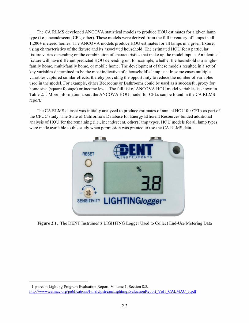
The CA RLMS developed ANCOVA statistical models to produce HOU estimates for a given lamp type (i.e., incandescent, CFL, other). These models were derived from the full inventory of lamps in all 1,200+ metered homes. The ANCOVA models produce HOU estimates for all lamps in a given fixture, using characteristics of the fixture and its associated household. The estimated HOU for a particular fixture varies depending on the combination of characteristics that make up the model inputs. An identical fixture will have different predicted HOU depending on, for example, whether the household is a single-family home, multi-family home, or mobile home. The development of these models resulted in a set of key variables determined to be the most indicative of a household’s lamp use. In some cases multiple variables captured similar effects, thereby providing the opportunity to reduce the number of variables used in the model. For example, either Bedrooms or Bathrooms could be used as a successful proxy for home size (square footage) or income level. The full list of ANCOVA HOU model variables is shown in Table 2.1. More information about the ANCOVA HOU model for CFLs can be found in the CA RLMS report.1

The CA RLMS dataset was initially analyzed to produce estimates of annual HOU for CFLs as part of the CPUC study. The State of California’s Database for Energy Efficient Resources funded additional analysis of HOU for the remaining (i.e., incandescent, other) lamp types. HOU models for all lamp types were made available to this study when permission was granted to use the CA RLMS data.

Figure 2.1. The DENT Instruments LIGHTING Logger Used to Collect End-Use Metering Data

1 Upstream Lighting Program Evaluation Report, Volume 1, Section 8.5. http://www.calmac.org/publications/FinalUpstreamLightingEvaluationReport_Vol1_CALMAC_3.pdf

2.2

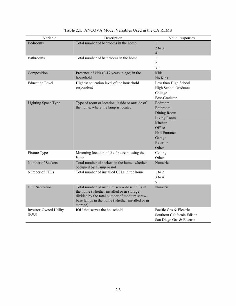
Table 2.1. ANCOVA Model Variables Used in the CA RLMS

Variable Description Valid Responses Bedrooms Total number of bedrooms in the home 1

2 to 3 4+

Bathrooms Total number of bathrooms in the home 1 2 3+

Composition Presence of kids (0-17 years in age) in the Kids household No Kids

Education Level Highest education level of the household Less than High School respondent High School Graduate

College Post-Graduate

Lighting Space Type Type of room or location, inside or outside of the home, where the lamp is located

Bedroom Bathroom Dining Room Living Room Kitchen Office Hall Entrance Garage Exterior Other

Fixture Type Mounting location of the fixture housing the lamp

Ceiling Other

Number of Sockets

Number of CFLs

Total number of sockets in the home, whether occupied by a lamp or not Total number of installed CFLs in the home

Numeric

1 to 2 3 to 4 5+

CFL Saturation Total number of medium screw-base CFLs in Numeric the home (whether installed or in storage) divided by the total number of medium screw-base lamps in the home (whether installed or in storage)

Investor-Owned Utility (IOU)

IOU that serves the household Pacific Gas & Electric Southern California Edison San Diego Gas & Electric

2.3

2.2 Residential Energy Consumption Survey

The EIA administers the RECS, which collects household characteristics and usage patterns from a nationally representative sample of housing units using specially trained interviewers. This information is combined with data from energy suppliers to these homes to estimate energy costs and usage for heating, cooling, appliances, and other end uses. The RECS was conducted yearly from 1978-1982, every third year from 1984-1993, and every fourth year thereafter. Various sets of RECS microdata are made publically available over time on the EIA website.

The estimation framework for this study is fundamentally based on the sample design for the 2009 RECS. The National Opinion Research Center collected onsite data for the 2009 RECS from February through August 2010. Although the previous 2005 RECS collected data from 4,382 households, the 2009 survey collected data from 12,083 households in housing units statistically selected to represent the 113.6 million housing units that are occupied as a primary residence. The large sample size and scope of the 2009 RECS make it an effort not likely to be repeated in the foreseeable future.

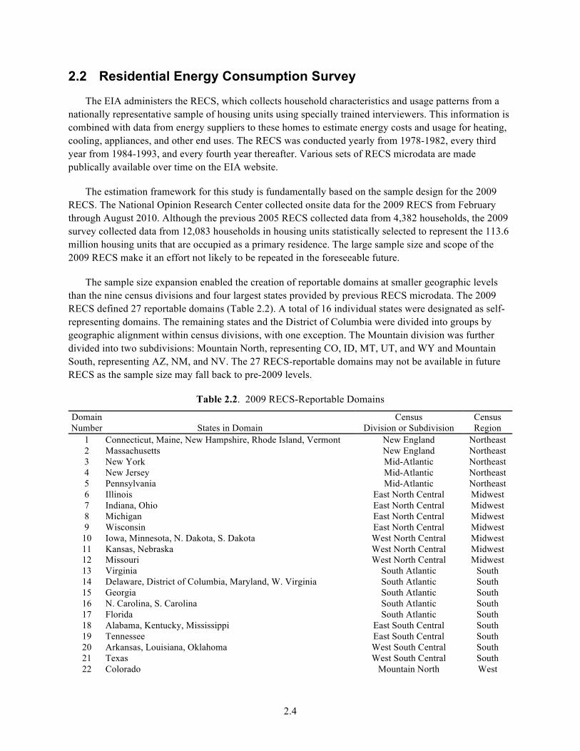
The sample size expansion enabled the creation of reportable domains at smaller geographic levels than the nine census divisions and four largest states provided by previous RECS microdata. The 2009 RECS defined 27 reportable domains (Table 2.2). A total of 16 individual states were designated as self-representing domains. The remaining states and the District of Columbia were divided into groups by geographic alignment within census divisions, with one exception. The Mountain division was further divided into two subdivisions: Mountain North, representing CO, ID, MT, UT, and WY and Mountain South, representing AZ, NM, and NV. The 27 RECS-reportable domains may not be available in future RECS as the sample size may fall back to pre-2009 levels.

Table 2.2. 2009 RECS-Reportable Domains

Domain Census Census Number States in Domain Division or Subdivision Region

1 Connecticut, Maine, New Hampshire, Rhode Island, Vermont New England Northeast 2 Massachusetts New England Northeast 3 New York Mid-Atlantic Northeast 4 New Jersey Mid-Atlantic Northeast 5 Pennsylvania Mid-Atlantic Northeast 6 Illinois East North Central Midwest 7 Indiana, Ohio East North Central Midwest 8 Michigan East North Central Midwest 9 Wisconsin East North Central Midwest

10 Iowa, Minnesota, N. Dakota, S. Dakota West North Central Midwest 11 Kansas, Nebraska West North Central Midwest 12 Missouri West North Central Midwest 13 Virginia South Atlantic South 14 Delaware, District of Columbia, Maryland, W. Virginia South Atlantic South 15 Georgia South Atlantic South 16 N. Carolina, S. Carolina South Atlantic South 17 Florida South Atlantic South 18 Alabama, Kentucky, Mississippi East South Central South 19 Tennessee East South Central South 20 Arkansas, Louisiana, Oklahoma West South Central South 21 Texas West South Central South 22 Colorado Mountain North West

2.4

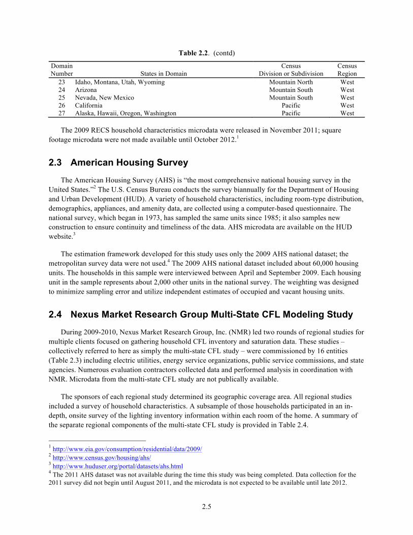
Table 2.2. (contd)

Domain Census Census Number States in Domain Division or Subdivision Region

23 Idaho, Montana, Utah, Wyoming Mountain North West 24 Arizona Mountain South West 25 Nevada, New Mexico Mountain South West 26 California Pacific West 27 Alaska, Hawaii, Oregon, Washington Pacific West

The 2009 RECS household characteristics microdata were released in November 2011; square footage microdata were not made available until October 2012.1

2.3 American Housing Survey

The American Housing Survey (AHS) is “the most comprehensive national housing survey in the United States.”2 The U.S. Census Bureau conducts the survey biannually for the Department of Housing and Urban Development (HUD). A variety of household characteristics, including room-type distribution, demographics, appliances, and amenity data, are collected using a computer-based questionnaire. The national survey, which began in 1973, has sampled the same units since 1985; it also samples new construction to ensure continuity and timeliness of the data. AHS microdata are available on the HUD website.3

The estimation framework developed for this study uses only the 2009 AHS national dataset; the metropolitan survey data were not used.4 The 2009 AHS national dataset included about 60,000 housing units. The households in this sample were interviewed between April and September 2009. Each housing unit in the sample represents about 2,000 other units in the national survey. The weighting was designed to minimize sampling error and utilize independent estimates of occupied and vacant housing units.

2.4 Nexus Market Research Group Multi-State CFL Modeling Study

During 2009-2010, Nexus Market Research Group, Inc. (NMR) led two rounds of regional studies for multiple clients focused on gathering household CFL inventory and saturation data. These studies – collectively referred to here as simply the multi-state CFL study – were commissioned by 16 entities (Table 2.3) including electric utilities, energy service organizations, public service commissions, and state agencies. Numerous evaluation contractors collected data and performed analysis in coordination with NMR. Microdata from the multi-state CFL study are not publically available.

The sponsors of each regional study determined its geographic coverage area. All regional studies included a survey of household characteristics. A subsample of those households participated in an in-depth, onsite survey of the lighting inventory information within each room of the home. A summary of the separate regional components of the multi-state CFL study is provided in Table 2.4.

1 http://www.eia.gov/consumption/residential/data/2009/ 2 http://www.census.gov/housing/ahs/3 http://www.huduser.org/portal/datasets/ahs.html 4 The 2011 AHS dataset was not available during the time this study was being completed. Data collection for the 2011 survey did not begin until August 2011, and the microdata is not expected to be available until late 2012.

2.5

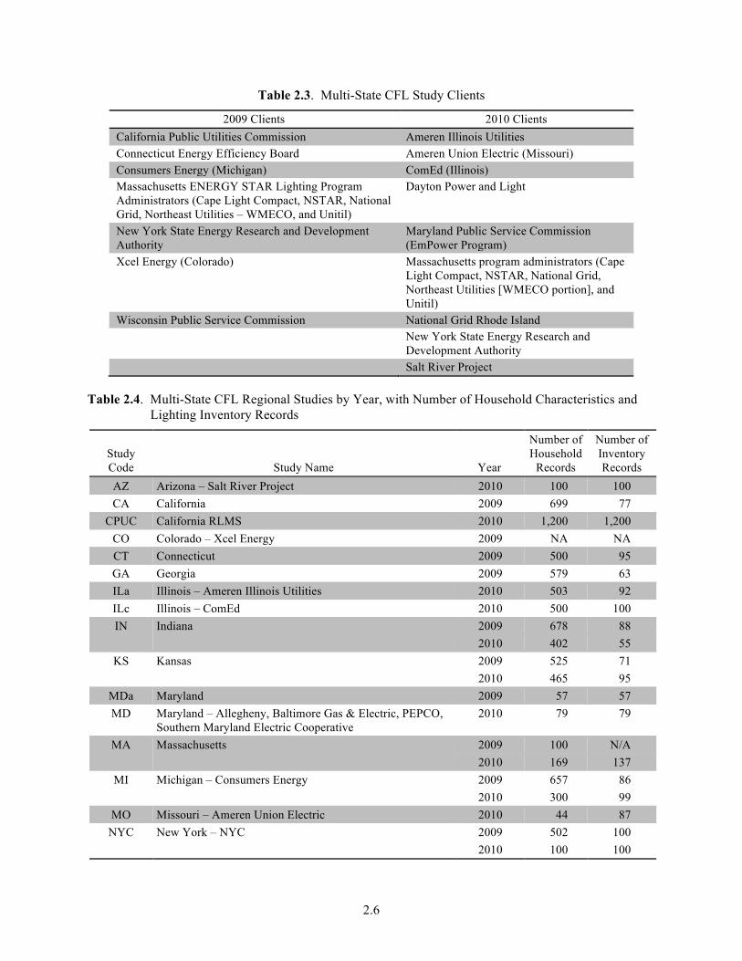
Table 2.3. Multi-State CFL Study Clients

2009 Clients 2010 Clients California Public Utilities Commission Ameren Illinois Utilities Connecticut Energy Efficiency Board Ameren Union Electric (Missouri) Consumers Energy (Michigan) ComEd (Illinois) Massachusetts ENERGY STAR Lighting Program Dayton Power and Light Administrators (Cape Light Compact, NSTAR, National Grid, Northeast Utilities – WMECO, and Unitil) New York State Energy Research and Development Maryland Public Service Commission Authority (EmPower Program) Xcel Energy (Colorado) Massachusetts program administrators (Cape

Light Compact, NSTAR, National Grid, Northeast Utilities [WMECO portion], and Unitil)

Wisconsin Public Service Commission National Grid Rhode Island New York State Energy Research and Development Authority Salt River Project

Table 2.4. Multi-State CFL Regional Studies by Year, with Number of Household Characteristics and Lighting Inventory Records

Number of Number of Study Household Inventory Code Study Name Year Records Records AZ Arizona – Salt River Project 2010 100 100 CA California 2009 699 77

CPUC California RLMS 2010 1,200 1,200 CO Colorado – Xcel Energy 2009 NA NA CT Connecticut 2009 500 95 GA Georgia 2009 579 63 ILa Illinois – Ameren Illinois Utilities 2010 503 92 ILc Illinois – ComEd 2010 500 100 IN Indiana 2009 678 88

2010 402 55 KS Kansas 2009 525 71

2010 465 95 MDa Maryland 2009 57 57 MD Maryland – Allegheny, Baltimore Gas & Electric, PEPCO, 2010 79 79

Southern Maryland Electric Cooperative MA Massachusetts 2009 100 N/A

2010 169 137 MI Michigan – Consumers Energy 2009 657 86

2010 300 99 MO Missouri – Ameren Union Electric 2010 44 87

NYC New York – NYC 2009 502 100 2010 100 100

2.6

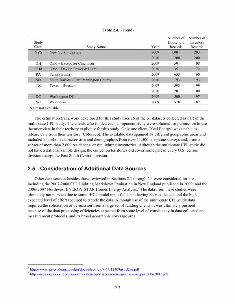
Table 2.4. (contd)

Number of Number of Study Household Inventory Code Study Name Year Records Records NYS New York – Upstate 2009 1,001 203

2010 200 200 OH Ohio – Except for Cincinnati 2009 501 98

OHd Ohio – Dayton Power & Light 2010 351 72 PA Pennsylvania 2009 653 60 SD South Dakota – Part Pennington County 2010 93 93 TX Texas – Houston 2009 503 99

2010 201 100 DC Washington DC 2009 500 97 WI Wisconsin 2009 578 82

NA = not available

The estimation framework developed for this study uses 26 of the 31 datasets collected as part of the multi-state CFL study. The clients who funded each component study were solicited for permission to use the microdata in their territory explicitly for this study. Only one client (Xcel Energy) was unable to release data from their territory (Colorado). The available data spanned 18 different geographic areas and included household characteristics and demographics from over 11,500 telephone surveys and, from a subset of more than 2,600 residences, onsite lighting inventories. Although the multi-state CFL study did not have a national sample design, the collection territories did cover some part of every U.S. census division except the East South Central division.

2.5 Consideration of Additional Data Sources

Other data sources besides those reviewed in Sections 2.1 through 2.4 were considered for use, including the 2007-2008 CFL Lighting Markdown Evaluation in New England published in 20091 and the 2006-2007 Northwest ENERGY STAR Homes Energy Analysis.2 The data from these studies were ultimately not pursued due to some HOU model input fields not having been collected, and the high expected level of effort required to recode the data. Although use of the multi-state CFL study data required the solicitation of permission from a large set of funding clients, it was ultimately pursued because of the data processing efficiencies expected from some level of consistency in data collected and measurement protocols, and its broad geographic coverage area.

1 http://www.env.state.ma.us/dpu/docs/electric/09-64/12409nstrd2ae.pdf 2 http://neea.org/docs/reports/northwestenergystarhomesenergyanalysisreport20062007.pdf

2.7

3.0 Methodology

The national and regional estimates of lighting usage produced in this study are based on the outputs of the HOU models developed from the CA RLMS dataset, as described in Section 2.1. These models were leveraged here to take advantage of the unique qualities of this dataset, including its broad scope (i.e., coverage of residence types, room types, and lamp types), large sample size, and uniform collection methodology. Reuse of these models requires input data that meet defined pre-conditions – specifically that the data contain the variables used by the ANCOVA models, or variables that can be recoded to those used by the ANCOVA models. It was possible to use the ANCOVA HOU models in this study because the model inputs defined by the CA RLMS were available collectively in the selected data sources. While not all inputs were available in each data source, methods for creating linkages between the datasets were identified that allowed for a combination of the RECS, the AHS, and the multi-state CFL study data (combined with the CA RLMS data) to generate regionally representative inputs for the ANCOVA HOU models.

The HOU models were thus applied to regionally varying input data, referred to here as the estimation framework, rather than only California households. The estimation framework is the 2009 RECS sample, expanded by imputing additional measures for each housing unit in the sample using data from other sources. These extensions were made by linking fields in multiple datasets containing national and regional information with equivalent fields used as inputs to the HOU models. After creating these linkages, relevant data from each data source were extracted, resulting in a composite dataset of housing units described by all of the inputs needed by the HOU models, and statistically representative of the entire United States and its sub-regions. The following sections describe the creation of this estimation framework in more detail, as well as the methods used to apply the HOU models to the estimation framework, generate lamp-level usage and energy consumption estimates, and aggregate those and other estimates to various levels.

3.1 Estimation Framework Characteristics

Each housing unit in the estimation framework is described by its household characteristics, lighting spaces, and lighting inventory. The following sections describe the variables collected for each of these categories, including parent datasets, valid variable values, and application in this study. Valid values for variables used by the HOU models were established to be consistent with those used in the CA RLMS.

3.1.1 Household Characteristic Variables

Household characteristics include housing unit characteristics, occupant demographics, and lighting/room space types. Housing unit characteristic and occupant demographic data are available with consistent definitions and in consistent formats from the RECS, AHS, multi-state CFL study, and CA RLMS datasets, making these variables useful for linking the datasets together for the purpose of assigning data from one dataset to housing unit samples of another. The lamp HOU models use four of the seven housing unit and occupant demographic variables in the estimation framework, summarized in Table 3.1 and Table 3.2, respectively. Estimates were generated in this study at every valid value level for all household characteristic variables, with the exception of the Rooms variable.

3.1

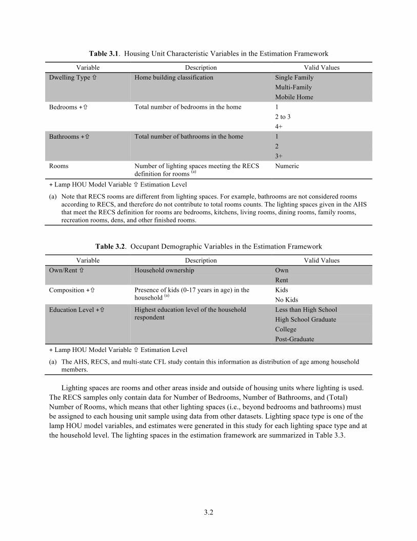
Table 3.1. Housing Unit Characteristic Variables in the Estimation Framework

Variable Description Valid Values Dwelling Type!! Home building classification Single Family

Multi-Family Mobile Home

Bedrooms +! Total number of bedrooms in the home 1 2 to 3 4+

Bathrooms +! Total number of bathrooms in the home 1 2 3+

Rooms Number of lighting spaces meeting the RECS Numeric definition for rooms (a)

+!Lamp HOU Model Variable !!Estimation Level

(a) Note that RECS rooms are different from lighting spaces. For example, bathrooms are not considered rooms according to RECS, and therefore do not contribute to total rooms counts. The lighting spaces given in the AHS that meet the RECS definition for rooms are bedrooms, kitchens, living rooms, dining rooms, family rooms, recreation rooms, dens, and other finished rooms.

Table 3.2. Occupant Demographic Variables in the Estimation Framework

Variable Description Valid Values Own/Rent ! Household ownership Own

Rent Composition +! Presence of kids (0-17 years in age) in the Kids

household (a) No Kids

Education Level +! Highest education level of the household respondent

Less than High School High School Graduate College Post-Graduate

+ Lamp HOU Model Variable ! Estimation Level

(a) The AHS, RECS, and multi-state CFL study contain this information as distribution of age among household members.

Lighting spaces are rooms and other areas inside and outside of housing units where lighting is used. The RECS samples only contain data for Number of Bedrooms, Number of Bathrooms, and (Total) Number of Rooms, which means that other lighting spaces (i.e., beyond bedrooms and bathrooms) must be assigned to each housing unit sample using data from other datasets. Lighting space type is one of the lamp HOU model variables, and estimates were generated in this study for each lighting space type and at the household level. The lighting spaces in the estimation framework are summarized in Table 3.3.

3.2

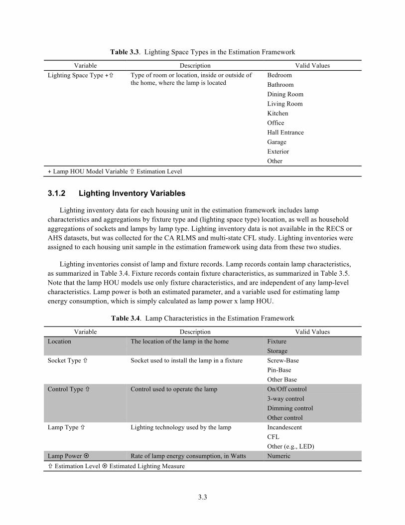
Table 3.3. Lighting Space Types in the Estimation Framework

Variable Description Valid Values Lighting Space Type +! Type of room or location, inside or outside of

the home, where the lamp is located Bedroom Bathroom Dining Room Living Room Kitchen Office Hall Entrance Garage Exterior Other

+ Lamp HOU Model Variable ! Estimation Level

3.1.2 Lighting Inventory Variables

Lighting inventory data for each housing unit in the estimation framework includes lamp characteristics and aggregations by fixture type and (lighting space type) location, as well as household aggregations of sockets and lamps by lamp type. Lighting inventory data is not available in the RECS or AHS datasets, but was collected for the CA RLMS and multi-state CFL study. Lighting inventories were assigned to each housing unit sample in the estimation framework using data from these two studies.

Lighting inventories consist of lamp and fixture records. Lamp records contain lamp characteristics, as summarized in Table 3.4. Fixture records contain fixture characteristics, as summarized in Table 3.5. Note that the lamp HOU models use only fixture characteristics, and are independent of any lamp-level characteristics. Lamp power is both an estimated parameter, and a variable used for estimating lamp energy consumption, which is simply calculated as lamp power x lamp HOU.

Table 3.4. Lamp Characteristics in the Estimation Framework

Variable Description Valid Values Location The location of the lamp in the home Fixture

Storage Socket Type ! Socket used to install the lamp in a fixture Screw-Base

Pin-Base Other Base

Control Type ! Control used to operate the lamp On/Off control 3-way control Dimming control Other control

Lamp Type ! Lighting technology used by the lamp Incandescent CFL Other (e.g., LED)

Lamp Power " Rate of lamp energy consumption, in Watts Numeric ! Estimation Level " Estimated Lighting Measure

3.3

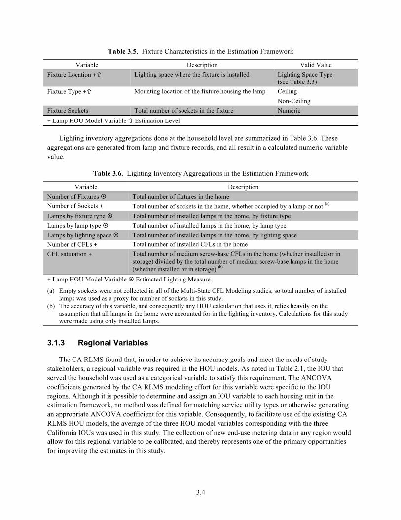
Table 3.5. Fixture Characteristics in the Estimation Framework

Variable Description Valid Value Fixture Location +! Lighting space where the fixture is installed Lighting Space Type

(see Table 3.3) Fixture Type +! Mounting location of the fixture housing the lamp Ceiling

Non-Ceiling Fixture Sockets Total number of sockets in the fixture Numeric +!Lamp HOU Model Variable !!Estimation Level

Lighting inventory aggregations done at the household level are summarized in Table 3.6. These aggregations are generated from lamp and fixture records, and all result in a calculated numeric variable value.

Table 3.6. Lighting Inventory Aggregations in the Estimation Framework

Variable Description Number of Fixtures " Total number of fixtures in the home Number of Sockets + Total number of sockets in the home, whether occupied by a lamp or not (a)

Lamps by fixture type " Total number of installed lamps in the home, by fixture type Lamps by lamp type " Total number of installed lamps in the home, by lamp type Lamps by lighting space " Total number of installed lamps in the home, by lighting space Number of CFLs + Total number of installed CFLs in the home CFL saturation + Total number of medium screw-base CFLs in the home (whether installed or in

storage) divided by the total number of medium screw-base lamps in the home (whether installed or in storage) (b)

+ Lamp HOU Model Variable " Estimated Lighting Measure

(a) Empty sockets were not collected in all of the Multi-State CFL Modeling studies, so total number of installed lamps was used as a proxy for number of sockets in this study.

(b) The accuracy of this variable, and consequently any HOU calculation that uses it, relies heavily on the assumption that all lamps in the home were accounted for in the lighting inventory. Calculations for this study were made using only installed lamps.

3.1.3 Regional Variables

The CA RLMS found that, in order to achieve its accuracy goals and meet the needs of study stakeholders, a regional variable was required in the HOU models. As noted in Table 2.1, the IOU that served the household was used as a categorical variable to satisfy this requirement. The ANCOVA coefficients generated by the CA RLMS modeling effort for this variable were specific to the IOU regions. Although it is possible to determine and assign an IOU variable to each housing unit in the estimation framework, no method was defined for matching service utility types or otherwise generating an appropriate ANCOVA coefficient for this variable. Consequently, to facilitate use of the existing CA RLMS HOU models, the average of the three HOU model variables corresponding with the three California IOUs was used in this study. The collection of new end-use metering data in any region would allow for this regional variable to be calibrated, and thereby represents one of the primary opportunities for improving the estimates in this study.

3.4

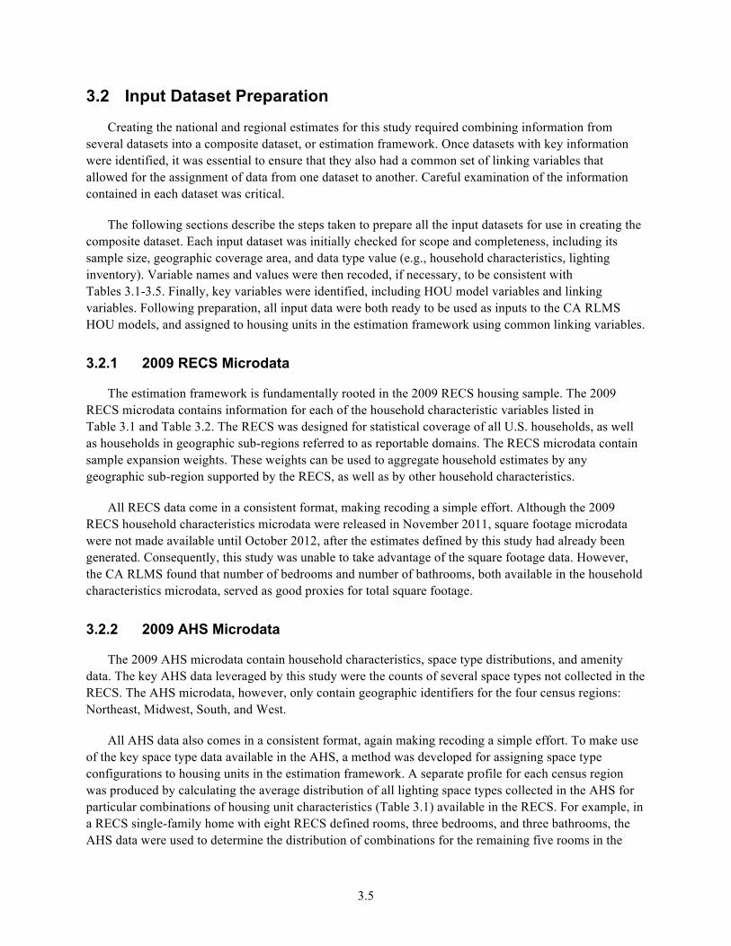
3.2 Input Dataset Preparation

Creating the national and regional estimates for this study required combining information from several datasets into a composite dataset, or estimation framework. Once datasets with key information were identified, it was essential to ensure that they also had a common set of linking variables that allowed for the assignment of data from one dataset to another. Careful examination of the information contained in each dataset was critical.

The following sections describe the steps taken to prepare all the input datasets for use in creating the composite dataset. Each input dataset was initially checked for scope and completeness, including its sample size, geographic coverage area, and data type value (e.g., household characteristics, lighting inventory). Variable names and values were then recoded, if necessary, to be consistent with Tables 3.1-3.5. Finally, key variables were identified, including HOU model variables and linking variables. Following preparation, all input data were both ready to be used as inputs to the CA RLMS HOU models, and assigned to housing units in the estimation framework using common linking variables.

3.2.1 2009 RECS Microdata

The estimation framework is fundamentally rooted in the 2009 RECS housing sample. The 2009 RECS microdata contains information for each of the household characteristic variables listed in Table 3.1 and Table 3.2. The RECS was designed for statistical coverage of all U.S. households, as well as households in geographic sub-regions referred to as reportable domains. The RECS microdata contain sample expansion weights. These weights can be used to aggregate household estimates by any geographic sub-region supported by the RECS, as well as by other household characteristics.

All RECS data come in a consistent format, making recoding a simple effort. Although the 2009 RECS household characteristics microdata were released in November 2011, square footage microdata were not made available until October 2012, after the estimates defined by this study had already been generated. Consequently, this study was unable to take advantage of the square footage data. However, the CA RLMS found that number of bedrooms and number of bathrooms, both available in the household characteristics microdata, served as good proxies for total square footage.

3.2.2 2009 AHS Microdata

The 2009 AHS microdata contain household characteristics, space type distributions, and amenity data. The key AHS data leveraged by this study were the counts of several space types not collected in the RECS. The AHS microdata, however, only contain geographic identifiers for the four census regions: Northeast, Midwest, South, and West.

All AHS data also comes in a consistent format, again making recoding a simple effort. To make use of the key space type data available in the AHS, a method was developed for assigning space type configurations to housing units in the estimation framework. A separate profile for each census region was produced by calculating the average distribution of all lighting space types collected in the AHS for particular combinations of housing unit characteristics (Table 3.1) available in the RECS. For example, in a RECS single-family home with eight RECS defined rooms, three bedrooms, and three bathrooms, the AHS data were used to determine the distribution of combinations for the remaining five rooms in the

3.5

home (other than the three bedrooms) and other space types where lighting is used (including bathrooms) that do not meet the RECS definition for a room. The housing unit characteristics chosen as linking variables were selected for two reasons. First, they provide information about the physical structure of the home. Second, they strike a balance between matching by too few variables, in which case the matched AHS households could have very little in common with the RECS households that they were being matched to, and too many variables, which could lead to valid household matches being excluded.

3.2.3 2009-2010 Multi-State CFL Study Microdata

The 2009-2010 multi-state CFL study microdata contain household characteristics and, most importantly, lighting inventory data by lighting space type. The lighting inventory data were used to regionally assign fixtures and lamps to housing units in the estimation framework with lighting space distributions assigned by the AHS data.

Although the two rounds of regional studies that comprised the multi-state CFL study had a common goal and management, numerous evaluation contractors collected and processed the data. As a result, additional effort was required to process, recode, and make use of the 30 separate datasets made available to this study. The following sections explain some of the methods employed to prepare the multi-state CFL study data.

3.2.3.1 Linking Household and Lighting Inventory Data

Each regional study in the multi-state CFL study provided two datasets – a household characteristics dataset and a lighting inventory dataset. The inventory dataset was typically a subset of the characteristics dataset. The first step in preparing the multi-state CFL data was to verify that housing units in both datasets could be matched, usually with a case identification number. All inventory dataset housing units were successfully linked to a characteristics dataset housing unit, with the exception of four units in the 2010 Illinois – ComEd study and one unit in the 2010 Massachusetts study. The Massachusetts study had two characteristics datasets and two inventory datasets, one of each for 2009 and one of each for 2010. The 2010 datasets included a matching variable, but the 2009 datasets did not, resulting in the exclusion of the 2009 Massachusetts data.

3.2.3.2 Recoding Variables

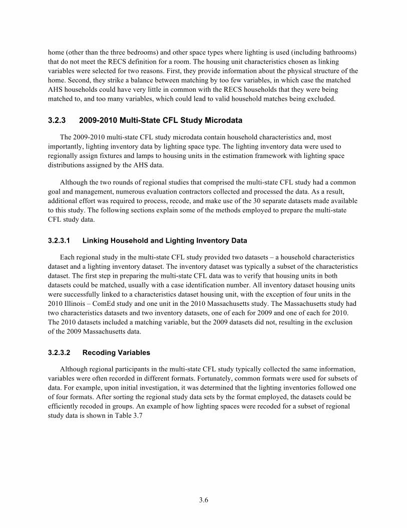
Although regional participants in the multi-state CFL study typically collected the same information, variables were often recorded in different formats. Fortunately, common formats were used for subsets of data. For example, upon initial investigation, it was determined that the lighting inventories followed one of four formats. After sorting the regional study data sets by the format employed, the datasets could be efficiently recoded in groups. An example of how lighting spaces were recoded for a subset of regional study data is shown in Table 3.7

3.6

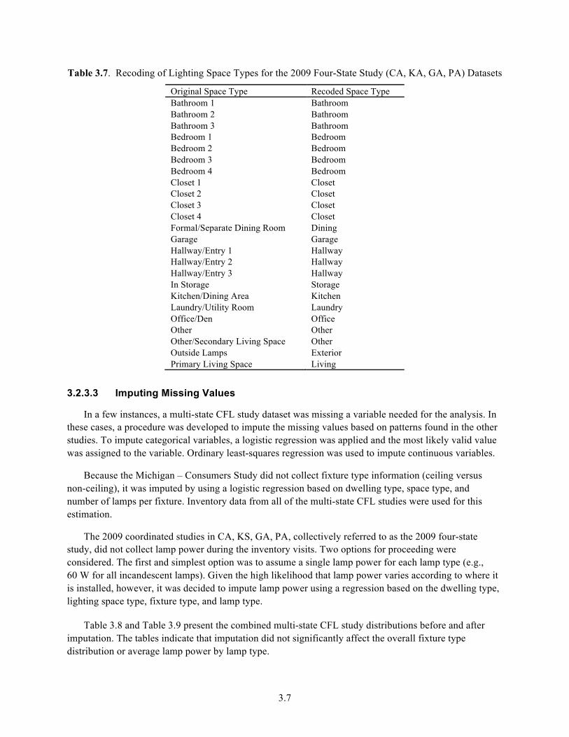
Table 3.7. Recoding of Lighting Space Types for the 2009 Four-State Study (CA, KA, GA, PA) Datasets

Original Space Type Recoded Space Type Bathroom 1 Bathroom Bathroom 2 Bathroom Bathroom 3 Bathroom Bedroom 1 Bedroom Bedroom 2 Bedroom Bedroom 3 Bedroom Bedroom 4 Bedroom Closet 1 Closet Closet 2 Closet Closet 3 Closet Closet 4 Closet Formal/Separate Dining Room Dining Garage Garage Hallway/Entry 1 Hallway Hallway/Entry 2 Hallway Hallway/Entry 3 Hallway In Storage Storage Kitchen/Dining Area Kitchen Laundry/Utility Room Laundry Office/Den Office Other Other Other/Secondary Living Space Other Outside Lamps Exterior Primary Living Space Living

3.2.3.3 Imputing Missing Values

In a few instances, a multi-state CFL study dataset was missing a variable needed for the analysis. In these cases, a procedure was developed to impute the missing values based on patterns found in the other studies. To impute categorical variables, a logistic regression was applied and the most likely valid value was assigned to the variable. Ordinary least-squares regression was used to impute continuous variables.

Because the Michigan – Consumers Study did not collect fixture type information (ceiling versus non-ceiling), it was imputed by using a logistic regression based on dwelling type, space type, and number of lamps per fixture. Inventory data from all of the multi-state CFL studies were used for this estimation.

The 2009 coordinated studies in CA, KS, GA, PA, collectively referred to as the 2009 four-state study, did not collect lamp power during the inventory visits. Two options for proceeding were considered. The first and simplest option was to assume a single lamp power for each lamp type (e.g., 60 W for all incandescent lamps). Given the high likelihood that lamp power varies according to where it is installed, however, it was decided to impute lamp power using a regression based on the dwelling type, lighting space type, fixture type, and lamp type.

Table 3.8 and Table 3.9 present the combined multi-state CFL study distributions before and after imputation. The tables indicate that imputation did not significantly affect the overall fixture type distribution or average lamp power by lamp type.

3.7

Table 3.8. Fixture Type Distribution, Before and After Imputation in Michigan – Consumers Study Territory

Multi-State CFL Multi-State CFL Study After Study Before Imputation in Michigan – Michigan – Consumers

Fixture Type Imputation Consumers Territory Territory After Imputation Ceiling 55.2% 55.4% 59.8% Other 44.9% 44.6% 40.2%

Table 3.9. Average Lamp Power (W) by Lamp Type, Before and After Imputation in 2009 Four-State Study Territories

Multi-State CFL Study Multi-State CFL Study After Imputation in 2009 Four-State Study

Before Imputation 2009 Four-State Study After Imputation CFL 16.7 16.4 15.8 Incandescent 61.4 61.8 62.4 Other 46.6 52.2 59.9

3.2.3.4 2009 Four-State Study Data (CA, KS, GA, PA)

Following the data examination process, it was determined that the 2009 four-state study could not be used for estimating HOU for a number of reasons. First, the four-state study collected lighting information only at the room level, not at the fixture level as the CA RLMS and the other multi-state CFL studies had done. Second, the four-state study only recorded counts of CFLs and total number of lamps, without distinguishing incandescent and other lamp types. Finally, the four-state study did not record socket types.

Although the missing data could have been imputed by leveraging other sources, little information would be gained by doing so. Usable information from the four-state study (i.e., demographics and space type) was also available from the RECS and AHS. Furthermore, a reconstructed dataset would not be significantly different from an average of the other studies.

3.3 Combining Datasets

The RECS, AHS, and multi-state CFL study datasets were combined to create a composite dataset, or estimation framework, from which all lighting estimates were generated. More specifically, the data representing each RECS case was extended with data from each of the other two sources so that each RECS case could be described using all the variables in the ANCOVA model.

3.3.1 Extending RECS Housing Units with AHS Data

RECS housing units were extended with AHS data to augment the lighting space information in the RECS case. The RECS only collects number of bedrooms, number of bathrooms, and number of other rooms, but the AHS provides data on more specific lighting space types. Although the RECS provides sample units for 27 domains, each AHS household is only categorized by 1 of 4 census regions. Census region was therefore used as the geographic variable linking the RECS and the AHS datasets.

Lighting space configurations are possible combinations of lighting space types for a housing unit. Lighting space configurations from the AHS were assigned to RECS cases using a total of five linking

3.8

variables: census region, dwelling type, number of bedrooms, number of bathrooms, and total number of rooms in the household.1 Because the AHS microdata include many more sample cases than the RECS, and the AHS geographic identifiers are at a higher level than those of the RECS, multiple space type configurations are generally linked to each RECS case. Rather than choosing a single AHS space type configuration to match to each RECS case, a separate RECS replicate housing unit was created for each of the multiple configurations for analysis. The AHS weight was used to give the level of contribution to each configuration.

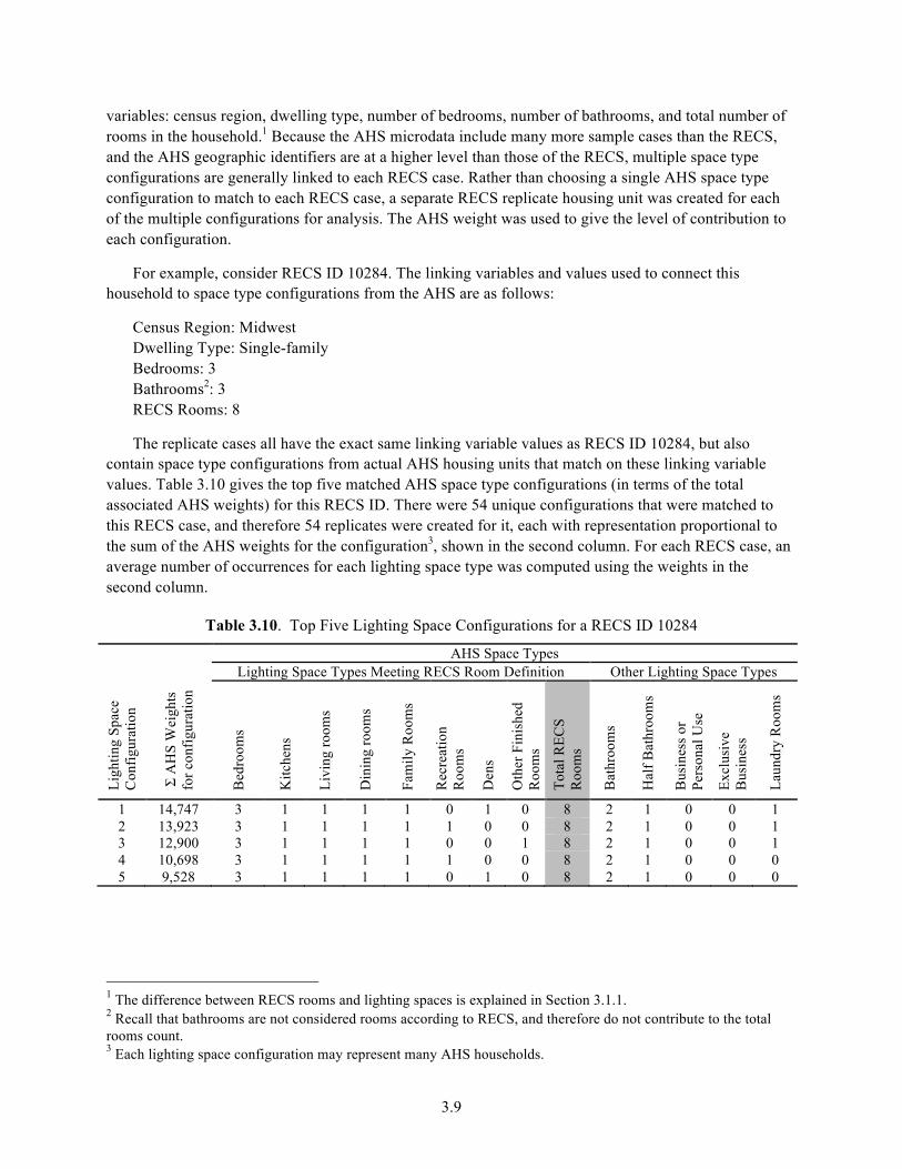
For example, consider RECS ID 10284. The linking variables and values used to connect this household to space type configurations from the AHS are as follows:

Census Region: Midwest Dwelling Type: Single-family Bedrooms: 3 Bathrooms2: 3 RECS Rooms: 8

The replicate cases all have the exact same linking variable values as RECS ID 10284, but also contain space type configurations from actual AHS housing units that match on these linking variable values. Table 3.10 gives the top five matched AHS space type configurations (in terms of the total associated AHS weights) for this RECS ID. There were 54 unique configurations that were matched to this RECS case, and therefore 54 replicates were created for it, each with representation proportional to the sum of the AHS weights for the configuration3, shown in the second column. For each RECS case, an average number of occurrences for each lighting space type was computed using the weights in the second column.

Table 3.10. Top Five Lighting Space Configurations for a RECS ID 10284

AHS Space Types Lighting Space Types Meeting RECS Room Definition Other Lighting Space Types

Ligh

ting

Spac

eC

onfig

urat

ion

Σ A

HS

Wei

ghts

for c

onfig

urat

ion

Bed

room

s

Kitc

hens

Livi

ng ro

oms

Din

ing

room

s

Fam

ily R

oom

s

Rec

reat

ion

Roo

ms

Den

s

Oth

er F

inis

hed

Roo

ms

Tota

l REC

SR

oom

s

Bat

hroo

ms

Hal

f Bat

hroo

ms

Bus

ines

s or

Pers

onal

Use

Excl

usiv

eB

usin

ess

Laun

dry

Roo

ms

1 14,747 3 1 1 1 1 0 1 0 8 2 1 0 0 1 2 13,923 3 1 1 1 1 1 0 0 8 2 1 0 0 1 3 12,900 3 1 1 1 1 0 0 1 8 2 1 0 0 1 4 10,698 3 1 1 1 1 1 0 0 8 2 1 0 0 0 5 9,528 3 1 1 1 1 0 1 0 8 2 1 0 0 0

1 The difference between RECS rooms and lighting spaces is explained in Section 3.1.1. 2 Recall that bathrooms are not considered rooms according to RECS, and therefore do not contribute to the total rooms count. 3 Each lighting space configuration may represent many AHS households.

3.9

Out of 12,083 households in the 2009 RECS, only 178 (or 1.5 percent) could not be matched to any AHS configuration using this approach. These cases were discarded from the analysis, and the weights for the remaining RECS cases were adjusted so that the sum of the weights before and after the drop was the same.

3.3.2 Extending RECS Housing Units with Multi-State CFL Study Data

The next step in the creation of the estimation framework was to combine the newly formed RECS-AHS housing unit samples with the multi-state CFL study data. The RECS housing units were further extended with lighting configurations (consisting of fixtures and lamps) based on the multi-state CFL study lighting inventory data.

Whereas the RECS and AHS datasets covered all U.S. census divisions, the multi-state CFL study datasets had limited and specific coverage areas. Furthermore, the distribution and sample size for each coverage area varied. To overcome these limitations, each RECS domain was assigned one or more individual multi-state CFL study dataset based on geographic proximity. These datasets were weighted to indicate how much each one should be represented when aggregated to the RECS domain level. For locations where no regional study was reasonably close, a combination of the entire multi-state CFL study was used.

Following the development of a strategy for combining individual multi-state CFL studies to represent each RECS domain, a number of methods for combining these datasets with the RECS-AHS data were investigated. An iterative procedure was developed. First, two primary linking variables were selected that were mandatory for matching: dwelling type and lighting space type. For example, the procedure would not match lighting configuration from a multi-family household into a single-family household, nor would it match lighting configurations from a garage into a bedroom. Then, a secondary list of linking variables was chosen that would be used for matching when possible: own/rent, composition, education level, bedrooms, and bathrooms.

The lighting configurations assigned from the multi-state CFL study lighting inventory data included lamp characteristics (socket type, control type, lamp type, lamp power), fixture characteristics (fixture type, fixture sockets), and aggregations including total number of fixtures and lamps. The iterative process for matching and making assignments began with a list of secondary linking variables to match. In the first iteration, all secondary variables were included. In subsequent iterations, the list was reduced by a single variable to increase the chances of matching. Lighting inventory data with matching variables (primary and secondary) were aggregated across the component studies assigned to each RECS domain, weighted, and assigned. This process was repeated until each RECS housing unit had been extended with a lighting configuration. This process took up to 23 iterations for each RECS domain.

Because the multi-state CFL study included limited data for mobile homes, all the mobile homes were pooled into a single dataset to be used for all domains.

3.3.3 Estimation Framework Summary

Table 3.11 summarizes the different sources of information that were used for each state, including how the 2009-2010 multi-state CFL study datasets were assigned. Each state belongs to one of the 27

3.10

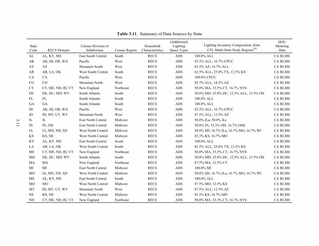
Table 3.11. Summary of Data Sources by State

3.11

State Code RECS Domain

Census Division or Subdivision Census Region

Household Characteristics

(Additional) Lighting

Space Types Lighting Inventory Composition, from

CFL Multi-State Study Regions(a)

HOU Metering

Data AL AL, KY, MS East South Central South RECS AHS 100.0% ALL CA RLMS AK AK, HI, OR, WA Pacific West RECS AHS 83.3% ALL, 16.7% CPUC CA RLMS AZ AZ Mountain South West RECS AHS 83.3% AZ, 16.7% ALL CA RLMS AR AR, LA, OK West South Central South RECS AHS 62.5% ALL, 25.0% TX, 12.5% KS CA RLMS CA CA Pacific West RECS AHS 100.0% CPUC CA RLMS CO CO Mountain North West RECS AHS 85.7% ALL, 14.3% AZ CA RLMS CT CT, ME, NH, RI, VT New England Northeast RECS AHS 50.0% MA, 33.3% CT, 16.7% NYS CA RLMS DE DE, DC, MD, WV South Atlantic South RECS AHS 50.0% MD, 25.0% DC, 12.5% ALL, 12.5% OH CA RLMS FL FL South Atlantic South RECS AHS 100.0% ALL CA RLMS GA GA South Atlantic South RECS AHS 100.0% ALL CA RLMS HI AK, HI, OR, WA Pacific West RECS AHS 83.3% ALL, 16.7% CPUC CA RLMS ID ID, MT, UT, WY Mountain North West RECS AHS 87.5% ALL, 12.5% AZ CA RLMS IL IL East North Central Midwest RECS AHS 50.0% ILa, 50.0% ILc CA RLMS IN IN, OH East North Central Midwest RECS AHS 50.0% IN, 33.3% OH, 16.7% OHd CA RLMS IA IA, MN, ND, SD West North Central Midwest RECS AHS 50.0% SD, 16.7% ILa, 16.7% MO, 16.7% WI CA RLMS KS KS, NE West North Central Midwest RECS AHS 83.3% KS, 16.7% MO CA RLMS KY AL, KY, MS East South Central South RECS AHS 100.0% ALL CA RLMS LA AR, LA, OK West South Central South RECS AHS 62.5% ALL, 25.0% TX, 12.5% KS CA RLMS ME CT, ME, NH, RI, VT New England Northeast RECS AHS 50.0% MA, 33.3% CT, 16.7% NYS CA RLMS MD DE, DC, MD, WV South Atlantic South RECS AHS 50.0% MD, 25.0% DC, 12.5% ALL, 12.5% OH CA RLMS MA MA New England Northeast RECS AHS 87.5% MA, 12.5% CT CA RLMS MI MI East North Central Midwest RECS AHS 100.0% MI CA RLMS MN IA, MN, ND, SD West North Central Midwest RECS AHS 50.0% SD, 16.7% ILa, 16.7% MO, 16.7% WI CA RLMS MS AL, KY, MS East South Central South RECS AHS 100.0% ALL CA RLMS MO MO West North Central Midwest RECS AHS 87.5% MO, 12.5% KS CA RLMS MT ID, MT, UT, WY Mountain North West RECS AHS 87.5% ALL, 12.5% AZ CA RLMS NE KS, NE West North Central Midwest RECS AHS 83.3% KS, 16.7% MO CA RLMS NH CT, ME, NH, RI, VT New England Northeast RECS AHS 50.0% MA, 33.3% CT, 16.7% NYS CA RLMS

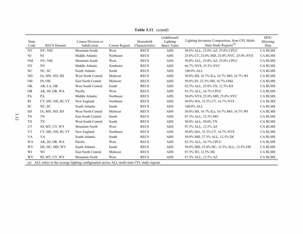
Table 3.11. (contd)

3.12

State Code RECS Domain

Census Division or Subdivision Census Region

Household Characteristics

(Additional) Lighting

Space Types Lighting Inventory Composition, from CFL Multi-

State Study Regions(a)

HOU Metering

Data NV NV, NM Mountain South West RECS AHS 50.0% ALL, 25.0% AZ, 25.0% CPUC CA RLMS NJ NJ Middle Atlantic Northeast RECS AHS 25.0% CT, 25.0% MD, 25.0% NYC, 25.0% NYS CA RLMS NM NV, NM Mountain South West RECS AHS 50.0% ALL, 25.0% AZ, 25.0% CPUC CA RLMS NY NY Middle Atlantic Northeast RECS AHS 66.7% NYS, 33.3% NYC CA RLMS NC NC, SC South Atlantic South RECS AHS 100.0% ALL CA RLMS ND IA, MN, ND, SD West North Central Midwest RECS AHS 50.0% SD, 16.7% ILa, 16.7% MO, 16.7% WI CA RLMS OH IN, OH East North Central Midwest RECS AHS 50.0% IN, 33.3% OH, 16.7% OHd CA RLMS OK AR, LA, OK West South Central South RECS AHS 62.5% ALL, 25.0% TX, 12.5% KS CA RLMS OR AK, HI, OR, WA Pacific West RECS AHS 83.3% ALL, 16.7% CPUC CA RLMS PA PA Middle Atlantic Northeast RECS AHS 50.0% NYS, 25.0% MD, 25.0% NYC CA RLMS RI CT, ME, NH, RI, VT New England Northeast RECS AHS 50.0% MA, 33.3% CT, 16.7% NYS CA RLMS SC NC, SC South Atlantic South RECS AHS 100.0% ALL CA RLMS SD IA, MN, ND, SD West North Central Midwest RECS AHS 50.0% SD, 16.7% ILa, 16.7% MO, 16.7% WI CA RLMS TN TN East South Central South RECS AHS 87.5% ALL, 12.5% MO CA RLMS TX TX West South Central South RECS AHS 50.0% ALL, 50.0% TX CA RLMS UT ID, MT, UT, WY Mountain North West RECS AHS 87.5% ALL, 12.5% AZ CA RLMS VT CT, ME, NH, RI, VT New England Northeast RECS AHS 50.0% MA, 33.3% CT, 16.7% NYS CA RLMS VA VA South Atlantic South RECS AHS 50.0% MD, 37.5% ALL, 12.5% DC CA RLMS WA AK, HI, OR, WA Pacific West RECS AHS 83.3% ALL, 16.7% CPUC CA RLMS WV DE, DC, MD, WV South Atlantic South RECS AHS 50.0% MD, 25.0% DC, 12.5% ALL, 12.5% OH CA RLMS WI WI East North Central Midwest RECS AHS 87.5% WI, 12.5% MI CA RLMS WY ID, MT, UT, WY Mountain North West RECS AHS 87.5% ALL, 12.5% AZ CA RLMS (a) ALL refers to the average lighting configuration across ALL multi-state CFL study regions

RECS domains. Household characteristics came from the 2009 RECS, with additional lighting spaces drawn from the 2009 AHS. End-use metering data came solely from the 2008-2009 CA RLMS. The weights for each multi-state CFL study used for the lighting inventory in each state are shown using the study codes given in Table 2.4. Note the use of “ALL” to represent the average lighting configuration across ALL multi-state CFL study regions.

3.4 Lighting Estimates

As described in Section 3.3, the estimation framework was created by first assigning space types to each RECS sample respondent, or housing unit, and then assigning a lighting inventory to each space type. Estimates of lighting usage and energy consumption were then made by applying the HOU models to lamps in each housing unit. Next, these and other estimates were aggregated to various levels by applying the RECS sample weights to the household measures in the estimation framework. The use of RECS sample weights results in statistically unbiased estimates for household characteristics estimation levels.

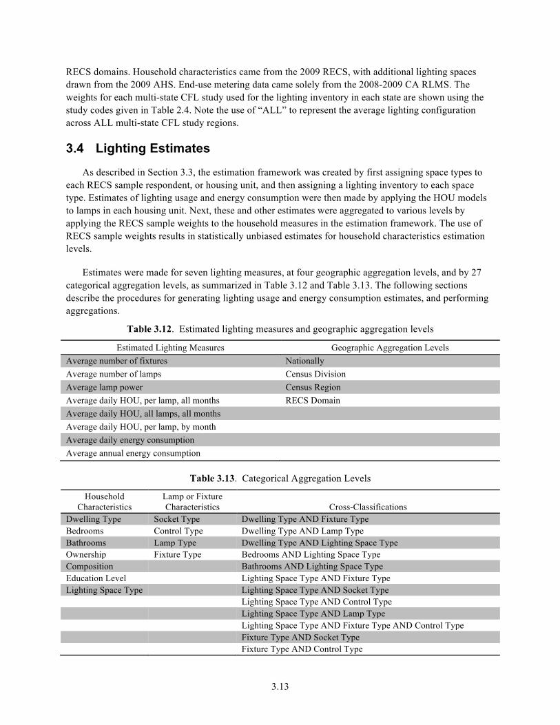
Estimates were made for seven lighting measures, at four geographic aggregation levels, and by 27 categorical aggregation levels, as summarized in Table 3.12 and Table 3.13. The following sections describe the procedures for generating lighting usage and energy consumption estimates, and performing aggregations.

Table 3.12. Estimated lighting measures and geographic aggregation levels

Estimated Lighting Measures Geographic Aggregation Levels Average number of fixtures Nationally Average number of lamps Census Division Average lamp power Census Region Average daily HOU, per lamp, all months RECS Domain Average daily HOU, all lamps, all months Average daily HOU, per lamp, by month Average daily energy consumption Average annual energy consumption

Table 3.13. Categorical Aggregation Levels

Household Characteristics

Lamp or Fixture Characteristics Cross-Classifications

Dwelling Type Bedrooms Bathrooms

Socket Type Control Type Lamp Type

Dwelling Type AND Fixture Type Dwelling Type AND Lamp Type Dwelling Type AND Lighting Space Type

Ownership Fixture Type Bedrooms AND Lighting Space Type Composition Bathrooms AND Lighting Space Type Education Level Lighting Space Type AND Fixture Type Lighting Space Type Lighting Space Type AND Socket Type

Lighting Space Type AND Control Type Lighting Space Type AND Lamp Type Lighting Space Type AND Fixture Type AND Control Type Fixture Type AND Socket Type Fixture Type AND Control Type

3.13

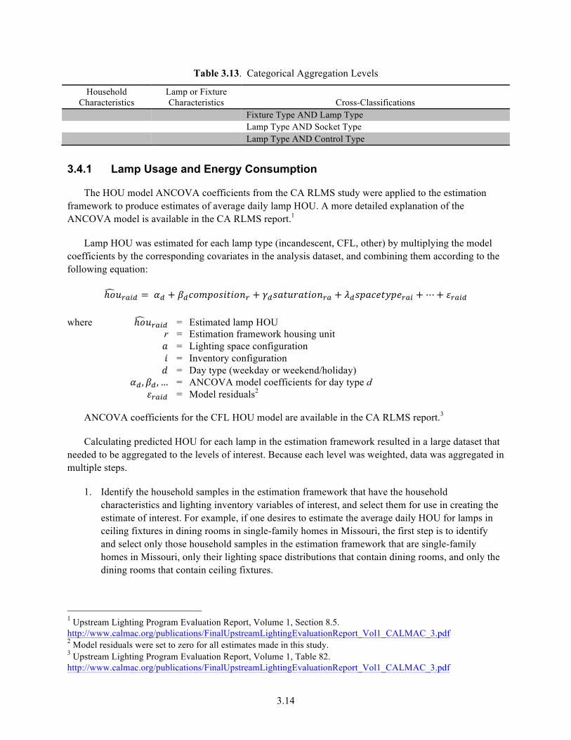
Table 3.13. Categorical Aggregation Levels

Household Lamp or Fixture Characteristics Characteristics Cross-Classifications

Fixture Type AND Lamp Type Lamp Type AND Socket Type Lamp Type AND Control Type

ℎ!!!"#$

3.4.1 Lamp Usage and Energy Consumption

The HOU model ANCOVA coefficients from the CA RLMS study were applied to the estimation framework to produce estimates of average daily lamp HOU. A more detailed explanation of the ANCOVA model is available in the CA RLMS report.1

Lamp HOU was estimated for each lamp type (incandescent, CFL, other) by multiplying the model coefficients by the corresponding covariates in the analysis dataset, and combining them according to the following equation:

= !!! + !!!"#$"%&'&"!! + !!!"#$%"#&'!!" + !!!"#$%&'"!!"# +⋯+ !!"#$

where ℎ!!!"#$ = Estimated lamp HOU r = Estimation framework housing unit ! = Lighting space configuration ! = Inventory configuration ! = Day type (weekday or weekend/holiday)

!! , !! , … = ANCOVA model coefficients for day type d!!"#$ = Model residuals2

ANCOVA coefficients for the CFL HOU model are available in the CA RLMS report.3

Calculating predicted HOU for each lamp in the estimation framework resulted in a large dataset that needed to be aggregated to the levels of interest. Because each level was weighted, data was aggregated in multiple steps.

1. Identify the household samples in the estimation framework that have the household characteristics and lighting inventory variables of interest, and select them for use in creating the estimate of interest. For example, if one desires to estimate the average daily HOU for lamps in ceiling fixtures in dining rooms in single-family homes in Missouri, the first step is to identify and select only those household samples in the estimation framework that are single-family homes in Missouri, only their lighting space distributions that contain dining rooms, and only the dining rooms that contain ceiling fixtures.

1 Upstream Lighting Program Evaluation Report, Volume 1, Section 8.5. http://www.calmac.org/publications/FinalUpstreamLightingEvaluationReport_Vol1_CALMAC_3.pdf2 Model residuals were set to zero for all estimates made in this study. 3 Upstream Lighting Program Evaluation Report, Volume 1, Table 82. http://www.calmac.org/publications/FinalUpstreamLightingEvaluationReport_Vol1_CALMAC_3.pdf

3.14

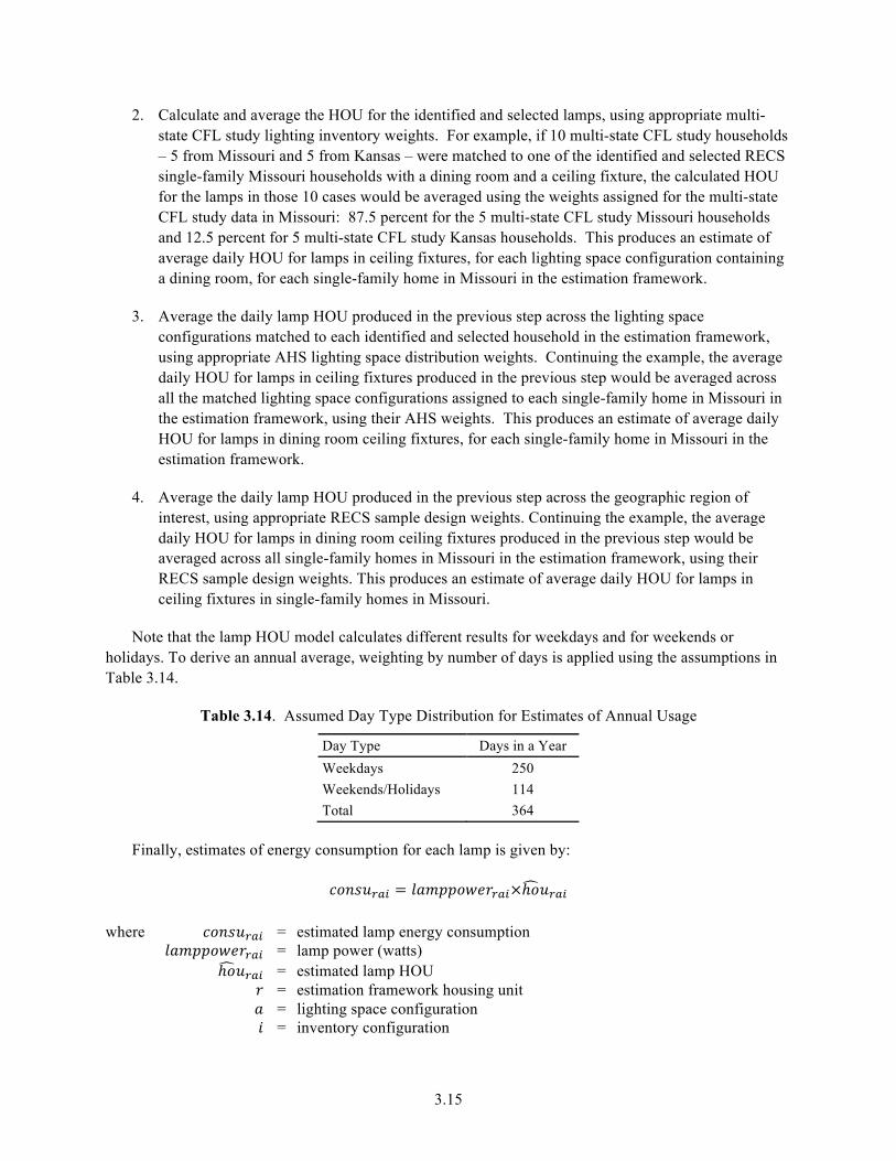
2. Calculate and average the HOU for the identified and selected lamps, using appropriate multi-state CFL study lighting inventory weights. For example, if 10 multi-state CFL study households – 5 from Missouri and 5 from Kansas – were matched to one of the identified and selected RECS single-family Missouri households with a dining room and a ceiling fixture, the calculated HOU for the lamps in those 10 cases would be averaged using the weights assigned for the multi-state CFL study data in Missouri: 87.5 percent for the 5 multi-state CFL study Missouri households and 12.5 percent for 5 multi-state CFL study Kansas households. This produces an estimate of average daily HOU for lamps in ceiling fixtures, for each lighting space configuration containing a dining room, for each single-family home in Missouri in the estimation framework.

3. Average the daily lamp HOU produced in the previous step across the lighting space configurations matched to each identified and selected household in the estimation framework, using appropriate AHS lighting space distribution weights. Continuing the example, the average daily HOU for lamps in ceiling fixtures produced in the previous step would be averaged across all the matched lighting space configurations assigned to each single-family home in Missouri in the estimation framework, using their AHS weights. This produces an estimate of average daily HOU for lamps in dining room ceiling fixtures, for each single-family home in Missouri in the estimation framework.

4. Average the daily lamp HOU produced in the previous step across the geographic region of interest, using appropriate RECS sample design weights. Continuing the example, the average daily HOU for lamps in dining room ceiling fixtures produced in the previous step would be averaged across all single-family homes in Missouri in the estimation framework, using their RECS sample design weights. This produces an estimate of average daily HOU for lamps in ceiling fixtures in single-family homes in Missouri.

Note that the lamp HOU model calculates different results for weekdays and for weekends or holidays. To derive an annual average, weighting by number of days is applied using the assumptions in Table 3.14.

Table 3.14. Assumed Day Type Distribution for Estimates of Annual Usage

Day Type Days in a Year Weekdays 250 Weekends/Holidays 114 Total 364

Finally, estimates of energy consumption for each lamp is given by:

!"#$!!"# = !"#$$%&'!!"#×ℎ!!!"#

where !"#$!!"# = estimated lamp energy consumption !"#$$%&'!!"# = lamp power (watts)

ℎ!!!"# = estimated lamp HOU ! = estimation framework housing unit ! = lighting space configuration ! = inventory configuration

3.15

Average lamp power and energy consumption estimates were aggregated from the composite dataset using the same procedure used for aggregating lighting usage.

3.4.2 Seasonal Variation

The ANCOVA models produced by the CA RLMS estimated the average lamp HOU per day over the course of a year. These models were created by annualizing each set of end-use metering data (which typically was only collected over a portion of the year) using a sinusoidal regression model. Re-applying the sinusoidal fit to the annualized estimate can create estimates of HOU within the year. This procedure was used to generate estimates of average daily HOU per lamp, by month. The annualization procedure is described in greater detail in the CA RLMS report.1

3.4.3 Number of Fixtures and Lamps

Estimates for the number of fixtures and lamps were generated by aggregating from the composite dataset to the levels of interest using the same procedure delineated in the previous section for creating lamp power, lamp usage, and energy consumption estimates.

1 Upstream Lighting Program Evaluation Report, Volume 1, Section 8.5. http://www.calmac.org/publications/FinalUpstreamLightingEvaluationReport_Vol1_CALMAC_3.pdf

3.16

4.0 Initial Estimation Highlights

This study distinguishes itself from previous residential lighting stock and energy consumption studies in that the estimates were generated using a bottom-up analysis and produced for both the entire United States and at various regional levels. The full set of estimates produced by this study, as described in Section 3.4, is provided in a companion spreadsheet. A select number of these estimates are presented here, focusing on comparisons of high-level estimates with previous studies, the ability to see regional variation courtesy of the RECS-based estimation framework, and the ability to produce cross-classifications afforded by the bottom-up analysis.

By definition, all statistical estimates have limitations. As described previously, the estimates produced by this study were not derived from new primary data or a single dataset. They are the result of a meta-analysis of datasets from previous residential lighting studies. While each of the datasets used was the best and most recent of its kind, the studies that produced them all had a more limited scope than this study set out to achieve. As a result, all estimates presented here should be viewed in the context of their accuracy and validity, which is discussed in detail in Section 5.0.

Finally, a consequence of using data sources from studies conducted over a span of years is that the estimates do not reflect one specific year. The data used in this study were collected between 2008 and 2010. The 2009 RECS household interviews began in early 2010 and were completed later that year.1 The 2009 AHS data was similarly collected in 2010, while the multi-state CFL study and CA RLMS were conducted over 2008-2009. Because all data sources collected data in 2010, the results are best presented as 2010 estimates, with the aforementioned caveats.

4.1 Total Energy Consumption

The residential sector consumed an estimated 194.1 TWh of electricity for lighting annually in and around 2010, as computed using the bottom-up aggregation described previously. A top-down estimate of total lighting energy consumed results in 206.6 TWh (i.e., 1.6 HOU per lamp × 47.7 watts per lamp × 67.4 lamps per home × 365 days per year × 113,566,400 homes in the United States). The bottom-up estimate is more accurate because it incorporates specific lamp-level attribute relationships from the source data that are lost in top-down energy consumption calculations.

This bottom-up estimate was greater than the recent 2010 Lighting Market Characterization (LMC) Study residential estimate of roughly 175 TWh. The LMC estimated a larger HOU (1.8 vs. 1.6) and a lower average number of lamps per home (51.4 vs. 67.4). The average lamp power between the two studies was very close, with 46 W estimated in the LMC and 47.7 W estimated in this study.

Table 4.1 gives an estimation of the average daily energy consumption (in kWh) for lighting for each of the 27 domains available in the 2009 RECS, along with estimates of the average number of lamps per housing unit, average daily HOU per lamp, and average lamp power. The 2009 RECS Mountain North domain, consisting of Idaho, Montana, Utah, and Wyoming, had the highest estimated average daily lighting energy consumption per household. This was driven primarily by the high percentage (86

1 Energy consumption was collected through the RECS Energy Supplier Survey for the 2009 calendar year, to be subsequently linked to the household characteristics data collected in 2010.

4.1

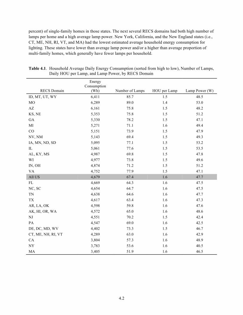
percent) of single-family homes in those states. The next several RECS domains had both high number of lamps per home and a high average lamp power. New York, California, and the New England states (i.e., CT, ME, NH, RI, VT, and MA) had the lowest estimated average household energy consumption for lighting. These states have lower than average lamp power and/or a higher than average proportion of multi-family homes, which generally have fewer lamps per household.

Table 4.1. Household Average Daily Energy Consumption (sorted from high to low), Number of Lamps, Daily HOU per Lamp, and Lamp Power, by RECS Domain

Energy Consumption

RECS Domain (Wh) Number of Lamps HOU per Lamp Lamp Power (W) ID, MT, UT, WY 6,411 85.7 1.5 48.5 MO 6,289 89.0 1.4 53.0 AZ 6,161 75.8 1.5 48.2 KS, NE 5,353 75.8 1.5 51.2 GA 5,330 78.2 1.5 47.1 MI 5,271 71.1 1.6 49.4 CO 5,151 73.9 1.5 47.9 NV, NM 5,143 69.4 1.5 49.3 IA, MN, ND, SD 5,095 77.1 1.5 53.2 IL 5,061 77.6 1.5 53.5 AL, KY, MS 4,987 69.8 1.5 47.8 WI 4,977 73.8 1.5 49.6 IN, OH 4,874 71.2 1.5 51.2 VA 4,752 77.9 1.5 47.1 All US 4,679 67.4 1.6 47.7 FL 4,669 64.3 1.6 47.5 NC, SC 4,654 64.7 1.6 47.5 TN 4,638 64.6 1.6 47.7 TX 4,617 63.4 1.6 47.3 AR, LA, OK 4,598 59.8 1.6 47.6 AK, HI, OR, WA 4,572 65.0 1.6 48.6 NJ 4,551 70.2 1.5 42.4 PA 4,547 69.0 1.6 42.5 DE, DC, MD, WV 4,402 73.3 1.5 46.7 CT, ME, NH, RI, VT 4,289 63.0 1.6 42.9 CA 3,804 57.3 1.6 48.9 NY 3,783 53.6 1.6 40.5 MA 3,405 51.9 1.6 46.5

4.2

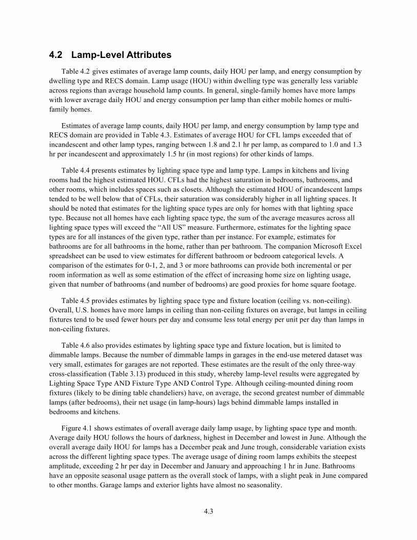
4.2 Lamp-Level Attributes Table 4.2 gives estimates of average lamp counts, daily HOU per lamp, and energy consumption by

dwelling type and RECS domain. Lamp usage (HOU) within dwelling type was generally less variable across regions than average household lamp counts. In general, single-family homes have more lamps with lower average daily HOU and energy consumption per lamp than either mobile homes or multi-family homes.

Estimates of average lamp counts, daily HOU per lamp, and energy consumption by lamp type and RECS domain are provided in Table 4.3. Estimates of average HOU for CFL lamps exceeded that of incandescent and other lamp types, ranging between 1.8 and 2.1 hr per lamp, as compared to 1.0 and 1.3 hr per incandescent and approximately 1.5 hr (in most regions) for other kinds of lamps.

Table 4.4 presents estimates by lighting space type and lamp type. Lamps in kitchens and living rooms had the highest estimated HOU. CFLs had the highest saturation in bedrooms, bathrooms, and other rooms, which includes spaces such as closets. Although the estimated HOU of incandescent lamps tended to be well below that of CFLs, their saturation was considerably higher in all lighting spaces. It should be noted that estimates for the lighting space types are only for homes with that lighting space type. Because not all homes have each lighting space type, the sum of the average measures across all lighting space types will exceed the “All US” measure. Furthermore, estimates for the lighting space types are for all instances of the given type, rather than per instance. For example, estimates for bathrooms are for all bathrooms in the home, rather than per bathroom. The companion Microsoft Excel spreadsheet can be used to view estimates for different bathroom or bedroom categorical levels. A comparison of the estimates for 0-1, 2, and 3 or more bathrooms can provide both incremental or per room information as well as some estimation of the effect of increasing home size on lighting usage, given that number of bathrooms (and number of bedrooms) are good proxies for home square footage.

Table 4.5 provides estimates by lighting space type and fixture location (ceiling vs. non-ceiling). Overall, U.S. homes have more lamps in ceiling than non-ceiling fixtures on average, but lamps in ceiling fixtures tend to be used fewer hours per day and consume less total energy per unit per day than lamps in non-ceiling fixtures.

Table 4.6 also provides estimates by lighting space type and fixture location, but is limited to dimmable lamps. Because the number of dimmable lamps in garages in the end-use metered dataset was very small, estimates for garages are not reported. These estimates are the result of the only three-way cross-classification (Table 3.13) produced in this study, whereby lamp-level results were aggregated by Lighting Space Type AND Fixture Type AND Control Type. Although ceiling-mounted dining room fixtures (likely to be dining table chandeliers) have, on average, the second greatest number of dimmable lamps (after bedrooms), their net usage (in lamp-hours) lags behind dimmable lamps installed in bedrooms and kitchens.

Figure 4.1 shows estimates of overall average daily lamp usage, by lighting space type and month. Average daily HOU follows the hours of darkness, highest in December and lowest in June. Although the overall average daily HOU for lamps has a December peak and June trough, considerable variation exists across the different lighting space types. The average usage of dining room lamps exhibits the steepest amplitude, exceeding 2 hr per day in December and January and approaching 1 hr in June. Bathrooms have an opposite seasonal usage pattern as the overall stock of lamps, with a slight peak in June compared to other months. Garage lamps and exterior lights have almost no seasonality.

4.3

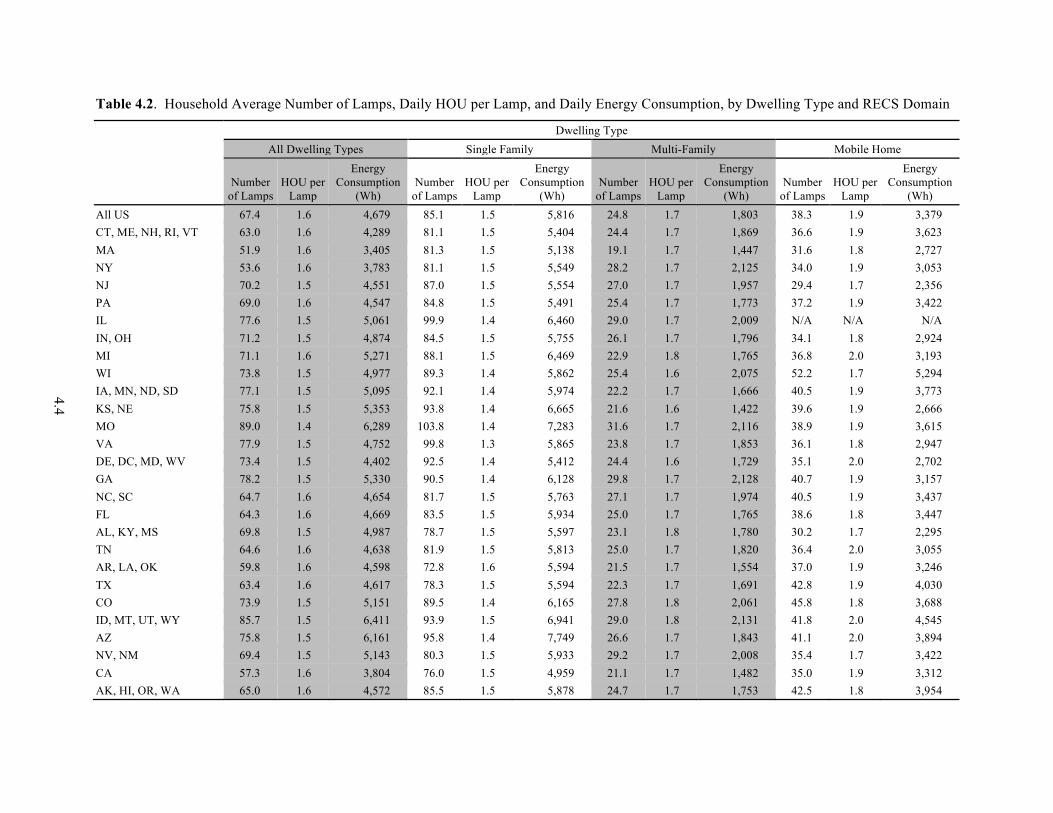
Table 4.2. Household Average Number of Lamps, Daily HOU per Lamp, and Daily Energy Consumption, by Dwelling Type and RECS Domain

Dwelling Type All Dwelling Types Single Family Multi-Family Mobile Home

4.4

Number of Lamps

HOU per Lamp

Energy Consumption

(Wh) Number

of Lamps HOU per

Lamp

Energy Consumption

(Wh) Number

of Lamps HOU per

Lamp

Energy Consumption

(Wh) Number

of Lamps HOU per

Lamp

Energy Consumption

(Wh) All US 67.4 1.6 4,679 85.1 1.5 5,816 24.8 1.7 1,803 38.3 1.9 3,379 CT, ME, NH, RI, VT 63.0 1.6 4,289 81.1 1.5 5,404 24.4 1.7 1,869 36.6 1.9 3,623 MA 51.9 1.6 3,405 81.3 1.5 5,138 19.1 1.7 1,447 31.6 1.8 2,727 NY 53.6 1.6 3,783 81.1 1.5 5,549 28.2 1.7 2,125 34.0 1.9 3,053 NJ 70.2 1.5 4,551 87.0 1.5 5,554 27.0 1.7 1,957 29.4 1.7 2,356 PA 69.0 1.6 4,547 84.8 1.5 5,491 25.4 1.7 1,773 37.2 1.9 3,422 IL 77.6 1.5 5,061 99.9 1.4 6,460 29.0 1.7 2,009 N/A N/A N/A IN, OH 71.2 1.5 4,874 84.5 1.5 5,755 26.1 1.7 1,796 34.1 1.8 2,924 MI 71.1 1.6 5,271 88.1 1.5 6,469 22.9 1.8 1,765 36.8 2.0 3,193 WI 73.8 1.5 4,977 89.3 1.4 5,862 25.4 1.6 2,075 52.2 1.7 5,294 IA, MN, ND, SD 77.1 1.5 5,095 92.1 1.4 5,974 22.2 1.7 1,666 40.5 1.9 3,773 KS, NE 75.8 1.5 5,353 93.8 1.4 6,665 21.6 1.6 1,422 39.6 1.9 2,666 MO 89.0 1.4 6,289 103.8 1.4 7,283 31.6 1.7 2,116 38.9 1.9 3,615 VA 77.9 1.5 4,752 99.8 1.3 5,865 23.8 1.7 1,853 36.1 1.8 2,947 DE, DC, MD, WV 73.4 1.5 4,402 92.5 1.4 5,412 24.4 1.6 1,729 35.1 2.0 2,702 GA 78.2 1.5 5,330 90.5 1.4 6,128 29.8 1.7 2,128 40.7 1.9 3,157 NC, SC 64.7 1.6 4,654 81.7 1.5 5,763 27.1 1.7 1,974 40.5 1.9 3,437 FL 64.3 1.6 4,669 83.5 1.5 5,934 25.0 1.7 1,765 38.6 1.8 3,447 AL, KY, MS 69.8 1.5 4,987 78.7 1.5 5,597 23.1 1.8 1,780 30.2 1.7 2,295 TN 64.6 1.6 4,638 81.9 1.5 5,813 25.0 1.7 1,820 36.4 2.0 3,055 AR, LA, OK 59.8 1.6 4,598 72.8 1.6 5,594 21.5 1.7 1,554 37.0 1.9 3,246 TX 63.4 1.6 4,617 78.3 1.5 5,594 22.3 1.7 1,691 42.8 1.9 4,030 CO 73.9 1.5 5,151 89.5 1.4 6,165 27.8 1.8 2,061 45.8 1.8 3,688 ID, MT, UT, WY 85.7 1.5 6,411 93.9 1.5 6,941 29.0 1.8 2,131 41.8 2.0 4,545 AZ 75.8 1.5 6,161 95.8 1.4 7,749 26.6 1.7 1,843 41.1 2.0 3,894 NV, NM 69.4 1.5 5,143 80.3 1.5 5,933 29.2 1.7 2,008 35.4 1.7 3,422 CA 57.3 1.6 3,804 76.0 1.5 4,959 21.1 1.7 1,482 35.0 1.9 3,312 AK, HI, OR, WA 65.0 1.6 4,572 85.5 1.5 5,878 24.7 1.7 1,753 42.5 1.8 3,954

4.5

Table 4.3. Household Average Number of Lamps, Daily HOU per Lamp, and Daily Energy Consumption, by Lamp Type and RECS Domain

Lamp Type All Lamp Types Incandescent CFL Other Lamp Type

Number of Lamps

HOU per Lamp

Energy Consumption

(Wh) Number

of Lamps HOU per

Lamp

Energy Consumption

(Wh) Number

of Lamps HOU per

Lamp

Energy Consumption

(Wh) Number

of Lamps HOU per

Lamp

Energy Consumption

(Wh) All US 67.4 1.6 4,679 41.9 1.2 2,932 14.3 1.9 411 11.2 1.5 1,341 CT, ME, NH, RI, VT 63.0 1.6 4,289 35.4 1.3 2,541 15.8 2.0 485 11.9 1.5 1,264 MA 51.9 1.6 3,405 28.5 1.3 2,067 14.0 2.1 423 9.5 1.5 916 NY 53.6 1.6 3,783 31.3 1.3 2,228 12.8 2.0 390 9.6 1.5 1,166 NJ 70.2 1.5 4,551 43.1 1.2 2,956 15.7 1.9 434 11.4 1.5 1,160 PA 69.0 1.6 4,547 41.6 1.2 2,808 15.4 2.0 435 12.1 1.5 1,304 IL 77.6 1.5 5,061 50.3 1.2 3,451 16.6 1.9 463 10.7 1.3 1,148 IN, OH 71.2 1.5 4,874 48.4 1.2 3,356 11.8 2.0 361 10.9 1.4 1,158 MI 71.1 1.6 5,271 46.6 1.3 3,350 11.9 2.0 339 12.5 1.5 1,582 WI 73.8 1.5 4,977 48.6 1.2 3,761 15.9 1.9 516 9.4 1.4 740 IA, MN, ND, SD 77.1 1.5 5,095 46.8 1.2 3,366 17.4 1.9 486 12.8 1.4 1,243 KS, NE 75.8 1.5 5,353 46.6 1.2 3,171 17.0 1.9 447 12.2 1.4 1,791 MO 89.0 1.4 6,289 53.4 1.2 3,469 18.2 1.8 483 17.5 1.3 2,338 VA 77.9 1.5 4,752 50.7 1.2 3,332 15.9 1.8 375 11.2 1.4 1,046 DE, DC, MD, WV 73.4 1.5 4,402 50.3 1.2 3,295 13.6 1.8 336 9.5 1.4 771 GA 78.2 1.5 5,330 49.5 1.2 3,396 16.1 1.8 438 12.6 1.5 1,515 NC, SC 64.7 1.6 4,654 41.0 1.2 2,907 13.5 1.9 384 10.2 1.6 1,373 FL 64.3 1.6 4,669 40.8 1.2 2,863 13.3 1.9 384 10.3 1.6 1,429 AL, KY, MS 69.8 1.5 4,987 44.1 1.2 3,110 14.2 1.9 407 11.5 1.5 1,471 TN 64.6 1.6 4,638 40.6 1.3 2,881 13.5 2.0 398 10.5 1.5 1,359 AR, LA, OK 59.8 1.6 4,598 38.3 1.3 2,901 12.3 2.0 371 9.2 1.6 1,327 TX 63.4 1.6 4,617 41.4 1.3 3,022 12.9 2.0 370 9.1 1.6 1,230 CO 73.9 1.5 5,151 45.2 1.2 3,054 15.3 1.8 412 13.4 1.4 1,690 ID, MT, UT, WY 85.7 1.5 6,411 52.4 1.2 3,747 17.6 1.9 520 15.7 1.5 2,145 AZ 75.8 1.5 6,161 41.2 1.2 2,837 17.4 1.8 496 17.2 1.6 2,851 NV, NM 69.4 1.5 5,143 41.2 1.2 2,865 15.1 1.8 437 13.1 1.6 1,841 CA 57.3 1.6 3,804 32.3 1.2 2,183 13.8 1.9 417 11.2 1.6 1,204 AK, HI, OR, WA 65.0 1.6 4,572 40.2 1.2 2,816 13.5 1.9 396 11.4 1.5 1,362

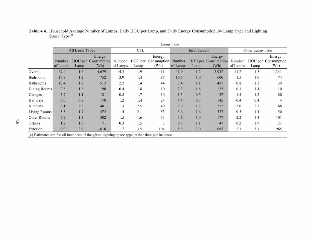
4.6

Table 4.4. Household Average Number of Lamps, Daily HOU per Lamp, and Daily Energy Consumption, by Lamp Type and Lighting Space Type(a)

Lamp Type All Lamp Types CFL Incandescent Other Lamp Type

Number of Lamps

HOU per Lamp

Energy Consumption

(Wh) Number

of Lamps HOU per

Lamp

Energy Consumption

(Wh) Number

of Lamps HOU per

Lamp

Energy Consumption

(Wh) Number

of Lamps HOU per

Lamp

Energy Consumption

(Wh) Overall 67.4 1.6 4,679 14.3 1.9 411 41.9 1.2 2,932 11.2 1.5 1,341 Bedrooms 15.9 1.2 752 3.9 1.4 87 10.5 1.0 600 1.5 1.0 74 Bathrooms 10.4 1.2 512 2.2 1.4 44 7.4 1.1 435 0.8 1.2 39 Dining Rooms 2.8 1.6 190 0.4 1.8 10 2.3 1.6 175 0.1 1.4 10 Garages 3.2 1.1 121 0.5 1.7 16 1.3 0.5 37 1.4 1.2 80 Hallways 6.0 0.8 170 1.2 1.4 24 4.4 0.7 145 0.4 0.4 4 Kitchens 6.1 2.3 481 1.3 2.5 49 2.9 1.7 272 2.0 2.7 168 Living Rooms 5.5 1.7 472 1.4 2.1 53 3.6 1.6 377 0.5 1.4 50 Other Rooms 7.2 1.3 302 1.5 1.6 33 3.6 1.0 177 2.2 1.4 101 Offices 1.2 1.5 71 0.3 1.5 7 0.7 1.1 47 0.2 1.9 21 Exterior 9.0 2.9 1,610 1.7 3.5 104 5.3 2.0 695 2.1 3.1 965 (a) Estimates are for all instances of the given lighting space type, rather than per instance.

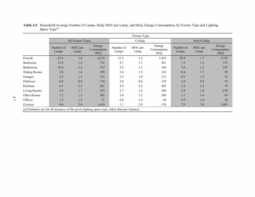
4.7

Table 4.5. Household Average Number of Lamps, Daily HOU per Lamp, and Daily Energy Consumption, by Fixture Type and Lighting Space Type(a)

Fixture Type All Fixture Types Ceiling Non-Ceiling

Number of Lamps

HOU per Lamp

Energy Consumption

(Wh)

Number of Lamps

HOU per Lamp

Energy Consumption

(Wh)

Number of Lamps

HOU per Lamp

Energy Consumption

(Wh) Overall 67.4 1.6 4,679 37.5 1.5 1,935 29.9 1.7 2,745 Bedrooms 15.9 1.2 752 8.7 1.1 381 7.2 1.3 375 Bathrooms 10.4 1.2 512 3.5 1.1 169 7.0 1.3 347 Dining Rooms 2.8 1.6 190 2.4 1.5 163 0.4 1.7 29 Garages 3.2 1.1 121 2.9 1.0 112 0.3 1.2 14 Hallways 6.0 0.8 170 5.0 0.8 138 1.0 0.9 35 Kitchens 6.1 2.3 481 4.9 2.2 405 1.2 2.4 79 Living Rooms 5.5 1.7 472 2.7 1.6 206 2.8 1.8 270 Other Rooms 7.2 1.3 302 5.6 1.2 209 1.7 1.4 95 Offices 1.2 1.5 71 0.8 1.4 44 0.5 1.6 29 Exterior 9.0 2.9 1,610 1.1 2.8 139 7.9 3.0 1,493 (a) Estimates are for all instances of the given lighting space type, rather than per instance.

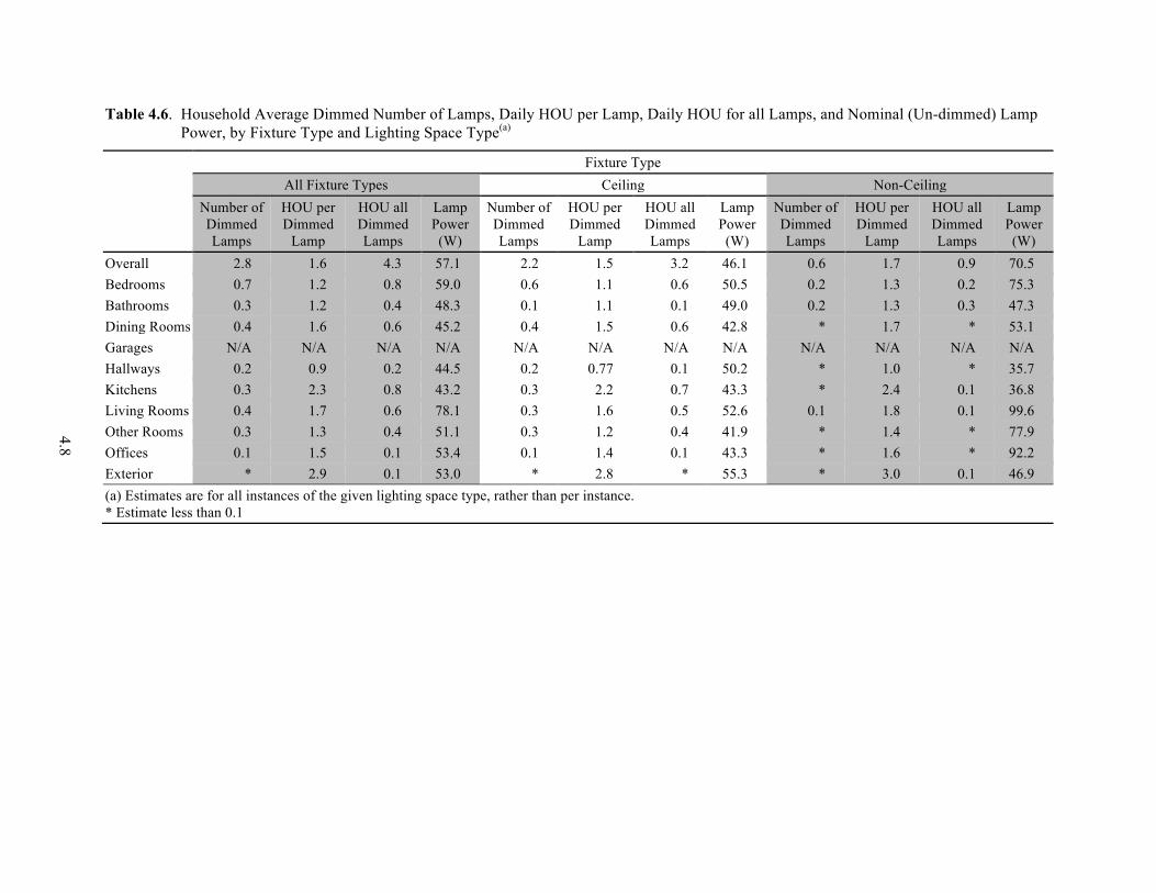
4.8

Table 4.6. Household Average Dimmed Number of Lamps, Daily HOU per Lamp, Daily HOU for all Lamps, and Nominal (Un-dimmed) Lamp Power, by Fixture Type and Lighting Space Type(a)

Fixture Type All Fixture Types Ceiling Non-Ceiling

Number of Dimmed Lamps

HOU per Dimmed

Lamp

HOU all Dimmed Lamps

Lamp Power (W)

Number of Dimmed Lamps

HOU per Dimmed

Lamp

HOU all Dimmed Lamps

Lamp Power (W)

Number of Dimmed Lamps

HOU per Dimmed

Lamp

HOU all Dimmed Lamps

Lamp Power (W)

Overall 2.8 1.6 4.3 57.1 2.2 1.5 3.2 46.1 0.6 1.7 0.9 70.5 Bedrooms 0.7 1.2 0.8 59.0 0.6 1.1 0.6 50.5 0.2 1.3 0.2 75.3 Bathrooms 0.3 1.2 0.4 48.3 0.1 1.1 0.1 49.0 0.2 1.3 0.3 47.3 Dining Rooms 0.4 1.6 0.6 45.2 0.4 1.5 0.6 42.8 * 1.7 * 53.1 Garages N/A N/A N/A N/A N/A N/A N/A N/A N/A N/A N/A N/A Hallways 0.2 0.9 0.2 44.5 0.2 0.77 0.1 50.2 * 1.0 * 35.7 Kitchens 0.3 2.3 0.8 43.2 0.3 2.2 0.7 43.3 * 2.4 0.1 36.8 Living Rooms 0.4 1.7 0.6 78.1 0.3 1.6 0.5 52.6 0.1 1.8 0.1 99.6 Other Rooms 0.3 1.3 0.4 51.1 0.3 1.2 0.4 41.9 * 1.4 * 77.9 Offices 0.1 1.5 0.1 53.4 0.1 1.4 0.1 43.3 * 1.6 * 92.2 Exterior * 2.9 0.1 53.0 * 2.8 * 55.3 * 3.0 0.1 46.9 (a) Estimates are for all instances of the given lighting space type, rather than per instance. * Estimate less than 0.1

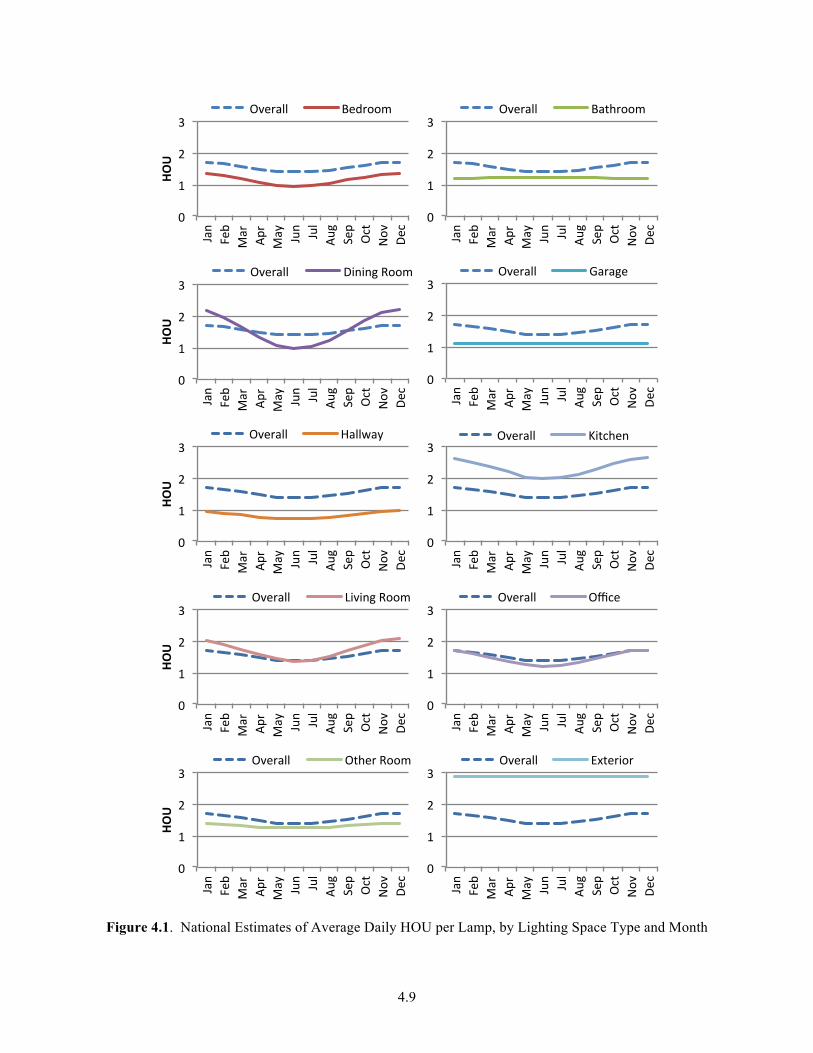
4.9

Figure 4.1. National Estimates of Average Daily HOU per Lamp, by Lighting Space Type and Month

0"

1"

2"

3"

Jan"

Feb"

Mar"

Apr"

May"

Jun" Jul"

Aug"

Sep"

Oct"

Nov"

Dec"

HOU$

Overall" Exterior"

0"

1"

2"

3"

Jan"

Feb"

Mar"

Apr"

May"

Jun" Jul"

Aug"

Sep"

Oct"

Nov"

Dec"

HOU$

Overall" Other"Room"

0"

1"

2"

3"

Jan"

Feb"

Mar"

Apr"

May"

Jun" Jul"

Aug"

Sep"

Oct"

Nov"

Dec"

HOU$

Overall" Office"

0"

1"

2"

3"

Jan"

Feb"

Mar"

Apr"

May"

Jun" Jul"

Aug"

Sep"

Oct"

Nov"

Dec"

HOU$

Overall" Living"Room"

0"

1"

2"

3"Jan"

Feb"

Mar"

Apr"

May"

Jun" Jul"

Aug"

Sep"

Oct"

Nov"

Dec"

HOU$

Overall" Kitchen"

0"

1"

2"

3"

Jan"

Feb"

Mar"

Apr"

May"

Jun" Jul"

Aug"

Sep"

Oct"

Nov"

Dec"

HOU$

Overall" Hallway"

0"

1"

2"

3"

Jan"

Feb"

Mar"

Apr"

May"

Jun" Jul"

Aug"

Sep"

Oct"

Nov"

Dec"

HOU$

Overall" Garage"

0"

1"

2"

3"

Jan"

Feb"

Mar"

Apr"

May"

Jun" Jul"

Aug"

Sep"

Oct"

Nov"

Dec"

HOU$

Overall" Dining"Room"

0"

1"

2"

3"

Jan"

Feb"

Mar"

Apr"

May"

Jun" Jul"

Aug"

Sep"

Oct"

Nov"

Dec"

HOU$

Overall" Bathroom"

0"

1"

2"

3"

Jan"

Feb"

Mar"

Apr"

May"

Jun" Jul"

Aug"

Sep"

Oct"

Nov"

Dec"

HOU$

Overall" Bedroom"

5.1

5.0 Accuracy and Validity of the Estimates

As discussed in previous sections, the estimates presented in this report and in the companion spreadsheet are the result of an analysis linking estimates from four related studies. Each of these studies was designed to be unbiased and achieve a certain degree of accuracy within its original domain. This study uses various methods to extend data from these studies to other domains. The scope of each study was limited to specific geographic regions or in the collected lighting information:

• The CA RLMS ANCOVA model relates lighting HOU to within-household unit and demographic characteristics, for California households only. The model has not yet been calibrated to account for this relationship in other regions of the country.

• The 2009 RECS did not collect room-level inventory of fixture characteristics or usage data from direct metering.

• The 2009 AHS did not collect fixture characteristics and usage data within rooms of homes, and geographic identifiers at finer levels than the four census regions were not made public.

• The Multi-State CFL Modeling Study consisted of several regional studies, corresponding with states or electric utility service territories. The collection of these regional studies had very good coverage in some areas of the United States and very little coverage in others. Although the studies had both overall household and room-level luminaire characteristics, direct metering of lamps was not part of the study protocols.

The accuracy and validity of the estimates presented in this report and the companion spreadsheet are largely dependent on how representative the data collected in those restricted studies is for extension to the housing stock in other geographic areas, and the validity of the assumptions underlying the methods used to make those extensions. The bias in the estimates created by the data linking processes used is unknown. There are, however, controls in place that flag estimates derived from fewer than ten RECS households or having a coefficient of variation associated with an HOU estimate greater than 50 percent. These data quality flags have been used in the 2009 and previous RECS. The CA RLMS generated HOU estimates with an overall 16 percent margin-of-error at 90 percent confidence1, which would serve as a best case when applying this model to linked data from other studies. Estimates generated here would necessarily be less accurate if regional inventory data used in the study were not reflective of the population or if lighting usage behavior varied significantly in different parts of the United States.

5.1 Comparison with CA RLMS Estimates

A simple method for validating the methodology used in this study is to compare the estimates for California produced by this study with those from the CA RLMS study. Although the CA RLMS relied solely on its sample of households to estimate HOU, this study leveraged information from various sources, including the RECS, the AHS, the multi-state CFL studies, and the CA RLMS itself. Nevertheless, the estimates for California from both studies are very similar. Table 5.1, Table 5.2, and Table 5.3 show the estimates of HOU from this study along with the CFL estimates from the CA RLMS.2 1 Upstream Lighting Program Evaluation Report, Volume 1, Table 84. http://www.calmac.org/publications/FinalUpstreamLightingEvaluationReport_Vol1_CALMAC_3.pdf 2 Upstream Lighting Program Evaluation Report, Volume 1, Table 85. http://www.calmac.org/publications/FinalUpstreamLightingEvaluationReport_Vol1_CALMAC_3.pdf

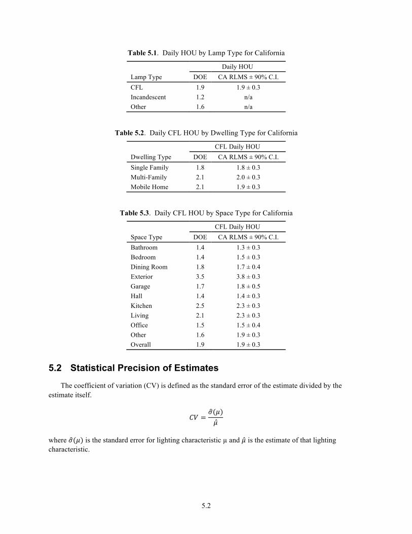
5.2

Table 5.1. Daily HOU by Lamp Type for California

Lamp Type

Daily HOU DOE CA RLMS ± 90% C.I.

CFL 1.9 1.9 ± 0.3 Incandescent 1.2 n/a Other 1.6 n/a

Table 5.2. Daily CFL HOU by Dwelling Type for California

Dwelling Type

CFL Daily HOU DOE CA RLMS ± 90% C.I.

Single Family 1.8 1.8 ± 0.3 Multi-Family 2.1 2.0 ± 0.3 Mobile Home 2.1 1.9 ± 0.3

Table 5.3. Daily CFL HOU by Space Type for California

Space Type

CFL Daily HOU DOE CA RLMS ± 90% C.I.

Bathroom 1.4 1.3 ± 0.3 Bedroom 1.4 1.5 ± 0.3 Dining Room 1.8 1.7 ± 0.4 Exterior 3.5 3.8 ± 0.3 Garage 1.7 1.8 ± 0.5 Hall 1.4 1.4 ± 0.3 Kitchen 2.5 2.3 ± 0.3 Living 2.1 2.3 ± 0.3 Office 1.5 1.5 ± 0.4 Other 1.6 1.9 ± 0.3 Overall 1.9 1.9 ± 0.3

5.2 Statistical Precision of Estimates

The coefficient of variation (CV) is defined as the standard error of the estimate divided by the estimate itself.

!" = !(!)!

where !(!) is the standard error for lighting characteristic µ and ! is the estimate of that lighting characteristic.

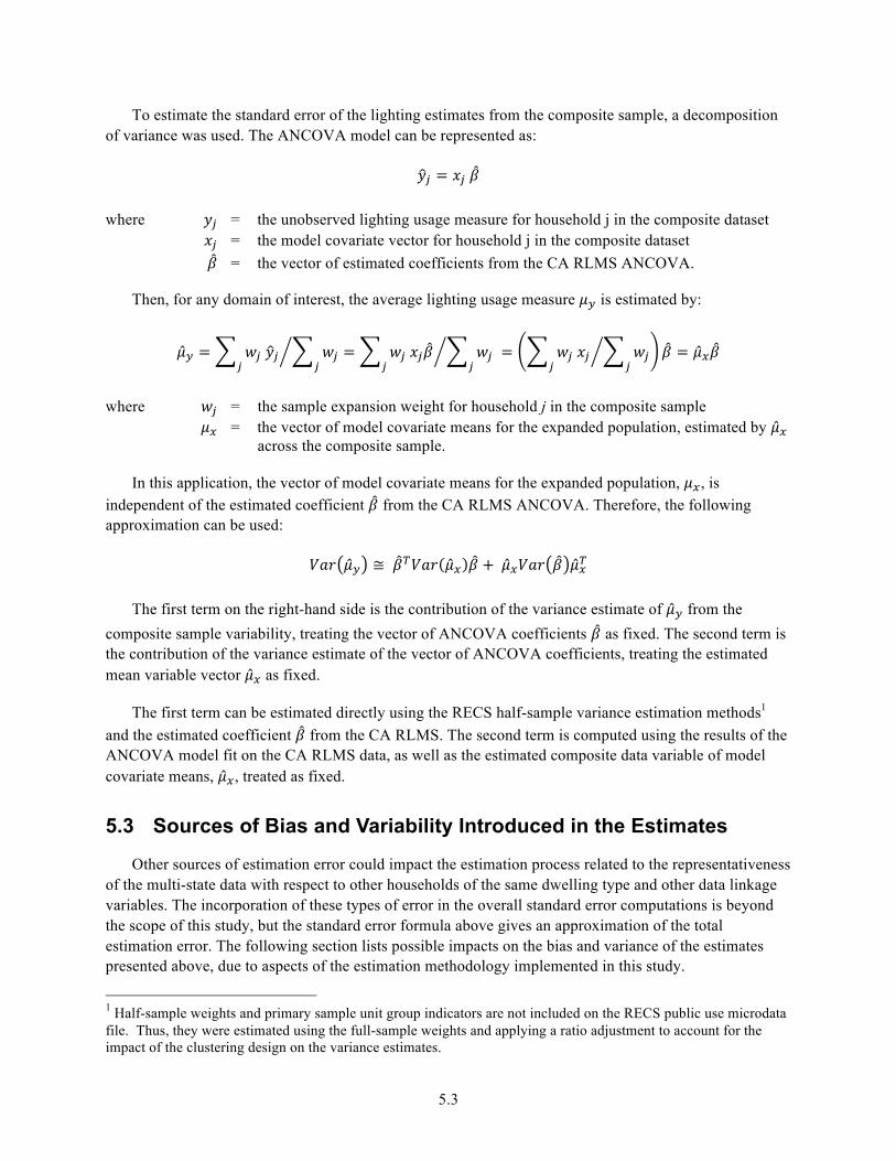
5.3

To estimate the standard error of the lighting estimates from the composite sample, a decomposition of variance was used. The ANCOVA model can be represented as:

!! = !! !!

where !! = the unobserved lighting usage measure for household j in the composite dataset !! = the model covariate vector for household j in the composite dataset ! = the vector of estimated coefficients from the CA RLMS ANCOVA.

Then, for any domain of interest, the average lighting usage measure !! is estimated by:

!! = !! !!!!

!!!

= !! !!!!!

!!!

!= !! !!!!

!!!

! = !!!

where !! = the sample expansion weight for household j in the composite sample !! = the vector of model covariate means for the expanded population, estimated by !!

across the composite sample.

In this application, the vector of model covariate means for the expanded population, !!, is independent of the estimated coefficient ! from the CA RLMS ANCOVA. Therefore, the following approximation can be used:

!"# !! ≅ !!!!"# !! ! + !!!!"# ! !!!

The first term on the right-hand side is the contribution of the variance estimate of !! from the composite sample variability, treating the vector of ANCOVA coefficients ! as fixed. The second term is the contribution of the variance estimate of the vector of ANCOVA coefficients, treating the estimated mean variable vector !! as fixed.

The first term can be estimated directly using the RECS half-sample variance estimation methods1 and the estimated coefficient ! from the CA RLMS. The second term is computed using the results of the ANCOVA model fit on the CA RLMS data, as well as the estimated composite data variable of model covariate means, !!, treated as fixed.

5.3 Sources of Bias and Variability Introduced in the Estimates

Other sources of estimation error could impact the estimation process related to the representativeness of the multi-state data with respect to other households of the same dwelling type and other data linkage variables. The incorporation of these types of error in the overall standard error computations is beyond the scope of this study, but the standard error formula above gives an approximation of the total estimation error. The following section lists possible impacts on the bias and variance of the estimates presented above, due to aspects of the estimation methodology implemented in this study.

1 Half-sample weights and primary sample unit group indicators are not included on the RECS public use microdata file. Thus, they were estimated using the full-sample weights and applying a ratio adjustment to account for the impact of the clustering design on the variance estimates.

5.4

1. Applying CA RLMS ANCOVA to other areas

a. Bias: Regional differences in patterns of equipment ownership and use result in biased estimates. The relationship between lighting usage and household and lighting source characteristics in California may be very different than in other regions of the country.

b. Variance: mainly captured in the RECS-type variance estimate, as discussed.

2. Imputing lighting inventory using the inventory samples and the AHS room-type distributions

a. Bias: For comprehensive inventory samples, bias is mainly due to geographic differences between the originally represented area and the areas the data are applied to.

b. Variability: For some multi-state study areas, the level of variability for certain subgroups of the population, such as mobile homes or very large homes, may be lower in the samples of inventory data than in the population.

3. Imputing room and lighting space type using AHS assignments

a. Bias: Probably minimal for aggregates at the census region level. If room-type distributions are very different within a region, in particular if the mix of high- and low-use rooms is very different, estimates for these finer areas will be systematically misstated.

b. Variability: The variability from AHS microdata is mainly the sampling variability of AHS itself. As noted, some of this is captured in the observed variability.

5.4 Opportunities for Improving Estimates

The estimates generated by this study could be readily improved by the availability of new regional data meeting defined pre-conditions and funding for its analysis. New end-use metering data would improve the accuracy for not only the geographic region the data came from and all RECS domains inclusive of that region, but likely also for nearby domains and possibly nationally.

For example, if New York conducted a statewide residential lighting inventory study that collected measures required by the HOU model, the estimation framework would be updated by replacing the inventory data previously used to represent New York, assuming this new data was determined to be an improvement of that which was previously used. This would, at minimum, improve the study estimates for New York, the Mid-Atlantic census division, the Northeast census region, and the United States. To the extent it could be determined that the new data was representative of other states or RECS-reportable domains listed in Table 3.11, the data could improve the estimates in other states. If a state was in a RECS-reportable domain that also included one or more other states, such as Connecticut, that conducted a statewide inventory study with relevant demographics to the HOU model, it could be possible to “break away” Connecticut from the other states in the RECS-reportable domain. This would depend on the sample design and other factors.

Continuing the example scenario, another level of improvement could be achieved if New York decided to instead conduct a statewide residential lighting metering study, collecting household characteristics, lighting inventory, and end-use metering data for each household following the protocols used in the CA RLMS. In addition to updating the estimation framework as described above, the HOU model could be calibrated for representative regions using the new metering data. This would eliminate potential bias in the existing New York estimates due to behavioral differences in how New Yorkers use

5.5

lighting in their homes as compared with Californians. Additional analysis would be conducted to determine the most appropriate way to use the New York and California metering data to improve the accuracy for applications of the HOU models in states other than New York and California.

Two datasets, available now or in the near future, have been identified that meet the requirements for incorporation into the estimation framework:

1. Household characteristics, lighting inventories, and end-use metering data were collected over 6 months in late 2012 from 183 households in the Mid-Atlantic census division, in an effort managed and executed by the authors of this study.

2. Household characteristics and lighting inventories were collected from over 1,850 households together with end-use metering data from a 101 household subset in the Pacific census division as part of the Northwest Energy Efficiency Alliance Residential Building Stock Assessment.1

The availability of additional funding for analyzing these datasets would lead to improved accuracy in multiple RECS domains.

1 http://neea.org/resource-center/regional-data-resources/residential-building-stock-assessment