research techniques in biomechanics
TRANSCRIPT

Research Techniques in Biomechanics
KIN 743
John A. Mercer, Ph.D.

KIN 743 ii
Writing Methods ........................................................................................................................... 1
Kinesiology..................................................................................................................................... 2
Introduction ................................................................................................................................... 4
Variables and Units....................................................................................................................... 5
Recording data .............................................................................................................................. 6
How to make an electrogoniometer ............................................................................................. 7
Sampling Rate ............................................................................................................................... 9
Electric Circuit Basics ................................................................................................................ 10
The Camera ................................................................................................................................. 11
Motion Analysis ........................................................................................................................... 14
Video analysis of motion ............................................................................................................. 15
Smoothing Data ........................................................................................................................... 16
3D Calibration ............................................................................................................................. 18
Joint Moments ............................................................................................................................. 19
Accelerometers ............................................................................................................................ 26
Impact Testing and Springs ....................................................................................................... 28
Electromyography....................................................................................................................... 30
Processing EMG .......................................................................................................................... 31
Isokinetic Dynamometer ............................................................................................................ 34
Energy .......................................................................................................................................... 35

KIN 743 1
Writing Methods
Journals may specify a format that the method section should follow. In many cases, the same
information is simply presented in different organizations. The common elements of many
journals are highlighted below. All reports should use this format unless a different format has
been specified.
Participants
Describe population of participants that were tested
Weight, height, age, gender
Experience in task, injuries (or lack of), …
Instrumentation
Describe the instruments used in the experiment
Model, manufacturer
Force platform (Kistler model 8600B, 60 x 30 cm)
Treadmill (Precor model 9.3)
A/D board type
Sample rate and period
Procedures Describe the experiment conducted – What were subjects asked to do?
Warm-up, conditions, order, instructions, etc.
Describe when data were collected
Data reduction
Describe how data were processed to yield the dependent variable(s)
Calculations that were made
Criteria to identify discrete parameters.
“Impact peak magnitude was recorded as the highest force within
50 ms of heel contact that was followed by a local force
minimum.”
You may want to include an example raw data set and illustrate
the processing steps to yield the dependent variable(s).
Statistical analysis
Specify statistical design
Dependent variables – for your semester project, select one or two
dependent variables.
Independent variables – for your semester project, it is strongly
suggested to design the experiment so a paired t-test can be used.*
Statistical procedures used
Repeated measures ANOVA, follow-up tests…
*For your semester project, you are not collecting data that will yield a
publication or presentation. The goal is to create a ‘practice’ data set that
demonstrates your knowledge of instrumentation.

KIN 743 2
Kinesiology
Kinesiology is ultimately the study of performance. For example, an exercise physiologist is interested in measuring
aerobic performance as well as training an individual to perform better. A person involved in Motor Control is
interested in how performance is controlled through the neuromuscular skeletal system. Someone interested in
Motor Learning is interested in how a person learns to control movements to increase performance.
Central Nervous System
Environment
Sport
Psychology
Motor Control
Muscles
(Internal Forces)
Force-Velocity
Length-Tension
VO2
Exercise
Physiology
Forces
Internal and External
Kinetics
Gravity (& other external forces)
Newton’s Laws of Motion
Law of Inertia
Law of Acceleration
Law of Action-Reaction
Motor
Learning
Biomechanics
Displacement & Time
Kinematics
Position
Velocity
Acceleration
Anatomical Movements
Anatomical
Kinesiology
Performance
In order to understand the factors affecting performance, it is essential that you, the student of Kinesiology, integrate
the information from all the courses offered in the Department of Kinesiology.

KIN 743 3
Terminology
Biomechanics
Kinematics
Types of motion
Displacement
Distance
Velocity
Speed
Acceleration
Representation of angles
Absolute vs. Relative angles
Angular displacement
Angular velocity
Angular speed
Angular acceleration
Relationship between linear and angular velocity and acceleration
Kinetics
Linear Kinetics
Newton’s Laws of Motion
Force
Mass
Inertia
Momentum
Impulse
Gravity
Ground reaction force
Projectile motion (vertical and horizontal)
Angular Kinetics
Torque
Moment
Axis of rotation
Line of application of a force
Center of mass/gravity
Moment of inertia
Moment arm
Mathematical skills
Slope
Trigonometric relationships (e.g., calculation of angels)
Composition and resolution of vectors
PVA models
Computing skills
Excel (or some spreadsheet software)
Graphing
Formulas
Functions
Matlab

KIN 743 4
Introduction
Topic Parameter Instrument
Anthropometrics Joint center
Segment masses
Segment COM
Segment moment of inertia
Table of norms
regression equations
models
direct measurement
Kinematics Time
Displacement
Velocity
Acceleration
Angular parameters
Momentum
Timers
Video recorder/TV
Cinematography
Accelerometers
Electrogoniometers
Computer simulation
Kinetics Forces
Impulse
Pressure
Pressure transducers
Force transducers
ma
modeling
Neuromuscular Muscle onsets
Contractile properties
Muscle sequencing
EMG
Indwelling EMG
Surface EMG
in vitro muscle testing
Common tools used in Biomechanics Research
Kinematics
Electrogoniometer
Auto digitizing
Cameras (e.g., Panasonic VHS cameras)
Accelerometer
Kinetics
Kistler force platform
Isokinetic dynamometer
Impact tester
Electromyography
Surface EMG
Synchronization
Elgon
Magnetic switch
Synch-box
Concepts commonly used in Biomechanics research
Sampling theorem
Mass-spring model
Joint moments
Smoothing

KIN 743 5
Variables and Units
Kinematic Parameter Symbol Unit
Time t s
Position
Cartesian
Horizontal x m
Vertical y m
Medial-lateral z m
Polar
Radius r m
Angle radians
Linear
displacement s m
velocity v m·s-1
acceleration a m·s-2
Angular
displacement Rad
velocity rad·s-1
acceleration rad·s-2
Linear Momentum H kgm/s
Angular Momentum h kgm2/s
Kinetic Parameter Symbol Unit
Force N Newton (kg·m·s-2)
Linear Impulse J Ns
Angular Impulse Nms
Torque Nm
Pressure Pa Pascal (N/m2)
Power W Watt (J/s)
Work U Joule
Energy E Joule
Other Symbol Unit
Mass m kg
Length l m
Time t s
Moment of inertia I kg·m2
Density kg/m3

KIN 743 6
Recording data
Analog vs. Digital signals
Analog: continuous time function.
Digital: discrete time function.
A/D converter
Transforms analog signals to digital format.
Analog signal can be represented by a voltage (e.g., elgon).
The voltage is converted to a digital form using an A/D converter.
Range: A/D converters have a range of voltages that it can detect, usually 10V or 5V.
Computers understand 0s and 1s, called a binary digit or bit.
Bits are converted to decimal form in the following manner:
111 = 22+21+20 = 4+2+1 = 7
110 = 22+21+0 = 4+2+0 = 6
101 = 22+0+20 = 4+0+1 = 5
100 = 22+0+0 = 4+0+0 = 4
011 = 0+21+20 = 0+2+1 = 3
010 = 0+21+0 = 0+2+0 = 2
001 = 0+0+20 = 0+0+1 = 1
000 = 0+0+0 = 0+0+0 = 0
The voltages are converted to binary digits and stored in the computer (e.g., RAM).
Resolution is defined as the number of bits that the A/D converter uses to represent the analog signal.
The higher the resolution, the greater the number of divisions of the voltage range can be made. This
results in more discrete voltage values that can be used to represent the analog signal. The resolution
of an A/D board is identified by the bit code. A 3-bit code has 8 codes (23) that can be used to
represent a signal. An 8-bit A/D board has 28 or 256 codes; a 16-bit A/D converter has 65536 codes.
For example, consider a 10V range of detectable voltages (i.e., 5V). If you have a 3 bit A/D
converter, the voltages that can be represented are:
Voltage Binary code
0 000
1.43 001
2.86 010
4.29 011
5.71 100
7.14 101
8.57 110
10.00 111
Therefore, a value of 4.9 V could not be represented accurately using a 3-Bit A/D converter (4.9 V
would be rounded to either 5.71 or 4.29 V depending on the A/D converter).
To calculate the voltage increment of the A/D converter, use the following formula:
Voltage increment = (range/(2bits-1)
Units
A/D units are in voltages, which must be converted back to correct units (e.g., degrees, N, g)
Relationship between voltage change and unit change must be linear.
Conversion formula
Units = (A/D voltage) * units/volt
For example, an accelerometer may have a conversion factor of 10 g/V. Therefore, if 2.5 V are
measured by the A/D board, an acceleration of 25g was recorded.

KIN 743 7
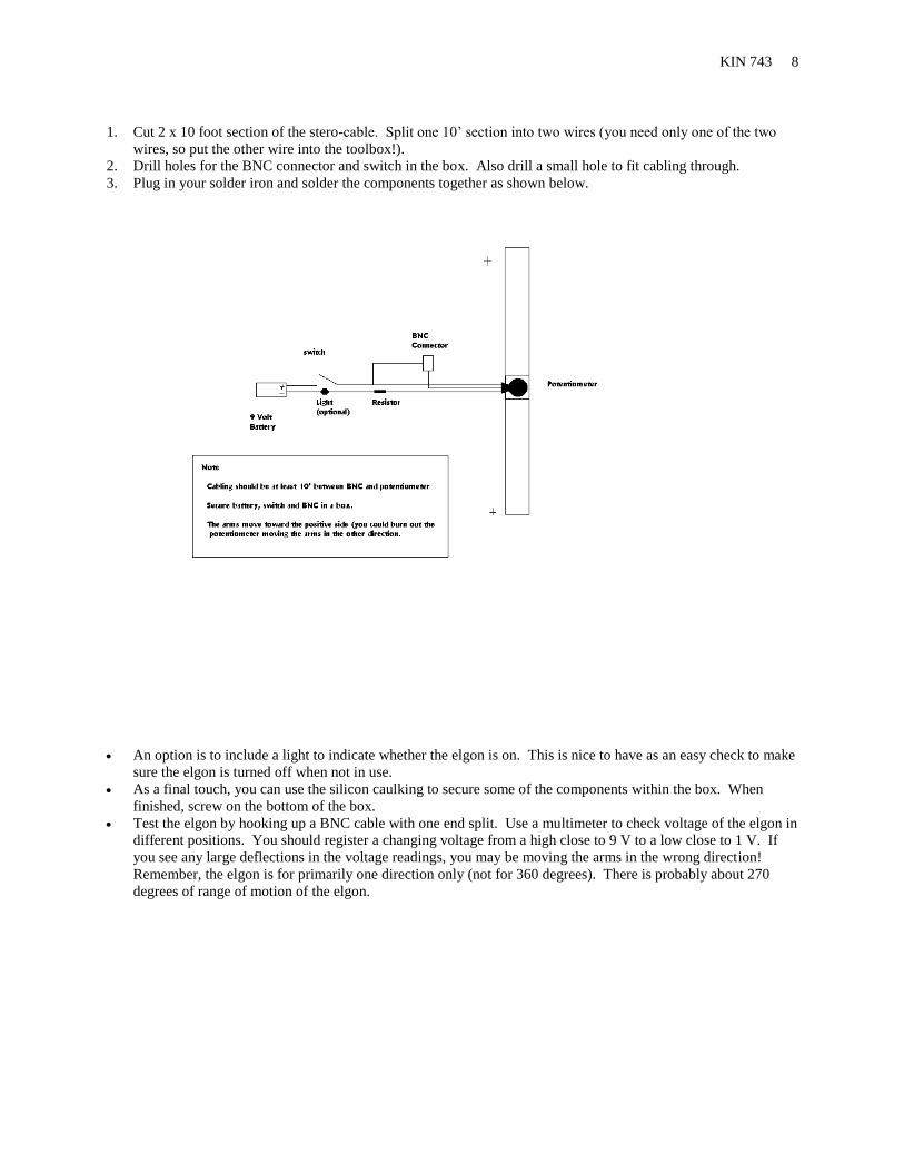
How to make an electrogoniometer
An electrogoniometer (elgon) is used to quantify angular position. The elgon consists of a potentiometer hooked up
to a 9 V battery. The variable resistor is also hooked up to a BNC connector, which allows for connecting the elgon
to an A/D board (e.g. APAS). If done correctly, the voltage output from the BNC will vary depending on the
position of the elgon arms. A conversion factor can be calculated to determine the voltage per degree. Although
this elgon will allow for a good degree of hyperextension, the elgon should not be used for 360 degree revolutions,
as you may damage the potentiometer.
Tools needed:
Soldering iron
Solder
Clippers
9 V Battery
Super Glue
Silicon caulking
Electric tape
File
Electric Drill
Hacksaw
Equipment needed for elgon:
Potentiometer (‘pot’)
Resistor
10’ stero-cable
BNC male connector
9 V Battery clip
On-off switch
Project box
2 x goniometer arms (Plexiglass)
light (optional)
Construction of electrogoniometer arms.
1. Purchase a sheet of plexiglass from a hardware store (cost is less than $10). Cut two straight pieces
approximately 1” x 12” – or to the size that works best for your situation. File edges smooth.
2. Take a marker and mark 6/8” from the end of one arm. This point will be “Hole 1” and will be the axis of
rotation of the goniometer.
3. Mark another point (Hole 2) 9/8” from the same end used in #2.
4. Drill a ¼ inch diameter hole for Hole 1 (big enough for potentiometer post).
5. Drill a 1/8” diameter hole for Hole 2.
6. Use the hacksaw and cut the post of the potentiometer flush with screw threads. Be careful not to damage the
threads.
7. Remove cap from potentiometer by loosening the four tabs.
8. Fit the post through the drilled hole. Fit the metal tab in Hole 2 and secure the potentiometer with the washer
and nut. The potentiometer posts should be on one side of the arm. This side will be the useable side of the
goniometer.
9. Hold the elgon arm such that the moveable portion of the pot is topside (nut and washer on the down side).
Position the large tab near the end of the elgon arm. Lay the 2nd elgon arm over the pot and mark where to cut
openings for the two tabs.
10. Using the 1/8” drill bit, drill out marks for the circle and straight tabs (marked in #9).
At this point, you should have the pot secured between two arms. Use the super glue and fix the pot board to the
metal casing (note that the cap usually holds the board and metal casing together, but we aren’t using the cap!).
Next, super glue the top arm to the pot.
The next steps are for wiring the pot.
KIN 743 8
1. Cut 2 x 10 foot section of the stero-cable. Split one 10’ section into two wires (you need only one of the two
wires, so put the other wire into the toolbox!).
2. Drill holes for the BNC connector and switch in the box. Also drill a small hole to fit cabling through.
3. Plug in your solder iron and solder the components together as shown below.
An option is to include a light to indicate whether the elgon is on. This is nice to have as an easy check to make
sure the elgon is turned off when not in use.
As a final touch, you can use the silicon caulking to secure some of the components within the box. When
finished, screw on the bottom of the box.
Test the elgon by hooking up a BNC cable with one end split. Use a multimeter to check voltage of the elgon in
different positions. You should register a changing voltage from a high close to 9 V to a low close to 1 V. If
you see any large deflections in the voltage readings, you may be moving the arms in the wrong direction!
Remember, the elgon is for primarily one direction only (not for 360 degrees). There is probably about 270
degrees of range of motion of the elgon.

KIN 743 9
Sampling Rate
Sampling Rate
Frequency of sampling analog signal.
Purpose: Best representation of analog signal that is cost effective.
Cost effective:
High speed data acquisition systems are expensive
30 Hz vs. 200 Hz vs. 1000 Hz kinematic system
Computing equipment (e.g., storage of data)
Film, video, etc.
Analysis time increases (personnel cost)
“Best” representation
Qualitatively similar digital and analog pattern (time domain analysis).
Frequency representation of digital and analog signals is similar.
Frequency domain
Sine wave basics
Amplitude, frequency, period, cycle
Superposition: Addition of sine waves
Excell chart illustrating sine wave basics
Sampling theorem
The analog signal can be reconstructed if the digital signal is sampled at twice the highest
frequency present in the analog signal.
Nyquist frequency: The frequency equal to twice the highest frequency present in the analog
signal.
Alaising error: False frequencies present in digital signal.
Minimum rate defined by sampling theorem.
1000 Hz for GRF data
500 Hz for EMG data
100 Hz for rear foot motion
30-200 Hz for most human motion (depending on question)
Maximum rate defined by experience.
Aliasing example using MATLAB

KIN 743 10
Electric Circuit Basics
I = V/R
Types of circuits
Series: Current must flow through each component.
Rt = R1 + R2 + R3 + … + Rn
Vt = V1 + V2 + V3 + … + Vn
It = I1 = I2 = I3 = … = In
Parallel: Current can flow through one component without flowing through another.
1/Rt = 1/R1 + 1/R2 + 1/R3 + … + 1/Rn
It = I1 + I2 + I3 + … + In
Vt = V1 = V2 = V3 = … = Vn
Cathode: Negative terminal
Anode: Positive terminal
Circuit components
Battery: Power source
Resistor: limits current
Variable resistors
Potentiometer
Photoresistor
Light source
LED: narrow wavelength range
Incandescent: many wavelengths
Switch
Pushbutton
Normally open
Normally closed
Temporary
Magnetic: also called a relay since it is closed due to electromagnetic field.
Mercury
Toggle
Other
Diode: Permits flow in a specified direction
Permits flow only when threshold is reached
If current is excessive, the diode will burn out
Reverse voltages can burn a diode out
LED: Light emitting diode
Light is directly proportional to current (I = V/R)
Protect them with resistors in series
Rs = (supply voltage - LED voltage)/LED current
Where LED voltage and LED current are specified
The cathode is on the ‘flat’ side of the LED

KIN 743 11
The Camera
Speed of Light: 3 x 10⁸ m/s in a vacuum. The actual speed is dependent on the material passing through. For
example, in water, the speed of light is 2.25 x 10⁸ m/s.
Refraction: The bending of light when passing from one media to another. When light rays pass into a media where
the speed of light is reduced, light rays will bend toward the normal. When light rays pass from a media where the
speed of light is lower than another media the light ray will bend away from the normal.
Lens
Convex
Concave
Converging
Diverging
Focal point: The point where light rays converge.
Focal Length: The distance the focal point is from the center of the lens.
Short focal lengths increase angle of view (e.g., wide angle lens, f=28 mm)
Normal, similar to eye (e.g., 50 mm lens)
Long focal lengths have a narrow angle of view and magnify the image size (e.g., telephoto lens,
e.g., f=200 mm). Height of object is proportional to the image distance.
Lens equations:
h
h
d
d
f d d
mh
h
d
d
where
h image height
h object height
d image dis ce
d object dis ce
f focal length
m magnification
i
o
i
o
o i
i
o
i
o
i
o
i
o
1 1 1
tan
tan
For example, consider an object 20 cm in height that is 2 m from the center of a f=50mm lens. What would be the
image height?
Answer: 5 mm

KIN 743 12
Camera
Focus ring: Moves the lens closer to or further away from film (i.e., adjusts di)
Shutter-speed: The length of time the shutter is open (e.g., 1 s to 1/1000 s)
Faster movements require higher shutter speeds to prevent blurring of image.
F-stop (a.k.a. aperture, iris): Regulates the amount of light that reaches the film.
f stopf
D
or
Df
f stop
f stop camera setting
f focal length
D diameter of opening
For example, a 28 mm lens set at an f-stop of 2.8 has a diameter of 10 mm
A 50 mm lens set at an f-stop of 2.8 has a diameter of 17.8 mm
Sometimes the f-stop is referred to as the “speed” of the lens. The faster the lens, the greater the
diameter of the aperture. The advantage of a fast lens is that lower light is required for a good picture.
The disadvantage is that more light is passed through the thinner edges of the lens. The effect of
imperfections of lenses will be more apparent in these thin regions.
Circle of confusion: Some objects in focus, others are not. Focus either on close objects, far objects, or
in between so that some close and some far objects are in focus.
Depth of field: range in which circle of confusion is small (i.e., range in which objects are in focus).
A function of f-stop. The smaller the lens opening, the smaller the circles of confusion and the
greater the depth of field.
Advantage of increasing depth of field: increased ‘in-focus’ range.
The disadvantage is that more light is needed since f-stop is small.
Video Camera
CCD: Charge-Coupled Device. This is the transducer that changes light rays into electronic signals
which are recorded on VHS tape. High-quality cameras will most likely incorporate multiple CCD.
Pixels: picture elements. The CCD contains a specific array of pixels. The entire array is analogous to
the film plate in a 35mm camera. Information is stored and read out line by line.
There are two standards for scanning and displaying video signals: NTSC and ATSC.
NTSC: National Television System Committee.
Primary standard in use
The video image contains frames and lines.
30 frames per second
525 lines per frame (actually, 480 are used, with 640 pixels per line)
Odd lines are scanned in 1/60 of a second
Even lines are scanned in 1/60 of a second
1/60 + 1/60 = 1/30
Why?
In early days of TV, the glow of the phosphorescent material in TV would be lost easily.
Transmitting data in this way could be done in the 6 MHz bandwith assigned to TV stations.
ATSC: Advanced Television System Committee
Developed standards for HDTV: High-definition TV
Our TV’s use an aspect ratio of 4:3, HDTV uses 16:9
Increased the number of lines to improve picture resolution (720 lines by 1280 pixels per line)

KIN 743 13
Resolution: the amount of detail a camera can reproduce. Reported in horizontal resolution.
Single CCD camera: 250 lines of resolution
Multiple CCD camera: 600 lines of resolution
But, pictures will be produced at 525 lines.
Recorder
VHS: Video Home System
Records signal at 250-300 lines of resolution
S-VHS (super VHS) increases resolution to 400 lines
The video tape is used to record the video signal (no-duh.). This is done through ‘heads’ positioned on
a drum. The heads are used to record the electrical signal onto the tape through a scanning process
resulting in slanting tracks on the video tape.
The tracks contain video information.
Audio information is contained in an audio track located below the video tracks.
Each track contains information for one field (i.e., 262.5 lines – odd or even).
Errors
Perspective error: When an object moves out of the photographic plane.
Parallax error: Error in location of object based on discrepancy of point of view.
Digitizer error (e.g., selection of centroid)
Camera movement
Calibration errors (e.g., object size, location in photographic plane)
Error in identifying anatomical landmarks
Types of Kinematic instrumentation:
Video
Film
Optoelectric
Electromagnetic
Some systems have the capability to autodigitize, others (e.g., film) require hand digitizing.

KIN 743 14
Motion Analysis
Motion Analysis is a kinematic system which auto-digitizes reflective images. Kinematic digitization serves the
same function as an A/D board – transform an analog signal to digital format. In this case, the digital format
consists of (x,y) coordinates.
When using Motion Analysis, retro-reflective markers are typically used and placed on specific anatomical
landmarks. Retro-reflective markers are used (instead of bike-reflectors) to minimize defraction of light off the
reflective surface. The disadvantage of using retro-reflectors is that the light source needs to be placed in line with
the camera. We will also experiment with using LED light sources instead of retro-reflectors due to laboratory
lighting environment. Do not confuse our use of LEDs with active digitizing systems, which locate and track active
markers (e.g., Selspot).
There are three major steps to digitizing using MA:
1. System setup (e.g., lighting, camera set up, calibration)
2. Collecting data (e.g., VP110, unlvgo.ev)
3. Processing data via QB4.5
1. System setup
Reflector Marker selection
Size of marker depends on image being digitized.
Typically, when digitizing the lower extremity during locomotion or jump-landing, markers
should be no larger than a quarter.
Ample light to reflect markers without distorting markers
Set the camera back as far as possible and zoom in.
Set the f-stop to the largest number (i.e., smallest diameter).
Familiarize yourself with the VP110 processor controls.
Once you have a satisfactory setup, record the VP threshold. Then, working in DOS, change the
directory that you are going to work in and type ‘ev’. Prior to working in this directory, make sure you
have the file ‘unlvgo.ev’ in the directory. For now, let’s all work in the c:\KIN743 directory.
2. Collecting data
Two programs can be used to operate Motion Analysis: EV and MEV.
EV: one camera mode
MEV: two camera mode
The EV mode allows you to operate Motion Analysis through specific commands or through batch
programs.
Unlvgo.ev is a specific EV program to collect digitized data. Note that when using MA, there is no
video record, only digitized coordinates.
Upon successful collection, you should have a file *.bk1 that should be copied to disk.
For each camera setup (and each subject), you should collect a horizontal and vertical reference frame.
3. Processing digitized data
Each *.bk1 file contains x,y coordinates in pixels per path, with (0,0) set at the top left corner of the
image.
The next step involves editing the *.bk1 file to delete errant paths and/or join fragmented paths. This
is done through QuickBasic 4.5 program called UNLVedit.bat

KIN 743 15
Video analysis of motion
Introduction
- Why video tape?
- hard copy of motion
- allows quantifying motion
- video games
- What should be video taped?
- any motion you want to quantify
- What are the advantages of high speed video (>100Hz)?
- smaller time increments/more information
- discrete events can be better defined (ball contact - blurr)
- Conversion of Hz to time interval
- Hz = frames/sec (sec = frames/Hz)
ex: 30 Hz camera: each frame = 1/30th s
200 Hz : each frame = 1/200 s
Subject set up
- reflective markers (assuming that the areas that we are marking are the actual joint center and
that skin movement is negligible)
- same material as on bicycle, clothing, etc.; thus, cover up other reflective markers (ie shoe)
- size of marker and why this is important during digitizing
- blending
- size: optimize to reduce blending error but maximize accuracy
- location of markers are points in space: x,y
- each marker (for this lab) is a joint center/axis of rotation.
- What markers will we need to analyze walking/running?
- Markers needed to calculate joint angles:
1. shoulder: greater tuberosity and acromium process
2. greater trochanter
3. knee: lateral epicondyle of femur and condyle of tibia
4. heel (with shoe): calcaneus
5. malleolus
6. 5th metatarsal
Equipment orientation
- procedures for camera
- camera placed strategically to optimally view complete phase of motion.
- level camera in two planes, and check to make sure camera is perpendicular to field of motion.
- camera as far back using zoom in
- reduces error: increases image size in center of lens
Possible problems with using video analysis:
- error in set up
- image not large enough (data not able to be obtained)
- image not centered in field of vision
(some error will result due to image being refracted through outlying area of lens as well
as viewing perspective error off outlying area of screen)
- error due to reflective markers
- validity of placement
- reliability of placement
- movement of marker due to skin, shoe, ?
- blending of marker (two markers too close!)
- bad marker (not circular)
- excessive/poor lighting

KIN 743 16
Smoothing Data
Every data set analyzed contains noise. In general, the assumptions of noise are:
The frequency content of noise is considered high.
The amplitude of noise is low.
There are many techniques used to smooth data. Some of the techniques used include:
Moving average. For a given data set, a new data set is created by calculating a moving average of the raw
data. For example, a new data point (i) could be created as the average of n-1, n, n+1.
3 point 5 point
Frame time x vx ax Smoothed v a smoothed v a
73 0.067 2.946
74 0.083 2.982 1.64 2.977
75 0.100 3.001 1.42 -8.30 3.004 1.48 3.00
76 0.117 3.029 1.37 -16.27 3.026 1.22 -11.20 3.02 1.27
77 0.133 3.047 0.88 -9.01 3.045 1.10 -2.77 3.04 1.23 0.0
78 0.150 3.058 1.07 16.96 3.063 1.13 8.24 3.06 1.28 1.1
79 0.167 3.082 1.44 16.78 3.082 1.38 10.32 3.09 1.27 2.5
80 0.183 3.107 1.63 -2.77 3.108 1.47 1.56 3.11 1.36 5.5
81 0.200 3.137 1.35 -9.34 3.131 1.43 -2.13 3.13 1.45
82 0.217 3.151 1.31 5.71 3.156 1.40 3.16
83 0.233 3.180 1.54 3.178
84 0.250 3.203
Fourier Smoothing. Signals can be represented by the summation of sine waves of varying
frequency: time to complete a cycle
amplitude: height of sine wave
Steps to Fourier Smoothing include
1. Completing a Fast Fourier Transformation (FFT). That is, calculating amplitudes of frequencies that
estimate the raw signal.
2. Identifying cutoff frequency.
3. “resetting” amplitudes of unwanted frequencies (i.e. high) to zero.
4. Calculating in inverse transformation.
Band-pass. The amplitudes of a band of frequencies are unchanged. For example, it may be desired to have
only frequencies between 3-10 Hz analyzed.
Notch filter. The amplitudes of a band of frequencies are changed. For example, it may be desired to get rid of
powerline (60 Hz) noise.
High Pass. Frequencies above a specified cutoff frequency are passed through the filter (e.g. EMG).
Low Pass. Frequencies below a specified cutoff frequency are passed through the filter (e.g. Kinematic data).
Polynomial. Data can be fit with a polynomial function of degree n of the following form:
X(t) = a0 + a1t + a2t2 + a3t3 + … + an-1tn-1 + antn
EXCELL users: select data series; ‘chart – add trendline – polynomial (2) – show equation’
MATLAB users: [p,s]=polyfit(x,y,n);
smooth_y=polyval(p,x);
%where x = time
% y = vertical displacement
% n = polynomial degree (2nd for projectile motion)

KIN 743 17
Digital Filtering. This is a form of moving average, but a system of sophisticated weights per row is used.
n = fc/fs
where n = cutoff to sample frequency ratio
fc = cutoff frequency (Hz)
fs = sample frequency (Hz)
[for MATLAB users: n = 2(fc/fs)]
c=tan(n)
where c = normalized cutoff frequency
K1 = c(20.5) Butterworth filter
K1 = 2c Critically damped filter
K2 = c2
a0 = K2/(1+K1+K2)
a1 = 2ao
a2 = ao
K3 = 2a0/K2
b1 = -2a0+K3
b2 = 1-2a0-K3
x’(i)= a0 x(i)+ a1(x(i-1))+ a2(x(i-2))+b1(x’(i-1))+b2(x’(i-2))
EXCELL Example
A B C
1 0.067 2.946 2.946
2 0.083 2.982 2.982
3 0.100 3.001 = a0B(3)+ a1B(2)+ a2B(1)+b1C(2)+b2C(1)
4 0.117 3.029
5 0.133 3.047
6 0.150 3.058
7 0.167 3.082
8 0.183 3.107
9 0.200 3.137
10 0.217 3.151
11 0.233 3.180
12 0.250 3.203

KIN 743 18
3D Calibration
The Problem: Calculate 3D coordinates from 2D image plane.
Each point in space can be represented by a unique set of x,y,z coordinates.
Each point on an image can be represented by a unique set of x,y coordinates.
By combining multiple camera views of a point in space, 3D coordinates can be calculated.
The most common methods to transform 2D to 3D includes:
- DLT: Abdel-Aziz & Karara (1971)
- MDLT: Hatze (1988)
- DNLT: Chen (1994)
- NLT: Dapena (1982)
DLT: Uses a set of known spatial coordinates to determine internal and external camera parameters.
Internal Parameters: lens distortion, camera distance from point
External Parameters: Orientation of camera (relative to field of view and to each camera)
x + x + x = (L1X + L2Y + L3Z+ L4)/(L9X + L10Y + L11Z + 1)
y + y + y = (L5X + L6Y + L7Z + L8)/(L9X + L10Y + L11Z + 1)
x,y image coordinates
X,Y,Z spatial coordinates
x, y random digitizing errors
x, y non-linear systematic errors
L1-L11 camera parameters
Required: 6 control points (12 equations).
Recommended: 20-30 control points.
Advantages: accurate within calibration volume.
Disadvantages: accuracy suspect when extrapolating outside of calibration volume.
NLT: Uses reference frame to calculate internal parameters.
Uses control object of unknown shape, but with at least one known length, to calculate external parameters.
Note: Peak requires the user to select a camera - the camera internal parameters have been calculated by
Peak, and therefore the correct camera must be selected.
Required: Reference frame, wand.
Advantages: Able to calibrate a large volume of space without the need of construction a large
calibration cube.
If extrapolation of data outside the calibrated volume is required, the NLT is more
accurate than the DLT.
Disadvantages: Less accurate within the calibrated space compared to the DLT.
For fun reading: Chen, L., Armstrong, C.W., & Raftopoulos, D.D. (1994). JOB 27(4), 493-500.
Dapena, J., Harman, E.A., & Miller, J.A. (1982). JOB 15(1), 11-20.
Dapena, J. (1985). JOB 18(2), 163.
Hatze, H. (1988). JOB 21(7), 533-538.
Henrichs, R.N., & McLean, S.P. (1995). JOB 28(10), 1219-1224.
Kennedy, P.W., Wright, D.L., & Smith, G.A. (1989). IJSB 5(4), 457-460.
Miller, N.R., Shapiro, R., & McLaughlin, T.M. (1980). JOB 13(7), 535-548.

KIN 743 19
Joint Moments
Torque: The tendency of a force to cause rotation. T=Fd
Torque = Moment
Units: Nm
Forward Dynamics: Given segment accelerations, position, velocity and joint moments can be calculated.
Inverse Dynamics: Given position vs. time data, accelerations and joint moments can be calculated.
To solve for joint moments, the following data are required:
Anthropometrics
Kinematics
Kinetics
Anthropometrics
Segment masses
Segment COM
Segment Io
Kinetics
Fy
Fz
COP
Kinematics
for foot, leg, thigh
ax for COM of each segment
ay for COM of each segment
(x,y) coordinates for each joint
Assumptions of a rigid link segment model
Mass and length of each segment are constant.
COM is a fixed point within a segment.
Io is moment of inertia about COM and is fixed.
Steps to inverse dynamic approach
1. Record kinematic and kinetic data concurrently.
2. Record COP to identify location of GRF relative to foot.
3. Calculate segment accelerations in x and y directions.
4. Calculate segment angular velocities.
5. Calculate segment masses and moment of inertias
6. Use equations
Equations for inverse dynamics approach
Fx = max
Fy = may
T = I

KIN 743 20
Moment of Inertia represents the resistance to change angular motion about the center of mass.
Io = m2 units: kgm2
= Radius of Gyration = (coefficient)(segment length)
Io = moment of inertia about segment COM
l = segment length in meters
Segment defined Weight
%BW
COM
%l /l
Head-Arms-Trunk Greater-Trochanter to
Glenohurmeral joint
0.678 0.626 0.496
Head and neck C7-T1 to Ear canal 0.081 1.000 0.495
Upper Arm Glenohumeral axis to Elbow axis 0.028 0.436 0.322
Forearm Glenohumeral axis to Ulnar Styloid 0.016 0.430 0.303
Hand Wrist axis to Knuckle middle finger 0.006 0.506 0.297
Trunk Greater Trochanter to
Glenohumeral joint
0.497 0.500
Thigh Greater Trochanter to
Knee joint approximation
0.100 0.433 0.323
Leg Knee joint appox. To
Lateral malleolus
0.0465 0.433 0.302
Foot Lat. Malleolus to
Head of 5th metatarsal
0.0145 0.50 0.475

KIN 743 21
unknowns
Note: for the foot segment the distal
moment (Md) is 0, the distal forces (Rdx and
Rdy) are the ground reaction forces and the
distal joint location (dx and dy) is at the
center of pressure.
General Equations (Courtesy of Dr. Tim Derrick, Iowa State)
Proximal Reaction Force (x) (Rdx for the foot is the horizontal GRF)
Rpx = max - Rdx
Proximal Reaction Force (y) (Rdy for the foot is the vertical GRF)
Rpy = may - Rdy – mg
Proximal Moment (Md for the foot is zero)
Mp = I – Md – (Rdx*d1) – (Rdy*d2) – (Rpx*d3) – (Rpy*d4)
d1 = CMy - dy
d2 = dx - CMx
d3 = CMy - py
d4 = px - CMx
proximal moment Mp
proximal force x Rpx
proximal force y Rpy
distal moment Md
distal force x Rdx
distal force y Rdy
CM acceleration x ax
CM acceleration y ay
angular acceleration
mass m
moment of inertia I
proximal joint x px
proximal joint y py
CM x CMx
CM y CMy
distal joint x dx
distal joint y dy
gravity g = -9.81
d4
d3
d2
d1 Center of mass
(CM)

KIN 743 22
Free Body Diagram
Fx
m ax
Fy
m ay
M I
Rdyy
Rpy
Mp
Rpx
ay
ax
mg
I
Rdx Md
LEGEND
R reaction force
M moment
I moment of inertia
m mass of segment
g gravitational constant
a linear acceleration
angular acceleration
d distal end of segment
p proximal end of segment
x,y vector directions

KIN 743 23
Sample Joint Moment Calculations
Frame 11 – Ankle joint moment
R1x + GRFx = max
R1x = max - GRFx
R1x = 1.16kg * -.90m•s-2 - (-149.96N)
R1x = 148.92N
R1y + GRFy + mg = may
R1y = may - GRFy - mg
R1y = (1.16kg * 2.25m•s-2) - 878.73N - (1.16kg * -9.81m•s-2)
R1y = -864.74N
M1 + M(R1x) + M(R1y) + M(GRFx) + M(GRFy) = I
M1 = I - M(GRFx) - M(GRFy) - M(R1x) - M(R1y)
M1 = (.009684kg•m2 * 12.18rad•s-2) - (-149.96N * .061m) - ( 878.73N * -.0737m) - (148.92N*-.049m) - (-864.74N
*-.081m)
M1 = .12N•m + 9.15N•m + 64.76N•m + 7.30N•m – 70.04N•m
M1 = 11.29N•m
- M1 is positive indicating a CCW moment
GRFx = -149.96 N
GRFy = 878.73 N
ax = -0.9 m•s-2
ay = 2.25 m•s-2
= 12.18 rad•s-2
m = 1.16 kg Icm = .009684 kg•m2
x y
ankle .849 .110 cm .930 .061
COP .8563 0
GRFx
GRFy
R1x M1
mg
R1y
ay
ax
FOOT SEGMENT

KIN 743 24
Frame 11 – Knee joint moment
R2x + R1x = max
R2x = max - Rlx
R2x = (3.72kg * -4.47m•s-2) – (-148.92N)
R2x = 132.29N
R2y + Rly + mg = may
R2y = may - Rly - mg
R2y = (3.72kg * -.63m•s-2) - (864.74N) - (3.72kg * -9.81m•s-2)
R2y = -830.59N
M2 + M1 + M(R1x) + M(R1y) + M(R2x) + M(R2y) = I
M2 = I - M1 - M(R1x) - M(R1y) - M(R2x) - M(R2y)
M2 = (.0664kg•m2 * 14.01rad•s-2) – (-11.29N•m) - (-148.92N * .249m )
- (864.74N * -.015m ) - (132.29N * -.19m ) - (-830.59N * .012m )
M2 = .93N•m + 11.29N•m + 37.08N•m + 12.97N•m + 25.14N•m + 9.97N•m
M2 = 97.37N•m
- M2 is positive indicating a CCW
M1 = -11.29 N•m
R1x = -148.92 N
R1y = 864.74 N
ax = -4.47 m•s-2
ay = -0.63 m•s-2
= 14.01 rad•s-2
m = 3.72 kg Icm = .0664 kg•m2
x y
knee .876 .549 cm .864 .359
ankle .849 .110
LEG SEGMENT
R’1x M’1
R’1y
mg
ay
ax
R2x M2
R2y
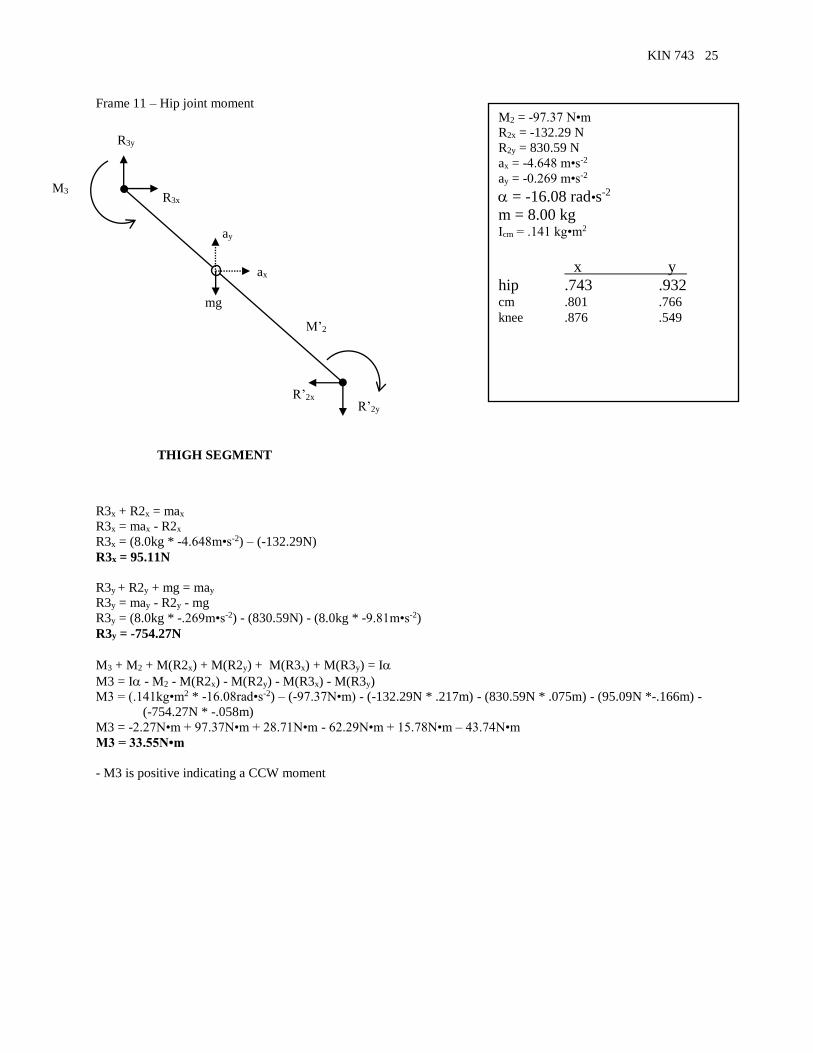
KIN 743 25
M2 = -97.37 N•m
R2x = -132.29 N
R2y = 830.59 N
ax = -4.648 m•s-2
ay = -0.269 m•s-2
= -16.08 rad•s-2
m = 8.00 kg Icm = .141 kg•m2
x y
hip .743 .932 cm .801 .766
knee .876 .549
Frame 11 – Hip joint moment
R3x + R2x = max
R3x = max - R2x
R3x = (8.0kg * -4.648m•s-2) – (-132.29N)
R3x = 95.11N
R3y + R2y + mg = may
R3y = may - R2y - mg
R3y = (8.0kg * -.269m•s-2) - (830.59N) - (8.0kg * -9.81m•s-2)
R3y = -754.27N
M3 + M2 + M(R2x) + M(R2y) + M(R3x) + M(R3y) = I
M3 = I - M2 - M(R2x) - M(R2y) - M(R3x) - M(R3y)
M3 = (.141kg•m2 * -16.08rad•s-2) – (-97.37N•m) - (-132.29N * .217m) - (830.59N * .075m) - (95.09N *-.166m) -
(-754.27N * -.058m)
M3 = -2.27N•m + 97.37N•m + 28.71N•m - 62.29N•m + 15.78N•m – 43.74N•m
M3 = 33.55N•m
- M3 is positive indicating a CCW moment
THIGH SEGMENT
R’2x
M’2
R’2y
mg
ay
ax
R3x M3
R3y

KIN 743 26
Accelerometers
Acceleration:
Rate of change of velocity.
Direction of acceleration indicates the slope of the velocity vs. time plot.
Whether velocity is speeding-up or slowing-down depends on initial velocity.
Direction of motion is given through velocity information.
Techniques to measure acceleration:
Video analysis
Record position vs. time, calculate 2nd derivative.
Force plate
Newton’s 2nd law: F=ma
Accelerometer
Accelerometers
Consists of:
Mass
Transducer material
Piezoelectric crystal material
Strain gauges
Ceramics
Amplifier
Piezoelectric crystal
This material is sensitive to forces placed upon it. When a force acts on the crystal, the material
changes its electric properties. The Kistler force plate also uses piezoelectric crystals. Most
accelerometers do not measure constant acceleration conditions – like freefall or standing weight. This
information is found in accelerometer specifications that identify frequency response of
accelerometers. If the frequency response includes zero, then it measures constant acceleration.
Sensitivity
100 mV/g = 1 g/100 mV = 0.01 g/V
1000 mV/g = 1 g/1000 mV = 0.001 g/V
Accelerometer sensitive axis
Uniaxial
Triaxial
Compression vs. shear
Using accelerometers in human movements
Surface mounted accelerometers
Bone mounted accelerometers
Factors affecting surface mounted acceleration
Rate of change of velocity.
Accelerometer mass (not mass component per se, but total accelerometer mass).
Soft tissue between accelerometer and bone.
Orientation of sensitive axis relative to gravity.
Angular motion (Centripetal acceleration = vT2/r = r2).
Amp
Mass
Crystal

KIN 743 27
Advantages of Accelerometry
Disadvantages
Can record accelerations at high sample rates. An accelerometer is needed for each segment of interest.
Accelerations can be continuously recorded. Sensitive to attachment procedures.
Suitable for testing impact magnitudes. Attachment procedures could affect human performance
(e.g., too tight attachment).
Representation of segment accelerations. Single sensitive axis changing relative to gravity.
Integration is possible only if vi is known.

KIN 743 28
Impact Testing and Springs
Biomechanic analyses often involve quantifying elastic behavior of a material, object, or person during some
activity. Testing elastic behavior of an object or material often involves impact testing, while testing elastic
behavior of a person during a task involves recording kinetic and kinematic data concurrently.
Elastic: The ability to return to original position.
Pure elastic behavior in not dependent on time, or loading rate. However, the elastic behavior of most materials
(e.g., surfaces, bone, tendon) is dependent on time.
Viscoelastic: The elastic response is dependent on loading rate.
Viscosity: fluid property, a measure of resistance to flow.
Elasticity: material property, a measure of the ability to return to original shape.
A technique used to test viscoelastic properties of an object is to impact test it via impact tester. An impact missile
is dropped on the test surface and recordings of force and displacement are made.
Hysteresis: Same path not taken during loading and unloading.
Hysteresis loop: Represents the energy lost in the collision; or, the energy not returned by the object (dissipated as
heat).
Energy: The capacity to do work.
Potential Energy of position: mgh
Kinetic Energy: ½ mv2
Potential Energy of a spring: ½ kx2
Conservation of Energy: Energy can neither be created nor destroyed. It may only change from one form
to another.
During collisions, energy pre-collision = energy post-collision
Epre = Epost
Load
Deformation
Load
Deformation

KIN 743 29
PEi + KEi = PEf + KEf + Q
At impact: E = KEi
At max deformation: E = PEspring
At point of missile takeoff: E = KEf
Important: KEi KEf (i.e., energy is dissipated)
KEi = KEf + Q
Q: Represents the non-mechanical energy (e.g., heat).
Area of Hysteresis loop = Q: The energy not returned by the material during a collision.
Mass-Spring Model
The amount of deformation of a spring determines the amount of force exerted back by a spring.
F = -kx
The negative sign indicates that the force is always directed back to the equilibrium position of the spring.
To calculate k of an object, apply a force to it and measure the deformation.
How would you calculate lower extremity stiffness while hopping?
In-class Experiments:
1. Calculate the spring stiffness of one of a rubber band.
2. Impact test different materials and calculate the spring stiffness of each material.
Modeling the human body as a spring
Pros
A mass-spring model can be used to predict human movement (e.g., GRF).
A simple model can be used to understand human movements (e.g., hopping, running)
Cons
The human body is not a spring since deformation can occur with no recoil necessary.
The stiffness of the lower extremity stiffness can vary within a cycle (e.g., during the landing phase
during running).
m
m
x

KIN 743 30
Electromyography
Electromyography (EMG): The study of the electrical signal associated with muscle contraction.
A powerful tool to understand human movement. A very powerful tool when used in conjunction with some
other kinematic instrumentation (e.g., elgon).
1. What is being measured?
2. How do you measure EMG?
3. How do you process EMG?
4. What does it mean?
Muscle contraction occurs as a result of:
CNS signal
Transmission of signal to motor end plate via motor neurons
Upon reaching post-synaptic membrane threshold, signal is transmitted throughout muscle fibers of a
motor unit ( motor neuron and all innervated muscle fibers).
EMG measures the electrical depolarization-repolarization cycle of muscle activation.
Terminology
Motor unit
Muscle fiber action potential
Motor unit action potential (muap)
Synchronization: tendency for different motor units to fire simultaneously.
Motor point: location where smallest external stimulus is needed for muscle contraction (i.e.,
innervation zone).
How to measure:
Goal: quantify muscle activity.
Piezoelectric Contact Sensors
Microphones
Accelerometers
Optical methods
Pressure transducers
Electromyography
The problem: The electrical activity of muscle contraction is small and generally motor units fire
asynchronously. For surface EMGs, the electrical activity must be recorded through subcutaneous fat,
connective tissue (e.g., tendon sheath), skin, electrolyte gel, lead material, wire, amplifier, and finally
computer.
The EMG system must take into account all these factors (and more) when generating the resulting
‘raw’ signal.
Skin resistance: reduce by shaving, abrading, cleaning.
Electrode, electrolyte transition: resistance is a function of material. Electrodes come in all different
styles and materials. The Noraxon system uses a lead that connects to a ‘patch’ that contains
electrolyte gel. If this gel is not good, the lead is no good.
The wires act as antennae (part of ‘system’) that record electrical wilderness signals and may tug on
electrodes and cause movement artifacts.
skin system Amp
EMG

KIN 743 31
Amplifier: This system amplifies the input signal – which may contain noise. Good amplifiers amplify
all frequencies equally, meaning that noise is amplified. Some ways to reduce amplification of noise:
Analog filters (booo for you if you do not know)
CMRR (discussed below).
High pass filters – removes movement artifacts
Low pass filters – removes high-frequency noise
Other analog filters (these are boo for me)
Locate amp as close to muscle surface as practically possible (sometimes boo, sometimes
not).
Some EMG systems include an amp on the electrode (true ‘pre-amp’ systems). Others, such
as the Noraxon have the amp located between the electrode and computer.
EMG basics:
One lead system:
Most EMG systems use a two electrode system to record muscle activity:
Most EMG systems use a third lead as a reference lead to identify noise common to both leads. This
lead is typically placed on an inactive site (e.g., bony landmark).
Common-Mode Rejection
The signal common to both leads is removed through difference between leads (see EMG.xls). This
procedure is referred to as CMR and is completed in the amplifier (i.e., differential amplifier).
A = (b+N) – (c+N) = (b-c)
Therefore, common noise is removed from the signal. Usually, the amplifier’s ability to remove noise
from the signal is reported as the common-mode rejection ratio (CMRR). This value represents the
ratio of noise removed relative to signal amplitude. For example, if the CMRR is 2000:1, then all but
1/2000 of the noise is removed from the signal. Usually, the CMRR is reported in decibels using the
following calculation:
CMRR (dB) = 20log10(ratio)
Therefore, for a 2000:1 CMRR, the dB would be: 20log10(2000) = 66 dB
What is the CMRR of the Noraxon amplifier?
Processing EMG
Remove DC bias. Calculate mean of all data, subtract mean from each data point.
Rectify:
Full wave rectification: absolute value of all EMG values (recommended).
Half wave rectification: analyze positive data only.
V1
V2
V2-V1
T(1) T(n)

KIN 743 32
Lot’s of options at this point
Smooth
Butterworth
Moving window average (recommended)
Used to quantify EMG pattern.
Integrate
IEMG = x(t)/fs (Rectangular integrator)
IEMG = (x(n)+x(n+1))/2fs
Units: mVs
Over a time period (recommended).
Reset after some specified time period (e.g., 50 ms). This is similar to a moving average.
Reset after some specified voltage value (e.g., 50 mV). The number of resets are recorded for
analysis, more resets = more active muscle.
IEMG used to quantify activity of muscle.
Average EMG
Units: mV
Across some time specified period
Used to quantify activity of muscle, normalized to time.
Linear Envelope
Common EMG phrase used to describe the following process:
DC bias removed
Full wave rectification
Low pass filter
Normalization
Since there are a lot of variables that determine magnitude of EMG for a given person, EMG data are
typically normalized to some baseline value. This baseline measure could be:
Maximal voluntary contraction
Quiet record of EMG
Some baseline condition. For example, when comparing EMG across three running speeds,
magnitudes could be normalized to the slowest speed EMG magnitude.
Interpreting EMG
Carlo J. De Luca, 1997. The use of surface electromyography in Biomechanics. Journal of Applied Biomechanics,
13, 135-163.
Electromyography is a seductive muse because it provides easy access to physiological processes that cause the
muscle to generate force, produce movement, and accomplish the countless functions that allow us to interact with
the world around us. The current state of surface electromyography is enigmatic. It provides many important and
useful applications, but it has many limitations that must be understood, considered, and eventually removed so that
the discipline is more scientifically based and less reliant on the art of use. To its detriment, electromyography is
too easy to use and consequently too easy to abuse.
Recommendations
Have subject warm-up prior to instrumenting.
Minimal sample rate = 500 Hz.
Know the software and hardware specifications.
Identify appropriate site. For our lab, that means locate the belly of the muscle and be able to identify fiber
orientation. If you can quantify motor point (i.e., innervation zone), do NOT put leads over this area. Rather
put the leads proximal to the motor point.
Prepare site appropriately. Shave, abrade, clean, repeat. Even if someone presents shaved, abrade and clean.
Reduce skin resistance.
Use ‘good’ leads and/or gel. Do not let gel communicate between leads. Watch for sweat contaminating the
leads.
Place lead centers about 2 cm apart, in line with muscle fibers.
Fix connectors and wire to minimize movement artifact.
Locate and clean site for common ground.

KIN 743 33
In methods, identify clearly processing steps.
Prior to collecting data, know what you are going to do with EMG data (e.g., analyze iEMG, average EMG,
patterns, …).
Avoid between subject comparisons (use within-subjects design).
Avoid between muscle comparisons of magnitude.
Avoid between day comparisons.
Report amplifier specs (gain, CMRR, any filtering, differential lead).
Report processing steps (DC bias, full-wave rectification, …).
Use appropriate units (iEMG = mVs, average EMG = mV).

KIN 743 34
Isokinetic Dynamometer An Isokinetic Dynamometer is a fancy word identifying an instrument that allows for measuring forces during same
speed movements. Remember the different types of contractions from your Exercise Physiology studies:
Isokinetic: Contractions where angular speed is constant.
Isometric: Contraction where distance is constant.
Concentric: Contraction where muscle shortens.
Eccentric: Contraction where muscle lengthens (but it’s trying to shorten!)
There are several manufacturers of Isokinetic Dynamometers:
KinCom (our lab has one)
Cybex Orthotron
BioDex
Each of the instruments allows for measuring force exerted by the user against a pad. Some of the machines report
the user in Torque, others in Force. We’ll discuss the difference between torque and force during the section on
Angular Kinetics.
The tester sets a specific angular velocity for the user to use during exercise. The interesting aspect of this type of
machine is that no matter how hard the user pushes against the pad, the angular velocity will not exceed the angular
velocity set by the tester (i.e. isokinetic exercise).
Can you figure out how long it would take to complete a single knee extension exercise through 90 degrees (i.e.
angular displacement) with the machine set to 30 degrees/second?
In the lab setting, we use this machine to quantify muscle contractile properties over a range of speeds.
When using the machine, it is important to line up the machine axis of rotation with the anatomical axis of rotation.
That is, if you are setting up a user for knee extension exercise, it is important to line up the knee joint axis with the
machine axis. If you do not appropriately line up the two axes, the user will be rather uncomfortable and at risk of
injury.
Here’s some things to try:
Can you exert the same magnitude of force across a range of angular velocities?
During knee extension exercise, can you exert the same amount of force while sitting vs. lying on your back?
What angular velocity would you need to select in order to test an isometric contraction?
Is there a difference in how much force you can exert near the ends of ROM compared to the midrange of ROM?

KIN 743 35
Energy
Energy: The ability to do work.
Work:
The transfer of energy from one object to another.
The product of the magnitude of force and the distance through which the force acts.
Used to describe what is accomplished by a force.
W = Fd Units: Nm or Joule
Energy cannot be created or destroyed. It may only change from one form to another.
E1 = E2
Energy has to come from somewhere and go somewhere.
Energy is needed to get an object moving
Energy is needs to be dissipated to slow an object down.
Mechanical Energy:
PE: Potential Energy
o Position: PE = mgh
o Spring: PE = ½ kx2
KE: Kinetic Energy
Units: Joule
Power:
The rate at which energy is transformed from one form to another.
The rate at which work is done.
Unit: Work/time = J/s or Watt
Power vs. Energy
What a person can do is not limited only by the total energy required but also the rate at which the energy is
used.
P = W/t = Fd/t = Fv
Angular parameter: P = T
Since power is a measure of the rate of energy being transformed (maybe to heat or some other non-mechanical
form) it is used to calculate ‘Energy Absorbed’ and ‘Energy Generated’ parameters.
Energy Absorbed: T and have the opposite directions.
Energy Generated: T and have the same directions.
Quadriceps eccentric contraction: T is an extensor moment (i.e., negative) is flexion (i.e., positive).