reports tabled between the 2001 and 2004 elections
TRANSCRIPT
A statistical analysis of government responses to committee reports
Reports tabled between the 2001 and 2004 elections
David Monk1 This paper measures the government acceptance of recommendations of parliamentary
committees. Such information is one way in which a committee can demonstrate its
effectiveness. Out of all committee reports where the majority report requested the
government take new action, the sample shows that 63.2 per cent of committee reports
demonstrated a minimum level of effectiveness (at least one recommendation in a report
accepted). The factors that show the strongest statistical correlation with this minimum level
of effectiveness are the type of committee, bipartisanship, the number recommendations,
press coverage and whether it was a terrorism inquiry.
Introduction The requirement for governments to respond to committee reports has existed since the 1970s.
In 1973, the Senate passed a resolution requiring the government to respond to Senate
committee recommendations within three months.2 This followed the Senate creating its
extended committee system in 1970. In 1978, the government made a declaration that it
would respond to committee reports within six months, effectively extending the Senate
system to House and joint committees. The then government reduced this period in 1983 to
three months.3
The government response, if it occurs, is a significant milestone in the life of an inquiry. In it,
the government usually lists what action it plans or has done in respect of each
recommendation. Where the government rejects a recommendation, this usually includes the
reasons why. The House of Representatives Standing Committee on Procedure noted the
importance of the government response. This committee stated that, without some indication
1 A number of people have contributed to this paper in various ways. They include Robyn McClelland and Russell Chafer. 2 The Senate, Standing Orders and other orders of the Senate, September 2006, Resolution expressing opinion of the Senate no. 37. 3 M.E. Aldons, ‘Promise and Performance: An Analysis of Time Taken for Commonwealth Governments to Respond to Reports from Parliamentary Committees’, Legislative Studies, vol. 1, no. 2, p. 20.

2
that the government had at least seriously considered the recommendations in a report, then,
‘The value of the activity becomes questionable’.4
In a related paper in this volume, this author suggests a possible interpretation of the
acceptance of recommendations. Because committees are political entities operating in a
political environment, it is fair to evaluate them by how various groups subjectively react to
their reports. One way of measuring how the government perceives a report is to calculate the
number of recommendations it agrees to implement. This is not a perfect measure. For
example, the government may not meet its commitments. However, as an approximation, or
‘proxy’, of the government’s perception, it is the best we have available that covers policy,
legislation and administration.
Committee reports have various aims and there are a number of diverse groups in the political
system. Therefore, it would be fairer on committees to view the government response as one
way among many for committees to demonstrate their effectiveness. If other groups such as
stakeholders, voters or the legislature favourably perceive a committee report, then the lack of
a government response should not prevent that report from being rated effective. In other
words, a positive government response is a sufficient, but not necessary way for committees
to demonstrate effectiveness.
Collecting the data Notwithstanding the three month requirement, the government can take over three years to
draft and table its response to a committee report. Therefore, the period from which to collect
data needed to be at least three years prior to the project, which commenced in September
2007. This led to the selection of the period between the 2001 and 2004 elections. The Senate
and House registers of committee reports were copied and combined into one master list of
512 reports. A list of random numbers was generated and paired with this master list, giving a
random ordering of reports. The one complication was that joint committees administered in
the Senate are included in both chambers’ registers. Therefore, any House listings of these
reports were skipped; only Senate listings were used. The master list in effect comprised 496
reports.
4 House of Representatives Standing Committee on Procedure, It’s your House: Community Involvement in the

3
The reports were assessed in the order of the random list. To be included in the sample, each
report needed to make a recommendation to the government requiring it to take new action.
Previous studies have noted that committees can word recommendations in a particular way,
making it easy for the government to accept them and inflating the acceptance rate.5
Requiring new action prevents the distorting effect of these recommendations. Therefore,
reports which had no recommendation were excluded from the sample. This meant Senate
estimates reports and the regular Senate inquiries into annual reports were not included. Nor
were the activities of the Senate Standing Committee on Regulations and Ordinances, which
rarely tables reports. It also meant that reports containing single recommendations supporting
proposed government action, such as many reports by the Parliamentary Standing Committee
on Public Works and by Senate legislation committees, were also excluded. In total, 196
reports were examined to generate a sample of 76. The sample comprised 33 joint committee
reports, 20 Senate references and select committee reports, 13 Senate legislation committee
reports and 10 House committee reports. All the reports and government responses were
collected from the Internet.6
Describing and defining the data
Attaching numbers to a flexible, subjective process such as committee reports and the
government response requires a number of decision rules and definitions to ensure that the
data is prepared in a systematic, uniform way. These definitions are listed below, along with
some summary data for the sample. Further information is in the appendix.
Government response
Generally, this was simple to resolve. The government tables in one or both chambers a
document entitled, ‘the government response’. However, this does not occur where a
committee enquires into a bill. In this case, the government’s response is made orally in the
chamber debates. The government was considered to have responded to a report where either
a minister or parliamentary secretary made a statement in Hansard about the government’s
attitude to one or more identifiable recommendations. Out of the 76 reports in the sample, 54
(71.1 per cent) received a government response.
procedures and practices of the House of Representatives and its committees, 1999, p. 66. 5 Malcolm Aldons, ‘Rating the Effectiveness of Parliamentary Committee Reports: The Methodology’, Legislative Studies, vol. 15, no. 1, p. 26. 6 The Parliament’s website is at http://www.aph.gov.au.

4
Acceptance of a recommendation
Often, recognising the acceptance of a recommendation or otherwise by the government is
straightforward. There are some situations, however, where it can be unclear. For instance, the
government might state that it agrees with a recommendation in-principle, but then state it
does not have the resources to implement it. Each individual response to a recommendation
was graded according to the degree of conformity with the committee’s proposal. The
categories are shown in figure one.
Figure 1: Grading of government responses to individual recommendations
Agreed
Partially agreed
Acceptance
Still under examination
Already being done
Agreed in principle
Rejection
Rejected
‘Agreed’ and ‘rejected’ are self-explanatory. ‘Partially agreed’ occurs where a
recommendation has several parts and the government agrees to implement at least one but
not all of them. It can also occur when the government agrees with the idea behind a
recommendation but uses a different method to achieve a similar result. ‘Under examination’
occurs where the government is still considering a recommendation. Given that the
government can take up to several years to respond to a report, it appears fair to count this as
an acceptance. If the government wished to reject such a recommendation, it could do so
quickly. The principle behind making these types of responses acceptances is that the
government has promised new action or at least left open the possibility of it.7
The other three categories are considered rejections because they preclude the government
taking new action. As noted earlier, the category of ‘agreed in-principle’ implies that the
7 Previously supported in Malcolm Aldons, ‘Rating the effectiveness of committee reports: some examples’, Australasian Parliamentary Review, vol. 16, no. 1, p. 55.

5
government will not be taking new action in relation to a recommendation. Sometimes, the
government stated in a response what programs and procedures were already in place. Where
these were implemented before the report was tabled, this counted as a rejection. If it occurred
after tabling, this became an acceptance. The disadvantage of this decision rule is it is
arbitrary. It does not allow for instances of ‘bureaucratic anticipation’ where the government
and the bureaucracy start addressing issues due to committee pressure before a report is
tabled. The advantage of this rule is that it is clear and allows for consistent decision-making
within current limits of information.
These categories are similar to some of those used as headings in government responses.
However, the headings did not always correlate with the content of the response. Therefore,
the categories used here are based on the content of the response, rather than the heading.8
After deciding which recommendations were accepted, an ‘acceptance rate’ was calculated,
which was the percentage of ‘eligible recommendations’ that had been accepted. Eligible
recommendations were defined as those recommendations that were the government’s
responsibility and required new action. Therefore, recommendations directed at the private
sector or independent entities such as the Australian Securities and Investment Commission
were not included. Recommendations for the government to maintain current arrangements,
usually indicated by the word ‘continue’, were also excluded.9 In the sample, the government
accepted at least one recommendation for 48 reports (63.2 per cent). Combining the
acceptance rate across all reports gives an average acceptance rate of 35.2 per cent.
Committee type
Over time, the chambers have changed their committee systems to suit their demands. During
the sample period of 2001-2004, there were four main types of committee: joint, Senate
references and select,10 Senate legislation and House. The Senate introduced the arrangement
of two types of committee in 1994. The convention was for the government to have a majority
8 The variability of headings in government responses has already been noted: Malcolm Aldons, ‘Rating the Effectiveness of Parliamentary Committee Reports: The Methodology’, Legislative Studies, vol. 15, no. 1, p. 30. 9 Id., p. 26 and Malcolm Aldons, ‘Rating the effectiveness of committee reports: some examples’, Australasian Parliamentary Review, vol. 16, no. 1, p. 55. 10 Select committees are technically different to standing committees because they are appointed for the duration of an inquiry, rather than the duration of the Parliament. Otherwise they operate in much the same way because they have the same majority structure and the same sources of referrals. From this point, the text only refers to references committees.

6
on the legislation committees and the opposition to have a majority on the references
committees. A comparison of committees’ source of inquiries and composition during the
sample period is in table one.
Table 1: Comparison of different committee types, 2001-2004
Committee type External referral Self-referral Majority
Joint House, Senate and ministers
Sometimes self-referral within terms of reference
Government
Senate references and select
Senate Select committees may have self-referral within terms of reference
Opposition
Senate legislation Senate Estimates and annual reports Government
House House and ministers Annual reports and Auditor-General reports
Government
Source: Harry Evans, ed., Odgers’ Australian Senate Practice, 11th edition, Department of the Senate, 2004, p. 382. I.C Harris, B.C. Wright, & P.E. Fowler, House of Representatives Practice, 5th edition, Department of the House of Representatives, 2005, pp. 624, 628.
The main point of difference between these committees is that Senate references committees
are the only ones where the opposition has a majority. Since 1972, governments have rarely
held the balance of power in the Senate.11 Within Australia’s institutions of state, there are
few bodies which oppositions can control. Achieving a majority on the floor of the House
delivers that chamber and the whole of the executive to that political party. The one institution
that oppositions have had some measure of control, along with its prestige and resources, is
the Senate. Over time, oppositions have come to use this chamber as a means of promoting
their values and challenging the government. The Senate has become a ‘second bite of the
policy cherry’ for parties that lose the election, or at least are not involved in a majority of
seats in the House.12 Due the ‘invisible hand’ of competition, the opposition’s use of the
Senate to challenge the government brings about democratic outcomes in transparency and a
widened debate. The electorate supports this role in general.13 It also suggests that, on
average, Senate references committees are likely to have lower acceptance rates than other
11 Senator George Brandis, ‘The Australian Senate and Responsible Government’, The University of New South Wales Law School and Gilbert and Tobin Centre of Public Law, 2005 Constitutional Law Conference, pp. 10,16 of 23, http://www.gtcentre.unsw.edu.au/publications/papers/docs/2005/5_GeorgeBrandis.pdf (accessed 9 November 2007). 12 This idea raised in the context of judicial review by Martin Shapiro, ‘Judicial Delegation Doctrines: The US, Britain, and France’, West European Politics, vol. 25, no. 1, p. 179. 13 Senator George Brandis, ‘The Australian Senate and Responsible Government’, The University of New South Wales Law School and Gilbert and Tobin Centre of Public Law, 2005 Constitutional Law Conference, p. 6 of 23, http://www.gtcentre.unsw.edu.au/publications/papers/docs/2005/5_GeorgeBrandis.pdf (accessed 9 November 2007).
7
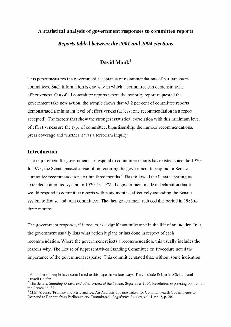
types of committees due to their lack of cooperation with the government. Figure two
demonstrates this.
Figure 2: Average acceptance rates of recommendations by committee type, 2001-2004 (%)
0.0
10.0
20.0
30.0
40.0
50.0
60.0
Joint SenateReferences
SenateLegislation
House Total
Source: A sample of 76 committee reports.
The average acceptance rate for Senate references committees was the lowest at 13.6 per cent.
This suggests that governments have the least use for Senate references committees of all
committee types. It also supports the theory that, on average, oppositions use Senate
references committees for overtly political ends. Governments respond the most favourably to
joint committee reports, which had an average acceptance rate of 54.0 per cent. The most
likely reason for this is the degree of consensus and authority behind these committees.
Firstly, both chambers have agreed to establish joint committees. This means that they have
an innate consensus that no other committee can have. Secondly, they have a great deal of
authority because their membership comprises both Senators and Members.
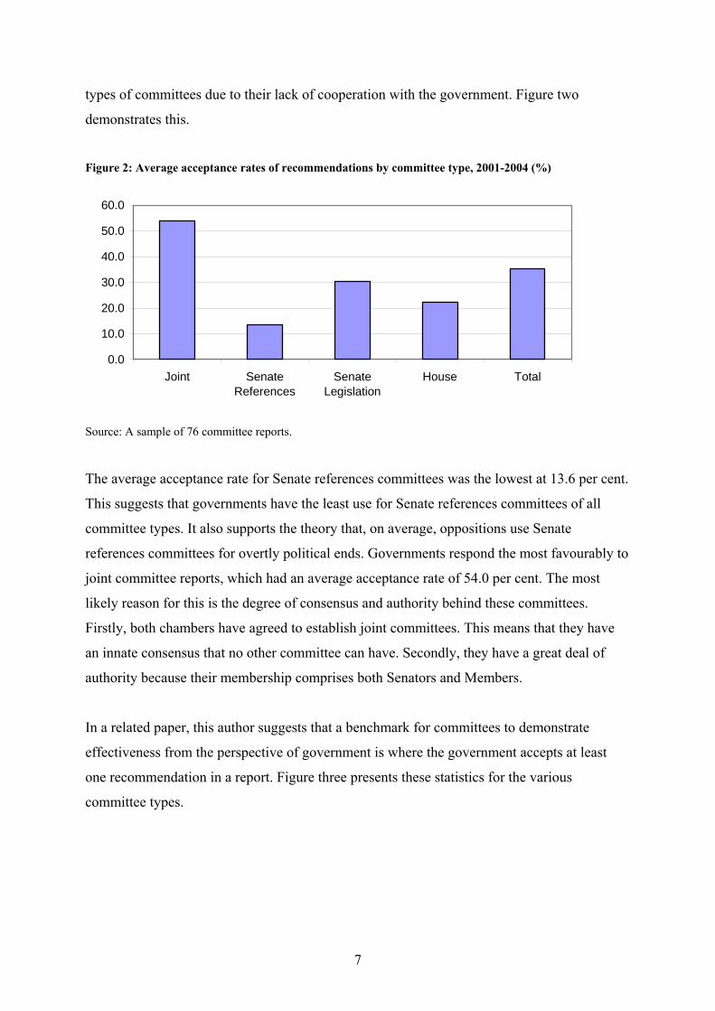
In a related paper, this author suggests that a benchmark for committees to demonstrate
effectiveness from the perspective of government is where the government accepts at least
one recommendation in a report. Figure three presents these statistics for the various
committee types.
8
Figure 3: Proportion of reports with a positive acceptance rate, 2001-2004 (%)
0.010.020.030.040.050.060.070.080.090.0
Joint SenateReferences
SenateLegislation
House Total
Source: A sample of 76 committee reports.
In relation to joint committees, the pattern in figure one is repeated. They have the highest
proportion of reports that, viewed from the perspective of government, demonstrate a
minimum level of effectiveness. However, the pattern in figure one is not repeated in relation
to the other committees. For instance, House committees have a high level of reports (70 per
cent) where at least one recommendation is accepted, but a low overall acceptance rate (22.4
per cent). This means they tend to have a large proportion of reports with a small number of
accepted recommendations. Another example is Senate legislation committees. They are rated
second in figure one (30.5 per cent), but last in figure two (38.5 per cent). This suggests that
governments do not often acknowledge or agree to implement the recommendations of these
committees, but when they do, they accept a high proportion of the recommendations. This
raises the question of whether bills inquiries work differently to other types of inquiries. The
paper uses regressions to test this issue later.
Another way of differentiating committees is that some joint committees are established by an
act of Parliament, rather than by a resolution of both chambers. Examples are the Joint
Committee of Public Accounts and Audit and the Joint Committee on Corporations and
Financial Services. This extra prestige could increase the acceptance rates for these
committees’ reports. Of the 33 reports from joint committees in the sample, 21 come from
committees established by legislation. The regression at the end of the paper tests whether a
legislated function affects the acceptance rate.
9
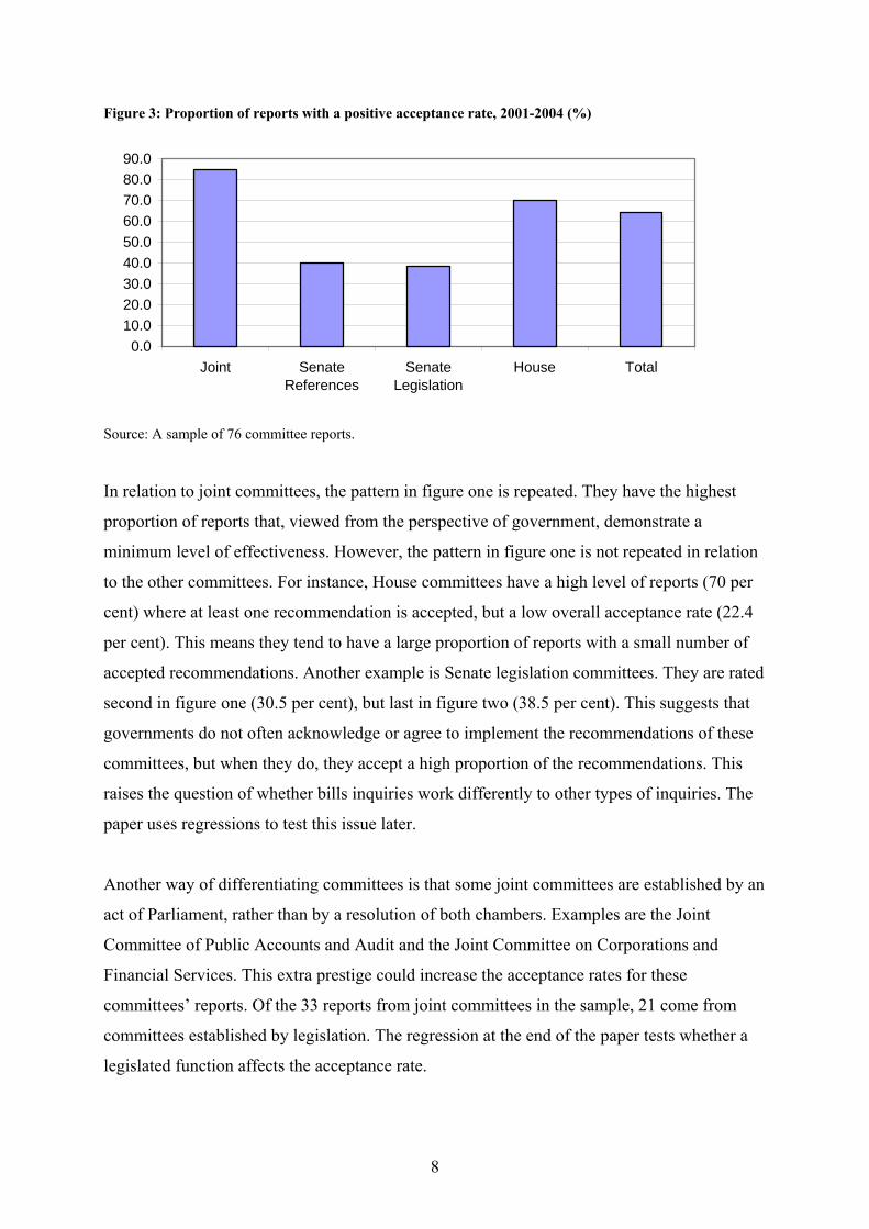
It is also possible to check whether the way in which the government accepts or rejects a
recommendation differs across committee type. Figure four presents the data.
Figure 4: Breakdown of type of government response to recommendations, 2001-2004 (%)
0%
10%
20%
30%
40%
50%
60%
70%
80%
90%
100%
Joint
Senate
Refe
rence
s
Senate
Legis
lation
House
Total
RejectIn-principleAlreadyExaminePartAgreed
Source: A sample of 76 committee reports
This diagram is a more complicated version of figure two. The shaded areas corresponding to
‘examine’, ‘part-agreed’ and ‘agreed’ responses are acceptances and add up to the same
amounts presented in figure two. There are a number of observations to make from the chart.
Firstly, House committees have the highest number of ‘already’ responses. In general, these
responses relate to the recommendations where the government lists a number of actions that
it is already taking. House committees are the only type where the government has exclusive
control of both the reference and the majority. Therefore, there is some evidence that House
committees are conducting low risk inquiries from the government’s perspective. This may
explain why House committees have low acceptance rates but a large number of reports
where the government accepts at least one recommendation.
There are further observations. The short deadline for bills inquiries and the fact that ministers
responded to them during debate in the chamber means that there is little scope for the
government to make ‘already’ or ‘examine’ responses. Therefore, these do not appear for
10
Senate legislation committees. The number of times in total when the government made an
‘examine’ response is low, which suggests that it was not a routine method of avoiding
responding to a report. Therefore, reading an ‘examine’ response as an acceptance appears
appropriate.
Type of inquiry
In his analysis of committee effectiveness, Derek Hawes suggests that the type of inquiry can
affect how the government responds to the report.14 Here, the type of inquiry was
demonstrated in two ways. The first was to select reports that had a contentious subject
matter. During the 40th Parliament, probably the two most contentious issues were terrorism
and immigration. In the sample, there were nine terrorism reports and five immigration
reports. The regressions at the end of the paper tested whether these categories affected the
government response. The expectation would be that their contentious nature would reduce
their acceptance rate.
The second way of viewing the type of inquiry was by what or whom was subject to scrutiny.
The categories were ministerial conduct (three reports),15 administrative (13 reports), bill (20
reports) and policy (40 reports). One theory to be tested is Hawes’ observation that
administrative inquiries are less contentious and have higher acceptance rates.16 Further, the
earlier discussion has suggested that, once the government decides to accept some
recommendations in a bill inquiry, the acceptance rate for that report tends to be high.
In differentiating between administrative and policy reports, one criterion was that
administrative reports tended to focus on how agencies managed themselves.
Recommendations involving new programs, legislation or significant funding were classified
as policy. Where reports had a blend of administrative and policy recommendations, the
classification was based on which sort of recommendations were the most numerous.
14 Derek Hawes, Power on the Back Benches? The growth of select committee influence, School for Advanced Urban Studies, Bristol, 1993, pp. 119-123. 15 Senate Select Committee on Ministerial Discretion in Migration Matters, Report, 2004, Joint Committee on ASIO, ASIS and DSD, Intelligence on Iraq’s weapons of mass destruction, 2003, and Senate Select Committee on a Certain Maritime Incident, Report, 2002. 16 Derek Hawes, Power on the Back Benches? The growth of select committee influence, School for Advanced Urban Studies, Bristol, 1993, pp. 119-123.
11
Bipartisanship
The literature includes significant discussion about the value or otherwise of bipartisanship in
committee work. Bipartisanship is a matter of balance. If committees conduct ‘safe’ inquiries
that are sure to result in bipartisan reports, there is doubt about their relevance. However, if
they conduct very contentious inquiries, they may not be able to agree on the report, giving it
less authority. Some commentators suggest that committees conduct inquiries into areas
where political parties are yet to form their position. This gives committee members more
flexibility in negotiating and increases the chances of a bipartisan report.17
Bipartisan reports are attractive to government. One way of viewing government is as a
seeker of ideas to develop new policy and satisfy the simultaneous demands of those who
fund and support their party and those who allocate power between the political parties
(voters). Governments have close links to their power bases and are well informed about these
demands and interests. However, there is more uncertainty about what policies have support
across the electorate. One source of mainstream policies is bipartisan committee reports.
A bipartisanship index was created to measure rates of bipartisanship. The basis for
calculation is the percentage of the committee members that support the majority report and
do not attach their own additional comments. Where there is no majority report, the index is
the largest percentage of committee members that support an individual report. If some
committee members support the majority report but attach additional comments, this is still
categorised as a ‘dissent’ because the majority report did not meet their needs. If the whole
committee supports the majority report and no member adds their own comments, then the
bipartisanship index for that report is 100. If two members in a six person committee dissent,
then the index will be 66.7. Figure five shows the level of bipartisanship in the sampled
reports.
17 Nevil Johnson, ‘Departmental Select Committees’, in Michael Ryle and Peter G Richards, eds, The Commons under Scrutiny, Routledge, London, 1988, pp. 169-170, Senator Bruce Childs, ‘The Truth About Parliamentary Committees’, Papers on Parliament, vol. 18, p. 48, Gavin Drewry, ‘Scenes from Committee Life – The New Committees in Action’, in Gavin Drewry, ed., The New Select Committees: A study of the 1979 reforms, 2nd ed., Clarendon Press, Oxford, 1989, pp. 362-364.
12
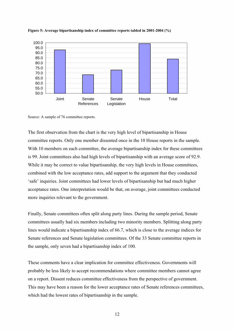
Figure 5: Average bipartisanship index of committee reports tabled in 2001-2004 (%)
50.055.060.065.070.075.080.085.090.095.0
100.0
Joint SenateReferences
SenateLegislation
House Total
Source: A sample of 76 committee reports.
The first observation from the chart is the very high level of bipartisanship in House
committee reports. Only one member dissented once in the 10 House reports in the sample.
With 10 members on each committee, the average bipartisanship index for these committees
is 99. Joint committees also had high levels of bipartisanship with an average score of 92.9.
While it may be correct to value bipartisanship, the very high levels in House committees,
combined with the low acceptance rates, add support to the argument that they conducted
‘safe’ inquiries. Joint committees had lower levels of bipartisanship but had much higher
acceptance rates. One interpretation would be that, on average, joint committees conducted
more inquiries relevant to the government.
Finally, Senate committees often split along party lines. During the sample period, Senate
committees usually had six members including two minority members. Splitting along party
lines would indicate a bipartisanship index of 66.7, which is close to the average indices for
Senate references and Senate legislation committees. Of the 33 Senate committee reports in
the sample, only seven had a bipartisanship index of 100.
These comments have a clear implication for committee effectiveness. Governments will
probably be less likely to accept recommendations where committee members cannot agree
on a report. Dissent reduces committee effectiveness from the perspective of government.
This may have been a reason for the lower acceptance rates of Senate references committees,
which had the lowest rates of bipartisanship in the sample.
13
Media coverage
Committees work in a political environment. Therefore, one way of comparing reports is
whether they receive media coverage or not. To measure this coverage, an index was prepared
based on the parliamentary library’s databases. The library maintains comprehensive coverage
of five newspapers: the Sydney Morning Herald, the Age, the Australian, the Australian
Financial Review and the Canberra Times.18 These papers were searched electronically for
any mention of the reports in the sample for two days after tabling. Focussing on the period
shortly after tabling was more manageable than developing a profile across the life of an
inquiry, which could last over a year. Two days were chosen because some Senate reports
were tabled later in the day and missed the deadline for publication in the next day’s paper.
The index had two components. The first was whether a report was mentioned in a particular
paper. For each paper, the report received one point. The second component involved how
close to the front page the article was located in each paper, and therefore how newsworthy it
was. The inverse of the page number was calculated for this, so if an article was on page one
the report received one extra point. Page two resulted in half a point, page three one third of a
point and so on. Each paper had a potential score of two per committee report, and combining
the result of the five papers gave a potential score between zero and 10. Zero equated to no
mention in any of the five papers and 10 equated to being on page one in all of the papers.
Figure six has the results for each committee type.
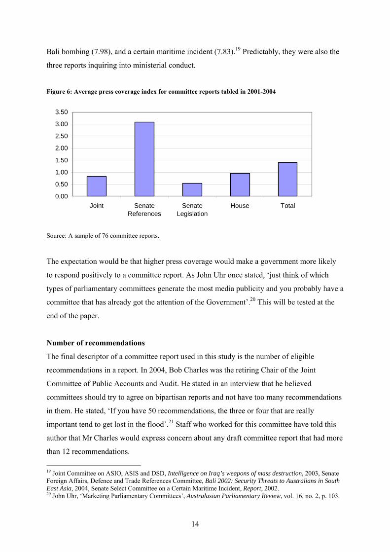
There are two main observations from the graph. Firstly, committee reports overall do not
receive a great deal of media. The average index for the whole sample is 1.39, which roughly
equates to an article on page three in one of the five sampled newspapers. The second
observation is that Senate references committees received the most coverage by a clear
margin. Their score was 3.09, which equates to mentions in three of the five papers at the end
of the news section. Eight reports in the sample received media scores greater than five, and
all but one related to inquiries by Senate references committees. The three highest scoring
reports in the sample covered the intelligence on Iraq’s weapons of mass destruction (10), the
18 It would have been preferable to use the newspapers with the highest circulations, but the library does not keep comprehensive records of them. These papers are the Herald Sun, the Daily Telegraph, the Courier Mail and the West Australian. The Sydney Morning Herald comes fifth.
14
Bali bombing (7.98), and a certain maritime incident (7.83).19 Predictably, they were also the
three reports inquiring into ministerial conduct.
Figure 6: Average press coverage index for committee reports tabled in 2001-2004
0.00
0.50
1.00
1.50
2.00
2.50
3.00
3.50
Joint SenateReferences
SenateLegislation
House Total
Source: A sample of 76 committee reports.
The expectation would be that higher press coverage would make a government more likely
to respond positively to a committee report. As John Uhr once stated, ‘just think of which
types of parliamentary committees generate the most media publicity and you probably have a
committee that has already got the attention of the Government’.20 This will be tested at the
end of the paper.
Number of recommendations
The final descriptor of a committee report used in this study is the number of eligible
recommendations in a report. In 2004, Bob Charles was the retiring Chair of the Joint
Committee of Public Accounts and Audit. He stated in an interview that he believed
committees should try to agree on bipartisan reports and not have too many recommendations
in them. He stated, ‘If you have 50 recommendations, the three or four that are really
important tend to get lost in the flood’.21 Staff who worked for this committee have told this
author that Mr Charles would express concern about any draft committee report that had more
than 12 recommendations.
19 Joint Committee on ASIO, ASIS and DSD, Intelligence on Iraq’s weapons of mass destruction, 2003, Senate Foreign Affairs, Defence and Trade References Committee, Bali 2002: Security Threats to Australians in South East Asia, 2004, Senate Select Committee on a Certain Maritime Incident, Report, 2002. 20 John Uhr, ‘Marketing Parliamentary Committees’, Australasian Parliamentary Review, vol. 16, no. 2, p. 103.
15
In the sample, the number of eligible recommendations in reports ranged from one to 89.
Three reports had 50 or more recommendations and they were all by Senate references
committees. The average number of recommendations was 11. Although this paper makes the
simplifying assumption that all recommendations in reports are equally important, Mr
Charles’ economical philosophy can be tested. The statistical study that follows checks
whether the number of recommendations affects the likelihood of the government accepting at
least one recommendation in a report (whether the committee is effective) and if it affects the
overall acceptance rate (how a committee can be more effective).
Modelling government responses22 Minimum effectiveness
This part of the study involved running a regression of a number of characteristics of
committee reports (for example, type of committee) against whether the government accepted
at least one recommendation in a report.23 The aim was to extract the effect of each individual
characteristic to create an equation that generated the probability that the government would
accept at least one recommendation in a report. For example, while Senate reference
committees tended to have low rates of bipartisanship, the model can provide an estimate, on
average, of what would happen to the probability of effectiveness if one of those committees
increased its bipartisanship measure but left everything else the same. The model also checks
whether any characteristics are not statistically significant. That is, their effect in the sample
may vary so much that it is not possible to reliably predict what their effect is. If any
characteristic varied this much, it was removed from the model. After removing
characteristics with low reliability, a model with seven characteristics was created. The results
are in table two. A more thorough discussion of these processes is in the appendix.
21 ‘Straight Shooter’, About the House, March 2004, p. 26. 22 The EasyReg package was used for the regressions. See Bierens, H. J. (2007), ‘EasyReg International’, Department of Economics, Pennsylvania State University, University Park, PA 16802, USA (http://econ.la.psu.edu/~hbierens/EASYREG.HTM). 23 A logit model. An acceptance rate of zero equated to a negative result and an acceptance rate greater than zero equated to a positive result.
16
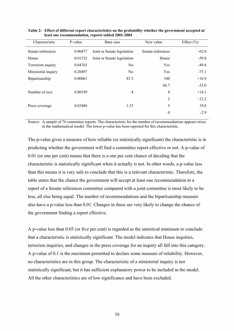
Table 2: Effect of different report characteristics on the probability whether the government accepted at least one recommendation, reports tabled 2001-2004
Characteristic P-value Base case New value Effect (%)
Senate references 0.00477 Joint or Senate legislation Senate references -62.0
House 0.01532 Joint or Senate legislation House -59.0
Terrorism inquiry 0.04763 No Yes -49.4
Ministerial inquiry 0.20497 No Yes -75.1
Bipartisanship 0.00061 83.3 100 +16.9
66.7 -33.0
Number of recs 0.00199 4 8 +14.1
2 -12.2
Press coverage 0.03480 1.33 5 19.8
0 -2.9
Source: A sample of 76 committee reports. The characteristic for the number of recommendations appears twice in the mathematical model. The lower p-value has been reported for this characteristic.
The p-value gives a measure of how reliable (or statistically significant) the characteristic is in
predicting whether the government will find a committee report effective or not. A p-value of
0.01 (or one per cent) means that there is a one per cent chance of deciding that the
characteristic is statistically significant when it actually is not. In other words, a p-value less
than this means it is very safe to conclude that this is a relevant characteristic. Therefore, the
table states that the chance the government will accept at least one recommendation in a
report of a Senate references committee compared with a joint committee is most likely to be
less, all else being equal. The number of recommendations and the bipartisanship measure
also have a p-value less than 0.01. Changes in these are very likely to change the chance of
the government finding a report effective.
A p-value less than 0.05 (or five per cent) is regarded as the statistical minimum to conclude
that a characteristic is statistically significant. The model indicates that House inquiries,
terrorism inquiries, and changes in the press coverage for an inquiry all fall into this category.
A p-value of 0.1 is the maximum permitted to declare some measure of reliability. However,
no characteristics are in this group. The characteristic of a ministerial inquiry is not
statistically significant, but it has sufficient explanatory power to be included in the model.
All the other characteristics are of low significance and have been excluded.

17
Tested against the 76 reports in the sample, the model predicts the correct result 81.6 per cent
of the time. This compares against 50 per cent for flipping a coin or 63.2 per cent for
automatically predicting a positive result in all cases. Therefore, the model has reasonable
predicting power.
The table adopts a hypothetical base case of a joint committee tabling a report with four
recommendations on a topic other than terrorism. The bipartisanship score is 83.3 per cent,
equivalent to 10 members out of 12 agreeing on the report. This is close to the sample average
of 83.9 per cent. With these characteristics, the model predicts a 76.3 per cent chance that the
government would accept at least one recommendation in the report. If, however, a report
with these characteristics was tabled by a Senate references committee, then the chance for
effectiveness would drop by 62 per cent to 14.3 per cent.24 This does not mean that exactly
the same report would have a reduced chance simply because a different type of committee
wrote it, although this type of effect may be involved. What it most likely means is that the
different approaches taken by a Senate references committee in terms of topic and tone
reduces the chance that the government will be prepared to accept some of its
recommendations, compared with a joint committee.
Another comment to make from the table is that the largest movements in the chance of
effectiveness tend to be due to the type of committee running an inquiry, rather than the
characteristics of the report itself. A change in the type of committee for this base case leads
to changes in the order of 60 per cent. For the other statistically significant characteristics, the
largest changes occur with bipartisanship and terrorism inquiries. Both of these effects are in
the order of 50 per cent.
These results confirm some of the observations made earlier in the paper. The exception is
Bob Charles’ comment about limiting the number of recommendations. What appears to be
happening instead is that having more recommendations in a report increases the chances that
there will be something that the government finds useful in it. This is similar to a lottery
effect. The more tickets one buys in a lottery, the greater the chance of winning a prize. The
24 The two models in the paper are non-linear. Therefore, the 62 per cent reduction only applies to the specific circumstances in the base case. Variations in the base case will lead to changes in the effect of a Senate references inquiry and for all other characteristics as well.
18
impact of this characteristic is a result of setting a non-zero acceptance rate as the benchmark,
rather than a particular proportion, such as 50 per cent.
The importance of the number of recommendations particularly affects the performance of
Senate legislation committees. These committees tended to have a low number of majority
recommendations. The majority comprised government members and they generally only
made a small number of recommendations – the average was two. This was because the bills
were referred by opposition parties in the Senate and it appears that government Senators
were only interested in suggesting changes to legislation if they saw a strong case for doing
so. Therefore, the explanation for the similarity between joint committees and Senate
legislation committees in the model and the difference in their acceptance rates is because the
majority on Senate legislation committees tended to make few recommendations.
The criticism of this model is that committees can inflate their effectiveness by tabling long
reports with a large number of recommendations. There are a number of responses to this
concern. Firstly, it is not the only measure of effectiveness under the framework. For instance,
the acceptance rate can be considered to be a supplementary performance indicator to this
initial measure of effectiveness. The views of the legislature, stakeholders and the public must
also be considered in assessing overall effectiveness. Inflating one effectiveness measure is
likely to adversely affect the perspectives of the other three groups. Further, it is advisable to
compare any effectiveness measure with an efficiency measure as well. For instance, it should
be possible to publish the cost of a committee report, which Canadian committees have done
in the past and the Audit Office of New South Wales does for its performance audits.25
Including the cost of an inquiry in the report should moderate any such behaviour.
Increasing the acceptance rate
The next step in the analysis was to run a regression of what factors would increase the
acceptance rate, assuming the government accepts at least one recommendation in the
25 Brian O’Neal, ‘Senate Committees: Role and Effectiveness’, Canadian Parliamentary Information and Research Service, June 1994, http://www.parl.gc.ca/information/library/PRBpubs/bp361-e.htm, (accessed 17 October 2007. New South Wales performance audit reports available at http://www.audit.nsw.gov.au/publications/reports/performance/performance_reports.htm (accessed 21 December 2007).

19
report.26 In this case, a sub sample of the 48 effective committee reports was used. The
research question was to determine which characteristics made an effective report more so
from the perspective of the government. The results for the ‘predicted acceptance rate’ are in
table three.
Table 3: Effect of different report characteristics on government acceptance rate, assuming at least one
recommendation is accepted, reports tabled 2001-2004
Characteristic P-value Base case New value Effect (%)
Senate References 0.00019 Joint or Senate legislation Senate references -49.8
House 0.00024 Joint or Senate legislation House -22.9
Administration inquiry 0.00000 Policy inquiry Administration +22.4
Bills inquiry 0.01457 Policy inquiry Bill +29.1
Press coverage 0.00383 1.33 5.0 +21.5
0 -10.6
Number of recs (House) 0.00024 4 8 -3.2
2 +0.8
Number of recs (Admin) 0.00003 4 8 -33.7
2 11.3
Source: A sub-sample of 48 committee reports. The characteristics for House inquiries, administrative inquiries and the number of recommendations each appear more than once in the mathematical model. The lowest p-values have been reported for these characteristics.
There are a number of similarities in these results with those in table two. The effects of
Senate references committees, House committees and press coverage are all statistically
significant and the same sign as before. The differences are the new characteristics of an
administration inquiry and bills inquiry, both of which increase the acceptance rate. The
categories of terrorism and ministerial inquiry do not have sufficient explanatory power to be
included in the model. Overall, the model performs reasonably well. It explains 63.1 per cent
of the variation in the regression, which is similar to stating that it explains 63.1 per cent of
the variation in the positive acceptance rates.27
An interesting change from table two is that, while the number of recommendations is still
statistically significant, it has changed sign. In other words, while a larger report is more
likely to achieve a minimum level of effectiveness, it is also more likely to have a lower
26 An ordinary least squares regression on the natural log of the ratio between the acceptance rate and 100 minus the acceptance rate. Algebraically, this is ln(AR/(100-AR)). Where the acceptance rate was 100, it was transformed to 99 for the purposes of this calculation.
20
acceptance rate. This may reflect the law of diminishing marginal returns. When deliberating
on a report, a committee is likely to make the most important and best recommendations its
priority. Less important recommendations become subsequent additions ‘on the margin’. A
larger report will have, on average, more marginal recommendations, which will reduce the
likely acceptance rate. However, this effect only applied to House and administrative
inquiries, which comprised 30.3 per cent of the sample (23 reports).28
Similar to before, the effect of each characteristic is demonstrated against a hypothetical case
of a joint committee report with four recommendations, a bipartisanship index of 83.3, and a
press coverage index of 1.33. The exception is the entries for the number of
recommendations. Because the effect of the number of recommendations is limited to House
and administrative inquiries, the values in the effect column in the last four rows are based on
assuming a House and administrative (joint) committee respectively.
The type of committee conducting the inquiry again has a large effect. Changing from a joint
committee to either a Senate references or House committee reduces the acceptance rate by up
to 50 per cent. However, a Senate legislation committee is not statistically different to a joint
committee. Another large-scale effect is if the committee in question examined a bill. Where
the government decided to accept some of the recommendations for a bill inquiry, this
increased the acceptance rate by almost 30 per cent. In other words, the government tended to
respond to bill inquiries on an ‘all or nothing’ basis. The government also responded to press
coverage when it decided to accept some recommendations in a report. A large increase in
press coverage to five on the index (equivalent to page four in four of the five surveyed
papers) increased the acceptance rate by over 20 per cent.
These results confirm some of the initial discussion and are probably more in line with
expectations than the results for the first model. For instance, it provides some support for
Bob Charles’ views that adding more recommendations to a report will not necessarily make
it more effective, at least in relation to House and administrative inquiries. It is also in line
with Derek Hawes’ observation that governments are more likely to be receptive to reports on
administrative issues, rather than policy reports.
27 The independent variable is the log of the acceptance ratio, not the acceptance rate.

21
The sub-sample of 48 reports is different to the full sample of 76. For example, the sub-
sample has a smaller proportion of reports that involved high levels of political dispute. This
is demonstrated by differing bipartisanship rates. In the sub sample, the average is 90.5 and in
the rest of the sample (the remaining 28 reports) it is 72.6. To a large extent, the reports
excluded from the sub-sample comprise those highly controversial reports that the
government did not respond to because their political opponents took the opportunity to take a
combative approach, rather than a cooperative one.
Applications While this analysis assists in explaining the government’s responses to reports tabled between
the 2001 and 2004 elections, committee members can also use it to assist in their decision
making about reports. In order for these applications to be valid, they must meet a number of
assumptions. For example, the analysis assumes that all recommendations in a report are
equally important. In the real world, this is rarely the case. Further, there has been a change of
government since the sample period. Although there are similarities between governments,
there are also differences. To apply the results of the regression to future governments implies
that the differences between governments in relation to committee reports are negligible. We
also know that the models leave a large proportion of the government response unexplained.
Therefore, using the regression results in this way might best be regarded as indicative of the
tradeoffs that committees now face, rather than authoritative.
Maintaining bipartisanship
Let us assume a joint committee is deliberating on a report with nine recommendations on a
non-terrorism policy matter. The expected press coverage is 1.33 and all 20 committee
members are expected to agree on the report. Let us also assume that, due to external factors,
the opposition members then inform the committee that there is a number of
recommendations that they cannot support. How should the government members approach
the negotiations?
If we assume that the government members wish to maximise the chance that at least some
recommendations will be implemented, then they should try to secure full bipartisanship. For
example, if the opposition members only support five recommendations and the government
28 No House committee conducted an administrative inquiry in the sample.

22
members agree to this reduction in the report, then the chance of the government accepting at
least one recommendation is 94.8 per cent. If the committee adopts nine recommendations
and the eight opposition members dissent, then the chance of the government accepting at
least one recommendation drops to 71.9 per cent. This calculation assumes that there is a
small increase in press coverage due to the dispute (to 2.67).
The other scenario is that the 12 government members are not risk averse and they instead
wish to maximise the number of recommendations that the government will probably accept.
This figure is calculated by multiplying the number of recommendations by the probability
the government will accept at least one recommendation (first model) by the predicted
acceptance rate (second model). If the committee adopts nine recommendations with eight
opposition members dissenting, the likely number of recommendations that the government
will accept is 4.78. What will be the effect of government members trading off some
recommendations to secure full bipartisanship? While 100 per cent bipartisanship will
maximise the likely acceptance rate, trading off recommendations will reduce the number of
recommendations available for the government’s consideration. If we assume that the
government members only need to drop one recommendation to secure the agreement of the
opposition members, then the likely number of accepted recommendations will be 5.03. In
this case, negotiating to secure bipartisanship is worthwhile.
If the opposition members require two recommendations to be dropped from the report to
achieve consensus, leaving seven recommendations in the report, then the likely number that
the government will accept is 4.37. Therefore, the government members know that dropping
one recommendation to secure consensus will make them better off, but it is not worth trading
off any more. If the opposition members require more than this, then the government
members should keep all nine recommendations and accept the consequences of a minority
report. Of course, opposition members can make these calculations as well.
This case study suggests that a majority’s approach to bipartisanship will depend on how risk
averse it is. The more risk averse a committee majority, the more likely it is to seek
consensus. However, bipartisanship is still relevant to committee majorities that are less risk
averse. Where committees are seeking to maximise the likely number of accepted
recommendations, then negotiating to achieve an agreed report is worthwhile, provided the

23
majority does not give up too many recommendations. Bipartisanship has value in this case,
but it is possible to pay too high a price to secure it.
Choice of committee
Tables two and three show there is a clear difference between the effects of an inquiry being
conducted by either a joint or Senate legislation committee on the one hand, and a Senate
references or House committee on the other. For example, the chance that the government
would accept at least one recommendation drops by over 50 per cent. Assume that a
parliamentarian wanted a committee to investigate a policy issue and they wanted the
government to commit to new action on it. Let us further assume that they did not mind which
type of committee conducted the inquiry. These figures suggest that the Senator or Member in
question should lobby to have the inquiry conducted by a joint committee, rather than a
Senate references or House committee.
Some areas of government activity are specifically covered by joint committees with
reasonably wide terms of reference. These include foreign affairs, defence, trade, financial
services, security, crime and migration. For activities outside these areas there is the option of
lobbying to have the inquiry conducted by the Joint Committee on Public Accounts and
Audit. This committee has wide terms of reference, including the receipt and expenditure of
funds by the Commonwealth and any circumstances connected with them.29 It can inquire into
almost any area of Commonwealth activity. During its history, it has almost always delivered
bipartisan reports, which increases the chances of the government accepting its
recommendations. Therefore, there is theoretically a joint committee available for every type
of inquiry.
More or less recommendations?
The final topic in this area concerns whether the size of the report has a large impact on the
acceptance rate. After combining the two models, figure seven shows the effect of increasing
the number of recommendations in a report on the expected acceptance rate. The base case in
this example assumes a joint committee policy inquiry with 90 per cent bipartisanship and no
press coverage.
29 See sub-section 8(1) of the Public Accounts and Audit Committee Act 1951.

24
Figure 7: Impact of recommendations on committee effectiveness, reports tabled in 2001-2004
0
10
20
30
40
50
60
70
80
1 3 5 7 9 11 13 15 17 19 21 23
Number of recommendations
Expe
cted
acc
epta
nce
rate
(%)
Joint & Senate Leg'nHouseAdministrative (Joint)Senate References
Source: A sample of 76 committee reports. The line for administrative inquiries stops short to be consistent with
the low number of recommendations for these inquiries in the sub-sample of 48. Projections beyond the sample range are not valid.
In terms of maximising the expected acceptance rate, the optimal number of recommendations
depends on the committee and the inquiry. For House committees, the maximum expected
acceptance rate occurs at 13 recommendations. For joint committees conducting
administrative inquiries, it occurs at three recommendations. There is no particular maximum
point for joint committees, Senate legislation committees or Senate references committees.
However, the value of added recommendations tapers off for joint and Senate legislation
committees after 10 recommendations. This result supports the views of Bob Charles. In
terms of the proportion of recommendations accepted, large reports tend to be inefficient.
Limiting reports to a dozen recommendations in most cases appears to be a good compromise
between properly covering a topic and being efficient. The exceptions are administrative
inquiries and Senate references inquiries. For the former, a limit of five or six
recommendations is probably a good benchmark. For Senate references inquiries, there does
not appear to be any suitable report size. However, it should be noted that these inquiries were
often a platform for opposition parties to engage in political debate with the government. The
government response may not have been relevant to their effectiveness.
25
Conclusion In the sample of 76 reports, the government accepted at least one recommendation in 48
cases. In other words, where a committee report suggested new action to the government, the
government found these suggestions useful 63.2 per cent of the time. While different
observers may have different views about appropriate benchmarks, it seems fair to judge this
a reasonable level of performance.
From the perspective of governments, the most effective committees, on average, are joint
committees. The average acceptance rate for joint committee reports during the sample period
was over 50 per cent, which exceeded the average acceptance rate for all other committee
types by at least 20 per cent. Two regressions were used to extract the individual effects of
report characteristics. The first stage focussed on what makes a committee report effective,
and the second on what makes effective reports more so. The regressions found a clear
difference between joint committee reports compared with Senate references and House
committee reports. Interestingly, the size of the effect was similar for Senate references and
House committees in both regressions. This suggests that they are fundamentally similar types
of committees, despite the former being the only committees where the opposition had a
majority. Perhaps the main reason is that they are both single-chamber committees with non-
specific roles. From the government’s perspective, House committees tended to be more
effective due to their higher levels of bipartisanship.
Senate legislation committees were the ‘dark horses’ of the study. In terms of acceptance
rates, they do not appear to perform particularly well. However, once the various report
characteristics are taken into account, including bill reports, they are statistically no different
to joint committees. This suggests that there is something inherently valuable to government
about their work. It also corroborates John Uhr’s comments that, on average, committees are
better at refining government proposals, rather than conducting larger scale policy work.30
Aside from the type of committee, the most important factors were the number of
recommendations, bipartisanship, press coverage, and the inquiry topic. With these results,
the study reinforces some prior observations of committees. Gavin Drewry stated that
committees are at their most effective when they conduct contentious inquiries but deliver
26
bipartisan reports. Bob Charles set a limit of a dozen recommendations per report. From the
perspective of government, these are a prescription for committee effectiveness.
30 John Uhr, Parliamentary Committees: What Are Appropriate Performance Standards? Discussion Paper prepared for Constitutional Centenary Foundation, 1993, p. 16.

27
Statistical appendix
Summary data The text provides a detailed examination of the summary data. For completeness, summary
data tables for the two regressions are below. The independent variable for each regression is
listed on the first row of each table.
Table 4: Summary data for the logit model of minimum committee effectiveness
Variable Minimum Maximum Average Standard Error
Effectiveness dummy 0 1 0.63 0.49
Senate references dummy 0 1 0.26 0.44
Senate legislation dummy 0 1 0.17 0.38
House dummy 0 1 0.13 0.34
Terrorism dummy 0 1 0.13 0.34
Immigration dummy 0 1 0.07 0.25
Administration dummy 0 1 0.17 0.38
Bills dummy 0 1 0.26 0.44
Ministerial dummy 0 1 0.04 0.20
Legislated functions dummy 0 1 0.28 0.45
Number of recommendations 1 89 10.84 14.38
Bipartisanship index 25 100 83.92 20.59
Press coverage index 0 10 1.39 2.31
Source: A sample of 76 committee reports.
One observation from table four is that there are only three inquiries into ministerial conduct
in the sample. This means that this dummy variable has reduced chances of being found to be
statistically significant. Another observation is that the three continuous variables on the last
rows are skewed. For example, the mean number of recommendations is 11, but the
maximum is 89. A linear specification implies that a change from 1 recommendation to 11
will be the same as that from 40 to 50. Practically, however, any report having over 20
recommendations would be considered a large report. In theory, the impact of changing the
number of recommendations from 1 to 11 would be much greater than a change from 40 to
50. This suggests that the squared term of this variable could be added to the model to adjust
for non-linear effects. A similar argument could be made for the other continuous variables.
28
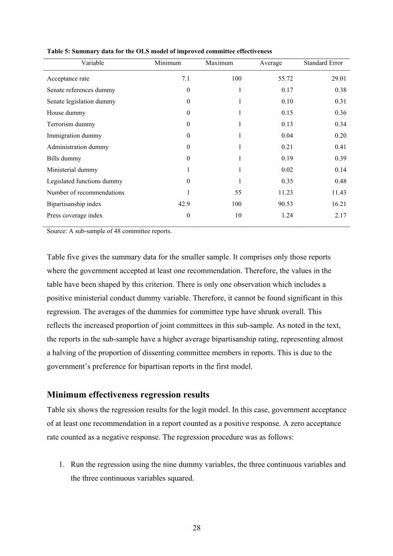
Table 5: Summary data for the OLS model of improved committee effectiveness
Variable Minimum Maximum Average Standard Error
Acceptance rate 7.1 100 55.72 29.01
Senate references dummy 0 1 0.17 0.38
Senate legislation dummy 0 1 0.10 0.31
House dummy 0 1 0.15 0.36
Terrorism dummy 0 1 0.13 0.34
Immigration dummy 0 1 0.04 0.20
Administration dummy 0 1 0.21 0.41
Bills dummy 0 1 0.19 0.39
Ministerial dummy 1 1 0.02 0.14
Legislated functions dummy 0 1 0.35 0.48
Number of recommendations 1 55 11.23 11.43
Bipartisanship index 42.9 100 90.53 16.21
Press coverage index 0 10 1.24 2.17
Source: A sub-sample of 48 committee reports.
Table five gives the summary data for the smaller sample. It comprises only those reports
where the government accepted at least one recommendation. Therefore, the values in the
table have been shaped by this criterion. There is only one observation which includes a
positive ministerial conduct dummy variable. Therefore, it cannot be found significant in this
regression. The averages of the dummies for committee type have shrunk overall. This
reflects the increased proportion of joint committees in this sub-sample. As noted in the text,
the reports in the sub-sample have a higher average bipartisanship rating, representing almost
a halving of the proportion of dissenting committee members in reports. This is due to the
government’s preference for bipartisan reports in the first model.
Minimum effectiveness regression results Table six shows the regression results for the logit model. In this case, government acceptance
of at least one recommendation in a report counted as a positive response. A zero acceptance
rate counted as a negative response. The regression procedure was as follows:
1. Run the regression using the nine dummy variables, the three continuous variables and
the three continuous variables squared.

29
2. Note which variables had a t-value less than one. Drop these from the regression and
run it again, culling variables each time that have a t-value less than one. The result
from this process is model A.
3. Run an artificial regression for heteroskedasticity on the error terms and include cross
products and squares as independent variables. Note which ones are statistically
significant.
4. Add these candidates to model A and repeat the regression, dropping variables with a
t-value less than one. The result is model B.
5. Compare models A and B for goodness of fit and select the preferred model.
The following cross products showed a relationship with the error term and were added to
model A: house x press2, recommendations x bipartisanship, recommendations3,
bipartisanship x press2, bipartisanship x recommendations2, and recommendations4.
Table 6: Regression results for the logit model of minimum committee effectiveness
Variable Model A Model B
Coefficient t-value Coefficient t-value
Senate references dummy -2.963 -2.82 *** -2.539 -2.34 **
House dummy -2.739 -2.42 ** -3.373 -2.30 **
Terrorism dummy -2.173 -1.98 ** -1.207 -1.22
Ministerial dummy -5.612 -1.27
Recommendations 0.323 3.09 *** -1.156 -2.50 **
Recommendations2 -0.00453 -2.45 ** 0.0496 2.33 **
Bipartisanship 0.0868 3.43 ***
Press2 0.0876 2.11 **
Recommendations x Bipartisanship 0.0213 2.95 ***
Recommendations2 x Bipartisanship -0.000798 -2.46 **
Intercept -7.434 -3.28 *** -0.729 -1.36
Loglikelihood -28.967 -30.396
Akaike Information Criterion 0.999 1.010
Schwarz Information Criterion 1.275 1.256
Source: A sample of 76 committee reports. * indicates significant at the 10 per cent level of significance, ** indicates significant at the five per cent level of significance and *** indicates significant at the one per cent level of significance.
In examining table six, the first task is to select the preferred model. Model A has better
scores for the loglikelihood and the Akaike Information Criterion. Model B has a better score
30
for the Schwarz Information Criterion, which places a greater penalty on adding extra
variables to the model. Model A also has the advantage of being simpler to interpret and was
the first model generated in the process. Although the differences are not great, model A was
selected because the advantages offered by model B are less than in model A.
There are two main additional comments to those made in the text about the effect of the
variables. The first is that it is possible to calculate the number of recommendations that
would maximise the chances of the government accepting at least one recommendation in a
report. This is because the coefficient for recommendations2 has a negative sign, which means
the second derivative will as well. Differentiating the regression equation by
recommendations and solving gives a global maximum of 36 recommendations. In other
words, there is a limit to the lottery effect discussed in the text. If the government did not find
anything worth accepting in a report with 36 recommendations, then adding more
recommendations would not, on average, improve the report’s chances of being deemed
effective by the government.
The second comment is that press coverage appears as a squared term. The effect of this is to
give greater weight to higher amounts of media coverage. For example, an increase in press
from zero to five would increase the log of the probability ratio by 2.19, but an increase from
five to 10 would increase it by an extra 6.57, or three times again. The interpretation of this is
that it was possible to use the media to push the government into accepting some
recommendations in a report, but the media coverage had to be intense, such as being on the
front page of as many newspapers as possible. Interestingly, the press coverage index
included a bonus for front page coverage and the model took this further by adopting the
index’s squared term.
In logit models, the diagnostic issues are specification and heteroskedasticity. Davidson and
MacKinnon’s ordinary least squares (OLS) artificial regression was used to conduct these
diagnostic tests.31 The specification test was:
Vt-1/2(yt – Ft) = Vt
-1/2ftXtb + aVt-1/2(Xtβ)2ft + residual
31
Vt = the variance of the error term = Pt – Pt2
Pt = the predicted probability = Ft
yt = the observed dependent variable
ft = the derivative of Ft = Vt (logit model only)
Xtβ = ln(Pt/(1-Pt))
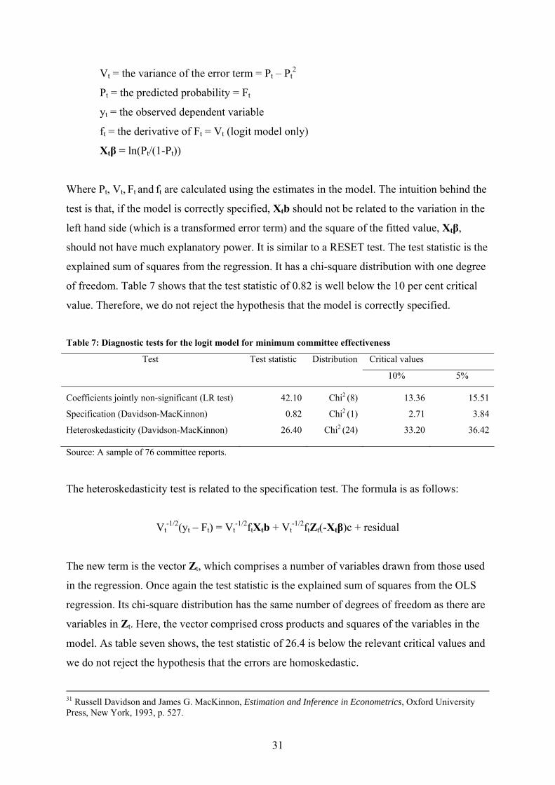
Where Pt, Vt, Ft and ft are calculated using the estimates in the model. The intuition behind the
test is that, if the model is correctly specified, Xtb should not be related to the variation in the
left hand side (which is a transformed error term) and the square of the fitted value, Xtβ,
should not have much explanatory power. It is similar to a RESET test. The test statistic is the
explained sum of squares from the regression. It has a chi-square distribution with one degree
of freedom. Table 7 shows that the test statistic of 0.82 is well below the 10 per cent critical
value. Therefore, we do not reject the hypothesis that the model is correctly specified.
Table 7: Diagnostic tests for the logit model for minimum committee effectiveness
Test Test statistic Distribution Critical values
10% 5%
Coefficients jointly non-significant (LR test) 42.10 Chi2 (8) 13.36 15.51
Specification (Davidson-MacKinnon) 0.82 Chi2 (1) 2.71 3.84
Heteroskedasticity (Davidson-MacKinnon) 26.40 Chi2 (24) 33.20 36.42
Source: A sample of 76 committee reports.
The heteroskedasticity test is related to the specification test. The formula is as follows:
Vt-1/2(yt – Ft) = Vt
-1/2ftXtb + Vt-1/2ftZt(-Xtβ)c + residual
The new term is the vector Zt, which comprises a number of variables drawn from those used
in the regression. Once again the test statistic is the explained sum of squares from the OLS
regression. Its chi-square distribution has the same number of degrees of freedom as there are
variables in Zt. Here, the vector comprised cross products and squares of the variables in the
model. As table seven shows, the test statistic of 26.4 is below the relevant critical values and
we do not reject the hypothesis that the errors are homoskedastic.
31 Russell Davidson and James G. MacKinnon, Estimation and Inference in Econometrics, Oxford University Press, New York, 1993, p. 527.
32
There are a number of ways of assessing the explanatory power of the model. The first is to
test the hypothesis that the slope coefficients are jointly equal to zero. Table seven shows the
results for the likelihood ratio test, which was calculated against the null likelihood of -50.02.
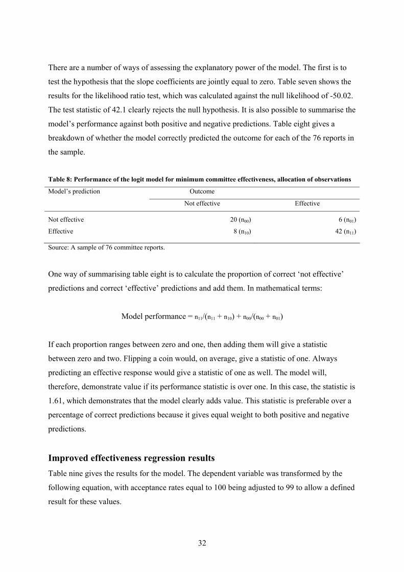
The test statistic of 42.1 clearly rejects the null hypothesis. It is also possible to summarise the
model’s performance against both positive and negative predictions. Table eight gives a
breakdown of whether the model correctly predicted the outcome for each of the 76 reports in
the sample.
Table 8: Performance of the logit model for minimum committee effectiveness, allocation of observations
Model’s prediction Outcome
Not effective Effective
Not effective 20 (n00) 6 (n01)
Effective 8 (n10) 42 (n11)
Source: A sample of 76 committee reports.
One way of summarising table eight is to calculate the proportion of correct ‘not effective’
predictions and correct ‘effective’ predictions and add them. In mathematical terms:
Model performance = n11/(n11 + n10) + n00/(n00 + n01)
If each proportion ranges between zero and one, then adding them will give a statistic
between zero and two. Flipping a coin would, on average, give a statistic of one. Always
predicting an effective response would give a statistic of one as well. The model will,
therefore, demonstrate value if its performance statistic is over one. In this case, the statistic is
1.61, which demonstrates that the model clearly adds value. This statistic is preferable over a
percentage of correct predictions because it gives equal weight to both positive and negative
predictions.
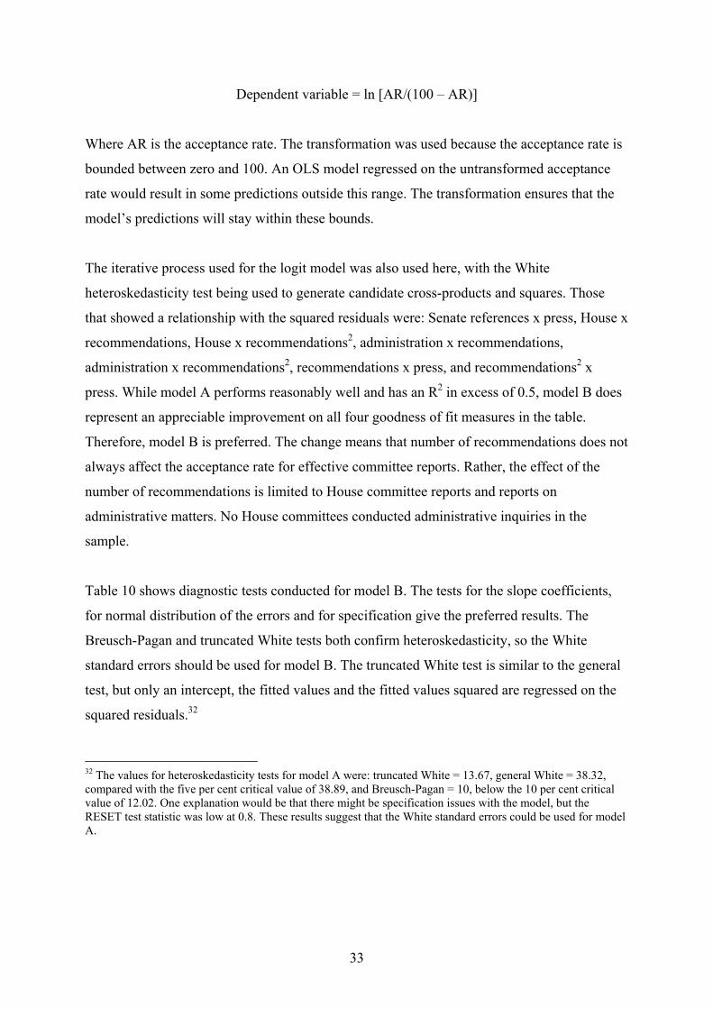
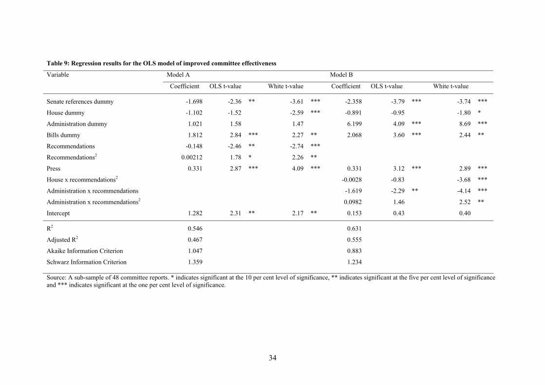
Improved effectiveness regression results Table nine gives the results for the model. The dependent variable was transformed by the
following equation, with acceptance rates equal to 100 being adjusted to 99 to allow a defined
result for these values.
33
Dependent variable = ln [AR/(100 – AR)]
Where AR is the acceptance rate. The transformation was used because the acceptance rate is
bounded between zero and 100. An OLS model regressed on the untransformed acceptance
rate would result in some predictions outside this range. The transformation ensures that the
model’s predictions will stay within these bounds.
The iterative process used for the logit model was also used here, with the White
heteroskedasticity test being used to generate candidate cross-products and squares. Those
that showed a relationship with the squared residuals were: Senate references x press, House x
recommendations, House x recommendations2, administration x recommendations,
administration x recommendations2, recommendations x press, and recommendations2 x
press. While model A performs reasonably well and has an R2 in excess of 0.5, model B does
represent an appreciable improvement on all four goodness of fit measures in the table.
Therefore, model B is preferred. The change means that number of recommendations does not
always affect the acceptance rate for effective committee reports. Rather, the effect of the
number of recommendations is limited to House committee reports and reports on
administrative matters. No House committees conducted administrative inquiries in the
sample.
Table 10 shows diagnostic tests conducted for model B. The tests for the slope coefficients,
for normal distribution of the errors and for specification give the preferred results. The
Breusch-Pagan and truncated White tests both confirm heteroskedasticity, so the White
standard errors should be used for model B. The truncated White test is similar to the general
test, but only an intercept, the fitted values and the fitted values squared are regressed on the
squared residuals.32
32 The values for heteroskedasticity tests for model A were: truncated White = 13.67, general White = 38.32, compared with the five per cent critical value of 38.89, and Breusch-Pagan = 10, below the 10 per cent critical value of 12.02. One explanation would be that there might be specification issues with the model, but the RESET test statistic was low at 0.8. These results suggest that the White standard errors could be used for model A.
34
Table 9: Regression results for the OLS model of improved committee effectiveness
Variable Model A Model B
Coefficient OLS t-value White t-value Coefficient OLS t-value White t-value
Senate references dummy -1.698 -2.36 ** -3.61 *** -2.358 -3.79 *** -3.74 ***
House dummy -1.102 -1.52 -2.59 *** -0.891 -0.95 -1.80 *
Administration dummy 1.021 1.58 1.47 6.199 4.09 *** 8.69 ***
Bills dummy 1.812 2.84 *** 2.27 ** 2.068 3.60 *** 2.44 **
Recommendations -0.148 -2.46 ** -2.74 ***
Recommendations2 0.00212 1.78 * 2.26 **
Press 0.331 2.87 *** 4.09 *** 0.331 3.12 *** 2.89 ***
House x recommendations2 -0.0028 -0.83 -3.68 ***
Administration x recommendations -1.619 -2.29 ** -4.14 ***
Administration x recommendations2 0.0982 1.46 2.52 **
Intercept 1.282 2.31 ** 2.17 ** 0.153 0.43 0.40
R2 0.546 0.631
Adjusted R2 0.467 0.555
Akaike Information Criterion 1.047 0.883
Schwarz Information Criterion 1.359 1.234
Source: A sub-sample of 48 committee reports. * indicates significant at the 10 per cent level of significance, ** indicates significant at the five per cent level of significance and *** indicates significant at the one per cent level of significance.

35
Table 10: Diagnostic tests for the OLS model of improved committee effectiveness
Test Test statistic Distribution Critical values
10% 5%
Coefficients jointly non-significant (F-test) 8.33 F (8, 39) 1.83 2.19
Heteroskedasticity (Breusch-Pagan) 16.02 Chi2 (8) 13.36 15.51
Heteroskedasticity (truncated White) 6.21 Chi2 (2) 4.61 5.99
Errors normally distributed (Jarque-Bera) 1.46 Chi2 (2) 4.61 5.99
Specification (RESET – Ŷ2 and Ŷ3) 0.66 F (2, 37) 2.44 3.23
Structural stability (Wald) 1.42 Chi2 (9) 14.68 16.92
Source: A sub-sample of 48 committee reports.
Testing for structural stability for model B was difficult due to the large number of dummy
variables. Ordering the observations by the independent variables and splitting the 48
observations invariably resulted in collinear independent variables, preventing any
regressions. Therefore, the observations were ordered by acceptance rate. Further, the
changing variance across the 48 observations meant the Chow test was inappropriate. The
following Wald test was used instead:
W = (β1 – β2)’(V1 + V2)-1(β1 – β2)
Where V1 and V2 are the covariance matrices from each sub-regression and β1 and β2 are the
estimated coefficient vectors in each case. Although it is a favourable result, the test statistic
is very small and is equivalent to a p-value of approximately 0.995. This suggests there may
be a problem with the test. As an alternative, sub-regression results are presented in table 11.
The first observation from the table is that the regression of the lower half of the 48
observations has very few significant coefficients. The F-test statistic for this regression is
1.5, below the 10 per cent critical value of 2.12. The negative Akaike Information Criterion
corroborates this result. This may account for the very low Wald test statistic.
Table 11 shows that there were no cases where a coefficient had the opposite sign in the two
regressions and was statistically significant in both cases. Although there were two cases
where coefficients had opposite signs and one was significant (weak disagreement), there
were four cases where coefficients had the same signs and one was significant (weak

36
agreement). There were three cases where a coefficient was not significant in both regressions
(neutral). Although this comparison is intuitive, it appears that these sub-regressions do not
offer any evidence to reject an assumption of structural stability in the model.
Table 11: Regression results for the high and low halves of the OLS model of improved committee effectiveness
Variable Low half High half Agreement
Coefficient t-value Coefficient t-value
Senate refs dummy -0.770 -1.68 * -1.752 -1.02 Weak agr
House dummy -0.125 -0.23 0.302 0.07 Neutral
Admin dummy 0.09407 0.01 5.490 3.11 *** Weak agr
Bills dummy 0.394 0.625 2.141 2.65 *** Weak agr
Press 0.0867 0.77 0.356 2.29 ** Weak agr
House x recs2 -0.00277 -1.48 -0.00783 -0.45 Neutral
Admin x recs 0.435 0.14 -1.538 -1.70 * Weak disagr
Admin x recs2 -0.0443 -0.18 0.0904 1.00 Neutral
Intercept -0.741 -2.87 *** 0.805 1.31 Weak disagr
R2 0.445 0.615
Adjusted R2 0.148 0.409
Akaike IC -0.255 1.129
Schwarz IC 0.187 1.571
Source: A sub-sample of 48 committee reports. * indicates significant at the 10 per cent level of significance, ** indicates significant at the five per cent level of significance and *** indicates significant at the one per cent level of significance.