report tvsm-7160
TRANSCRIPT
StructuralMechanics
HENRIK DANIELSSON
PATH FOLLOWING SOLUTIONAPPROACHES AND INTEGRATION OFCONSTITUTIVE RELATIONS FOR A 3DWOOD COHESIVE ZONE MODEL

Denna sida skall vara tom!

Department of Construction Sciences
Structural Mechanics
Copyright © 2013 by Structural Mechanics, LTH, Sweden.Printed by Media-Tryck LU, Lund, Sweden, April 2013 (Pl).
For information, address:Division of Structural Mechanics, LTH, Lund University, Box 118, SE-221 00 Lund, Sweden.
Homepage: http://www.byggmek.lth.se
PATH FOLLOWING SOLUTION
APPROACHES AND INTEGRATION OF
CONSTITUTIVE RELATIONS FOR A 3D
WOOD COHESIVE ZONE MODEL
HENRIK DANIELSSON
ISRN LUTVDG/TVSM--13/7160--SE (1-21)ISSN 0281-6679


Path following solution approaches and integration of constitutive
relations for a 3D wood cohesive zone model
Henrik Danielsson
Report TVSM-7160, Division of Structural Mechanics, Lund University, 2013
Abstract
A nonlinear finite element formulation for material nonlinearity is presented based on assump-tions of small strains and neglecting geometrically nonlinear effects. The Euler forward approach,the Newton-Raphson approach and a path-following approach for solving the global nonlinearequations are presented. The considered path-following approach is the arc-length method, forwhich different types of constraint equations found in the literature are presented. A methodfor determining the stress based on numerical integration of incremental constitutive relationsfor an elasto-plastic material is also presented. The considered material model is a 3D cohesivezone model, developed to enable perpendicular to grain fracture analysis of wood.
Contents
1 Introduction 2
2 Equations of motion - strong and weak forms 2
3 Finite element formulation 4
4 Solution of nonlinear equations of equilibrium 54.1 Euler forward solution scheme . . . . . . . . . . . . . . . . . . . . . . . . . . . . . 54.2 Newton-Raphson solution scheme . . . . . . . . . . . . . . . . . . . . . . . . . . . 64.3 Path following solution schemes – arc-length methods . . . . . . . . . . . . . . . 8
5 Integration of constitutive relations 125.1 A 3D wood cohesive zone model based on plasticity theory . . . . . . . . . . . . 135.2 Numerical integration of constitutive relations . . . . . . . . . . . . . . . . . . . . 14
6 Some comments regarding numerical implementation 166.1 Arc-length method with a conventional constraint equation . . . . . . . . . . . . 186.2 Arc-length method with a dissipation based constraint equation . . . . . . . . . . 19
References 20
1

1 Introduction
The theory presented here relates to nonlinear finite element formulation with respect to materialnonlinearity, some different procedures for solving the nonlinear equations of equilibrium anda procedure to determine current stress state based on numerical integration of incrementalconstitutive relations. The aim of the presentation is to give the relevant theoretical backgroundregarding the numerical implementation of a 3D wood cohesive zone model based on theory ofplasticity, presented in [4]. The material model is implemented for finite element analysis inMatlab [7] using supplementary routines from the toolbox Calfem [1] and is in [4], [5] and [6]used for perpendicular to grain fracture analysis of various wooden structural elements.
The theory presented in Sections 2, 3 and 4 regarding nonlinear finite element formulationand solution approaches does not represent original research carried out by the author butrepresents common text book approaches regarding the considered areas and is based on [3],[8], [9] and [10]. In Section 5, the cohesive zone model presented in [4] is briefly reviewed andconsidered with respect to numerical integrations of the incremental constitutive relations. Theconsidered method for the numerical integrations is according to [9]. The notation used hereis partly changed with respect to the above given references. In the following presentation,geometrical nonlinear effects are neglected and the assumption of small strains is used.
2 Equations of motion - strong and weak forms
Consider a body, or an arbitrary part of a body, of volume Ω with boundary S and an outwardunit normal vector n according to Figure 1. The forces acting on this body are given by thetraction vector t acting on the surface S and the body forces b per unit volume in Ω. Thedisplacement is denoted u and the acceleration is represented by u, i.e. the second derivative ofu with respect to time. Newton’s second law of motion states that∫
St dS +
∫Ωb dΩ =
∫Ωρu dΩ where t =
txtytz
, b =
bxbybz
, u =
uxuyuz
(1)
and where ρ is the mass density. The traction vector t for a surface with an outward normalvector n is related to the stress tensor S according to
t = Sn where S =
σxx τxy τxzτyx σyy τyzτzx τzy σzz
, n =
nxnynz
(2)
and where S is symmetric, i.e. S = ST , since τxy = τyx, τxz = τzx and τyz = τzy due to rotationalequilibrium reasons.
Ω
n
dS
y
xz
Figure 1: Body of volume Ω with surface S.
2

The stress vector σ and the matrix differential operator ∇ are further introduced according to
σ =
σxxσyyσzzτxyτxzτyz
and ∇ =
∂∂x 0 0
0 ∂∂y 0
0 0 ∂∂z
∂∂y
∂∂x 0
∂∂z 0 ∂
∂x
0 ∂∂z
∂∂y
(3)
Using the divergence theorem of Gauss, Newton’s second law of motion according to Equation(1) may then be expressed as ∫
Ω
(∇Tσ + b− ρu
)dΩ = 0 (4)
from which the strong form of the equations of motion may be found as
∇Tσ + b = ρu (5)
since the considered volume Ω is arbitrary. An arbitrary vector v - the weight vector - isintroduced to arrive at the weak form. Multiplying Equation (5) with v, integrating over thevolume Ω and using the divergence theorem of Gauss the weak form of the equations of motionmay be obtained as
∫ΩρvT u dΩ +
∫Ω
(∇v)Tσ dΩ =
∫SvT t dS +
∫ΩvTb dΩ where v =
vxvyvz
(6)
The weak form may be modified for further preparations for the finite element formulation.A quantity εv is defined, related to the weight vector v in the same manner as the small strainvector ε is related to the displacement vector u, i.e. according to the kinematic relation
ε =[εxx εyy εzz γxy γxz γyz
]T= ∇u and εv = ∇v (7)
with the matrix differential operator ∇ defined in Equation (3). The weak form may hence beexpressed as ∫
ΩρvT u dΩ +
∫Ω
(εv)Tσ dΩ =
∫SvT t dS +
∫ΩvTb dΩ (8)
Interpretation of the weight vector v as a virtual displacement and hence εv as the relatedvirtual strain, Equation (8) may be referred to as the principle of virtual work where the righthand side represents the external work during a virtual displacement v. The strong and weakforms of the equations of motion are derivable from one another. An advantage in favor of theweak form is that it includes no derivatives of the stress tensor, which makes it suitable as abase for finite element formulations.
Both the strong and the weak form of the equations of motion hold for all constitutiverelations. In order to solve a specific boundary value problem also the boundary conditions areneeded with u given along the boundary Su and t given along the boundary St.
3

3 Finite element formulation
The finite element formulation will be presented for static conditions only, i.e. u = 0. With thisrestriction, the weak form of the equations of motion in Equation (8) turns to the weak form ofthe equations of equilibrium according to∫
Ω(εv)Tσ dΩ =
∫SvT t dS +
∫ΩvTb dΩ (9)
In the finite element formulation, the displacement vector u is throughout the body approxi-mated by the nodal displacements and shape functions according to
u ≈ Na (10)
where N is the global shape function matrix and a is the nodal displacement vector containingndof nodal displacements. The strains ε are then given by the following strain-nodal displace-ment relationship
ε = Ba where B = ∇N (11)
The fundamental issue of the standard finite element method is that the arbitrary weight vectorv is chosen according to Galerkin’s method, i.e. according to
v = Nc (12)
where since v is arbitrary, also c is arbitrary. The quantity εv, related to the weight vector vas the strain ε is related to the displacement u, is hence given by
εv = Bc (13)
Use of Equations (12) and (13) in the weak form of the equations of equilibrium given in Equation(9) yields ∫
ΩcTBTσ dΩ =
∫ScTNT t dS +
∫ΩcTNTb dΩ (14)
and since the vector c is independent of position in the body and arbitrary we may finally obtain∫ΩBTσ dΩ−
∫SNT t dS −
∫ΩNTb dΩ = 0 (15)
The finite element formulation of the equations of equilibrium may hence be expressed as
G = fint − fext = 0 (16)
where G is the residual force vector (or the out-of-balance force vector) and where the internalforce vector fint and the external force vector fext are given by
fint =
∫ΩBTσ dΩ (17)
fext =
∫SNT t dS +
∫ΩNTb dΩ (18)
4

and hence expresses that the internal and external forces must balance each other. The aboveequations of equilibrium hold irrespective of the constitutive relation. However, to solve a specificboundary value problem, a constitutive relation needs to be defined and also boundary conditionsneed to be specified. For linear elasticity with a constitutive relation defined by Hooke’s law wehave with Equation (11) that
σ = Dε = DBa (19)
and the linear equations of equilibrium are given by
Ka = fext where K =
∫ΩBTDB dΩ (20)
where the linear elastic stiffness matrix K is constant.
4 Solution of nonlinear equations of equilibrium
The solution procedure for nonlinear material behavior is more complex compared to that oflinear elasticity, since the current stress is generally not possible to obtain directly from thecurrent strain. For many types of material nonlinearity, including plasticity, the constitutiverelation is given in an incremental form and the current stress needs to be found by integration ofthis incremental constitutive relation along the load path. There are hence two sets of nonlinearequations to be dealt with: one related to the global equations of equilibrium and one relatedto the local constitutive relation at the material point level.
Considering elasto-plasticity, the incremental constitutive relation may be described as
σ = Dtε where Dt =
D for elastic responseDep for elasto-plastic response
(21)
where (∗) denotes incremental quantities and Dt is the tangential material stiffness matrix,equal to the linear elastic stiffness matrix D if the response is purely elastic or else equal to theelasto-plastic tangential stiffness matrix Dep.
The nature of this type of problems requires an incremental solution technique, where theresponse is tracked by applying the external loading in small steps. The demand on the solutionprocedures for both sets of nonlinear equations is that it should be sufficiently accurate andefficient. Solution techniques for the global equations of equilibrium will be dealt with in thissection whereas the a procedure for solving the local equations, i.e. the integration of constitutiverelations, will be dealt with in Section 5.
4.1 Euler forward solution scheme
For solving the global equations of equilibrium in an incremental fashion, the Euler forwardscheme is one of the simplest schemes at hand. The Euler forward scheme is based on theassumption that the tangent stiffness between a known point n on the load path and the nextsought point n+1 may be approximated by the tangent stiffness at n. To obtain the formulationof the Euler forward scheme, the global equations of equilibrium according to Equation (16) aredifferentiated yielding
fint − fext = 0 (22)
5

a
approximate
solution
true solution
G = 0
fext,n
fext,n+1
Kt,n
Kt,n+1
fext,n+2
fext
an an+1 an+2
drift
Figure 2: Illustration of Euler forward solution scheme.
where
fint =
∫ΩBT σ dΩ and fext =
∫SNT t dS +
∫ΩNT b dΩ (23)
Using the incremental constitutive relation according to Equation (21) and the finite elementapproximation of the strain-nodal displacement relation according to Equation (11) yields
σ = Dtε = DtBa (24)
and the global equations of equilibrium may hence be expressed in incremental form as
Kta = fext where Kt =
∫ΩBTDtB dΩ (25)
where Kt represent the current tangential stiffness. All quantities are assumed to be known atstate n, and the quantities at the next state n + 1 are sought. Assuming that the tangentialstiffness Kt is constant between these two states, approximations of the sought quantities maybe found by first integrating Equation (25) from state n to state n+ 1 yielding
Kt,n(an+1 − an) = fext,n+1 − fext,n where Kt,n =
∫ΩBTDt,nB dΩ (26)
and solving the sought nodal displacements an+1 for the load fext,n+1, considering the essentialboundary conditions. This in turn allows for determination of the strains εn+1, the stresses σn+1
and the internal forces fint that these stresses give rise to. The calculated internal forces fint donot necessarily balance the external forces fext when the Euler forward scheme is used, meaningthat the out-of-balance force vector G may be nonzero and equilibrium hence not fulfilled.This imbalance may introduce a drift of the approximate solution from the true solution, as isillustrated in Figure 2.
The Euler forward scheme does however have the positive features of being simple androbust. Using a formulation where loading is applied as prescribed displacements, a possiblepost peak-load softening part of the load path may also be followed.
4.2 Newton-Raphson solution scheme
Among the incremental-iterative solution schemes, the Newton-Raphson scheme is one of themost widely used when it comes to nonlinear finite element analysis. In contrast to the Eu-ler forward schemes, where global equilibrium is not necessarily fulfilled, the Newton-Raphson
6

procedure aims at fulfilling the global equilibrium equations. The basic concept of the Newton-Raphson scheme is to linearize the nonlinear equations of equilibrium about a given point onthe load path. The nonlinear equations are approximated by a Taylor expansion, where termshigher than the linear ones are ignored.
The nonlinear global equations of equilibrium according to Equation (16) may for a fixedexternal loading be expressed as
G(a) = fint(a)− fext = 0 (27)
since the external forces fext are known and fixed and since the internal forces depend on thestresses σ which in turn depend on the nodal displacements a. Assuming that an approximatesolution ai−1 to the true solution a has been established, the truncated Taylor expansion of Gabout ai−1 yields
G(ai) = G(ai−1) +
(∂G
∂a
)i−1
(ai − ai−1) (28)
where the derivative ∂G/∂a is found to be
∂G
∂a=∂fint∂a
=
∫ΩBT dσ
dadΩ =
∫ΩBTDtB dΩ (29)
since dσ = Dtdε = DtBda and since the external forces fext are known and fixed. The derivative∂G/∂a is hence the tangential stiffness matrix which also emerged in the Euler forward scheme,see Equation (25). Enforcing G(ai) = 0, the Newton-Raphson iteration scheme may hence fromEquation (28) be expressed as
Ki−1t (ai − ai−1) = −G(ai−1) where Ki−1
t =
∫ΩBTDi−1
t B dΩ (30)
where (∗)i−1 refer to known quantities and the sought nodal displacements ai may be solvedfor, considering the essential boundary conditions. Assuming that n is a known equilibriumstate with known nodal displacements an, stresses σn and external forces fext,n the aim of theiteration procedure is to find the corresponding quantities for the next state n+ 1, fulfilling theequations of equilibrium. Since the external forces at state n+ 1 are fixed and given by fext,n+1,the out-of-balance forces G(ai−1) are given by
G(ai−1) =
∫ΩBTσi−1 dΩ− fext,n+1 (31)
For the first iteration in a load step, when i = 1, the starting values are taken as the last knownvalues at equilibrium according to
a0 = an , ε0 = εn , σ0 = σn , K0t = Kt,n (32)
and the iteration procedure continues until the difference between the external forces fext andthe internal forces fint is sufficiently small, i.e. until some norm of the out-of-balance forcesG(a) fulfills a user specified convergence criterion. When equilibrium is reached with sufficientaccuracy, the updated equilibrium quantities are accepted as converged equilibrium quantities.
There are variations of the conventional Newton-Raphson scheme (often denoted the FullNewton-Raphson scheme) presented above and illustrated in Figure 3. Such variations include
7

a
G = 0
fext,n
Kt
fext,n+1
fext
an = a0 a1
0
Kt1
a2 a3
Kt2
Figure 3: Illustration Newton-Raphson solution scheme.
the Initial stiffness method, where the initial linear elastic stiffness is used instead of the tan-gential stiffness, and the Modified Newton-Raphson method, where the tangential stiffness isupdated not in every iteration but only once in each load step.
The Newton-Raphson scheme does in general provide a fast convergence and works well inboth loading and unloading [9]. Using a formulation where loading is applied as prescribeddisplacements, a possible post peak-load softening part of the load path may also be followed.The Newton-Raphson scheme does however not manage snap-back behavior of the load path.
4.3 Path following solution schemes – arc-length methods
For the case when the load path includes snap-back, which cannot be followed using a Newton-Raphson scheme, a path following scheme such as the arc-length method needs to be employed.The procedure presented here is based on the theory presented in [3] and [10].
The equations of equilibrium that should be solved may be expressed as
G(a) = fint(a)− fext = 0 (33)
where G is the residual force vector (or out-of-balance force vector) and fint is the internalforce vector which both depend on the ndof nodal displacements a. If constant body forces areneglected, the external forces fext may be expressed as
fext = λf (34)
where f is a fixed load pattern and where λ is a variable load factor. The equations of equilibriummay then be expressed as
G(a, λ) = fint(a)− λf = 0 (35)
which represents ndof equations and ndof + 1 unknowns; the ndof nodal displacements and theload factor λ. To solve the above system of equations, some further relation is needed in addi-tion to considering the essential boundary conditions. This additional relation, the constraintequation g, is in [3] suggested as
g(a, λ) = ∆aT∆a + ψ∆λ2fT f − L2 = 0 (36)
where ∆(∗) refers to a difference between the next sought state and the previous equilibriumstate, ψ is a load influence factor and L is the path step length. The constraint equation g is
8

a
λf g = 0
G = 0
λn f
λn+1 f
an an+∆a
Figure 4: Illustration of constraint equation g with ψ = 1 for a single degree of freedom system.
illustrated in Figure 4 for a single degree of freedom system. Setting ψ = 0 reduces some of thecomputational costs and does according to [10] not influence the convergence rate. An approachwith ψ = 0 is called a cylindrical arc-length method and an approach with ψ 6= 0 is called aspherical arc-length method.
In analogy with the derivation of the Newton-Raphson scheme, a truncated Taylor expansionof G around an approximate solution (ai−1, λi−1) to the true solution (a, λ) yields
G(ai, λi) = G(ai−1, λi−1) +
(∂G
∂a
)i−1
(ai − ai−1) +
(∂G
∂λ
)i−1
(λi − λi−1) (37)
where the derivatives ∂G/∂a = Kt and ∂G/∂λ = −dλf . Enforcing equilibrium to be fulfilledaccording to G(ai, λi) = 0 and using the notation da = ai − ai−1 and dλ = λi − λi−1 yields
Ki−1t da− dλf = −G(ai−1, λi−1) where Ki−1
t =
∫ΩBTDi−1
t B dΩ (38)
In addition to the above given equations of equilibrium, also the constraint equation should befulfilled. There are at least two available approaches regarding this issue [10]. The constraintequation may be linearized in the same manner as the equations of equilibrium and the solutionwill then be forced to fulfill the constraint equation only as the solution has converged. Anotherapproach is to enforce fulfillment of the constraint equation in every iteration, i.e. to fulfill
g(a, λ) = (∆ai)T∆ai + ψ(∆λi)2fT f − L2 = 0 (39)
where
∆ai = ∆ai−1 + da (40)
∆λi = ∆λi−1 + dλ (41)
where ∆ai and ∆λi are the sought increments between the next state i and the last knownequilibrium state n and where ∆ai−1 and ∆λi−1 hence are the known increments between thecurrent state i − 1 and the last known equilibrium state n. Equations (38) and (39) may besolved in the following manner. Equation (38) is multiplied from the left side by the inverse ofthe tangential stiffness matrix Kt and the term related to the load factor dλ is moved to theright side to obtain
da = −(Ki−1t
)−1G(ai−1, λi−1) + dλ
(Ki−1t
)−1f (42)
9

which may be written as
da = daG + dλdaf (43)
and where daf and daG are solved from(Ki−1t
)daf = f (44)(
Ki−1t
)daG = −G(ai−1, λi−1) (45)
Using da from Equation (43) and Equations (41) and (40) in Equation (39), the only unknownquantity is the increment in load factor dλ which can be found from
a1dλ2 + a2dλ+ a3 = 0 (46)
where
a1 = daTf daf + ψfT f (47)
a2 = 2daTf (∆ai−1 + daG) + 2ψ∆λi−1fT f (48)
a3 = (∆ai−1 + daG)T (∆ai−1 + daG) + ψ(∆λi−1)2fT f − L2 (49)
Since Equation (46) is quadratic, two real roots or complex roots may be found. Whencomplex roots are found, the remedy proposed in [3] and [10] is to decrease the path step lengthL and restart the iteration procedure from a known equilibrium point. Equation (46) may givetwo real solutions dλ(j) (j = 1, 2) and the solution should then be chosen such that doublingback and following the load path already found is avoided. This can be ensured by choosing thesolution j which minimizes the angle between ∆ai−1 and ∆ai. This solution is the one whichmaximizes
a4 + a5dλ(j) where j = 1, 2 (50)
where
a4 = (∆ai−1)T (∆ai−1 + daG) (51)
a5 = (∆ai−1)Tdaf (52)
In addition to the cases when complex or two real roots of Equation (46) are found, specialattention is also needed for the first iteration in every path step. For the fist iteration is ∆λi−1 =0, ∆ai−1 = 0 and Gi−1 = 0 which gives a2 = 0 according to Equation (48). Two real solutionsof Equation (46) then exists and the solution is then for the general case chosen in accordancewith Equations (50)-(52). For the first iteration however, this procedure offers no help since a4 =a5 = 0. The solution offered in [10] is then to apply the same general principle of minimizing theangle between two previous solutions of the nodal displacements, although now these solutionsare two previous accepted equilibrium solutions and not ∆ai−1 and ∆ai as used above. Theincrement in the load factor dλ is in the first iteration hence determined according to
dλ = sL√
daTf daf + ψfT fwhere s = sign(∆aTndaf ) (53)
where ∆an is taken as the increment in nodal displacements between the two last convergedequilibrium points, i.e. ∆an = an − an−1.
10

Conventional arc-length approaches, with a constraint equation according to Equation (36),seems to be well suited for geometrically nonlinear problems but have been reported to workless satisfactory for applications including material instabilities giving localized fracture processzones [12]. Examples of such applications are fracture analyses of concrete or wooden structuralelements using cohesive zone models, where the material nonlinearity commonly is confined toonly a small volume of the considered body. The global solution path may for such applica-tions include very sharp snap-backs and a constraint equation based on all nodal displacementsseems for some reason insufficient to capture this phenomenon correctly. There are numeroussuggestions found in the literature regarding the choice of constraint equation, two of these arepresented below.
Constraint equation based on only certain degrees of freedom
A constraint equation based on only certain degrees of freedom is in [2] suggested to be used fornonlinear fracture analysis of concrete. The constraint equation is very similar to the one givenin Equation (36) with ψ = 0 and reads
g(a, λ) = ∆aT∆a− L2 = 0 (54)
where a are the nodal displacements related to elements with material nonlinearity only. Thistype of approach is straightforward to implement for applications with a known, predefinedvolume within which the material nonlinearity is present.
Constraint equation based on plastic energy dissipation
A rather different approach for formulation of the constraint equation is presented in [12]. Themain idea of this approach is to find the equilibrium path by considering energy dissipation. Foran application with strain-softening plasticity in a predefined potential fracture zone (volume)and linear elasticity for the bulk material, the formulation presented in [12] is restated below.
The rate of energy dissipation G may be expressed as
G = P − Ue (55)
where P = aT fext = λaT f is the exerted power and Ue is the rate of elastic strain energy. Theelastic energy stored in a body of volume Ω is given by
Ue =1
2
∫Ω
(εe)Tσ dΩ =1
2
∫ΩσTD−1σ dΩ (56)
where εe is the elastic part of the total strain ε = εe + εp and σ = Dεe where D is the linearelastic material stiffness matrix. The rate of the elastic strain energy is then given by
Ue =
∫ΩσTD−1σ dΩ =
∫ΩεT (Dep)TD−1σ dΩ (57)
where Dep is the elasto-plastic stiffness matrix which for plastic straining relates the incrementin total strain to the increment in stress according to σ = Depε. Using the strain-nodal dis-placement relation according to Equation (11) then yields
Ue = aT f∗ where f∗ =
∫ΩBT (Dep)TD−1σ dΩ (58)
11

The energy release rate (or rate of energy dissipation) then follows as
G = P − Ue = aT (λf − f∗) (59)
which is used to formulate the following constraint equation
g(a, λ) = ∆aT (λnf − f∗n)− L = 0 (60)
where λn and f∗n refer to converged quantities from the last equilibrium state. The solutionprocedure for direct consideration of the dissipation-based constraint equation is the same as forthe conventional arc-length approach presented above: Equations (40) - (45) are used and theconstraint equation is enforced to be fulfilled in every iteration according to
g(a, λ) = (∆ai)T (λnf − f∗n)− L = 0 (61)
and the increment in the load factor dλ may then be determined from
dλ =L− (∆ai−1 + daG)T (λnf − f∗n)
daTf (λnf − f∗n)(62)
Use of a constraint equation based on energy dissipation will for natural reasons not workproperly for non-dissipative parts of the load path, i.e. before any plastic straining has takenplace since then λnf = f∗n. Implementation of a solution approach including a dissipation basedconstraint equation hence needs to be accompanied by an alternative solution approach, suchas a conventional arc-length approach or a conventional Newton-Raphson approach, and anappropriate switching criterion.
5 Integration of constitutive relations
The above considered approaches for solution of the nonlinear equations of equilibrium are basedon the assumption that the current stress may be determined in some way for all states alongthe load path. For a general elasto-plastic material, with a constitutive relation expressed inincremental form, the stress is determined by integration of the constitutive relation along theload path. Depending on the specific material model, the constitutive relation may be possibleto integrate exactly but approximate solutions based on numerical integration are commonlyneeded. As for the solution of the global equations of equilibrium, there are several strategiesavailable for numerical integration of incremental constitutive relations.
When solving the global equations of equilibrium in an iterative manner, the internal forcevector fint and hence also the current stresses need to be established in every iteration. Fromthe solution of the global equations, the nodal displacements a are known and hence also thetotal strain ε. What remains to determine is how much of the total strain that is elastic andhow much is plastic. The following presentation is based on theory presented in [9], wheremethods are presented for general elasto-plastic material models. The application consideredhere is to a specific elasto-plastic material model for cohesive perpendicular to grain fracture ofwood presented in [4]. All quantities are here expressed in a global xyz coordinate system andadditive decomposition of strains is assumed according to
ε = εe + εp (63)
where ε is the total strain while εe and εp are the elastic and plastic strains respectively. Hooke’slaw states that
σ = Dεe or σ = Dεe (64)
12

where D is the elastic stiffness matrix and where
σ =[σxx σyy σzz τxy τxz τyz
]T(65)
ε =[εxx εyy εzz γxy γxz γyz
]T(66)
5.1 A 3D wood cohesive zone model based on plasticity theory
The material model presented in [4] is aimed at describing the material behavior within a fractureprocess zone, from start of strain softening at initiation of plastic straining to the creation ofnew traction-free surfaces. It is indented to be used within a predefined potential crack plane,which in the current implementation is forced to be oriented in the xz-plane and having a smallheight h in the y-direction as illustrated in Figure 5. In the FE-discretization, the predefinedcrack plane consists of one layer of elements.
The Tsai-Wu criterion [11] is used as criterion for initiation of yielding, i.e. the formation ofa fracture process zone and initiation of softening. An initial yield function F is hence definedaccording to
F (σ) = σTq + σTPσ − 1 where
F < 0 elastic responseF = 0 initiation of softening
(67)
where q and P are given by material strength properties. The post softening-initiation perfor-mance is assumed to be governed by the three out-of-fracture plane stress and plastic deforma-tion components. As softening has initiated, the yield function is changed accordingly and anupdated yield function is defined as
f(σ,K) = σ2yyFyyyy + τ2
xyFxyxy + τ2yzFyzyz −K2 where
f < 0 elastic responsef = 0 elasto-plastic response
(68)
where Fyyyy, Fxyxy and Fyzyz are yield parameters determined from the stress state at initiationof softening and K is a softening parameter. Using matrix notation, the updated yield functionmay also be expressed as
f(σ,K) = σTRσ −K2 (69)
where R is a 6 × 6 matrix with R22 = Fyyyy, R44 = Fxyxy and R66 = Fyzyz and all othercomponents equal to zero. A plastic flow rule is adopted according to
εp = λ∂g
∂σ= λ
∂f
∂σwith λ ≥ 0 and where
λ = 0 elastic strains only
λ > 0 plastic strains(70)
where λ is the plastic multiplier and where g = f , meaning that the flow rule is associated withrespect to the updated yield function f .
y xz
predefined crack plane
- oriented in xz-plane
- height h in y-direction
R
TL
Figure 5: Orientation of predefined crack plane.
13

The change in size of the yield surface is described by the softening parameter K which isa function of an internal variable denoted the effective dimensionless deformation δeff . Thefollowing softening function is adopted in [4]
K =
(1− δeff + c1/mδeff )m for δeff < 10 δeff ≥ 1
(71)
where m and c are model parameters and where K = 0 corresponds to zero stress transferringcapacity and the creation of new traction-free surfaces. A slightly different softening function isadopted for the numerical analyses in [5] and [6]. The effective dimensionless deformation δeff isexpressed in plastic deformations δyy, δxy and δyz and the evolution law for the internal variableis defined as
δeff =
√√√√( δyyAyy
)2
+
(δxyAxy
)2
+
(δyzAyz
)2
(72)
where Ayy, Axy and Ayz are scaling parameters of dimension length related to the fractureenergies in the three corresponding modes of deformation. The increments in plastic deformationare determined according to δyy = hεpyy, δxy = hγpxy and δyz = hγpyz by assuming constant plasticstrains over the small out-of-plane (y-direction) height h of the predefined crack plane. UsingEquation (70), the evolution law for the internal variable δeff may then be expressed as
δeff = λk where k = 2h
√(σyyFyyyyAyy
)2
+
(τxyFxyxyAxy
)2
+
(τyzFyzyzAyz
)2
(73)
where k is the evolution function for the internal variable.
5.2 Numerical integration of constitutive relations
With the relevant relations of the material model defined above, attention will now be paid tothe process of determining the stress state along the load path. In the following description,the previous equilibrium state where all quantities are known will be denoted state 1 while theupdated state for which the stress is sought will be denoted state 2. Accordingly, quantitiesrelated to the two states are denoted (∗)1 and (∗)2 respectively. While all quantities are knownat state 1, only the nodal displacements and hence the total strain ε2 are known at the state 2.Using Equations (63) and (64), the stress at state 1 and state 2 may be expressed as
σ1 = D (ε1 − εp1) (74)
σ2 = D (ε2 − εp2) (75)
which by subtraction, rearrangement and expressing the difference in total strain and in plasticstrain as ∆ε = ε2 − ε1 and ∆εp = εp2 − ε
p1 respectively yields
σ2 = σ1 + D∆ε−D∆εp (76)
where ∆εp is to be determined by some type of integration of Equation (70) in order to find σ2.For further elaboration it is convenient to define a trial stress σt according to
σt = σ1 + D∆ε (77)
14

and hence such that the trial stress equals the sought stress σ2 if the change in nodal displace-ments results in a change of strain that is purely elastic, i.e. ∆ε = ∆εe and ∆εp = 0. Thestress state is required to be located inside or on the yield surface in the stress space, i.e. thecondition f(σ,K) ≤ 0 must always hold. The consistency relation states that during plasticloading accompanied by a change in stress state, also the softening parameters vary in sucha way that the stress state always remains on the yield surface [9]. For purely elastic loadinghowever, the softening parameters and hence also the yield surface is unchanged. The trial stressmay be used as a tool to check for elasto-plastic response according to
• if f(σt,K1) ≤ 0 ⇒
elastic response:σ2 = σt, K2 = K1, δeff,2 = δeff,1
• else ⇒
elasto-plastic response:σ2, K2, δeff,2 determined by numerical integration
The method for numerical integration of the incremental constitutive relation considered inthis section is the fully implicit (backward Euler) return method [9], a so called direct methodbased on the generalized mid-point rule. The integration of the flow rule in Equation (70) andthe evolution law for the internal variable in Equation (73) is performed in an approximatemanner according to
εp = λ∂g
∂σ⇒ ∆εp =
∫ λ1+∆λ
λ1
∂g
∂σdλ ≈ ∆λ
(∂g
∂σ
)2
(78)
δeff = λk ⇒ ∆δeff =
∫ λ1+∆λ
λ1
k dλ ≈ ∆λk2 (79)
where index 2 indicates that ∂g/∂σ and k are evaluated at state 2. This results in the followingset of 6+1+1 nonlinear equations
σ2 = σt −D (∂g/∂σ)2 ∆λ (80)
f(σ2,K2) = 0 (81)
K2 =(
1− (δeff,1 + ∆λk2) + c1/m(δeff,1 + ∆λk2))m
(82)
which should be solved for the 8 unknowns: the six stress components of σ, the softeningparameter K and the plastic multiplier ∆λ. An iterative solution approach based on the Newton-Raphson method is used. A vector S containing the sought stress components and the plasticmultiplier and a residual vector V are defined according to
Si =
[σi
∆λi
]and Vi =
[Vi
σ
V if
]=
[σi + ∆λiD( ∂g∂σ )i − σt
f(σi,Ki)
](83)
where i indicates quantities in iteration i. The sought solution is defined by V(S) = 0 and isfound by an iterative procedure according to
Si = Si−1 −[∂V
∂S
i−1]−1
Vi−1 (84)
where the iteration matrix ∂V/∂S for the present material model may be reduced from theexpressions given in [9] for a general plasticity model as
∂V
∂S=
I6 + ∆λD ∂2g∂σ∂σ D ∂g
∂σ(∂f∂σ
)T0
(85)
15
where I6 denote a 6× 6 identity matrix and where
∂g
∂σ=∂f
∂σ= 2Rσ and
∂2g
∂σ∂σ= 2R (86)
For the first iteration (i = 1), the starting quantities for the iteration procedure are given byσ0 = σt and ∆λ0 = 0 yielding
S0 =
[σt0
]and V0 =
[0
f(σt,K1)
](87)
The softening parameter K is in every iteration i determined according to
Ki =(
1− δieff + c1/mδieff
)mwhere δieff = δeff,1 + ∆δieff = δeff,1 + ∆λiki (88)
where the index i indicates that ∆λi is obtained from Equation (84) in iteration i and that k isevaluated using the stress σi obtained in the same manner.
Due to the change from the initial yield function F to the updated yield function f andthe nature of the incremental solution, special attention needs to be paid to the integration ofconstitutive relations at initiation of yielding. The issue concerns the parameters Fyyyy, Fxyxyand Fyzyz which define the updated yield function f and which are unknown in the beginningof the load step where plastic straining is first initiated. This may be solved by approximatingthese parameters at initiation of yielding according to
Fyyyy ≈ P22 , Fxyxy ≈ P44 , Fyzyz ≈ P66 (89)
where Pii (i = 2, 4, 6) denotes three diagonal components of the matrix P. The derivate ∂f/∂σin Equation (85) is however taken as ∂F/∂σ since the stress should be bound to the initial yieldsurface F . The parameters Fyyyy, Fxyxy and Fyzyz used for subsequent computations are thendetermined such that the two yield surfaces f and F intersect at the accepted equilibrium stressstate σc at which softening is initialized according to
F (σc) = f(σc,K = 1) = 0 (90)
and the considered parameters may then be determined according to
Fyyyy = P22/(σ2c,yyP22 + τ2
c,xyP44 + τ2c,yzP66
)(91)
Fxyxy = P44/(σ2c,yyP22 + τ2
c,xyP44 + τ2c,yzP66
)(92)
Fyzyz = P66/(σ2c,yyP22 + τ2
c,xyP44 + τ2c,yzP66
)(93)
The flow rule is hence actually non-associated in the load step were plastic straining isinitiated and a small error, related to the path step length, may be introduced. Some furthercomments on this matter are found in [4].
6 Some comments regarding numerical implementation
The cohesive zone model briefly presented in Section 5, and more thoroughly presented in [4],has been implemented for nonlinear finite element analysis using solution approaches presentedin Sections 4 and 5. The implementation was carried out in Matlab [7] using supplementaryroutines from the toolbox Calfem [1]. The material model has been applied to analysis of double
16

cantilever beam specimens and end-notched beams using a cylindrical arc-length approach with aconventional constraint equation [4] and analysis of glulam beams with a hole using an arc-lengthapproach with a constraint equation based on energy dissipation [5]. Further analyses includestudies of dowel-type connections, using a Newton-Raphson approach and using a cylindricalarc-length approach with a constraint equation considering only certain degrees of freedom [6].Pseudo codes for the arc-length method are given in Section 6.1 for a conventional type ofconstraint equation and in Section 6.2 for an energy dissipation based constraint equation.
For the applications of the material model presented in [4], [5] and [6], the nonlinear softeningperformance is restricted to a predefined potential crack plane and linear elastic behavior isassumed for the bulk material. This allows for some simple but rather efficient ways to reducethe computational cost. Since the stiffness contributions from the linear elastic elements to theglobal tangential stiffness matrix are constant, these contributions need to be determined andassembled only once for each analysis. The residual force vector will furthermore only have non-zero components for the degrees of freedom associated with elements showing nonlinear behavior,i.e. the degrees of freedom associated with the predefined crack plane. If the major interest issome global load vs. displacement relation, determination of stresses is hence only necessary forthe elements within the predefined crack plane and for linear elastic elements sharing nodes withthe elements within the crack plane.
The conventional formulation of the arc-length method suffers from the drawback that com-plex solutions may be found when solving Equation (46) to find the increment in load factor dλ.The remedy for this problem proposed in [3] and [10] is to restart the iteration procedure fromthe last know equilibrium point using a smaller value of the prescribed path step length L. Thisdoes however not guarantee that real roots and convergence are eventually found. There are alsomore complex strategies for avoiding the complex roots suggested in the literature. Numericalproblems may also be manifested by divergence of the procedure for the numerical integrationof constitutive relations according to Equation (84).
The experience from the work presented in [4], [5] and [6] is that numerical problems some-times can be avoided be restarting the iteration process not from the last equilibrium state,but from a few states back and temporarily adjusting the tolerance limit for the convergencecriteria and/or adjusting the path step length. Also simply increasing the path step length Ltemporarily has been found to solve the problem of finding complex roots for the increment inload factor dλ. The solution should however be checked such that the obtained loading pathdoes not deviate from the expected loading path, i.e. such that an equilibrium path with elasticunloading is followed when the sought equilibrium path should correspond to continuous crackpropagation.
For analyses of glulam beams loaded in bending and containing a hole, numerical problemswere for large beams sometimes encountered when considered softening within two separate crackplanes. These problems are believed to be related to simultaneous unloading (crack closure)within one crack plane and crack propagation within the other. See [5] for further commentsregarding this matter.
Criteria for acceptance of global equilibrium and convergence are of importance for nonlinearanalyses. Within the numerical work relating to the considered cohesive zone model has thefollowing convergence criterion been used
√GTG < εGFtot (94)
where G is the residual force vector (the out-of-balance force vector), Ftot is the total appliedexternal load and εG is the tolerance limit. For the analyses presented in [4], [5] and [6], valuesof εG between 10−3 and 10−5 have been used.
17
6.1 Arc-length method with a conventional constraint equation
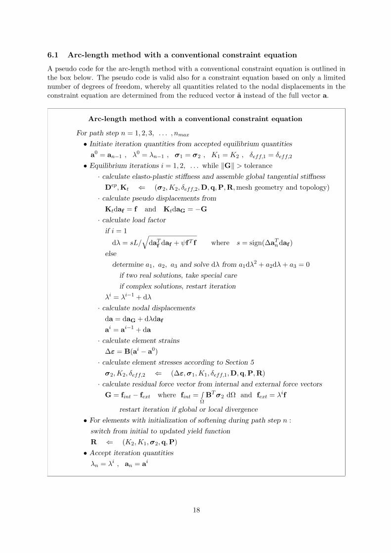
A pseudo code for the arc-length method with a conventional constraint equation is outlined inthe box below. The pseudo code is valid also for a constraint equation based on only a limitednumber of degrees of freedom, whereby all quantities related to the nodal displacements in theconstraint equation are determined from the reduced vector a instead of the full vector a.
Arc-length method with a conventional constraint equation
For path step n = 1, 2, 3, . . . , nmax
• Initiate iteration quantities from accepted equilibrium quantities
a0 = an−1 , λ0 = λn−1 , σ1 = σ2 , K1 = K2 , δeff,1 = δeff,2
• Equilibrium iterations i = 1, 2, . . . while ‖G‖ > tolerance
· calculate elasto-plastic stiffness and assemble global tangential stiffness
Dep,Kt ⇐ (σ2,K2, δeff,2,D,q,P,R,mesh geometry and topology)
· calculate pseudo displacements from
Ktdaf = f and KtdaG = −G· calculate load factor
if i = 1
dλ = sL/√
daTf daf + ψfT f where s = sign(∆aTndaf )
else
determine a1, a2, a3 and solve dλ from a1dλ2 + a2dλ+ a3 = 0
if two real solutions, take special care
if complex solutions, restart iteration
λi = λi−1 + dλ
· calculate nodal displacements
da = daG + dλdaf
ai = ai−1 + da
· calculate element strains
∆ε = B(ai − a0)
· calculate element stresses according to Section 5
σ2,K2, δeff,2 ⇐ (∆ε,σ1,K1, δeff,1,D,q,P,R)
· calculate residual force vector from internal and external force vectors
G = fint − fext where fint = ∫ΩBTσ2 dΩ and fext = λif
restart iteration if global or local divergence
• For elements with initialization of softening during path step n :
switch from initial to updated yield function
R ⇐ (K2,K1,σ2,q,P)
• Accept iteration quantities
λn = λi , an = ai
18

6.2 Arc-length method with a dissipation based constraint equation
A pseudo code for the arc-length method with a constraint equation based on energy dissipationis outlined in the box below. Due to the nature of the constraint equation, being based onconsideration of energy dissipation by plastic straining, the method is only applicable onceplastic straining of the material has taken place. The pseudo code below takes it start in theaccepted equilibrium quantities of path step ndis, during which plastic straining is first initialized.
Arc-length method with a dissipation based constraint equation
For path step n = ndis + 1, ndis + 2, . . . , nmax
• Initiate iteration quantities from accepted equilibrium quantities
a0 = an−1 , λ0 = λn−1 , σ1 = σ2 , K1 = K2 , δeff,1 = δeff,2
• Calculate pseudo force vector
f∗n = ∫ΩBT (Dep)TD−1σ2 dΩ
• Equilibrium iterations i = 1, 2, . . . while ‖G‖ > tolerance
· calculate elasto-plastic stiffness and assemble global tangential stiffness
Dep,Kt ⇐ (σ2,K2, δeff,2,D,q,P,R,mesh geometry and topology)
· calculate pseudo displacements from
Ktdaf = f and KtdaG = −G· calculate load factor
dλ =L− (∆ai−1 + daG)T (λ0f − f∗n)
daTf (λ0f − f∗n)where ∆ai−1 = ai−1 − a0
λi = λi−1 + dλ
· calculate nodal displacements
da = daG + dλdaf
ai = ai−1 + da
· calculate element strains
∆ε = B(ai − a0)
· calculate element stresses according to Section 5
σ2,K2, δeff,2 ⇐ (∆ε,σ1,K1, δeff,1,D,q,P,R)
· calculate residual force vector from internal and external force vectors
G = fint − fext where fint = ∫ΩBTσ2 dΩ and fext = λif
restart iteration if global or local divergence
• For elements with initialization of softening during path step n :
switch from initial to updated yield function
R ⇐ (K2,K1,σ2,q,P)
• Accept iteration quantities
λn = λi , an = ai
19

References
[1] Austrell PE, Dahlblom O, Lindemann J et al. (2004) CALFEM – A finite element toolbox.Version 3.4, Division of Structural Mechanics, Lund University, Sweden.
[2] de Borst R (1987) Computation of post-bifurcation and post-failure behavior of strain-softening solids. Computers and Structures, 25:221-224.
[3] Crisfield MA (1991) Nonlinear finite element analysis of solids and structures – Volume 1.John Wiley & Sons Ltd, Chichester, Great Britain.
[4] Danielsson H, Gustafsson PJ (2013) A three dimensional plasticity model for perpendicularto grain cohesive fracture in wood. Engineering Fracture Mechanics, 98:137-152.
[5] Danielsson H, Gustafsson PJ. Fracture analysis of glulam beams with a hole using a 3Dcohesive zone model.Submitted for publication
[6] Danielsson H, Gustafsson PJ. Fracture analysis of perpendicular to grain loaded dowel-typeconnections using a 3D cohesive zone model.Submitted for publication
[7] Matlab. The Mathworks, Inc.
[8] Ottosen NS, Petersson H (1992) Introduction to the finite element method. Prentice Hall,Great Britain.
[9] Ottosen NS, Ristinmaa M (2005) The mechanics of constitutive modeling. Elsevier, GreatBritain.
[10] Ristinmaa M, Ljung C (1998) An introduction to stability analysis. Division of Solid Me-chanics, Lund University, Sweden.
[11] Tsai SW, Wu EM (1971) A general theory of the strength of anisotropic materials. Journalof Composite Materials, 5:58-80.
[12] Verhoosel CV, Remmers JJC, Gutierrez MA (2009) A dissipation based arc-length methodfor robust simulation of brittle and ductile failure. International Journal for NumericalMethods in Engineering, 77:1290-1321.
20