report: new u.s. power costs: by county, with environmental externalities

The Full Cost of Electricity (FCe-)

New U.S. Power Costs: by County, with Environmental ExternalitiesP a r t o f a s e r i e s o f w h i t e P a P e r s

The Full CosT oF eleCTriCiTy is an interdisciplinary initiative of the Energy Institute of the University of Texas to identify and quantify the full-system cost of electric power generation and delivery – from the power plant to the wall socket. The purpose is to inform public policy discourse with comprehensive, rigorous and impartial analysis.

The generation of electric power and the infrastructure that delivers it is in the midst of dramatic and rapid change. Since 2000, declining renewable energy costs, stringent emissions standards, low-priced natural gas (post-2008), competitive electricity markets, and a host of technological innovations promise to forever change the landscape of an industry that has remained static for decades. Heightened awareness of newfound options available to consumers has injected yet another element to the policy debate surrounding these transformative changes, moving it beyond utility boardrooms and legislative hearing rooms to everyday living rooms.

The Full Cost of Electricity (FCe-) study employs a holistic approach to thoroughly examine the key factors affecting the total direct and indirect costs of generating and delivering electricity. As an interdisciplinary project, the FCe- synthesizes the expert analysis and different perspectives of faculty across the UT Austin campus, from engineering, economics, law, and policy.

In addition to producing authoritative white papers that provide comprehensive assessment and analysis of various electric power system options, the study team developed online calculators that allow policymakers and other stakeholders, including the public, to estimate the cost implications of potential policy actions. A framework of the research initiative, and a list of research participants and project sponsors are also available on the Energy Institute website: energy.utexas.edu

All authors abide by the disclosure policies of the University of Texas at Austin. The University of Texas at Austin is committed to transparency and disclosure of all potential conflicts of interest. All UT investigators involved with this research have filed their required financial disclosure forms with the university. Through this process the university has determined that there are neither conflicts of interest nor the appearance of such conflicts.

This paper is one in

a series of Full Cost

of Electricity white

papers that examine

particular aspects of

the electricity system.

Other white papers

produced through the

study can be accessed

at the University of Texas

Energy Institute website:

energy.utexas.edu

The Full Cost of electricity (FCe-) New U.S. Power Costs: by County, with Environmental Externalities, July 2016 | 1

AbstrAct

In this analysis we developed and applied a geographically-resolved method to calculate the Levelized Cost of Electricity (LCOE) of new power plants on a county-by-county basis while including estimates of some environmental externalities. We calculated LCOE for each county of the contiguous United States for several types of new power plants: coal (bituminous and sub-bituminous, with partial (30%) and full (90%) carbon capture and sequestration), natural gas combined cycle, with and without carbon capture and sequestration) natural gas combustion turbine, nuclear, onshore wind, solar PV (utility and residential), and concentrating solar power (with 6 hours of storage). The new method starts with a conventional LCOE calculation and integrates costs from externalities including air emissions, combustion CO2, and embedded life cycle analysis greenhouse gases. Capital, operating, and fuel costs were spatially interpolated from point locations around the country to each county. Air emissions impacts were included on a county-by-county basis and CO2

costs were applied at the national level. Certain types of power plants were excluded from locations based on various constraints (i.e. water availability for thermal plants, and EPA non-attainment zones for plants that produce air pollutants, etc.). Finally, the method is illustrated by finding the lowest cost option for each county based on different inputs. While the average increased cost for internalizing the environmental externalities is small for some technologies, the local cost differences can be rather high, i.e. $0.05 to $0.62/kWh for coal. We present the results in a map format to facilitate comparisons by fuel, technology, and location. Ten scenarios were considered: a conventional scenario that disregards the costs from environmental externalities, a scenario that includes environmental externalities, a scenario that includes environmental externalities and considers restrictions on where one might be able to site specific technologies, a conventional scenario that disregards the costs from environmental externalities but includes restrictions on siting,

New U.S. Power Costs: by County, with Environmental ExternalitiesA Geographically Resolved Method to Estimate Levelized Power Plant Costs with Environmental Externalities

† Energy Institute, The University of Texas at Austin, Austin, TX‡ Mechanical Engineering, The University of Texas at Austin, Austin, TX¶ Bureau of Economic Geology, Center for Energy Economics,

The University of Texas at Austin, Austin, TX§ Lyndon B. Johnson School of Public Affairs, The University of Texas at Austin, Austin, TXI McCombs School of Business, The University of Texas at Austin, Austin, TX⊥ Center for Electromechanics, The University of Texas at Austin, Austin, TX# Chemicial Engineering, The University of Texas at Austin, Austin, TXE-mail: [email protected]; [email protected]; [email protected]

Joshua D. Rhodes, †,‡

Carey W. King, † Gürcan Gulen, ¶ Sheila M. Olmstead, §

James S. Dyer, I Robert E. Hebner, ⊥ Fred C. Beach, †

Thomas F. Edgar, †, # and Michael E. Webber, †,‡

Rhodes, Joshua D., King, Carey W. Gülen, Gürcan, Olmstead, Sheila M., Dyer, James S., Hebner, Robert E., Beach, Fred C., Edgar, Thomas F., and Webber, Michael E., “A Geographically Resolved Method to Estimate Levelized Power Plant Costs with Environmental Externalities” White Paper UTEI/2016-04-1, 2016, available at http://energy.utexas.edu/the-full-cost-of-electricity-fce/.


scenarios for high and low natural gas prices, scenarios for high and low CO2 prices, a scenario with low solar capital costs, and a scenario using the location’s maximum available onshore wind capacity factor. For nominal reference conditions, the minimum cost option for each county varies based on local conditions and resource available with natural gas combined cycle, wind, and nuclear most often the lowest-cost options. Overall, natural gas combined cycle power plants are the lowest cost option for at least a third of US counties for most cases considered. Wind is also commonly found to be the lowest cost option. Counties where nuclear power is the low-cost option are limited

to locations where natural gas prices are relatively high and wind capacity factors are low. Coal is selected as the low cost option when externalities cost are not high, wind resources are poor, and natural gas prices are high due to distance from existing pipelines. These results, namely that wind and natural gas combined cycle are the most typical low-cost solution, are consistent with recent market trends. These results and display format could serve as an educational tool for stake holders and policymakers when considering which technologies might or might not be a good fit for a given locality subject to system integration considerations.


INTRODUCTION

The levelized Cost of electricity (lCoe) is a commonly used metric for comparing different generation types.

The Levelized Cost of Electricity (LCOE) is typically expressed on a $/kWh basis, it is the estimated amount of money that it takes for a particular electricity generation plant to produce a kWh of electricity over its expected lifetime. LCOE offers several advantages as a cost metric, such as its ability to normalize costs into a consistent format across decades and technology types. Consequently it has become the de facto standard for cost comparisons among the general public and many stakeholders such as policymakers, analysts, and advocacy groups. There are many organizations that calculate LCOE values either for each year,1 future projections,2,3 or for specific clients.4 Despite its advantages and widespread use, the conventional LCOE has several shortcomings that render it spatially and temporally static. Costs of building and operating an identical plant across different geographies will be different. Moreover, fuel costs, capacity factors and financing terms will differ across regions as well. However, LCOE does not readily incorporate these differences, LCOE can also be problematic because of the assumption of constant capacity factors over the lifetime of the plant. Furthermore, the LCOE framework does not anticipate real-time prices or market behaviors, and therefore is more suitable for base load analysis for average conditions. It is also difficult to project LCOE values into the future for fossil fuel and nuclear plants because of the uncertainty of future fuel prices, capacity factors, and regulation. In addition, there have been few attempts to incorporate the costs of environmental externalities into the framework.5–7 We introduce environmental externalities in calculating an expanded LCOE while honoring the spatial variability of emissions and other environmental impacts.

In this paper we present a levelized cost framework that preserves the benefits of the conventional LCOE while adding in environmental externalities and geographic resolution. We start with a standard LCOE calculation and include a few key externalities: SO2, NOx, PM2.5, and PM10 criteria air pollutants emissions; CO2 emissions; and life cycle emissions associated with capital (i.e. steel and concrete) and fuel processing (i.e. uranium enrichment). The criteria air pollutant costs are considered at the county-level based on their marginal impact to human health8 and then internalized into the cost of generating electric energy.9–14 CO2 emissions (upstream, on-going combustion and non-combustion, and downstream) are considered at a national level. In this analysis we consider the following electricity generation types: coal (bituminous and sub-bituminous, partial and “full” CCS), natural gas (combined cycle (NGCC) and combustion turbine (NGCT)), NGCC with CCS, nuclear, onshore wind, solar PV (utility and residential), and concentrating solar power (CSP) with 6 hours of thermal storage. LCOE typically only considers costs that are internal to the plant itself such as capital costs (CAPEX, costs to build the plant itself and any applicable CO2 pipelines, $/kW), debt service costs, fixed Operations and Maintenance costs (O&M, costs associated with the operations and maintenance of the plant, $/MW), variable O&M costs (costs associated with each unit of electricity generated, $/MWh), the heat rate (how much heat it takes to produce a unit of electricity, kJ/kWh (MMBtu/MWh)), the fuel cost (on a per unit of heat basis, $/GJ ($/MMBtu)), and the capacity factor (the amount of energy produced divided by the potential amount of energy that could be produced). However, these aspects vary


by location. This specific analysis incorporates region-specific data on CAPEX, O&M and fuel costs, where available, and uses geographical interpolation techniques to calculate them on a county-by-county basis in the United States.

Other refinements, such as temporal fidelity, levelized avoided cost of electricity (LACE), the impact of subsidies, and the ability to incorporate performance factors (e.g., firming, shaping, storage costs) are not included here but are discussed further in the future work section. Backup and firming costs and other system integration costs such as T&D investments are difficult to incorporate into an LCOE analysis

because these require knowledge of the temporal demand and supply of electricity, which is not natively part of the LCOE equation because these costs are representative of overall electric grid, or system, into which to add a new power plant. This analysis is specifically formulated to show regional differences in the cost of electricity and the results are presented in a series of least-cost county maps. The maps do not imply or suggest rates of technology penetration or regional values associated with any particular market in the US. All costs are in 2015$ USD unless otherwise noted. By definition, our LCOE calculation assumes the marginal addition of one power plant.


METhODS

Our approach is to use the conventional LCOE formulation and then integrate environmental externalities after which the calculations are executed with geographical differentiation. Equation 1 presents the traditional LCOE calculation for which only the plant costs are considered:

CRF = i(1 + i)n

(1 + i)n − 1

eQuATioN 2

eQuATioN 1

LCOE1 = Πcapitalcost × CRF + O&Mfixed + O&M variable + HR × Πf uel8760×CF

eQuATioN 3

LCOE2 = Πcapitalcost × CRF + O&Mfixed + O&M variable + HR × Πf uel8760×CF+ Rj × Dj

j∈θ

For Equation 1, Πcapitalcost is the power plant and any relevant CO2 pipeline overnight capital costs ($/MW), O&Mfixed is the fixed operations and maintenance costs ($/MW), CF is the average capacity factor over the lifetime of the plant, O&Mvariable is the variable operations and maintenance costs ($/MWh), HR is the heat rate (GJ/MWh (MMBtuMWh)), and Πfuel is theprice of fuel ($/GJ ($/MMBtu)). The heat rate and fuel costs are not relevant for wind or solar. CRF is the capital recovery factor, shown in Equation 2:

For Equation 2, i is the interest rate, and n is the number of years to service the debt. Our LCOE calculation inherently assumes the equivalent of borrowing 100% of the capital cost. A modified version integrates the costs of air pollutant emissions. These costs are often considered environmental externalities because they are borne outside the electricity market. Πcapitalcost in Equation 1 includes costs for any required emissions controls (see Section ). Externalities added in Equation 4 reflect the (mostly human health) cost of remaining emissions. Equation 3 presents the LCOE calculation where both the plant costs and the costs associated with SO2, NOx, PM2.5, PM10, and combustion-related CO2 emissions are considered:

where Rj is the rate of emission (tonne/MWh) of pollutant j (see Table 2), Dj is the damages ($/tonne) associated with pollutant j, and θ is a set of pollutants that includes SO2, NOx, PM2.5, PM10,15 CO2,16 and CH4.17 See Table 3 for ongoing CO2 damages per lifetime of power plant. The non-CO2 damages were estimated at the county level as the damage from pollution varies across the nation for a variety of meteorological and other conditions. The damages associated with ongoing CO2 emissions are taken at the national level.

∑


Equation 4 includes the greenhouse gas (GHG) emissions on a carbon dioxide equivalent basis (CO2−eq ) associated with 1) upstream one-time emissions (i.e. building a power plant), on-going non-combustion emissions (i.e. fuel extraction), and 3) downstream one-time emissions (i.e. power plant decommissioning):

+EGHG,one−time × DGHG,one−time

+RGHG,NC,ongoing × DjCO2

eQuATioN 4

LCOE3 = Πcapitalcost × CRF + O&Mfixed + O&M variable + HR × Πf uel8760×CF+ Rj × Dj

j∈θ

where EGHG,one−time are the GHG emissions associated with the one-time upstream and downstream emissions in the construction and decommissioning of a power plant, DGHG,one−time are the damages associated with the one-time upstream and downstream emissions, and RGHG,NC,ongoing is the rate of ongoing non-combustion emissions associated with each technology. Note the values for upstream and downstream emissions damages are different and based on the Social Cost of Carbon corresponding to their year, see Table 3.

While important, we do not consider the cost of water beyond that which is included in O&M costs as water costs have to be relatively high to influence power plant dispatch decisions.18 However, regions with significant water scarcity could have costs from marginal water use high enough to non-trivially affect the overall cost of the power plant. For example, water consumption costs above approximately $1/m3 can incentivize a power plant developer to invest in dry cooling systems to avoid the vast majority of water use.19 We do consider water availability when considering counties that might not be able to support a thermal plant, see the supplementary material.

The end result of this analysis is a modified and expanded LCOE method at the county level. To display this method, we found appropriately spatial data and display the results in map form. Because not all of the data were available at the county level, spatial interpolation methods were used to extend the available data. For instance, EIA calculated the cost ofbuilding power plants in 60 locations across the US. These calculated CAPEX costs were used to interpolate (via the Empirical Bayesian Kriging algorithm in ArcMap 10.2) across all other counties (see Figures 14 – 23). Fixed operating costs (O&Mfixed) were taken from the EIA report and multiplied by the same geographic multipliers as the CAPEX values. Variable operating costs (O&Mvariable) and heat rates for all types of power plants were also taken directly from the EIA report, and were assumed the same across all the regions. A similar approach for fuel prices was used with a starting point of reported delivered fuel costs for fossil plants in their respective counties. Results of these interpolations, along with moredescription are available in the next section. Table 1 shows the assumptions and locations for each type of data used in this analysis.

∑


However, not every type of power plant can be built in every location. Thus, we used maps provided in Mays, et al.22 to determine the availability of locations to build plants based on population density, wetlands, protected lands, lands with landslide risks, highslope land, 100-year floodplains, water availability, EPA non-attainment zones, access to fuel (> 40 km (25 miles) from gas pipelines or railroads), proximity to suitable saline formations for carbon sequestration, and ability to build CO2 pipelines. For each technology the applicable layers were stacked on top of

each other to exclude some counties that have a exclusion factor that significantly decreases the likelihood for constructing a power plant.For instance, it would be more costly to site a thermal power plant in an area that did not have adequate water availability for cooling, or a plant that produces air pollutants in an EPA non-attainment zone, etc. The only plant that did not have an explicit availability zone was residential PV. The exclusion or availability zones for each type of power plant are shown in the supplementary material.

TABle 1

Reference case U.S. average inputs for the considered technologies. Some of the inputs for the reference case are in map format and reference the appendices. For example F14 is a map of county-level coal CAPEX values, F29 is a map of county-level coal capacity factor values located in the supplementary material, and F24 is a map of county-level delivered bituminous coal prices all located in the supplementary material. Individual technology pollutant emissions rates are shown in Table 2. County-level air pollutant damages are taken from Muller and Mendelsohn, Holland et al..15,20

Technology Πcapitalcost O&Mfixed O&Mvariable CF HR Πfuel i n

($/kW)1 ($/kW-yr)2 ($/MWh)3 (%)4 ( kJ )5 ( $ )6 (%)7 (years)7

kW h GJ

Coal, bit CCS 30* 4,766(F14) 49.14 5.81 F29 10,409 3.35(F24) 11% 40Coal, sub CCS 30 4,766(F14) 49.14 5.81 F29 10,409 2.28(F25) 11% 40Coal, bit CCS 90** 5,513(F15) 80.53 9.51 F29 12,661 3.35(F24) 11% 40Coal, sub CCS 90 5,513(F15) 80.53 9.51 F29 12,661 2.28(F25) 11% 40NGCC*** 1,021(F16) 15.37 3.27 F30 6,784 5.37(F26) 10% 35NGCC CCS 90 2,095(F17) 31.79 6.78 F30 7,939 5.37(F26) 10% 35NGCT**** 867(F18) 7.04 10.37 F31 10,287 5.37(F26) 10% 35Nuclear***** 8,000(F19) 93.28 2.14 F32 11,025 0.70 12% 50Wind 1,827(F20) 39.55 0.00 F33 NA NA 10% 25Solar PV, util. 1,900(F21) 24.69 0.00 F34 NA NA 10% 25Solar PV, res. 3,350(F22) 24.69 0.00 F35 NA NA 10% 25CSP 7,041(F23) 67.26 0.00 F36 NA NA 10% 30

* All coal plants are at least partial CCS to bring them into alignment with the EPA’s New Source Performance Standards (Clean Power Plan 111(b)) of 635.6 g/kWh CO2 (1400 lb/MWh), CCS 30: 30% Carbon capture and sequestration.** CCS 90: 90% Carbon capture and sequestration*** Natural gas combined cycle***** Natural gas combustion turbine****** Nuclear heat rate taken from 31 This value is the nominal CAPEX value given in 3 for each technology along with the figure depicting the interpolated

values from the regional multipliers in. 21

2 This value is the nominal fixed operations and maintenance cost value given in 21 for each technology, the values were multiplied by the same interpolated multipliers as the CAPEX values. However, we do not show a regional map of O&M costs for brevity.

3 This value is fixed for all locations for a given technology.4 This value points to the capacity factor map for each technology.5 The heat rate values were assumed constant in all locations for each technology and were taken from. 21 Parametric runs of NGCC and coal-

style boilers in multiple locations across the US indicated negligible differences in heat rates due to climatological differences. The heat rates for different coal types are kept the same with the fuel price reflecting the heat content of the type of coal.

6 This value shows the average fuel price across all locations and also points to the fuel price maps, if applicable.7 Typical interest rates (i) and technology lifetimes (n) for each type were gathered from conversations with utilities.

Rates for CCS plants were left the same as their non-CCS counterparts for lack of available data.


INPUTS fOR ILLUSTRATING ThE METhOD

Overnight capital costs for all plant types were taken from NREL’s 2015 Annual Technology Baseline database.3 CAPEX values for nuclear plants were adjusted up and PV CAPEX values adjusted down based on more recent cost data. Because EPA’s New Source Performance Standards limit the amount of carbon pollution from new power plants to 635.6 g/kWh CO2 (1400 lb/MWh), all new coal plants have to be modeled as CCS plants with at least 30% CO2 capture. Based on23–25 we estimated that 30% CCS increases coal plant CAPEX and OPEX by 30% values and increase in the heat rate by 11% over the EIA/ATB values. These values are reflected in Table 1. Also included in the CAPEX values of CCS plants were costs to build CO2 pipelines of an assumed 100 km length, about $248.6M, or about $2.5M/km ($4M/mile). These costs were then normalized by the assumed capacity of the power plants, 650MW for coal CCS and 340MW for NGCC CCS. CO2 pipe OPEX and CO2 injection well CAPEX and OPEX were normalized by metric tonne of CO2 produced/injected and were calculated to be $4.00, $2.00, and $3.00, respectfully based upon methods used in King et al.,.26

Delivered monthly fuel costs (2007 – 2014) for bituminous coal, sub-bituminous coal, and natural gas were taken from EIA’s 923 form for all reporting natural gas and coal plants in the US. The average fuel price for each county for each type of fuel was then used to spatially interpolate (via the Empirical Bayesian Kriging algorithm in ArcMap 10.2) across all counties that did not have a reporting power plant (see Figures 24 – 26). Fuel costs for nuclear plants were taken constant across all regions at $0.70/GJ.

Five year average capacity factor values for coal, natural gas, and nuclear power plants were gathered from EPA’s Emissions and Generation Resource Integrated Database (eGrid).27 Capacity factors were extracted for each type of plant from the whole database and curated to the NERC subregion level. For lack of data, we assumed that CCS plants had the same capacity factor as their non-CCS counterparts. These values are actual reported historical capacity factors for each

type of plant (see Figures 29 – 32). Historical capacity factors are used because capacity factors are driven by markets and regulatory structures as well as the technology. Thus, we assume that the dispatch for a given technology would be roughly the same as current plants of the same technology. While fuel prices will affect capacity factor, EIA data indicate that the average price for natural gas has been at about the same price we are using, thus we feel comfortable using historical capacity factors. Capacity factor valuesfor on-shore wind were obtained from 3Tier at a 5km×5km resolution28 and were averaged at the county level. Wind capacity factors would be higher and thus the LCOE lower if the best locations in each county were chosen for siting the wind turbine. The capacity factor values were for a generic turbine with a hub height of 80m (Figure 33). Capacity factor values for utility and residential-scale solar PV plants were calculated using the capacity factor maps found in Drury et al., 2013.29 Because these maps were at a finer granularity than county-level, the average value per county was calculated. Utility-scale PV was assumed to be single-axis tracking and residential PV was assumed to be south-facing fixed-tilt at the local latitude (see Figures 34 – 35). Capacity factor values for solar CSP were calculated using NREL’s System Advisory Model (SAM).30 Weather data from over 1000 locations across the US were used with the SAM model of a generic concentrating solar plant with 6 hours of thermal energy storage. The resulting capacity factors for the plants were then used to give each county in the US a CSP capacity factor based on similar meteorological conditions (Figure 36).

EIA emissions rates of SO2, NOx, and CO2 for each type of power plant were used for each technology. The EIA emissions rates assume that the plant contains the Best Available Commercial Technology (BACT). Thus these emissions controls technologies that are part of BACT are reflected in CAPEX values. Table 2 summarizes our cited non-combustion, life cycle emissions associated with each type of power plant31 and our assumed combustion rates for air pollutants.


Damages for CO2 and CO2−eq emissions were calculated using the EPA’s Social Cost of Carbon (SCC).16 The lifetime of each power plant type is different (Table 1), and thus thedamages associated with upstream, ongoing, and downstream emissions were also treated differently. Table A1 of16 presents calculated average annual social cost of carbon values for 2010–2050 for discount rates of 5, 3, and 2.5%. In this analysis, the 3% average rates were used as the reference case and the 2.5% and 5% discount rates were used as the high and low cost cases, respectfully. Because our nuclear plants had an assumed life of 50 years and we start at 2015, we extrapolated the values in Table A1 of16 to 2065 using a 2nd degree polynomial fit to extrapolate the data past its current end, the R2 was > 99% in each case. Marten and Newbold, 201217 showed that using the SCC with other gasses’ global warming potential could lead to errors in estimating the societal cost of those gasses. Because we consider the impact that fugitive methane emissions have on the cost of electricity from natural gas plants, we calculated damages from emissions using the Social Cost of Methane (SCM).17 Table 3 shows the final values for the SCC and the SCM used for the LCOEcalculations.

County-level marginal emissions damages (adjusted to 2015$) for SO2, NOx, PM2.5, were taken from.20 PM10 values were taken from Mueller and Mendelsohn, 2009.15 Both15,20 provided ground level, intermediate, and high stack emissions costs, mainly associated with increased morbidity and mortality, for each type of pollutant on a county-level basis. We use the intermediate values in our calculations, though the framework of the modified LCOE could be used with the high and low range values too. However, there is some difference between the two datasets. The SO2, NOx, PM2.5 data from20 are based on a $6M value of a statistical life (VSL) with 2011 as the base year of emissions. The PM10 data are from an earlier study with a base year of 2002,15 and used a VSL of $2M, scaled by age – thus a low estimate for PM10 as compared to the study using a $6M VSL. These estimates were held constant throughout the analysis period because although air quality has improved in many locations which reduces the impact of a marginal tonne of emissions, healthcare costs continue to rise, so the future movement of these damage estimates is uncertain. Figure 1 portrays a graphical flow of the data streams used to display our method.

Technology Upstream one-time (g CO2−eq /kW )

On-going non-combustion (g CO2−eq /kW h)1

Downstream one-time

(g CO2−eq /kW )

CombustionSO2

CombustionNOx

CombustionPM10

CombustionPM2.5

CombustionCO2

Fugitive CH42

Coal CCS 30* 257,000 48 15,200 0.4 0.24 0.327 0.268 635.6 0Coal CCS 90** 385,500 72 22,800 0.4 0.24 0.327 0.268 82.1 0NGCC*** 160,000 74.4 6,390 0.003 0.022 0.054 0.05 341.5 1.58

NGCC CCS 90 240,000 111.6 9,585 0.003 0.022 0.054 0.05 35 1.85

NGCT**** 6,800 85.8 98.6 0.005 0.133 0.054 0.05 517.9 2.39Nuclear 350,000 10.6 175,000 0 0 0 0 0 0Wind 619,000 1.41 22,400 0 0 0 0 0 0Solar PV 1,630,000 0 37,800 0 0 0 0 0 0CSP 2,970,000 2.5 239,000 0 0 0 0 0 0

* CCS 30: 30% Carbon capture and sequestration** CCS 90: 90% Carbon capture and sequestration*** NGCC: Natural gas combined cycle**** NGCT: Natural gas combustion turbine1 The values for natural gas units assume a US average natural gas infrastructure leakage rate of 2.5%, see the supplementary information.2 Assuming a US average methane leakage rate of 1.0%.

TABle 2

Table showing the assumed life cycle emissions rates (g/kW(h)) of CO2−eq (GHG), the assumed BACT combustion emissions rates (g/kWh) of air pollutants, and the assumed CH4 fugitive emissions rates (g/kWh) associated with the considered technologies.


TABle 3

Table 3: Table showing the low, reference, and high case assumptions for the cost of ongoing CO2 (combustion and non-combustion) and CH4 (fugitive emissions) damages ($/tonne) for plant lifetimes of 25, 30, 35, 40 and 35 years, damages associated with upstream or 2015 emissions, and damages associated with downstream emissions for the same plant lifetimes.

FiGure 1

Figure showing the flow of data from raw inputs to county-level LCOE calculations.

Timeline Low* Reference** High***

Ongoing (25 yr) $18 $58 $83Ongoing (30 yr) $19 $60 $85Ongoing (35 yr) $20 $62 $88Ongoing (40 yr) $22 $65 $91Ongoing (50 yr) $25 $71 $98Upstream (today, 2015) $14 $43 $65Downstream (25 yr) $24 $71 $98Downstream (30 yr) $27 $75 $105Downstream (35 yr) $31 $81 $111Downstream (40 yr) $35 $88 $117Downstream (50 yr) $44 $99 $129

Ongoing CH4 (35 yr)1 $1,034 $2,014 $2,562

* 5% discount rate** 3% discount rate*** 2.5% discount rate1 All natural gas power plants were assumed a lifetime of 35 years, so only this value is shown here.


RESULTS

We applied the method for multiple scenarios to demonstrate how it could be used. Figure 2 (Scenario 1) shows the minimum cost technology for each county in a scenario where we do not consider externalities or availability zones. That is, the LCOE of each technology was calculated using Equation 1, and the minimum cost technology for each county is shown. In this scenario, our method, using numbers we describe in Section finds that in the majority of US counties, NGCC plants are the least cost option, followed by wind, sub bituminous coal and nuclear plants. Again, these costs do not include any investment or production tax credits, loan guarantees, property tax abatements, depletion allowances, fuel price hedging schemes, or firming costs.Figure 3 shows the underlying LCOE cost of the minimum cost technology in every county shown in Figure 2. The bottom of Figure 3 shows the distribution of LCOE values for each technology relative to each other. For instance the distribution shows us that there is considerable overlap in the cost distribution for NGCC and

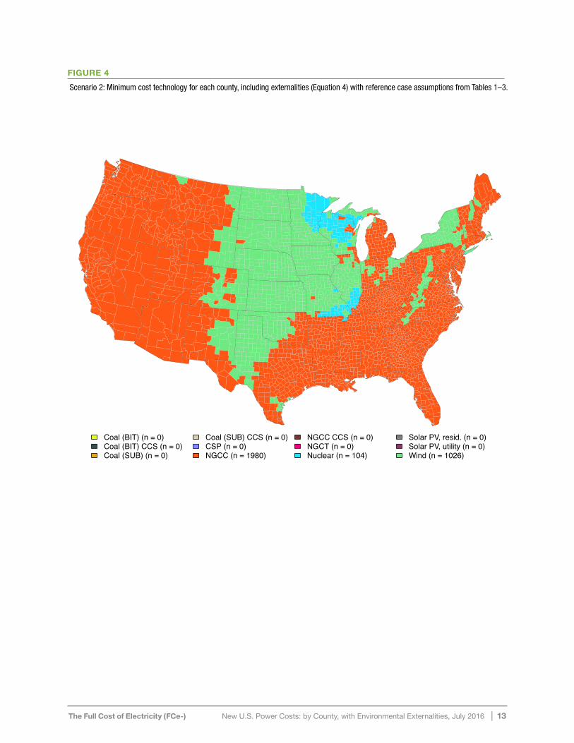
Wind plants, but the bulk of the NGCC plants cost less than the bulk of Wind plants. The figure also shows an inset of the most expensive plants in this scenario for ease of viewing.Figure 4 (Scenario 2) shows the minimum cost technology for each county in a scenario where we do consider externalities, but not availability zones. That is, the LCOE of each technology was calculated using Equation 4, and the minimum cost technology for each county is shown. In this scenario, our method finds that in the majority of US counties, NGCC plants are still the least cost option, followed by increased wind and nuclear plants, but coal is no longer the least cost option in any county when externalities are considered.

Figure 5 shows similar LCOE values and distribution results for Figure 4 as discussed above.

Figure 6 (Scenario 3) shows the minimum cost technology for each county in a scenario where we consider both externalities and availability zones (see the supplementary information).

Scenario 1: without availability zones and without externalities

Coal (BIT) (n = 0)Coal (BIT) CCS (n = 0)Coal (SUB) (n = 29)

Coal (SUB) CCS (n = 0)CSP (n = 0)NGCC (n = 2316)

NGCC CCS (n = 0)NGCT (n = 0)Nuclear (n = 23)

Solar PV, resid. (n = 0)Solar PV, utility (n = 0)Wind (n = 742)

FiGure 2 __

Scenario 1: Minimum cost technology for each county, not including externalities (Equation 1) with reference case assumptions from Tables 1–3.


FiGure 3:

Scenario 1 LCOE map (top) showing the LCOE value for the minimum cost technology for each county, not including externalities (Equation 1) with reference case assumptions from Tables 1–3. The distribution plot (bottom) shows the distribution of the cost of each technology relative to each other.

Scenario 1 LCOE $/kWh

0.050

0.059

0.068

0.077

0.086

0.095

0.104

0.113

0.122

0.131

0.140

LCOE ($/kWh)

0

50

100

150

200

Freq

uenc

y

0.05 0.1 0.15 0.2 0.25 0.3 0.35 0.4 0.45

Coal (BIT) (n = 0)Coal (BIT) CCS (n = 0)Coal (SUB) (n = 29)Coal (SUB) CCS (n = 0)

CSP (n = 0)NGCC (n = 2316)NGCC CCS (n = 0)NGCT (n = 0)

Nuclear (n = 23)Solar PV, resid. (n = 0)Solar PV, utility (n = 0)Wind (n = 742)










0

5

10

15

0.12 0.14


Scenario 2: without availability zones and with externalities





FiGure 4

Scenario 2: Minimum cost technology for each county, including externalities (Equation 4) with reference case assumptions from Tables 1–3.



0.06

0.07

0.08

0.09

0.10

0.11

0.12

0.13

0.14

0.15

0.16

LCOE ($/kWh)

0

50

100

150

Freq

uenc

y

0.05 0.1 0.15 0.2 0.25 0.3 0.35 0.4 0.45










FiGure 5

Scenario 2 LCOE map (top) showing the LCOE value for the minmum cost technology for each county, including externalities (Equation 4) with reference case assumptions from Tables 1–3. The distribution plot (bottom) shows the distribution of the cost of each technology relative to each other.


Scenario 3: with availability zones and externalities





FiGure 6

Scenario 3: Minimum cost technology for each county, including externalities (Equation 4) and availability zones with reference case assumptions from Tables 1–3.

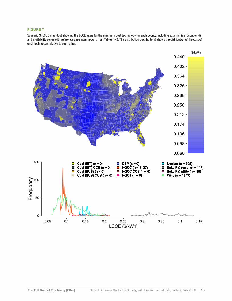
Figure 7 shows similar LCOE values and distribution results for Figure 6 as discussed above.

Of all fuel and technology combinations considered, local least-cost option in a county is highly dependent on locality. In locations where the wind resource is strong and/or barriers (non-attainment zones, water availability, etc.) are high for thermal plants, wind tends to be the lowest-cost option. In Figure 6, our method indicates that wind is the lowest cost option in the most number of counties. NGCC is the least cost option in counties where the wind resource isn’t as strong. Nuclear plants are the least-cost technology where wind resources are marginal and gas prices are high, or natural gas pipelines are not available. Residential solar PV plants are the default

option when a county was otherwise excluded by one or more barriers to other technologies. Utility-scale solar PV plants are more clustered in locations that have excellent solar insolation levels and/or lack of cooling water availability. NGCT plants are located where conditions are also favorable to NGCC plants, but lack cooling water availability. The average reference case cost for all the counties’ minimum cost technologies was $0.127/kWh (median: $0.102/kWh).

Figure 8 shows the minimum cost technology per county when availability zones are considered, but externalities are given a price of zero. Because Scenarios 4–10 are iterations of Scenario 3, we do not show the LCOE values map and distributions for them.



0.060

0.098

0.136

0.174

0.212

0.250

0.288

0.326

0.364

0.402

0.440

LCOE ($/kWh)

0

50

100

150

Freq

uenc

y

0.05 0.1 0.15 0.2 0.25 0.3 0.35 0.4 0.45



















FiGure 7

Scenario 3: LCOE map (top) showing the LCOE value for the minimum cost technology for each county, including externalities (Equation 4) and availability zones with reference case assumptions from Tables 1–3. The distribution plot (bottom) shows the distribution of the cost of each technology relative to each other.


Scenario 4: with availability zones and without externalities





FiGure 8

Scenario 4: Minimum cost technology for each county, including availability zones, but not including externalities (Equation 1) with reference case assumptions from Table 1.

Figure 8 (Scenario 4) shows the minimum cost technology for each county in a scenario where we do not consider externalities, but do include availability zones. For this scenario, as compared to Figure 6, there are more counties where there lowest LCOE is a fossil-fueled power plant, and fewer counties with wind and nuclear plants. Along the edges of the wind corridor (where the wind is of less quality than the interior) wind farms, which were the lowest cost option when environmental externalities are included, are replaced by NGCC plants where water is available, and NGCT and PV where it is not. For a considerable number of locations in the southeast where nuclear was the least-cost option in Scenario 3 utility-scale PV is the least-cost option in Scenario 4. This change is due to PV’s highupstream GHG values (see Table 2) from

fabrication of the panels. When the cost of the externalities are not internalized, PV is lower cost. The average cost for the case that did not consider externalities was $0.103/kWh (median: $0.080/kWh). The costs of air emissions (for coal about $0.03/kWh, not including CO2) are for additional marginal emissions from a new plant with Best Available Commercial Technology.21 These values should not be used as a proxy to estimate the benefit of removing an existing plant. If we instead use emissions rates from existing plants (average emissions rates in NERC subregions via eGrid27), the emissions costs are, on average, about 10 times higher. This difference is highly dependent on location; some counties have older coal plants with limited emission control equipment whereas others do not have a coal plant that could be removed.Prices for natural gas, coal, and nuclear fuel vary


Scenario 5: Scenario 3 with a high gas price





FiGure 9

Scenario 5: Minimum cost technology for each county, including externalities (Equation 4) and availability zones with reference case assumptions from Tables 1–3 with a high natural gas price (US average of $7/MMBtu, Figure 28).

over time. Generators can stabilize prices via long-term contracts or financial hedges but cannot fully avoid price risk. Of those fuels, natural gas price has been most volatile over the last 15–20 years. The volatility of the natural gas price contributes to temporal variation in wholesale electricity market prices as it is often the marginal generation fuel. Hence, it is valuable to analyze the sensitivity of gas plants’ LCOE to reasonable low and high prices. In Figure 10 (Scenario 5), we see the effect of lower ($3/MMBtu, Figure 27) and in Figure 9 (Scenario 6), we see the effect of higher ($7/MMBtu, Figure 28) natural gas prices. High and low natural gas price methodologies

and maps are explained in later sections of this supplementary material. Note that we do not adjust the capacity factor of NGCC and NGCT plants based on the price of natural gas.

In comparison to Scenario 3 (Figure 6), the primary effect of higher or lower natural gas prices is switching between wind and NGCC: when natural gas prices are higher, wind becomes the low-cost option in many counties in which NGCC is the low-cost option in the reference case; when natural gas prices are lower, NGCC becomes the low-cost option for many counties in which wind is the low-


Scenario 6: Scenario 3 with a low gas price





FiGure 10

Scenario 6: Minimum cost technology for each county, including externalities (Equation 4) and availability zones with reference case assumptions from Tables 1–3 with a low natural gas price (US average of $3/MMBtu, Figure 27).

cost option in Scenario 3. We also examined the effect of a lower (Scenario 7) and higher (Scenario 8) CO2 price in Figures 11 and 12. The values of CO2 are based on the EPA’s Social Cost of Carbon and are different based on plant life expectancy and assumed discount rates. For more explanation of these values, see Table 3 and the corresponding section.

In the case of higher CO2 prices (Figure 11); wind, nuclear, and coal CCS plants increase while natural gas, coal, and utility-scale PV plants decrease. Again utility-scale PV decreases because of the high upstream GHG values for PV plants. In the case of

lower CO2 prices (Figure 12), the opposite happens.

In scenario 9 (Figure 13), we consider the impacts of solar installers achieving the U.S. Department of Energy’s SunShot goal of $1/Watt (or $1,000/kW) for installed CAPEX of utility-scale PV and $1.5/Watt (or $1,500/kW) for installed CAPEX of residential PV.32

In scenario 9, both forms of solar PV increase in the number of locations where they are the lowest-cost option. Solar PV displaces most of the locations in Scenario 3 where nuclear was the least cost option. Solar PV does displace some wind and NGCC plants, but the relative percent changes are not as drastic for these technologies.


Scenario 7: Scenario 3 with a high CO2 price





FiGure 11

Scenario 7: Minimum cost technology for each county, including externalities (Equation 4) and availability zones with reference case assumptions from Tables 1–3 with a high price on all forms of CO2 (Table 3).

This result affirms the idea that if policymakers wish to see growth in the market penetration of solar energy, then it is important to pursue policies that reduce the capital costs. This scenario does not imply that the electric system could operate with 100% solar power in any part of the country. It simply states that, given current conditions, $1/W ($1.5/W) utility (residential) solar would be the least cost technology in many locations if the current system could accommodate it without any need for backup or firming costs. In scenario 10, we use the maximum capacity factor for onshore wind in each county (Figure 14).The resolution for wind capacity factor was obtained on a 5-km grid for the entire United States. Thus, most counties included more than one

value for wind capacity factor that was averaged for that county for use in our reference case. In some large counties, particularly in the western United States, the average wind capacity factor can be up to 38% less than the maximum in that county. Using the maximum wind capacity factor rather than average capacity factor significantly increases the number of counties where the minimum cost technology is wind. In fact, the effect of using the maximum wind capacity factor is similar to that of a high carbon cost – many of the locations that switch to wind (from the reference case) are the same as those in the high carbon scenario.This analysis gives the ability to see the spatial differences of the costs of each technology across the entire United States. Because capital and


Scenario 8: Scenario 3 with a low CO2 price





FiGure 12

Scenario 8: Minimum cost technology for each county, including externalities (Equation 4) and availability zones with reference case assumptions from Tables 1–3 with a low price on all forms of CO2 (Table 3).

operating costs (labor, etc.), fuel price, emissions damages, and capacity factors, among other factors, vary across regions, so does the levelized cost of electricity. Some factors not considered in this analysis could also impact local prices. If reliability factors are internalized, wind and solar might be more costly because of their variability. However this need is highly dependent on local grid conditions and penetration levels. Other factors, such as fuel disposal, further fuel price volatility, and water use could also have local cost impacts on fossil fuel plants. If thermal power plants operate with higher capacity factors, then their costs would be lower and they would be selected as the low-cost option for more counties. Wind would be selected in more counties if only the best sites within each county is used.

SECOND MINIMUM COST TEChNOLOGy

Figure 15 shows the next least cost technology map for all United States counties (top) as well as the cost difference between the least and second least cost technology on the bottom. The distribution between technologies is distributed among all the technologies except for solar with nuclear having the greatest number counties as the second least cost technology. The average difference between the first and second least cost technology for all locations is $0.029/kWh.


Scenario 9: Scenario 3 using SunShot solar CAPEX goals





FiGure 13

Scenario 9: Minimum cost technology for each county, including externalities (Equation 4) and availability zones with reference case assumptions from Tables 1–3 with a lower installed cost: $1/W for utility-scale solar PV and $1.5/W for residential PV.


Scenario 10: Scenario 3 with the max wind capacity factor per county





FiGure 14

Scenario 10: Minimum cost technology for each county, including externalities (Equation 4) and availability zones with reference case assumptions from Tables 1–3 using the maximum capacity factor in each county for onshore wind.


Reference case second minimum cost technology





Second minimum technology cost difference $/kWh

0.00

0.02

0.04

0.06

0.08

0.10

0.12

0.14

0.16

0.18

0.20

Reference case second minimum cost technology





Second minimum technology cost difference $/kWh

0.00

0.02

0.04

0.06

0.08

0.10

0.12

0.14

0.16

0.18

0.20

FiGure 15

Map showing the second minimum cost technology for each county (Equation 4) with reference case assumptions from Table 1 on top and the cost difference between the least and next least cost technology on the bottom. A lighter color on the bottom graph indicates a smaller difference between the first and second least cost technology.


CONCLUSIONS

This analysis presents 1) a spatially-resolved method to internalize variations in construction costs and air and GHG emissions of electricity production for multiple types of fuel and technologies, and 2) a geographic display of the method for 10 scenarios. Data were compiled to a county-by-county basis and interpolated when necessary. The internalization of factors that are traditionally not considered is important for policy decisions that seek to reduce environmental impacts in an economically efficient way. Geographic emphasis is also important, because the best technology decision is different depending on the location. We also find that when the minimum technology cost (including externalities) is found for each county, natural gas combined cycle, wind, and nuclear power are all the least-cost option the most frequently, but are sensitive to natural gas and carbon prices.

fUTURE wORkFuture work can include such aspects as firming power, transmission and distribution upgrades, impacts to terrestrial and aquatic biodiversity, and a full accounting for the value of water used in thermal plants. The costs developed in this analysis will be used in dispatch and capacity expansion models to incorporate time-of-use pricing and market dynamics.

DISCLOSURE Of AffILIATIONAll authors abide by the disclosure policies of the University of Texas at Austin. The University of Texas at Austin is committed to transparency and disclosure of all potential conflicts of interest. All UT investigators involved with this research have filed their required financial disclosure forms with the university. None of the researchers have reported receiving any research funding that would create a conflict of interest or the appearance of such a conflict.

In addition to research work on topics generally related to energy systems at the University of Texas at Austin, some of the authors are equity partners in IdeaSmiths LLC, which consults on topics

in the same areas of interests. The terms of this arrangement have been reviewed and approved by the University of Texas at Austin in accordance with its policy on objectivity in research.

A full list of sponsors for all projects in Dr. Webber’s research group at UT are listed at http://www.webberenergygroup.com/about/sponsors/. Dr. Webber’s affiliations and

board positions are listed at http://www.webberenergygroup.com/people/michael-webber/. Dr. King’s sponsors can be viewed on his website at http://careyking.com/projects/.

Dr. Edgar’s sponsors can be viewed on this website http://energy.utexas.edu/mission/ sponsors-financial-support/. Current/recent Center for Energy Economics sponsors are listed at http://www.beg.utexas.edu/energyecon/partnrs.php.

ACkNOwLEDGEMENTThis project was principally funded by UT Austin’s Energy Institute, which receives support from academic units on the UT Austin campus engaged in energy research, as well as unrestricted financial contributions from a variety of industrial, governmental and non-profit sponsors. Visit www.energy.utexas.edu/sponsors for additional details. We would like to acknowledge Austin Energy, City Public Service Energy, Sharyland Utilities, the Cynthia and George Mitchell Foundation, Chevron, and the Environmental Defense Fund for their financial support and intellectual contributions to this study. In addition, we would like to thank the American Wind Energy Association, ConocoPhillips, FirstSolar, NRG, and AEP, the National Renewable Energy Lab, and Oak Ridge National Lab for their technical inputs. This acknowledgement should not be considered an endorsement of the results by any of the entities that contributed financially or intellectually. The authors would also like to thank Yuval Edrey for his help with data analysis.


REfERENCES

(1) Lazard, Lazard’s levelized cost of energy analysis, Version 8.0. 2014; www.lazard.com.

(2) EIA, Annual Energy Outlook 2014. 2014; http://www.eia.gov/forecasts/aeo/pdf/ 0383(2014).pdf.

(3) Sullivan, P. et al. 2015 Standard Scenarios Annual Report: U.S. Electric Sector Scenario Exploration; 2015.

(4) Black and Veatch, Cost and Performance data for Power Generation Technologies; 2012; pp 1–106.

(5) Cohon, J. L. Hidden costs of energy: unpriced consequences of energy production and use; The National Academies Press: Washington, DC, 2010; p 653.

(6) Epstein, P. R.; Buonocore, J. J.; Eckerle, K.; Hendryx, M.; Stout, B. M.; Heinberg, R.; Clapp, R. W.; May, B.; Reinhart, N. L.; Ahern, M. M.; Doshi, S. K.; Glustrom, L. Full cost accounting for the life cycle of coal. Annals of the New York Academy of Sciences 2011, 1219, 73–98.

(7) Wittenstein, M.; Rothewll, G. Projected Costs of Generating Electricity, 2015th ed.; International Energy Agency: Paris, France, 2015; p 215.

(8) Buonocore, J. J.; Dong, X.; Spengler, J. D.; Fu, J. S.; Levy, J. I. Using the Community Multiscale Air Quality (CMAQ) model to estimate public health impacts of PM2.5 from individual power plants. Environment International 2014, 68, 200–208.

(9) Cullen, J. Measuring the Environmental Benefits of Wind-Generated Electricity. American Economic Journal: Economic Policy 2013, 5, 107–133.

(10) McCubbin, D.; Sovacool, B. K. Quantifying the health and environmental benefits of wind power to natural gas. Energy Policy 2013, 53, 429–441.

(11) Kaffine, D. T.; McBee, B. J.; Lieskovsky, J. Emissions Savings from Wind Power Generation in Texas. The Energy Journal 2013, 34 .

(12) Novan, K. Valuing the Wind: Renewable Energy Policies and Air Pollution Avoided. American Economic Journal: Economic Policy 2015, 7, 291–326.

(13) Siler-Evans, K.; Azevedo, I. L.; Morgan, M. G.; Apt, J. Regional variations in the health, environmental, and climate benefits of wind and solar generation. Proceedings of the National Academy of Sciences 2013, 110, 11768–11773.


(14) Shindell, D. T. The social cost of atmospheric release. Climatic Change 2015, 130, 313–326.

(15) Muller, N. Z.; Mendelsohn, R. Efficient Pollution Regulation: Getting the Prices Right. American Economic Review 2009, 99, 1714–1739.

(16) Technical Update of the Social Cost of Carbon for Regulatory Impact Analysis. 2013; https://www.whitehouse.gov/sites/default/files/omb/inforeg/social_cost_of_carbon_for_ria_2013_update.pdf.

(17) Marten, A. L.; Newbold, S. C. Estimating the social cost of non-CO 2 GHG emissions: Methane and nitrous oxide. Energy Policy 2012, 51, 957–972.

(18) Sanders, K. T.; Blackhurst, M. F.; King, C. W.; Webber, M. E. The Impact of Water Use Fees on Dispatching and Water Requirements for Water-Cooled Power Plants in Texas. Environmental Science & Technology 2014, 48, 7128–7134.

(19) King, C. W., Ed. Thermal Power Plant Cooling: Context and Engineering, 1st ed.; ASME, 2014; p 264.

(20) Holland, S.; Mansur, E.; Muller, N.; Yates, A. Environmental Benefits from Driving Electric Vehicles? 2015; http://www.nber.org/papers/w21291.pdf.

(21) EIA, Updated Capital Cost Estimates for Utility Scale Electricity Generating Plants. 2013; http://www.eia.gov/forecasts/capitalcost/pdf/updated{_}capcost.pdf.

(22) Mays, G. T.; Belles, R. J.; Blevins, B. R.; Hadley, S. W.; Harrison, T. J.; Jochem, W. C.; Neish, B. S.; Omitaomu, O. A.; Rose, A. N. Application of Spatial Data Modeling and Geographical Information Systems (GIS) for Identification of Potential Siting Options for Various Electrical Generation Sources; 2012.

(23) Hildebrand, A. N. Strategies for Demonstration and Early Deployment of Carbon Capture and Storage: A Technical and Economic Assessment of Capture Percentage. Ph.D. thesis, Massachusetts Institute of Technology, 2009.

(24) Chou, V.; Iyengar, A. K.; Shah, V.; Woods, M. Cost and Performance Baseline for Fossil Energy Plants. 2015; https://www.netl.doe.gov/FileLibrary/Research/ EnergyAnalysis/Publications/BitBase{_}Partial{_}Capture{_}final.pdf.

(25) Supekar, S. D.; Skerlos, S. J. Reassessing the Efficiency Penalty from Carbon Capture in Coal-Fired Power Plants. Environmental Science & Technology 2015, 49, 12576–12584.

(26) King, C. W.; Gülen, G.; Cohen, S. M.; Nuñez-Lopez, V. The system-wide economics of a carbon dioxide capture, utilization, and storage network: Texas Gulf Coast with pure CO2-EOR flood. Environmental Research Letters 2013, 8, 034030.

(27) eGrid. 2015; http://www.epa.gov/cleanenergy/energy-resources/egrid/.


(28) 3Tier, Wind Energy Project Feasibility. 2015; http://www.3tier com/en/products/ wind/project-feasibility/.

(29) Drury, E.; Lopez, A.; Denholm, P.; Margolis, R. Relative performance of tracking versus fixed tilt photovoltaic systems in the USA. Progress in Photovoltaics: Research and Applications 2013, 22, 1302–1315.

(30) NREL, System Advisor Model (SAM). 2015; https://sam.nrel.gov.

(31) Mai, T.; Wiser, R.; Sandor, D.; Brinkman, G.; Heath, G.; Denholm, P.; Hostick, D. J.;

(32) Darghouth, N.; Schlosser, A.; Strzepek, K. Volume 1: Exploration of High-Penetration Renewable Electricity Futures. Renewable Electricity Futures Study 2012, 1, 280.

(33) Margolis, R.; Coggeshall, C.; Zuboy, J. Sunshot Vision Study. 2012; http://www1. eere.energy.gov/solar/pdfs/47927.pdf.

report: new u.s. power costs: by county, with environmental externalities

News & Politics