report 1 4 - fate of dispersed oil under ice · ms. ragnhild lundmark daae, sintef materials and...
TRANSCRIPT

Page 1
24 October 2013 Dr. CJ Beegle-Krause Dr. Harper Simmons, University of Alaska, Fairbanks Dr. Miles McPhee, McPhee Research Company Ms. Ragnhild Lundmark Daae, SINTEF Materials and Chemistry Dr. Mark Reed, SINTEF Materials and Chemistry
LITERATURE REVIEW: FATE OF DISPERSED OIL UNDER ICE FINAL REPORT 1.4 Literature Review – Fate of Dispersed Oil Under Ice
Literature Review: Fate of Dispersed Oil Under Ice
2
ABOUT THE JIP
Over the past four decades, the oil and gas industry has made significant advances in being able to detect, contain and clean up spills in Arctic environments. To further build on existing research, increase understanding of potential impacts of oil on the Arctic marine environment, and improve the technologies and methodologies for oil spill response, in January 2012, the international oil and gas industry launched a collaborative four-year effort – the Arctic Oil Spill Response Technology Joint Industry Programme (JIP).
Over the course of the programme, the JIP will carry out a series of advanced research projects on six key areas: dispersants, environmental effects, trajectory modeling, remote sensing, mechanical recovery and in situ burning. Expert technical working groups for each project are populated by the top researchers from each of the member companies.
JIP MEMBERS
The JIP is managed under the auspices of the International Association of Oil and Gas Producers (OGP) and is supported by nine international oil and gas companies – BP, Chevron, ConocoPhillips, Eni, ExxonMobil, North Caspian Operating Company (NCOC), Shell, Statoil, and Total – making it the largest pan-industry programme dedicated to this area of research and development.

Literature Review: Fate of Dispersed Oil Under Ice
3
TABLE OF CONTENTS
ABOUT THE JIP ........................................................................................................................................................ 2
JIP MEMBERS ........................................................................................................................................................... 2
EXECUTIVE SUMMARY ........................................................................................................................................... 5
CHAPTER 1. INTRODUCTION .............................................................................................................................. 7
CHAPTER 2. UNDER ICE TURBULENCE AND CURRENTS, OBSERVATIONS AND METHODS ................... 8 Existing Measurements ............................................................................................................................. 8 2.1
2.1.1 Measurements under Thick, Multiyear Ice ................................................................................ 9
2.1.2 IOBL Measurements in the Marginal Ice Zone (MIZ) ............................................................. 11
2.1.3 IOBL Measurements under Thin, First-Year Pack Ice ............................................................. 12
2.1.4 IOBL Measurements under Fast Ice in Tidal Regimes ........................................................... 12
2.1.5 IOBL Measurements from Unmanned, Drifting Buoys .......................................................... 13
2.1.6 Microstructure Measurements in the Pycnocline and Deep Ocean ..................................... 13
Ice and Sea State Conditions in Areas of Oil Development and High Vessel Traffic ........................ 14 2.22.2.1 Natural Ice and Sea State Conditions ..................................................................................... 14
2.2.2 Frazil, Slush and Shuga Ice ....................................................................................................... 15
2.2.3 Rough Ocean (Pancake Cycle) ................................................................................................. 15
2.2.4 Calm Ocean (Congelation growth) ......................................................................................... 15
2.2.5 Ice Deformation ........................................................................................................................ 16
2.2.6 Wind Stress Transfer through Ice ............................................................................................ 16
2.2.7 Ice Growth and Melt ................................................................................................................. 17
2.2.8 Relevance for Turbulence and Fate of Oil Droplets .............................................................. 17
2.2.9 Oil-in-Ice Field Experiments .................................................................................................... 18
2.2.10 Ice Regimes ............................................................................................................................... 18
Under Ice Turbulence Measurement Techniques ................................................................................. 19 2.32.3.1 Turbulence Instrument Clusters (TICs) .................................................................................... 19
2.3.2 Shear Microstructure ................................................................................................................ 20
2.3.3 Scalar Microstructure ................................................................................................................ 21
2.3.4 Acoustic Doppler Velocimetry and Current Profilers (ADCPs) .............................................. 22
2.3.5 Passive Tracers .......................................................................................................................... 23
2.3.6 Particle Image Velocimetry (PIV) and LASER Doppler Velocimetry (LDV) ............................ 24
Summary and Recommendations ........................................................................................................... 24 2.4
CHAPTER 3. MODELS ......................................................................................................................................... 27 Turbulent Transport Modeling in the Ice-Ocean Boundary Layer ....................................................... 27 3.1
3.1.1 Model Classes, Review of Model Types Applied to the IOBL .............................................. 27
3.1.2 Turbulent Fluxes, TKE, Scales of Turbulence, and First-Order Closure ............................... 29
3.1.3 Ocean Drag on Sea Ice: Rossby Similarity .............................................................................. 32
3.1.4 Scalar Exchange at the Ice/Ocean Interface: Viscous Sub-Layers ........................................ 33
3.1.5 Inertial Oscillations and Internal Waves .................................................................................. 34
Analogous Systems in Dispersion and Transport Modelling ............................................................... 36 3.23.2.1 Oil Droplet Turbulent Mixing: State-of-the-Art ...................................................................... 36
3.2.2 Simple Mixing ........................................................................................................................... 37
3.2.3 Chemical and Radionuclide Transport .................................................................................... 37
3.2.4 Atmospheric Dispersion Models ............................................................................................. 37
Literature Review: Fate of Dispersed Oil Under Ice
4
3.2.5 Sediment and Suspended Particulate Matter (SPM) Transport ............................................ 38
Modeling Gaps ........................................................................................................................................ 39 3.33.3.1 Oil Droplets in a Turbulent IOBL ............................................................................................. 39
3.3.2 Oil in the Near-Shore, Ice Infested Environment ................................................................... 39
3.3.3 Impact of Oil at the Ice/Water Interface ................................................................................. 41
3.3.4 The Marginal Ice Zone .............................................................................................................. 42
3.3.5 Changing Ocean Circulation in the Arctic .............................................................................. 43
Summary ................................................................................................................................................... 44 3.4
CHAPTER 4. OVERALL SUMMARY, ANALYSIS AND RECOMMENDATIONS ............................................... 45 Turbulence Model Selection ................................................................................................................... 46 4.1 Model Input Requirements ..................................................................................................................... 47 4.2 Prioritization of Ice Types in Field Study ................................................................................................ 47 4.3
CHAPTER 5. REFERENCES ................................................................................................................................. 49
Literature Review: Fate of Dispersed Oil Under Ice
Executive Summary 5
EXECUTIVE SUMMARY
The fate of a cloud of oil droplets under ice depends essentially on the droplet size distribution, the vertical turbulence profile, and the horizontal transport field. The longer the droplets are retained in the water column, the more the droplet cloud will become diluted due to horizontal mixing, and the more the oil will biodegrade. Oil droplets that resurface under the ice will also not tend to reform into larger slicks or pools, to the extent that the average inter-droplet distance exceeds the mean horizontal distance between under-ice roughness elements.
This literature review supports the view that sufficient knowledge exists to develop an under-ice turbulence closure model, but that existing observations are probably not good enough to provide both calibration and verification data. The mixing of oil droplets in nature differs significantly from the dispersion of ichthyoplankton and other nearly neutrally buoyant particles and tracers. Surfacing oil droplets change character to sheens and slicks. These require energy to disperse back into the water column, and the resulting droplet sizes may in general not be the same as those that created the surface expression.
There are a number of possible observational strategies for obtaining new data to support development and calibration of an under-ice turbulence model. For pack or drift ice characterized by large stable floes, turbulent instrument clusters (TICs) remain the workhorse instrument package. Caveats include the fact that such environments could be extremely spatially heterogeneous so that a relatively small number of TICs might not adequately sample the small-scale variability of turbulence regimes near ridges and keels. Powered AUVs are potentially an ideal platform for measuring turbulence in the Ice-Ocean Boundary Layer (IOBL), particularly when combined with measurements of ice draft with sonar. Autonomous Underwater Vehicles (AUVs) have the ability to survey spatially and allow investigators to respond to observed spatial and temporal changes in the met-ocean-ice environment. They could potentially be deployed in a broad range of ice concentrations provided adequate vessel support was available. The downside is that the instrumentation is costly and risks can be high. Also, AUVs cannot sample into the log-layer very close to the water-ice boundary that may be important for oil spreading and local enhancement of turbulence. Note however that powered AUV operations in heavy ice cover are becoming more routine, with under-ice topography from single or multi-beam sonar an essential component of the operations. Also note that multi-beam sonar data from an AUV has previously been combined with flow modeling to predict the spread of oil under fast ice.
Ice exists in a wide variety of ice types, morphologies, and characteristics: thickness, degree of coverage, floe size, porosity, and so forth. The major categories of ice are discussed briefly within this report. To the extent that these differences contribute to changes in the under-ice turbulence profile for a given met- ocean (wind-current-wave) regime, the differences are relevant to the problem being addressed here. There are many possible observational strategies for improving and evaluating our ability to model the fate potential for an oil patch to remain suspended in the water column which will be determined by the particular ice-regime of interest along with other environmental parameters as well as cost and personnel safety. Below is a short list based on successful field studies in the past.
Fluorescent Dyes Turbulent Instrument Cluster (TIC) Autonomous Underwater Vehicles Acoustic Doppler Current Profilers (ADCPs) Passive traces such as flourescene and rhodamine
Literature Review: Fate of Dispersed Oil Under Ice
Executive Summary 6
Based on the literature review, careful selection of the turbulence closure model and environmental input data (i.e. currents and waves) are keys to predictive success. The literature of particle simulations in Eulerian flows covers a wide range of topics, from larval fish, oil and other contaminants, intentional tracer releases, sediments and SPM. The model provided is expected to be valid in greater than 90% ice cover, as the IOBL will continue to behave as if ice covered, and perhaps as low as 75% ice cover. There is potential to be valid at even lower ice coverage, as experience during the AIDJEX experiment shows ice cover as low as 25% was only different in the absorption of solar radiation.
No off-the-shelf model exists that can be easily adapted to the variety of ice types and concentrations that could be encountered during a spill where oil dispersal (chemical or mechanical) is required. Adaptation of the McPhee (2008) first order Local Turbulence Closure (LTC) model based on the literature review . Our reasoning is as follows:
LTC is based on combining turbulence similarity theory with extensive direct measurements of turbulence characteristics in the under ice boundary layer under widely varying conditions of ice types and physical forcing (stress, heat and salt fluxes).
In contrast to slab (mixed-layer) models, a model incorporating LTC provides vertical profiles of turbulence properties critical for determining the fate of oil droplets in the water column: Reynolds stress, buoyancy flux, eddy viscosity/diffusivity, as well as total kinetic energy (TKE) production and dissipation. LTC and K-profile parameterization (KPP) 1st order closures include the high shear region near the interface explicitly, rather than considering it separately. It is important that shear in the outer part of the IOBL is acknowledged since it means oil will be transported in quite different directions depending on distance from the boundary.
An LTC model also provides realistic vertical velocity profiles that are fundamentally shaped by rotational (Coriolis) forces, critical for determining the speed and direction of droplet motion at different levels in the water column.
Real-time forecast implementation of LTC is relatively straightforward. An on-board model incorporating meteorological forecasts and ice-concentration imagery was used daily with good results during the MaudNESS project in the Weddell Sea, Antarctica, and has been included as part of a major tracer-tracking experiment proposed for the Arctic (IDEAr).
LTC is readily adaptable to specific local conditions including energetic inertial oscillation (cycloidal ice motion), shallow environments with or without stratification, complications posed by frazil generation, and/or sediment transport.
Observations collected must be made in the presence of oil droplets in the water column, which can interfere with some instrumentation. We expect the following measurements could be made on a spill response timescale:
Wind Droplet size distribution (noted as a given by the TWG) Ice Type -> proxy for bottom roughness Ice Concentration Turbulence Profile Velocity Profile
From the input data above, the final model would provide guidance on the likelihood of oil resurfacing. In planning the field program and details of the model development we may determine we need to collect additional field data alongside the above listed parameters to ensure that the implemented model is fully calibrated and functional.
Literature Review: Fate of Dispersed Oil Under Ice
Introduction 7
CHAPTER 1. INTRODUCTION
Oil spill response in the presence of sea ice is potentially both more complex and more simple than in open water. In higher concentrations of sea ice, the oil will in general spread less rapidly, but may be more difficult to intercept either mechanically or with other response strategies such as dispersant application or in situ burning. In this project we are interested in developing a model to identify conditions in which chemical or mechanical dispersal will be successful in removing oil permanently from the sea surface. This is a concern because the vertical turbulence that successfully keeps small oil droplets in suspension in open water may be significantly reduced under ice fields due to wave damping.
The project will progress in two phases, with this first phase providing a summary of background information on the state of knowledge concerning under-ice turbulence, potential gaps therein, and methods for obtaining additional data as necessary to allow the development of a reliable model to predict whether oil droplets could surface within a two day period based upon an initial oil droplet size distribution.
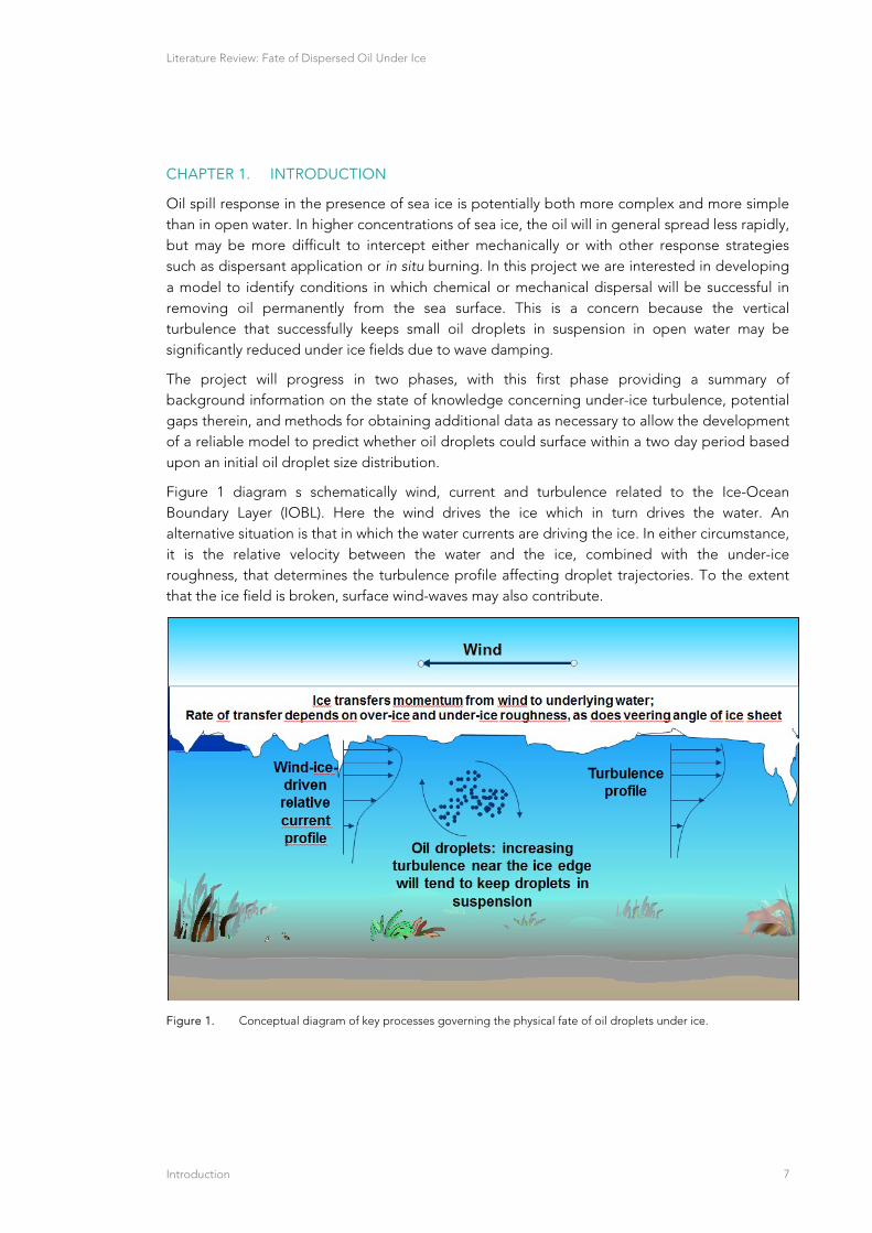
Figure 1 diagram s schematically wind, current and turbulence related to the Ice-Ocean Boundary Layer (IOBL). Here the wind drives the ice which in turn drives the water. An alternative situation is that in which the water currents are driving the ice. In either circumstance, it is the relative velocity between the water and the ice, combined with the under-ice roughness, that determines the turbulence profile affecting droplet trajectories. To the extent that the ice field is broken, surface wind-waves may also contribute.
Figure 1. Conceptual diagram of key processes governing the physical fate of oil droplets under ice.
Literature Review: Fate of Dispersed Oil Under Ice
Under Ice Turbulence and Currents, Observations and Methods 8
CHAPTER 2. UNDER ICE TURBULENCE AND CURRENTS, OBSERVATIONS AND METHODS
Existing Measurements 2.1
Experiments staged from sea ice are responsible for the majority of what we know about turbulent transfer of momentum and scalar contaminants (including heat and salt) from direct observation in planetary boundary layers (PBLs). The reasons for this are straightforward. An ocean covered by ice presents a solid upper boundary that quells surface gravity waves, eliminating or reducing orbital wave velocities and providing a solid platform from which to suspend instruments that remain relatively stationary to an observer on the ice. Although turbulence measurements in the lower tens of meters of the atmosphere are common, turbulence and boundary layer scales are roughly 30 times as large as in the ocean, making measurements technically challenging in the outer (Ekman) part of the boundary layer (~100 to 1000 m) except by instrumented aircraft.
A cornerstone of turbulence theory is that turbulent energy generated by large scale, low wavenumber instabilities (“energy-containing eddies”) in a sheared flow “cascades” to smaller and smaller scales until dissipated as heat by molecular viscosity. As discussed in more detail in Chap. 2, the key to describing this process is the turbulent kinetic energy (TKE) equation and the TKE spectrum expressed in angular wavenumber space ( 2 ⟨ ⟩⁄ where is frequency in cps). Essentially, spectral density peaks at wavenumbers representing the scale of the largest eddies, and vanishes near scales identified by Kolmogorov dependent on the rate of TKE dissipation, ԑ, and the kinematic molecular viscosity. In between these scales is a region called
the inertial sub-range where the spectral density is proportional to ԑ2/3k‐5/3. Standard texts treating turbulence include Batchelor (1967), Hinze (1975), and Tennekes; Lumley (1972a).
In the ocean, root-mean square turbulent velocities at the low wavenumber end of the turbulence spectrum (largest turbulent scales) are at most a few centimeters per second. By eliminating platform motion and wave velocities, the “fluid laboratory” provided by sea ice makes feasible measurements of the small turbulent velocities needed to estimate fluxes directly via Reynolds averaging (calculating covariances) and the “frozen-field” hypothesis relating time series covariances of the fluctuating flow and scalar components to ensemble turbulent averages. For example, the horizontal traction vector caused by the vertical momentum flux is
⟨ ⟩ ⟨ ⟩ , (0.1)
where brackets are averages and primes denote the velocity in each direction after removal of the mean, e.g., ⟨ ⟩. Similarly, for a scalar like heat the vertical flux, Hf, follows from the covariance of temperature and vertical velocity
⟨ ⟩ (0.2)
where and are density and specific heat of seawater, respectively. In order to adequately
measure these fluxes (i.e., capture most of the covariance) in the ice/ocean boundary layer (IOBL) requires resolving turbulence scales into the inertial sub-range, thus we look for a turbulent energy spectrum with a -5/3 slope in log-log representation. Note that the covariance method for estimating fluxes approaches the TKE cascade from the low wavenumber part of the spectrum.

Literature Review: Fate of Dispersed Oil Under Ice
Under Ice Turbulence and Currents, Observations and Methods 9
In a wave-influenced boundary layer, small turbulent fluctuations are embedded in much higher orbital wave velocities with enough energy to dominate the velocity spectrum. Consequently, turbulence studies in the ocean with no ice cover often concentrate on measuring at very small scales (high wavenumber end of the spectrum) with so-called microstructure instruments, then estimating ԑ by integrating empirical fits to the shear (velocity gradient) spectra at very small scales (Gregg et al. 1986; Moum et al. 1995). Given estimates of ε and corresponding estimates of χ, the dissipation of temperature variance, flux magnitudes are derived from consideration of the production terms in the TKE and variance conservation equations, along with knowledge of vertical gradients. Although this technology is relatively mature (Lueck et al. 2002) and has provided much useful data on exchange in stratified fluids (see section 1.1.7), its application in a wave-dominated regime with extremely small gradients (typical of the well mixed layer) is problematic from several standpoints, including angle-of-attack issues and the frozen field hypothesis in an oscillating current regime (Gerbi et al. 2009); Fer and Paskyobi, submitted).
In the following subsections we review IOBL turbulence measurements made in a wide variety of ice types and forcing conditions. Theoretical underpinnings of the IOBL theory, and many of the measurements included below, are described in more detail by McPhee et al. (2008).
2.1.1 Measurements under Thick, Multiyear Ice
The majority of published data on turbulence in the IOBL have been collected under relatively thick, multiyear, drifting pack ice, beginning with the Arctic Ice Dynamics Joint Experiment Pilot Study in 1972. For that experiment Professor J. D. Smith of the University of Washington deployed masts with triads of small mechanical current meters oriented along orthogonal axes, providing high-resolution, three-dimensional currents at scales well into the inertial sub-range of the turbulence spectrum, hence providing for the first time direct measurement of the turbulent Reynolds stress tensor ( ⟨ ′ ′⟩) at multiple levels through an entire planetary
boundary layer. The trace of is the kinematic turbulent stress tensor, which is twice the TKE
per unit mass. That initial study established the observational basis for addressing several characteristics of the ice-ocean boundary layer (IOBL), and provided a template for subsequent studies. From the Pilot Study, McPhee; Smith (1976) analysed data from two storm events to show that in the IOBL the so-called logarithmic layer extended at most a few meters from the boundary and that at lower levels, the “outer” layer behaved pretty much as Ekman had predicted, including dependence of eddy viscosity on boundary stress. Their measurements of TKE through the entire IOBL corresponded closely with numerical atmospheric boundary layer models that were just beginning to appear at the time (Wyngaard 1975; Wyngaard et al. 1974), including the first application of large-eddy simulation (LES) modelling (Deardorff 1974). They also found that velocity integrated over the entire IOBL (volume transport) was perpendicular to stress at the surface, a strikingly clear manifestation of the importance of rotation (Coriolis force) in IOBL dynamics.
The 1984 Marginal Ice Zone Experiment (MIZEX) north of Fram Strait was aimed at understanding ice behaviour near the edge of the ice pack in the Greenland Sea (section 1.1.2), but one component was a ship-supported drift station sited on a multiyear floe that started in conditions representative of the typical interior summer ice pack, with IOBL temperature near freezing, and slow basal melt rates. For MIZEX, Smith’s basic current-meter triad idea was expanded to include fast response temperature and conductivity sensors (Sea-Bird Electronics) mounted near the current meters in the same horizontal plane in a turbulent instrument cluster (TIC) configuration. An inverted mast with TICs at several levels provided robust measurements
Literature Review: Fate of Dispersed Oil Under Ice
Under Ice Turbulence and Currents, Observations and Methods 10
of vertical turbulent heat flux for the first time in the ocean, in addition to documenting the turbulent stress tensor at several levels (Morison et al. 1987).
During a pair of projects under the Coordinated Eastern Arctic Experiment (CEAREX) in the fall of 1987 and spring of 1988 (Cearex_Drift_Group 1990), TICs were again deployed as arrays in the IOBL. During the spring program, a drift station was deployed on the northwest flank of Yermak Plateau in an ocean regime unlike others encountered elsewhere in the Arctic ice pack. Internal tides along the slope of the plateau produced energetic bores (Padman et al. 1992) that carried large scale, breaking internal waves that apparently added to the turbulent energy of the IOBL (McPhee 1992a, 1994b; McPhee; Martinson 1994). For CEAREX the TIC system was revised to include a modified Sea-Bird Electronics (SBE) 9 CTD, mounted on a rigid mast with 5 TICs that could be lowered to as much 100 m below the surface.
In 1992, two projects utilizing the turbulence instrument clusters (TICs) added greatly to the IOBL turbulence knowledge base. Ice Station Weddell was a joint US/Russian ice station deployed in multiyear ice in the western Weddell Sea (Antarctica), drifting roughly parallel to Shackleton’s 1915-1916 drift of the Endurance (Gordon et al. 1993). Data recorded from a mast with TICs mounted 4 m apart through the entire IOBL revealed an unmistakable Ekman spiral in turbulent stress, from measurements at five different levels. By careful cross-calibration of the SBE temperature sensors when heat flux was near zero, an independent measure of eddy thermal diffusivity was obtained by dividing the average measured turbulent heat flux in the IOBL by the negative temperature gradient that agreed well with various methods of estimating eddy viscosity (McPhee 1994b; McPhee; Martinson 1994).
The Arctic Leads Dynamic Experiment (LeadEX), also in 1992, comprised a main station deployed on multiyear ice in the Canada Basin that supported four exercises during which a wide range of instrumentation was transported to the edges of newly opened leads via helicopter or snow machine (LeadEx_Group 1993). Based on earlier observations (some resulting from fortuitous ice camp breakups), the important role that leads played in the Arctic IOBL was clear (Dasaro; Morison 1992), thus LeadEX was designed to gauge response of the upper ocean and atmosphere to rapid freezing. Novel features of LeadEX included complementary simultaneous TIC and microstructure measurements in a forced convective upper ocean regime (McPhee; Stanton 1996), and convective turbulence measured by an autonomous underwater vehicle (Morison; McPhee 1998).
As its title suggests, the year-long Surface Heat Budget of the Arctic (SHEBA) experiment (1997-98) was a major interdisciplinary project aimed at elucidating the various components of the energy budget that determines the mass balance of sea ice (Uttal et al. 2002). Oceanographic measurements in all seasons included a TIC mast as in earlier experiments plus a continuously profiling CTD/microstructure instrument. In the summer (1998), freshwater storage and mixing1 across open leads was investigated with an autonomous underwater vehicle (Hayes; Morison 2002). Included in the extensive scientific findings from SHEBA relating to ice/ocean exchanges are:
1 We use the word mixing in the chapter to distinguish between dispersion as the breakup of an oil slick into droplets and the vertical and horizontal mixing of those droplets in the water column. Spreading is also sometimes used in the context, but we will use the term spreading to denote the oil at the water's surface that is thinning and spreading out in area.

Literature Review: Fate of Dispersed Oil Under Ice
Under Ice Turbulence and Currents, Observations and Methods 11
(i) the dominant source of heat during summer was incoming solar radiation absorbed by the upper ocean, then transferred to the ice base via turbulence in the IOBL (Shaw et al. 2009);
(ii) the dimensionless mean bulk heat transfer coefficient was 0.0057 0.0004 (McPhee et al.2003);
(iii) the mean value of under-ice hydraulic roughness was estimated at log 3.0 1.0, with a mean value of 0.049 m (McPhee et al. 2008);
(iv) first estimates of vertical transport of turbulent kinetic energy in the IOBL (McPhee 2004); and
(v) abrupt pycnocline upwelling (apparently caused by extreme local ice shearing) with intense turbulent transfer of heat and salt into the IOBL from below (McPhee et al. 2005).
Data from the SHEBA experiment have been widely incorporated into parameterizations of physical processes for large scale ice/ocean models (Kay et al. 2011). Worth noting is that SHEBA occurred toward the beginning of widespread appreciation of changes occurring in the Arctic (McPhee 1998b; Rothrock et al. 1999), which have accelerated since these earlier studies (McPhee 2013; McPhee et al.2009).
Turbulence instrumentation was also deployed during the austral summer of 2004-2005 during the Ice Station Weddell Polar Experiment (ISPOL) from an ice station supported by R/V Polarstern situated on multiyear ice (with several icebergs within view) in the western Weddell Sea, again not far from the drift track of the Endurance. A combination of turbulence measurements and acoustic Doppler current
profiler (ADCP) data provided the basis for a novel method of estimating the overall roughness of the heterogeneous ice floe to which the ship was moored, as well as confirming the dominant role of rotation in determining turbulence scales close to the ice-ocean boundary at low stress levels (McPhee 2008a).
2.1.2 IOBL Measurements in the Marginal Ice Zone (MIZ)
In the 1980s a series of experiments was directed toward understanding the complex air-ice-ocean interactions in the transition zones from the open ocean to its ice-covered state (Johannessen et al. 1983; McPhee 1983a; Mizex_Group 1989; Muench 1983). Sharp density gradients and volume transport divergence (Ekman pumping) drive complex fronts, current jets, and eddies along the MIZ (Buckley et al. 1979; Paquette; Bourke 1979, 1981).
High melt rates in water more than a few tenths of a degree above its freezing temperature are found almost exclusively in MIZs, since ice cannot survive long in those conditions. Toward the end of the 1984 MIZEX drift, the ice station crossed over a sharp MIZ front into water more than a degree above freezing. Direct turbulent heat flux measurements combined with ice ablation data gathered then formed the basis for understanding the double-diffusive character (different transfer rates for heat and salt) of the melting interface (McPhee et al. 1987; Morison et al. 1987), completely revising its parameterization in ice/ocean models (see Chap. 2). Measurements during rapid melting also elucidated the impact of stabilizing buoyancy flux on turbulence scales in the IOBL (McPhee 1994a). More recently, Sirevaag (2009) used heat, salt, and momentum flux in the MIZ north of Svalbard to make the first direct estimates of interface exchange coefficients for heat and salt, confirming the role of double diffusion. After crossing the MIZ front during a period of moderate wind stress, the MIZEX floe slowed, allowing stratification to develop up to the ice/water interface. Then during the last two days of the project as wind picked up, ocean drag increased from earlier values while heat transfer
Literature Review: Fate of Dispersed Oil Under Ice
Under Ice Turbulence and Currents, Observations and Methods 12
decreased. Morison et al. (1987) interpreted this as momentum flux directly into the internal wave field, thus reducing energy available for scalar mixing. McPhee; Kantha (1989) corroborated their interpretation by modelling work incorporating a “lee-wave” mechanism into the IOBL force balance (Gill 1982) that becomes important when pressure ridge keels occupy a sizable portion of the well mixed layer depth.
Some of the highest values for hydraulic roughness of the ice underside have been reported for ice in the MIZ (Johannessen 1970; McPhee et al. 1987; Pease et al. 1983), as a result of floe fragmentation and deformation associated with rapid attenuation and energy loss from surface gravity waves (Squire 1995; Wadhams et al. 1988).
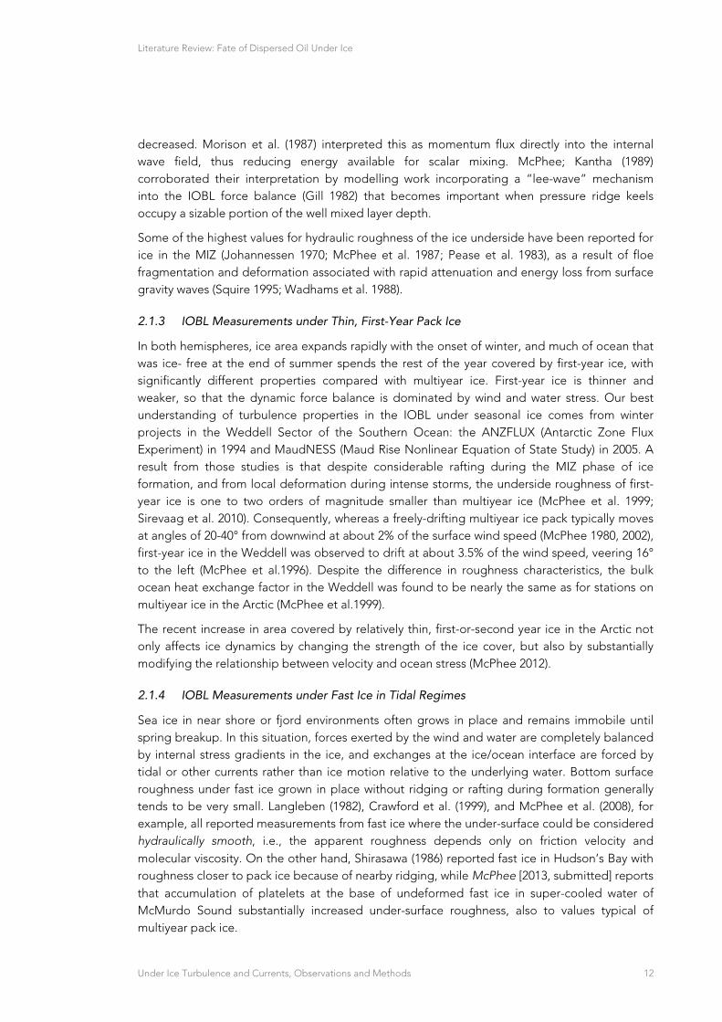
2.1.3 IOBL Measurements under Thin, First-Year Pack Ice
In both hemispheres, ice area expands rapidly with the onset of winter, and much of ocean that was ice- free at the end of summer spends the rest of the year covered by first-year ice, with significantly different properties compared with multiyear ice. First-year ice is thinner and weaker, so that the dynamic force balance is dominated by wind and water stress. Our best understanding of turbulence properties in the IOBL under seasonal ice comes from winter projects in the Weddell Sector of the Southern Ocean: the ANZFLUX (Antarctic Zone Flux Experiment) in 1994 and MaudNESS (Maud Rise Nonlinear Equation of State Study) in 2005. A result from those studies is that despite considerable rafting during the MIZ phase of ice formation, and from local deformation during intense storms, the underside roughness of first-year ice is one to two orders of magnitude smaller than multiyear ice (McPhee et al. 1999; Sirevaag et al. 2010). Consequently, whereas a freely-drifting multiyear ice pack typically moves at angles of 20-40° from downwind at about 2% of the surface wind speed (McPhee 1980, 2002), first-year ice in the Weddell was observed to drift at about 3.5% of the wind speed, veering 16° to the left (McPhee et al.1996). Despite the difference in roughness characteristics, the bulk ocean heat exchange factor in the Weddell was found to be nearly the same as for stations on multiyear ice in the Arctic (McPhee et al.1999).
The recent increase in area covered by relatively thin, first-or-second year ice in the Arctic not only affects ice dynamics by changing the strength of the ice cover, but also by substantially modifying the relationship between velocity and ocean stress (McPhee 2012).
2.1.4 IOBL Measurements under Fast Ice in Tidal Regimes
Sea ice in near shore or fjord environments often grows in place and remains immobile until spring breakup. In this situation, forces exerted by the wind and water are completely balanced by internal stress gradients in the ice, and exchanges at the ice/ocean interface are forced by tidal or other currents rather than ice motion relative to the underlying water. Bottom surface roughness under fast ice grown in place without ridging or rafting during formation generally tends to be very small. Langleben (1982), Crawford et al. (1999), and McPhee et al. (2008), for example, all reported measurements from fast ice where the under-surface could be considered hydraulically smooth, i.e., the apparent roughness depends only on friction velocity and molecular viscosity. On the other hand, Shirasawa (1986) reported fast ice in Hudson’s Bay with roughness closer to pack ice because of nearby ridging, while McPhee [2013, submitted] reports that accumulation of platelets at the base of undeformed fast ice in super-cooled water of McMurdo Sound substantially increased under-surface roughness, also to values typical of multiyear pack ice.
Literature Review: Fate of Dispersed Oil Under Ice
Under Ice Turbulence and Currents, Observations and Methods 13
Tidal currents in enclosed bays and fjords often advect horizontal gradients in temperature and salinity with large impact on the scales and intensity of mixing. Velocity shear near the fast ice (upper) boundary will create transient vertical density gradients. At cold temperatures, density depends almost exclusively on salinity, so as a salinity front passes a fixed site, if fresher water replaces saltier, turbulence will be enhanced because the flow of saltier water near ice/water boundary is retarded, creating an unstable vertical density gradient. On the opposite phase, denser water under-runs lighter, and turbulence is reduced. Examples have been reported by Crawford et al. (1999) and McPhee et al. (2013). Examples have been reported by Crawford et al. (1999) and (McPhee et al. 2013).
2.1.5 IOBL Measurements from Unmanned, Drifting Buoys
The introduction of clusters of sophisticated ocean buoys equipped with ice properties, profiling and turbulence instrumentation, with near real-time data transmission by Iridium satellite telemetry is revolutionizing our ability to sample the Arctic Ocean (Krishfield et al. 2008; Timmermans et al. 2011). An example of using turbulence and hydrographic data from buoys deployed in a cluster, to estimate area-averaged under-surface roughness in highly deformed ice is presented by Shaw et al. (2008). The ice-tethered profiler program from Woods Hole has recently tested a buoy with a three-dimensional, travel time ultrasonic current meter that shows promise of enhancing the already very valuable ITP data stream (Cole et al. 2012)
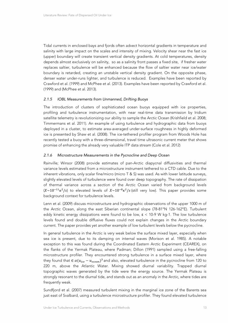
2.1.6 Microstructure Measurements in the Pycnocline and Deep Ocean
Rainville; Winsor (2008) provide estimates of pan-Arctic diapycnal diffusivities and thermal variance levels estimated from a microstructure instrument tethered to a CTD cable. Due to the inherent vibrations, only scalar fine/micro (micro T & S) was used. As with lower latitude surveys, slightly elevated levels of turbulence were found over deep topography. The rate of dissipation of thermal variance across a section of the Arctic Ocean varied from background levels ( ~10 / ) to elevated levels of ~10 / (still very low). This paper provides some background context for turbulence levels.
Lenn et al. (2009) discuss microstructure and hydrographic observations of the upper 1000 m of the Arctic Ocean, along the east Siberian continental slope (78-81°N 126-162°E). Turbulent eddy kinetic energy dissipations were found to be low, ε < 10-9 W kg-1. The low turbulence levels found and double diffusive fluxes could not explain changes in the Arctic boundary current. The paper provides yet another example of low turbulent levels below the pycnocline.
In general turbulence in the Arctic is very weak below the surface mixed layer, especially when sea ice is present, due to its damping on internal waves (Morison et al. 1985). A notable exception to this was found during the Coordinated Eastern Arctic Experiment (CEAREX), on the flanks of the Yermak Plateau, where Padman; Dillon (1991) sampled using a free-falling microstructure profiler. They encountered strong turbulence in a surface mixed layer, where they found that ∈ and also, elevated turbulence in the pycnocline from 120 to 220 m, above the Atlantic Water. Mixing showed diurnal variability. Trapped diurnal topographic waves generated by the tide were the energy source. The Yermak Plateau is strongly resonant to the diurnal tide, and stands out as an anomaly in the Arctic, where tides are frequently weak.
Sundfjord et al. (2007) measured turbulent mixing in the marginal ice zone of the Barents sea just east of Svalbard, using a turbulence microstructure profiler. They found elevated turbulence
Literature Review: Fate of Dispersed Oil Under Ice
Under Ice Turbulence and Currents, Observations and Methods 14
associated with shear layers and tides. Mixing levels between the base of the mixed layer and the pycnocline were strongly enhanced at many of their stations with ∈ 1 1010 ⁄ associated with eddy diffusivities of 1 10 10 . Mixing due to internal waves was effectively modeled using a parameterization by MacKinnon; Gregg (2003) using approximately 10m scale shear and strain measurements from ADCPs and conventional CTDs.
During the Arctic Internal Waves Experiment (AIWEX) Padman; Dillon (1987) performed hundreds of microstructure profiles using micro-conductivity and shear probes. Data was gathered in the Canada Basin in the depth interval between 300 and 420m. Throughout the experiment, turbulence levels were at the noise floor of the instrument, approximately 10 ⁄ .Scalar fluxes were dominated by double- diffusive fluxes through thermohaline staircases, the presence of which support the finding that turbulence was essentially zero in this layer.
Fer et al. (2010) measured turbulence on a shallow shoulder of the Yermak Plateau at 5 stations using a microstructure profiler. Data was collected in the upper 500 meters where water depths were sufficient. At this site turbulence was approximately 0.1 to 0.3 times mid-latitude levels, which is weak, but similar to other measurements in the Arctic.
Ice and Sea State Conditions in Areas of Oil Development and High Vessel Traffic 2.2
The Arctic sea ice extent has been decreasing during the last five decades (Arctic Council, 2009), and the polar ice is projected to be about 50% ice-free during the summer months by 2080 (Zhang & Walsh, 2006). Models are underestimating the rate of perennial sea ice loss (Stroeve et al., 2007) and the opening up of Arctic Seas during summer for both transportation of goods and oil exploration. A decreasing perennial ice pack is occurring together with increasing ice drift and deformation rates (Rampal et al., 2009). This may increase the hazard of encountering poorly detectable older ice in the expanding seasonal ice zone of the Western Arctic. Ice drift also preconditions the ice pack for summer melt (Rigor and Wallace 2004, Hutchings et al. 2012), expanding the seasonal ice zone in the Western Arctic, decreasing ice thickness and opening new regions for exploration.
There are a variety of ice and sea state conditions which are encountered in the Arctic. We consider the different types and stages of development of sea ice relevant for modelling of the fate and effects of oil spills:
During initial freeze-up, oil can freeze into the sea ice, be transported with the ice drift, and be released elsewhere when melting occurs;
The marginal ice zone, where conditions vary rapidly in both space and time;
Drifting ice with low ice concentration;
Medium ice concentrations,
Pack ice with high ice concentration, where oil is contained/trapped between the ice floes and moves with the ice field
2.2.1 Natural Ice and Sea State Conditions
The types and stage of development of sea ice are described by WMO (1970) terminology (see for example MANICE 2005). We describe sea ice characteristics, specific to regions were modelling is of interest, considering ice and sea state that may be encountered.
Literature Review: Fate of Dispersed Oil Under Ice
Under Ice Turbulence and Currents, Observations and Methods 15
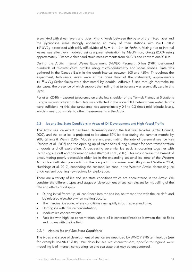
There are two branches of ice growth processes. One branch originates during rough seas, and the other during calm seas. The first one is often referred to as the "Pancake cycle", and the other as "Congelation growth". These two cycles are described in Table 1 .
Table 1. Description of the ice growth process
Stage Pancake cycle Congelation growth
Young ice Frazil ice Pancake ice rafting Frazil ice Grease ice Nilas Finger rafting
First-year ice Cementing and consolidation (ice floes and sheet ice) Rafting and ridging
Congelation ice (sheet ice) Rafting and ridging
Multi-year ice Weathered from melt Ridging
Weathered from melt Ridging
2.2.2 Frazil, Slush and Shuga Ice
Frazil ice is the first stage of sea ice formation. This ice type is known for the needle-shaped, loose and randomly oriented ice crystals. Ice can also start to form when snow blows into the ocean, creating a viscous floating layer of slush. Frazil or slush can accumulate into lumps up to a few centimeters across, known as shuga. Under differing wind conditions, these ice types will form ice sheets through either the pancake cycle or congelation. Note that pancakes can form if nilas or grey ice formed under calm conditions encounters sufficient swell.
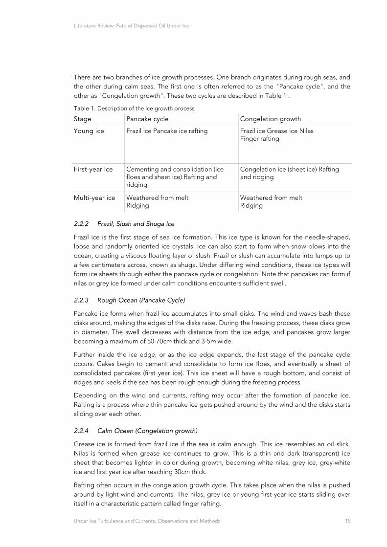
2.2.3 Rough Ocean (Pancake Cycle)
Pancake ice forms when frazil ice accumulates into small disks. The wind and waves bash these disks around, making the edges of the disks raise. During the freezing process, these disks grow in diameter. The swell decreases with distance from the ice edge, and pancakes grow larger becoming a maximum of 50-70cm thick and 3-5m wide.
Further inside the ice edge, or as the ice edge expands, the last stage of the pancake cycle occurs. Cakes begin to cement and consolidate to form ice floes, and eventually a sheet of consolidated pancakes (first year ice). This ice sheet will have a rough bottom, and consist of ridges and keels if the sea has been rough enough during the freezing process.
Depending on the wind and currents, rafting may occur after the formation of pancake ice. Rafting is a process where thin pancake ice gets pushed around by the wind and the disks starts sliding over each other.
2.2.4 Calm Ocean (Congelation growth)
Grease ice is formed from frazil ice if the sea is calm enough. This ice resembles an oil slick. Nilas is formed when grease ice continues to grow. This is a thin and dark (transparent) ice sheet that becomes lighter in color during growth, becoming white nilas, grey ice, grey-white ice and first year ice after reaching 30cm thick.
Rafting often occurs in the congelation growth cycle. This takes place when the nilas is pushed around by light wind and currents. The nilas, grey ice or young first year ice starts sliding over itself in a characteristic pattern called finger rafting.
Literature Review: Fate of Dispersed Oil Under Ice
Under Ice Turbulence and Currents, Observations and Methods 16
As the ice grows thicker, and the ocean is calmed due to the ice barrier, congelation ice forms on the ice base. This ice sheet has a smooth bottom.
2.2.5 Ice Deformation
As mentioned above, both pancakes and sheet ice raft under relatively light winds or ocean currents. After the ice becomes grey-white, over 15cm thickness, pancakes and sheet ice have the possibility to ridge. Ridging occurs if the pancakes or ice sheet are too thick to start rafting under, due to the wind and currents (surface forcing). As the ice becomes thicker, stronger surface forcing is required for ridging to occur. During ridging, the ice bends (fracturing under tensile stress) and piles on top of itself. Lines of ridges will then be formed on the surface. As the ridging occurs, a sail forms from the top of the sea ice while a keel forms underneath. For the ice to be in isostatic balance, the keel is much deeper (approximately 5 times) than the ridge is high. This creates an ice pack with morphology that mechanically stirs the upper ocean, locally increasing turbulence.
2.2.6 Wind Stress Transfer through Ice
The kinetic forcing of the upper ocean is provided by tidal motion and wind stress transfer through the ice-ocean interface. Additionally, because the upper ocean is stratified, ice keels and other roughness elements can transfer momentum from the ice to the ocean through form drag, which generally takes one of two forms: (1) form drag past a blunt object, and (2) generation of internal waves. Form drag is when currents flowing past an ice protuberance generate downstream turbulence, often by flow separation.
This is often realized in sampling by increasing Reynolds stress with depth from the interface. Measurements are usually made under relatively smooth ice, and deeper sampling indicate turbulence generated at a distance from the sampling area. The second mechanism is the generation of internal waves by changing the thickness of the mixed layer overlying a pycnocline. This reduces the overall momentum out of the ice/ IOBL system, hence actually reducing turbulent mixing more than for the first mechanism with the same surface stress. Note that the protuberance does not need to penetrate the pycnocline, but simply occupy a significant fraction of the well mixed layer. Note that if the ice is static and the ocean is in motion, the resulting momentum transfer decelerates the ocean and accelerates the ice. As the ice pack consolidates and forms pack ice, wind stress transfer to the upper ocean is dramatically reduced. At around 95% concentration the ice pack can be considered mechanically connected, such that the ice interaction force is comparable to wind and current stresses, significantly damping wind stress transfer to the ocean. With the onset of climate change, the previous mechanism is seen less in consolidated winter ice in favour of a more free drift state: air stress / Coriolis / water stress with air and water stresses at similar magnitudes, so the wind stress transfer is less reduced.
In looser ice packs, keels and ice bottom roughness allow more effective stress transfer between the wind and ocean. One can expect that loose, highly deformed ice would be effective at transmitting wind stress to the upper ocean as compared to swell, newly formed ice or consolidated pack ice.

Literature Review: Fate of Dispersed Oil Under Ice
Under Ice Turbulence and Currents, Observations and Methods 17
2.2.7 Ice Growth and Melt
Our discussion so far has focussed on the development of sea ice with differing surface roughness that impacts wind stress transfer to the upper ocean. Other processes that affect upper ocean turbulence in sea ice covered waters are related to the growth and melt of ice.
During ice growth, brine is rejected. As ice is an insulator, young ice grows faster than thicker ice. Hence brine rejection is greater at the onset of freezing, at the ice growing ice edge, in leads and in polynyas. The rejected brine is dense and creates convective overturning in the upper ocean, deepening the mixed layer.
With the onset of ice melt, buoyant fresh water forms the shallow summer mixed layer, increasing upper ocean stratification and reducing turbulent mixing. In considering turbulence in the upper sea ice covered waters one should not decouple mechanical mixing from the buoyancy driven mixing. Hence the importance of considering stage of development (ice type), stage of melt and forcing (tides, winds and internal ice stress) in characterising turbulence under sea ice.
2.2.8 Relevance for Turbulence and Fate of Oil Droplets
During an oil spill in ice covered waters, the oil may be dispersed and trapped under ice floes. The fate of this oil depends on several different factors:
Roughness of the ice bottom.
Under-ice roughness will cause increased oil trapping, and increase turbulence.
Oil will move more freely beneath a smooth ice bottom, and friction is reduced.
Sea ice with a smooth underside will drift more rapidly than very rough or ridged pack ice
Depth of ice keels (i.e. very rough ice) will affect the Ekman veering angle relative to the wind direction, and the relative motion of the ice relative to a cloud of droplets underneath.
Size of the ice floe/cover/sheet, or concentration and consolidation of the ice pack.
A more consolidated ice pack reduces wind stress transfer to the upper ocean, reducing turbulence.
Ice cover concentration.
Damping of waves will reduces vertical turbulence, so degree of ice cover as well as distance from the ice edge will be significant parameters in the problem.
Strength of the under ice current.
Stronger currents relative to the ice will produce higher turbulence levels for a given mean roughness measure.
Freezing and melting processes.
Freezing processes may cause oil to be frozen into the ice floe and thus be transported with the drift of the ice, to be eventually released again during breakup.
Literature Review: Fate of Dispersed Oil Under Ice
Under Ice Turbulence and Currents, Observations and Methods 18
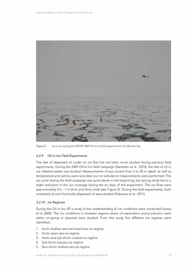
Figure 2. Ice cover during the SINTEF 2009 Oil-In-Ice field experiment in the Barents Sea.
2.2.9 Oil-in-Ice Field Experiments
The fate of dispersed oil under an ice floe has not been much studied during previous field experiments. During the 2009 Oil-In-Ice field campaign (Sørstrøm et al., 2010), the fate of oil in ice infested waters was studied. Measurements of sea current from 5 to 30 m depth as well as temperature and salinity were recorded, but no turbulence measurements were performed. The ice cover during the field campaign was quite dense in the beginning, but strong winds led to a slight reduction in the ice coverage during the six days of the experiment. The ice floes were approximately 0.5 - 1 m thick and fairly small (see Figure 2). During the field experiments, both untreated oil and chemically dispersed oil were studied (Faksness et al., 2011).
2.2.10 Ice Regimes
During the Oil in Ice JIP a study of the understanding of ice conditions were conducted (Lewis et al.,2008). The ice conditions in nineteen regions where oil exploration and production were either on-going or planned were studied. From this study five different ice regimes were identified:
1. Arctic shallow semi-enclosed sea ice regime 2. Arctic open sea ice regime 3. Arctic and sub-Arctic coastal ice regime 4. Sub-Arctic estuary ice regime 5. Non-Arctic shallow sea ice regime

Literature Review: Fate of Dispersed Oil Under Ice
Under Ice Turbulence and Currents, Observations and Methods 19
For each of these sea ice regimes, the following ice characteristics were described:
Concentration
Age
Thickness
Type/size
Movement
The identification of these five ice regimes and the description of the ice characteristics will help us in the decision on areas that are best suited for field measurements.
Under Ice Turbulence Measurement Techniques 2.3
Here we review methods for measuring turbulence in the sea-ice environment and IOBL. We will begin with the methods most suitable to measuring turbulence in the IOBL, but also mention other methods of potential relevance. Older instrumentation not generally in usage today, such as rotor current meters or hot-film anemometers, is not considered.
2.3.1 Turbulence Instrument Clusters (TICs)
In the polar oceans a major motivation for turbulence research has been to quantify turbulent exchanges (Reynold’s fluxes) between the air-ice-ocean systems and to understand the role of these exchanges in controlling the growth and loss of sea-ice cover. The stable platform of the ice makes direct measurement of the under-ice fluctuations of velocity, temperature and salinity viable. Practically speaking this has meant that the best modern measurement approaches in the IOBL are combinations of high frequency acoustic Doppler velocimeters (ADVs). ADVs make measurements in a very small volume, in concert with fast response measurements of temperature (T) and conductivity (C). McPhee refers to arrangements of ADVs with Sea-Bird T and C sensors mounted nearby in the same horizontal plane as turbulence instrument clusters (TICs) and they are typically arranged on rigid masts that are either suspended directly from the ice, or on a flexible cable allowing the mast to be situated at various depths. TIC masts can extend through the under-ice boundary layer and directly measure turbulent Reynold’s stress, ⟨ ′ ′⟩, heat flux, ⟨ ′ ′⟩, and salinity flux, . In concert with
measurements of mean currents and stratification using Doppler current profilers (ADCPs – discussed below), and scalar fluxes are directly related to the shear and buoyancy production
terms of the turbulent kinetic energy equation. The assumptions moving from covariances averaged over tens of minutes to turbulent fluxes are (i) the flow is suitably steady compared with changes in the mean flow (i.e., that a "spectral gap" exists) and (ii) the flow is horizontally homogeneous enough to apply Taylor's hypothesis relating time series covariance with ensemble average of the deviatory products.
TICs are designed to measure the fluxes associated with turbulent covariances. In order to measure turbulent dissipation rate in the near-ice boundary layer, the turbulent dissipation rate, ∈, has been estimated using the inertial dissipation method (IDM). The spectrum of kinetic energy in the inertial subrange, i.e. the intermediate scales between the larger energy containing eddies and scales where turbulence removes energy from the flow through molecular viscosity, is frequently found to have a spectral shape
∈ ⁄ ⁄ (1)
Literature Review: Fate of Dispersed Oil Under Ice
Under Ice Turbulence and Currents, Observations and Methods 20
based on dimensional arguments by Kolmogorov. is a dimensionless constant frequentlytaken to be 1.5 (Tennekes; Lumley 1972a). Measurement of a single component of velocity is easier, so the corresponding spectrum of kinetic energy from a single velocity component is
Φ ∈ ⁄ ⁄ (2)
And is taken to be 0.5.
In the IDM approach, currents are measured at a single location and time-domain fluctuations (frequency spectra, ) are converted to wavenumber spectra, , through Taylor’s “frozen field” hypothesis through the relationship / , where is the low-frequency/wavenumber background flow. In this manner point measurements of flow are used to estimate . McPhee (1998b) extended the IDM method to estimate turbulent fluxes of scalars such as salt heat or buoyancy in convective boundary layers.
2.3.2 Shear Microstructure
Shear microstructure allows for the direct computation of TKE dissipation, (Lueck et al. 2002; Thorpe 2007). Early measurements of ocean turbulence were based on hot-film anemometers and cold film thermometers placed on the bow of ships or towed bodies (Grant et al. 1962; Lueck et al. 2002) that sample turbulence horizontally. These techniques were effective in coastal tidal environments where turbulence levels are frequently large, but proved more difficult in lower energy environments because of aliasing of the turbulence signals with body motion and the requirement that the flow rate past the sensors be steady. Subsequently, free falling turbulence profilers equipped with fast-response thermistors and shear probes were developed that alleviated many of these problems.
Many of the technical barriers to horizontal sampling of turbulence have since been eliminated and a variety of platforms are now available for mounting instrumentation with turbulence microstructure measurements such as the towed turbulence platform MARLIN (Moum et al. 2002). Although towed bodies offer many advantages, notably their ability to address spatial inhomogeneity, their use is generally impractical in even low concentration ice, because the instrument line snags small pieces which quickly run down toward the instruments. More recently, autonomous underwater vehicle (AUVs) such as the powered AUV REMUS (Goodman et al. 2006; Levine et al. 2009) and SLOCUM gliders (Wolk et al. 2009) have been instrumented with turbulence microstructure instrumentation. Also, progress has been made in operating AUVs under sea ice.
Microstructure instruments measure the component of velocity perpendicular to the motion of the instrument, which is either horizontal or vertical. A microstructure instrument samples velocity fluctuations in time using an airfoil style probe (Lueck et al. 2002). Taylor’s “frozen flow” hypothesis is invoked (Tennekes; Lumley 1972a) which supposes that the probe passes quickly (relative to the evolution of the flow field) through a medium that remains unchanged, and that the turbulence is locally isotropic. Ocean current fluctuations are measured along a profile and the time-domain fluctuations (frequency spectra, ) are converted to wavenumber spectra, , through the relationship ⁄ ,where is the mean speed of the instrument through the water.
Under the assumption that this turbulence is isotropic, we then write
Literature Review: Fate of Dispersed Oil Under Ice
Under Ice Turbulence and Currents, Observations and Methods 21
Φ (3)
Where is the viscosity of sea water and are the turbulent velocity fluctuations perpendicular to the motion of the instrument.
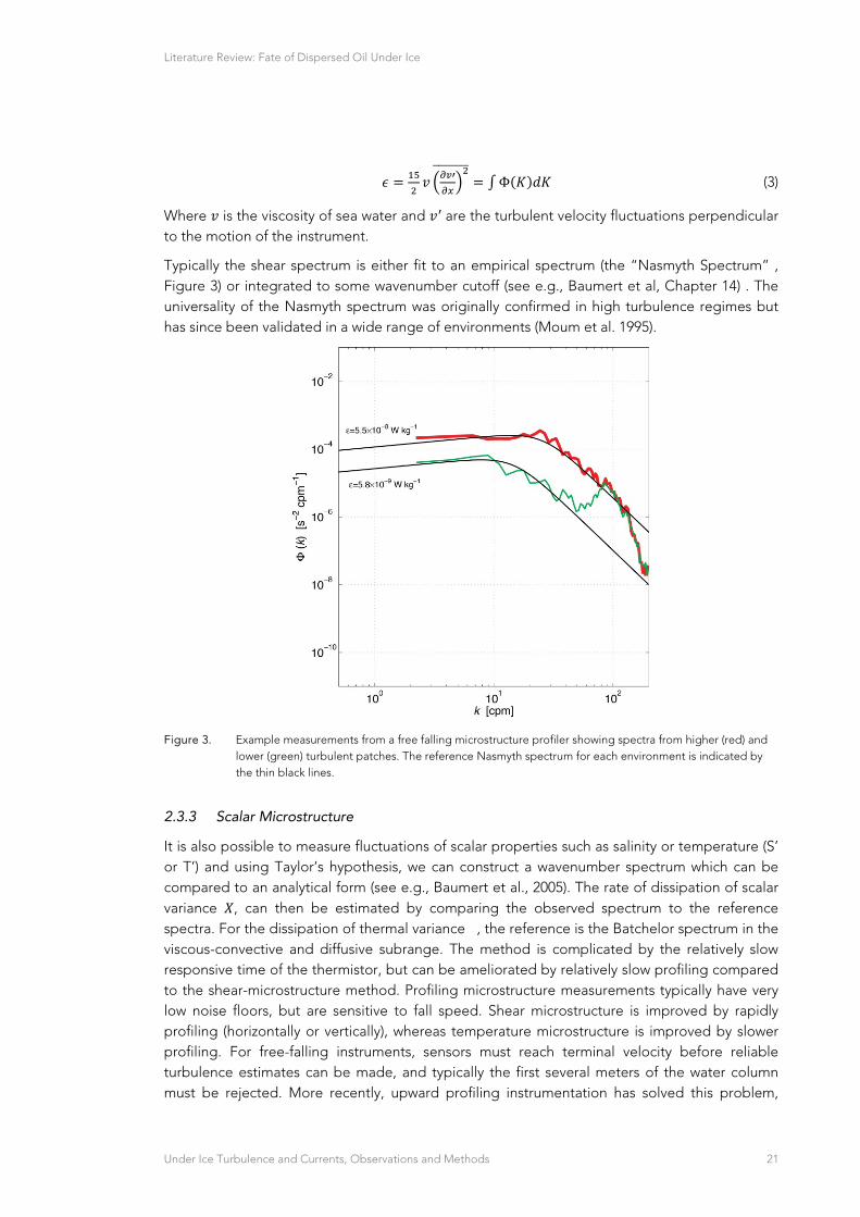
Typically the shear spectrum is either fit to an empirical spectrum (the “Nasmyth Spectrum” , Figure 3) or integrated to some wavenumber cutoff (see e.g., Baumert et al, Chapter 14) . The universality of the Nasmyth spectrum was originally confirmed in high turbulence regimes but has since been validated in a wide range of environments (Moum et al. 1995).
Figure 3. Example measurements from a free falling microstructure profiler showing spectra from higher (red) and lower (green) turbulent patches. The reference Nasmyth spectrum for each environment is indicated by the thin black lines.
2.3.3 Scalar Microstructure
It is also possible to measure fluctuations of scalar properties such as salinity or temperature (S’ or T’) and using Taylor’s hypothesis, we can construct a wavenumber spectrum which can be compared to an analytical form (see e.g., Baumert et al., 2005). The rate of dissipation of scalar variance , can then be estimated by comparing the observed spectrum to the reference spectra. For the dissipation of thermal variance , the reference is the Batchelor spectrum in the viscous-convective and diffusive subrange. The method is complicated by the relatively slow responsive time of the thermistor, but can be ameliorated by relatively slow profiling compared to the shear-microstructure method. Profiling microstructure measurements typically have very low noise floors, but are sensitive to fall speed. Shear microstructure is improved by rapidly profiling (horizontally or vertically), whereas temperature microstructure is improved by slower profiling. For free-falling instruments, sensors must reach terminal velocity before reliable turbulence estimates can be made, and typically the first several meters of the water column must be rejected. More recently, upward profiling instrumentation has solved this problem,
Literature Review: Fate of Dispersed Oil Under Ice
Under Ice Turbulence and Currents, Observations and Methods 22
allowing measurements into the upper meter of the water column. In broken ice, this could prove risky to the instrumentation.
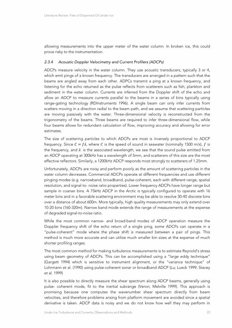
2.3.4 Acoustic Doppler Velocimetry and Current Profilers (ADCPs)
ADCPs measure velocity in the water column. They use acoustic transducers, typically 3 or 4, which emit pings of a known frequency. The transducers are arranged in a pattern such that the beams are angled away from each other. ADPCs transmit a ping at a known frequency, and listening for the echo returned as the pulse reflects from scatterers such as fish, plankton and sediment in the water column. Currents are inferred from the Doppler shift of the echo and allow an ADCP to measure currents parallel to the beams in a series of bins typically using range-gating technology (RDInstruments 1996). A single beam can only infer currents from scatters moving in a direction radial to the beam path, and we assume that scattering particles are moving passively with the water. Three-dimensional velocity is reconstructed from the trigonometry of the beams. Three beams are required to infer three-dimensional flow, while four beams allows for redundant calculation of flow, improving accuracy and allowing for error estimates.
The size of scattering particles to which ADCPs are most is inversely proportional to ADCP frequency. Since , where is the speed of sound in seawater (nominally 1500 m/s), is the frequency, and is the associated wavelength, we see that the sound pulse emitted from an ADCP operating at 300kHz has a wavelength of 5mm, and scatterers of this size are the most effective reflectors. Similarly, a 1200kHz ADCP responds most strongly to scatterers of 1.25mm.
Unfortunately, ADCPs are noisy and perform poorly as the amount of scattering particles in the water column decreases. Commercial ADCPs operate at different frequencies and use different pinging modes (e.g. narrowband, broadband, pulse-coherent, each with different range, spatial resolution, and signal-to- noise ratio properties). Lower frequency ADCPs have longer range but sample in coarser bins. A 75kHz ADCP in the Arctic is typically configured to operate with 16 meter bins and in a favorable scattering environment may be able to resolve 30-40 discrete bins over a distance of about 600m. More typically, high quality measurements may only extend over 10-20 bins (160-320m). Narrow band mode extends the range of measurements at the expense of degraded signal-to-noise ratio.
While the most common narrow- and broad-band modes of ADCP operation measure the Doppler frequency shift of the echo return of a single ping, some ADCPs can operate in a “pulse-coherent” mode where the phase shift is measured between a pair of pings. This method is much more accurate and can utilize much smaller bin sizes at the expense of much shorter profiling ranges.
The most common method for making turbulence measurements is to estimate Reynold’s stress using beam geometry of ADCPs. This can be accomplished using a “large eddy technique” (Gargett 1994) which is sensitive to instrument alignment, or the “variance technique” of Lohrmann et al. (1990) using pulse-coherent sonar or broadband ADCP (Lu; Lueck 1999; Stacey et al. 1999)
It is also possible to directly measure the shear spectrum along ADCP beams, generally using pulse- coherent mode, fit to the inertial subrange (Veron; Melville 1999). This approach is promising because one computes the wavenumber shear spectrum directly from beam velocities, and therefore problems arising from platform movement are avoided since a spatial derivative is taken. ADCP data is noisy and we do not know how well they may perform in
Literature Review: Fate of Dispersed Oil Under Ice
Under Ice Turbulence and Currents, Observations and Methods 23
extremely low energy environments as may be encountered under sea ice. In the MIZ, this type of measurement may be contaminated by a lack of a spectral gap between orbital wave motions and turbulence. Pulse coherent mode measurements are more accurate than both broadband or narrowband measurements, and may justify this approach.
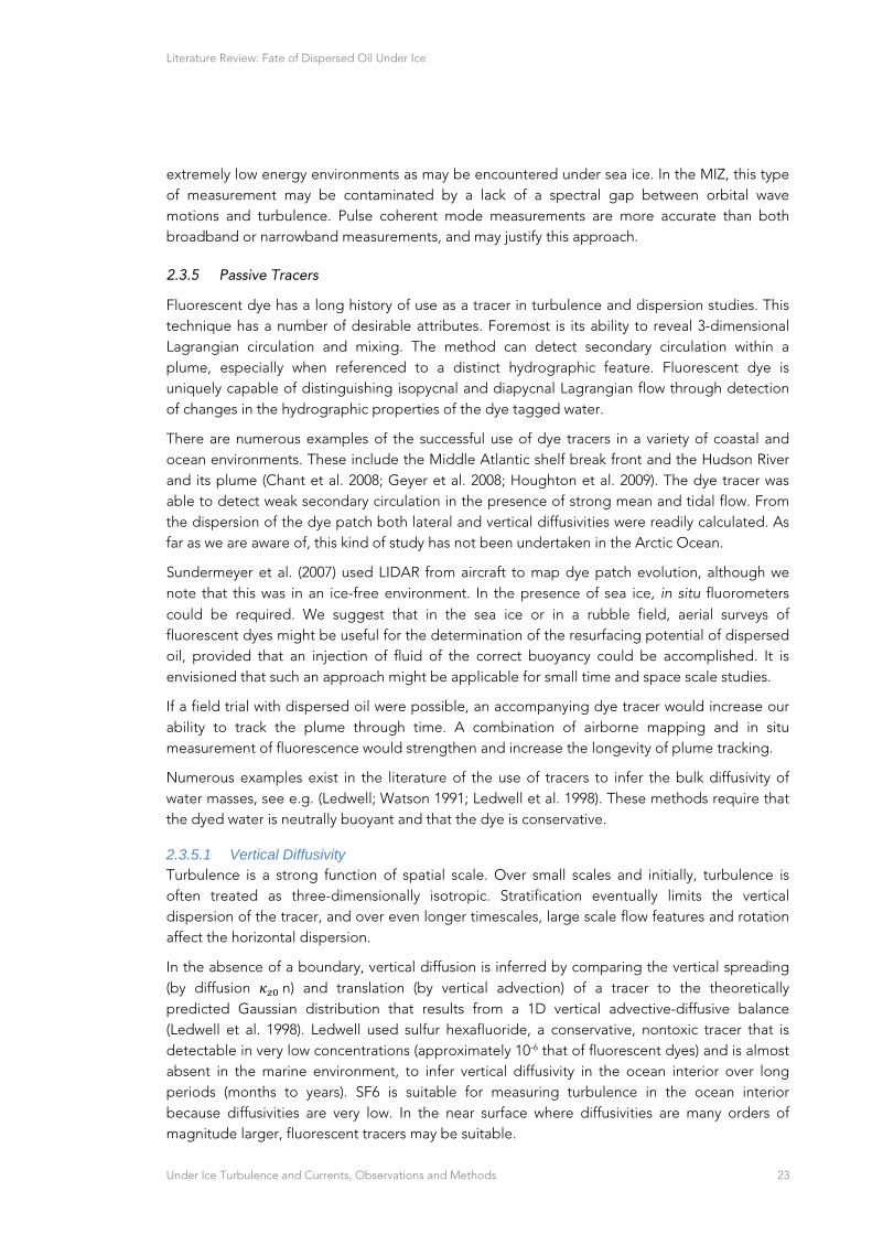
2.3.5 Passive Tracers
Fluorescent dye has a long history of use as a tracer in turbulence and dispersion studies. This technique has a number of desirable attributes. Foremost is its ability to reveal 3-dimensional Lagrangian circulation and mixing. The method can detect secondary circulation within a plume, especially when referenced to a distinct hydrographic feature. Fluorescent dye is uniquely capable of distinguishing isopycnal and diapycnal Lagrangian flow through detection of changes in the hydrographic properties of the dye tagged water.
There are numerous examples of the successful use of dye tracers in a variety of coastal and ocean environments. These include the Middle Atlantic shelf break front and the Hudson River and its plume (Chant et al. 2008; Geyer et al. 2008; Houghton et al. 2009). The dye tracer was able to detect weak secondary circulation in the presence of strong mean and tidal flow. From the dispersion of the dye patch both lateral and vertical diffusivities were readily calculated. As far as we are aware of, this kind of study has not been undertaken in the Arctic Ocean.
Sundermeyer et al. (2007) used LIDAR from aircraft to map dye patch evolution, although we note that this was in an ice-free environment. In the presence of sea ice, in situ fluorometers could be required. We suggest that in the sea ice or in a rubble field, aerial surveys of fluorescent dyes might be useful for the determination of the resurfacing potential of dispersed oil, provided that an injection of fluid of the correct buoyancy could be accomplished. It is envisioned that such an approach might be applicable for small time and space scale studies.
If a field trial with dispersed oil were possible, an accompanying dye tracer would increase our ability to track the plume through time. A combination of airborne mapping and in situ measurement of fluorescence would strengthen and increase the longevity of plume tracking.
Numerous examples exist in the literature of the use of tracers to infer the bulk diffusivity of water masses, see e.g. (Ledwell; Watson 1991; Ledwell et al. 1998). These methods require that the dyed water is neutrally buoyant and that the dye is conservative.
2.3.5.1 Vertical Diffusivity Turbulence is a strong function of spatial scale. Over small scales and initially, turbulence is often treated as three-dimensionally isotropic. Stratification eventually limits the vertical dispersion of the tracer, and over even longer timescales, large scale flow features and rotation affect the horizontal dispersion.
In the absence of a boundary, vertical diffusion is inferred by comparing the vertical spreading (by diffusion n) and translation (by vertical advection) of a tracer to the theoretically predicted Gaussian distribution that results from a 1D vertical advective-diffusive balance (Ledwell et al. 1998). Ledwell used sulfur hexafluoride, a conservative, nontoxic tracer that is detectable in very low concentrations (approximately 10-6 that of fluorescent dyes) and is almost absent in the marine environment, to infer vertical diffusivity in the ocean interior over long periods (months to years). SF6 is suitable for measuring turbulence in the ocean interior because diffusivities are very low. In the near surface where diffusivities are many orders of magnitude larger, fluorescent tracers may be suitable.
Literature Review: Fate of Dispersed Oil Under Ice
Under Ice Turbulence and Currents, Observations and Methods 24
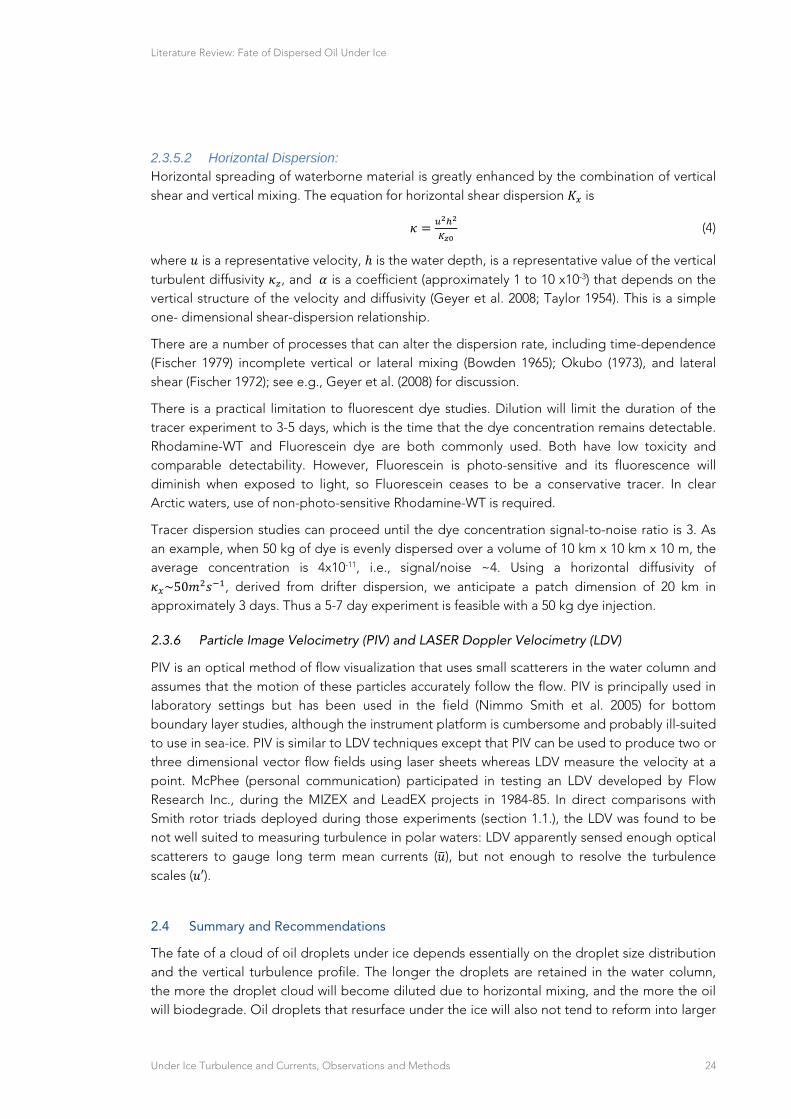
2.3.5.2 Horizontal Dispersion: Horizontal spreading of waterborne material is greatly enhanced by the combination of vertical shear and vertical mixing. The equation for horizontal shear dispersion is
(4)
where is a representative velocity, is the water depth, is a representative value of the vertical turbulent diffusivity , and is a coefficient (approximately 1 to 10 x10-3) that depends on the vertical structure of the velocity and diffusivity (Geyer et al. 2008; Taylor 1954). This is a simple one- dimensional shear-dispersion relationship.
There are a number of processes that can alter the dispersion rate, including time-dependence (Fischer 1979) incomplete vertical or lateral mixing (Bowden 1965); Okubo (1973), and lateral shear (Fischer 1972); see e.g., Geyer et al. (2008) for discussion.
There is a practical limitation to fluorescent dye studies. Dilution will limit the duration of the tracer experiment to 3-5 days, which is the time that the dye concentration remains detectable. Rhodamine-WT and Fluorescein dye are both commonly used. Both have low toxicity and comparable detectability. However, Fluorescein is photo-sensitive and its fluorescence will diminish when exposed to light, so Fluorescein ceases to be a conservative tracer. In clear Arctic waters, use of non-photo-sensitive Rhodamine-WT is required.
Tracer dispersion studies can proceed until the dye concentration signal-to-noise ratio is 3. As an example, when 50 kg of dye is evenly dispersed over a volume of 10 km x 10 km x 10 m, the average concentration is 4x10-11, i.e., signal/noise ~4. Using a horizontal diffusivity of ~50 , derived from drifter dispersion, we anticipate a patch dimension of 20 km in
approximately 3 days. Thus a 5-7 day experiment is feasible with a 50 kg dye injection.
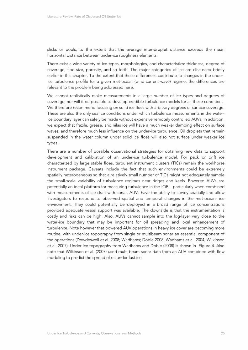
2.3.6 Particle Image Velocimetry (PIV) and LASER Doppler Velocimetry (LDV)
PIV is an optical method of flow visualization that uses small scatterers in the water column and assumes that the motion of these particles accurately follow the flow. PIV is principally used in laboratory settings but has been used in the field (Nimmo Smith et al. 2005) for bottom boundary layer studies, although the instrument platform is cumbersome and probably ill-suited to use in sea-ice. PIV is similar to LDV techniques except that PIV can be used to produce two or three dimensional vector flow fields using laser sheets whereas LDV measure the velocity at a point. McPhee (personal communication) participated in testing an LDV developed by Flow Research Inc., during the MIZEX and LeadEX projects in 1984-85. In direct comparisons with Smith rotor triads deployed during those experiments (section 1.1.), the LDV was found to be not well suited to measuring turbulence in polar waters: LDV apparently sensed enough optical scatterers to gauge long term mean currents ( ), but not enough to resolve the turbulence scales ( ′).
Summary and Recommendations 2.4
The fate of a cloud of oil droplets under ice depends essentially on the droplet size distribution and the vertical turbulence profile. The longer the droplets are retained in the water column, the more the droplet cloud will become diluted due to horizontal mixing, and the more the oil will biodegrade. Oil droplets that resurface under the ice will also not tend to reform into larger
Literature Review: Fate of Dispersed Oil Under Ice
Under Ice Turbulence and Currents, Observations and Methods 25
slicks or pools, to the extent that the average inter-droplet distance exceeds the mean horizontal distance between under-ice roughness elements.
There exist a wide variety of ice types, morphologies, and characteristics: thickness, degree of coverage, floe size, porosity, and so forth. The major categories of ice are discussed briefly earlier in this chapter. To the extent that these differences contribute to changes in the under-ice turbulence profile for a given met-ocean (wind-current-wave) regime, the differences are relevant to the problem being addressed here.
We cannot realistically make measurements in a large number of ice types and degrees of coverage, nor will it be possible to develop credible turbulence models for all these conditions. We therefore recommend focusing on solid ice floes with arbitrary degrees of surface coverage. These are also the only sea ice conditions under which turbulence measurements in the water-ice boundary layer can safely be made without expensive remotely controlled AUVs. In addition, we expect that frazile, grease, and nilas ice will have a much weaker damping effect on surface waves, and therefore much less influence on the under-ice turbulence. Oil droplets that remain suspended in the water column under solid ice floes will also not surface under weaker ice types.
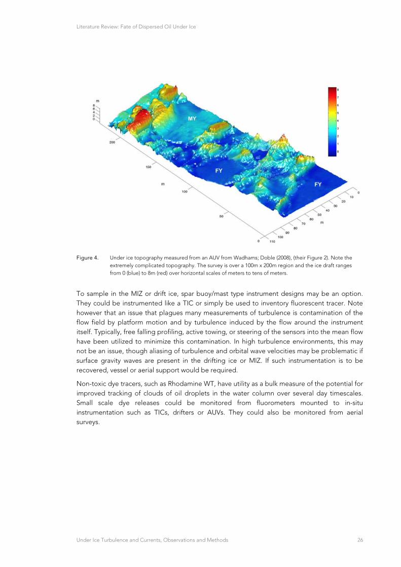
There are a number of possible observational strategies for obtaining new data to support development and calibration of an under-ice turbulence model. For pack or drift ice characterized by large stable floes, turbulent instrument clusters (TICs) remain the workhorse instrument package. Caveats include the fact that such environments could be extremely spatially heterogeneous so that a relatively small number of TICs might not adequately sample the small-scale variability of turbulence regimes near ridges and keels. Powered AUVs are potentially an ideal platform for measuring turbulence in the IOBL, particularly when combined with measurements of ice draft with sonar. AUVs have the ability to survey spatially and allow investigators to respond to observed spatial and temporal changes in the met-ocean- ice environment. They could potentially be deployed in a broad range of ice concentrations provided adequate vessel support was available. The downside is that the instrumentation is costly and risks can be high. Also, AUVs cannot sample into the log-layer very close to the water-ice boundary that may be important for oil spreading and local enhancement of turbulence. Note however that powered AUV operations in heavy ice cover are becoming more routine, with under-ice topography from single or multibeam sonar an essential component of the operations (Dowdeswell et al. 2008; Wadhams; Doble 2008; Wadhams et al. 2004; Wilkinson et al. 2007). Under ice topography from Wadhams and Doble (2008) is shown in Figure 4. Also note that Wilkinson et al. (2007) used multi-beam sonar data from an AUV combined with flow modeling to predict the spread of oil under fast ice.
Literature Review: Fate of Dispersed Oil Under Ice
Under Ice Turbulence and Currents, Observations and Methods 26
Figure 4. Under ice topography measured from an AUV from Wadhams; Doble (2008), (their Figure 2). Note the extremely complicated topography. The survey is over a 100m x 200m region and the ice draft ranges from 0 (blue) to 8m (red) over horizontal scales of meters to tens of meters.
To sample in the MIZ or drift ice, spar buoy/mast type instrument designs may be an option. They could be instrumented like a TIC or simply be used to inventory fluorescent tracer. Note however that an issue that plagues many measurements of turbulence is contamination of the flow field by platform motion and by turbulence induced by the flow around the instrument itself. Typically, free falling profiling, active towing, or steering of the sensors into the mean flow have been utilized to minimize this contamination. In high turbulence environments, this may not be an issue, though aliasing of turbulence and orbital wave velocities may be problematic if surface gravity waves are present in the drifting ice or MIZ. If such instrumentation is to be recovered, vessel or aerial support would be required.
Non-toxic dye tracers, such as Rhodamine WT, have utility as a bulk measure of the potential for improved tracking of clouds of oil droplets in the water column over several day timescales. Small scale dye releases could be monitored from fluorometers mounted to in-situ instrumentation such as TICs, drifters or AUVs. They could also be monitored from aerial surveys.
Literature Review: Fate of Dispersed Oil Under Ice
Models 27
CHAPTER 3. MODELS
Turbulent Transport Modeling in the Ice-Ocean Boundary Layer 3.1
Scalar contaminants in the water column, including dispersed oil droplets, interact with sea ice via turbulent exchange through an ice-ocean boundary layer (IOBL). While in general all planetary boundary layers share similar equations, the IOBL differs from the open ocean surface boundary layer (OBL) in that sea ice is relatively effective at damping higher frequency surface gravity waves, and presents a more or less solid boundary at the ocean surface. Without the influence of waves and with proper similarity scaling, the IOBL resembles the atmospheric planetary boundary layer, perhaps more than does the OBL, and this has influenced numerical modelling approaches. This section reviews the literature pertaining to IOBL modelling, describes the underlying physical principles, and emphasizes those aspects related to contaminant transfer.
3.1.1 Model Classes, Review of Model Types Applied to the IOBL
Most IOBL modelling efforts fall into one of four categories. In order of increasing complexity they are: (a) slab (mixed layer) models; (b) first-order turbulence closure models; (c) second-moment turbulence closure models, and (d) large-eddy simulation models.
Slab models are adapted from a prototype (Kraus; Turner 1967) in which the OBL is treated as a well- mixed layer with uniform properties (including velocity) overlying a stably stratified pycnocline (density gradient). The momentum and scalar properties of the mixed layer vary in response to surface stress and buoyancy flux (a function of heat and salt fluxes), and by interaction with the underlying thermocline (halocline) if there is an entrainment velocity, , (local time derivative of mixed layer depth). Generally, depends on a combination of the rate of working by stress and buoyancy flux at the surface, usually in the form of bulk Richardson number (Price et al. 1986, PWP). Applications of the bulk PWP approach specifically to the IOBL include recent works by Toole et al. (2010) and (Hyatt 2006).
With proper tuning, the bulk models do well at describing some aspects of air-ocean interaction, but miss important details of variation in the fluxes throughout the so-called well mixed layer. From measurements under sea ice, we know, for example, that there is velocity shear always present in the IOBL (e.g., McPhee; Smith 1976), and that scalar fluxes ( , ) occur only with gradients (albeit small) in the mean quantities (e.g., McPhee; Martinson 1994). Describing turbulent flux of a flow property (momentum, heat, salt) in terms of averaged properties of the flow ( , , ) is the basic turbulence closure problem.
The most commonly accepted methodology for treating turbulence in geophysical flows is by dividing the flow into mean and fluctuating components over a suitable time interval via the Reynolds decomposition (Hinze 1975; Tennekes; Lumley 1972b), then equating the turbulent fluxes to second- moments (covariances) of the quantities with the appropriate velocity component. For example, vertical kinematic turbulent heat flux is the covariance of temperature deviations with vertical velocity. First- order closure refers to expressing the second-moments (flux of a property) directly in terms of the mean gradient of that property. Ekman (1905) expressed turbulent stress as proportional to horizontal velocity shear, with a proportionality constant analogous to molecular viscosity but several orders of magnitude greater in magnitude. His analysis of the IOBL equations led him to what is now known as the Ekman
Literature Review: Fate of Dispersed Oil Under Ice
Models 28
spiral in IOBL velocity structure, and provided qualitative explanation of observations that the drift of the FRAM during Nansen’s 1893-1896 Arctic expedition veered to the right of the surface wind by 20-40 degrees. Fittingly, the best examples of naturally observed Ekman spirals come from measurements in the IOBL from drifting ice stations (e.g., Hunkins (1966);McPhee; Smith (1976)) including a spiral in horizontal turbulent stress predicted by Ekman’s solution (McPhee; Martinson 1994). Ekman considered neither the turbulent transport of scalar properties, nor the related and important impact of buoyancy on eddy viscosity. His depth invariant eddy viscosity also precluded a thin layer of intense shear near the ocean surface, where the velocity profile is logarithmic and eddy viscosity varies linearly with distance from the boundary. Obviously, these deficiencies have been addressed in subsequent 1st-order model developments: one approach called K-profile-parameterization or KPP (Large et al. 1994) has replaced the second-moment schemes described below in some large scale global circulation models, e.g., CCSM3 (Collins et al. 2006). In common with bulk models such as PWP, KPP employs a bulk Richardson number in determining the mixed layer depth. KPP has been “tuned” to large-scale open ocean time series of mixed-layer depth, temperature and salinity, with allowance for horizontal advection. An alternative 1st-order approach based directly on turbulence measurements in the IOBL, called local turbulence closure or LTC (McPhee 2008c) is described in more detail below.
Just as the Reynolds-averaged equations for 1st-moment (mean) quantities include 2nd-moment (variance, covariance) terms, the 2nd-moment equations include 3rd -moment terms, and so on. As computer power increased in the 1970s, simultaneously solving a set of equations carrying the 2nd-moment terms explicitly became possible, closing the system by expressing the 3rd-order terms as functions of lower- order terms (Wyngaard 1975; Wyngaard et al. 1974). The true 2nd-order solution involved a set of 14 simultaneous equations, making calculations cumbersome for application to geophysical problems, leading Mellor; Yamada (1982) to develop a hierarchy of increasingly simplified equation systems. Their model version labelled “2½” (MY2.5) satisfied criteria they deemed suitable for addressing most planetary boundary layer situations, and is used for both atmospheric and oceanic modelling. MY2.5 solves a system of six time-dependent, simultaneous equations: two horizontal velocity components, two scalar equations (T/S for ocean applications), and conservation equations for TKE (turbulent kinetic energy equation, see below), and a master length scale. Buoyancy enters in the form of “shape functions” that make the eddy viscosity conform to Monin-Obukhov similarity. MY2.5 has been applied in a number of IOBL scenarios (Häkkinen; Mellor 1992; Kantha; Mellor 1989; Mellor; Kantha 1989; Mellor; Häkkinen 1994; Mellor et al. 1986; Steele et al. 1989).
The last model class considered, Large-Eddy Simulation (LES), in essence solves the complete Navier- Stokes equations (not Reynolds averaged) on a grid fine enough in all spatial dimensions to resolve the scales of the large (energy containing) turbulent eddies. First applied to the atmospheric boundary layer by Deardorff (1974), LES was later adapted to the ocean, e.g., by Skyllingstad; Denbo (2001). Given the high spatial resolution required, LES models have not been widely used for regional scale modelling, but have proved useful for very local ocean problems such as simulating flow across a pressure ridge keel (Skyllingstad et al. 2003), development of leads and melt ponds (Skyllingstad; Paulson 2007; Skyllingstad et al. 2005), and for investigating nonlinear equation-of-state effects (cabbelling, thermobaricity) in polar waters (Harcourt 2005).
Literature Review: Fate of Dispersed Oil Under Ice
Models 29
3.1.2 Turbulent Fluxes, TKE, Scales of Turbulence, and First-Order Closure
Turbulent fluxes of momentum and scalar properties are notoriously difficult to measure directly in the surface boundary layer of the open ocean, mainly because the combination of orbital velocities and platform motion resulting from surface gravity waves mask the small deviatory (departure from the mean) velocities and scalar signals necessary for valid covariance statistics. Most turbulence measurements in the open ocean are made with microstructure temperature, conductivity, and shear instruments. Estimates of turbulent kinetic energy (TKE) and scalar dissipation rates are then made from the respective spectra at high wavenumbers (small scales).
By contrast, the wave-dampening platform provided by sea ice has provided an extensive record of direct covariance estimates of turbulent stress and scalar fluxes in the IOBL under a wide variety of forcing conditions, including neutral density stratification (McPhee; Smith 1976; McPhee; Martinson 1994); relatively intense heat flux and melting (McPhee et al. 1987; McPhee et al. 1999; Sirevaag 2009); statically unstable stratification at the edge of a freezing lead (McPhee; Stanton 1996) ; and under ice with hydraulic roughness ranging from hydraulically smooth (Crawford et al. 1999; McPhee et al. 2008) to several centimeters (Shaw et al. 2008) (a range of four orders of magnitude). In addition to mean quantities ( , , ), these measurements have included the vertical components of kinematic turbulent stress, ⟨ ′ ′⟩ ⟨ ′ ′⟩; turbulent heat flux, ⟨ ′ ′⟩ where is water density and is specific
heat at constant pressure; salinity flux, ⟨ ′ ′⟩ twice the TKE per unit mass, ⟨ ′ ′⟩ ⟨ ′ ′⟩⟨ ′ ′⟩; as well as variance spectra of the velocity and scalar components. Here angle brackets indicate deviatory quantities remaining in the Reynolds averaging process, with turbulent flow realizations typically comprising averaging periods of 15 to 60 min in the well mixed IOBL.
The combination of turbulent flux and mean value data at levels throughout the entire IOBL under varying stability conditions, when combined with similarity theory for stratified, planetary boundary layers, provides important guidance for IOBL modelling. Similarity and scaling arguments are presented in detail by McPhee (2008c) and are summarized briefly below.
A unifying concept in turbulence studies is the TKE equation, obtained by forming an energy equation as half the product of the instantaneous equation of motion multiplied by instantaneous velocity, then subtracting the Reynolds averaged form of that equation. The result (see, e.g., Hinze (1975)) is quite complex, but when simplified substantially by assuming steady flow and horizontal homogeneity, results in a balance among four terms:
(5)
where ∙ ⁄ is the production rate of TKE by shear (stress multiplied by shear);⟨ ⟩ ⟨ ′⟩⁄ is the TKE production rate by buoyancy; is the divergence of a
combination of vertical flux of TKE and of the covariance of vertical velocity with pressure fluctuations; and is the dissipation of TKE at molecular scales. The divergence term, , is difficult to measure directly and researchers have often assumed that its two constituents are small or effectively cancel. TKE dissipation, , represents conversion of TKE to heat and occurs
via molecular viscosity ( ), at the Kolmogorov length and velocity scales: / / and ⁄ , respectively. Typical Kolmogorov length and velocity scales for turbulence in the
IOBL are ~2 and ~1 .
The Kolmogorov hypothesis (that at small enough scales, turbulence is statistically in equilibrium and uniquely determined by and (e.g., Hinze 1975)) underscores the relationship between TKE and turbulence at small scales. At the opposite end of the
Literature Review: Fate of Dispersed Oil Under Ice
Models 30
wavenumber spectrum of turbulence, where production of TKE from instabilities in the large-scale flow occurs, IOBL turbulence studies have provided an important empirical basis for defining the important velocity and length scales.
Ekman’s basic idea that turbulent exchange can be closed at first order by relating kinematic stress to velocity shear requires an eddy viscosity, . In order to satisfy dimensional constraints,
, where and are velocity and length scales characterizing turbulent exchanges by the largest (energy containing) eddies. Based on a combination of dimensional analysis (Barenblatt 1996), similarity theory for the stably stratified boundary layer (McPhee 1981), empirical evidence from IOBL measurements, and consideration of the TKE equation, the following scales emerge (McPhee 2008c, Chap. 5). For velocity, define friction speed as the
square root of local kinematic stress: ∗ √ , then
∗
∗ ⟨ ⟩ ⁄
(6)
where the second scale, ∗ , approaches ∗ for weak stratification (shear dominant) but allows for turbulence from convection without mean shear, in which case is some fraction (typically 0.2 to 0.4) of the mixed layer depth.
IOBL research indicates that four turbulence length scales characterize IOBL turbulence under differing conditions of stress, buoyancy, and location relative to the boundary. They are
(i) the distance from the boundary; (ii) the planetary scale, ∗/ where is the Coriolis parameter; (iii) the Obukhov scale; and (iv) in the case of statically unstable convection, the depth of the mixed layer.
In general, the smallest scale exerts most control. A realistic first-order closure model, LTC, for vertical fluxes in terms of mean vertical velocity and scalar profiles follows from proper choices for these scales (McPhee 1994a, 1999, 2008c).
Near the surface in the neutrally buoyant atmospheric boundary layer, extensive measurements have established that the wind profile is logarithmic, thus the turbulence scale (mixing length) is
. At some greater distance, however, rotation becomes important and the planetary scale dominates. Since atmospheric and ocean boundary stress is approximately equal (at least for thin ice) the planetary scales in the atmosphere and ocean will differ by a factor of
⁄ 30, the counterpart of a 1-km thick atmospheric boundary layer would extend about 30 m in the ocean. This rule-of-thumb suggests that if the logarithmic layer extends 60-100 m in the atmosphere, then this layer will extend only 2-3 m from the ice-ocean interface. Beyond that distance, no longer depends on .
Measurements through the outer IOBL have provided strong evidence that beyond the first few meters from the boundary, the neutral mixing length is indeed proportional to some small fraction of the planetary scale: Λ∗ ∗⁄ with Λ∗ 0.03 (McPhee 1994a, 2008b; McPhee; Martinson 1994). The main challenge for 1st-order closure is thus treatment of buoyancy flux. The LTC approach follows from consideration of the simplified TKE (Equation 5) non-dimensionalized by , under the assumption that is negligible and that stress and shear are related by ⁄ / ∗/ :
For neutral or stable stratification
For statically unstable stratification ∗
Literature Review: Fate of Dispersed Oil Under Ice
Models 31
1 1 1⟨ ⟩
∗1
∗ (7)
The progression of equalities in (7) encapsulates a great deal of what is known about the impact of buoyancy on turbulence. The ratio of buoyancy production to shear production is the flux Richardson number, . Positive subtracts TKE because turbulence must work against gravity.
Observations indicate that turbulence no longer persists if exceeds a critical value, , i.e.,
for viable turbulence, 0.2 (Tennekes; Lumley 1972b). The 3rd and 4th terms in (7)
illustrate that / , which is the ratio of mixing length to the Obukhov length,
∗ ⟨ ⟩⁄ (Obukhov 1971).
Note that when buoyancy flux is small, is larger than other scales in the flow, and thus has little impact on turbulence. Conversely, as buoyancy flux increases, becomes dominant, and indeed since must be less than for turbulence to exist, (7) constrains the maximum
turbulent length scale in the flow: . The asymptotic neutral and stratified limits for maximum mixing length in a stratified flow ( positive) are thus
→ Λ∗ ∗⁄ ; for → ∞
→ ; for → 0 (8)
These limits govern scales for the analytic similarity theory of the planetary boundary layer stabilized by surface buoyancy flux developed by McPhee (1981), which specifies the maximum mixing length in the IOBL stabilized by melting as
→ Λ∗ ∗⁄ ; for → ∞
η∗ 1 ∗ ∗⁄
1 ∗ ∗⁄ (9)
In Equation 9, the stability parameter ∗ combines three “universal” parameters ( , , Λ∗) with the ratio of the planetary scale to the Obukhov length, ∗. For ice melting at a rate of 10 cm per day and typical ice pack stress, ∗~0.5 which reduces the effective range of IOBL turbulent mixing by about half. The LTC model utilizes the similarity scaling of Equation (9) to specify mixing length in different regions of the IOBL according to the schematic of Figure 5, then solves the conservation equations for momentum, heat, and salt via an implicit algorithm. Several examples of the time-dependent, horizontally homogeneous solutions of the LTC model, including diurnal heating of the mixed layer at the SHEBA station; the impact of inertial oscillation on mixing at the pycnocline interface during SHEBA; and the development of uniform property layers below the IOBL resulting from nonlinear equation-of-state instabilities are given by McPhee (2008c, Chap. 8).
In addition to LTC's basis in actual measurements, a distinct advantage of LTC over 2nd –moment closure models is that LTC can be used in a “steady” variant, in which isolated samples in time and space (e.g., from a single station with surface stress and buoyancy flux estimates) can be used to produce profile estimates of fluxes in the lower part of the IOBL. Using this approach, a time-dependent model that carried conservation equations only for and was shown to agree closely with a MY2.5 (six conservation equations) when forced with identical surface conditions (McPhee 1999). The approach has also been used to estimate area averages of basal hydraulic roughness (McPhee 2008b; Shaw et al. 2008; Sirevaag et al. 2010).

Literature Review: Fate of Dispersed Oil Under Ice
Models 32
3.1.3 Ocean Drag on Sea Ice: Rossby Similarity
In most dynamic sea-ice models (e.g., Hibler 1979), kinematic basal stress is expressed in terms of ice velocity relative to undisturbed (geostrophic or tidal) flow in the ocean ( ):
∗ ∗ (10)
with constant drag coefficient, , and turning angle, . This is consistent with drag laws applied to measurements in the lower part of the atmospheric boundary layer, but not for stress as a function of geostrophic (pressure gradient) wind, which instead follows a functional form for the neutrally stratified planetary boundary layer analogous to one suggested by Rossby; Montgomery (1935) as modified by Blackadar; Tennekes (1968):
∗⁄ log ∗ (11)
where A and B are constant and f is negative in the southern hemisphere. The dimensionless relative velocity in (11) is the inverse square root of a drag coefficient, which varies in both magnitude and turning angle. In words, Rossby similarity acknowledges the obvious: for the same stress, relatively smooth, first year ice (bottom surface hydraulic roughness, ~ 1 mm) will drift faster than rough, multiyear ice ( ~ 50 mm). A less obvious facet of (11) is that for ice with
specified , the effective drag coefficient ( ∗⁄ / ) decreases with increasing speed, as does the turning angle.
Rossby similarity was extended to the case of rapid melting using the analytic similarity theory based on the scaling of (9) (McPhee 1981) for a modified version of (11):
∗⁄ log ∗∗ ∗ (12)
This relatively simple model for the effective drag coefficient is consistent with atmospheric measurements of geostrophic drag (Clarke; Hess 1974). The analytic solution also provides an expression for near surface dimensionless shear that agrees well with atmospheric measurements (see McPhee (2008c, Fig. 4.9)), particularly under strong inversions over Antarctic ice (Lettau 1979). Its application for modelling sea-ice motion follows from the increase in dimensionless velocity (i.e., reduction in drag) associated with melting. Unless constrained by internal ice forces, ice drifting in above freezing water will move faster and at increased angle to the surface wind than ice would move otherwise. With more open water subject to intense insolation now more prevalent in the Arctic, this tendency for divergence may play an important role in ice-albedo feedback (McPhee 2012).
In the marginal ice zone (MIZ), ice is often subject to conditions not found under a solid ice pack: short period surface waves and relatively warm IOBL temperatures. In the context of contaminant transport within the ice matrix, an important MIZ feature is the production of ice-edge bands that form during off- ice winds and separate rapidly from the main ice pack. Several mechanisms have been advanced for the genesis and motion of ice-edge bands, including (i) enhanced wind drag from wave fracturing (Bauer; Martin 1980; Guest et al. 1995a); (ii) surface gravity wave radiation stress (Martin et al. 1983; Wadhams 1983); (iii) surface manifestation of internal waves in the ocean (Muench et al. 1983); and (iv) reduced ocean drag from rapid melting (McPhee 1981, 1983b; Mellor et al. 1986). In the last mechanism, the band leaves cooler water behind, so that melting is reduced, trailing ice moves slower, and separation
Literature Review: Fate of Dispersed Oil Under Ice
Models 33
results. The similarity approach embodied in (12) provides quantitatively reasonable separation velocities (McPhee 1983b, 2008c). As Weeks (2010) points out, there has been no definitive study that selects one band-formation mechanism over others, and indeed, several may act in concert (e.g., orbital wave velocities enhancing local friction velocity and melt rate), depending on conditions.
3.1.4 Scalar Exchange at the Ice/Ocean Interface: Viscous Sub-Layers
The efficiency with which turbulence can vertically transport salt, heat, or other contaminants depends on both shear induced by stress at the boundary and by buoyancy flux in the fluid. The latter depends critically on rates of freezing or melting at the ice-water interface that govern the boundary buoyancy flux, and has been extensively studied: McPhee et al. (2008) present an overview. Prior to measurements made during the 1984 Marginal Ice Zone Experiment (MIZEX), researchers often assumed that the interface exchange parameters were either independent of the turbulent flow parameters (Josberger 1983) or that the exchanges could be characterized by reduced hydraulic roughness lengths for heat and salt, analogous to atmospheric treatment of heat and water vapour (Mellor et al. 1986). Measurements during the last week of MIZEX, which included for the first time direct ocean turbulent heat flux estimates, ⟨ ′ ′⟩, indicated that the previous exchange rate estimates were far too high, and that unlike momentum, scalar transfer at the interface depended on molecular diffusivities in thin sub-layers adjacent to the interface (McPhee et al. 1987). It was also clear that heat exchange varied with both u* and the elevation of mixed-layer temperature above freezing, Δ . Based on turbulence
measurements made from sea ice under variable conditions of ∗, , and Δ , McPhee (1992b) recommended a simple parameterization for basal heat flux
⟨ ′ ′⟩ ∗ ∗Δ (13)
where ∗ 0.006 is the turbulent Stanton number.
An inconsistency implicit in (13) is that at high melt rates, the actual salinity at the interface may be significantly lower than the far-field (mixed layer) value, and there is considerable evidence (e.g., Notz et al. 2003) that heat is transferred more rapidly than salt at the melting interface, i.e., that melting occurs by a double-diffusive process resulting from the large discrepancy between molecular thermal and haline diffusivities (a factor of about 200). McPhee et al. (2008) describe a framework that accounts for the double-diffusion by combining concepts from laboratory and engineering studies of heat and mass transport over hydraulically rough surfaces (Incropera; DeWitt 1985; Owen; Thomson 1967; Yaglom; Kader 1974), with extensive IOBL turbulence measurements. Turbulent fluxes of heat and salt into an infinitesimal control volume following the interface are expressed as
⟨ ′ ′⟩ ∗
⟨ ′ ′⟩ ∗
Where and are the differences between the far-field and interface values of temperature and salinity, respectively; and and are turbulent exchange factors. Assuming that temperature at the interface is freezing, i.e., that where is the local slope of the freezing curve, and that upward heat conduction in the ice is negligible, conservation equations for and reduce to a quadratic equation for in terms of temperature scales (for a more complete derivation, refer to McPhee (2008c), Chap. 6):
Literature Review: Fate of Dispersed Oil Under Ice
Models 34
0 (14)
where is the apparent latent heat of sea ice (adjusted for brine volume) and / is the ratio of the exchange factors. If molecular diffusivities are important in the problem, theory and observations suggest that ⁄ , where ranges from 2/3 to 0.8, implying 35 70. When 1, heat and salt are transferred at the same rate; for 1 heat is transferred more rapidly so decreases so as to keep
∗ /Δ (15)
in other words, the bulk Stanton number should increase with increasing melt rate. At relatively low melt rates, in the range of most of the under-ice measurements, ∗ constrains but ∗ still depends on . It is notoriously difficult to measure both ⟨ ′ ′⟩ and ⟨ ′ ′⟩ accurately in a rapidly melting environment; however by careful analysis of turbulence measurements in Whaler’s Bay north of Svalbard, Sirevaag (2009) obtained independent estimates of the exchange coefficients: 0.0131 and 4 10 for 33 when the average heat flux was 268 Wm-2. He also reported a bulk Stanton number: ∗ 0.0084, about 5% less than the value predicted by (15) which is 0.0088. His results thus confirm that heat flux increases with thermal driving in a super-linear fashion, with potential importance for estimating ice melt and IOBL stratification in low ice-concentration conditions.
3.1.5 Inertial Oscillations and Internal Waves
Modern navigation methods have shown that cycloidal loops in ice drift trajectories are common, particularly in summer when the ice cover is weak and mixed layers shallow. Away from regions with energetic tides, these are generally manifestations of inertial oscillations in the combined ice/IOBL system forced by relatively abrupt wind shifts. Predicted theoretically by Ekman (1905) (with credit to Fredholm), inertial oscillation in ice motion was first inferred from current measurements in nearly quiescent water below the IOBL (Hunkins 1967; McPhee 1978). When satellite navigation provided accurate position measurement at time scales smaller than the inertial period (12 h at the poles), a technique called complex demodulation was developed to fit observed positions to a function which provided instantaneous velocity and isolated the inertial (and diurnal tidal) components of the drift (McPhee 1988).
Current measurements through the IOBL consistently show that the ice and dominant currents in the IOBL oscillate together inertially (i.e., in phase) and that most of the shear associated with inertial motion occurs in the upper part of the underlying pycnocline. Since the ice and bulk of the IOBL oscillate in phase, shear exhibits little or no inertial component in the upper part of the water column.
This means that drag formulations using to estimate interface turbulent exchange, should be applied only after removing the inertial oscillation component.The importance of inertial oscillation for momentum and scalar fluxes at the base of the IOBL is not thoroughly understood, with different modelling approaches providing very different assessments. Inertial oscillation played a major role in providing the impulse necessary to deepen the mixed layer in some early “slab” models; e.g., in the model of Pollard et al. (1973) all of the deepening occurs in the first half inertial cycle, and any further exchange at the base of the mixed layer happens only if the inertial motion increases in magnitude. On the other hand, based on velocity and turbulence measurements through the entire IOBL, McPhee; Smith (1976) argued that shear persisted throughout the entire boundary layer and that the dynamic boundary layer was not

Literature Review: Fate of Dispersed Oil Under Ice
Models 35
necessarily synonymous with the well mixed layer. From a heuristic viewpoint, inertial oscillations occur because the combined ice/IOBL system lies over a surface (the pycnocline) that is nearly frictionless because turbulence scales are so small. There is, however, evidence that storm events initiate upward and downward propagating near- inertial waves in stratified fluid below the well mixed layer (Merrifield; Pinkel 1996).
By numerical modelling of SHEBA (Surface Heat Budget of the Arctic) IOBL characteristics observed during a period with energetic inertial oscillation in September, 1998, McPhee (2008c, Chap. 8) found little difference in friction velocity and heat flux at both the ice/water interface and at grid points just above the pycnocline, when the model was forced with total surface velocity (including large amplitude inertial waves) versus velocity from which the inertial component had been removed. He concluded that when the underlying pycnocline is strong (as in most of the Arctic), inertial oscillation plays a relatively minor role in IOBL fluxes.
On short time scales (hours to days), prediction of ice motion and IOBL currents depends on proper initialization of the momentum conservation equation. McPhee (2008c, Chap. 8) describes a method for doing this by complex demodulating ice motion (perhaps observed by analysing radar or GPS) for part of an inertial period before the forecast period, then incorporating this into the initial velocity.
Higher frequency internal waves (IWs) may also play a role in IOBL dynamics, but have not received as much attention as other aspects of mixing. Several studies of the deep-ocean IW climate in polar oceans have reported energies consistently below the canonical Garrett-Munk spectrum (Levine et al. 1985; Levine et al. 1997; Plueddemann 1992). The low IW energies below the pycnocline suggest eddy diffusivity magnitudes well below those often invoked for lower latitude oceans, and indeed, shear driven mixing is often thought to be less important than heat flux through double-diffusive step structure (Padman; Dillon 1987; Robertson et al. 1995).
As applied to IOBL modelling, IW research has concentrated on drag generated by the interaction of pressure ridge keels with underlying stratified flow. As reported by Morison (1986), interest in IW drag stems from the “dead water” phenomenon observed when ships lose headway in bays or fjords where brackish water overlies salt water. During the last week of the 1984 MIZEX drift reported above, after the ice had slowed with cessation of the wind, the water column stratified nearly to the ice/water interface. Then as wind increased in the last five days of the project, the effective drag on the underside increased substantially, while the heat transfer coefficient ( ∗) decreased, suggesting that some mechanism besides direct turbulent mixing was active. Morison et al. (1987) ascribed this to pumping momentum flux into the internal wave field, radiating energy away from the IOBL. This left less energy for direct turbulent exchange, thus explaining why scalar exchange factors were reduced relative to momentum. McPhee; Kantha (1989) addressed this quantitatively by deriving the drag associated with a disturbance (pressure ridge keel) advected in an upper ocean comprising a mixed layer separated from an underlying pycnocline by a finite buoyancy jump. From this they calculated a drag coefficient associated with the IW momentum flux, and generalized this drag coefficient to a relatively broad spectrum of underside waviness. By incorporating this into an LTC turbulence closure model, they were able to adequately account for the increased drag and decreased ∗ observed during MIZEX. They concluded that for typical mixed layer depths observed in the Arctic, the IW drag would often be relatively small; however, with the dramatic increase in summer stratification observed in the Canada Basin in recent years, IW drag may well be an important part of the surface momentum balance, and effective scalar exchange factors.
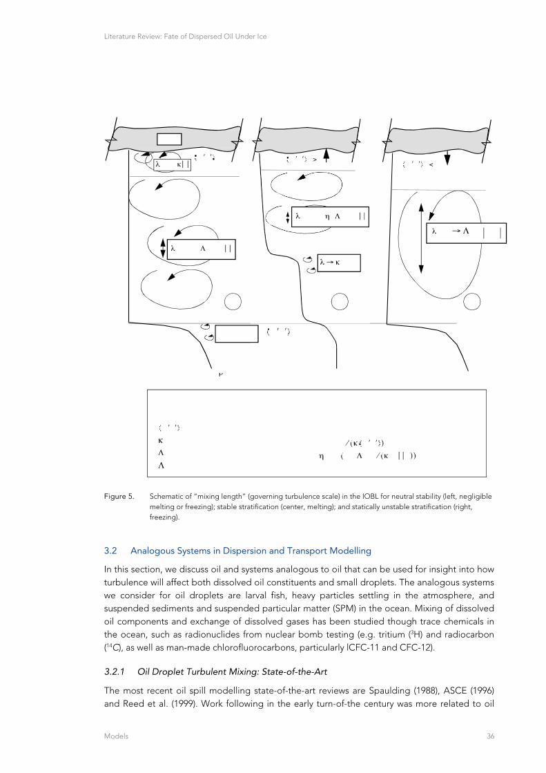
Literature Review: Fate of Dispersed Oil Under Ice
Models 36
Figure 5. Schematic of “mixing length” (governing turbulence scale) in the IOBL for neutral stability (left, negligible melting or freezing); stable stratification (center, melting); and statically unstable stratification (right, freezing).
Analogous Systems in Dispersion and Transport Modelling 3.2
In this section, we discuss oil and systems analogous to oil that can be used for insight into how turbulence will affect both dissolved oil constituents and small droplets. The analogous systems we consider for oil droplets are larval fish, heavy particles settling in the atmosphere, and suspended sediments and suspended particular matter (SPM) in the ocean. Mixing of dissolved oil components and exchange of dissolved gases has been studied though trace chemicals in the ocean, such as radionuclides from nuclear bomb testing (e.g. tritium (3H) and radiocarbon (14C), as well as man-made chlorofluorocarbons, particularly lCFC-11 and CFC-12).
3.2.1 Oil Droplet Turbulent Mixing: State-of-the-Art
The most recent oil spill modelling state-of-the-art reviews are Spaulding (1988), ASCE (1996) and Reed et al. (1999). Work following in the early turn-of-the century was more related to oil

Literature Review: Fate of Dispersed Oil Under Ice
Models 37
dispersion in waves. Tkalich and Chan (2002) developed a model for oil dispersion in breaking waves. Boufadel et al. (2006) did laboratory studies in non-breaking waves, primarily investigating Stokes drift. From Boufadel et al. (2006), the diffusion coefficient depends only on the turbulence intensity. Bechtel et al. (2008) extended this laboratory work to irregular waves. Bandara and Yapa (2011) nicely discuss modelling turbulent collision between bubbles using a method by Prince and Blanch (1990), which should be considered in implementation of the turbulence model.
The laboratory work of Gopalan and Katz (2008) looked at turbulent diffusion of slightly buoyant oil droplets in isotropic turbulence, and the chemical dispersant-induced shearing of oil droplets. Neither of these studies go so far as to create a turbulence-based model, but SINTEF will be developing and implementing a model for oil droplet mixing from these studies under the Gulf of Mexico Research Initiative (GOMRI) Dispersion Research on Oil: Physics and Plankton Studies (DROPPS) project. In these cases the underlying turbulence model is used in calculation of the oil mixing rate.
3.2.2 Simple Mixing
There are two main methods of calculating turbulent mixing that are of interest for oil-related modelling: the random walk and the random flight. The random walk is considered standard for particle tracking on longer time-scales, where , the Lagrangian time-scale, is longer than the correlation scale of the local turbulent velocity fluctuations. For time-scales shorter than , the random flight method may be more realistic. With suitably short computational time steps the two produce very nearly the same result (Olla 2002; Sawford; Guest 1991); Ådlandsvik et al. (2009).
3.2.3 Chemical and Radionuclide Transport
Literature on shorter term (less than one week) transport modelling of chemical tracers was reviewed. River models of radionuclide transport were reviewed (Monte et al. 2005; Smith et al. 2006), but were not relevant for this application, as these models used simple Fickian diffusion with constant diffusivity values. Sulfur hexafluoride (SF6) and the less greenhouse active derivative, SF5CF3 have been used to measure mixing from short timescales, such as lake surface gas exchange as discussed in Wanninkhof et al. (1985), to multi-year observations as reviewed by Watson and Ledwell (2000). Numerical experiments with transient tracers, such as radiocarbon and CFCs in ocean general circulation models use the turbulence closure scheme of the ocean circulation model. Results are thus very sensitive to the ocean model implementation and turbulence scheme, as discussed in the model reviews of Matsumoto et al. (2004) and Sweeney et al. (2007).
3.2.4 Atmospheric Dispersion Models
Holmes and Morawska (2006) did an extensive review of atmospheric dispersion models. Over 20 models were evaluated, with the six below in Table 2 potentially of interest to this study. Two key points emerge from this review:
Model agreement between observations and predictions was dependent on the quality of the input data.
Model results are sensitive to the model's turbulence closure scheme in comparisons of model results with wind tunnel experiments.
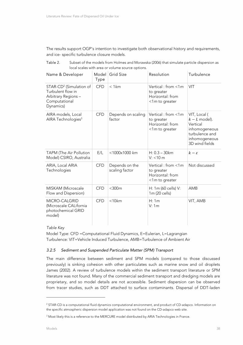
Literature Review: Fate of Dispersed Oil Under Ice
Models 38
The results support OGP's intention to investigate both observational history and requirements, and ice- specific turbulence closure models.
Table 2. Subset of the models from Holmes and Morawska (2006) that simulate particle dispersion as local scales with area or volume source options.
Name & Developer ModelType
Grid Size Resolution Turbulence
STAR-CD2 (Simulation of Turbulent flow in Arbitrary Regions – Computational Dynamics)
CFD < 1km Vertical : from <1m to greater Horizontal: from <1m to greater
VIT
AIRA models, Local AIRA Technologies3
CFD Depends on scaling factor
Vertical : from <1m to greater Horizontal: from <1m to greater
VIT, Local ( model).
Vertical inhomogeneous turbulence and inhomogeneous 3D wind fields
TAPM (The Air Pollution Model) CSIRO, Australia
E/L <1000x1000 km H: 0.3 – 30km V: <10 m
ARIA, Local ARIA Technologies
CFD Depends on the scaling factor
Vertical : from <1m to greater Horizontal: from <1m to greater
Not discussed
MISKAM (Microscale Flow and Dispersion)
CFD <300m H: 1m (60 cells) V: 1m (20 cells)
AMB
MICRO-CALGRID (Microscale CALifornia photochemical GRID model)
CFD <10km H: 1m V: 1m
VIT, AMB
Table Key Model Type: CFD =Computational Fluid Dynamics, E=Eulerian, L=Lagrangian Turbulence: VIT=Vehicle Induced Turbulence, AMB=Turbulence of Ambient Air
3.2.5 Sediment and Suspended Particulate Matter (SPM) Transport
The main difference between sediment and SPM models (compared to those discussed previously) is sinking cohesion with other particulates such as marine snow and oil droplets James (2002). A review of turbulence models within the sediment transport literature or SPM literature was not found. Many of the commercial sediment transport and dredging models are proprietary, and so model details are not accessible. Sediment dispersion can be observed from tracer studies, such as DDT attached to surface contaminants. Dispersal of DDT-laden
2 STAR-CD is a computational fluid dynamics computational environment, and product of CD-adapco. Information on the specific atmospheric dispersion model application was not found on the CD-adapco web site.
3 Most likely this is a reference to the MERCURE model distributed by ARIA Technologies in France.
Literature Review: Fate of Dispersed Oil Under Ice
Models 39
sediments has been observed for over two decades dispersing from entry points in the Southern California Bight, Zeng and Venkatesan,(1999). Bandara et al. (2011) and others have developed oil in sediment models, but are not immediately relevant to turbulence of oil in ice covered waters.
One model of sediment sinking and resuspension that is linked to a 3D operational circulation model found in Lou et al. (2000). The environmental inputs are circulation fields from a Lake Michigan implementation of the Princeton Ocean Model (POM) by Blumberg and Mellor (1987) and a simple 2D wind wave model for wave direction and significant wave heights (Schwab et al. 1984).
∙ Δ Δ ∙ Δ
Where , , , is the concentration of suspended sediment, , are the horizontal and vertical water velocities, is the sediment sinking rate, and , are the horizontal and vertical sediment diffusion coefficients.
In this case the full magnitude of the total current and wave mixing coefficient, , is given by the magnitude of the resulting vector for the horizontal current dispersion, , and the vertical wave dispersion, , such that . The POM turbulence closure scheme is used to calculate the horizontal current dispersion and the Bosman (1982) wave-induced sediment dispersion model is used for wave related sediment dispersion.
Modeling Gaps 3.3
3.3.1 Oil Droplets in a Turbulent IOBL
From a dynamical point of view, an emulsion of slightly buoyant oil droplets in a turbulent IOBL has several characteristics in common with frazil ice. IOBL models including frazil are usually based on similar approaches used for bottom sediment transport (Mellor et al. 1986; Omstedt; Svensson 1984; Sherwood 2000). Typically, 1-d models take the form
û û û
.. .. .. .. ..
where lower case subscripts denote differentiation, is the ratio of scalar eddy diffusivity to
eddy viscosity for each scalar (often taken as unity in a fully turbulent flow), , are volume
concentrations of different frazil crystal classes, with rise velocities, , , and , are the respective source terms for each frazil class. Adapting such a model to oil droplet classes would be important in simulating the effects of the shear layer and turbulence on the surface oil and droplet dispersion.
3.3.2 Oil in the Near-Shore, Ice Infested Environment
An ice-covered, shallow water environment includes factors that can change contaminant mixing and transport behaviour substantially. Ekman (1905) first elucidated the impact of coastal setup/setdown by showing that rightward volume transport associated with an alongshore
Literature Review: Fate of Dispersed Oil Under Ice
Models 40
stress will induce a pressure gradient perpendicular to the shoreline. If the alongshore wind persists long enough, a nearly steady state is possible where transport onshore (offshore) in the upper IOBL is balanced by offshore (onshore) transport in a bottom boundary layer, with the latter driven by an alongshore current in geostrophic balance with the perpendicular pressure gradient. This current, when combined with the downwind surface component in the IOBL, can easily double the alongshore surface velocity (and ice transport) relative to the IOBL surface current. For forcing with shore to the right (e.g., westerly winds along the North Slope of Alaska), the impact of strong wind is to drive water and ice toward shore, posing the risk of a damaging storm surge, or in some cases, a dangerous ice ride-up event (Shapiro; Metzner 1979). For opposite winds, surface drift is offshore, often opening water to cold air temperature, rapid freezing, and brine production. Modelling of ice and contaminant transport in the near-shore environment should account for these effects.
Vertical mixing in the near-shore environment is significantly altered by the addition of a turbulent bottom boundary layer. If the water column is stratified at the start of a wind event, a two-layer system tends to develop with increasing stress and geostrophic current. The upper and lower layers are often separated by a strong pycnocline that limits exchange between them, and that would tend to confine, e.g., oil droplets released near the bottom to the lower layer, provided their relative buoyancy was small. However, a combination of turbulence from shear at both boundaries and from surface freezing can rapidly erode the pycnocline leaving the water column well mixed from top to bottom, with large impact on surface manifestation and transport of such a contaminant. We note that a bottom-released contaminant with significant buoyancy (for example, by including a gaseous component) would mimic the mixing impact of freezing at the surface.
In shallow environments covered by fast ice, tidal currents are often the most significant factor in mixing and transport of water properties. Fast ice differs from freely drifting pack ice in that the upper boundary layer resists rather than drives the interior current. Many of the two-boundary-layer considerations mentioned above pertain, except that a contaminant that reaches the ice/water interface will probably stay close to its source region. In addition, after the initial phase of ice formation, freezing rates under fast ice will remain relatively slow compared to a regime with episodic ice removal by wind.
It is not uncommon to encounter fronts in temperature and salinity structure near the boundaries between fast and mobile pack ice, and near the mouths of ice covered fjords or bays (Skogseth et al. 2013). In addition to turbulence generated directly by shear instabilities, advected fronts can produce buoyancy flux of either sign by shearing of horizontal density gradients in the boundary layers, with large asymmetry in mixing depending on the direction of flow (Crawford et al. 1999; McPhee et al. 2013).
Turbulence in shallow water can also induce sediment transport, with the possibility of scavenging and subsequent bottom deposition of suspended oil droplets. Sherwood (2000) investigated a combined frazil/suspended sediment transport model for the Kara Sea. McPhee (1998a) formulated a combined radionuclide/sediment interaction model to investigate uptake of radionuclides in contaminated water by sediment binding. Given estimates of rate of binding of oil droplets to sediment particles, these concepts are applicable to oil scavenging.

Literature Review: Fate of Dispersed Oil Under Ice
Models 41
3.3.3 Impact of Oil at the Ice/Water Interface
With regard to the IOBL modelling discussed in section 2.1, several characteristics of the ice/water interface may be affected by oil in ways not well understood. Some outstanding issues are identified in the following.
3.3.3.1 Surface Roughness (drag) Introducing a layer of oil at the interface between a relatively compact ice cover and the IOBL may substantially modify the stress/velocity relationship, depending on many diverse factors, including the thickness and viscosity of oil comprising the intermediate layer and the spectrum of under-ice roughness morphology. Underside hydraulic roughness can differ by orders of magnitude, ranging from hydraulically smooth ∗⁄ ~10 for undeformed fast ice (Crawford et al. 1999), to ~0.1 m for heavily ridged multiyear pack ice (Shaw et al. 2008). The most significant modification may occur with smoother ice, since for a hydraulically smooth surface, drag depends on fluid viscosity rather than physical surface protrusions (Hinze 1975). Even in undeformed fast ice, estimates of the under- surface area covered by oil vary widely: from about half for methods assuming that oil collects in pools only in areas with ice thickness less than the median ice thickness, to about 8% in a model where oil is allowed to migrate between adjacent concavities as observed in under-ice morphology by multi-beam sonar measurements [Wilkinson et al., 2007]. One can picture, for example, a situation where oil that collected under fast (stationary) ice would modify the drag relationship with the underlying tidal or residual current by both “smoothing over” concavities left by differential freezing, and by changing the character of the under-ice surface covered by oil. This might substantially change the amount of turbulent mixing in the upper water column for a given current magnitude.
According to Lewis (1976b), there is a relatively large “sticking friction” between a drop or slick of oil and the ice base. He cites, for example, that a slope of at least 2% is required for oil to begin moving by gravitational force, and that oil remained adhered to the ice base in a current of 0.1 m s-1. He speculates that a current of at least 0.3 m s-1 is needed to start oil moving on a level surface. With regard to relative transport of oil along the ice base, or “re-emulsifying” the oil into the water column, incorporating these observations from stationary ice into a model of oil in moving pack ice presents a significant modelling (and observational) challenge. In the 1979-1980 field experiments in McKinley Bay, Canada, oil and gas collected in depressions under the ice, and flowed gravitationally along the underside of the ice until reaching an equilibrium distribution (Dickens et al. 1981). Releases were in December 1979 and April 1980.
3.3.3.2 Heat and Salt Exchange during Rapid Melting Melting of sea ice depends on a delicate interplay between the transfer of salt and heat through thin sub- layers directly adjacent to the ice/water interface. Field observations indicate that in addition to friction velocity and far-field values of and , melt rate depends on a combination of Prandtl and Schmidt numbers, i.e., on thermal and haline molecular diffusivities, with diffusion of salt into the ice lattice controlling the process. Molecular diffusivity of salt in liquid is inversely proportional to fluid viscosity, so a layer of oil (much higher viscosity than seawater (Al-Besharah et al. 1987)) between the ice and water may substantially slow basal melt by inhibiting salt transfer. Since melt rate also depends directly on ∗, extrapolating from laboratory studies may be difficult unless conditions similar to those found in the field can be reproduced.
Literature Review: Fate of Dispersed Oil Under Ice
Models 42
3.3.3.3 Oil Impact during Freezing According to Feltham et al. (2006), sea ice is a “mushy layer” comprising a reactive porous medium with two phases and two components. Although there exists considerable theoretical work on brine expulsion from growing sea ice (Notz; Worster 2009; Wells et al. 2011; Wettlaufer et al. 1997), in recent work Rees Jones; Worster (2013) emphasize the vertical upwelling velocity within the ice matrix, and model the matrix as a way of determining rather than prescribing the salinity profile in the ice. How oil would be incorporated into this framework to predict its migration into the growing ice column presents an interesting and germane problem from both modelling and observational perspectives.
The thermal conductivity of ice is several times greater than oil, thus a layer of oil separating ice from water inhibits ice growth compared with surrounding uncontaminated ice. Lewis (1976b) describes observations under fast ice with a figure illustrating how this effect produces a “lip” surrounding an oil pool under fast ice, thus further restricting oil migration. Brine drainage continued allowing penetration of oil “a few cm up into the ice sheet.”During the Canadian field trials in 1979 and 1980, rapid encapsulation of oil and/or gas occurred as late as May (Dickens et al. 1981). The oil was released from the ice the next spring, emerging primarily from ice sheet ablation, but also through brine channel migration.
3.3.3.4 Role of False Bottoms in Dispersal and Migration of Oil By the end of the summer melt season, the multiyear pack ice column often contains multiple layers of nearly fresh water sandwiched between thin layers of ice. These apparently form when meltwater collects in under-ice concavities (“bottom melt ponds”), and then forms a thin layer of fresh ice where the fresh water (at 0 °C) overlies seawater (typically -1.5 to -1.8 °C). During times of significant stress (elevated ) the ice layer migrates upward in response to double-diffusive forcing (Notz et al. 2003), leaving a cavity that may again fill with fresh water. At an AIDJEX station in 1975, A. Hanson found that by this mechanism, initially thin ice would increase in thickness over the course of the summer while thick ice thinned as expected. In an environment with oil near the interface at the onset of melting, this process (if undisturbed) could conceivably incorporate significant amounts of oil into the ice column during melting, in a way not otherwise anticipated.
False bottoms as described above occur during summer as fresh water from surface and interior melting makes its way down through the water column. Interestingly, a similar process is described in the study mentioned above (Lewis 1976b) of a pool of oil placed under 1.6-m thick fast ice as the ice was growing in March. After about a week, ice began to grow beneath the oil pool, eventually reaching a thickness of 10-20 cm, completely encapsulating the lens. Lewis points out that this oil will eventually reach the ice surface with little change in its chemical properties.
3.3.4 The Marginal Ice Zone
One of the most challenging modelling gaps is consistent treatment of marginal ice zones, where open ocean conditions transition to ice covered. In the former, momentum flux and TKE production and transport in the OBL are modified substantially by surface gravity waves, while surface fluxes are dominated by heat, water vapour, and other constituent gas transfers (including volatiles) at a gas/water interface. At the solid ice-ocean interface, momentum transfer depends on physical roughness elements and scalar fluxes depend on sensible and latent exchanges at a solid/liquid boundary. Although most modelling approaches treat a
Literature Review: Fate of Dispersed Oil Under Ice
Models 43
mixture of ice and water with weighted averages of the respective exchange coefficients, measurements show atmospheric drag in the MIZ to be larger than either the open ocean or pack ice (except rubble fields) (Guest; Davidson 1991a). Similarly, observations of ocean drag in the MIZ are consistently high relative to all but the roughest pack ice (cf. section 1.1.2).
Stokes drift associated with large amplitude surface waves (swell), and associated Langmuir circulation, is a significant factor in the open OBL (Mcwilliams et al. 1997; Plueddemann et al. 1996), but probably has little impact in the IOBL. On the other hand, even in the absence of surface waves, convection from rapid freezing creates quasi-organized rolls that greatly increase effective eddy viscosity (McPhee; Stanton 1996). In a MIZ with cold, off-ice winds, strong convection may provide a roll structure analogous to Langmuir circulations in the OBL, enhancing mixing, and including herding of ice fragments and surface contaminants in windrows. Conversely, as discussed in section 2.1.3, when ice is blown toward warm water, drag is reduced substantially, and ice divergence may result as ice trailing the leading edge encounters cooled (by melting) water. The impact of orbital wave velocities on melting and freshwater flux in the MIZ needs better theoretical/modelling description.
Except under extreme circumstances (e. g., polar lows in the Southern Ocean), ocean swell directed toward an ice edge will attenuate in amplitude exponentially over relatively short distances (Wadhams et al. 1988). That contaminants transported near the surface of the open ocean by Stokes drift would concentrate in the MIZ by transport convergence as the wave energy dropped on encountering ice is plausible as oil collects at the boundary between unmixed fresh water discharge and the ocean. Convergence of wave driven transport along the California coast during significant swell events has been associated with high phytoplankton concentrations (“blooms”) (McPhee-Shaw et al. 2011).
3.3.5 Changing Ocean Circulation in the Arctic
Most of this chapter has concentrated on the IOBL, and its currents relative to the “undisturbed” water column beyond the frictional boundary layers. Away from the shallow water and the continental shelves, the undisturbed ocean velocity is usually considered to be the surface geostrophic velocity, proportional to the gradient of sea-surface elevation, with the total surface velocity being the vector sum of the IOBL surface velocity and the geostrophic current. In the Canada Basin, the major ocean circulation feature is the clockwise rotating (anticyclonic) Beaufort Gyre. In the past, currents associated with the Gyre have been relatively small (at most a few centimeters per second), but persistent in that ice islands like T3 would make multiple circuits, each taking several years, before becoming entrained in the transpolar drift stream and exiting the Arctic via Fram Strait.
Over the past decade, the well-publicized changes in Arctic sea ice extent and thickness have been accompanied by lesser known, but no less alarming changes in Arctic Ocean circulation, resulting from a large increase and redistribution of liquid freshwater (McPhee 2013; McPhee et al. 2009). A dynamic topography compiled from hydrographic measurements in the Canada Basin from 2008 through 2011, including daily Ice-Tethered Profiler (ITP) data in every season, indicates that the speed of geostrophic currents offshore from the Beaufort and Chukchi continental slopes is now as much as 5-6 times greater than speeds based on the most recently published climatology (PHC 3.0, Steele et al. 2001), representative of conditions up to about 2000. By integrating tangential velocities about a circle inscribed within the domain of the
Literature Review: Fate of Dispersed Oil Under Ice
Models 44
Beaufort Gyre, we find that whereas a circuit with geostrophic velocities computed from PHC 3.0 would require about 5 years, this now takes slightly over a year.
Summary 3.4
Based on the literature review above, careful selection of the turbulence closure model and environmental input data (i.e. currents and waves) are keys to predictive success (e.g. Holmes; Morawska (2006). The literature of particle simulations in Eulerian flows covers a wide range of topics, from larval fish, oil and other contaminants, intentional tracer releases, sediments and SPM. The model provided is expected to be valid in greater than 90% ice cover, as the IOBL will continue to behave as if ice covered, and perhaps as low as 75% ice cover. There is potential to be valid at even lower ice coverage, as experience during the AIDJEX experiment shows ice cover as low as 25% was only different in the absorption of solar radiation (Maykut; McPhee 1995).

Literature Review: Fate of Dispersed Oil Under Ice
Overall Summary, Analysis and Recommendations 45
CHAPTER 4. OVERALL SUMMARY, ANALYSIS AND RECOMMENDATIONS
The literature review supports the view that sufficient knowledge exists to develop an under-ice turbulence closure model, but that existing observations are probably not good enough to provide both calibration and verification data. The mixing of oil droplets in nature differs significantly from the dispersion of ichthyoplankton and other nearly neutrally buoyant particles and tracers. Surfacing oil droplets change character to sheens and slicks. These require energy to disperse back into the water column, and the resulting droplet sizes may in general not be the same as those that created the surface expression.
The fate of an isolated cloud of oil droplets under ice depends essentially on the droplet size distribution and the vertical turbulence profile. The longer the droplets are retained in the water column, the more the droplet cloud will become diluted due to horizontal mixing, and the more the oil will biodegrade. The smallest oil droplets that resurface under the ice will also not tend to reform into larger slicks or pools, to the extent that the average inter-droplet distance exceeds the mean horizontal distance between under-ice roughness elements. For more continuous subsurface sources of oil and/or gas, the oil and/or gas can collect under the ice, with the thickness dependent on the oil's density and surface tension (Lewis 1976a). Field tests in 1979-1980 with oil and gas released at ~20 depth showed the larger droplets collecting under the ice within 50 of the plume centerline, slightly smaller droplets collecting within 350 of the plume centerline (Dickens et al. 1981). The underside of the ice changed over the winter, and by April more waves and packets were created on the underside of the ice for oil and gas to collect within, thus changing the initial distribution of oil under the ice.
Ice exists in a wide variety of ice types, morphologies, and characteristics: thickness, degree of coverage, floe size, porosity, and so forth. The major categories of ice are discussed briefly earlier in this report. To the extent that these differences contribute to changes in the under-ice turbulence profile for a given met- ocean (wind-current-wave) regime, the differences are relevant to the problem being addressed here.
There are many possible observational strategies for improving and evaluating our ability to model the fate potential for an oil patch to remain suspended in the water column which will be determined by the particular ice-regime of interest along with other environmental parameters as well as cost and personnel safety. Below is a short list based on successful field studies in the past.
Fluorescent Dyes: We suggest that in the sea ice or in a rubble field, aerial surveys of fluorescent dyes might be useful for the determination of the resurfacing potential of dispersed oil, provided that an injection of fluid of the correct buoyancy could be accomplished. It is envisioned that such an approach might be applicable for small time and space scale studies.
Turbulent Instrument Cluster: For pack or drift ice characterized by large stable floes, turbulent instrument clusters (TICs) remain the preferred instrument package. Caveats include the fact that such environments can be spatially heterogeneous so that a relatively small number of TICs may be inadequate to sample the small-scale variability of turbulence regimes near ridges and keels.
Autonomous Underwater Vehicles: Powered AUVs are potentially good platforms for measuring turbulence in the IOBL, particularly when combined with measurements of ice draft with sonar, and could prove useful for measuring turbulence in the IOBL. Their maneuverability allows investigators to respond to observed spatial and temporal changes
Literature Review: Fate of Dispersed Oil Under Ice
Overall Summary, Analysis and Recommendations 46
in the met-ocean-ice environment. AUVs could potentially be deployed in a broad range of ice concentrations provided adequate vessel support was available. The downside is that the instrumentation is costly and risks can be high. Also, AUVs cannot sample into the log-layer very close to the under-ice boundary that may be important for oil spreading and local enhancement of turbulence. Powered AUV operations in heavy ice cover are becoming more routine, with under-ice topography from single or multi-beam sonar an essential component of the operations. AUVs typically have mission lives measured in hours so that operators have to be directly on hand with vessel or ice-camp support.
Acoustic Doppler Current Profilers (ADCPs): A relatively high frequency ADCP can be suspended beneath the ice to capture the turbulence profile in the first few meters of the water column. An accompanying lower frequency instrument could be used to record velocities over a greater depth, but without the same temporal detail.
Passive traces such as flourescene and rhodamine: These are potentially useful for increased tracking of an experimental oil droplet plume, and for estimation of gross vertical and horizontal dispersion rates.
Based on the literature review, we offer the recommendations below for selection of a turbulence model to implement and prioritization strategies for field work required to support model calibration, verification and use.
Turbulence Model Selection 4.1
No off-the-shelf model exists that can be easily adapted to the variety of ice types and concentrations that could be encountered during a spill where oil dispersal (chemical or mechanical) is required. Adaptation of the McPhee (2008) first order closure model based on the literature review is recommended for implementation as a next generation model. Our reasoning is as follows:
LTC is based on combining turbulence similarity theory with extensive direct measurements of turbulence characteristics in the under ice boundary layer under widely varying conditions of ice types and physical forcing (stress, heat and salt fluxes).
In contrast to slab (mixed-layer) models, a model incorporating LTC provides vertical profiles of turbulence properties critical for determining the fate of oil droplets in the water column: Reynolds stress, buoyancy flux, eddy viscosity/diffusivity, as well as TKE production and dissipation. LTC and KPP 1st order closures include the high shear region near the interface explicitly, rather than considering it separately. It is important that shear in the outer part of the IOBL is acknowledged since it means oil will be transported in quite different directions depending on distance from the boundary.
An LTC model also provides realistic vertical velocity profiles that are fundamentally shaped by rotational (Coriolis) forces, critical for determining the speed and direction of droplet motion at different levels in the water column.
Real-time forecast implementation of LTC is relatively straightforward. An onboard model incorporating meteorological forecasts and ice-concentration imagery was used daily with good results during the MaudNESS project in the Weddell Sea, Antarctica, and has been included as part of a major tracer-tracking experiment proposed for the Arctic (IDEAr).
Literature Review: Fate of Dispersed Oil Under Ice
Overall Summary, Analysis and Recommendations 47
LTC is readily adaptable to specific local conditions including: energetic inertial oscillation (cycloidal ice motion); shallow environments with or without stratification; complications posed by frazil generation, and/or sediment transport.
Model Input Requirements 4.2
Given our present capabilities, the following measurements could reasonably be made on a spill response timescale:
Wind
Droplet size distribution (noted as a given by the TWG)
Ice Type → proxy for bottom roughness
Ice Concentration
Turbulence Profile
Velocity Profile
From the input data above, the final model would provide guidance on the likelihood of oil resurfacing. In planning the field program and details of the model development (sections 4.1 and 4.3) we may determine a need to collect additional field data alongside the above listed parameters to ensure that the implemented model is fully calibrated and functional.
Prioritization of Ice Types in Field Study 4.3
Most measurements of turbulence in the upper ocean (0 to 15m) in a polar environment derive from studies by McPhee and collaborators that have been made from the stable platform provided by pack ice. Hence we know far more about the consolidated MY pack ice than lower ice concentration conditions. Worth noting is that some of these measurements have occurred at the edges of leads (e.g. LEADEX). (Guest; Davidson 1991b), and (Guest et al. 1995b), discuss enhanced wind drag in MIZs, which is mirrored by enhanced under ice roughness, e.g.(Johannessen 1970; McPhee et al. 1990; Pease et al. 1983). Consequently, there is a tradeoff between less impact from surface gravity waves versus direct enhanced momentum transfer from the wind. We suggest that wind stress transfer to the ocean peaks somewhere between 40-80% ice concentration, due to form drag of the pack in free drift. Field measurements could provide more information for modeling turbulence regimes in the transition region between pack ice and the MIZ.
Specifically under-represented conditions are:
1) Loose rubble fields or conditions where floe sizes are small. Such conditions might be found in the Marginal Ice Zone, or where the ice pack is actively deforming, rafting and ridging, or in coastal polynias where older ice is transported away from the coast such that there is a loose zone of ice pack.
2) Areas at the onset of ice growth in the open ocean (e.g. the Chukchi and Barents Seas). 3) Drift of the ice edge or MIZ into another region (e.g. summer Beaufort, or Barents Seas)
could be similar to the ice rubble field if managed ice is the main source of the field. This may be the most likely scenario for spills in operational oil development areas, and so should have associated field measurements for model calibration.

Literature Review: Fate of Dispersed Oil Under Ice
Overall Summary, Analysis and Recommendations 48
From the perspective of balancing the cost of field measurements with the slow development of oil reserves in the Arctic, this list of ice types could be reorganized based on the ice conditions found where oil development is currently proceeding. This prioritization could be done through a study of ice types based on remote sensing data from oil development areas. The goal would set a priority list to first fill in knowledge gaps in ice types from areas where a potential spill could occur.
One key point in need of resolution is the transition from the subsurface stability regime found under pack ice to that of open water. Measurements by McPhee and collaborators indicate that in the MIZ, there is a range of ice concentrations where the underlying turbulence regime could be more like open water or more like pack ice.
Literature Review: Fate of Dispersed Oil Under Ice
References 49
CHAPTER 5. REFERENCES
Al-Besharah, J. M., O. A. Salman, and S. A. Akashah, 1987: Viscosity of crude oil blends. Industrial & Engineering Chemistry Research, 26, 2445-2449.
ASCE, 1996: ASCE Task Committee on Modeling of Oil Spills of the Water Resources Engineering Division. ASCE Journal of Hydraulic Engineering, 122, 594-609.
Bandara, U. C., and P. D. Yapa, 2011: Bubble Sizes, Breakup, and Coalescence in Deepwater Gas/Oil Plumes. Journal of Hydraulic Engineering, 137, 729-738.
Bandara, U. C., P. D. Yapa, and H. Xie, 2011: Fate and transport of oil in sediment laden marine waters. Journal of Hydro-environment Research, 5, 145-156.
Barenblatt, G. I., 1996: Scaling, self-similarity, and intermediate asymptotics. Cambridge University Press, xv, 386 p. pp.
Batchelor, G. K., 1967: The Theory of Homogeneous Turbulence. Cambridge University Press, 197 pp. Bauer, J., and S. Martin, 1980: Field Observations of the Bering Sea Ice Edge Properties during March 1979. Monthly Weather Review, 108, 2045-2056.
Baumert, H. Z., . Simpson, and . r. S ndermann, 2005 Marine turbulence : theories, observations, and models. Cambridge University Press, xxi, 630 p. pp.
Bechtel, R. D., E. Wickley-Olsen, M. C. Boufadel, J. Weaver, and C. H. Barker, 2008: The movement of oil at sea due to irregular waves. International Oil Spill Conference, Savannah, Georgia, USA, May 4-8, 2008, Allen Press, 943-947.
Blackadar, A. K., and H. Tennekes, 1968: Asymptotic Similarity in Neutral Barotropic Planetary Boundary Layers. Journal of the Atmospheric Sciences, 25, 1015-1020.
Blumberg, A. F., and G. L. Mellor, 1987: A description of a three-dimensional coastal ocean circulation model. Coastal and estuarine sciences, 4, 1-16.
Bosman, J., 1982: Concentration measurements under oscillatory motion. M1695-II and M, 1875. Boufadel, M. C., R. D. Bechtel, and J. Weaver, 2006: The movement of oil under non-breaking waves. Marine Pollution Bulletin, 52, 1056-1065.
Bowden, K., 1965: Horizontal mixing in the sea due to a shearing current. Journal of Fluid Mechanics, 21, 83-95.
Buckley, J. R., T. Gammelsrød, J. A. Johannessen, O. M. Johannessen, and L. P. Røed, 1979: Upwelling: Oceanic Structure at the Edge of the Arctic Ice Pack in Winter. Science, 203, 165-167. Cearex_Drift_Group, 1990: CEAREX Drift Experiment. Eos, Transactions American Geophysical Union, 71, 1115-1118.
Chant, R. J., and Coauthors, 2008: Dispersal of the Hudson River Plume in the New York Bight Synthesis of Observational and Numerical Studies During LaTTE. Oceanography, 21, 148-161.
Clarke, R. H., and G. D. Hess, 1974: Geostrophic departure and the functions A and B of Rossby-number similarity theory. Boundary-Layer Meteorol, 7, 267-287.
Cole, S., M. L. Timmermans, J. M. Toole, R. A. Krishfield, and F. T. Thwaites, 2012: Ekman veering, internal waves, and turbulence observed under Arctic sea-ice (In revision). Journal of Physical Oceanography.
Collins, W. D., and Coauthors, 2006: The Community Climate System Model Version 3 (CCSM3). Journal of Climate, 19, 2122-2143.
Crawford, G., L. Padman, and M. G. McPhee, 1999: Turbulent mixing in Barrow Strait. Continental Shelf Research, 19, 205-245.
Dasaro, E. A., and J. H. Morison, 1992: Internal Waves and Mixing in the Arctic-Ocean. Deep-Sea Res, 39, S459-S484.
Deardorff, J. W., 1974: Three-dimensional numerical study of turbulence in an entraining mixed layer. Boundary-Layer Meteorology, 7, 199-226.
Dickens, D. F., I. A. Buist, and W. M. Pistruzak, 1981: Dome's Petroleum Study of Oil and Gas Under Sea Ice. International Oil Spill Conference, IOSC.
Literature Review: Fate of Dispersed Oil Under Ice
References 50
Dowdeswell, J. A., and Coauthors, 2008: Instruments and MethodsAutonomous underwater vehicles (AUVs) and investigations of the iceocean interface in Antarctic and Arctic waters. Journal of Glaciology, 54, 661-672.
Ekman, V. W., 1905: On the influence of the earths rotation on ocean currents. Ark. Mat. Astr. Fys., 2, 1-52. Feltham, D. L., N. Untersteiner, J. S. Wettlaufer, and M. G. Worster, 2006: Sea ice is a mushy layer. Geophysical Research Letters, 33, L14501.
Fer, I., R. Skogseth, and F. Geyer, 2010: Internal Waves and Mixing in the Marginal Ice Zone near the Yermak Plateau. Journal of Physical Oceanography, 40, 1613-1630.
Fischer, H. B., 1972: Mass transport mechanisms in partially stratified estuaries. J. Fluid Mech, 53, 671-687.
——, 1979: Mixing in inland and coastal waters. Academic Pr.
Gargett, A. E., 1994: Observing Turbulence with a Modified Acoustic Doppler Current Profiler. Journal of Atmospheric and Oceanic Technology, 11, 1592-1610.
Gerbi, G. P., J. H. Trowbridge, E. A. Terray, A. J. Plueddemann, and T. Kukulka, 2009: Observations of Turbulence in the Ocean Surface Boundary Layer: Energetics and Transport. Journal of Physical Oceanography, 39, 1077-1096.
Geyer, W. R., R. Chant, and R. Houghton, 2008: Tidal and spring-neap variations in horizontal dispersion in a partially mixed estuary. J Geophys Res-Oceans, 113.
Gill, A. E., 1982: Atmosphere-ocean dynamics. Academic Press, xv, 662 p. pp.
Goodman, L., E. R. Levine, and R. G. Lueck, 2006: On measuring the terms of the turbulent kinetic energy budget from an AUV. Journal of Atmospheric and Oceanic Technology, 23, 977-990.
Gordon, A. L., I. Ice Station Weddell Group of Principal, and S. Chief, 1993: Weddell Sea exploration from ice station. Eos, Transactions American Geophysical Union, 74, 121-126.
Grant, H. L., R. W. Stewart, and A. Moilliet, 1962: Turbulence spectra from a tidal channel. Journal of Fluid Mechanics, 12, 241-268.
Gregg, M. C., E. A. D'Asaro, T. J. Shay, and N. Larson, 1986: Observations of Persistent Mixing and Near- Inertial Internal Waves. Journal of Physical Oceanography, 16, 856-885.
Guest, P. S., and K. L. Davidson, 1991a: The aerodynamic roughness of different types of sea ice. Journal of Geophysical Research: Oceans, 96, 4709-4721.
Guest, P. S., and K. L. Davidson, 1991b: The aerodynamic roughness of different types of sea ice. Journal of Geophysical Research: Oceans (1978–2012), 96, 4709-4721.
Guest, P. S., J. W. Glendening, and K. L. Davidson, 1995a: An observational and numerical study of wind stress variations within marginal ice zones. Journal of Geophysical Research: Oceans, 100, 10887-10904. Guest, P. S., J. W. Glendening, and K. L. Davidson, 1995b: An observational and numerical study of wind stress variations within marginal ice zones. Journal of Geophysical Research: Oceans (1978–2012), 100, 10887-10904.
Harcourt, R. R., 2005: Thermobaric cabbeling over Maud Rise: Theory and large eddy simulation. Progress in Oceanography, 67, 186-244.
Hayes, D. R., and J. H. Morison, 2002: Determining Turbulent Vertical Velocity, and Fluxes of Heat and Salt with an Autonomous Underwater Vehicle. Journal of Atmospheric and Oceanic Technology, 19, 759-779.
Hibler, W. D., 1979: A Dynamic Thermodynamic Sea Ice Model. Journal of Physical Oceanography, 9, 815-846.
Hinze, J. O., 1975: Turbulence. 2d ed. McGraw-Hill, x, 790 p. pp.
Holmes, N. S., and L. Morawska, 2006: A review of dispersion modeling and its application to the dispersion of particles: An overview of different dispersion models available. Atmospheric Environment, 40, 5902-5928.
Houghton, R. W., R. J. Chant, A. Rice, and C. Tilburg, 2009: Salt flux into coastal river plumes: Dye studies in the Delaware and Hudson River outflows. J Mar Res, 67, 731-756.

Literature Review: Fate of Dispersed Oil Under Ice
References 51
Hunkins, K., 1966: Ekman drift currents in the Arctic Ocean. Deep Sea Research and Oceanographic Abstracts, 13, 607-620.
——, 1967: Inertial oscillations of Fletcher's Ice Island (T-3). Journal of Geophysical Research, 72, 1165-1174.
Hyatt, J., 2006: Wind, Sea Ice, Inertial Oscillations and Upper Ocean Mixing in Marguerite Bay, Western Antarctic Peninsula: Observations and Modeling, MIT/WHOI Joint Program, 171 pp.
Häkkinen, S., and G. L. Mellor, 1992: Modeling the seasonal variability of a coupled Arctic ice-ocean system. Journal of Geophysical Research: Oceans, 97, 20285-20304.
Incropera, F. P., and D. P. DeWitt, 1985: Fundamentals of Heat and Mass Transfer, Second Edition. John Wiley & Sons, 802 pp.
James, I., 2002: Modelling pollution dispersion, the ecosystem and water quality in coastal waters: a review. Environmental Modelling & Software, 17, 363-385.
Johannessen, O. M., 1970: Note on some vertical profiles below ice floes in the Gulf of St. Lawrence and near the North Pole. Journal of Geophysical Research, 75, 2857-2861.
Johannessen, O. M., J. A. Johannessen, J. H. Morison, B. A. Farrelly, and E. A. S. Svendsen, 1983: Oceanographic conditions in the marginal ice zone north of Svalbard in early fall 1979 with an emphasis on mesoscale processes. Journal of Geophysical Research: Oceans, 88, 2755-2769.
Josberger, E. G., 1983: Sea ice melting in the marginal ice zone. Journal of Geophysical Research: Oceans, 88, 2841-2844.
Kantha, L. H., and G. L. Mellor, 1989: A two-dimensional coupled ice-ocean model of the Bering Sea marginal ice zone. Journal of Geophysical Research, 94, 10921.
Kay, J. E., M. M. Holland, and A. Jahn, 2011: Inter-annual to multi-decadal Arctic sea ice extent trends in a warming world. Geophysical Research Letters, 38, L15708.
Kraus, E. B., and J. S. Turner, 1967: A one-dimensional model of the seasonal thermocline II. The general theory and its consequences. Tellus, 19, 98-106.
Krishfield, R., J. Toole, A. Proshutinsky, and M. L. Timmermans, 2008: Automated Ice-Tethered Profilers for Seawater Observations under Pack Ice in All Seasons. Journal of Atmospheric and Oceanic Technology, 25, 2091-2105.
Langleben, M. P., 1982: Water drag coefficient of first-year sea ice. Journal of Geophysical Research: Oceans, 87, 573-578.
Large, W. G., J. C. McWilliams, and S. C. Doney, 1994: Oceanic vertical mixing: A review and a model with a nonlocal boundary layer parameterization. Reviews of Geophysics, 32, 363-403.
LeadEx_Group, 1993: The LeadEx experiment. Eos, Transactions American Geophysical Union, 74, 393-397.
Ledwell, J. R., and A. J. Watson, 1991: The Santa-Monica Basin Tracer Experiment - a Study of Diapycnal and Isopycnic Mixing. J Geophys Res-Oceans, 96, 8695-8718.
Ledwell, J. R., A. J. Watson, and C. S. Law, 1998: Mixing of a tracer in the pycnocline. J Geophys Res- Oceans, 103, 21499-21529.
Lenn, Y. D., and Coauthors, 2009: Vertical mixing at intermediate depths in the Arctic boundary current. Geophysical Research Letters, 36, L05601.
Lettau, H. H., 1979: Wind and temperature profile prediction for diabatic surface layers including strong inversion cases. Boundary-Layer Meteorol, 17, 443-464.
Levine, E. R., L. Goodman, and J. O'Donnell, 2009: Turbulence in coastal fronts near the mouths of Block Island and Long Island Sounds. Journal of Marine Systems, 78, 476-488.
Levine, M. D., C. A. Paulson, and J. H. Morison, 1985: Internal Waves in the Arctic Ocean: Comparison with Lower-Latitude Observations. Journal of Physical Oceanography, 15, 800-809.
Levine, M. D., L. Padman, R. D. Muench, and J. H. Morison, 1997: Internal waves and tides in the western Weddell Sea: Observations from Ice Station Weddell. Journal of Geophysical Research: Oceans, 102, 1073-1089.
Literature Review: Fate of Dispersed Oil Under Ice
References 52
Lewis, E., 1976a: Oil in sea ice. PACIFIC MARINE SCIENCE REPORT 76-12, JUNE 1976. 26 P, 12 FIG.
Lewis, E. L., 1976b: Oil in Sea Ice.
Lohrmann, A., B. Hackett, and L. P. Røed, 1990: High Resolution Measurements of Turbulence, Velocity and Stress Using a Pulse-to-Pulse Coherent Sonar. Journal of Atmospheric and Oceanic Technology, 7, 19-37.
Lou, J., D. J. Schwab, D. Beletsky, and N. Hawley, 2000: A model of sediment resuspension and transport dynamics in southern Lake Michigan. Journal of Geophysical Research: Oceans (1978–2012), 105, 6591-6610.
Lu, Y., and R. G. Lueck, 1999: Using a Broadband ADCP in a Tidal Channel. Part II: Turbulence. Journal of Atmospheric and Oceanic Technology, 16, 1568-1579.
Lueck, R., F. Wolk, and H. Yamazaki, 2002: Oceanic velocity microstructure measurements in the 20th Century. Journal of Oceanography, 58, 153-174.
MacKinnon, J. A., and M. C. Gregg, 2003: Shear and Baroclinic Energy Flux on the Summer New England Shelf. Journal of Physical Oceanography, 33, 1462-1475.
Martin, S., P. Kauffman, and C. Parkinson, 1983: The movement and decay of ice edge bands in the winter Bering Sea. Journal of Geophysical Research: Oceans, 88, 2803-2812.
Matsumoto, K., and Coauthors, 2004: Evaluation of ocean carbon cycle models with data-based metrics. Geophysical Research Letters, 31, L07303.
Maykut, G., and M. G. McPhee, 1995: Solar heating of the Arctic mixed layer. Journal of geophysical research, 100, 24691-24624,24703.
McPhee-Shaw, E. E., K. J. Nielsen, J. L. Largier, and B. A. Menge, 2011: Nearshore chlorophyll-a events and wave-driven transport. Geophysical Research Letters, 38, L02604.
McPhee, M. G., 1978: A simulation of inertial oscillation in drifting pack ice. Dynamics of Atmospheres and Oceans, 2, 107-122.
——, 1980: An Analysis of Pack Ice Drift in Summer. Sea Ice Processes and Models, R. S. Pritchard, Ed. University of Washington Press, 62-75.
——, 1981: An analytic similarity theory for the planetary boundary layer stabilized by surface buoyancy. Boundary-Layer Meteorol, 21, 325-339.
——, 1983a: Greenland sea ice/ocean margin. Eos, Transactions American Geophysical Union, 64, 82-83.
——, 1983b: Turbulent heat and momentum transfer in the oceanic boundary layer under melting pack ice. Journal of Geophysical Research: Oceans, 88, 2827-2835.
——, 1988: Analysis and Prediction of Short-Term Ice Drift. Journal of Offshore Mechanics and Arctic Engineering, 110, 7.
——, 1992a: Turbulent heat flux in the upper ocean under sea ice. J. Geophys. Res., 97, 5365-5379.
——, 1992b: Turbulent heat flux in the upper ocean under sea ice. Journal of Geophysical Research: Oceans, 97, 5365-5379.
——, 1994a: On the Turbulent Mixing Length in the Oceanic Boundary Layer. Journal of Physical Oceanography, 24, 2014-2031.
——, 1994b: On the Turbulent Mixing Length in the Oceanic Boundary-Layer. Journal of Physical Oceanography, 24, 2014-2031.
——, 1998a: A Numerical Sediment-Radionuclide Interaction Model for the Continental Shelf.
——, 1998b: An inertial-dissipation method for estimating turbulent flux in buoyancy-driven, convective boundary layers. Journal of Geophysical Research: Oceans, 103, 3249-3255.
——, 1999: Parameterization of mixing in the ocean boundary layer. Journal of Marine Systems, 21, 55-65.
——, 2002: Turbulent stress at the ice/ocean interface and bottom surface hydraulic roughness during the SHEBA drift. Journal of Geophysical Research: Oceans, 107, 8037.
Literature Review: Fate of Dispersed Oil Under Ice
References 53
——, 2004: A Spectral Technique for Estimating Turbulent Stress, Scalar Flux Magnitude, and Eddy Viscosity in the Ocean Boundary Layer under Pack Ice. Journal of Physical Oceanography, 34, 2180-2188.
——, 2008a: Air-ice-ocean interaction turbulent ocean boundary layer exchange processes. Springer, 215 pp.
——, 2008b: Physics of early summer ice/ocean exchanges in the western Weddell Sea during ISPOL. Deep Sea Research Part II: Topical Studies in Oceanography, 55, 1075-1097.
——, 2008c: Air-Ice-Ocean Interaction: Turbulent ocean boundary layer exchange processes. Springer, ix, 215 p. pp.
——, 2012: Advances in understanding ice–ocean stress during and since AIDJEX. Cold Regions Science and Technology, 76–77, 24-36.
——, 2013: Intensification of Geostrophic Currents in the Canada Basin, Arctic Ocean. Journal of Climate, 26, 3130-3138.
McPhee, M. G., and J. D. Smith, 1976: Measurements of the Turbulent Boundary Layer under Pack Ice. Journal of Physical Oceanography, 6, 696-711.
McPhee, M. G., and L. H. Kantha, 1989: Generation of internal waves by sea ice. Journal of Geophysical Research: Oceans, 94, 3287-3302.
McPhee, M. G., and D. G. Martinson, 1994: Turbulent Mixing Under Drifting Pack Ice in the Weddell Sea. Science, 263, 218-221.
McPhee, M. G., and T. P. Stanton, 1996: Turbulence in the statically unstable oceanic boundary layer under Arctic leads. Journal of Geophysical Research: Oceans, 101, 6409-6428.
McPhee, M. G., G. A. Maykut, and J. H. Morison, 1987: Dynamics and thermodynamics of the ice/upper ocean system in the marginal ice zone of the Greenland Sea. Journal of Geophysical Research: Oceans, 92, 7017-7031.
McPhee, M. G., D. Coefiicients, and U.-I. Roughness, 1990: 6 Small-Scale Processes.
McPhee, M. G., C. Kottmeier, and J. H. Morison, 1999: Ocean Heat Flux in the Central Weddell Sea during Winter. Journal of Physical Oceanography, 29, 1166-1179.
McPhee, M. G., J. H. Morison, and F. Nilsen, 2008: Revisiting heat and salt exchange at the ice-ocean interface: Ocean flux and modeling considerations. Journal of Geophysical Research: Oceans, 113, C06014. McPhee, M. G., T. Kikuchi, J. H. Morison, and T. P. Stanton, 2003: Ocean-to-ice heat flux at the North Pole environmental observatory. Geophysical Research Letters, 30.
McPhee, M. G., R. Kwok, R. Robins, and M. Coon, 2005: Upwelling of Arctic pycnocline associated with shear motion of sea ice. Geophysical Research Letters, 32, L10616.
McPhee, M. G., R. Skogseth, F. Nilsen, and L. H. Smedsrud, 2013: Creation and tidal advection of a cold salinity front in Storfjorden. Part 2: Supercooling induced by turbulent mixing of cold water.
McPhee, M. G., A. Proshutinsky, J. H. Morison, M. Steele, and M. B. Alkire, 2009: Rapid change in freshwater content of the Arctic Ocean. Geophysical Research Letters, 36, L10602.
McPhee, M. G., and Coauthors, 1996: The Antarctic Zone Flux Experiment. Bulletin of the American Meteorological Society, 77, 1221-1232.
Mcwilliams, J. C., P. P. Sullivan, and C.-H. Moeng, 1997: Langmuir turbulence in the ocean. Journal of Fluid Mechanics, Volume 334, 1-30.
Mellor, G. L., and T. Yamada, 1982: Development of a turbulence closure model for geophysical fluid problems. Reviews of Geophysics, 20, 851-875.
Mellor, G. L., and L. Kantha, 1989: An ice-ocean coupled model. Journal of Geophysical Research: Oceans, 94, 10937-10954.
Mellor, G. L., and S. Häkkinen, 1994: A Review of Coupled Ice-Ocean Models. The Polar Oceans and Their Role in Shaping the Global Environment, American Geophysical Union, 21-31.
Mellor, G. L., M. G. McPhee, and M. Steele, 1986: Ice-Seawater Turbulent Boundary Layer Interaction with
Melting or Freezing. Journal of Physical Oceanography, 16, 1829-1846.
Literature Review: Fate of Dispersed Oil Under Ice
References 54
Merrifield, M. A., and R. Pinkel, 1996: Inertial currents in the Beaufort Sea: Observations of response to wind and shear. Journal of Geophysical Research: Oceans, 101, 6577-6590.
Mizex_Group, 1989: MIZEX East 1987: Winter Marginal Ice Zone Program in the Fram Strait and Greenland Sea. Eos, Transactions American Geophysical Union, 70, 545-555.
Monte, L., P. Boyer, J. E. Brittain, L. Håkanson, S. Lepicard, and J. T. Smith, 2005: Review and assessment of models for predicting the migration of radionuclides through rivers. Journal of environmental radioactivity, 79, 273-296.
Morison, J. H., 1986: Internal waves in the Arctic Ocean The Geophysics of Sea Ice, N. Untersteiner, Ed., Plenum Press, 1163-1183.
Morison, J. H., and M. G. McPhee, 1998: Lead convection measured with an autonomous underwater vehicle. Journal of Geophysical Research: Oceans, 103, 3257-3281.
Morison, J. H., C. E. Long, and M. D. Levine, 1985: Internal Wave Dissipation under Sea Ice. J Geophys Res-Oceans, 90, 1959-1966.
Morison, J. H., M. G. McPhee, and G. A. Maykut, 1987: Boundary layer, upper ocean, and ice observations in the Greenland Sea Marginal Ice Zone. Journal of Geophysical Research: Oceans, 92, 6987-7011.
Moum, J. N., M. C. Gregg, R. C. Lien, and M. E. Carr, 1995: Comparison of Turbulence Kinetic Energy Dissipation Rate Estimates from Two Ocean Microstructure Profilers. Journal of Atmospheric and Oceanic Technology, 12, 346-366.
Moum, J. N., D. R. Caldwell, J. D. Nash, and G. D. Gunderson, 2002: Observations of boundary mixing over the continental slope. Journal of Physical Oceanography, 32, 2113-2130.
Muench, R. D., 1983: MIZEX, The Marginal Ice Zone. Oceanus, 26, 55-60.
Muench, R. D., P. H. LeBlond, and L. E. Hachmeister, 1983: On some possible interactions between internal waves and sea ice in the marginal ice zone. Journal of Geophysical Research: Oceans, 88, 2819-2826. Nimmo Smith, W. A. M., J. Katz, and T. R. Osborn, 2005: On the Structure of Turbulence in the Bottom Boundary Layer of the Coastal Ocean. Journal of Physical Oceanography, 35, 72-93.
Notz, D., and M. G. Worster, 2009: Desalination processes of sea ice revisited. Journal of Geophysical Research: Oceans, 114, C05006.
Notz, D., M. G. McPhee, M. G. Worster, G. A. Maykut, K. H. Schlünzen, and H. Eicken, 2003: Impact of underwater-ice evolution on Arctic summer sea ice. Journal of Geophysical Research: Oceans, 108, 3223. Obukhov, A. M., 1971: Turbulence in an atmosphere with a non-uniform temperature. Boundary-Layer Meteorol, 2, 7-29.
Okubo, A., 1973: Effect of shoreline irregularities on streamwise dispersion in estuaries and other embayments. Netherlands Journal of Sea Research, 6, 213-224.
Olla, P., 2002: Transport properties of heavy particles in high Reynold number turbulence. Physics of Fluids, 14, 4266-4277.
Omstedt, A., and U. Svensson, 1984: Modeling supercooling and ice formation in a turbulent Ekman layer. Journal of Geophysical Research: Oceans, 89, 735-744.
Owen, P. R., and W. R. Thomson, 1967: Heat transfer across rough surfaces. Journal of Fluid Mechanics, 15, 321-334.
Padman, L., and T. M. Dillon, 1987: Vertical heat fluxes through the Beaufort Sea thermohaline staircase. Journal of Geophysical Research: Oceans, 92, 10799-10806.
——, 1991: Turbulent mixing near the Yermak Plateau during the Coordinated Eastern Arctic Experiment. Journal of Geophysical Research: Oceans, 96, 4769-4782.
Padman, L., A. J. Plueddemann, R. D. Muench, and R. Pinkel, 1992: Diurnal tides near the Yermak Plateau. Journal of Geophysical Research: Oceans, 97, 12639-12652.
Paquette, R. G., and R. H. Bourke, 1979: Temperature fine structure near the Sea-ice margin of the Chukchi Sea. Journal of Geophysical Research: Oceans, 84, 1155-1164.
——, 1981: Ocean circulation and fronts as related to ice melt-back in the Chukchi Sea. Journal of Geophysical Research: Oceans, 86, 4215-4230.
Literature Review: Fate of Dispersed Oil Under Ice
References 55
Pease, C. H., S. A. Salo, and J. E. Overland, 1983: Drag measurements for first-year sea ice over a shallow sea. Journal of Geophysical Research: Oceans, 88, 2853-2862.
Plueddemann, A. J., 1992: Internal wave observations from the Arctic environmental drifting buoy. Journal of Geophysical Research: Oceans, 97, 12619-12638.
Plueddemann, A. J., and Coauthors, 1996: Structure and variability of Langmuir circulation during the Surface Waves Processes Program. Journal of Geophysical Research: Oceans, 101, 3525-3543. Pollard, R. T., P. B. Rhines, and R. O. R. Y. Thomson, 1973: The deepening of the wind mixed layer. Geophysical Fluid Dynamics, 3, 381-404.
Price, J. F., R. A. Weller, and R. Pinkel, 1986: Diurnal cycling: Observations and models of the upper ocean response to diurnal heating, cooling, and wind mixing. Journal of Geophysical Research: Oceans, 91, 8411-8427.
Prince, M. J., and H. W. Blanch, 1990: Bubble coalescence and break‐up in air‐sparged bubble columns. AIChE Journal, 36, 1485-1499.
Rainville, L., and P. Winsor, 2008: Mixing across the Arctic Ocean: Microstructure observations during the Beringia 2005 Expedition. Geophysical Research Letters, 35, L08606.
RDInstruments, 1996: Acoustic Doppler Current Profiler Principles of Operation, A Practical Primer, Second Edition for Broadband ADCPs.
Reed, M., and Coauthors, 1999: Oil spill modeling towards the close of the 20th century: overview of the state of the art. Spill Science & Technology Bulletin, 5, 3-16.
Rees Jones, D. W., and M. G. Worster, 2013: A simple dynamical model for gravity drainage of brine from growing sea ice. Geophysical Research Letters, 40, 307-311.
Robertson, R., L. Padman, and M. D. Levine, 1995: Fine structure, microstructure, and vertical mixing processes in the upper ocean in the western Weddell Sea. Journal of Geophysical Research: Oceans, 100, 18517-18535.
Rossby, C.-G., and R. B. Montgomery, 1935: The layer of frictional influence in wind and water current. Pap. Phys. Oceanogr. Meteorol.. Mass. Inst Tech. Woods Hole Oceanogr. Inst., 3, 100.
Rothrock, D. A., Y. Yu, and G. A. Maykut, 1999: Thinning of the Arctic sea-ice cover. Geophysical Research Letters, 26, 3469-3472.
Sawford, B., and F. Guest, 1991: Lagrangian statistical simulation of the turbulent motion of heavy particles. Boundary-Layer Meteorology, 54, 147-166.
Schwab, D. J., J. R. Bennett, P. C. Liu, and M. A. Donelan, 1984: Application of a simple numerical wave prediction model to Lake Erie. Journal of Geophysical Research: Oceans (1978–2012), 89, 3586-3592. Shapiro, L. H., and R. C. Metzner, 1979: Historical references to ice conditions along the Beaufort Sea coast of Alaska.
Shaw, W. J., T. P. Stanton, M. G. McPhee, and T. Kikuchi, 2008: Estimates of surface roughness length in heterogeneous under-ice boundary layers. Journal of Geophysical Research: Oceans, 113, C08030.
Shaw, W. J., T. P. Stanton, M. G. McPhee, J. H. Morison, and D. G. Martinson, 2009: Role of the upper ocean in the energy budget of Arctic sea ice during SHEBA. Journal of Geophysical Research: Oceans, 114, C06012.
Sherwood, C. R., 2000: Numerical model of frazil ice and suspended sediment concentrations and formation of sediment laden ice in the Kara Sea. Journal of Geophysical Research: Oceans, 105, 14061-14080. Shirasawa, K., 1986: Water stress and ocean current measurements under first-year sea ice in the Canadian Arctic. Journal of Geophysical Research: Oceans, 91, 14305-14316.
Sirevaag, A., 2009: Turbulent exchange coefficients for the ice/ocean interface in case of rapid melting. Geophysical Research Letters, 36, L04606.
Sirevaag, A., M. G. McPhee, J. H. Morison, W. J. Shaw, and T. P. Stanton, 2010: Wintertime mixed layer measurements at Maud Rise, Weddell Sea. Journal of Geophysical Research: Oceans, 115, C02009. Skogseth, R., M. G. McPhee, F. Nilsen, and L. H. Smedsrud, 2013: Creation and tidal advection of a cold salinity front in Storfjorden. Part 1: Polynya dynamics
Skyllingstad, E. D., and D. W. Denbo, 2001: Turbulence beneath sea ice and leads: A coupled sea ice/large- eddy simulation study. Journal of Geophysical Research: Oceans, 106, 2477-2497.
Literature Review: Fate of Dispersed Oil Under Ice
References 56
Skyllingstad, E. D., and C. A. Paulson, 2007: A numerical study of melt ponds. Journal of Geophysical Research: Oceans, 112, C08015.
Skyllingstad, E. D., C. A. Paulson, and W. S. Pegau, 2005: Simulation of turbulent exchange processes in summertime leads. Journal of Geophysical Research: Oceans, 110, C05021.
Skyllingstad, E. D., C. A. Paulson, W. S. Pegau, M. G. McPhee, and T. Stanton, 2003: Effects of keels on ice bottom turbulence exchange. Journal of Geophysical Research: Oceans, 108, 3372.
Smith, J., M. Bowes, and F. Denison, 2006: Modelling the dispersion of radionuclides following short duration releases to rivers: Part 1. Water and sediment. Science of the total environment, 368, 485-501. Spaulding, M. L., 1988: A state-of-the-art review of oil spill trajectory and fate modeling. Oil and Chemical Pollution, 4, 39-55.
Squire, V. A., 1995: Geophysical and oceanographic information in the marginal ice zone from ocean wave measurements. Journal of Geophysical Research: Oceans, 100, 997-998.
Stacey, M. T., S. G. Monismith, and J. R. Burau, 1999: Measurements of Reynolds stress profiles in unstratified tidal flow. J Geophys Res-Oceans, 104, 10933-10949.
Steele, M., G. L. Mellor, and M. G. McPhee, 1989: Role of the Molecular Sublayer in the Melting or Freezing of Sea Ice. Journal of Physical Oceanography, 19, 139-147.
Steele, M., R. Morley, and W. Ermold, 2001: PHC: A Global Ocean Hydrography with a High-Quality Arctic Ocean. Journal of Climate, 14, 2079-2087.
Sundermeyer, M. A., E. A. Terray, J. R. Ledwell, A. G. Cunningham, P. E. LaRocque, J. Banic, and W. J. Lillycrop, 2007: Three-dimensional mapping of fluorescent dye using a scanning, depth-resolving airborne lidar. Journal of Atmospheric and Oceanic Technology, 24, 1050-1065.
Sundfjord, A., I. Fer, Y. Kasajima, and H. Svendsen, 2007: Observations of turbulent mixing and hydrography in the marginal ice zone of the Barents Sea. J Geophys Res-Oceans, 112.
Sweeney, C., E. Gloor, A. R. Jacobson, R. M. Key, G. McKinley, J. L. Sarmiento, and R. Wanninkhof, 2007: Constraining global air‐sea gas exchange for CO2 with recent bomb 14C measurements. Global Biogeochemical Cycles, 21.
Taylor, G. I., 1954: The dispersion of matter in turbulent flow through a pipe. Proceedings of the Royal Society of London. Series A. Mathematical and Physical Sciences, 223, 446-468. Tennekes, H., and J. L. Lumley, 1972a: A first course in turbulence. MIT Press, 300 pp.
——, 1972b: A first course in turbulence. MIT Press, xii, 300 p. pp.
Thorpe, S. A., 2007: An introduction to ocean turbulence. Cambridge University Press, xx, 240 p. pp. Timmermans, M. L., A. Proshutinsky, R. A. Krishfield, D. K. Perovich, J. A. Richter-Menge, T. P. Stanton, and J. M. Toole, 2011: Surface freshening in the Arctic Ocean's Eurasian Basin: An apparent consequence of recent change in the wind-driven circulation. Journal of Geophysical Research: Oceans, 116, C00D03. Tkalich, P., and E. S. Chan, 2002: Vertical mixing of oil droplets by breaking waves. Marine Pollution Bulletin, 44, 1219-1229.
Toole, J. M., M. L. Timmermans, D. K. Perovich, R. A. Krishfield, A. Proshutinsky, and J. A. Richter- Menge, 2010: Influences of the ocean surface mixed layer and thermohaline stratification on Arctic Sea ice in the central Canada Basin. Journal of Geophysical Research: Oceans, 115, C10018.
Uttal, T., and Coauthors, 2002: Surface Heat Budget of the Arctic Ocean. Bulletin of the American Meteorological Society, 83, 255-275.
Veron, F., and W. K. Melville, 1999: Pulse-to-Pulse Coherent Doppler Measurements of Waves and Turbulence. Journal of Atmospheric and Oceanic Technology, 16, 1580-1597.
Wadhams, P., 1983: A mechanism for the formation of ice edge bands. Journal of Geophysical Research: Oceans, 88, 2813-2818.
Wadhams, P., and M. J. Doble, 2008: Digital terrain mapping of the underside of sea ice from a small AUV. Geophysical Research Letters, 35, L01501.
Wadhams, P., J. P. Wilkinson, and A. Kaletzky, 2004: Sidescan Sonar Imagery of the Winter Marginal Ice Zone Obtained from an AUV. Journal of Atmospheric and Oceanic Technology, 21, 1462-1470.
Literature Review: Fate of Dispersed Oil Under Ice
References 57
Wadhams, P., V. A. Squire, D. J. Goodman, A. M. Cowan, and S. C. Moore, 1988: The attenuation rates of ocean waves in the marginal ice zone. Journal of Geophysical Research: Oceans, 93, 6799-6818. Wanninkhof, R., J. R. Ledwell, and W. S. Broecker, 1985: Gas exchange-wind speed relation measured with sulfur hexafluoride on a lake. Science, 227, 1224-1226.
Watson, A. J., and J. R. Ledwell, 2000: Oceanographic tracer release experiments using sulphur hexafluoride. Journal of Geophysical Research: Oceans (1978–2012), 105, 14325-14337. Weeks, W. F., 2010: On Sea Ice. University of Alaska Press.
Wells, A. J., J. S. Wettlaufer, and S. A. Orszag, 2011: Brine fluxes from growing sea ice. Geophysical Research Letters, 38, L04501.
Wettlaufer, J. S., M. G. Worster, and H. E. Huppert, 1997: the phase evolution of Young Sea Ice. Geophysical Research Letters, 24, 1251-1254.
Wilkinson, J. P., P. Wadhams, and N. E. Hughes, 2007: Modelling the spread of oil under fast sea ice using three-dimensional multibeam sonar data. Geophysical Research Letters, 34, L22506.
Wolk, F., R. Lueck, and L. St. Laurent, 2009: Turbulence Measurements from a Glider. OCEANS 2009, MTS/IEEE Biloxi - Marine Technology for Our Future: Global and Local Challenges., 1-6.
Wyngaard, J. C., 1975: Modeling the planetary boundary layer — Extension to the stable case. Boundary- Layer Meteorology, 9, 441-460.
Wyngaard, J. C., O. R. Coté, and K. S. Rao, 1974: Modeling the Atmospheric Boundary Layer. Advances in Geophysics, Academic Press, 193-212.
Yaglom, A. M., and B. A. Kader, 1974: Heat and mass transfer between a rough wall and turbulent flow at high Reynolds and Peclet numbers. Journal of Fluid Mechanics, 344, 291-316.
Zeng, E. Y., and M. I. Venkatesan, 1999: Dispersion of sediment DDTs in the coastal ocean off southern California. Science of the total environment, 229, 195-208.
Ådlandsvik, B., and Coauthors, 2009: Manual of recommended practices for modeling physical-biological interactions during fish early life0171-8630, 112 pp.