repeated measures analysis - biostatistics - …wguan/class/pubh7402/notes/lecture9.pdf · repeated...

Repeated Measures Analysis

Correlated Data Analysis, Multilevel data analysis, Clustered data,

Hierarchical linear modeling

• Examples

• Intraclass correlation

• Hierarchical linear models

• Random effects, random coefficients and Linear Mixed modeling

• Generalized linear mixed models, random effects in logistic and Poisson

regression

• Estimation by Maximum likelihood with random effects

• Estimation by Generalized Estimating Equations

• Marginal versus conditional models

Examples of Hierarchical Data • Cross-over study: Pancreatic enzymes examined in patients after being given 4

different types of pills at different times to examine which one is best at effecting enzymes. Repeated measures within individual patients. (from VGMS)

• Group randomized trials: Families randomized into health-improvement intervention group or control. Measure fruit/vegetable intake of all members of each family (baseline and 6 months). Randomization at family level, measurements taken on individuals within family. Family members are clustered within family.

• Longitudinal measurements: Quality of life measurements taken at baseline, 1, 3, 6, 9, 12, 18, 24 months in a CHD trial. Researchers want to know if there are differences in QOL trajectories after taking Drug A versus Drug B.

• Alcoholism treatment study relating engaging in treatment to abstinence. Patients were sampled from over 40 clinics across the country. Patients are nested within clinics. Accounting for potential clinic level effects may change results found for individual level relationships.

• Math Achievement measured on children within schools. Interested in examining whether individual or school factors are associated with achievement levels. Kids are nested within schools.

Hierarchical Data

Two characterizing features of hierarchical data

• Correlation among observations within units

• Predictor variables at the different levels of the hierarchy

Level 1 is nested in Level 2 is nested in Level 3, etc.

Level 1 is finest unit of analysis

Level 2 is next unit of aggregation

…

What are the level 1 and level 2 units (and potential covariates) for the

different examples?

Pancreatic Enzyme Supplements Example

Lack of digestive enzymes in the intestine can cause bowel absorption

problems. This will be indicated by excess fat in the feces. Pancreatic enzyme

supplements can be given to ameliorate the problem. Does the supplement

form make a difference? (Graham, Enzyme replacement therapy of exocrine

pancreatic insufficiency in man. NEJM, 296: 1314-17, 1977 But note: sex

information made up for illustration.)

Study design involved administering 4 different forms of the supplement

(powder, tablet, capsule, coated capsule) to 6 patients. Each patient was given

each of the 4 different pancreatic enzyme supplements (over time) and tested.

personid gender none tablet capsule coated

1 M 44.5 7.3 3.4 12.4

2 F 33 21 23.1 25.4

3 M 19.1 5 11.8 22

4 M 9.4 4.6 4.6 5.8

5 F 71.3 23.3 25.6 68.2

6 F 51.2 38 36 52.6

WIDE Format versus LONG FORMAT

This dataset above is in what is called WIDE format. Wide format refers to

data where the repeated measures are across columns and there is only one row

per person. Many softwares, including both SAS and Stata, require the data to

be converted to LONG format for analyses. Long format is where there are

multiple rows per person corresponding to the different repeated measures.

personid p gender fat

1 capsule M 3.4

1 coated M 12.4

1 none M 44.5

1 tablet M 7.3

2 capsule F 23.1

2 coated F 25.4

2 none F 33

2 tablet F 21

...

WIDE Format versus LONG FORMAT

Stata code: rename none fatnone

rename tablet fattablet

rename capsule fatcapsule

rename coated fatcoated

reshape long fat@, i(personid) j(p none tablet capsule coated) string

encode p, gen(pilltype)

SAS code: proc transpose data = fecalfat out = long;

by personid gender;

var none tablet capsule coated;

run;

data long1;

set long (rename = (col1 = fat _NAME_ = pilltype));

run;

Pancreatic Enzyme Example-WRONG ANALYSIS

Let Yij be the excreted fat for the jth pilltype administered to the ith patient

Yij = μj + eij

Yij = β0 + β1 pilltype1 + β2 pilltype2 + β3pilltype3 + eij (pilltype 4 is the

reference)

THE WRONG ANALYSIS would then be to assume eij ∼ i.i.d.N(0, σ2). This

is wrong because we do not expect the (ei1, ei2, ei3, ei4) to be independent

across pilltype since they are coming from the same individual i.

If we model the errors as i.i.d, the method is wrongly assuming there are 24

independent people in this study with 6 of them assigned to each of the treatment groups.

Pancreatic Enzyme Example-WRONG ANALYSIS proc glm data = long1;

class pilltype;

model fat = pilltype/solution;

estimate "all compared to none" pilltype 1 1 -3 1;

run;

Dependent Variable: fat

Sum of

Source DF Squares Mean Square F Value Pr > F

Model 3 2008.601667 669.533889 1.86 0.1687

Error 20 7193.363333 359.668167

Corrected Total 23 9201.965000

R-Square Coeff Var Root MSE fat Mean

0.218280 73.57874 18.96492 25.77500

Source DF Type III SS Mean Square F Value Pr > F

pilltype 3 2008.601667 669.533889 1.86 0.1687

Standard

Parameter Estimate Error t Value Pr > |t|

all compared to none -49.2333333 26.8204462 -1.84 0.0813

Standard


Intercept 16.53333333 B 7.74239591 2.14 0.0453

pilltype capsule 0.88333333 B 10.94940130 0.08 0.9365

pilltype coated 14.53333333 B 10.94940130 1.33 0.1994

pilltype none 21.55000000 B 10.94940130 1.97 0.0631

pilltype tablet 0.00000000 B . . .


USING THE WRONG ANALYSIS:

We get MSE = σ2 = 359.6 and

NONSIGNIFICANT pilltype effect (p = 0.1687)

Fitted model:

Y_ij = beta0 + beta1*capsule + beta2*coated + beta3*none + e_ij


However, the data are NOT independent across pill types.

Some of the variability in fat measurement can be explained by person to

person variability.

Pancreatic Enzyme Example-Fixed Effects Model

The previous wrong analysis does not take into account the potentially

different effect of each subject (or consequently the correlation found

between observations on the same person). We expect some people to

have across the board higher fat excretion and some to have lower. To

account for this, we introduce a subject effect in the model which

simultaneously raises or lowers all measurements on that person.

How do we set up the model using linear regression techniques we have

learned?

Yij = β0 + β1 *(person=2) + ... + β5*(person=6) + β6*capsule + β7 *coated + β8*none

+ εij

Stata: . regress fat ib(last).pilltype i.personid

Pancreatic Enzyme Example-Fixed Effects Model SAS: proc glm data = long1;

class pilltype personid;

model fat = pilltype personid/solution;


run;

Source DF Type III SS Mean Square F Value Pr > F

pilltype 3 2008.601667 669.533889 6.26 0.0057

Standard


all compared to none -49.2333333 14.6286629 -3.37 0.0042

Standard


Intercept 35.20833333 B 6.33439684 5.56 <.0001

pilltype capsule 0.88333333 B 5.97212661 0.15 0.8844

pilltype coated 14.53333333 B 5.97212661 2.43 0.0279

pilltype none 21.55000000 B 5.97212661 3.61 0.0026

pilltype tablet 0.00000000 B . . .

personid 1 -27.55000000 B 7.31433144 -3.77 0.0019

personid 2 -18.82500000 B 7.31433144 -2.57 0.0212

personid 3 -29.97500000 B 7.31433144 -4.10 0.0009

personid 4 -38.35000000 B 7.31433144 -5.24 <.0001

personid 5 2.65000000 B 7.31433144 0.36 0.7222

personid 6 0.00000000 B . . .

Pancreatic Enzyme Example-Fixed Effects Model

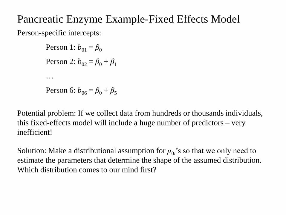
Person-specific intercepts:

Person 1: b01 = β0

Person 2: b02 = β0 + β1

…

Person 6: b06 = β0 + β5

Potential problem: If we collect data from hundreds or thousands individuals,

this fixed-effects model will include a huge number of predictors – very

inefficient!

Solution: Make a distributional assumption for μ0i’s so that we only need to

estimate the parameters that determine the shape of the assumed distribution.

Which distribution comes to our mind first?

Introduce Subject Random Effects

Suppose we are mainly interested in the relationship between fat measure and

pilltype, and less interested in the person-specific averages.

As before, let Yij be the excreted fat for the jth pilltype administered to the ith

patient. But now we split the error term into a subject specific effect bi and a

residual error effect 𝑒𝑖𝑗∗ .

𝑌𝑖𝑗 = 𝜇𝑗 + 𝑒𝑖𝑗 = 𝜇𝑗 + 𝑏𝑖 + 𝑒𝑖𝑗∗

We now assume 𝑏𝑖~𝑖𝑖𝑑𝑁 0, 𝜎𝑠𝑢𝑏𝑗𝑒𝑐𝑡2 and 𝑒𝑖𝑗

∗ ~𝑖𝑖𝑑𝑁 0, 𝜎2 .

Treating bi as a random effect (rather than a fixed term) is interpreted as the

individuals in our study being some random sample from a larger population of

subjects which we wish to make inference. We would treat subjects as fixed

effects (i.e. as in the previous slide), if we were interested in making inference

about the 6 specific people.

Fitting Random Effects Model – SAS (1) proc mixed data = long1;

class pilltype personid;

model fat = pilltype / solution;

random intercept / subject = personid; ** person specific random effects;


run;

Dependent Variable fat

Covariance Structure Variance Components

Subject Effect personid level 2 unit identifier

Estimation Method REML estimation method (alternative: MLE)

Residual Variance Method Profile

Fixed Effects SE Method Model-Based

Degrees of Freedom Method Containment

Dimensions

Covariance Parameters 2

Columns in X 5 number of fixed effects

Columns in Z Per Subject 1 1 random effect (random intercept)

Subjects 6

Max Obs Per Subject 4

Covariance Parameter Estimates

Cov Parm Subject Estimate

Intercept personid 252.67 estimated 𝜎𝑠𝑢𝑏𝑗𝑒𝑐𝑡2

Residual 107.00 estimated 𝜎2

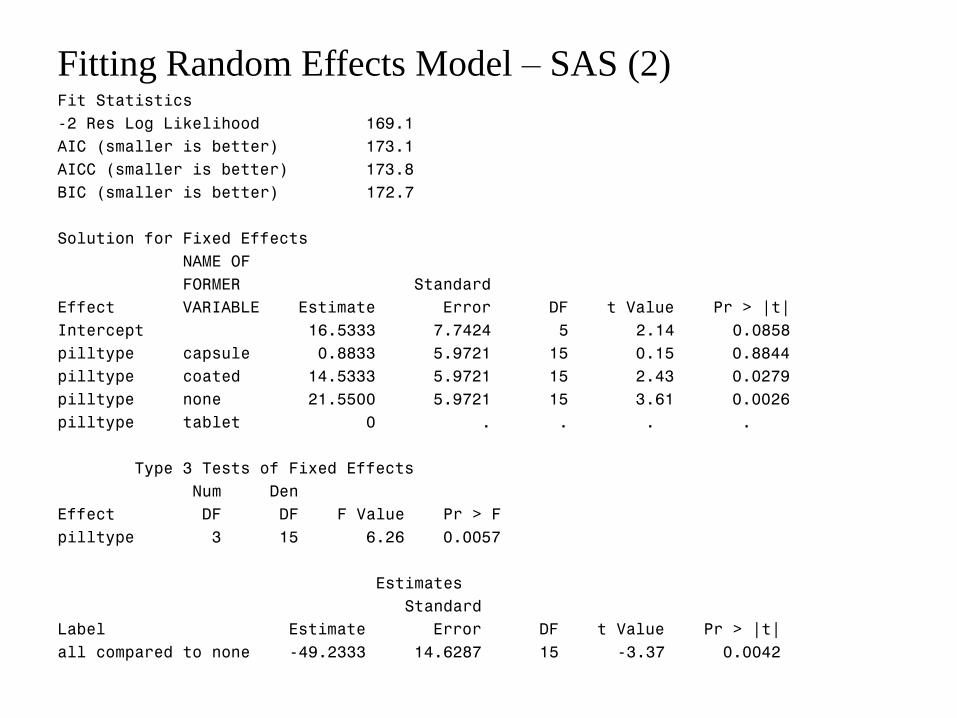
Fitting Random Effects Model – SAS (2) Fit Statistics

-2 Res Log Likelihood 169.1

AIC (smaller is better) 173.1

AICC (smaller is better) 173.8

BIC (smaller is better) 172.7

Solution for Fixed Effects

NAME OF

FORMER Standard

Effect VARIABLE Estimate Error DF t Value Pr > |t|

Intercept 16.5333 7.7424 5 2.14 0.0858

pilltype capsule 0.8833 5.9721 15 0.15 0.8844

pilltype coated 14.5333 5.9721 15 2.43 0.0279

pilltype none 21.5500 5.9721 15 3.61 0.0026

pilltype tablet 0 . . . .

Type 3 Tests of Fixed Effects

Num Den

Effect DF DF F Value Pr > F

pilltype 3 15 6.26 0.0057

Estimates

Standard

Label Estimate Error DF t Value Pr > |t|

all compared to none -49.2333 14.6287 15 -3.37 0.0042

Fitting Random Effects Model – SAS (3)

Notice the error degrees of freedom are now 15 rather than 20 as in WRONG

ANALYSIS, why?

Also notice that the previous error variance of 359.6 has been split into subject-

to-subject variance 252.67 plus true error variance 107. Notice that because the

error variance is smaller, the p-values for pilltype are more significant. (more

details in next slides)

Also notice that the point estimates for each pilltype is the same as those in

fixed-effects model.

Fitting Random Effects Model – Stata . xtmixed fat ib(last).pilltype || personid:, variance reml

Mixed-effects REML regression Number of obs = 24

Group variable: personid Number of groups = 6

Obs per group: min = 4

avg = 4.0

max = 4

Wald chi2(3) = 18.77

Log restricted-likelihood = -84.555945 Prob > chi2 = 0.0003

------------------------------------------------------------------------------

fat | Coef. Std. Err. z P>|z| [95% Conf. Interval]

-------------+----------------------------------------------------------------

pilltype |

1 | .8833336 5.972126 0.15 0.882 -10.82182 12.58849

2 | 14.53333 5.972126 2.43 0.015 2.828181 26.23848

3 | 21.55 5.972126 3.61 0.000 9.844849 33.25515

|

_cons | 16.53333 7.742398 2.14 0.033 1.358512 31.70815

------------------------------------------------------------------------------

------------------------------------------------------------------------------

Random-effects Parameters | Estimate Std. Err. [95% Conf. Interval]

-----------------------------+------------------------------------------------

personid: Identity |

var(_cons) | 252.6695 176.99 64.01811 997.247

-----------------------------+------------------------------------------------

var(Residual) | 106.9989 39.07045 52.30755 218.8739

------------------------------------------------------------------------------

LR test vs. linear regression: chibar2(01) = 12.52 Prob >= chibar2 = 0.0002

Fitting Random Effects Model – Stata . test 1.pilltype 2.pilltype 3.pilltype // joint test for pilltype effect

( 1) [fat]1.pilltype = 0



chi2( 3) = 18.77

Prob > chi2 = 0.0003

. lincom 1.pilltype+2.pilltype-3*3.pilltype // all compared to none

( 1) [fat]1.pilltype + [fat]2.pilltype - 3*[fat]3.pilltype = 0

------------------------------------------------------------------------------

fat | Coef. Std. Err. z P>|z| [95% Conf. Interval]

-------------+----------------------------------------------------------------

(1) | -49.23334 14.62866 -3.37 0.001 -77.90498 -20.56169

------------------------------------------------------------------------------

. contrast {pilltype 1 1 -3 1} // available in Stata 12

Contrasts of marginal linear predictions

Margins : asbalanced

------------------------------------------------

| df chi2 P>chi2

-------------+----------------------------------

fat |

pilltype | 1 11.33 0.0008

------------------------------------------------

--------------------------------------------------------------

| Contrast Std. Err. [95% Conf. Interval]

-------------+------------------------------------------------

fat |

pilltype |

(1) | -49.23334 14.62866 -77.90498 -20.56169

--------------------------------------------------------------

Fitting Random Effects Model

The uncertainty about how treatment will work NOW can be estimated by

considering the deviation between the observed values for a person and the

expected value for that person. The variance of the 𝑒𝑖𝑗∗ in the new model is the

variability AFTER accounting for person to person variability.

*. Why the fitted

lines are parallel?


This variability is calculated within each person and then (averaged) across

individuals. Plot below shows the data and expected values for Person 5 and

Person 3. The variance is 107. This is MUCH SMALLER than that in WRONG

ANALYSIS. Hence tests for treatment differences are more powerful since the

treatment differences (i.e. mean change in fat across different treatments) are

compared to an uncertainty of 107 rather than 359.


Notice that the standard errors are much smaller than those in WRONG

ANALYSIS, because here they are constructed using 107 rather than 359 as the

estimate for σ2. Recall that the estimated standard errors are σ2(X’X)-1.

Predict Random Effects

We can predict (not estimate) the random intercepts for each person by adding

solution option in the random statement.

...; random intercept / subject = personid solution; run;

Solution for Random Effects

Std Err

Effect personid Estimate Pred DF t Value Pr > |t|

Intercept 1 -8.0254 7.8911 15 -1.02 0.3253

Intercept 2 -0.1356 7.8911 15 -0.02 0.9865

Intercept 3 -10.2182 7.8911 15 -1.29 0.2149

Intercept 4 -17.7914 7.8911 15 -2.25 0.0395

Intercept 5 19.2835 7.8911 15 2.44 0.0274

Intercept 6 16.8872 7.8911 15 2.14 0.0492

In Stata, use: . predict varname, reffects

Predict Random Effects

To predict bi, we can use:

𝑏𝑖 = 𝐸 𝑏𝑖|𝑌𝑖

which is called best linear unbiased prediction (BLUP). In the random intercept

model,

𝑏𝑖 = 𝐸 𝑏𝑖|𝑌𝑖 =

𝑛𝑖 𝜎𝑠𝑢𝑏𝑗𝑒𝑐𝑡2

𝑛𝑖 𝜎𝑠𝑢𝑏𝑗𝑒𝑐𝑡2 + 𝜎2

𝑌𝑖 − 𝜇

which is known as “shrinkage estimator” – weighted derivation of 𝑌𝑖 and 𝜇.

Define: 𝜇𝑖 = 𝐸 𝑌𝑖𝑗|𝑏𝑖 = 𝜇 + 𝑏𝑖.

When 𝜎𝑠𝑢𝑏𝑗𝑒𝑐𝑡2 → ∞, 𝜇𝑖 = 𝑌𝑖

;

𝜎2→ ∞, 𝜇𝑖 = 𝜇 .

Random Effects vs Fixed Effects

The random effects are “shrunk”, i.e. smaller (closer to zero) than the fixed

effects estimates. In this example with balanced data (i.e. same number of

observations within subject), the standard errors are same using two methods.

Using fixed subject effect, we cannot then test for subject level covariates since

completely confounded

Correlation Within Subjects

The subject specific random effects in the model induce a correlation between

observation within a person.

This correlation is known as the “intraclass correlation” sometimes denoted ρI.

Including Subject Specific Covariates

Recall we know the gender of each patient. So we may expect that part of the

reason there is variability in the bi in our model is that there are differences due

to gender.

𝑌𝑖𝑗 = 𝜇𝑗 + 𝑏𝑖 + 𝑒𝑖𝑗 -- LEVEL 1

𝑏𝑖 = 𝛽0 + 𝛽1𝑓𝑒𝑚𝑎𝑙𝑒 + 𝛿𝑖 -- LEVEL 2

where we assume 𝛿𝑖~𝑖𝑖𝑑𝑁 0, 𝜎𝑠𝑢𝑏𝑗𝑒𝑐𝑡2 and 𝑒𝑖𝑗~𝑖𝑖𝑑𝑁 0, 𝜎2 .

NOTICE that this 2-level model can be collapsed into a single equation:

𝑌𝑖𝑗 = 𝜇𝑗 + 𝛽0 + 𝛽1𝑓𝑒𝑚𝑎𝑙𝑒 + 𝛿𝑖 + 𝑒𝑖𝑗

where the 𝛽0 + 𝛽1𝑓𝑒𝑚𝑎𝑙𝑒 can get folded into the regular fixed regression part

of the model, and now 𝛿𝑖 represents the subject to subject variability found

after accounting for the fixed differences between males and females.

So the Level 2 covariates can be treated simply as regular fixed covariates.

Pancreas enzyme example - including gender proc mixed data = long1;

class pilltype personid gender;

model fat = pilltype gender/solution ddfm=bw;

random intercept / subject = personid solution;


run;


Cov Parm Subject Estimate

Intercept personid 57.8536

Residual 107.00

Type 3 Tests of Fixed Effects

Num Den

Effect DF DF F Value Pr > F

pilltype 3 15 6.26 0.0057

gender 1 4 12.51 0.0241

Estimates

Standard

Label Estimate Error DF t Value Pr > |t|

all compared to none -49.2333 14.6287 15 -3.37 0.0042

Pancreas enzyme example - including gender Solution for Fixed Effects

NAME OF

FORMER Standard

Effect VARIABLE gender Estimate Error DF t Value Pr > |t|

Intercept 3.2500 6.4479 4 0.50 0.6407

pilltype capsule 0.8833 5.9721 15 0.15 0.8844

pilltype coated 14.5333 5.9721 15 2.43 0.0279

pilltype none 21.5500 5.9721 15 3.61 0.0026

pilltype tablet 0 . . . .

gender F 26.5667 7.5101 4 3.54 0.0241

gender M 0 . . . .

Now the person level variance has decreased dramatically to 57.85 from 252.67

in previous model. But the Residual variance is unchanged.

We can say that (252.67 − 57.85)/252.67 = 77% of the overall subject-to-

subject variability is explained by differences due to gender. Notice including

gender has no effect on the within subject effect of pilltype. Generally there can

be changes in the within subject effect when between subject covariates are

included.

Denominator degrees of freedom

• For testing within subject covariates: 𝑛𝑖 − 1 −𝑁𝑖=1 (# within subject

covariates but don’t count intercept)

• For testing between subject covariates: N - (# of between subject covariates

+ intercept)

where N is the number of groups (i.e. clusters) and 𝑛𝑖 is the number of

observations within group i.

For the pancreatic enzyme example, N = 6, 𝑛𝑖 = 4, i = 1. . . 6, so we have:

• For testing within subject covariates (pilltype), d.f. = [ 4 − 1 6𝑖=1 ] −3 = 18

− 3 = 15

• For testing between subject covariates (gender), d.f. = 6 − (1 + 1) = 4

NOTE: IF the denominator degrees of freedom are larger than 25 then (similar

to the t test which is well approximated by normal for larger n), it doesn’t really

matter exactly what they are since the F-distribution is well approximated by

the Chi-square distribution for larger n.

NOTE: Stata uses the Chi-square test instead of F-test, in which the d.f. is

simply the number of parameters being tested.

Outcomes at the individual level, covariates at the

cluster level

Consider the following data representing age and gender standardized weight

measurements (called indwt) on each member of 100 families. Family size

ranges from 2 to 7 people - the NA’s are just place holders for families with less

than 7 members. The SES variable represents high (1) and low (0) social

economic status.

What is the association between SES and standardized weight?

Different Approaches

• Ignore the fact that people are sampled in clusters of families. In total there

are 416 individuals who we have weights. Regress individual weights on

SES. - Will tend to lead to overly optimistic results (standard errors too

small)

• Create family level mean weights. There are 100 families. Regress mean

family weight on SES. - If family sizes are about equal (gives equal weight

to each mean) -- not a bad method for examining group level covariates but

does not allow for individual level covariates

• Randomly pick one member of each family so then we have 100

independent individuals and then regress individual weight (of randomly

chosen family member) on SES. - Throws away information (standard

errors too large, less power)

• Use a multilevel model that utilizes all 416 individuals measurements while

partitioning variance due to family differences not explained by SES. –

Correct compromise between methods 1 and 2 above, correctly tests subject

level covariates while also allowing the possibility of individual level

covariates.

Results of Different Approaches: Family Weight Data

Data were simulated under a few different scenarios which varied by how much

of the family level variability was explained by SES. Overall in each scenario,

the percent of total variability was fixed in the weight measurements that is

coming from the family level clusters to be 0.80. In other words, 80% of

variability in weight can be explained by family differences, while only .01,

.02, or .05 of those differences can be explained by family SES.

Notice the similarity between betaRE and betaagg. Notice that betaiid is

rejecting highly in all cases (standard errors are too small) and that

betaChoose1 is slightly conservative (larger standard errors), but not much.

Random Intercepts

In fat enzyme example:

𝑌𝑖𝑗 = 𝛽0𝑖 + 𝛽1 ∗ 𝑡𝑟𝑡 + 𝑒𝑖𝑗

𝛽0𝑖 = 𝛽0 + 𝑏𝑖

𝛽0𝑖 represent person specific intercept (based on trt reference of “tablet”, the

intercept is the person specific estimate for trt of type “tablet”). We used the

within person variability of 𝑒𝑖𝑗 to test for treatment effect.

In family SES related to weight example:

𝑌𝑖𝑗 = 𝛽0𝑖 + 𝑒𝑖𝑗

𝛽0𝑖 = 𝛽0 + 𝛽1 ∗ 𝑆𝐸𝑆 + 𝑏𝑖

𝛽0𝑖 represents family specific average weight. Variance of bi represents

deviation of family specific average weight from that expected based on their

SES. We used the between person variability of bi to test for SES effect.

Random Intercepts and Random Slopes

We have focused so far on taking into account clustering by including a random

intercept into the model. It may also be of interest to examine whether the way

that individual level covariates effect the outcome vary by cluster as well. This

implies that slopes vary by cluster.

We will consider a now classic dataset from the 1982 ”High School and

Beyond” survey on Math Achievement of 7185 students from 160 schools. The

data was used in Bryk and Raudenbush’s first edition 1992 text Hierarchal

Linear Models

• A step-by-step analysis of the data using SAS was done by Judith Singer in

Journal of Educational and Behavioral Statistics and also can be found at

http://www.ats.ucla.edu/stat/sas/seminars/sas_mlm/mlm_sas_seminar.htm

• A step-by-step analysis of the data using R was done by John Fox as an

appendix to his text An R and S-plus Companion to Applied Regression

We want to examine whether the way a child’s own SES (cses) is related to

his/her math achievement (mathach) varies by what school they are in. That is,

can “contextual factors” (i.e. school level variability) moderate the relationship

between SES and achievement.

Random Slope: Compare to Interaction Model

• Suppose we suspect the relationship between mathach and cses varies by

school:

– Our level 1 (student level) equation becomes:

mathachij = β0i + β1i*csesij + eij

note the subscript change from β1 to β1i for SES effect.

– On level 2, we try to explain the variation of slopes of cses by school’s

SES (meanses) and sector status (sector).

• Fixed effects: We can use a deterministic model,

β1i = β10 + β11*meanses + β12*sector

i.e., meanses and sector can fully explain the variation of slopes.

When we plug level 2 equation back to level 1, we get a fixed-effects

model with cses, meanses*cses, and sector*cses as the predictors.

We could also estimate school-specific slopes, which is equivalent to

add school*cses interactions. But there will be too many predictors,

since there are 160 levels for school.

Random Slope: Compare to Interaction Model (2)

• Random effects: If we think meanses and sector cannot fully

explain the variation of slopes, we can include a random error term

to level 2 equation for the unaccounted-for variation.

β1i = β10 + β11*meanses + β12*sector + b1i

where b1i ~ N(0, σ2cses).

Plug level 2 equation back to level 1, we will get fixed effects for

cses, meanses*cses, and sector*cses, and random slope term b1i *cses.

Random Intercept and Slope and Covariates at Both Levels

𝑌𝑖𝑗 = 𝛽0𝑖 + 𝛽1𝑖𝑋𝑖𝑗 + 𝑒𝑖𝑗

𝛽0𝑖 = 𝛼00 + 𝛼01𝑊𝑖 + 𝛿0𝑖

𝛽1𝑖 = 𝛼10 + 𝛼11𝑊𝑖 + 𝛿1𝑖

where 𝑒𝑖𝑗~𝑁 0, 𝜎2 and 𝛿0𝑖

𝛿1𝑖~𝑁

00

,𝜏00 𝜏10

𝜏10 𝜏11

Xij represents a Level 1 covariate, e.g. child specific social economic status (in

Math Achievement example). The Level 1 equation assumes that in each

cluster i that there is a linear relationship between the covariate and the

outcome and this relationship is allowed to be different across clusters.

The Level 2 equations and the distribution of 𝛿0𝑖 and 𝛿1𝑖 provide information

about how the intercept and slope of the Level 1 equation vary across clusters,

e.g. the school’s mean SES level as well as the type of school (private or

public) may influence the intercept Math Achievement (𝛽0𝑖) and may influence

the way that a child’s own SES relates to Math Achievement (𝛽1𝑖).

Level 2 Covariates for Slopes Lead to Interactions

When we plug in the Level 2 equations into the Level 1 equation, we get

𝑌𝑖𝑗 = 𝛼00 + 𝛼01𝑊𝑖 + 𝛿0𝑖 + 𝛼10 + 𝛼11𝑊𝑖 + 𝛿1𝑖 𝑋𝑖𝑗 + 𝑒𝑖𝑗

= 𝛼00 + 𝛿0𝑖 + 𝛼10 + 𝛿1𝑖 𝑋𝑖𝑗 + 𝛼01𝑊𝑖 + 𝛼11𝑊𝑖 ∗ 𝑋𝑖𝑗 +𝑒𝑖𝑗

Notice, if the coefficient for the interaction term 𝛼11 is not significant this

implies that the cluster level covariate Wi does not help explain differential

slope relationship between Xij and the outcome (but it does not exclude other

source of variability among the slopes).

Examining Random Intercepts and Slopes

Math achievement example: from John Fox’s appendix to An R and S-PLUS

Companion to Applied Regression

Trellis display of math achievement by socio-economic status for 20 randomly

selected Catholic schools. The broken lines give linear least-squares fits, the

solid lines local-regression fits.




Trellis display of math achievement by socio-economic status for 20 randomly

selected Public schools. The broken lines give linear least-squares fits, the

solid lines local-regression fits.




Boxplots of intercepts and slopes for the SEPARATE regressions of math

achievement on SES in Catholic and public schools. It appears SECTOR

explains some variability in the intercepts and in the slopes, in what way?


Math achievement example: Results including both SECTOR and MEANSES

as level 2 covariates

Testing Whether Random Coefficients Are Needed

• Testing whether a random coefficient should be included in a multilevel

model involves the test of whether the variance of that random coefficient

is equal to 0. This is problematic because the null hypothesis lies on the

boundary of the parameter space.

• A Wald test and the likelihood ratio statistics can be considered but the

problem is technically they don’t have nominal Type 1 errors.

• There is a substantial literature about approximate tests for the variance

components, e.g. using a mixture of a chi-square as a reference distribution

with k and k+1 degrees of freedom (where k is the number of variance

components being tested). These methods do not appear to implemented

yet in existing software.

• Recommendation is to use the AIC or BIC criteria to decide by comparing

models with and without the random coefficients.

Random Intercept and Slope and Covariates at Both Levels

𝑌𝑖𝑗 = 𝛽0𝑖 + 𝛽1𝑖𝑋𝑖𝑗 + 𝑒𝑖𝑗

𝛽0𝑖 = 𝛼00 + 𝛼01𝑊𝑖 + 𝛿0𝑖

𝛽1𝑖 = 𝛼10 + 𝛼11𝑊𝑖 + 𝛿1𝑖

where 𝑒𝑖𝑗~𝑁 0, 𝜎2 and 𝛿0𝑖

𝛿1𝑖~𝑁

00

,𝜏00 𝜏10

𝜏10 𝜏11

Specifically for the example we’ve seen, Yij represents Math Achievement,

where i subscripts schools and j subscripts kids within schools. Xij would be

kid level SES, Wi could be an indicator of whether the school is catholic or

public.

In general Xij could by p-dimensional, and so β1i would also be p-dimensional

with potential for random variation associated with each covariate.

Furthermore Wi could be q-dimensional.

General Formulation for the Mixed Effects Model

Let Yi be the response vector for each level 2 unit i (e.g. either each school in

Math Achievment example or family in weight-ses example or individual in fat

enzyme example ) which will have length ni (e.g. where ni is the number of

kids in school i or the number of persons in family or 4 treatments in enzyme

example). Then we can write in general matrix notation...

General Formulation for the Mixed Effects Model

Note that across i the vectors of observations Yi are i.i.d. (e.g. schools are

independent or mice are independent from one another), implicitly this is

because we assume bi are ei are i.i.d. across i. Further, since we assume a linear

link between Yi and the predictors, then the normality assumption on bi are ei

imply that

𝒀𝑖~𝑖. 𝑖. 𝑑 𝑁 𝑿𝑖𝛽, 𝒁𝑖𝑮𝒁𝑖′ + 𝑹𝑖

where G = Var(bi) and Ri is a matrix specifying the covariance of the ei which

will typically be a function of a few parameters e.g. σ2 and ρ.

Estimation by Maximum Likelihood Let 𝑉𝑎𝑟 𝒀𝑖 = 𝑽𝑖 = 𝒁𝑖𝑮𝒁𝑖

′ + 𝑹𝑖. Let Y be the vector which stacks all the

𝑛𝑖𝑁𝑖=1 observations, similarly let X be the matrix which stacks all the

covariates Xi and finally let V be the block diagonal matrix with matrices Vi

on the diagonal, similarly R is the block diagonal matrix of Ri. Then the log-

likelihood is a function of the multivariate normal distribution, i.e.

which can be optimized to find the MLE’s of β, G, and R.

This looks similar to the log likelihood for the general linear model except here

V is more complicated and has several parameters within it that need to be

estimated.

Note, in the general linear model from before, we did NOT have G or Zi at all

and R = σ2 I.

Estimation by Maximum Likelihood OLS (ordinary least squares) can be shown to be the same as maximum likelihood for normally distributed data for the general linear model. Here notice the form 𝑌 − 𝑋𝛽 ′𝑉−1 𝑌 − 𝑋𝛽 in the likelihood. This has the form of Generalized Least

Squares (GLS) and represents the quantity we want to minimize. However, to do this requires V to be known and therefore G and R to be known. One approach is to use an estimated 𝑉 and plug this in, hence the task is to obtain reasonable estimates for G and R.

In principle the likelihood is straightforward to maximize the likelihood but problems arise in estimating the variance parameters G and R. There are different numerical algorithms which can be used to find the optimal G and R, in smaller samples they may give different results.

It can happen that ML finds the “best fitting” variance parameters to be negative. Since a negative variance is not a possible value, the reported estimate is taken to be zero.

Also, since it is well known that ML variance estimates are biased (since they use n rather than n-1 as denominators), a commonly preferred technique (and the default in SAS/R, but not STATA) is to use REML which stands for restricted (or residual) maximum likelihood. Essentially REML uses an unbiased method for estimating the variance components.

Mixed Effect Models for Non-normal Responses

A generalized linear model which incorporates random effects is called a

“generalized linear mixed model”.

As long as the link is linear, it is feasible to obtain estimates for the mixed

effect model 𝒀𝑖 = 𝑿𝑖𝛽 + 𝒁𝑖𝑏𝑖 + 𝑒𝑖. When our outcome data is not modeled

well with a linear link to the mean structure, e.g. binary data with a logit link,

or Poisson data with a log link, then estimation becomes much more difficult

using Maximum likelihood.

The reason is that the corresponding likelihood

has an integral in it that does not lend itself to straightforward maximization.

Estimation for Generalized Linear Mixed Models

A variety of approaches are available (still an active area of research) to

approximate this likelihood using theoretical and numerical methods.

• In SAS, PROC NLMIXED/ In STATA: xtmelogit; xtmepoisson; gllamm

(user-written package) in STATA / In R the nlme() function can be used to

maximize the likelihood for a generalized linear mixed model, also

Bayesian methods are commonly implemented for this model. Though

theoretically maximizing the likelihood is the best approach, it is common

to run into computational problems with these numerical methods.

• Another approach, which may be referred to as Pseudo-likelihood

(Wolfinger, R. and O’Connell, M. (1993) Generalized linear mixed models:

a pseudo-likelihood approach. Journal of Statistical Computation and

Simulation 48, 233-243) which is implemented by Proc GLIMMIX

(formerly the GLIMMIX macro in SAS) and approximates the nonlinear

likelihood with a linear form and iteratively improves the estimates for G

and R. It can also be implemented in R using glmmPQL().

• Completely avoid the likelihood and instead focus on Generalized

Estimating Equations (GEE).

Generalized Estimating Equations Consider again 𝒀𝑖 which represents the vector of observations in the i

th cluster.

Let E(𝒀𝑖) = μi which is linked to the linear predictor such that g(μi) = Xiβ. Let Var(𝒀𝑖) ≡ Var(𝒀𝑖; β, α) where α represents parameters that model the correlation structure within individuals.

Parameters β are then estimated by solving the following score equation

𝜕𝜇𝑖

𝜕𝛽

′

𝑉𝑎𝑟 𝑌𝑖−1 𝑌𝑖 − 𝜇𝑖 = 0

𝑁

𝑖=1

• The key point which makes this method feasible and robust is that we don’t need to know Var(𝒀𝑖), the estimates for β are consistent even if Var(𝒀𝑖) is misspecified.

• In GEE we use what is called the “working correlation matrix” as the best guess to the structure of Var(𝒀𝑖).

• This lack of focus on the Var(𝒀𝑖) is the key difference between random effects modeling and using GEE. With GEE, the focus is entirely on getting good estimates of β and their standard errors. We will not obtain estimates of person level variability or be able to say that some covariate explained X% of the between person variability.

Standard Errors for GEE

There are two types of standard errors available for GEE:

1. Model Based taken from the Co𝑣 𝛽 = 𝐼0−1 where

𝐼0 = 𝜕𝜇𝑖

𝜕𝛽

′𝑉𝑖

−1𝑁𝑖=1

𝜕𝜇𝑖

𝜕𝛽

2. Empirical or robust or “sandwich formula” which uses Co𝑣 𝛽 = 𝐼0−1𝐼1𝐼0

−1

where 𝐼1 = 𝜕𝜇𝑖

𝜕𝛽

′𝑉𝑖

−1𝐶𝑜𝑣 𝑌𝑖 𝑉𝑖−1𝑁

𝑖=1𝜕𝜇𝑖

𝜕𝛽 where 𝐶𝑜𝑣 𝑌𝑖 is replaced by

the sum of squared residuals, i.e. 𝑌𝑖 − 𝜇𝑖 𝛽 𝑌𝑖 − 𝜇𝑖 𝛽 ′

The Model Based standard errors will only be correct when the correlation

structure for Vi is specified correctly. But, the robust “sandwich” estimator can

perform poorly in data with small samples. The “sandwich” estimator is

consistent for the standard errors even when the correlations are specified

incorrectly, but this property doesn’t kick-in unless the N is large especially

compared to the ni (i.e. more clusters not more measurements within cluster)

Both SAS and R use the robust standard errors by default. Stata uses the model

based by default.

Implementing GEE in SAS, R, and Stata

In SAS: use Proc GENMOD with a Repeated statement.

In R: use function gee()

In STATA: use xtgee or xtreg with the pa “population average” option

Need to specify the “working correlation matrix”, that is, a covariance

structure that mimics the likely covariance structure in the data. Common

structures are: Compound symmetry or Exchangeable, Autoregressive,

Unstructured, and Independent.

Pros and Cons of GEE compared to Generalized linear

Mixed effect modeling (GLMM)

• GEE: Only one level of clustering, GLMM: multiple levels

• GEE: Not designed for inference about the covariance of random part,

GLMM: Can do inference on covariance of error structure (random part)

• GEE: Does not give predicted values for each cluster, GLMM: can obtain a

predicted value separate for each cluster.

• GEE: Computationally straightforward and fast, GLMM: Computationally

hard and slow

• GEE: Consistent estimates of fixed effect parameters, GLMM: Consistent

estimates of fixed effects parameters and most efficient if random effects

covariance structure is correct.

• GEE: Assumes missing data is MCAR, GLMM: Assumes missing data is

MAR

• GEE: fits marginal model, GLMM: fits conditional model

Marginal versus Conditional Models

There are two main ways to build in correlation in a statistical model:

• Marginal: Assume a model, e.g. logistic, that holds averaged over all the

clusters (sometimes called population averaged). Coefficients have the

interpretation as the average change in the response (over the entire

population) for a unit change in the predictor.

• Conditional: Assume a model specific to each cluster (sometimes called

subject specific). If you want to know about the population, average it over

all the clusters. Coefficients have the interpretation as the change in the

response for each cluster in the population.

NOTE: when the outcome-predictor relationship is linear, these are equivalent.

That is, the average of the individual’s coefficients is the same as the overall

population (or marginal) coefficient. When the relationship is non-linear, e.g.

logit, they are NOT the same. See example taken from VGSM text Section 8.5.

Marginal versus Conditional Models Hypothetical example from VGSM text Section 8.5...

Suppose we are modeling the chance that a patient will be able to withstand a course of chemotherapy without serious adverse reactions. Patients have very different tolerances for chemotherapy, so the subject specific curves are quite different (See plots on next pages)...

For further reading of the differences between marginal (GEE) and conditional models (GLMM) see:

Carriere I and Bouyer J (2002) Choosing marginal or random-effects models for longitudinal binary responses: application to self-reported disability among older persons, BMC Medical research Methodology, 2:15.

Burton, P., Gurrin, L., Sly, P. Tutorial in Biostatistics: Extending the Simple Linear Regression Model to Account for Correlated Responses: An Introduction to Generalized Estimating Equations and Multi-Level Modelling” Statistics in Medicine 17, 1261-1291 (1998).

Anath CV, Platt RW, Savitz DA (2005) Regression Models for clustered binary responses: implications of ignoring the intracluster correlation in an analysis of perinatal mortality in twin gestations. Annals of Epidemiology, 15(4), 293-301.

Hubbard AE, Ahern J, Fleischer NL et al. (2010) To GEE or Not to GEE Comparing Population Average and Mixed Models for Estimating the Associations Between Neighborhood Risk Factors and Health. Epidemiology, Volume 21, Number 4, July 2010

Non-Linear Link: Georgia Birthweight Example

Georgia Birthweight data: birthweights of first-born and last-born infants from

mothers (each of whom had five children) from vital statistics in Georgia.

(VGSM Chapter 8.3.2)

Research question: How the low birthweight status (<3,000g) of babies

changes by birth order (first to fifth) and whether this difference depends on

the age of the woman when she had her first-born.

Georgia Birthweight Example: independent correlation . xtgee lowbrth birthord initage, i(momid) corr(ind) family(binomial) link(logit) ef

GEE population-averaged model Number of obs = 1000

Group variable: momid Number of groups = 200

Link: logit Obs per group: min = 5

Family: binomial avg = 5.0

Correlation: independent max = 5

Wald chi2(2) = 18.13

Scale parameter: 1 Prob > chi2 = 0.0001

Pearson chi2(1000): 1003.09 Deviance = 1299.35

Dispersion (Pearson): 1.003089 Dispersion = 1.299354

------------------------------------------------------------------------------

lowbrth | Odds Ratio Std. Err. z P>|z| [95% Conf. Interval]

-------------+----------------------------------------------------------------

birthord | .9204561 .0430753 -1.77 0.077 .8397861 1.008875

initage | .9155828 .0207316 -3.89 0.000 .875838 .9571313

_cons | 3.505028 1.477288 2.98 0.003 1.534368 8.006694

------------------------------------------------------------------------------

This is equivalent to:

. glm lowbrth birthord initage, family(binomial) link(logit) ef

Georgia Birthweight Example: exchangeable correlation . xtgee lowbrth birthord initage, i(momid) corr(exch) family(binomial) link(logit) ef

GEE population-averaged model Number of obs = 1000


Link: logit Obs per group: min = 5

Family: binomial avg = 5.0

Correlation: exchangeable max = 5

Wald chi2(2) = 11.30

Scale parameter: 1 Prob > chi2 = 0.0035

------------------------------------------------------------------------------


-------------+----------------------------------------------------------------

birthord | .9204098 .0359157 -2.13 0.034 .8526408 .9935651

initage | .9148199 .0308985 -2.64 0.008 .856221 .9774293

_cons | 3.553325 2.144814 2.10 0.036 1.088537 11.59917

------------------------------------------------------------------------------

Robust standard errors: . xtgee lowbrth birthord initage, … vce(robust)

------------------------------------------------------------------------------

| Semirobust


-------------+----------------------------------------------------------------

birthord | .9204098 .03542 -2.16 0.031 .8535413 .9925168

initage | .9148199 .0312663 -2.60 0.009 .8555464 .9781999

_cons | 3.553325 2.167263 2.08 0.038 1.075142 11.74368

------------------------------------------------------------------------------

Georgia Birthweight Example: exchangeable correlation proc genmod data=bwt descending;

class momid;

model lowbrth=birthord initage / dist = binomial link = logit type3;

repeated subject = momid /type = cs modelse;

estimate "OR(birthord)" birthord 1/exp;

estimate "OR(initage)" initage 1/exp;

run;

Exchangeable Working

Correlation

Correlation 0.3049933764 In Stata, use –estat wcor- after –xtgee- to obtain this estimate

GEE Fit Criteria

QIC 1309.6471 similar to AIC/BIC in LMM. In stata, download –qic- package

QICu 1305.3556

Analysis Of GEE Parameter Estimates

Empirical Standard Error Estimates

Standard 95% Confidence

Parameter Estimate Error Limits Z Pr > |Z|

Intercept 1.2679 0.6084 0.0754 2.4603 2.08 0.0372

birthord -0.0829 0.0384 -0.1582 -0.0077 -2.16 0.0307

initage -0.0890 0.0341 -0.1558 -0.0222 -2.61 0.0090

Analysis Of GEE Parameter Estimates

Model-Based Standard Error Estimates

Standard 95% Confidence

Parameter Estimate Error Limits Z Pr > |Z|

Intercept 1.2679 0.6034 0.0853 2.4504 2.10 0.0356

birthord -0.0829 0.0390 -0.1594 -0.0064 -2.12 0.0336

initage -0.0890 0.0338 -0.1552 -0.0229 -2.64 0.0084

Georgia Birthweight Example: GLMM proc glimmix data=bwt;

class momid;

model lowbrth(descending)=birthord initage / dist = binomial link = logit solution;

random intercept / subject = momid;

estimate "OR(birthord)" birthord 1/exp;

estimate "OR(initage)" initage 1/exp;

run;

The GLIMMIX Procedure


Standard

Cov Parm Subject Estimate Error

Intercept momid 1.5042 0.2755

Solutions for Fixed Effects

Standard

Effect Estimate Error DF t Value Pr > |t|

Intercept 1.4250 0.6700 198 2.13 0.0347

birthord -0.09961 0.05132 799 -1.94 0.0526

initage -0.1002 0.03684 799 -2.72 0.0067

Estimates

Standard Exponentiated

Label Estimate Error DF t Value Pr > |t| Estimate

OR(birthord) -0.09961 0.05132 799 -1.94 0.0526 0.9052

OR(initage) -0.1002 0.03684 799 -2.72 0.0067 0.9047

Georgia Birthweight Example: GLMM . xtmelogit lowbrth birthord initage || momid:, or var

Mixed-effects logistic regression Number of obs = 1000


Obs per group: min = 5

avg = 5.0

max = 5

Integration points = 7 Wald chi2(2) = 11.85

Log likelihood = -588.07113 Prob > chi2 = 0.0027

------------------------------------------------------------------------------


-------------+----------------------------------------------------------------

birthord | .8872745 .0500702 -2.12 0.034 .7943711 .9910432

initage | .8808974 .0406081 -2.75 0.006 .8047967 .9641941

_cons | 6.009049 4.991562 2.16 0.031 1.1796 30.61095

------------------------------------------------------------------------------

------------------------------------------------------------------------------

Random-effects Parameters | Estimate Std. Err. [95% Conf. Interval]

-----------------------------+------------------------------------------------

momid: Identity |

var(_cons) | 2.58756 .5393782 1.719718 3.893354

------------------------------------------------------------------------------

LR test vs. logistic regression: chibar2(01) = 123.21 Prob>=chibar2 = 0.0000

Note: Stata and SAS use different methods (MLE vs Pseudo-likelihood) to estimate the parameters, so the results are slightly different.

GEE vs GLMM: Interpretation for ORs

GEE: Odds of having a low birthweight baby decrease by 8% with each

increase in birth order. It represents the Odds of having a low birthweight baby

for a randomly chosen mom compared to odds of having a low birthweight

baby for another randomly chosen mom at lower birth order.

GLMM: Odd of having a low birthweight baby decrease by 11% with each

increase in birth order, for a specific mom.

Note: It is very common to see the OR from the random effect model being

larger (farther from 1) in magnitude than the Population average (i.e. averaging

over different rates of abstaining at different clinics) estimate.

repeated measures analysis - biostatistics - …wguan/class/pubh7402/notes/lecture9.pdf · repeated...

Documents