repeated measurement: split-plot trend analysis versus analysis of first differences

Repeated Measurement: Split-Plot Trend Analysis Versus Analysis of First DifferencesAuthor(s): J. L. GillSource: Biometrics, Vol. 44, No. 1 (Mar., 1988), pp. 289-297Published by: International Biometric SocietyStable URL: http://www.jstor.org/stable/2531919 .

Accessed: 25/06/2014 09:08

Your use of the JSTOR archive indicates your acceptance of the Terms & Conditions of Use, available at .http://www.jstor.org/page/info/about/policies/terms.jsp

.JSTOR is a not-for-profit service that helps scholars, researchers, and students discover, use, and build upon a wide range ofcontent in a trusted digital archive. We use information technology and tools to increase productivity and facilitate new formsof scholarship. For more information about JSTOR, please contact [email protected].

.

International Biometric Society is collaborating with JSTOR to digitize, preserve and extend access toBiometrics.

http://www.jstor.org

This content downloaded from 195.78.108.81 on Wed, 25 Jun 2014 09:08:17 AMAll use subject to JSTOR Terms and Conditions

http://www.jstor.org/action/showPublisher?publisherCode=ibs

http://www.jstor.org/stable/2531919?origin=JSTOR-pdf

http://www.jstor.org/page/info/about/policies/terms.jsp


BIOMETRICS 44, 289-297 March 1988

Repeated Measurement: Split-Plot Trend Analysis Versus Analysis of First Differences

J. L. Gill

120 Anthony Hall, Michigan State University, East Lansing, Michigan 48824, U.S.A.

SUMMARY

For studies with repeated measurement of experimental units, ad hod claims (e.g., Box, 1950, Biometrics 6, 362-389) that analysis of increments of response is superior to trend analysis of the original data with a split-plot model are shown to be spurious. Reduction of interperiod correlation (by using first differences) does not necessarily eliminate problems with heterogeneity of the variance- covariance matrix over time. For the homogeneous condition, the expected variance of a simple trend contrast (between two treatments, for adjacent periods) is shown to be the same for either analysis, but the analysis of increments incurs a loss of degrees of freedom that can be critical in studies with few experimental units per treatment. An example from mammary physiology is given.

1. Introduction

Experiments in which animals or human subjects are assigned randomly to treatments, then measured repeatedly at selected intervals (to monitor trends over time in responses to treatments), are common in many scientific disciplines (e.g., endocrinology and physiology). Although possible methods of analyzing the resulting data are many (Gill, 1978; Koch et al., 1980), the procedure most frequently used in practice is analysis of variance for a split- plot model.

1. 1 Simple Split-Plot Model

Many experiments with animals fit the model

Yiik = M + Ti + A(i)j + Pk + (TP)ik + Eijk, (1)

where Y is the response variable, M is a general mean, Ti is the fixed effect of the ith treatment (i = 1, . . . , t), A(i)j is the random effect of the j th animal within the ith treatment (j = 1, . . ., n), Pk is the fixed effect of the kth period of measurement (k = 1, . . ., p), (TP)ik iS the fixed effect of interaction of the ith treatment and the kth period, and Eijk is residual random error.

Assumptions usually made (but not always valid) about the random effects are (i) that the A(i)j are distributed normally with zero expected value and variance C2 within each treatment (for any given period), (ii) that the EiJk are distributed normally with zero expected value, and (iii) that the Eijk and Eijk' (k ? k') have constant correlation p across

This is Journal Article No. 11800 of the Michigan Agricultural Experiment Station. Key words: First differences; Increments; Repeated measurement; Split-plot; Trend analysis.

289



290 Biometrics, March 1988

time. An assumption less restrictive than (iii) has been suggested by Huynh and Feldt (1970), but in practice most examples that meet the less restrictive requirement also conform to (iii).

Given model (1) and assumptions (i)-(iii), the following expectations of mean squares for random effects result:

E(MSA) = (12(1 + (p - l)p]; (2)

E(MSE) = Gr2(1 -_p). (3)

1.2 Specific Inferences

The general effects of treatments, periods, and interaction may be tested appropriately (when the stated assumptions hold) by the statistics F = (MST/MSA), F = (MSp/MSE), and F = (MSTP/MSE), respectively. Rowell and Walters (1976) and Yates (1982) have discussed the use of regression summary functions in the analysis of repeated measurements, but the inferences discussed here are restricted to those based on summary functions that are contrasts of means. Most experimenters are interested in making conditional inferences of one or more of the following types:

(I) Specific comparisons of treatment means within (conditional on) a given period; (II) Specific comparisons of period means within (conditional on) a given treatment;

(III) Specific comparisons of trends in treatment differences from selected period k to selected period k' (k < k').

Gill (1986) has illustrated appropriate procedures for making the conditional inferences, both when assumption (iii) holds and when it does not (a common occurrence in many disciplines). When (iii) holds, the variances of sample mean differences in comparisons of type I involve the sample estimate,

= [MSA + (p - 1)MSE]/P, (4)

whereas the variances of sample mean differences in comparisons of types II and III involve MSE. Because E(MSE) < 2E( 2) for p > +.5, experimenters have good reason to choose inferences of type III instead of type I (especially when n is forced to be small because of cost or complexity of experimental technique) to obtain sufficient power to detect differences related to treatments. In many types of experiments, the basic objectives can be met by answers of either type I or type III.

Consider the simplest contrast of means of type III,

4 = (Yi.k Yi.k') -(Yi'.k - Yi'.k'), i i' and k < k, (5)

i.e., the difference in change of response over a selected interval of time for two specified treatments (or, equivalently, the change in difference between the two treatments). The sample variance of (5) is (4MSE/n), and a test of the hypothesis of no difference involves t(n - 1)(p - 1) degrees of freedom (df) for MSE.

1.3 Objectives of This Paper

Ad hoc reaction to the suggested formulation (5) for analysis of specific effects of treatments on response trends has included the assertion that split-plot analysis of first differences, i.e.,



Repeated Measurements: Trend Analysis 291

of Yi'jk = (Yij(k+l) - Yijk), k < p, is superior for such purposes because (a) interperiod correlation should be reduced (if not eliminated), making the validity of assumptions more likely, and (b) computationally, it is simpler. In this paper, the assertion is refuted. In Section 2, it is shown that although the analysis of increments may reduce interperiod correlation, it does not necessarily provide the required homogeneity of the variance- covariance matrix, with respect to time. Also, when the general split-plot analysis of increments is followed by the desired conditional comparisons of type I (about two treatments), which are equivalent to the special case of (5) having k' = k + 1 for type III inferences from the original data, the correct procedure for increments is not simpler, even if all assumptions hold. An efficient procedure requires estimation of (C 2)' from (MSA)'

and (MSE) of the incremental analysis [parallel to (4)] and, thus, approximation of df for purposes of testing (Satterthwaite, 1946). Furthermore, it is shown (in ?3) that the loss of df incurred [relative to df available for the ordinary test involving (5)] can be critical in studies with small n. In Section 4, an example from mammary physiology is given to illustrate comparisons.

2. Reduction of Correlation and Heterogeneity with Increments

Let U2 represent intratreatment variance of animal responses in period k (assuming a 2 constant from treatment to treatment). Also, let ffkk' (k ? k') represent the intratreatment covariance of responses of the same animals in periods k and k' (assuming ffkk' constant from treatment to treatment). For first differences, Yi'jk = (Yijk+ 1) - Yijk), k < p, variances are

a2) = [U2 + 1(k+i) - 20rk(k+1)], k < p, (6)

and covariances of differences adjacent in time are

(k(k+l)) = [(k(k+l) + O(k+1)(k+2)- Ok(k+2)2O(k+)], k <p- 1. (7)

If variances and covariances of the original variable (Y) are truly constant over time (k = 1, ..., p), then each "adjacent" covariance may be represented by pod2, so that (or )2 =

2 r 22(1 - p), ('Grk(k+l))' = -_cT2(1 - p), and (Pk(k+ l)) = -.5. Covariances of nonadjacent increments may be illustrated by the case of

(ok(k+2))' = [(k(k+2) + O(k+1)(k+3) - Ok(k+3) - O(k+1)(k+2)], k < p - 2, (8)

which is zero for homogeneous covariance in Y. Therefore, if the true variance-covariance matrix for Y is homogeneous, then the true matrix for Y' must be heterogeneous (except for p = 3 periods, or for the trivial case of p = + 1.0).

What happens with sample variances and covariances is another matter. Suppose that a test of equality of the variance-covariance matrices for the t different treatment groups is acceptable (Box, 1950), so that estimates are pooled to form one p x p matrix for the experiment. Experience in many disciplines suggests that conditions for acceptable pooling are common (but not universal), whereas the assumption of homogeneity over time often is unrealistic. From the difference-nature of the sample equivalents of (6), (7), and (8), one can see that reduction of sample interperiod correlation is likely when first differences are analyzed, but reduction of heterogeneity of sample variances and covariances over time, to the point of accepting the hypothesis of homogeneous variance-covariance matrix (Box, 1950), is not implied at all. That point is emphasized by the example in Section 4.




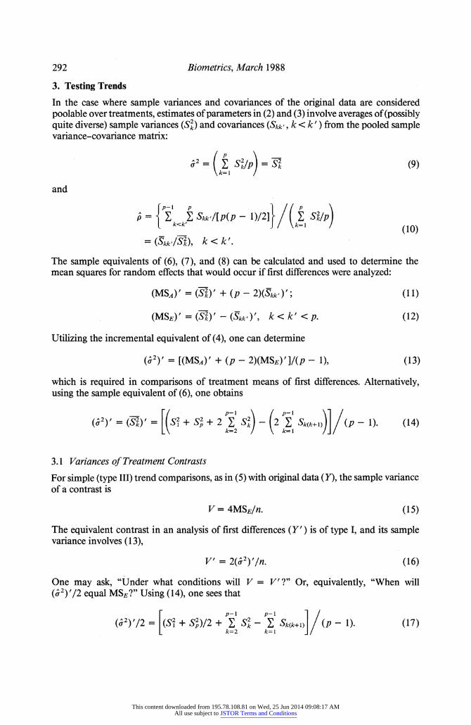
3. Testing Trends

In the case where sample variances and covariances of the original data are considered poolable over treatments, estimates of parameters in (2) and (3) involve averages of (possibly quite diverse) sample variances (Sk) and covariances (Skk', k < k') from the pooled sample variance-covariance matrix:

= (E Su/p) k (9)

and

A= <kE Skk'/[p(p - 1)/2]} ( 1E Si/p) k<k'- k=lI (10)

(kSk), k < k'.

The sample equivalents of (6), (7), and (8) can be calculated and used to determine the mean squares for random effects that would occur if first differences were analyzed:

(MSA) = (Sk) + (p - 2)(Skk); (11)

(MSE) = (Sk) - (Skk')', k < k' < p. (12)

Utilizing the incremental equivalent of (4), one can determine

a = [(MSA)' + (p - 2)(MSE)]/(P - 1), (13)

which is required in comparisons of treatment means of first differences. Alternatively, using the sample equivalent of (6), one obtains

k =[( + -2 k) (2 E Sk(k+l))1 (p - 1). (14)

3.1 Variances of Treatment Contrasts

For simple (type III) trend comparisons, as in (5) with original data (Y), the sample variance of a contrast is

V = 4MSE/n. (15)

The equivalent contrast in an analysis of first differences (Y') is of type I, and its sample variance involves (13),

V 2(2)I/n. (16)

One may ask, "Under what conditions will V = V'?" Or, equivalently, "When will (a2) '/2 equal MSE?" Using (14), one sees that

p-i p-i 1 () /2 (51+=+ S - E Sk(k+1)/ (p - 1). (17)

k=2 k=l J




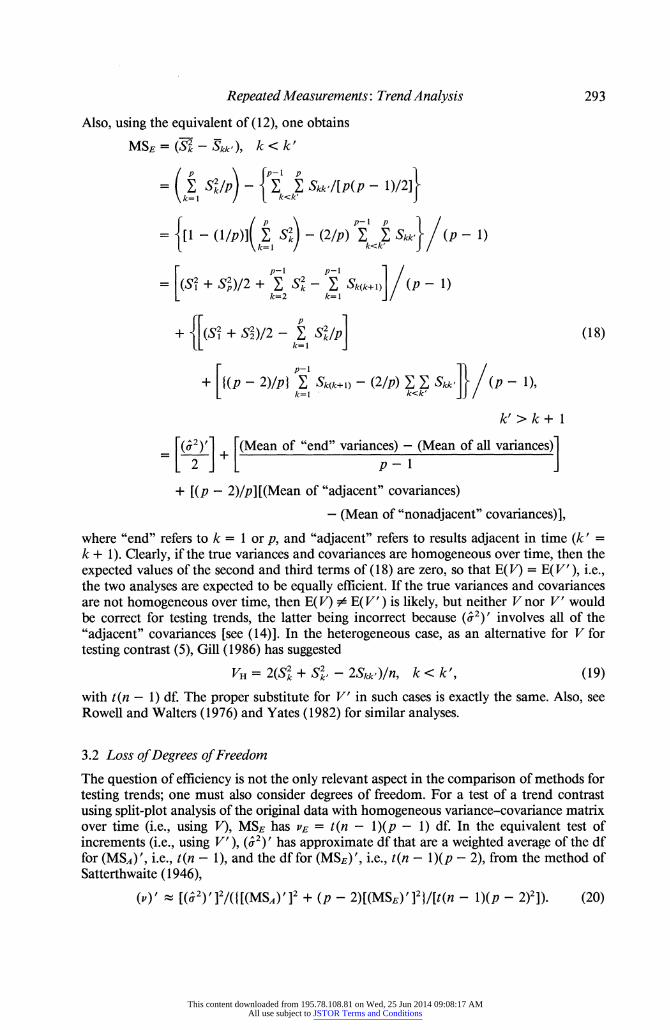
Also, using the equivalent of (12), one obtains

MSE = (S- Skk'), k < k

P 2 P-1 p

=1 k/P - k Skk[p(p - 1)/2]}

= {[1 - (1/p)I(~ ESk) - (2/p) E<kE Skk'}(p -i1)

F~2 p-l p-li = S1+Sp)/2 + E S2 -

E Sk(k+ 1) /( P-i1) k=1 k=2 k=<

r~~ ~ _- p

+ {[(s1 + S S)/2 - E s1/p] (18)

+ - 2)/p} E - (2/p) E Skk']} (P - 1),

k==I k k<k

k'S> k + 1

= [(f2)2] + [(Mean of kend" variances)- (Mean of all variances)]

+ [(p - 2)/p][(Mean of "adjacent" covariances)

- (Mean of "nonadjacent" covariances)],

where "end" refers to k = 1 or p, and "adjacent" refers to results adjacent in time (k' = k + 1). Clearly, if the true variances and covariances are homogeneous over time, then the expected values of the second and third terms of (18) are zero, so that E( V) = E( V' ), i.e., the two analyses are expected to be equally efficient. If the true variances and covariances are not homogeneous over time, then E( V) $ E( V' ) is likely, but neither V nor V' would be correct for testing trends, the latter being incorrect because (ff2)t involves all of the "adjacent" covariances [see (14)]. In the heterogeneous case, as an alternative for V for testing contrast (5), Gill (1986) has suggested

VH = 2(5k + S, - 2Skk )/n, k < k', (19)

with t(n - 1) df. The proper substitute for V' in such cases is exactly the same. Also, see Rowell and Walters (1976) and Yates (1982) for similar analyses.

3.2 Loss of Degrees of Freedom

The question of efficiency is not the only relevant aspect in the comparison of methods for testing trends; one must also consider degrees of freedom. For a test of a trend contrast using split-plot analysis of the original data with homogeneous variance-covariance matrix over time (i.e., using V), MSE has VE = t(n - l)(p - 1) df. In the equivalent test of increments (i.e., using V' ), (ff2)' has approximate df that are a weighted average of the df for (MSA)', i.e., t(n - 1), and the df for (MSE)', i.e., t(n - l)(p - 2), from the method of Satterthwaite (1946),

(V)'~ [( )'] /({[(MSA)p ] + (P - 2)[(MS2SE) ] }/[t(n - l)(p - 2)2]) (20)




Using the equivalents of (2) and (3) for incremental data, one obtains

E[(MSA)']/E[(MSE)'] = (Or2) [1 + (p - 2)p']/[(Or2)'(1 _ )] (21)

= 1 + [(p- l)p'/(l - p')].*

Suppose that p' = +.5. Then (21) becomes just p, so that E[(MSA)'] = pE[(MSE)']. Furthermore, E[(MSE)'] = (C 2) '/2 for p' = +.5. Substituting these special expectations into (20), one would expect

(v)' 4t(n - l)(p - l)2/[(p + 2)(p - 1)] = [4/(p + 2)]VE.

Thus, if the interperiod correlation for incremental data is p' = +.5, and if p > 6 periods, then the number of df for V' is likely to be less than half of VE, the number of df for V in the test of trend using the original data.

The loss of df would be especially critical in experiments with few animals (small n) and many periods. For example, if t = 2, n = 4, and p = 10, then VE = 54, but one would expect (v)' - 18 for p' = +.5. For the same example, if the interperiod correlation of increments were not so strong, say p' = +.25, then one would expect (v)' - 36; i.e., the loss of df would be less severe.

4. An Example

An experiment in mammary physiology (Paape and Tucker, 1969) involved measurement of litter weight gains for the n = 6 pregnant lactating rats (treatment group 1) and n = 6 nonpregnant lactating rats (treatment group 2). Litter size was adjusted to maintain one suckling pup per mammary gland, and litters were replaced every 4 days to maintain intense suckling stimulus. The p = 4 periods of measurement were days of lactation 8-12, 12-16, 16-20, and 20-24. Original data (Y), first differences (Y'), and sample means are shown in Table 1.

Table 1 Original data (Yijk) andfirst differences Y'k = Yijy(k+1) - Yijk) of litter weight gains (g)for pregnant

(i = 1) and nonpregnant (i = 2) lactating rats (j = 1, . .. , 6 per i) over 4-day periods (k = 1, 2, 3, 4); Paape and Tucker (1969)

Yijk Y,jk

k 1 2 3 4 1 2 3 Pregnant

j= 1 7.5 8.6 6.9 .8 +1.1 -1.7 -6.1 2 10.6 11.7 8.8 1.6 +1.1 -2.9 -7.2 3 12.4 13.0 11.0 5.6 +.6 -2.0 -5.4 4 11.5 12.6 11.1 7.5 +1.1 -1.5 -3.6 5 8.3 8.9 6.8 .5 +.6 -2.1 -6.3 6 9.2 10.1 8.6 3.8 +.9 -1.5 -4.8

Sub-means 9.92 10.82 8.87 3.30 +.90 -1.95 -5.57

Nonpregnant j= 1 13.3 13.3 12.9 11.1 +0.0 -.4 -1.8

2 10.7 10.8 10.7 9.3 +. I -.1 -1.4 3 12.5 12.7 12.0 10.1 +.2 -.7 -1.9 4 8.4 8.7 8.1 5.7 +.3 -.6 -2.4 5 9.4 9.6 8.0 3.8 +.2 -1.6 -4.2 6 11.3 11.7 10.0 8.5 +.4 -1.7 -1.5

Sub-means 10.93 11.1 3 10.28 8.08 +.20 -.85 -2.20 Means 10.42 10.98 9.58 5.69 +.55 -1.40 -3.88




Split-plot analyses of variances for Y and Y' are shown in Table 2. Results of the analysis of Y are typical for split-plot experiments with few animals: Strong evidence for period differences and for treatment-period interaction, but weak evidence for the main effect of treatments (i.e., for mean difference between pregnant and nonpregnant rats). In the analysis of Y', tests of T', P', and T'P' require different interpretation than their counterparts in the analysis of Y. The test of T' is a test of part of the interaction TP, i.e., nonparallelism of trends. The test of P' is a test of the hypothesis that mean trend over time (for both treatments combined) is linear (instead of zero, as in the test of P). The test of T'P' is a test of the hypothesis that acceleration of change is the same in the two treatment trends (instead of that the amount of change is the same, as in the test of TP).

Table 2 Split-plot analyses of variance for Y and Y' (data in Table 1)

Sources of variation Mean in Y df squares E(MS) F-ratios

Treatments (T) 1 42.56 a2(1 + 3p) + 24 j=1 T? 2.54 (n.s.) Animals/T 10 16.75 ay2(1 + 3p) Periods (P) 3 68.38 a2(1 - p) + 12 Z4 1 Pk/3 113.66 TPinteraction 3 11.83 a2(1 -p)+6E?=, Z4

(TP)2 /3 19.67 Residual error (E) 30 .60 a2(1 - p)

= [16.75 + 3(.60)]/4 = 4.64

p = (16.75 - .60)/[4(4.64)] = .87

Sources of variation Mean in Y' df squares E(MS) F-ratios

Treatments (T') 1 14.19 (o2)'(1 + 2p')+ 18 Z=1 (T')2 16.52a Animals/T' 10 .86 (ay2)'(1 + 2p') Periods (P') 2 59.25 (a 2)(1 - pI) + 12 ElI (P)2 /2 135.65 T'P' interaction 2 12.46 (a2)y(1 - p') + 6 ?=, Z4=1 (T'P')2 /2 28.52 Residual error (E') 20 .44 (a 2)'(1 _ pI)

= [.86 + 2(.44)]/3 = .58

p= (.86 - .44)/[3(.58)] = .24

a This tests interaction that is only part of the TP interaction in the analysis of Y, and with fewer df.

4.1 Correlation and Heterogeneity

As expected, analysis of first differences (Y') reduced interperiod correlation. Estimates (Table 2) are p = +.87 for original data and p = +.24 for increments. But that result does not necessarily imply that the required assumption of homogeneity of the variance- covariance matrix is better attained.

It has been shown (Gill and Hafs, 1971) that the original data have sample variance- covariance matrices that are not significantly different for pregnant and nonpregnant animals (Box test: 9.64 < X 20 = 11.78). It can be shown that a similar result applies to the first differences (Box test: 4.22 <x 30,6 = 7.23). Therefore, it is appropriate to examine variances and covariances pooled over treatments for both forms of the data. The pooled sample variance-covariance matrices (S for Y, S 'for Y') are shown in Table 3. It has been shown that S is not uniform over time (Box test: 43.58 > X01,8 = 26.12), and it can be shown that S' is not uniform either (Box test: 24.14 > xv %l 4 = 18.47). Therefore, although the use of first differences reduced interperiod sample correlation considerably, it did not eliminate the problem of heterogeneity of variances and covariances over time.




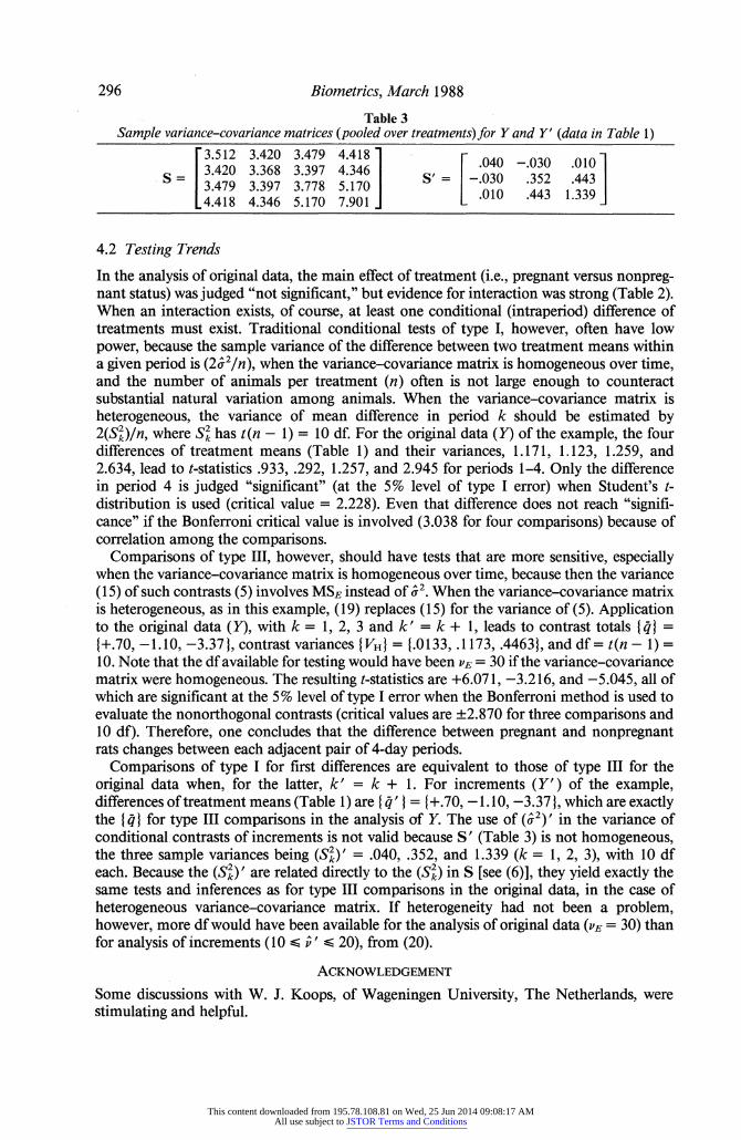
Table 3 Sample variance-covariance matrices (pooled over treatments) for Y and Y' (data in Table 1)

F3.512 3.420 3.479 4.4181[.4 -03 .11 = 3.420 3.368 3.397 4.346 = .030 .0352 .443

[4.418 4.346 51170 7.901 ] [ 010 .443 1.339 ]

4.2 Testing Trends

In the analysis of original data, the main effect of treatment (i.e., pregnant versus nonpregnant status) was judged "not significant," but evidence for interaction was strong (Table 2). When an interaction exists, of course, at least one conditional (intraperiod) difference of treatments must exist. Traditional conditional tests of type I, however, often have low power, because the sample variance of the difference between two treatment means within a given period is (20? /n), when the variance-covariance matrix is homogeneous over time, and the number of animals per treatment (n) often is not large enough to counteract substantial natural variation among animals. When the variance-covariance matrix is heterogeneous, the variance of mean difference in period k should be estimated by 2(S2)/n, where Sk has t(n - 1) = 10 df. For the original data (Y) of the example, the four differences of treatment means (Table 1) and their variances, 1.171, 1.123, 1.259, and 2.634, lead to t-statistics .933, .292, 1.257, and 2.945 for periods 1-4. Only the difference in period 4 is judged "significant" (at the 5% level of type I error) when Student's t- distribution is used (critical value = 2.228). Even that difference does not reach "signifi- cance" if the Bonferroni critical value is involved (3.038 for four comparisons) because of correlation among the comparisons.

Comparisons of type III, however, should have tests that are more sensitive, especially when the variance-covariance matrix is homogeneous over time, because then the variance (15) of such contrasts (5) involves MSE instead of a2. When the variance-covariance matrix is heterogeneous, as in this example, (19) replaces (15) for the variance of (5). Application to the original data (Y), with k = 1, 2, 3 and k' = k + 1, leads to contrast totals { fl = {+.70, -1.10, -3.371, contrast variances I VHI = {.0133, .1173, .44631, and df = t(n - 1) = 10. Note that the df available for testing would have been VE = 30 if the variance-covariance matrix were homogeneous. The resulting t-statistics are +6.071, -3.216, and -5.045, all of which are significant at the 5% level of type I error when the Bonferroni method is used to evaluate the nonorthogonal contrasts (critical values are ?2.870 for three comparisons and 10 df). Therefore, one concludes that the difference between pregnant and nonpregnant rats changes between each adjacent pair of 4-day periods.

Comparisons of type I for first differences are equivalent to those of type III for the original data when, for the latter, k' = k + 1. For increments (Y') of the example, differences of treatment means (Table 1) are 1 q' 1 = {+.70, -1.10, -3.371, which are exactly the {q} for type III comparisons in the analysis of Y. The use of (g2)' in the variance of conditional contrasts of increments is not valid because S' (Table 3) is not homogeneous, the three sample variances being (S2)' = .040, .352, and 1.339 (k = 1, 2, 3), with 10 df each. Because the (S2) ' are related directly to the (S2) in S [see (6)], they yield exactly the same tests and inferences as for type III comparisons in the original data, in the case of heterogeneous variance-covariance matrix. If heterogeneity had not been a problem, however, more df would have been available for the analysis of original data (VE = 30) than for analysis of increments (10 < v ' 20), from (20).

ACKNOWLEDGEMENT

Some discussions with W. J. Koops, of Wageningen University, The Netherlands, were stimulating and helpful.




RESUMmE

Dans les etudes portant sur des unites experimentales avec des mesures repetees, on montre que les proclamations de certains (cf. Box, 1950, Biometrics 6, 362-389), qui consistent a dire que l'analyse des accroissements de la reponse est superieure a l'analyse de la tendance sur les donnees brutes a l'aide d'un modele split-plot, sont fausses. La reduction de la correlation interperiodes (en utilisant les differences premieres) n'elimine pas necessairement les problemes lies a l'heterogeneite de la matrice de variances-covariances au cours du temps. En condition homogene, on montre' que la variance moyenne d'un simple contraste de tendance (entre deux traitements, pour des periodes consecutives) est la meme quelle que soit l'analyse, mais l'analyse des accroissements fait perdre des degres de liberte, ce qui peut etre critique dans les etudes otu l'on dispose de quelques unites experimentales par traitement. On donne un exemple de physiologie mammaire.

REFERENCES

Box, G. E. P. (1950). Problems in the analysis of growth and wear curves. Biometrics 6, 362-389. Gill, J. L. (1978). Design and Analysis of Experiments in the Animal and Medical Sciences,

Volume 2. Ames, Iowa: Iowa State University Press. Gill, J. L. (1986). Repeated measurement: Sensitive tests for experiments with few animals. Journal

ofAnimal Science 63, 943-954. Gill, J. L. and Hafs, H. D. (1971). Analysis of repeated measurements of animals. Journal ofAnimal

Science 33, 331-336. Huynh, H. and Feldt, L. S. (1970). Conditions under which mean square ratios in repeated

measurements designs have exact F-distributions. Journal of the American Statistical Association 65,1582-1589.

Koch, G. G., Amara, I. A., Stokes, M. E., and Gillings, D. (1980). Some views on parametric and nonparametric analysis for repeated measurements and selected bibliography. International Statistical Review 48, 249-265.

Paape, M. J. and Tucker, H. A. (1969). Mammary nucleic acid, hydroxyproline, and hexosamine of pregnant rats during lactation and post-lactational involution. Journal of Dairy Science 52, 380-385.

Rowell, J. G. and Walters, D. E. (1976). Analysing data with repeated observations on each experimental unit. Journal ofAgricultural Science, Cambridge 87, 423-432.

Satterthwaite, F. E. (1946). An approximate distribution of estimates of variance components. Biometrics 2, 110-114.

Yates, F. (1982). Regression models for repeated measurements. Biometrics 38, 850-853.

Received February 1986; revised September 1987.



repeated measurement: split-plot trend analysis versus analysis of first differences

Documents