remote sensing, climate and gis data analysis · remote sensing, climate and gis data analysis jay...
TRANSCRIPT

Remote Sensing, Climate and
GIS Data Analysis
Jay Angerer MOR2 Annual Meeting
June 2013
Remote Sensing • The term "remote sensing," first used in the United
States in the 1950s by Ms. Evelyn Pruitt of the U.S. Office of Naval Research
• Defined as the science—and art—of identifying, observing, and measuring an object without coming into direct contact with it.
• Involves the detection and measurement of radiation of different wavelengths reflected or emitted from distant objects or materials, by which they may be identified and categorized by class/type, substance, and spatial distribution.
From: http://earthobservatory.nasa.gov/Features/RemoteSensing/
Radiation • Unless it has a temperature of absolute zero (-
273°C) an object reflects, absorbs, and emits energy in a unique way, and at all times.
• This energy, called electromagnetic radiation, is emitted in waves that are able to transmit energy from one place to another.
• Soil, trees, air, the Sun, the Earth, and all the stars and planets are reflecting and emitting a wide range of electromagnetic waves.
From: http://earthobservatory.nasa.gov/Features/RemoteSensing/

Remote Sensing Process Example
1. Energy Source or Illumination (A)
2. Radiation and the Atmosphere (B)
3. Interaction with the Target (C)
From: http://www.nrcan.gc.ca/earth-sciences/geography-boundary/remote-sensing/fundamentals/1924/
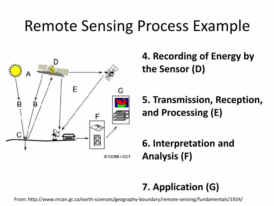
Remote Sensing Process Example
4. Recording of Energy by the Sensor (D)
5. Transmission, Reception, and Processing (E)
6. Interpretation and Analysis (F)
7. Application (G) From: http://www.nrcan.gc.ca/earth-sciences/geography-boundary/remote-sensing/fundamentals/1924/

Electromagnetic Spectrum
• Electromagnetic radiation is emitted at different wavelengths and frequencies
• Remote sensing generally involves use of the ultraviolet to microwave portions of the spectrum
From: http://www.nrcan.gc.ca/earth-sciences/geography-boundary/remote-sensing/fundamentals/1924/

Spectral Signatures
• For any given material, the amount of solar radiation that reflects, absorbs, or transmits varies with wavelength.
• This important property of matter makes it possible to identify different substances or classes and separate them by their spectral signatures (spectral curves)
From: http://www.fas.org/irp/imint/docs/rst/Intro/Part2_5.html

Spectral Signatures for Identifying Water Ponds
)2(
)3(
bRED
bNIRBandRatio
Band Ratio < 1.0 is identified as “clear water”
Cloud
Cloud Shadow

Vegetation Indices
• Uses differential between red and near infrared reflectance as measured by the satellite
• Actively growing plants show a contrast between strong absorption in the red and high reflectance in the near-infrared regions of the spectrum.
• The amount of absorption in the red and reflectance in the near-infrared varies with both the type of vegetation and the vigor of the plants.

Spectral Differences of Leaves
Source : http://rangeview.arizona.edu/Tutorials/intro.asp

NDVI Calculation
Calculated as NDVI = (NIR - VIS)/(NIR + VIS)
Source : http://earthobservatory.nasa.gov/Library/MeasuringVegetation/measuring_vegetation_2.html

!
!
!!
!
!
!
Altai
Sainshand
Mandalgobi
Arvaikheer
Dalanzadgad
Bayankhongor
NDVI – Vegetation Greenness
• Normalized Difference Vegetation Index (NDVI) is a satellite derived measurement of vegetation greenness
• NDVI is generally correlated to vegetation biomass in most regions
• Useful for many different applications

NDVI Data Sources • Advanced Very High Resolution Radiometer (AVHRR) –
Normalized Difference Vegetation Index (NDVI) data (GIMMs data) – 1981 to 2010
– 8 km resolution
– Widely used
– Available at http://www.glcf.umd.edu/data/gimms/
– New version should be available soon

Data Sources • Moderate Resolution Imaging Spectroradiometer (MODIS)
NDVI and Enhanced Vegetation Index (EVI) – 1 km, 500m, and 250 m resolution
– Available from 2000 to present
– Enhanced Vegetation Index (EVI) product builds in algorithms to adjust for soil distortions and canopy saturation
– Available from https://lpdaac.usgs.gov/get_data/data_pool
– Requires resampling and processing for use in GIS

Data Sources
• Expedited MODIS (eMODIS) – New product available from USGS
– 2000 to present
– Expedited means data are available within one day of last image acquisition in the composite window
– Resolution of 250m
– Geographic Projection
– Available for Asia region
– Download from:
– http://dds.cr.usgs.gov/emodis/CentralAsia/

Vegetation Condition Index
• Vegetation Condition Index is calculated by scaling NDVI for period of interest to the historical minimum and maximum
– (Current NDVI – minNDVI) / (maxNDVI – minNDVI) * 100
– Values less than 30 are considered drought
– Examine spatial extent and occurrence/intensity of drought for the time series

Vegetation Condition Index

Historical Time Series Analysis
• Time series analysis to examine trends in satellite greenness (NDVI) for historical record (nationwide) –Patterns of green-up and senescence
–Patterns in integrated NDVI (proxy for
biomass accumulation)
– Trends in vegetation condition index

Time Series Analysis
• TIMESAT software will be used for the developing the time series data – Calculates yearly beginning of season, end of season, amplitude,
integrated NDVI values
– Available from: http://www.nateko.lu.se/TIMESAT/timesat.asp?cat=0
Green-up End of Season
Integrated NDVI
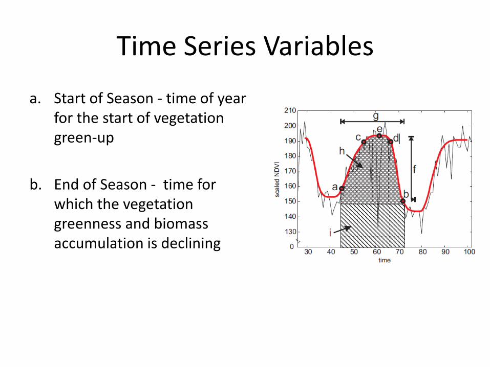
Time Series Variables
a. Start of Season - time of year for the start of vegetation green-up
b. End of Season - time for which the vegetation greenness and biomass accumulation is declining

Time Series Variables
f. Seasonal amplitude - difference between the maximum greenness value and the base level.
g. Length of the season - time from
the start to the end of the season.
h. Small Seasonal Integral - integral of the difference between the function describing the season and the base level from season start to season end.

Time Series Variables
i. Large Seasonal Integral - integral of the function describing the season from the season start to the season end.
j. Base Value - the average of the left and right minimum values – represents average of the lowest levels of NDVI for a year

Mapping Time Series Output Start of Season

Mapping Time Series Output End of Season

Mapping Time Series Output Season Large Integral

Climate Data Source and Analysis

Data Sources • Unified Precipitation Dataset
– Product available from NOAA that uses optimal interpolation
– 0.50 degree resolution (~55 km) – Daily Product, 1979 to present – Available from:
ftp://ftp.cpc.ncep.noaa.gov/precip/CPC_UNI_PRCP/GAUGE_GLB/
• Global Telecommunications System (GTS) Station Data
– Daily climate data for reporting World Meteorological Organization (WMO) stations
– Includes about 26 stations in Mongolia – Archived by Texas A&M (2003 to present) – Station History (ftp://ftp.ncdc.noaa.gov/pub/data/gsod/ish-
history.txt)

APHRODITE: Asian Precipitation - Highly-Resolved
Observational Data Integration Towards Evaluation of Water Resources
• Daily, gridded rainfall and temperature data set for Asia – Resolution: 0.25° and 0.50°
– Interpolated surfaces from a variety of climate data sources
– Time period is 1951-2007
– Monsoon Asia product
– Data Available at:
http://www.chikyu.ac.jp/precip/index.html

APHRODITE Coverage
From: http://www.chikyu.ac.jp/precip/index.html

APHRODITE Data Sources • Individual collection - Negotiation with local
meteorological/hydrological organizations and/or local researchers
• Pre-compiled datasets Global Historical Climatology Network (GHCN) Carbon Dioxide Information Analysis Center (CDIAC) National Center for Atmospheric Research, Data Archive (NCAR-DS) National Climatic Data Center (NCDC) Food and Agriculture Organization of the United Nations (FAO) GEWEX Asian Monsoon Experiment-Tropics (GAME-T) data center The Mekong River Commission (MRC) European Climate Assessment & Dataset (ECAD)
• Global Telecommunication System

World Clim Data
• Monthly interpolated surfaces of climate data
• Resolution – 1 km
• Several Variables Available:
– Min. Temperature
– Max. Temperature
– Mean Temperature
– Precipitation
– Derived Bioclimatic Variables

World Clim Data
• Monthly interpolated surfaces of climate data
• Resolution – 1 km
• Several Variables Available:
– Min. Temperature
– Max. Temperature
– Mean Temperature
– Precipitation
– Derived Bioclimatic Variables

World Clim Data
• Data Sources – – Global Historical Climatology Network (GHCN), – FAO – WMO – International Center for Tropical Agriculture (CIAT), R-Hydronet – Climate databases for Australia, New Zealand, the Nordic European
Countries, Ecuador, Peru, Bolivia, among others.
• Interpolated using the the ANUSPLIN software using latitude, longitude, and elevation as independent variables
• Time period is 1950 to 2000
• Data available online at: http://www.worldclim.org/download

Rainfall Coefficient of Variability (CV) Mapping
• The CV of annual rainfall has been suggested as a threshold indicator for equilibrium vs. non-equilibrium conditions on rangelands
• Areas having CVs of greater than 33% may be indicative of non-equilibrium conditions
• Interpolated rainfall time series provide a means to examine the spatial extent of areas having high rainfall variability
• The data can be analyze to map the CV to identify potential equilibrium/non-equilibrium zones

Rainfall CV Mapping
von Wehrden, H., J. Hanspach, P. Kaczensky, J. Fischer and K. Wesche. 2012. A global assessment of the non-equilibrium concept in rangelands. Ecological Applications, 22(2):393-399
Texas A&M splining of WMO Dataset

Unified Precipitation Data 1979 to 2012 CV
Coefficient of Variation
0 to 33%
33 to 50%
50.00000001 - 75
75.00000001 - 100
100.0000001 - 150

Comparison of 10-Year CVs
1980-1989
1985-1994 Coefficient of Variation
0 to 33%
33 to 50%
50 - 75
75 - 100
100 - 150

Comparison of 10-Year CVs
1990-1999
1995-2004
Coefficient of Variation
0 to 33%
33 to 50%
50 - 75
75 - 100
100 - 150

Comparison of 10-Year CVs 2000-2009
2003-2012
Coefficient of Variation
0 to 33%
33 to 50%
50 - 75
75 - 100
100 - 150

Next Steps
• Examine other climate data sets (WorldClim and APHRODITE) to see if similar patterns emerge.
• Compare interpolation methods

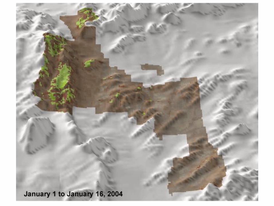
Integration with GIS and other Remote Sensing Data
• GIS provides a means of examining information in relation to boundaries, locations, and other remote sensing data
• Integration of imagery with other Remote sensing products like digital elevation models (DEM) can allow examination of data by slope, aspect, etc.

Data Data can be created in-house, downloaded, or
purchased.
Two types:
Spatial data: map, photos, graphics
Attribute data: descriptions, database
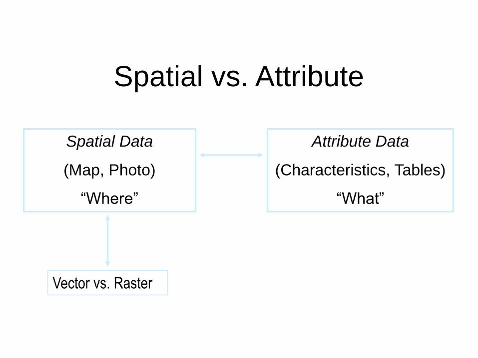
Spatial vs. Attribute
Spatial Data
(Map, Photo)
“Where”
Attribute Data
(Characteristics, Tables)
“What”
Vector vs. Raster

Spatial Data
Represented by:
Points
Lines
Polygons
Geographic representation of data
vector

Spatial Attribute
id_no name length (f)
1 Deer Trail 500
2 Spring Lane 750
3 Woods Road 1000
id_no acres infestation spread_rate
1 4 SPB 4/m
2 3.5 SPB 12/m
points
lines
polygons
points, lines, polygons
id_no nest_type eggs condition
1 rcw 4 good
2 cardinal 0 fair
3 bluebird 3 fair
4 rcw 2 good
5 cardinal 6 good
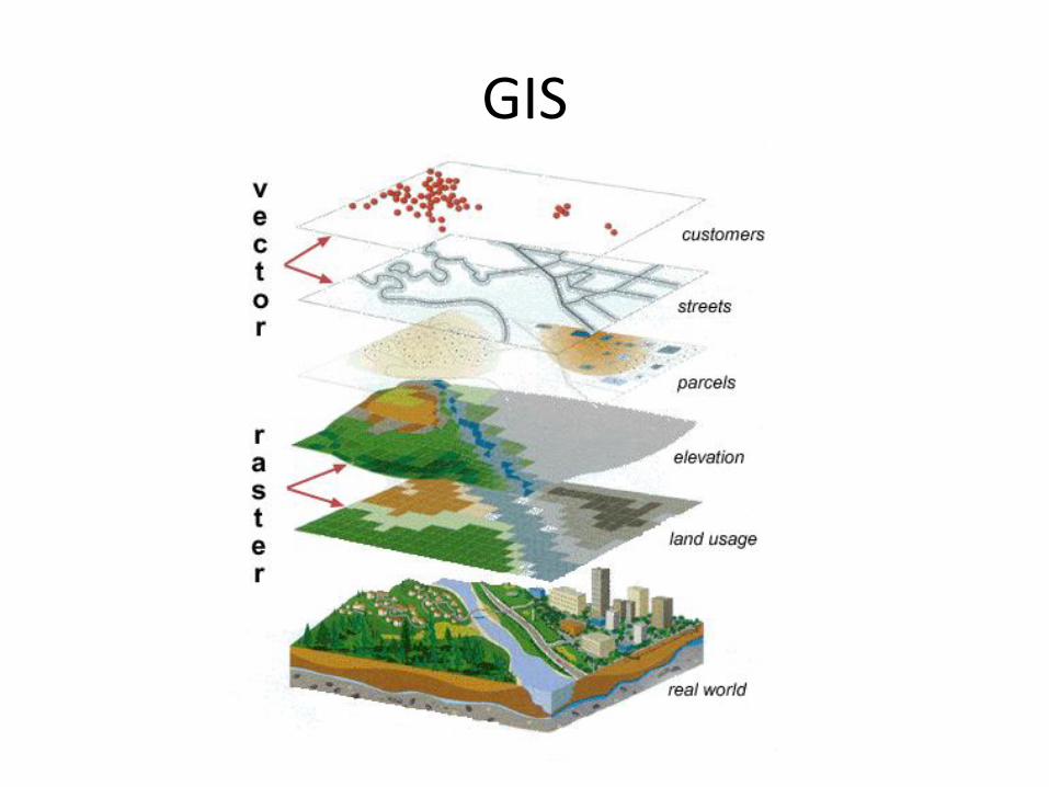
GIS

Vector Data
• Points, Lines, Polygons
• Can be used to describe real world features such as roads, property boundaries, pipelines, cities, deer blinds, transect locations, etc.
• Attributes can give details about a feature such as name, length, transect production, deer counts etc.

Example of Vector Data

Attribute Data

Raster Data
• Comprised of Pixels
• Pixel size determines resolution
• Examples:
– Satellite imagery
– Aerial Imagery
– Radar
– LIDAR

Raster Data: Resolution
35 cm 2 m 10 m 20 m

Normalized Difference Vegetation Index (NDVI) Product – 250 m resolution
Integrating Data with Boundary and Other Useful Information

Enhanced Vegetation Index (EVI) Product – 250 m resolution
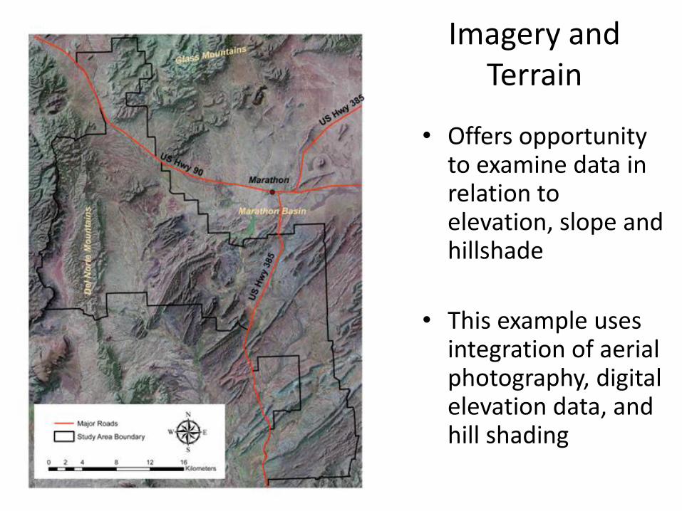
Imagery and Terrain
• Offers opportunity
to examine data in relation to elevation, slope and hillshade
• This example uses integration of aerial photography, digital elevation data, and hill shading

Integrating With a GIS

Integrating With a GIS !
!
!
!
!
!
!
!O8a
O4a
O2a
O6a
O7a
O5a
O1a

Other Products Useful For Rangelands
• Google Earth • NASA, USGS, and NOAA's Landsat satellite program
with the following sensors: – Multispectral Scanner (MSS) – Thematic Mapper (TM) and Enhanced Thematic Mapper
(ETM+) – http://landsat.usgs.gov/products_data_at_no_charge.php
• Ikonos • Quickbird • Digital Elevation Data
– Shuttle Radar Topography Mission (http://srtm.usgs.gov/index.php)
– ASTER Global Digital Elevation Map (http://asterweb.jpl.nasa.gov/gdem.asp)

Questions or Comments?