Reliable Decision Support usingCounterfactual Models

Peter SchulamDepartment of Computer Science

Johns Hopkins UniversityBaltimore, MD 21211

pschulam@cs.jhu.edu

Suchi SariaDepartment of Computer Science

Johns Hopkins UniversityBaltimore, MD 21211ssaria@cs.jhu.edu

Abstract

Decision-makers are faced with the challenge of estimating what is likely to happenwhen they take an action. For instance, if I choose not to treat this patient, are theylikely to die? Practitioners commonly use supervised learning algorithms to fitpredictive models that help decision-makers reason about likely future outcomes,but we show that this approach is unreliable, and sometimes even dangerous. Thekey issue is that supervised learning algorithms are highly sensitive to the policyused to choose actions in the training data, which causes the model to capturerelationships that do not generalize. We propose using a different learning objectivethat predicts counterfactuals instead of predicting outcomes under an existingaction policy as in supervised learning. To support decision-making in temporalsettings, we introduce the Counterfactual Gaussian Process (CGP) to predict thecounterfactual future progression of continuous-time trajectories under sequencesof future actions. We demonstrate the benefits of the CGP on two importantdecision-support tasks: risk prediction and “what if?” reasoning for individualizedtreatment planning.

1 Introduction

Decision-makers are faced with the challenge of estimating what is likely to happen when they takean action. One use of such an estimate is to evaluate risk; e.g. is this patient likely to die if I do notintervene? Another use is to perform “what if?” reasoning by comparing outcomes under alternativeactions; e.g. would changing the color or text of an ad lead to more click-throughs? Practitionerscommonly use supervised learning algorithms to help decision-makers answer such questions, butthese decision-support tools are unreliable, and can even be dangerous.

Consider, for instance, the finding discussed by Caruana et al. [2015] regarding risk of death amongthose who develop pneumonia. Their goal was to build a model that predicts risk of death for ahospitalized individual with pneumonia so that those at high-risk could be treated and those at low-riskcould be safely sent home. Their model counterintuitively learned that asthmatics are less likely todie from pneumonia. They traced the result back to an existing policy that asthmatics with pneumoniashould be directly admitted to the intensive care unit (ICU), therefore receiving more aggressivetreatment. Had this model been deployed to assess risk, then asthmatics might have received lesscare, putting them at greater risk. Caruana et al. [2015] show how these counterintuitive relationshipscan be problematic and ought to be addressed by “repairing” the model. We note, however, that theseissues stem from a deeper limitation: when training data is affected by actions, supervised learningalgorithms capture relationships caused by action policies, and these relationships do not generalizewhen the policy changes.

To build reliable models for decision support, we propose using learning objectives that predictcounterfactuals, which are collections of random variables {Y [a] : a ∈ C} used in the potential

31st Conference on Neural Information Processing Systems (NIPS 2017), Long Beach, CA, USA.

arX

iv:1

703.

1065

1v4

[st

at.M

L]

1 F

eb 2

018

●

●

●

●

●●●

●●

●

40

60

80

100

120

0 5 10 15Years Since First Symptom

PFVC

●

●

●

●

●●●

●●

●

40

60

80

100

120

0 5 10 15Years Since First Symptom

PFVC E[Y [ ] | H]

Lung

Cap

acity ●

●

●

●

●●●

●●

●

40

60

80

100

120

0 5 10 15Years Since First Symptom

PFVC

History H

Drug ADrug B

E[Y [ ] | H]

E[Y [ ] | H]

(a)

Years Since First Symptom

(b) (c)

E[Y [?] | H] E[Y [?] | H] E[Y [?] | H]

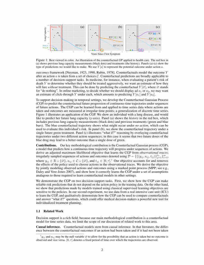
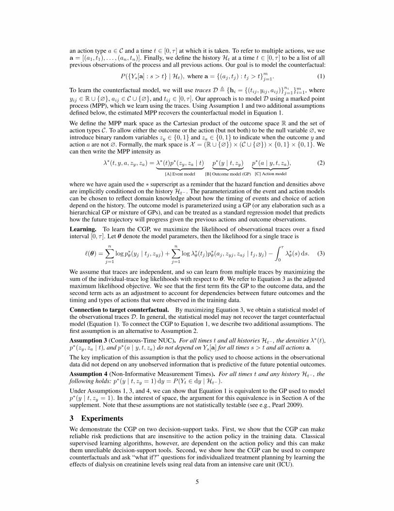
Figure 1: Best viewed in color. An illustration of the counterfactual GP applied to health care. The red box in(a) shows previous lung capacity measurements (black dots) and treatments (the history). Panels (a)-(c) show thetype of predictions we would like to make. We use Y [a] to represent the potential outcome under action a.

outcomes framework [Neyman, 1923, 1990, Rubin, 1978]. Counterfactuals model the outcome Yafter an action a is taken from a set of choices C. Counterfactual predictions are broadly applicable toa number of decision-support tasks. In medicine, for instance, when evaluating a patient’s risk ofdeath Y to determine whether they should be treated aggressively, we want an estimate of how theywill fare without treatment. This can be done by predicting the counterfactual Y [∅], where ∅ standsfor “do nothing”. In online marketing, to decide whether we should display ad a1 or a2, we may wantan estimate of click-through Y under each, which amounts to predicting Y [a1] and Y [a2].

To support decision-making in temporal settings, we develop the Counterfactual Gaussian Process(CGP) to predict the counterfactual future progression of continuous-time trajectories under sequencesof future actions. The CGP can be learned from and applied to time series data where actions aretaken and outcomes are measured at irregular time points; a generalization of discrete time series.Figure 1 illustrates an application of the CGP. We show an individual with a lung disease, and wouldlike to predict her future lung capacity (y-axis). Panel (a) shows the history in the red box, whichincludes previous lung capacity measurements (black dots) and previous treatments (green and bluebars). The blue counterfactual trajectory shows what might occur under no action, which can beused to evaluate this individual’s risk. In panel (b), we show the counterfactual trajectory under asingle future green treatment. Panel (c) illustrates “what if?” reasoning by overlaying counterfactualtrajectories under two different action sequences; in this case it seems that two future doses of theblue drug may lead to a better outcome than a single dose of green.

Contributions. Our key methodological contribution is the Counterfactual Gaussian process (CGP),a model that predicts how a continuous-time trajectory will progress under sequences of actions. Wederive an adjusted maximum likelihood objective that learns the CGP from observational traces;irregularly sampled sequences of actions and outcomes denoted using D = {{(yij , aij , tij)}ni

j=1}mi=1,where yij ∈ R ∪ {∅}, aij ∈ C ∪ {∅}, and tij ∈ [0, τ ].1 Our objective accounts for and removesthe effects of the policy used to choose actions in the observational traces. We derive the objectiveby jointly modeling observed actions and outcomes using a marked point process (MPP; see e.g.,Daley and Vere-Jones 2007), and show how it correctly learns the CGP under a set of assumptionsanalagous to those required to learn counterfactual models in other settings.

We demonstrate the CGP on two decision-support tasks. First, we show how the CGP can makereliable risk predictions that do not depend on the action policy in the training data. On the other hand,we show that predictions made by models trained using classical supervised learning objectives aresensitive to the policies. In our second experiment, we use data from a real intensive care unit (ICU)to learn the CGP, and qualitatively demonstrate how the CGP can be used to compare counterfactualsand answer “what if?” questions, which could offer medical decision-makers a powerful new tool forindividualized treatment planning.

1.1 Related Work

Decision support is a rich field; because our main methodological contribution is a counterfactualmodel for time series data, we limit the scope of our discussion of related work to this area.

Causal inference. Counterfactual models stem from causal inference. In that literature, the differ-ence between the counterfactual outcomes if an action had been taken and if it had not been taken

1yij and aij may be the null variable ∅ to allow for the possibility that an action is taken but no outcome isobserved and vice versa. [0, τ ] denotes a fixed period of time over which the trajectories are observed.

2

is defined as the causal effect of the action (see e.g., Pearl 2009 or Morgan and Winship 2014).Potential outcomes are commonly used to formalize counterfactuals and obtain causal effect estimates[Neyman, 1923, 1990, Rubin, 1978]. Potential outcomes are often applied to cross-sectional data;see, for instance, the examples in Morgan and Winship 2014. Recent examples from the machinelearning literature are Bottou et al. [2013] and Johansson et al. [2016].

Potential outcomes in discrete time. Potential outcomes have also been used to estimate the causaleffect of a sequence of actions in discrete time on a final outcome (e.g. Robins 1986, Robins andHernán 2009, Taubman et al. 2009). The key challenge in the sequential setting is to account forfeedback between intermediate outcomes that determine future treatment. Conversely, Brodersen et al.[2015] estimate the effect that a single discrete intervention has on a discrete time series. Recent workon optimal dynamic treatment regimes uses the sequential potential outcomes framework proposedby Robins [1986] to learn lists of discrete-time treatment rules that optimize a scalar outcome.Algorithms for learning these rules often use action-value functions (Q-learning; e.g., Nahum-Shaniet al. 2012). Alternatively, A-learning is a semiparametric approach that directly learns the relativedifference in value between alternative actions [Murphy, 2003].

Potential outcomes in continuous time. Others have extended the potential outcomes frameworkin Robins [1986] to learn causal effects of actions taken in continuous-time on a single final outcomeusing observational data. Lok [2008] proposes an estimator based on structural nested models[Robins, 1992] that learns the instantaneous effect of administering a single type of treatment. Arjasand Parner [2004] develop an alternative framework for causal inference using Bayesian posteriorpredictive distributions to estimate the effects of actions in continuous time on a final outcome. BothLok [2008] and Arjas and Parner [2004] use marked point processes to formalize assumptions thatmake it possible to learn causal effects from continuous-time observational data. We build on theseideas to learn causal effects of actions on continuous-time trajectories instead of a single outcome.There has also been recent work on building expressive models of treatment effects in continuoustime. Xu et al. [2016] propose a Bayesian nonparametric approach to estimating individual-specifictreatment effects of discrete but irregularly spaced actions, and Soleimani et al. [2017] model theeffects of continuous-time, continuous-valued actions. Causal effects in continuous-time have alsobeen studied using differential equations. Mooij et al. [2013] formalize an analog of Pearl’s “do”operation for deterministic ordinary differential equations. Sokol and Hansen [2014] make similarcontributions for stochastic differential equations by studying limits of discrete-time non-parametricstructural equation models [Pearl, 2009]. Cunningham et al. [2012] introduce the Causal GaussianProcess, but their use of the term “causal” is different from ours, and refers to a constraint that holdsfor sample paths of the GP.

Reinforcement learning. Reinforcement learning (RL) algorithms learn from data where actionsand observations are interleaved in discrete time (see e.g., Sutton and Barto 1998). In RL, however, thefocus is on learning a policy (a map from states to actions) that optimizes the expected reward, ratherthan a model that predicts the effects of the agent’s actions on future observations. In model-based RL,a model of an action’s effect on the subsequent state is produced as a by-product either offline beforeoptimizing the policy (e.g., Ng et al. 2006) or incrementally as the agent interacts with its environment.In most RL problems, however, learning algorithms rely on active experimentation to collect samples.This is not always possible; for example, in healthcare we cannot actively experiment on patients, andso we must rely on retrospective observational data. In RL, a related problem known as off-policyevaluation also uses retrospective observational data (see e.g., Dudík et al. 2011, Swaminathan andJoachims 2015, Jiang and Li 2016, Paduraru et al. 2012, Doroudi et al. 2017). The goal is to usestate-action-reward sequences generated by an agent operating under an unknown policy to estimatethe expected reward of a target policy. Off-policy algorithms typically use action-value functionapproximation, importance reweighting, or doubly robust combinations of the two to estimate theexpected reward.

2 Counterfactual Models from Observational TracesCounterfactual GPs build on ideas from potential outcomes [Neyman, 1923, 1990, Rubin, 1978],Gaussian processes [Rasmussen and Williams, 2006], and marked point processes [Daley and Vere-Jones, 2007]. In the interest of space, we review potential outcomes and marked point processes, butrefer the reader to Rasmussen and Williams [2006] for background on GPs.

Background: Potential Outcomes. To formalize counterfactuals, we adopt the potential outcomesframework [Neyman, 1923, 1990, Rubin, 1978], which uses a collection of random variables {Y [a] :

3

a ∈ C} to model the outcome after each action a from a set of choices C. To make counterfactualpredictions, we must learn the distribution P (Y [a] | X) for each action a ∈ C given featuresX . If wecan freely experiment by repeatedly taking actions and recording the effects, then it is straightforwardto fit a predictive model. Conducting experiments, however, may not be possible. Alternatively, wecan use observational data, where we have example actions A, outcomes Y , and features X , but donot know how actions were chosen. Note the difference between the action a and the random variableA that models the observed actions in our data; the notation Y [a] serves to distinguish between theobserved distribution P (Y | A,X) and the target distribution P (Y [a] | X).

In general, we can only use observational data to estimate P (Y | A,X). Under two assumptions,however, we can show that this conditional distribution is equivalent to the counterfactual modelP (Y [a] | X). The first is known as the Consistency Assumption.

Assumption 1 (Consistency). Let Y be the observed outcome, A ∈ C be the observed action, andY [a] be the potential outcome for action a ∈ C, then: (Y , Y [a] ) | A = a.

Under consistency, we have that P (Y | A = a) = P (Y [a] | A = a). Now, the potential outcomeY [a] may depend on the action A, so in general P (Y [a] | A = a) 6= P (Y [a]). The next assumptionposits that the features X include all possible confounders [Morgan and Winship, 2014], which aresufficient to d-separate Y [a] and A.

Assumption 2 (No Unmeasured Confounders (NUC)). Let Y be the observed outcome, A ∈ C bethe observed action, X be a vector containing all potential confounders, and Y [a] be the potentialoutcome under action a ∈ C, then: (Y [a] ⊥ A ) | X.Under Assumptions 1 and 2, P (Y | A,X) = P (Y [a] | X). An extension of Assumption 2 introducedby Robins [1997] known as sequential NUC allows us to estimate the effect of a sequence of actionsin discrete time on a single outcome. In continuous-time settings, where both the type and timingof actions may be statistically dependent on the potential outcomes, Assumption 2 (and sequentialNUC) cannot be applied as-is. We will describe an alternative that serves a similar role for CGPs.

Background: Marked Point Processes. Point processes are distributions over sequences of times-tamps {Ti}Ni=1, which we call points, and a marked point process (MPP) is a point process whereeach point is annotated with an additional random variable Xi, called its mark. For example, a pointT might represent the arrival time of a customer, and X the amount that she spent at the store. Weemphasize that both the annotated points (Ti, Xi) and the number of points N are random variables.

A point process can be characterized as a counting process {Nt : t ≥ 0} that counts the number ofpoints that occured up to and including time t: Nt =

∑Ni=1 I(Ti≤t). By definition, this processes can

only take integer values, and Nt ≥ Ns if t ≥ s. In addition, it is commonly assumed that N0 = 0 andthat ∆Nt = limδ→0+ Nt−Nt−δ ∈ {0, 1}. We can parameterize a point process using a probabilisticmodel of ∆Nt given the history of the process Ht− up to but not including time t (we use t− todenote the left limit of t). Using the Doob-Meyer decomposition [Daley and Vere-Jones, 2007], wecan write ∆Nt = ∆Mt + ∆Λt, where Mt is a martingale, Λt is a cumulative intensity function, and

P (∆Nt = 1 | Ht−) = E [∆Nt | Ht− ] = E [∆Mt | Ht− ] + ∆Λt(Ht−) = 0 + ∆Λt(Ht−),

which shows that we can parameterize the point process using the conditional intensity functionλ∗(t) dt , ∆Λt(Ht−). The star superscript on the intensity function serves as a reminder that itdepends on the historyHt− . For example, in non-homogeneous Poisson processes λ∗(t) is a functionof time that does not depend on the history. On the other hand, a Hawkes process is an example ofa point process where λ∗(t) does depend on the history [Hawkes, 1971]. MPPs are defined by anintensity that is a function of both the time t and the mark x: λ∗(t, x) = λ∗(t)p∗(x | t). We havewritten the joint intensity in a factored form, where λ∗(t) is the intensity of any point occuring (thatis, the mark is unspecified), and p∗(x | t) is the pdf of the observed mark given the point’s time. Foran MPP, the historyHt contains each prior point’s time and mark.

2.1 Counterfactual Gaussian Processes

Let {Yt : t ∈ [0, τ ]} denote a continuous-time stochastic process, where Yt ∈ R, and [0, τ ] definesthe interval over which the process is defined. We will assume that the process is observed at adiscrete set of irregular and random times {(yj , tj)}nj=1. We use C to denote the set of possible actiontypes, a ∈ C to denote the elements of the set, and define an action to be a 2-tuple (a, t) specifying

4

an action type a ∈ C and a time t ∈ [0, τ ] at which it is taken. To refer to multiple actions, we usea = [(a1, t1), . . . , (an, tn)]. Finally, we define the history Ht at a time t ∈ [0, τ ] to be a list of allprevious observations of the process and all previous actions. Our goal is to model the counterfactual:

P ({Ys[a] : s > t} | Ht), where a = {(aj , tj) : tj > t}mj=1. (1)

To learn the counterfactual model, we will use traces D , {hi = {(tij , yij , aij)}ni

j=1}mi=1, where

yij ∈ R ∪ {∅}, aij ∈ C ∪ {∅}, and tij ∈ [0, τ ]. Our approach is to model D using a marked pointprocess (MPP), which we learn using the traces. Using Assumption 1 and two additional assumptionsdefined below, the estimated MPP recovers the counterfactual model in Equation 1.

We define the MPP mark space as the Cartesian product of the outcome space R and the set ofaction types C. To allow either the outcome or the action (but not both) to be the null variable ∅, weintroduce binary random variables zy ∈ {0, 1} and za ∈ {0, 1} to indicate when the outcome y andaction a are not ∅. Formally, the mark space is X = (R ∪ {∅})× (C ∪ {∅})× {0, 1} × {0, 1}. Wecan then write the MPP intensity as

λ∗(t, y, a, zy, za) = λ∗(t)p∗(zy, za | t)︸ ︷︷ ︸[A] Event model

p∗(y | t, zy)︸ ︷︷ ︸[B] Outcome model (GP)

p∗(a | y, t, za)︸ ︷︷ ︸[C] Action model

, (2)

where we have again used the ∗ superscript as a reminder that the hazard function and densities aboveare implicitly conditioned on the historyHt− . The parameterization of the event and action modelscan be chosen to reflect domain knowledge about how the timing of events and choice of actiondepend on the history. The outcome model is parameterized using a GP (or any elaboration such as ahierarchical GP or mixture of GPs), and can be treated as a standard regression model that predictshow the future trajectory will progress given the previous actions and outcome observations.

Learning. To learn the CGP, we maximize the likelihood of observational traces over a fixedinterval [0, τ ]. Let θ denote the model parameters, then the likelihood for a single trace is

`(θ) =

n∑j=1

log p∗θ(yj | tj , zyj) +

n∑j=1

log λ∗θ(tj)p∗θ(aj , zyj , zaj | tj , yj)−

∫ τ

0

λ∗θ(s) ds. (3)

We assume that traces are independent, and so can learn from multiple traces by maximizing thesum of the individual-trace log likelihoods with respect to θ. We refer to Equation 3 as the adjustedmaximum likelihood objective. We see that the first term fits the GP to the outcome data, and thesecond term acts as an adjustment to account for dependencies between future outcomes and thetiming and types of actions that were observed in the training data.

Connection to target counterfactual. By maximizing Equation 3, we obtain a statistical model ofthe observational traces D. In general, the statistical model may not recover the target counterfactualmodel (Equation 1). To connect the CGP to Equation 1, we describe two additional assumptions. Thefirst assumption is an alternative to Assumption 2.Assumption 3 (Continuous-Time NUC). For all times t and all historiesHt− , the densities λ∗(t),p∗(zy, za | t), and p∗(a | y, t, za) do not depend on Ys[a] for all times s > t and all actions a.

The key implication of this assumption is that the policy used to choose actions in the observationaldata did not depend on any unobserved information that is predictive of the future potential outcomes.Assumption 4 (Non-Informative Measurement Times). For all times t and any history Ht− , thefollowing holds: p∗(y | t, zy = 1) dy = P (Yt ∈ dy | Ht−).

Under Assumptions 1, 3, and 4, we can show that Equation 1 is equivalent to the GP used to modelp∗(y | t, zy = 1). In the interest of space, the argument for this equivalence is in Section A of thesupplement. Note that these assumptions are not statistically testable (see e.g., Pearl 2009).

3 ExperimentsWe demonstrate the CGP on two decision-support tasks. First, we show that the CGP can makereliable risk predictions that are insensitive to the action policy in the training data. Classicalsupervised learning algorithms, however, are dependent on the action policy and this can makethem unreliable decision-support tools. Second, we show how the CGP can be used to comparecounterfactuals and ask “what if?” questions for individualized treatment planning by learning theeffects of dialysis on creatinine levels using real data from an intensive care unit (ICU).

5

Regime A Regime B Regime CBaseline GP CGP Baseline GP CGP Baseline GP CGP

Risk Score ∆ from A 0.000 0.000 0.083 0.001 0.162 0.128Kendall’s τ from A 1.000 1.000 0.857 0.998 0.640 0.562

AUC 0.853 0.872 0.832 0.872 0.806 0.829

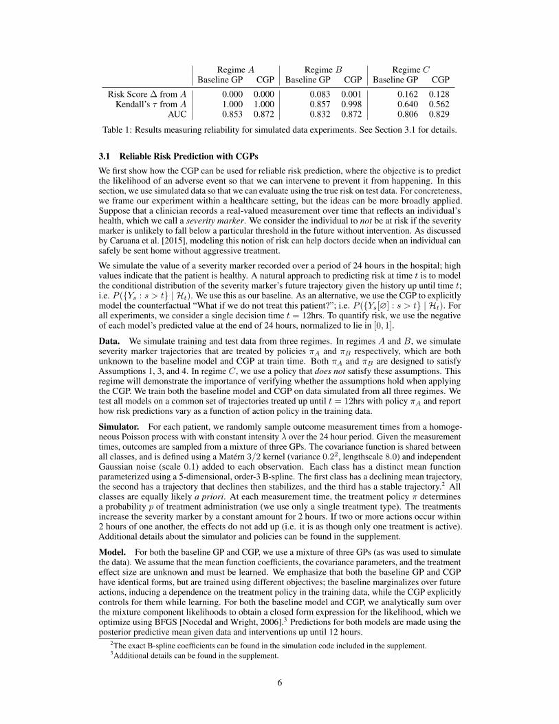
Table 1: Results measuring reliability for simulated data experiments. See Section 3.1 for details.

3.1 Reliable Risk Prediction with CGPsWe first show how the CGP can be used for reliable risk prediction, where the objective is to predictthe likelihood of an adverse event so that we can intervene to prevent it from happening. In thissection, we use simulated data so that we can evaluate using the true risk on test data. For concreteness,we frame our experiment within a healthcare setting, but the ideas can be more broadly applied.Suppose that a clinician records a real-valued measurement over time that reflects an individual’shealth, which we call a severity marker. We consider the individual to not be at risk if the severitymarker is unlikely to fall below a particular threshold in the future without intervention. As discussedby Caruana et al. [2015], modeling this notion of risk can help doctors decide when an individual cansafely be sent home without aggressive treatment.

We simulate the value of a severity marker recorded over a period of 24 hours in the hospital; highvalues indicate that the patient is healthy. A natural approach to predicting risk at time t is to modelthe conditional distribution of the severity marker’s future trajectory given the history up until time t;i.e. P ({Ys : s > t} | Ht). We use this as our baseline. As an alternative, we use the CGP to explicitlymodel the counterfactual “What if we do not treat this patient?”; i.e. P ({Ys[∅] : s > t} | Ht). Forall experiments, we consider a single decision time t = 12hrs. To quantify risk, we use the negativeof each model’s predicted value at the end of 24 hours, normalized to lie in [0, 1].

Data. We simulate training and test data from three regimes. In regimes A and B, we simulateseverity marker trajectories that are treated by policies πA and πB respectively, which are bothunknown to the baseline model and CGP at train time. Both πA and πB are designed to satisfyAssumptions 1, 3, and 4. In regime C, we use a policy that does not satisfy these assumptions. Thisregime will demonstrate the importance of verifying whether the assumptions hold when applyingthe CGP. We train both the baseline model and CGP on data simulated from all three regimes. Wetest all models on a common set of trajectories treated up until t = 12hrs with policy πA and reporthow risk predictions vary as a function of action policy in the training data.

Simulator. For each patient, we randomly sample outcome measurement times from a homoge-neous Poisson process with with constant intensity λ over the 24 hour period. Given the measurementtimes, outcomes are sampled from a mixture of three GPs. The covariance function is shared betweenall classes, and is defined using a Matérn 3/2 kernel (variance 0.22, lengthscale 8.0) and independentGaussian noise (scale 0.1) added to each observation. Each class has a distinct mean functionparameterized using a 5-dimensional, order-3 B-spline. The first class has a declining mean trajectory,the second has a trajectory that declines then stabilizes, and the third has a stable trajectory.2 Allclasses are equally likely a priori. At each measurement time, the treatment policy π determinesa probability p of treatment administration (we use only a single treatment type). The treatmentsincrease the severity marker by a constant amount for 2 hours. If two or more actions occur within2 hours of one another, the effects do not add up (i.e. it is as though only one treatment is active).Additional details about the simulator and policies can be found in the supplement.

Model. For both the baseline GP and CGP, we use a mixture of three GPs (as was used to simulatethe data). We assume that the mean function coefficients, the covariance parameters, and the treatmenteffect size are unknown and must be learned. We emphasize that both the baseline GP and CGPhave identical forms, but are trained using different objectives; the baseline marginalizes over futureactions, inducing a dependence on the treatment policy in the training data, while the CGP explicitlycontrols for them while learning. For both the baseline model and CGP, we analytically sum overthe mixture component likelihoods to obtain a closed form expression for the likelihood, which weoptimize using BFGS [Nocedal and Wright, 2006].3 Predictions for both models are made using theposterior predictive mean given data and interventions up until 12 hours.

2The exact B-spline coefficients can be found in the simulation code included in the supplement.3Additional details can be found in the supplement.

6

Hours Since ICU Admission

Cre

atin

ine

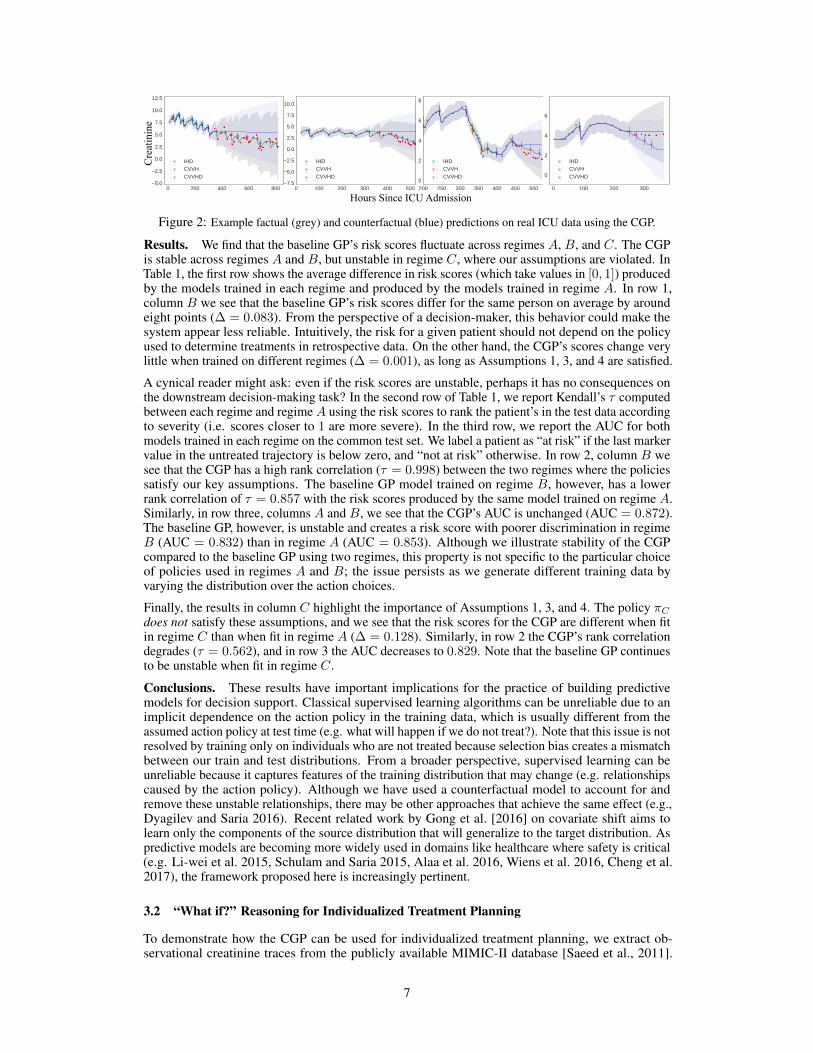
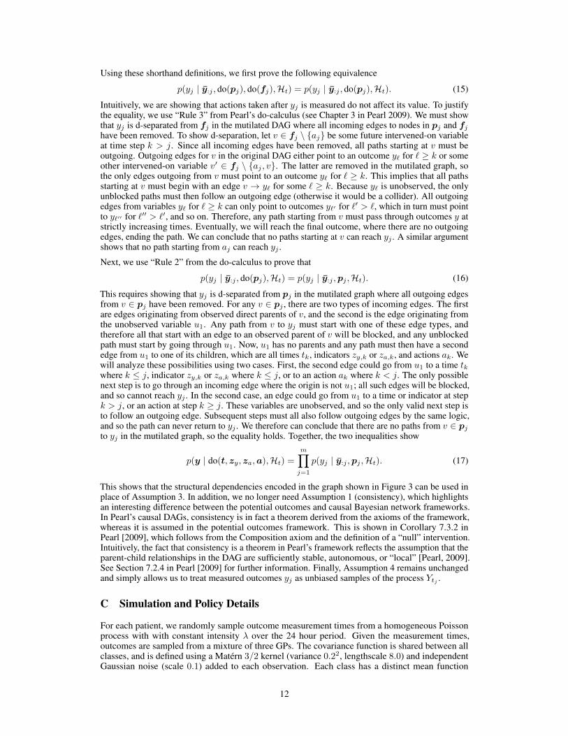
Figure 2: Example factual (grey) and counterfactual (blue) predictions on real ICU data using the CGP.

Results. We find that the baseline GP’s risk scores fluctuate across regimes A, B, and C. The CGPis stable across regimes A and B, but unstable in regime C, where our assumptions are violated. InTable 1, the first row shows the average difference in risk scores (which take values in [0, 1]) producedby the models trained in each regime and produced by the models trained in regime A. In row 1,column B we see that the baseline GP’s risk scores differ for the same person on average by aroundeight points (∆ = 0.083). From the perspective of a decision-maker, this behavior could make thesystem appear less reliable. Intuitively, the risk for a given patient should not depend on the policyused to determine treatments in retrospective data. On the other hand, the CGP’s scores change verylittle when trained on different regimes (∆ = 0.001), as long as Assumptions 1, 3, and 4 are satisfied.

A cynical reader might ask: even if the risk scores are unstable, perhaps it has no consequences onthe downstream decision-making task? In the second row of Table 1, we report Kendall’s τ computedbetween each regime and regime A using the risk scores to rank the patient’s in the test data accordingto severity (i.e. scores closer to 1 are more severe). In the third row, we report the AUC for bothmodels trained in each regime on the common test set. We label a patient as “at risk” if the last markervalue in the untreated trajectory is below zero, and “not at risk” otherwise. In row 2, column B wesee that the CGP has a high rank correlation (τ = 0.998) between the two regimes where the policiessatisfy our key assumptions. The baseline GP model trained on regime B, however, has a lowerrank correlation of τ = 0.857 with the risk scores produced by the same model trained on regime A.Similarly, in row three, columns A and B, we see that the CGP’s AUC is unchanged (AUC = 0.872).The baseline GP, however, is unstable and creates a risk score with poorer discrimination in regimeB (AUC = 0.832) than in regime A (AUC = 0.853). Although we illustrate stability of the CGPcompared to the baseline GP using two regimes, this property is not specific to the particular choiceof policies used in regimes A and B; the issue persists as we generate different training data byvarying the distribution over the action choices.

Finally, the results in column C highlight the importance of Assumptions 1, 3, and 4. The policy πCdoes not satisfy these assumptions, and we see that the risk scores for the CGP are different when fitin regime C than when fit in regime A (∆ = 0.128). Similarly, in row 2 the CGP’s rank correlationdegrades (τ = 0.562), and in row 3 the AUC decreases to 0.829. Note that the baseline GP continuesto be unstable when fit in regime C.

Conclusions. These results have important implications for the practice of building predictivemodels for decision support. Classical supervised learning algorithms can be unreliable due to animplicit dependence on the action policy in the training data, which is usually different from theassumed action policy at test time (e.g. what will happen if we do not treat?). Note that this issue is notresolved by training only on individuals who are not treated because selection bias creates a mismatchbetween our train and test distributions. From a broader perspective, supervised learning can beunreliable because it captures features of the training distribution that may change (e.g. relationshipscaused by the action policy). Although we have used a counterfactual model to account for andremove these unstable relationships, there may be other approaches that achieve the same effect (e.g.,Dyagilev and Saria 2016). Recent related work by Gong et al. [2016] on covariate shift aims tolearn only the components of the source distribution that will generalize to the target distribution. Aspredictive models are becoming more widely used in domains like healthcare where safety is critical(e.g. Li-wei et al. 2015, Schulam and Saria 2015, Alaa et al. 2016, Wiens et al. 2016, Cheng et al.2017), the framework proposed here is increasingly pertinent.

3.2 “What if?” Reasoning for Individualized Treatment Planning

To demonstrate how the CGP can be used for individualized treatment planning, we extract ob-servational creatinine traces from the publicly available MIMIC-II database [Saeed et al., 2011].

7

Creatinine is a compound produced as a by-product of the chemical reaction in the body that breaksdown creatine to fuel muscles. Healthy kidneys normally filter creatinine out of the body, which canotherwise be toxic in large concentrations. During kidney failure, however, creatinine levels rise andthe compound must be extracted using a medical procedure called dialysis.

We extract patients in the database who tested positive for abnormal creatinine levels, which is a signof kidney failure. We also extract the times at which three different types of dialysis were given toeach individual: intermittent hemodialysis (IHD), continuous veno-venous hemofiltration (CVVH),and continuous veno-venous hemodialysis (CVVHD). The data set includes a total of 428 individuals,with an average of 34 (±12) creatinine observations each. We shuffle the data and use 300 traces fortraining, 50 for validation and model selection, and 78 for testing.

Model. We parameterize the outcome model of the CGP using a mixture of GPs. We alwayscondition on the initial creatinine measurement and model the deviation from that initial value.The mean for each class is zero (i.e. we assume there is no deviation from the initial value onaverage). We parameterize the covariance function using the sum of two non-stationary kernelfunctions. Let φ : t→ [1, t, t2]> ∈ R3 denote the quadratic polynomial basis, then the first kernel isk1(t1, t2) = φ>(t1)Σφ(t2), where Σ ∈ R3×3 is a positive-definite symmetric matrix parameterizingthe kernel. The second kernel is the covariance function of the integrated Ornstein-Uhlenbeck (IOU)process (see e.g., Taylor et al. 1994), which is parameterized by two scalars α and ν and defined as

kIOU(t1, t2) = ν2

2α3

(2αmin(t1, t2) + e−αt1 + e−αt2 − 1− e−α|t1−t2|

).

The IOU covariance corresponds to the random trajectory of a particle whose velocity drifts accordingto an OU process. We assume that each creatinine measurement is observed with independentGaussian noise with scale σ. Each class in the mixture has a unique set of covariance parameters.To model the treatment effects in the outcome model, we define a short-term function and long-term response function. If an action is taken at time t0, the outcome δ = t − t0 hours later willbe additively affected by the response function g(δ;h1, a, b, h2, r) = gs(δ;h1, a, b) + g`(δ;h2, r),where h1, h2 ∈ R and a, b, r ∈ R+. The short-term and long-term response functions are definedas gs(δ;h1, a, b) = h1a

a−b(e−b·t − e−a·t

), and g`(δ : h2, r) = h2 · (1.0− e−r·t). The two response

functions are included in the mean function of the GP, and each class in the mixture has a unique setof response function parameters. We assume that Assumptions 1, 3, and 4 hold, and that the eventand action models have separate parameters, so can remain unspecified when estimating the outcomemodel. We fit the CGP outcome model using Equation 3, and select the number of classes in themixture using fit on the validation data (we choose three components).

Results. Figure 2 demonstrates how the CGP can be used to do “what if?” reasoning for treatmentplanning. Each panel in the figure shows data for an individual drawn from the test set. The greenpoints show measurements on which we condition to obtain a posterior distribution over mixture classmembership and the individual’s latent trajectory under each class. The red points are unobserved,future measurements. In grey, we show predictions under the factual sequence of actions extractedfrom the MIMIC-II database. Treatment times are shown using vertical bars marked with an “x”(color indicates which type of treatment was given). In blue, we show the CGP’s counterfactualpredictions under an alternative sequence of actions. The posterior predictive trajectory is shown forthe MAP mixture class (mean is shown by a solid grey/blue line, 95% credible intervals are shaded).

We qualitatively discuss the CGP’s counterfactual predictions, but cannot quantitatively evaluate themwithout prospective experimental data from the ICU. We can, however, measure fit on the factualdata and compare to baselines to evaluate our modeling decisions. Our CGP’s outcome model allowsfor heterogeneity in the covariance parameters and the response functions. We compare this choiceto two alternatives. The first is a mixture of three GPs that does not model treatment effects. Thesecond is a single GP that does model treatment effects. Over a 24-hour horizon, the CGP’s meanabsolute error (MAE) is 0.39 (95% CI: 0.38-0.40),4, and for predictions between 24 and 48 hoursin the future the MAE is 0.62 (95% CI: 0.60-0.64). The pairwise mean difference between the firstbaseline’s absolute errors and the CGP’s is 0.07 (0.06, 0.08) for 24 hours, and 0.09 (0.08, 0.10) for24-48 hours. The mean difference between the second baseline’s absolute errors and the CGP’s is0.04 (0.04, 0.05) for 24 hours and 0.03 (0.02, 0.04) for 24-48 hours. The improvements over thebaselines suggest that modeling treatments and heterogeneity with a mixture of GPs for the outcomemodel are useful for this problem.

495% confidence intervals computed using the pivotal bootstrap are shown in parentheses

8

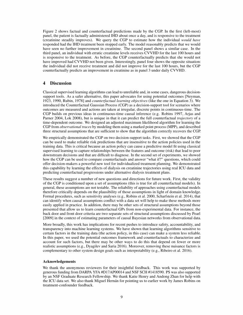
Figure 2 shows factual and counterfactual predictions made by the CGP. In the first (left-most)panel, the patient is factually administered IHD about once a day, and is responsive to the treatment(creatinine steadily improves). We query the CGP to estimate how the individual would haveresponded had the IHD treatment been stopped early. The model reasonably predicts that we wouldhave seen no further improvement in creatinine. The second panel shows a similar case. In thethird panel, an individual with erratic creatinine levels receives CVVHD for the last 100 hours andis responsive to the treatment. As before, the CGP counterfactually predicts that she would nothave improved had CVVHD not been given. Interestingly, panel four shows the opposite situation:the individual did not receive treatment and did not improve for the last 100 hours, but the CGPcounterfactually predicts an improvement in creatinine as in panel 3 under daily CVVHD.

4 Discussion

Classical supervised learning algorithms can lead to unreliable and, in some cases, dangerous decision-support tools. As a safer alternative, this paper advocates for using potential outcomes [Neyman,1923, 1990, Rubin, 1978] and counterfactual learning objectives (like the one in Equation 3). Weintroduced the Counterfactual Gaussian Process (CGP) as a decision-support tool for scenarios whereoutcomes are measured and actions are taken at irregular, discrete points in continuous-time. TheCGP builds on previous ideas in continuous-time causal inference (e.g. Robins 1997, Arjas andParner 2004, Lok 2008), but is unique in that it can predict the full counterfactual trajectory of atime-dependent outcome. We designed an adjusted maximum likelihood algorithm for learning theCGP from observational traces by modeling them using a marked point process (MPP), and describedthree structural assumptions that are sufficient to show that the algorithm correctly recovers the CGP.

We empirically demonstrated the CGP on two decision-support tasks. First, we showed that the CGPcan be used to make reliable risk predictions that are insensitive to the action policies used in thetraining data. This is critical because an action policy can cause a predictive model fit using classicalsupervised learning to capture relationships between the features and outcome (risk) that lead to poordownstream decisions and that are difficult to diagnose. In the second set of experiments, we showedhow the CGP can be used to compare counterfactuals and answer “what if?” questions, which couldoffer decision-makers a powerful new tool for individualized treatment planning. We demonstratedthis capability by learning the effects of dialysis on creatinine trajectories using real ICU data andpredicting counterfactual progressions under alternative dialysis treatment plans.

These results suggest a number of new questions and directions for future work. First, the validityof the CGP is conditioned upon a set of assumptions (this is true for all counterfactual models). Ingeneral, these assumptions are not testable. The reliability of approaches using counterfactual modelstherefore critically depends on the plausibility of those assumptions in light of domain knowledge.Formal procedures, such as sensitivity analyses (e.g., Robins et al. 2000, Scharfstein et al. 2014), thatcan identify when causal assumptions conflict with a data set will help to make these methods moreeasily applied in practice. In addition, there may be other sets of structural assumptions beyond thosepresented that allow us to learn counterfactual GPs from non-experimental data. For instance, theback door and front door criteria are two separate sets of structural assumptions discussed by Pearl[2009] in the context of estimating parameters of causal Bayesian networks from observational data.

More broadly, this work has implications for recent pushes to introduce safety, accountability, andtransparency into machine learning systems. We have shown that learning algorithms sensitive tocertain factors in the training data (the action policy, in this case) can make a system less reliable.In this paper, we used the potential outcomes framework and counterfactuals to characterize andaccount for such factors, but there may be other ways to do this that depend on fewer or morerealistic assumptions (e.g., Dyagilev and Saria 2016). Moreover, removing these nuisance factors iscomplementary to other system design goals such as interpretability (e.g., Ribeiro et al. 2016).

AcknowledgementsWe thank the anonymous reviewers for their insightful feedback. This work was supported bygenerous funding from DARPA YFA #D17AP00014 and NSF SCH #1418590. PS was also supportedby an NSF Graduate Research Fellowship. We thank Katie Henry and Andong Zhan for help withthe ICU data set. We also thank Miguel Hernán for pointing us to earlier work by James Robins ontreatment-confounder feedback.

9

A Equivalence of MPP Outcome Model and Counterfactual Model

At a given time t, we want to make predictions about the potential outcomes that we will measure ata set of future query times q = [s1, . . . , sm] given a specified future sequence of actions a. This canbe written formally as

P ({Ys[a] : s ∈ q} | Ht) (4)

Without loss of generality, we can use the chain rule to factor this joint distribution over the potentialoutcomes. We choose a factorization in time order; that is, a potential outcome is conditioned on allpotential outcomes at earlier times. We now describe a sequence of steps that we can apply to eachfactor in the product.

P ({Ys[a] : s ∈ q} | Ht) =

m∏i=1

P (Ysi [a] | {Ys[a] : s ∈ q, s < si} ,Ht). (5)

Using Assumption 3, we can introduce random variables for marked points that have the sametiming and actions as the proposed sequence of actions without changing the probability. Recall ourassumption that actions can only affect future values of the outcome, so we only need to introducemarked points for actions taken at earlier times. Formally, we introduce the set of marked points forthe potential outcome at each time si

Ai = {(t′,∅, a, 0, 1) : (t′, a) ∈ a, t′ < si} . (6)

We can then write

P (Ysi [a] | {Ys[a] : s ∈ q, s < si} ,Ht) = P (Ysi [a] | Ai, {Ys[a] : s ∈ q, s < si} ,Ht). (7)

To show that P (Y [a] | A = a,X = x) = P (Y [a] | X = x) in Section 2, we use Assumption 2 toremove the random variable A from the conditioning information without changing the probabilitystatement. We reverse that logic here by adding Ai.

Now, under Assumption 1, after conditioning on Ai, we can replace the potential outcome Ysi [a]with Ysi . We therefore have

P (Ysi [a] | Ai, {Ys[a] : s ∈ q, s < si} ,Ht) = P (Ysi | Ai, {Ys[a] : s ∈ q, s < si} ,Ht). (8)

Similarly, because the set of proposed actions affecting the outcome at time si contain all actionsthat affect the outcome at earlier times s < si, we can invoke Assumption 1 again and replace allpotential outcomes at earlier times with the value of the observed process at that time.

P (Ysi | Ai, {Ys[a] : s ∈ q, s < si} ,Ht) = P (Ysi | Ai, {Ys : s ∈ q, s < si} ,Ht).

Next, Assumption 4 posits that the outcome model p∗(y | t′, zy = 1) is the density of P (Yt′ | Ht),which implies that the mark (t′, y,∅, 1, 0) is equivalent to the event (Yt′ ∈ dy). Therefore, for eachsi define

Oi = {(s, Ys,∅, 1, 0) : s ∈ q, s < si} . (9)

Using this definition, we can write

P (Ysi | Ai, {Ys : s ∈ q, s < si} ,Ht) = (Ysi | Ai,Oi,Ht).

The set of information (Ai,Oi,Ht) is a valid history of the marked point processH−si up to but notincluding time si. We can therefore replace all information after the conditioning bar in each factorof Equation 5 withHs−i .

P (Ysi | Ai,Oi,Ht) = P (Ysi | H−si). (10)

Finally, by applying Assumption 4 again, we have

P (Ysi ∈ dy | H−si) = p∗(y | si, zy = 1) dy. (11)

The potential outcome query can therefore be answered using the outcome model, which we canestimate from data.

10

jk < j

{t, zy, za} {t, zy, za}

y y

a a

u1 u2

Figure 3: The causal Bayesian network for the counterfactual GP.

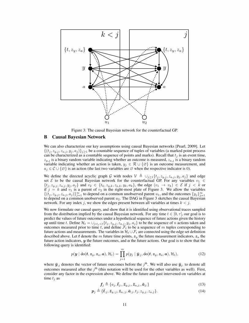
B Causal Bayesian Network

We can also characterize our key assumptions using causal Bayesian networks [Pearl, 2009]. Let{(tj , zy,j , za,j , yj , aj)}j≥1 be a countable sequence of tuples of variables (a marked point processcan be characterized as a countable sequence of points and marks). Recall that tj is an event time,zy,j is a binary random variable indicating whether an outcome is measured, za,j is a binary randomvariable indicating whether an action is taken, yj ∈ R ∪ {∅} is an outcome measurement, andaj ∈ C ∪ {∅} is an action (the last two variables are ∅ when the respective indicator is 0).

We define the directed acyclic graph G with nodes V , ∪j≥1{tj , zy,j , za,j , yj , aj} and edgeset E to be the causal Bayesian network for the counterfactual GP. For any variables v1 ∈{tj , zy,j , za,j , yj , aj} and v2 ∈ {tk, zy,k, za,k, yk, ak}, the edge (v1 → vk) ∈ E if j < k orif j = k and v1 is a parent of v2 in the right-most plate of Figure 3. We allow the variables{(tj , zy,j , za,j , aj)}∞j=1 to depend on a common unobserved parent u1, and the outcomes {yj}∞j=1to depend on a common unobserved parent u2. The DAG in Figure 3 sketches the causal Bayesiannetwork. For any index j, we show the edges present between all variables at times k < j.

We now formulate our causal query, and show that it is identified using observational traces sampledfrom the distribution implied by the causal Bayesian network. For any time t ∈ [0, τ ], our goal is topredict the values of future outcomes under a hypothetical sequence of future actions given the historyup until time t. DefineHt = ∪j:tj<t{tj , zy,j , za,j , yj , aj} to be the sequence of n actions taken andoutcomes measured prior to time t, and define Ft to be a sequence of m tuples corresponding tofuture actions and measurements. The variables inHt∪Ft are connected using the edge set definitiondescribed above. Let t denote the m future time points, zy the future measurement indicators, za thefuture action indicators, y the future outcomes, and a the future actions. Our goal is to show that thefollowing query is identified:

p(y | do(t, zy, za,a),Ht) =

m∏j=1

p(yj | y:j , do(t, zy, za,a),Ht), (12)

where y:j denotes the vector of future outcomes before the jth. We will also use yj: to denote alloutcomes measured after the jth (this notation will be used for the other variables as well). First,consider any factor in the expression above. We define the future and past intervened-on variables attime tj as

fj , {aj , tj:, zy,j:, za,j:, aj:} (13)

pj , {t:j , zy,:j , za,:j , a:j , tj , zy,j , za,j}. (14)

11

Using these shorthand definitions, we first prove the following equivalence

p(yj | y:j , do(pj), do(fj),Ht) = p(yj | y:j , do(pj),Ht). (15)

Intuitively, we are showing that actions taken after yj is measured do not affect its value. To justifythe equality, we use “Rule 3” from Pearl’s do-calculus (see Chapter 3 in Pearl 2009). We must showthat yj is d-separated from fj in the mutilated DAG where all incoming edges to nodes in pj and fjhave been removed. To show d-separation, let v ∈ fj \ {aj} be some future intervened-on variableat time step k > j. Since all incoming edges have been removed, all paths starting at v must beoutgoing. Outgoing edges for v in the original DAG either point to an outcome y` for ` ≥ k or someother intervened-on variable v′ ∈ fj \ {aj , v}. The latter are removed in the mutilated graph, sothe only edges outgoing from v must point to an outcome y` for ` ≥ k. This implies that all pathsstarting at v must begin with an edge v → y` for some ` ≥ k. Because y` is unobserved, the onlyunblocked paths must then follow an outgoing edge (otherwise it would be a collider). All outgoingedges from variables y` for ` ≥ k can only point to outcomes y`′ for `′ > `, which in turn must pointto y`′′ for `′′ > `′, and so on. Therefore, any path starting from v must pass through outcomes y atstrictly increasing times. Eventually, we will reach the final outcome, where there are no outgoingedges, ending the path. We can conclude that no paths starting at v can reach yj . A similar argumentshows that no path starting from aj can reach yj .

Next, we use “Rule 2” from the do-calculus to prove that

p(yj | y:j , do(pj),Ht) = p(yj | y:j ,pj ,Ht). (16)

This requires showing that yj is d-separated from pj in the mutilated graph where all outgoing edgesfrom v ∈ pj have been removed. For any v ∈ pj , there are two types of incoming edges. The firstare edges originating from observed direct parents of v, and the second is the edge originating fromthe unobserved variable u1. Any path from v to yj must start with one of these edge types, andtherefore all that start with an edge to an observed parent of v will be blocked, and any unblockedpath must start by going through u1. Now, u1 has no parents and any path must then have a secondedge from u1 to one of its children, which are all times tk, indicators zy,k or za,k, and actions ak. Wewill analyze these possibilities using two cases. First, the second edge could go from u1 to a time tkwhere k ≤ j, indicator zy,k or za,k where k ≤ j, or to an action ak where k < j. The only possiblenext step is to go through an incoming edge where the origin is not u1; all such edges will be blocked,and so cannot reach yj . In the second case, an edge could go from u1 to a time or indicator at stepk > j, or an action at step k ≥ j. These variables are unobserved, and so the only valid next step isto follow an outgoing edge. Subsequent steps must all also follow outgoing edges by the same logic,and so the path can never return to yj . We therefore can conclude that there are no paths from v ∈ pjto yj in the mutilated graph, so the equality holds. Together, the two inequalities show

p(y | do(t, zy, za,a),Ht) =

m∏j=1

p(yj | y:j ,pj ,Ht). (17)

This shows that the structural dependencies encoded in the graph shown in Figure 3 can be used inplace of Assumption 3. In addition, we no longer need Assumption 1 (consistency), which highlightsan interesting difference between the potential outcomes and causal Bayesian network frameworks.In Pearl’s causal DAGs, consistency is in fact a theorem derived from the axioms of the framework,whereas it is assumed in the potential outcomes framework. This is shown in Corollary 7.3.2 inPearl [2009], which follows from the Composition axiom and the definition of a “null” intervention.Intuitively, the fact that consistency is a theorem in Pearl’s framework reflects the assumption that theparent-child relationships in the DAG are sufficiently stable, autonomous, or “local” [Pearl, 2009].See Section 7.2.4 in Pearl [2009] for further information. Finally, Assumption 4 remains unchangedand simply allows us to treat measured outcomes yj as unbiased samples of the process Ytj .

C Simulation and Policy Details

For each patient, we randomly sample outcome measurement times from a homogeneous Poissonprocess with with constant intensity λ over the 24 hour period. Given the measurement times,outcomes are sampled from a mixture of three GPs. The covariance function is shared between allclasses, and is defined using a Matérn 3/2 kernel (variance 0.22, lengthscale 8.0) and independentGaussian noise (scale 0.1) added to each observation. Each class has a distinct mean function

12

parameterized using a 5-dimensional, order-3 B-spline. The first class has a declining mean trajectory,the second has a trajectory that declines then stabilizes, and the third has a stable trajectory.5 Allclasses are equally likely a priori. At each measurement time, the treatment policy π determinesa probability p of treatment administration (we use only a single treatment type). The treatmentsincrease the severity marker by a constant amount for 2 hours. If two or more actions occur within2 hours of one another, the effects do not add up (i.e. it is as though only one treatment is active).Additional details about the simulator and policies can be found in the supplement.

Policies πA and πB determine a probability of treatment at each outcome measurement time. Theyeach use the average of the observed outcomes over the previous two hours, which we denote usingy(t−2):t, as a feature, which is then multiplied by a weight wA = −0.5 (wB = 0.5 for regime B) andpassed through the inverse logit to determine a probabilty. The policy πC for regime C depends onthe patient’s latent class. The probability of treatment at any time t is p = αzσ(wA · y(t−2):t), whereαz ∈ (0, 1) is a weight that depends on the latent class z. We set α1 = 0.2, α2 = 0.9, and α3 = 0.5.

D Mixture Estimation Details

For both the simulated and real data experiments, we analytically sum over the component-specificdensities to obtain an explicit mixture density involving no latent variables. We then estimate theparameters using maximum likelihood. The likelihood surface is highly non-convex. To account forthis, we used different parameter initialization strategies for the simulated and real data.

On the simulated data experiments, the mixture components for both the CGP and baseline GPare primarily distinguished by the mean functions. We initialize the mean parameters for both thebaseline GP and CGP by first fitting a linear mixed model with B-spline bases using the EM algorithm,computing MAP estimates of trace-specific coefficients, clustering the coefficients, and initializingwith the cluster centers.

On the real data, traces have similar mean behavior (trajectories drift around the initial creatininevalue), but differed by length and amplitude of variations from the mean. We therefore centeredeach trace around its initial creatinine measurement (which we condition on), and use a meanfunction that includes only the short-term and long-term response functions. For each mixture, theresponse function parameters are initialized randomly: parameters a, b, and r are initialized usinga LogNormal(mean = 0.0, std = 0.1); heights h1 and h2 are initialized using a Normal(mean =0.0, std = 0.1). For each mixture, Σ (L300) is initialized to the identity matrix; α and ν are drawnfrom a LogNormal(mean = 0.0, std = 0.1).

ReferencesA.M. Alaa, J. Yoon, S. Hu, and M. van der Schaar. Personalized Risk Scoring for Critical Care

Patients using Mixtures of Gaussian Process Experts. In ICML Workshop on ComputationalFrameworks for Personalization, 2016.

E. Arjas and J. Parner. Causal reasoning from longitudinal data. Scandinavian Journal of Statistics,31(2):171–187, 2004.

L. Bottou, J. Peters, J.Q. Candela, D.X. Charles, M. Chickering, E. Portugaly, D. Ray, P.Y. Simard,and E. Snelson. Counterfactual reasoning and learning systems: the example of computationaladvertising. Journal of Machine Learning Research (JMLR), 14(1):3207–3260, 2013.

K.H. Brodersen, F. Gallusser, J. Koehler, N. Remy, and S.L. Scott. Inferring causal impact usingbayesian structural time-series models. The Annals of Applied Statistics, 9(1):247–274, 2015.

R. Caruana, Y. Lou, J. Gehrke, P. Koch, M. Sturm, and N. Elhadad. Intelligible models for healthcare:Predicting pneumonia risk and hospital 30-day readmission. In International Conference onKnowledge Discovery and Data Mining (KDD), pages 1721–1730. ACM, 2015.

L.F. Cheng, G. Darnell, C. Chivers, M.E. Draugelis, K. Li, and B.E. Engelhardt. Sparse multi-outputGaussian processes for medical time series prediction. arXiv preprint arXiv:1703.09112, 2017.

5The exact B-spline coefficients can be found in the simulation code included in the supplement.

13

J. Cunningham, Z. Ghahramani, and C.E. Rasmussen. Gaussian processes for time-marked time-series data. In International Conference on Artificial Intelligence and Statistics (AISTATS), pages255–263, 2012.

D.J. Daley and D. Vere-Jones. An Introduction to the Theory of Point Processes. Springer Science &Business Media, 2007.

S. Doroudi, P.S. Thomas, and E. Brunskill. Importance sampling for fair policy selection. InUncertainty in Artificial Intelligence (UAI), 2017.

M. Dudík, J. Langford, and L. Li. Doubly robust policy evaluation and learning. In InternationalConference on Machine Learning (ICML), 2011.

K. Dyagilev and S. Saria. Learning (predictive) risk scores in the presence of censoring due tointerventions. Machine Learning, 102(3):323–348, 2016.

M. Gong, K. Zhang, T. Liu, D. Tao, C. Glymour, and B. Schölkopf. Domain adaptation withconditional transferable components. In International Conference on Machine Learning (ICML),2016.

A.G. Hawkes. Spectra of some self-exciting and mutually exciting point processes. Biometrika,pages 83–90, 1971.

N. Jiang and L. Li. Doubly robust off-policy value evaluation for reinforcement learning. InInternational Conference on Machine Learning (ICML), pages 652–661, 2016.

F.D. Johansson, U. Shalit, and D. Sontag. Learning representations for counterfactual inference. InInternational Conference on Machine Learning (ICML), 2016.

H.L Li-wei, R.P. Adams, L. Mayaud, G.B. Moody, A. Malhotra, R.G. Mark, and S. Nemati. Aphysiological time series dynamics-based approach to patient monitoring and outcome prediction.IEEE Journal of Biomedical and Health Informatics, 19(3):1068–1076, 2015.

J.J. Lok. Statistical modeling of causal effects in continuous time. The Annals of Statistics, pages1464–1507, 2008.

J.M. Mooij, D. Janzing, and B. Schölkopf. From ordinary differential equations to structural causalmodels: the deterministic case. 2013.

S.L. Morgan and C. Winship. Counterfactuals and causal inference. Cambridge University Press,2014.

S.A. Murphy. Optimal dynamic treatment regimes. Journal of the Royal Statistical Society: Series B(Statistical Methodology), 65(2):331–355, 2003.

I. Nahum-Shani, M. Qian, D. Almirall, W.E. Pelham, B. Gnagy, G.A. Fabiano, J.G. Waxmonsky,J. Yu, and S.A. Murphy. Q-learning: A data analysis method for constructing adaptive interventions.Psychological Methods, 17(4):478, 2012.

J. Neyman. Sur les applications de la théorie des probabilités aux experiences agricoles: Essai desprincipes. Roczniki Nauk Rolniczych, 10:1–51, 1923.

J. Neyman. On the application of probability theory to agricultural experiments. Statistical Science,5(4):465–472, 1990.

A.Y. Ng, A. Coates, M. Diel, V. Ganapathi, J. Schulte, B. Tse, E. Berger, and E. Liang. Autonomousinverted helicopter flight via reinforcement learning. In Experimental Robotics IX, pages 363–372.Springer, 2006.

J. Nocedal and S.J. Wright. Numerical optimization 2nd, 2006.

C. Paduraru, D. Precup, J. Pineau, and G. Comanici. An empirical analysis of off-policy learning indiscrete mdps. In Workshop on Reinforcement Learning, page 89, 2012.

J. Pearl. Causality: models, reasoning and inference. Cambridge University Press, 2009.

14

C.E. Rasmussen and C.K.I. Williams. Gaussian processes for machine learning. the MIT Press,2006.

M.T. Ribeiro, S. Singh, and C. Guestrin. Why should i trust you?: Explaining the predictions of anyclassifier. In International Conference on Knowledge Discovery and Data Mining (KDD), pages1135–1144. ACM, 2016.

J.M. Robins. A new approach to causal inference in mortality studies with a sustained exposureperiod—application to control of the healthy worker survivor effect. Mathematical Modelling, 7(9-12):1393–1512, 1986.

J.M. Robins. Estimation of the time-dependent accelerated failure time model in the presence ofconfounding factors. Biometrika, 79(2):321–334, 1992.

J.M. Robins. Causal inference from complex longitudinal data. In Latent variable modeling andapplications to causality, pages 69–117. Springer, 1997.

J.M. Robins and M.A. Hernán. Estimation of the causal effects of time-varying exposures. Longitudi-nal data analysis, pages 553–599, 2009.

J.M. Robins, A. Rotnitzky, and D.O. Scharfstein. Sensitivity analysis for selection bias and un-measured confounding in missing data and causal inference models. In Statistical models inepidemiology, the environment, and clinical trials, pages 1–94. Springer, 2000.

D.B. Rubin. Bayesian inference for causal effects: The role of randomization. The Annals of statistics,pages 34–58, 1978.

M. Saeed, M. Villarroel, A.T. Reisner, G. Clifford, L.W. Lehman, G. Moody, T. Heldt, T.H. Kyaw,B. Moody, and R.G. Mark. Multiparameter intelligent monitoring in intensive care II (MIMIC-II):a public-access intensive care unit database. Critical Care Medicine, 39(5):952, 2011.

D. Scharfstein, A. McDermott, W. Olson, and F. Wiegand. Global sensitivity analysis for repeatedmeasures studies with informative dropout: A fully parametric approach. Statistics in Biopharma-ceutical Research, 6(4):338–348, 2014.

P. Schulam and S. Saria. A framework for individualizing predictions of disease trajectories byexploiting multi-resolution structure. In Advances in Neural Information Processing Systems(NIPS), pages 748–756, 2015.

A. Sokol and N.R. Hansen. Causal interpretation of stochastic differential equations. ElectronicJournal of Probability, 19(100):1–24, 2014.

H. Soleimani, A. Subbaswamy, and S. Saria. Treatment-response models for counterfactual reasoningwith continuous-time, continuous-valued interventions. In Uncertainty in Artificial Intelligence(UAI), 2017.

R.S. Sutton and A.G. Barto. Reinforcement learning: An introduction, volume 1. MIT pressCambridge, 1998.

A. Swaminathan and T. Joachims. Counterfactual risk minimization. In International Conference onMachine Learning (ICML), 2015.

S.L. Taubman, J.M. Robins, M.A. Mittleman, and M.A. Hernán. Intervening on risk factors forcoronary heart disease: an application of the parametric g-formula. International Journal ofEpidemiology, 38(6):1599–1611, 2009.

J. Taylor, W. Cumberland, and J. Sy. A stochastic model for analysis of longitudinal AIDS data.Journal of the American Statistical Association, 89(427):727–736, 1994.

J. Wiens, J. Guttag, and E. Horvitz. Patient risk stratification with time-varying parameters: amultitask learning approach. Journal of Machine Learning Research (JMLR), 17(209):1–23, 2016.

Y. Xu, Y. Xu, and S. Saria. A Bayesian nonparametric approach for estimating individualizedtreatment-response curves. In Machine Learning for Healthcare Conference (MLHC), pages282–300, 2016.

15