Relationships between the anisotropy parameters for transverselyisotropic mudrocks

Fuyong Yan1, Lev Vernik2, and De-Hua Han1

ABSTRACT

Studying the empirical relations between seismic anisotropyparameters is important for the simplification and practical ap-plications of seismic anisotropy. The elastic properties of mu-drocks are often described by transverse isotropy. Knowingthe elastic properties in the vertical and horizontal directions,a sole oblique anisotropy parameter determines the pattern ofvariation of the elastic properties of a transversely isotropic (TI)medium in all of the other directions. The oblique seismicanisotropy parameter δ, which determines seismic reflectionmoveout behavior, is important in anisotropic seismic dataprocessing and interpretation. Compared to the other anisotropyparameters, the oblique anisotropy parameter is more sensitive

to the measurement error. Although, theoretically, only oneoblique velocity is needed to determine the oblique anisotropyparameter, the uncertainty can be greatly reduced if multipleoblique velocities in different directions are measured. If a mu-drock is not a perfect TI medium but it is expediently treated asone, then multiple oblique velocity measurements in differentdirections should lead to a more representative approximationof δ or c13 because the directional bias can be reduced. Basedon a data quality analysis of the laboratory seismic anisotropymeasurement data from the literature, we found that there arestrong correlations between the oblique anisotropy parameterand the principal anisotropy parameters when data points ofmore uncertainty are excluded. Examples of potential applica-tions of these empirical relations are discussed.

INTRODUCTION

Shales or mudstones account for most of the bulk volume of sedi-mentary rocks and are the primary factor of seismic anisotropy inseismic exploration (Schoenberg et al., 1996). Shales are tradition-ally treated as the organic source rocks and seals of the petroleumreservoir. They are becoming important petroleum reservoir rockswith the advancing techniques in directional drilling and hydraulicfracturing. Understanding the elastic properties of shales is of greatconsequence in petroleum exploration. The elastic properties ofshales are often described by transverse isotropy (Johnston andChristensen, 1995; Vernik and Liu, 1997; Jakobsen and Johansen,2000; Wang, 2002; Sone, 2012). The elastic properties of a trans-versely isotropic (TI) medium are defined by five independentparameters. Relative to isotropic media whose elastic properties aredetermined by two independent parameters, including extra aniso-tropy parameter brings up great challenges in seismic data process-

ing and interpretation. For isotropic rocks, although the elastic prop-erties are defined by only two theoretically independent parameters(VP and VS), there are often strong correlations between them forthe same type of sedimentary rocks (Castagna et al., 1985). Thesecorrelations are critical for the successful application of amplitudevariation with offset interpretation techniques. With more unknownparameters in anisotropic seismic data processing and interpreta-tion, finding the relationships between the anisotropy parameterscould be vital for practical applications of seismic anisotropy.It is well-known that the P-wave velocity or modulus has a strong

correlation with the S-wave velocity or modulus in either the ver-tical or horizontal directions for mudstones (Castagna et al., 1985;Horne, 2013). Using velocity anisotropy data of various sources(primarily laboratory core data, and other data from cross-dipolesonic, crosswell, and walkaway vertical seismic profile), Horne(2013) statistically studies the relationships among the anisotropicparameters. It is found that c11 and c66 and c33 and c44 have good

Manuscript received by the Editor 8 February 2019; revised manuscript received 19 July 2019; published ahead of production 29 August 2019.1University of Houston, Department of Earth and Atmospheric Sciences, Houston, Texas, USA. E-mail: yanfyon@yahoo.com (corresponding author);

dhan@uh.edu.2Ikon Science, Houston, Texas, USA. E-mail: verniklev@gmail.com.© 2019 Society of Exploration Geophysicists. All rights reserved.

1

GEOPHYSICS, VOL. 84, NO. 6 (NOVEMBER-DECEMBER 2019); P. 1–9, 14 FIGS.10.1190/GEO2019-0088.1

correlations. The relationships between c13 and the other elasticconstants are not clear.The oblique stiffness c13 determines the pattern of variation of the

elastic properties from the vertical direction to the horizontal direc-tion for a TI medium. Laboratory estimation of c13 requires at leastone oblique velocity measurement. This oblique velocity can be aquasi-P-wave or a quasi-S-wave. A quasi-P-wave is commonly usedbecause it is usually the first-arrived signal and is favorable for ac-curate traveltime picking. The propagating direction of a quasi-P-wave is different with the direction of the particle motion. They arerelated to two velocity vectors, phase velocity and group velocity.They are different in direction and magnitude. Failure to understandthe differences and the special requirements on the measurementsetup may introduce significant uncertainty in estimating c13 andδ (Yan et al., 2016, 2018). In this study, we primarily study the re-lationship between the elastic moduli and combinations thereofmeasured in the oblique and principal directions with respect of thesymmetry elements of a TI medium based on the analysis of thelaboratory anisotropy measurement data from the literature.

THEORY

The elastic properties of a TI medium are specified by five in-dependent elastic constants. Using the Voigt notation, the elasticstiffness tensor of a TI medium with a symmetry axis aligned inthe x3-direction is expressed by

C ¼

0BBBBBB@

c11 c11 − 2c66 c13 0 0 0

c11 − 2c66 c11 c13 0 0 0

c13 c13 c33 0 0 0

0 0 0 c44 0 0

0 0 0 0 c44 0

0 0 0 0 0 c66

1CCCCCCA:

(1)

The concept of Poisson’s ratio for an isotropic medium can bestraightforwardly extended to a TI medium using Hooke’s law (King,1964; Yan et al., 2016). Their relations with the TI elastic constantsare as follows:

EV ¼ c33ðc11−c66Þ − c213c11−c66

ð¼ E3Þ; (2)

EH ¼ 4c66ðc33ðc11−c66Þ − c213Þc11c33−c213

ð¼ E1¼ E2Þ; (3)

νV ¼ c132ðc11 − c66Þ

ð¼ ν31 ¼ ν32Þ; (4)

νHV ¼ 2c13c66

c11c33−c213ð¼ ν13 ¼ ν23Þ; (5)

νHH ¼ c33ðc11 − 2c66Þ − c213c11c33 − c213

ð¼ ν12 ¼ ν21Þ; (6)

where EV and EH are the Young’s modulus in the vertical and hori-zontal directions, respectively. There are three principal Poisson’s ra-tios: νV, νHV, and νHH. The coordinate system used for the notation isshown in Figure 1.The Thomsen parameters are more convenient and commonly

used in exploration geophysics, and they are defined as (Thomsen,1986)

ε ¼ c11 − c332c33

; (7)

γ ¼ c66 − c442c44

; (8)

δ ¼ ðc13 þ c44Þ2 − ðc33 − c44Þ22c33ðc33 − c44Þ

: (9)

Figure 1 also shows the schematic deformation of a horizontal plugof a TI medium under uniform axial compression. The deformationin the radial directions of the cylindrical sample will not be uniformdue to elastic anisotropy, and two principal Poisson’s ratios (νHHand νHV) can be measured from the compressional testing. Basedon the static mechanical measurements and physical intuition, Yanet al. (2016) argue that a practical relationship exists between thesetwo principal Poisson’s ratios for hydrocarbon source rocks:

0 < νHH < νHV: (10)

For the dynamic properties, if the wavelength is much greater thanthe scale of the heterogeneity, the relation should still hold. Underthe assumption in equation 10 and using the definitions of Poisson’sratios in equations 5 and 6, Yan et al. (2016) show that c13 is practi-cally constrained by c11, c33, and c66 for TI mudrocks:

Figure 1. Diagram of deformation of a horizontal core plug underuniform axial compressional stress and the coordinate systems.

2 Yan et al.

c−13 < c33 < cþ13; (11)

where c−13¼ffiffiffiffiffiffiffiffiffiffiffiffiffiffiffiffiffiffiffiffiffiffiffiffiffiffiffiffiffiffiffiffiffiffiffiffiffiffic33ðc11−2c66Þþc266

q−c66 and cþ13¼

ffiffiffiffiffiffiffiffiffiffiffiffiffiffiffiffiffiffiffiffiffiffiffiffiffiffiffiffic33ðc11−2c66Þ

p.

Sarout (2017) brings up an antiexample for the above physicalconstraints using Postma’s two-layer model (Postma, 1955). Thereal mudrocks may be more complicated than a model of two iso-tropic layers and the theoretical assumption of perfect bondingmight not be satisfied. Chichinina and Vernik (2018) agree uponthe lower constraint that by coincidence equals to the constraint ofthe linear-slip model (Schoenberg, 1980); however, they also sug-gest a tighter upper bound based on Postma’s model:

c13max ¼ffiffiffiffiffiffiffiffiffiffiffiffiffiffiffiffiffiffiffiffiffiffiffiffiffiffiffiffiffiffiffiffiffiffiffiffiffiffiffiffiffiffiðc11 − c44Þðc33 − c44Þ

p− c44: (12)

In terms of the Thomsen parameters, they showed that this tighterupper bound on c13 is equivalent to the following simple equality:

δmax ¼ ε: (13)

The modified constraints comply very well with the data carefullycomplied by Vernik (2016). Equation 13 may be quite useful due toits extreme simplicity. The tighter upper constraint in equation 12 isbased on a periodical, perfectly bound two-layer model consistingof two isotropic materials. It may be generally applicable to organicmudrocks, but it should be considered quite heuristic (Chichininaand Vernik, 2018). By default, the more general physical constraintsby Yan et al. (2016) will be used in this study.

LABORATORY VELOCITY ANISOTROPYMEASUREMENT

The five stiffnesses defining a TI medium can be determined by aminimum of five velocity measurements. Usually, the four principalstiffnesses are measured in the directions along or perpendicular tothe TI symmetry,

c11 ¼ ρV2P90; (14)

c33 ¼ ρV2P0; (15)

c44 ¼ ρV2SH0 ¼ ρV2

SV0 ¼ ρV2SV90; (16)

c66 ¼ ρV2SH90; (17)

where the subscripts P, SV, and SH denote the three wave modes inan anisotropic medium, respectively. To determine c13, at least oneoblique velocity must be measured in an oblique direction relativeto the symmetry elements of a TI medium. The oblique velocity canbe quasi-P-wave or SV-wave, but usually quasi-P-wave is preferredbecause there are often converted wave signals before the SV-wavesignal. If a quasi-P-wave phase velocity is measured, c13 can becalculated using (Yan et al., 2012)

c13¼2

sin2θ

ffiffiffiffiffiffiffiffiffiffiffiffiffiffiffiffiffiffiffiffiffiffiffiffiffiffiffiffiffiffiffiffiffiffiffiffiffiffiffiffiffiffiffiffiffiffiffiffiffiffiffiffiffiffiffiffiffiffiffiffiffiffiffiffiffiffiffiffiffiffiffiffiffiffiffiffiffiffiffiffiffiffiffiffiffiffiffiffiffiffiffiffiffiffiffiffiffiffiffiffiffiffiffiffiffiffiffiffiffiffiffiðρV2

Pθ−c11 sin2θ−c44 cos2θÞðρV2Pθ−c33 cos2θ−c44 sin2θÞ

q−c44;

(18)

where θ denotes the phase velocity or phase angle. If only oneoblique velocity is measured, it is usually approximately 45°. If anoblique group velocity is measured, c13 can be numerically invertedfrom the combination of equation 18 and the following relations(Byun, 1984):

Tanðφ − θÞ ¼ 1

Vθ

dVθ

dθ; (19)

Vθ ¼ Vφ cosðφ − θÞ; (20)

where V can be either P-, SV-, or SH-wave velocity and φ is thegroup angle and denotes the group velocity when it is used as asubscript.

CORRELATIONS BETWEEN THE ANISOTROPYPARAMETERS

Although the five stiffnesses defining a TI medium are theoreti-cally independent, for a specified type of TI medium, such as theorganic mudrocks, there can be strong relationships among the fivestiffnesses. The well-known mudrock line is actually an empiricallinear relation between the vertical P- and S-wave velocities (Cas-tagna et al., 1985). Figure 2 shows the correlations between theprincipal stiffnesses using laboratory anisotropy measurement datafrom the literature. The correlation between c11 and c66 is strongerthan that between c33 and c44. The correlation is further improvedwhen all of the principal stiffnesses are included. If only one of thevertical or horizontal velocities is unavailable, it could be reliablypredicted from the other principal velocities.Figure 3 shows the correlation between c13 and the principal stiff-

nesses. It is obvious that c13 is correlated with the other stiffnesses,but the correlation is weaker than those correlations between theprincipal stiffnesses shown in Figure 2 even though more regressionvariables are included. In anisotropic seismic data processing andinterpretation, the Thomsen parameters are more convenient for ap-plication than are the stiffness parameters. Corresponding to c13, δis the sole Thomsen parameter determining how the seismic veloc-ities transit from the vertical direction to the horizontal direction.Figure 4 shows the correlation between δ and the other Thomsenparameters. Here, α and β are the vertical P- and S-wave velocities,respectively. The correlation is weak with a correlation coefficientof 0.21. If we have little confidence in the empirical relation, itmight not be useful as a constraint for inverting anisotropy param-eters from sonic or seismic data. As we discussed earlier, the labo-ratory measurements of the principal anisotropy parameters arestraightforward, but there is significant uncertainty in estimating theoblique anisotropy parameter δ. The deterioration of the correlationbetween the oblique anisotropy parameter and the other anisotropyparameters could be caused by the uncertainty related to the meas-urement in the oblique direction.

Correlations between seismic anisotropy parameters 3

UNCERTAINTY IN LABORATORYMEASUREMENT OF c13 OR δ

There are various laboratory measurement setups for determiningall five TI anisotropy parameters. Most commonly, the measure-ment is based on three core plugs (Vernik and Nur, 1992): onevertical plug, one horizontal plug, and one 45° plug. It can also bebased on a single vertical plug (Jakobsen and Johansen, 2000), asingle horizontal plug (Wang, 2002), and more than three plugs(Johnston and Christensen, 1995; Sone, 2012). The different setupsmay have different advantages with respect to the measurement ef-ficiency, accuracy, and ability to simulate in situ stress conditions.Here, we are primarily concerned with the measurement accuracy ofthe oblique anisotropy parameter, c13 or δ.

Figure 3. Correlation between c13 and the other stiffnesses. Thedata sources are the same as those in Figure 2.

Figure 4. Correlation between δ and the other Thomsen parameters.The same data sources as in Figure 3 are used.

Figure 2. Relationships between the principal stiffnesses. (a) The cor-relation between c11 and c66, (b) the correlation between c33 and c44,and (c) the correlation between c66 and c11 and c33 and c44. The datacome from Thomsen (1986), Johnston and Christensen (1995), Jakob-sen and Johansen (2000), Wang (2002), Sone (2012), and Vernik(2016).

4 Yan et al.

Based on the measurement setup used by Vernik and Nur (1992),and Dellinger and Vernik (1994) discuss the confusion about thegroup or phase velocity measured on a 45° core plug. They concludethat Vernik and Nur (1992) generally measure the 45° P-wave phasevelocity, but there might be a slight underestimation. Yan et al.(2018) study the effect of geometric relation between the piezoelec-tric transducer and the core sample on the oblique velocity meas-urement by modeling the wavefront propagation on the 45° coreplug and the horizontal core plug. Yan et al. (2018) also discussvarious factors that may affect the accurate estimation of c13 or δfor the various measurement setups. It is critical that a genuinephase velocity or group velocity is measured. The geometric con-figuration of the piezoelectric transducer and its relative dimensionsto those of the sample can have a significant effect on the accuracyof the oblique velocity measurement. Although, theoretically, onlyone oblique velocity is sufficient to determine c13 or δ with the otherprincipal parameters being known, the accuracy should be greatly im-proved if multiple oblique velocities are measured at different direc-tions. Quite often, the mudrocks might not be a perfect TI medium.Instead, they are approximated as a TI medium for the convenience ofapplications. Under such circumstances, more measurements fromdifferent directions should be made so that the approximation isnot biased by the measurement result from a specified direction.Figure 5 shows a statistical description of the relation between the

measured c13 and its physical constraints (equation 11) using thedata collected from the literature. The data collected by Thomsen(1986) are from various sources; only data points with anisotropystronger than the measurement uncertainty (ε > 0.03 and γ > 0.03)are included. Wang’s data are corrected for mistaking the groupvelocity for the phase velocity in the oblique direction and under theassumption that a genuine 45° group velocity is measured (Yan et al.,2016). If there is a pressure-dependent measurement, no more thanthree data points are used for the same sample to prevent the over-weighting effect of this sample. For the data sets by Johnston andChristensen (1995) and Sone (2012), the estimation of c13 is basedon the least-squares regression of multiple oblique P-wave phasevelocities, and in the measurement setup designing, the dimensionof the piezoelectric transducer relative to the sample is sufficientlylarge to ensure that the genuine phase velocity is measured. There-

fore, the data sets by Johnston and Christensen (1995) and Sone(2012) have less uncertainty in the estimation of c13 than the otherdata sets, and they are all within the physical constraints proposedby Yan et al. (2016). The data set by Vernik (2016) is based on strictquality checking of the previous measurements (Vernik and Nur,1992; Vernik and Liu, 1997), and the data quality is relatively good,although only one oblique P-wave velocity is measured for the de-termination of c13.If the tighter upper bound suggested by Chichinina and Vernik

(2018) is used to plot Figure 5, the results are similar. The data pointsfrom the data sets by Johnston and Christensen (1995) and Sone(2012) all lay within the bounds, and there are more data points outof the tighter bounds for the other data sets. Therefore, the physicalconstraints on c13 by Yan et al. (2016) and Chichinina and Vernik(2018) can be used to check the data quality of laboratory seismicanisotropy measurements on mudrocks.

IMPROVED CORRELATIONS USING DATA SETSOF BETTER QUALITY CONTROL

From the above discussion, the data points with c13 out of thephysical constraints may have significant measurement uncertainty.The correlation between the oblique and the principal anisotropyparameters will deteriorate if too many data points with substandardquality are included. In Figure 6, the correlation is based on datapoints with c13 located in the physical constraints, and the datapoints with c13 out of the constraints are plotted along for compari-son. Compared with Figure 4, the correlation is obviously improvedby using only the data points with c13 in the constraints, and the datapoints with c13 out of the constraints are mostly outliers. Similarly,Figure 7 shows the correlation between δ and the other principalThomsen parameters. Compared with Figure 5, the correlation issignificantly improved by using only the data points with c13 in theconstraints, and the outliers are mostly the data points with c13 outof the constraints. Therefore, the significant uncertainty related tothe measurement in the oblique direction can substantially deterio-

Figure 5. A statistical description of the relation between c13 andits physical constraints. The data sources are (1) Thomsen (1986),(2) Johnston and Christensen (1995), (3) Jakobsen and Johansen(2000), (4) Wang (2002), (5) Sone (2012), and (6) Vernik (2016).

Figure 6. Correlation between c13 and the other principal stiff-nesses using data points within the practical bounds of c13.

Correlations between seismic anisotropy parameters 5

rate the correlation between the oblique and the principal anisotropyparameters.For the data sets by Johnston and Christensen (1995) and Sone

(2012), multiple oblique P-wave velocities are measured to reducethe directional bias in estimating c13 and δ. The correlations shouldbe further improved if only data points from these data sets are included. Indeed, as shown in Figures 8 and 9, the correlations be-tween the oblique anisotropy parameters and the principal anisotropyparameters are noticeably improved over those shown in Figures 6and 7. It should be noted that the samples used by Sone (2012) arefrom different reservoirs in the North America, including the Barnett,Haynesville, Eagle Ford, and Fort St. John Formations. The correla-tions based on data sets 2 and 5 may still be representative of theanisotropic properties of organic mudrocks to a certain degree. Itwould be desirable if more high-quality anisotropy measurement datalike those by Johnston and Christensen (1995) and Sone (2012)would be available in the future. There are always upscaling issueswhen we apply the laboratory core measurement results to the fielddata. The empirical relations should be applied with caution becausean empirical relation based on the measurement of core samples fromone reservoir is not necessarily applicable to another reservoir. It isalways preferred that local calibration can be conducted.

POTENTIAL APPLICATIONS OF THECORRELATIONS

Hydraulic fracturing is a critical technique for the developmentof unconventional hydrocarbon resources. An effective fracturing ofthe mudrocks needs information of the mechanical properties of themudrocks and the in situ stress. The organic mudrocks are oftenapproximated as a TI medium, whose mechanical properties are de-scribed by two principal Young’s moduli and three principal Pois-son’s ratios. These mechanical anisotropy parameters are defined inequations 2–6, and they are basic inputs for predicting the in situstress in a TI medium (Higgins et al., 2008). From equations 2 and

6, four stiffnesses, c11, c33, c66, and c13, are needed to define thefive mechanical anisotropy parameters. In the field applications,determining c13 may be more challenging than in the laboratory.If c11, c33, and c66 are available, for example, from the acousticlogging data in the vertical and horizontal sections of a formation,the c13 can be estimated from correlation established from the lab-oratory measurements, and then Young’s moduli and Poisson’s ra-tios can be estimated. Here, we assume that the differences betweenthe static and dynamic properties of the subsurface organic mu-drocks are negligible when they are under the in situ conditions(Yan et al., 2017).

Figure 7. Correlation between δ and the other Thomsen parametersusing data points with c13 lying within the physical constraints. Thesame data sources as Figure 3 are used.

Figure 8. Correlation between c13 and the other stiffnesses usingdata sets 2 and 5 shown in Figure 5.

Figure 9. Correlation between δ and the other Thomsen parametersusing data sets 2 and 5 shown in Figure 5.

6 Yan et al.

In Figure 10, c13 is correlated with c11, c33, and c66 using datasets 2 and 5 shown in Figure 5. Compared with Figure 8, the cor-relation is not obviously weakened when c44 is not included. Fig-ures 11 and 12 show the predicted Young’s moduli and Poisson’sratio, respectively, using c13 estimated from the empirical relationshown in Figure 10. The standard error for the correlation shown inFigure 10 is 1.39 GPa, and the standard error for the correlationshown in Figure 11 is 0.21 GPa. The regression coefficient R2 is0.900 for the prediction of the Poisson’s ratios, and it is 0.998 forthe prediction of the Young’s moduli. Therefore, the prediction ofthe Poisson’s ratios is more sensitive to the error in estimating c13

than the prediction of the Young’s moduli, but the result is still sat-isfactory. Strictly speaking, the estimated Young’s moduli andPoisson’s ratios in Figures 11 and 12 are not predictions becausethe empirical relations are set up on the same data set, but they showa potential application of the empirical relation between c13 and theother principal stiffnesses.The prerequisite for practical application of seismic anisotropy is

that the anisotropy parameters can be reliably estimated. The syn-thetic study by Yan and Han (2018) demonstrated that there aregreat challenges in reliable estimation of the anisotropy parametersfor a layer-cake model even when the vertical properties are known,and the noise level is lower than the common field seismic data. To

Figure 10. Correlation of c13 with c11, c33, and c66 using data sets 2and 5 shown in Figure 5.

Figure 11. Estimated Young’s moduli using c13 calculated from theempirical relation shown in Figure 10.

Figure 12. Estimated Poisson’s ratios using c13 calculated from theempirical relation shown in Figure 10.

Figure 13. Correlation of δ with ε and the ratio of β0 to α0 usingdata sets 2 and 5 shown in Figure 5. The gray area marks the regionwithin the 95% confidence level.

Correlations between seismic anisotropy parameters 7

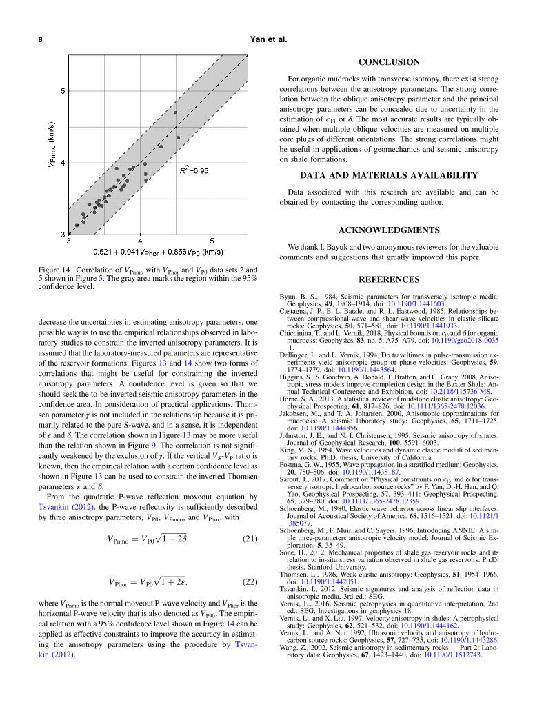
decrease the uncertainties in estimating anisotropy parameters, onepossible way is to use the empirical relationships observed in labo-ratory studies to constrain the inverted anisotropy parameters. It isassumed that the laboratory-measured parameters are representativeof the reservoir formations. Figures 13 and 14 show two forms ofcorrelations that might be useful for constraining the invertedanisotropy parameters. A confidence level is given so that weshould seek the to-be-inverted seismic anisotropy parameters in theconfidence area. In consideration of practical applications, Thom-sen parameter γ is not included in the relationship because it is pri-marily related to the pure S-wave, and in a sense, it is independentof ε and δ. The correlation shown in Figure 13 may be more usefulthan the relation shown in Figure 9. The correlation is not signifi-cantly weakened by the exclusion of γ. If the vertical VS-VP ratio isknown, then the empirical relation with a certain confidence level asshown in Figure 13 can be used to constrain the inverted Thomsenparameters ε and δ.From the quadratic P-wave reflection moveout equation by

Tsvankin (2012), the P-wave reflectivity is sufficiently describedby three anisotropy parameters, VP0, VPnmo, and VPhor, with

VPnmo ¼ VP0

ffiffiffiffiffiffiffiffiffiffiffiffiffi1þ 2δ

p; (21)

VPhor ¼ VP0

ffiffiffiffiffiffiffiffiffiffiffiffiffi1þ 2ε

p; (22)

where VPnmo is the normal moveout P-wave velocity and VPhor is thehorizontal P-wave velocity that is also denoted as VP90. The empiri-cal relation with a 95% confidence level shown in Figure 14 can beapplied as effective constraints to improve the accuracy in estimat-ing the anisotropy parameters using the procedure by Tsvan-kin (2012).

CONCLUSION

For organic mudrocks with transverse isotropy, there exist strongcorrelations between the anisotropy parameters. The strong corre-lation between the oblique anisotropy parameter and the principalanisotropy parameters can be concealed due to uncertainty in theestimation of c13 or δ. The most accurate results are typically ob-tained when multiple oblique velocities are measured on multiplecore plugs of different orientations. The strong correlations mightbe useful in applications of geomechanics and seismic anisotropyon shale formations.

DATA AND MATERIALS AVAILABILITY

Data associated with this research are available and can beobtained by contacting the corresponding author.

ACKNOWLEDGMENTS

We thank I. Bayuk and two anonymous reviewers for the valuablecomments and suggestions that greatly improved this paper.

REFERENCES

Byun, B. S., 1984, Seismic parameters for transversely isotropic media:Geophysics, 49, 1908–1914, doi: 10.1190/1.1441603.

Castagna, J. P., B. L. Batzle, and R. L. Eastwood, 1985, Relationships be-tween compressional-wave and shear-wave velocities in clastic silicaterocks: Geophysics, 50, 571–581, doi: 10.1190/1.1441933.

Chichinina, T., and L. Vernik, 2018, Physical bounds on c13 and δ for organicmudrocks: Geophysics, 83, no. 5, A75–A79, doi: 10.1190/geo2018-0035.1.

Dellinger, J., and L. Vernik, 1994, Do traveltimes in pulse-transmission ex-periments yield anisotropic group or phase velocities: Geophysics, 59,1774–1779, doi: 10.1190/1.1443564.

Higgins, S., S. Goodwin, A. Donald, T. Bratton, and G. Gracy, 2008, Aniso-tropic stress models improve completion design in the Baxter Shale: An-nual Technical Conference and Exhibition, doi: 10.2118/115736-MS.

Horne, S. A., 2013, A statistical review of mudstone elastic anisotropy: Geo-physical Prospecting, 61, 817–826, doi: 10.1111/1365-2478.12036.

Jakobsen, M., and T. A. Johansen, 2000, Anisotropic approximations formudrocks: A seismic laboratory study: Geophysics, 65, 1711–1725,doi: 10.1190/1.1444856.

Johnston, J. E., and N. I. Christensen, 1995, Seismic anisotropy of shales:Journal of Geophysical Research, 100, 5591–6003.

King, M. S., 1964, Wave velocities and dynamic elastic moduli of sedimen-tary rocks: Ph.D. thesis, University of California.

Postma, G. W., 1955, Wave propagation in a stratified medium: Geophysics,20, 780–806, doi: 10.1190/1.1438187.

Sarout, J., 2017, Comment on “Physical constraints on c13 and δ for trans-versely isotropic hydrocarbon source rocks” by F. Yan, D.-H. Han, and Q.Yao, Geophysical Prospecting, 57, 393–411: Geophysical Prospecting,65, 379–380, doi: 10.1111/1365-2478.12359.

Schoenberg, M., 1980, Elastic wave behavior across linear slip interfaces:Journal of Acoustical Society of America, 68, 1516–1521, doi: 10.1121/1.385077.

Schoenberg, M., F. Muir, and C. Sayers, 1996, Introducing ANNIE: A sim-ple three-parameters anisotropic velocity model: Journal of Seismic Ex-ploration, 5, 35–49.

Sone, H., 2012, Mechanical properties of shale gas reservoir rocks and itsrelation to in-situ stress variation observed in shale gas reservoirs: Ph.D.thesis, Stanford University.

Thomsen, L., 1986, Weak elastic anisotropy: Geophysics, 51, 1954–1966,doi: 10.1190/1.1442051.

Tsvankin, I., 2012, Seismic signatures and analysis of reflection data inanisotropic media, 3rd ed.: SEG.

Vernik, L., 2016, Seismic petrophysics in quantitative interpretation, 2nded.: SEG, Investigations in geophysics 18.

Vernik, L., and X. Liu, 1997, Velocity anisotropy in shales: A petrophysicalstudy: Geophysics, 62, 521–532, doi: 10.1190/1.1444162.

Vernik, L., and A. Nur, 1992, Ultrasonic velocity and anisotropy of hydro-carbon source rocks: Geophysics, 57, 727–735, doi: 10.1190/1.1443286.

Wang, Z., 2002, Seismic anisotropy in sedimentary rocks — Part 2: Labo-ratory data: Geophysics, 67, 1423–1440, doi: 10.1190/1.1512743.

Figure 14. Correlation of VPnmo with VPhor and VP0 data sets 2 and5 shown in Figure 5. The gray area marks the region within the 95%confidence level.

8 Yan et al.

Yan, F., and D.-H. Han, 2018, Accuracy and sensitivity analysis on seismicanisotropy parameter estimation: Journal of Geophysics and Engineering,15, 539–553, doi: 10.1088/1742-2140/aa93b1.

Yan, F., D.-H. Han, and X.-L. Chen, 2018, Practical and robust experimentaldetermination of c13 and Thomsen parameter δ: Geophysical Prospecting,66, 354–365, doi: 10.1111/1365-2478.12514.

Yan, F., D.-H. Han, X.-L. Chen, J. Ren, and Y. Wang, 2017, Comparisonof dynamic and static bulk moduli of reservoir rocks: 87th Annual

International Meeting, SEG, Expanded Abstracts, 3711–3715, doi: 10.1190/segam2017-17664075.1.

Yan, F., D.-H. Han, and Q. Yao, 2012, Oil shale anisotropy measurement andsensitivity analysis: 82nd Annual International Meeting, SEG, ExpandedAbstracts, doi: 10.1190/segam2012-1106.1.

Yan, F., D.-H. Han, and Q. Yao, 2016, Physical constrains on c13 and δ fortransversely isotropic hydrocarbon source rocks: Geophysical Prospec-ting, 64, 1524–1536, doi: 10.1111/1365-2478.12265.

Correlations between seismic anisotropy parameters 9