determination of seismic anisotropy parameters from

DETERMINATION OF SEISMIC ANISOTROPY PARAMETERS FROM

MULTICOMPONENT VERTICAL SEISMIC PROFILES

FOR IMPROVED SEISMIC IMAGING AND

RESERVOIR CHARACTERIZATION

by

Naser Tamimi

c© Copyright by Naser Tamimi, 2015

All Rights Reserved

A thesis submitted to the Faculty and the Board of Trustees of the Colorado School

of Mines in partial fulfillment of the requirements for the degree of Doctor of Philosophy

(Geophysics).

Golden, Colorado

Date

Signed:Naser Tamimi

Signed:Dr. Thomas L. Davis

Thesis Advisor

Golden, Colorado

Date

Signed:Dr. Terence K. Young

Professor and HeadDepartment of Geophysics

ii

ABSTRACT

Multicomponent vertical seismic profile (VSP) data can be used to determine seismic

anisotropy more accurately. First, I modify the slowness-polarization method by includ-

ing both P- and SV-wave data for estimating the parameters δ and η of VTI (transversely

isotropic with vertical symmetry axis) media. Then I apply the technique to a multicompo-

nent VSP dataset from the Wattenberg Field in Colorado, USA.

The importance of the derived anisotropic velocity model from the joint P- and SV-

wave slowness-polarization method for reservoir characterization at the Wells Ranch VSP

area is: 1) identifying the possible existence of open fracture networks in the Niobrara

Formation at the VSP well location, 2) improving the quality of the Niobrara Formation

image which is vital for future drilling programs,, 3) accurately depicting the structure in

the well vicinity and finally 4) determining elastic properties of the Niobrara reservoir. To

identify the existence of open fracture networks, azimuthal AVO response of top of the

Niobrara Formation at the VSP well is analyzed. To correct the azimuthal AVO response

for propagation phenomena, using the anisotropic velocity model from the joint slowness-

polarization method, I modified the moveout-based anisotropic spreading correction (MASC)

technique for the VSP data.

The azimuthal AVO analysis shows very weak azimuthal anisotropy at the top of Niobrara

Formation near the VSP well. This result indicates the lack of open natural fractures at the

Niobrara Formation in this area and explains the low production associated with the well. In

addition, I used the anisotropic velocity model obtained from the joint slowness-polarization

method to build a 2D VSP image. Comparing the final VSP images using the isotropic

and anisotropic velocity models with well data shows that the anisotropic image is more

accurately depicted and if inverted would give more robust elastic parameter definition.

iii

TABLE OF CONTENTS

ABSTRACT . . . . . . . . . . . . . . . . . . . . . . . . . . . . . . . . . . . . . . . . . iii

LIST OF FIGURES . . . . . . . . . . . . . . . . . . . . . . . . . . . . . . . . . . . . . vii

LIST OF TABLES . . . . . . . . . . . . . . . . . . . . . . . . . . . . . . . . . . . . . . xiv

LIST OF SYMBOLS . . . . . . . . . . . . . . . . . . . . . . . . . . . . . . . . . . . . . xv

LIST OF ABBREVIATIONS . . . . . . . . . . . . . . . . . . . . . . . . . . . . . . . xvii

ACKNOWLEDGMENTS . . . . . . . . . . . . . . . . . . . . . . . . . . . . . . . . . xviii

DEDICATION . . . . . . . . . . . . . . . . . . . . . . . . . . . . . . . . . . . . . . . . xx

CHAPTER 1 INTRODUCTION . . . . . . . . . . . . . . . . . . . . . . . . . . . . . . . 1

1.1 Brief Theory of Seismic Anisotropy . . . . . . . . . . . . . . . . . . . . . . . . . 2

1.2 Research Objectives and Values . . . . . . . . . . . . . . . . . . . . . . . . . . . 5

1.3 Case Study . . . . . . . . . . . . . . . . . . . . . . . . . . . . . . . . . . . . . . 6

1.4 Data . . . . . . . . . . . . . . . . . . . . . . . . . . . . . . . . . . . . . . . . . 10

1.5 Thesis Layout . . . . . . . . . . . . . . . . . . . . . . . . . . . . . . . . . . . . 13

CHAPTER 2 USING P- AND S-WAVE VSP DATA FOR ESTIMATING LOCALSEISMIC ANISOTROPY PARAMETERS. . . . . . . . . . . . . . . . . 15

2.1 Introduction . . . . . . . . . . . . . . . . . . . . . . . . . . . . . . . . . . . . . 15

2.2 Theory of Local Anisotropy Estimation Using VSP Data . . . . . . . . . . . . 16

2.2.1 Slowness Method . . . . . . . . . . . . . . . . . . . . . . . . . . . . . . 17

2.2.2 Slowness-Polarization Method . . . . . . . . . . . . . . . . . . . . . . . 17

2.3 Methodology . . . . . . . . . . . . . . . . . . . . . . . . . . . . . . . . . . . . 25

iv

2.4 9C Synthetic VSP Data . . . . . . . . . . . . . . . . . . . . . . . . . . . . . . 28

2.5 Results and Discussion . . . . . . . . . . . . . . . . . . . . . . . . . . . . . . . 30

2.6 Conclusions . . . . . . . . . . . . . . . . . . . . . . . . . . . . . . . . . . . . . 36

CHAPTER 3 ESTIMATING LOCAL SEISMIC ANISOTROPY PARAMETERSUSING P- AND SV-WAVE VERTICAL SLOWNESSCOMPONENTS AND POLARIZATION ANGLES AT WELLSRANCH AREA, WATTENBERG FIELD, COLORADO. . . . . . . . . 42

3.1 Introduction . . . . . . . . . . . . . . . . . . . . . . . . . . . . . . . . . . . . . 42

3.2 Wattenberg Field Geology and Wells Ranch VSP Data . . . . . . . . . . . . . 43

3.2.1 3D-9C VSP Data Acquisition . . . . . . . . . . . . . . . . . . . . . . . 44

3.3 Data Analysis and Processing . . . . . . . . . . . . . . . . . . . . . . . . . . . 44


3.5 Conclusions . . . . . . . . . . . . . . . . . . . . . . . . . . . . . . . . . . . . . 54

CHAPTER 4 PRESTACK WAVEFORM INVERSION OF MULTICOMPONENTVSP DATA FOR ESTIMATING ORTHORHOMBIC ANISOTROPYPARAMETERS AT THE WELLS RANCH AREA, WATTENBERGFIELD, COLORADO . . . . . . . . . . . . . . . . . . . . . . . . . . . . 58

4.1 Introduction . . . . . . . . . . . . . . . . . . . . . . . . . . . . . . . . . . . . . 58

4.2 Methodology . . . . . . . . . . . . . . . . . . . . . . . . . . . . . . . . . . . . 59

4.3 Review of the Dataset . . . . . . . . . . . . . . . . . . . . . . . . . . . . . . . 61

4.4 Model Description . . . . . . . . . . . . . . . . . . . . . . . . . . . . . . . . . 62


4.6 Conclusions . . . . . . . . . . . . . . . . . . . . . . . . . . . . . . . . . . . . . 64

CHAPTER 5 APPLICATIONS OF THE ANISOTROPIC VELOCITY MODELOBTAINED FROM JOINT SLOWNESS-POLARIZATIONMETHOD IN PRE- AND POST-STACK VSP DATA ANALYSES . . . 69

v

5.1 Introduction . . . . . . . . . . . . . . . . . . . . . . . . . . . . . . . . . . . . . 69

5.2 Theory of MASC . . . . . . . . . . . . . . . . . . . . . . . . . . . . . . . . . . 71

5.3 Modifying MASC for VSP Data . . . . . . . . . . . . . . . . . . . . . . . . . . 72

5.4 Applying MASC to VSP Data . . . . . . . . . . . . . . . . . . . . . . . . . . . 75


5.6 Conclusions . . . . . . . . . . . . . . . . . . . . . . . . . . . . . . . . . . . . . 84

CHAPTER 6 CONCLUSIONS AND RECOMMENDATIONS . . . . . . . . . . . . . . 90

6.1 Conclusions . . . . . . . . . . . . . . . . . . . . . . . . . . . . . . . . . . . . . 90

6.2 Recommendations . . . . . . . . . . . . . . . . . . . . . . . . . . . . . . . . . . 91

REFERENCES CITED . . . . . . . . . . . . . . . . . . . . . . . . . . . . . . . . . . . 93

APPENDIX - WEAK ANISOTROPY APPROXIMATION OF SV-WAVEVERTICAL SLOWNESS AS A FUNCTION OF POLARIZATIONANGLE IN A VTI MEDIUM . . . . . . . . . . . . . . . . . . . . . . . . 99

vi

LIST OF FIGURES

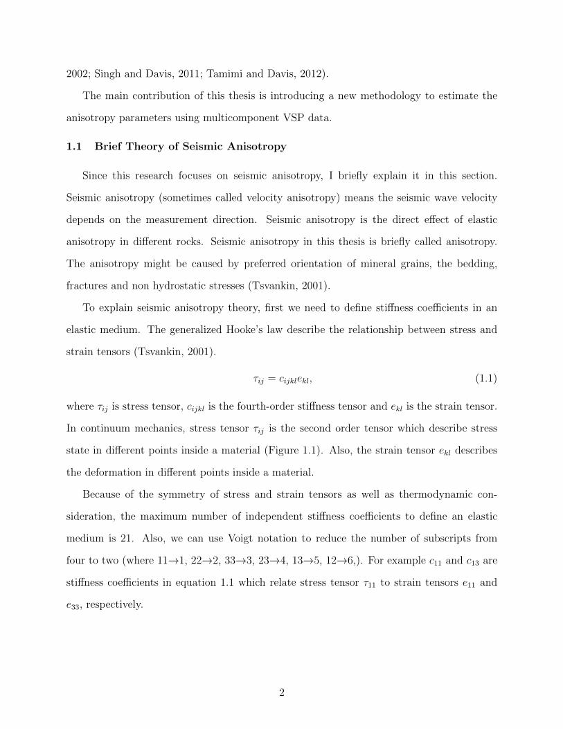
Figure 1.1 Stress tensor τij in a 3D space. . . . . . . . . . . . . . . . . . . . . . . . . . 3

Figure 1.2 Transversely isotropic medium with vertical symmetry axis (VTI). . . . . . 4

Figure 1.3 P-wave wavefront (solid white) in a VTI medium with ε ≈0.1 andδ ≈-0.1. The isotropic wavefront with the velocity VP0 is marked by thedashed white line . . . . . . . . . . . . . . . . . . . . . . . . . . . . . . . . . 5

Figure 1.4 Map of important US lower 48 states shale plays (source:www.cleanskies.org). . . . . . . . . . . . . . . . . . . . . . . . . . . . . . . 7

Figure 1.5 Total oil (top) and natural gas (bottom) production from sixunconventional plays in the US in 2013 and 2014 . . . . . . . . . . . . . . . 8

Figure 1.6 New-well oil (top) and natural gas (bottom) production per rig from sixunconventional plays in the US in 2013 and 2014 . . . . . . . . . . . . . . . 9

Figure 1.7 Monthly oil and gas production, number of production wells andaverage daily production for each well in the Wattenberg Field (source:Colorado Oil and Gas Conservation Commission). . . . . . . . . . . . . . 11

Figure 1.8 Wattenberg Field stratigraphy and deposition history. The left panelhighlights plays in the field and their types. The red and green markerson the left panel show gas and oil producing layers, respectively . . . . . . 12

Figure 1.9 Cross section (a) and map (b) views of VSP survey from Wells Rancharea, Wattenberg Field, Colorado. . . . . . . . . . . . . . . . . . . . . . . 12

Figure 1.10 A display of a random shot location from Wells Ranch area 9C VSPdata after receiver reorientation. . . . . . . . . . . . . . . . . . . . . . . . 13

Figure 2.1 Exact vertical slowness (q) versus polarization angle (ψ) for the P- andSV-waves (solid curves) and their weak-anisotropy approximations(dashed curves) for four different VTI models. For all models,VP0=2420 m/s and VS0=1400 m/s (the example values are the same thevalues used by for analyzing weak-anisotropy approximation ofSV-wave velocity in terms of phase angle). . . . . . . . . . . . . . . . . . 21

vii

Figure 2.2 Magnitudes of δ- and η-term coefficients in equation 2.15 for f0=1.5normalized by the isotropic term (adapted from V. Grechka, personalcommunication, 20 October 2014). . . . . . . . . . . . . . . . . . . . . . . 22

Figure 2.3 Color map of |δ|-term coefficient minus |η|-term coefficient for a rangeof VP0/VS0 normalized by the isotropic term. Positive values showhigher δ-term coefficient compared to η-term coefficient and dashedwhite lines show the boundaries for the positive values. The solid whiteline shows where η-term goes zero and the δ-term dominates qSV (ψSV ). . 23

Figure 2.4 Condition number calculated for P- and SV-wave WAA (equations 2.10and 2.11) for different VP0/VS0 ratio. Larger condition number indicatesthat a small error in the data cause a large error in the estimatedparameters. . . . . . . . . . . . . . . . . . . . . . . . . . . . . . . . . . . 24

Figure 2.5 For a range of δ (0.00 ≤ δ ≤ 0.30) and η (0.00 ≤ η ≤ 0.30) values, P-and SV-wave vertical slownesses versus their polarization angles areplotted. . . . . . . . . . . . . . . . . . . . . . . . . . . . . . . . . . . . . . 25

Figure 2.6 To measure the variation of P- and SV-wave curves in differentanisotropic media, the slowness-polarization curves of more than 30000different anisotropy cases were compared using the visual l2 measure,also called dv distance, for P- and SV-wave separately (Figure 2.6).SV-wave data show higher dv distance, which means more variation fordifferent anisotropic media. . . . . . . . . . . . . . . . . . . . . . . . . . . 26

Figure 2.7 To understand the effect of the measurement error on the final results, Iestimated δ and η parameters for three different scenarios. Scenario 1)VP0 = VS0 = ±0%, qP = ±2%, qSV = ±2%, ψP = ±5◦ and ψSV = ±5◦.Scenario 2) VP0 = VS0 = ±0%, qP = ±2%, qSV = ±4%, ψP = ±5◦ andψSV = ±10◦. Scenario 3) VP0 = VS0 = ±2%, qP = ±2%, qSV = ±4%,ψP = ±5◦ and ψSV = ±10◦. . . . . . . . . . . . . . . . . . . . . . . . . . . 27

Figure 2.8 2D 9C VSP data have been generated from a model with fourhorizontal layers. Three layers are VTI and the shallowest layer isisotropic. The density for all layers is constant and equal to 2.28g/cc.26 geophones record data from 1400m to 2900m (60m distance betweentwo geophones) in the VSP well. Both horizontal and vertical sourcesshoot every 150m from 100m up to 6100m away from the VSP well. . . . 29

Figure 2.9 Vertical component of recorded data using vertical seismic source isshown on top and radial component of horizontal source is shown below. . 30

viii

Figure 2.10 Linearity of the particle motion for P-, pure SV- and convertedSV-wave. 1 is perfectly linear particle motion and 0 is circular particlemotion. . . . . . . . . . . . . . . . . . . . . . . . . . . . . . . . . . . . . . 31

Figure 2.11 Left plots, (a) and (c), are results using both P- and SV-wave data, andright plots, (b) and (d), came from fitting models to P-wave data only.(a) and (b) depict the best fitted model (dashed lines) with data(circles) for receiver group number 10, which consists of 3 receivers,centered at a depth of 2000 m. The weighted SSE (sum of squarederrors) maps in Figures (c) and (d) show the difference between modelswith different δ and η pairs and the data. Circles on plots (b) and (d)show the real parameters and crosses locate estimated δ and ηparameters. . . . . . . . . . . . . . . . . . . . . . . . . . . . . . . . . . . 32

Figure 2.12 Estimated δ and η logs using P-wave data only (dotted lines) and jointP- and SV-wave (solid lines) techniques. The actual δ and η values(using a 3-geophones average window) is shown with light thick lines. . . 33

Figure 2.13 Error maps show the difference between data from receiver no. 10 andmodels with different δ and η pairs. The error maps were calculatedusing models with ±2% error and without error in VP0 and VS0calculation. The minimum error in each map locates the estimatedparameters and shown with cross markers. The real parameters areshown with circles on the maps. . . . . . . . . . . . . . . . . . . . . . . . 34

Figure 2.14 Sensitivity of final results to WP and WSV values. Error maps show thedifference between data from receiver no. 18 and models with differentδ and η pairs. The error maps were calculated using models withdifferent WP and WSV values. The minimum error in each map locatesthe estimated parameters and shown with cross markers. The realparameters are shown with circles on the maps. . . . . . . . . . . . . . . . 37

Figure 2.15 Summary of error of estimation for different WP and WSV combinationsfor entire VSP interval. . . . . . . . . . . . . . . . . . . . . . . . . . . . . 38

Figure 2.16 Estimated δ and η logs using P- and converted SV-wave data (dottedlines) vs. estimated parameters from P- and pure SV-wave (solid lines).The actual δ and η values (using a 3-geophones average window) isshown with light thick lines. . . . . . . . . . . . . . . . . . . . . . . . . . 39

Figure 2.17 Polarization angle of pure SV- and converted SV-wave data used in thejoint inversion. . . . . . . . . . . . . . . . . . . . . . . . . . . . . . . . . . 40

ix

Figure 2.18 Squared error of estimated parameters for P-wave data only, joint P-and pure SV-wave data and joint P- and converted SV-wave dataapproaches. . . . . . . . . . . . . . . . . . . . . . . . . . . . . . . . . . . 41

Figure 3.1 The Wells Ranch area in the Wattenberg field, Weld county, Colorado. . . 43

Figure 3.2 Generalized stratigraphic column of Cretaceous formations across theWattenberg Field. Dots represent time periods of wrench faultmovement . Most of the VSP receivers in this study are located in thePierre Shale Formation. . . . . . . . . . . . . . . . . . . . . . . . . . . . . 44

Figure 3.3 VSP acquisition cross section (a) and map (b) for the 9C VSP survey inthe Wells Ranch area. . . . . . . . . . . . . . . . . . . . . . . . . . . . . 45

Figure 3.4 Azimuth of one of the symmetry planes from the best-fittednon-hyperbolic surfaces on first break arrivals for each geophone. . . . . . 46

Figure 3.5 Source statics map for the Wells Ranch area VSP survey. The color barshows the calculated source statics in ms. . . . . . . . . . . . . . . . . . . 47

Figure 3.6 Ratio of S-wave RMS amplitude of diagonal components to off-diagonalcomponents for number of source locations with offset of 240-460m. . . . 48

Figure 3.7 Ratio of S-wave RMS amplitude of diagonal components to off-diagonalcomponents for 6 different source locations with offset of 609.6m andradial component azimuth varying from 85 degrees to 160 degrees. Thehighest ratio shows the azimuth of one of symmetry planes. . . . . . . . . 48

Figure 3.8 Anisotropy azimuth from the dipole sonic log for the depth interval of1500-2000 m. The log was acquired from a nearby well (1.82 km awayfrom the VSP well). . . . . . . . . . . . . . . . . . . . . . . . . . . . . . . 49

Figure 3.9 Top figures are two examples from NE line and the two bottom figuresare from SE line. Blue circles and red crosses are P- and SV-wave data,respectively. Dashed blue and red lines are best-fit P- and SV-wavemodels. . . . . . . . . . . . . . . . . . . . . . . . . . . . . . . . . . . . . 51

Figure 3.10 Estimated δ, η, VP0 and VS0 for NE symmetry plane. Gamma ray logon left is for the purpose of comparison. . . . . . . . . . . . . . . . . . . . 52

Figure 3.11 Estimated δ, η, VP0 and VS0 for SE symmetry plane. Gamma ray log onleft is for the purpose of comparison. . . . . . . . . . . . . . . . . . . . . 53

Figure 3.12 The correlation between estimated anisotropy parameters and well logs. . 54

x

Figure 3.13 The estimated η parameter in the SE symmetry plane is compared withthe deep resistivity log (left) and the density log (right). . . . . . . . . . . 55

Figure 3.14 (a) water-clay composite; (b) clay sheets and clay-bound water; (c)water-clay polycrystal. Figures (a) and (c) are taken from . . . . . . . . 56

Figure 3.15 Estimating anisotropy parameters, δ and η, for NE symmetry plane.Solid lines show the results by using P-wave data only and dotted linesare results of using both P- and SV-wave data, simultaneously. . . . . . . 57

Figure 4.1 An example of ranking Pareto-optimal fronts. The entire solutions areranked into different Pareto-optimal front classes based on theirdominance levels. . . . . . . . . . . . . . . . . . . . . . . . . . . . . . . . 60

Figure 4.2 Proposed parallel NSGA II workflow by . . . . . . . . . . . . . . . . . . . 62

Figure 4.3 VSP acquisition cross section (a) and map (b) for the 9C VSP survey inthe Wells Ranch area. . . . . . . . . . . . . . . . . . . . . . . . . . . . . 63

Figure 4.4 Waveform inversion results after 500 generations. The 3C prestack data(from vertical sources) were inverted for orthorhombic anisotropicparameters: ε(1), ε(2), γ(1) and γ(2). Red lines represent the waveforminversion results. Black lines show anisotropy parameters (smoothedwith a sliding average window) using the joint P- and SV-waveslowness-polarization method. . . . . . . . . . . . . . . . . . . . . . . . . 66

Figure 4.5 Waveform inversion results after 500 generations. The 3C prestack data(from vertical sources) were inverted for orthorhombic anisotropicparameters: δ(1), δ(2), δ(3) and symmetry plane azimuth. Red linesrepresent the waveform inversion results. Black lines show anisotropyparameters (smoothed with a sliding average window) using the jointP- and SV-wave slowness-polarization method. . . . . . . . . . . . . . . . 67

Figure 4.6 Estimated orthorhombic anisotropy parameters, δ(1),(2), ε(1),(2) and γ(S)

in 200m depth interval around the target. . . . . . . . . . . . . . . . . . . 68

Figure 5.1 Schematic VSP geometry for a laterally homogeneous horizontal layer.S and R are source and receiver in a VSP acquisition geometry, R′ ispseudo-receiver after tracing the ray SR to the surface. S ′ is apseudo-source for imaginary S ′RR′ reflection. . . . . . . . . . . . . . . . . 73

Figure 5.2 The effective moveout parameters were estimated by fitting thebest-fitted nonhyperbolic moveout surface on the first break arrivalsmultiplied by two. . . . . . . . . . . . . . . . . . . . . . . . . . . . . . . . 76

xi

Figure 5.3 Traveltime difference maps, ∆T = Tdata − Tmodel, where estimatedtraveltime from effective moveout parameters is Tmodel), and the actualtraveltime is Tdata. . . . . . . . . . . . . . . . . . . . . . . . . . . . . . . . 77

Figure 5.4 Anisotropic velocity models for two symmetry planes, NE and SEplanes, obtained from the joint P- and SV-wave slowness-polarizationmethod. . . . . . . . . . . . . . . . . . . . . . . . . . . . . . . . . . . . . 78

Figure 5.5 L factor is calculated for different source and receiver pairs of the VSPsurvey in SE (a) and NE (b) directions after ray tracing using ananisotropic velocity model. For the purpose of comparison, (c) showsthe results for NE line using an isotropic velocity model. . . . . . . . . . . 79

Figure 5.6 (a) Estimated interval QP for the entire VSP array (solid black line)and effective QP for the Niobrara Formation (dashed orange line). Tocalculate the effective QP , amplitude spectrums of the vertical sourcesweep and the last receiver in the VSP array were used (b). Plot (c)shows the best linear equation fitted to the amplitude ratio of thesource sweep and the last receiver. . . . . . . . . . . . . . . . . . . . . . . 80

Figure 5.7 VSP shot gather example from receiver no. 50 after wavefieldseparation and separating reflection data (upgoing waves) fromdowngoing data. Left and right panels show the NE and SE lines,respectively. The red arrows depict the top of Niobrara reflection thatis around 730ms at the nearest offset. . . . . . . . . . . . . . . . . . . . . 81

Figure 5.8 Summary of the VSP processing workflow. . . . . . . . . . . . . . . . . . 86

Figure 5.9 Normalized amplitude from top of the Niobrara Formation versussin2(i) where i is the incidence angle. The blue and red lines representthe AVO curves in NE and SE directions. The dotted black line is theisotropic AVO model calculated using well log data. The green line is aVTI AVO model with the same values as the isotropic model andassuming ∆δ = −0.16 and ∆ε = 0.17. The magenta curve in the lowerplot depicts amplitude difference between SE and NE lines (i.e.AmplitudeSE − AmplitudeNE) . . . . . . . . . . . . . . . . . . . . . . . . 87

Figure 5.10 Coherency map from the surface seismic data at the Wells Ranch area(internal study by Noble Energy Inc.). . . . . . . . . . . . . . . . . . . . . 88

Figure 5.11 VSP images of the Niobrara Formation using anisotropic velocity model(top) and isotropic velocity model (bottom). . . . . . . . . . . . . . . . . 89

xii

Figure A.1 Diagram of phase angle (θ), P-wave polarization angle (ψP ), SV-wavepolarization angle (ψSV ) and the angle between SV-wave polarizationvector and the horizontal axis (νSV ) in a VTI medium. . . . . . . . . . 100

xiii

LIST OF TABLES

Table 1.1 Wells Ranch area VSP survey acquisition parameters. . . . . . . . . . . . . 10

Table 4.1 Model constraints. . . . . . . . . . . . . . . . . . . . . . . . . . . . . . . . . 64

xiv

LIST OF SYMBOLS

Anellipticity parameter . . . . . . . . . . . . . . . . . . . . . . . . . . . . . . . . . . . . . η

Azimuthal polarization angle . . . . . . . . . . . . . . . . . . . . . . . . . . . . . . . . φ

Bulk density . . . . . . . . . . . . . . . . . . . . . . . . . . . . . . . . . . . . . . . . . . ρ

Christoffel Matrix . . . . . . . . . . . . . . . . . . . . . . . . . . . . . . . . . . . . . . Gij

Data domain . . . . . . . . . . . . . . . . . . . . . . . . . . . . . . . . . . . . . . . . . . d

Excitation time . . . . . . . . . . . . . . . . . . . . . . . . . . . . . . . . . . . . . . . . t0

Green’s function . . . . . . . . . . . . . . . . . . . . . . . . . . . . . . . . . . . . . . Gin

Kronecker delta . . . . . . . . . . . . . . . . . . . . . . . . . . . . . . . . . . . . . . . . δij

Model domain . . . . . . . . . . . . . . . . . . . . . . . . . . . . . . . . . . . . . . . . . m

NMO (Normal Moveout) velocity . . . . . . . . . . . . . . . . . . . . . . . . . . . . . Vnmo

Objective function . . . . . . . . . . . . . . . . . . . . . . . . . . . . . . . . . . . . E(m)

P-wave data weight . . . . . . . . . . . . . . . . . . . . . . . . . . . . . . . . . . . . . WP

P-wave vertical velocity . . . . . . . . . . . . . . . . . . . . . . . . . . . . . . . . . . VP0

Phase velocity . . . . . . . . . . . . . . . . . . . . . . . . . . . . . . . . . . . . . . . . . V

Polar phase angle . . . . . . . . . . . . . . . . . . . . . . . . . . . . . . . . . . . . . . . . θ

Polar polarization angle . . . . . . . . . . . . . . . . . . . . . . . . . . . . . . . . . . . ψ

Polarization vector . . . . . . . . . . . . . . . . . . . . . . . . . . . . . . . . . . . . . . U

Pseudo-receiver . . . . . . . . . . . . . . . . . . . . . . . . . . . . . . . . . . . . . . . . R′

Pseudo-source . . . . . . . . . . . . . . . . . . . . . . . . . . . . . . . . . . . . . . . . . S ′

Receiver . . . . . . . . . . . . . . . . . . . . . . . . . . . . . . . . . . . . . . . . . . . . R

xv

Recording time . . . . . . . . . . . . . . . . . . . . . . . . . . . . . . . . . . . . . . . . . t

Reflection coefficient in [x,z] plane . . . . . . . . . . . . . . . . . . . . . . . . . . . R[x,z]

Relative geometrical spreading . . . . . . . . . . . . . . . . . . . . . . . . . . . . . . . L

SV-wave data weight . . . . . . . . . . . . . . . . . . . . . . . . . . . . . . . . . . . . WSV

Shear-wave splitting parameter . . . . . . . . . . . . . . . . . . . . . . . . . . . . . . . γS

Slowness vector . . . . . . . . . . . . . . . . . . . . . . . . . . . . . . . . . . . . . . . . p

Source . . . . . . . . . . . . . . . . . . . . . . . . . . . . . . . . . . . . . . . . . . . . . S

Source-receiver azimuth . . . . . . . . . . . . . . . . . . . . . . . . . . . . . . . . . . . α

Stiffness coefficient . . . . . . . . . . . . . . . . . . . . . . . . . . . . . . . . . . . . . cijkl

Thomsen anisotropy parameter . . . . . . . . . . . . . . . . . . . . . . . . . . . . . . . . ε

Thomsen anisotropy parameter . . . . . . . . . . . . . . . . . . . . . . . . . . . . . . . . δ

Traveltime . . . . . . . . . . . . . . . . . . . . . . . . . . . . . . . . . . . . . . . . . . . T

Unit wavefront-normal vector . . . . . . . . . . . . . . . . . . . . . . . . . . . . . . . . n

Vertical slowness component . . . . . . . . . . . . . . . . . . . . . . . . . . . . . . . . . . q

Vertical velocity of S-wave polarized in x1-direction . . . . . . . . . . . . . . . . . . . VS0

xvi

LIST OF ABBREVIATIONS

Amplitude Variation with Azimuth . . . . . . . . . . . . . . . . . . . . . . . . . . . AVAZ

Amplitude Variation with Offset . . . . . . . . . . . . . . . . . . . . . . . . . . . . AVO

Full Waveform Inversion . . . . . . . . . . . . . . . . . . . . . . . . . . . . . . . . . . FWI

Horizontal Transverse Isotropy . . . . . . . . . . . . . . . . . . . . . . . . . . . . . . HTI

In plane-polarized shear wave . . . . . . . . . . . . . . . . . . . . . . . . . . . . SV-wave

Moveout-based Anisotropic Spreading Correction . . . . . . . . . . . . . . . . . . MASC

Multiobjective Evolutionary Algorithm . . . . . . . . . . . . . . . . . . . . . . . . MOEA

Nine Components . . . . . . . . . . . . . . . . . . . . . . . . . . . . . . . . . . . . . . . 9C

Non-dominated Sorting Genetic Algorithm II . . . . . . . . . . . . . . . . . . . NSGA II

Normal Moveout . . . . . . . . . . . . . . . . . . . . . . . . . . . . . . . . . . . . . NMO

Primary or compressional wave . . . . . . . . . . . . . . . . . . . . . . . . . . . . P-wave

Reservoir Characterization Project . . . . . . . . . . . . . . . . . . . . . . . . . . . . RCP

Root Mean Square . . . . . . . . . . . . . . . . . . . . . . . . . . . . . . . . . . . . RMS

Secondary or shear wave . . . . . . . . . . . . . . . . . . . . . . . . . . . . . . . . S-wave

Society of Exploration Geophysicists . . . . . . . . . . . . . . . . . . . . . . . . . . . SEG

Sum of Squared Error . . . . . . . . . . . . . . . . . . . . . . . . . . . . . . . . . . . SSE

Tilted Transverse Isotropy . . . . . . . . . . . . . . . . . . . . . . . . . . . . . . . . . TTI

Vertical Seismic Profiling . . . . . . . . . . . . . . . . . . . . . . . . . . . . . . . . . . VSP

Vertical Transverse Isotropy . . . . . . . . . . . . . . . . . . . . . . . . . . . . . . . . VTI

Weak-Anisotropy Approximation . . . . . . . . . . . . . . . . . . . . . . . . . . . . WAA

xvii

ACKNOWLEDGMENTS

First, I thank my advisor, Professor Tom Davis, for his guidance, and generous support

during my PhD. I would like to thank him for encouraging my research and supporting me

to achieve academic and social goals. I am also grateful to Dr. Bob Benson for his technical

support and guidance. I cannot express enough thanks to Professor Ilya Tsvankin, Dr Bruce

Mattocks and Dr Vladimir Grechka for their scientific and technical advice. I am grateful to

Professor Hossein Kazemi, my Minor Degree Advisor, for his valuable comments too. I also

want to thank Professor Roel Snieder, Professor Mike Batzle and Professor John Curtis for

allowing me to find my research direction through their advice.

I would like to acknowledge Damon Parker, Dan Pearce, Jeffrey Grana and Noble Energy

Inc. for giving permission to use the Wells Ranch area VSP data for this study and their

constant support. Also, Rich Van Dok, Brian Fuller and Sigma Cubed Inc. provided the

softwares and support for doing this research. Mike O’Brien, Allied Geophysics Inc., gener-

ously built synthetic VSP data for my research, and I can not thank him enough. I thank

Tao Li and Dr Mallick from University of Wyoming who accepted my offer for a research

collaboration and shared their experiences with me. I am also grateful to Whiting Petroleum

Corporation, the previous operator of the Postle Field, for providing VSP data for the early

stages of my PhD research.

I am indebted to Dr. Aaron Wandler, Dr. Paritosh Singh, Milad Saidian, Mohsen Minaei

and the Reservoir Characterization Project students and staff for their scientific and non-

scientific support. In addition, I want to thank Dr Terry Young, head of the Department of

Geophysics, Michelle Szobody, Program Assistant, and Alyda Morosco, Assistant Director

at CSM International Student Office, who helped me during these years.

My father, Abdolreza, is not only my father but my great teacher, and I can not thank

him enough. I want to thank my mother, Shahla, who has been source of love and emotions in

xviii

my life. Most importantly, I would like to thank my wife, Shirin, for her love and inspiration.

I could not finish this journey without her generous support and encouragement.

xix

To my beloved country, IRAN

for a peaceful future ...

xx

CHAPTER 1

INTRODUCTION

It has been more than a century since anisotropy entered seismology. Although seismic

anisotropy was considered as an unwanted complication for many geophysical studies in

early days, a number of research projects in the 1970s and 1980s (e.g. Crampin, 1978, 1981,

1983, 1987; Gupta, 1973a,b) viewed anisotropy as an opportunity for geophysical studies

(Helbig and Thomsen, 2005). Ignoring anisotropy in seismic data processing causes serious

problems such as unfocused migrated images, misplaced reflectors and amplitude distortions

(Tsvankin and Grechka, 2011). Seismic anisotropy analysis improves our understanding of

the subsurface properties, such as natural fracture characterization and identifying subsurface

stress regime for better reservoir characterization and seismic data interpretation. One of the

challenges when accounting for seismic anisotropy is a lack of robust techniques for extracting

subsurface anisotropy properties (Helbig and Thomsen, 2005; Tsvankin, 2001; Tsvankin and

Grechka, 2011). This thesis focuses on new and robust methodologies to extract subsurface

anisotropic properties using multicomponent vertical seismic profile (VSP) data.

The advantage of VSP data is recording in-situ wave parameters, such as slowness and

polarization in depth. In addition, higher data quality and wide data aperture make VSP

data a promising tool for better characterization of subsurface anisotropy when compared to

surface seismic data. The VSP data are further enhanced by using multicomponent technol-

ogy. The mutlicomponent seismic technology expands the wavefield to include converted and

non-converted shear waves which can provide unique and additional rock, fluid and litholog-

ical information (Hardage et al., 2011). The Reservoir Characterization Project (RCP) at

Colorado School of Mines is one of a few academic research groups that has maintained focus

on this technology for more than 25 years. RCP has shown the value of multicomponent

seismic technology in seismic imaging and interpretation (e.g. Davis, 2005; DeVault et al.,

1

2002; Singh and Davis, 2011; Tamimi and Davis, 2012).

The main contribution of this thesis is introducing a new methodology to estimate the

anisotropy parameters using multicomponent VSP data.

1.1 Brief Theory of Seismic Anisotropy

Since this research focuses on seismic anisotropy, I briefly explain it in this section.

Seismic anisotropy (sometimes called velocity anisotropy) means the seismic wave velocity

depends on the measurement direction. Seismic anisotropy is the direct effect of elastic

anisotropy in different rocks. Seismic anisotropy in this thesis is briefly called anisotropy.

The anisotropy might be caused by preferred orientation of mineral grains, the bedding,

fractures and non hydrostatic stresses (Tsvankin, 2001).

To explain seismic anisotropy theory, first we need to define stiffness coefficients in an

elastic medium. The generalized Hooke’s law describe the relationship between stress and

strain tensors (Tsvankin, 2001).

τij = cijklekl, (1.1)

where τij is stress tensor, cijkl is the fourth-order stiffness tensor and ekl is the strain tensor.

In continuum mechanics, stress tensor τij is the second order tensor which describe stress

state in different points inside a material (Figure 1.1). Also, the strain tensor ekl describes

the deformation in different points inside a material.

Because of the symmetry of stress and strain tensors as well as thermodynamic con-

sideration, the maximum number of independent stiffness coefficients to define an elastic

medium is 21. Also, we can use Voigt notation to reduce the number of subscripts from

four to two (where 11→1, 22→2, 33→3, 23→4, 13→5, 12→6,). For example c11 and c13 are

stiffness coefficients in equation 1.1 which relate stress tensor τ11 to strain tensors e11 and

e33, respectively.

2

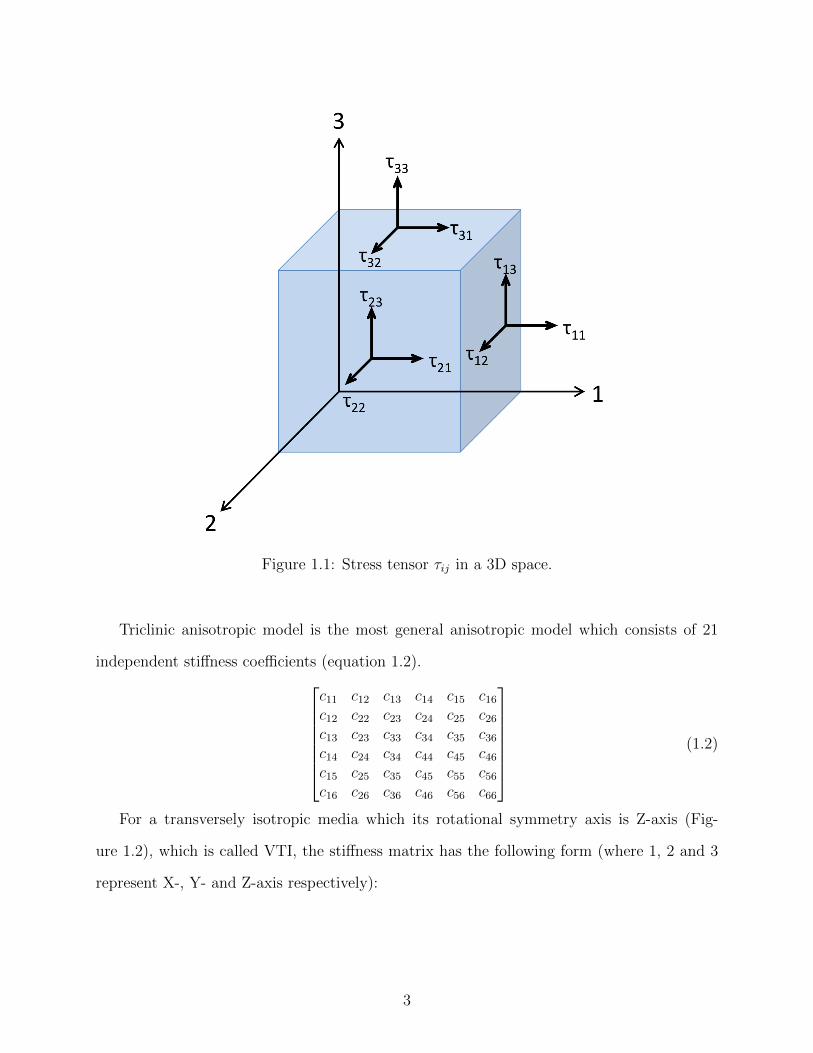
Figure 1.1: Stress tensor τij in a 3D space.

Triclinic anisotropic model is the most general anisotropic model which consists of 21

independent stiffness coefficients (equation 1.2).c11 c12 c13 c14 c15 c16c12 c22 c23 c24 c25 c26c13 c23 c33 c34 c35 c36c14 c24 c34 c44 c45 c46c15 c25 c35 c45 c55 c56c16 c26 c36 c46 c56 c66

(1.2)

For a transversely isotropic media which its rotational symmetry axis is Z-axis (Fig-

ure 1.2), which is called VTI, the stiffness matrix has the following form (where 1, 2 and 3

represent X-, Y- and Z-axis respectively):

3

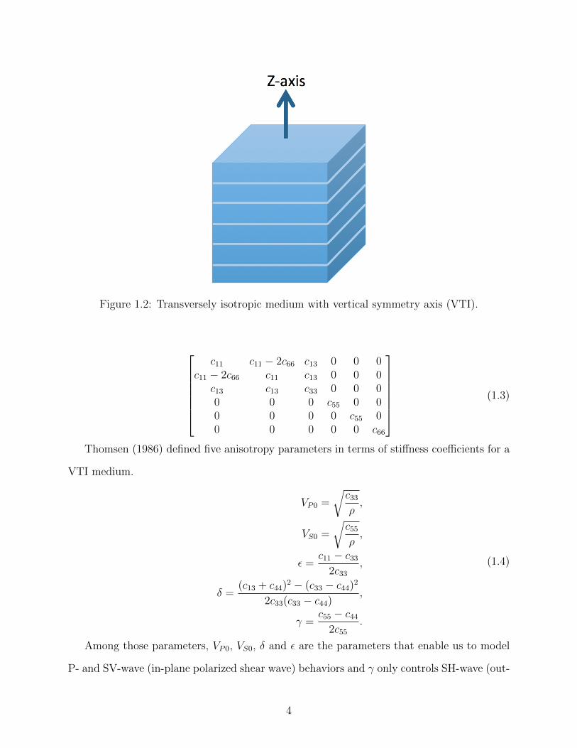
Figure 1.2: Transversely isotropic medium with vertical symmetry axis (VTI).

c11 c11 − 2c66 c13 0 0 0

c11 − 2c66 c11 c13 0 0 0c13 c13 c33 0 0 00 0 0 c55 0 00 0 0 0 c55 00 0 0 0 0 c66

(1.3)

Thomsen (1986) defined five anisotropy parameters in terms of stiffness coefficients for a

VTI medium.

VP0 =

√c33ρ,

VS0 =

√c55ρ,

ε =c11 − c33

2c33,

δ =(c13 + c44)

2 − (c33 − c44)2

2c33(c33 − c44),

γ =c55 − c44

2c55.

(1.4)

Among those parameters, VP0, VS0, δ and ε are the parameters that enable us to model

P- and SV-wave (in-plane polarized shear wave) behaviors and γ only controls SH-wave (out-

4

of-plane polarized shear wave) behaviors. Figure 1.3 shows the effect of δ and ε on P-wave

wavefront (Tsvankin, 2001).

Figure 1.3: P-wave wavefront (solid white) in a VTI medium with ε ≈0.1 and δ ≈-0.1. Theisotropic wavefront with the velocity VP0 is marked by the dashed white line (Tsvankin,2001).

The relationship between above mentioned anisotropy parameters (as well as stiffness

coefficients) and P- and SV-wave velocities and polarizations is explained extensively in

Chapter 2.

1.2 Research Objectives and Values

The main research objectives of this thesis are:

• Modify the slowness-polarization algorithm, called the joint slowness-polarization method,

by incorporating S-wave VSP data to better constrain local anisotropy parameters.

• Assessing the benefits of the joint slowness-polarization method over the conventional

P-wave slowness-polarization method.

5

• Validate the results of joint slowness-polarization method with these of NSGA II wave-

form inversion.

• Modify the moveout-based anisotropic spreading correction (MASC) methodology for

VSP geometry for more accurate azimuthal AVO analysis at the reservoir level.

• Improve the VSP image using anisotropic velocity model which is built using the joint

slowness-polarization method.

Also, the ultimate values of this research are:

1. to identify the existence or lack of open fracture networks at the VSP well location.

2. to improve the quality of final VSP image for future horizontal drilling programs in

this area.

1.3 Case Study

Shale plays are distributed across the US, from the Monterey shale in California to the

Marcellus shale in Pennsylvania and from the Eagle Ford shale in south of Texas to the

Bakken in North Dakota (Figure 1.4). Wide distribution of shale plays in the US suggest

inevitable different geological and geophysical features, which urges more detailed study on

each of these shale plays.

The case study for this research is the Niobrara play in northeast Colorado. A study

by US Energy Information Administration (2014) compares oil and gas production from the

Niobrara Formation with other major shale plays in the US in 2013 and 2014 (Figure 1.5).

Balance between oil and gas production from the Niobrara play, makes it a reliable and

interesting unconventional play for investment and development. Although the total oil and

gas production from the Niobrara play is less than some of unconventional resources, new-

well production, especially new-well oil production, unveils the longterm potential of the

Niobrara (Figure 1.6).

6

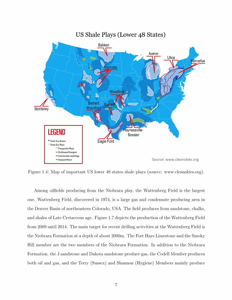
Figure 1.4: Map of important US lower 48 states shale plays (source: www.cleanskies.org).

Among oilfields producing from the Niobrara play, the Wattenberg Field is the largest

one. Wattenberg Field, discovered in 1974, is a large gas and condensate producing area in

the Denver Basin of northeastern Colorado, USA. The field produces from sandstone, chalks,

and shales of Late Cretaceous age. Figure 1.7 depicts the production of the Wattenberg Field

from 2009 until 2014. The main target for recent drilling activities at the Wattenberg Field is

the Niobrara Formation at a depth of about 2000m. The Fort Hays Limestone and the Smoky

Hill member are the two members of the Niobrara Formation. In addition to the Niobrara

Formation, the J sandstone and Dakota sandstone produce gas, the Codell Member produces

both oil and gas, and the Terry (Sussex) and Shannon (Hygiene) Members mainly produce

7

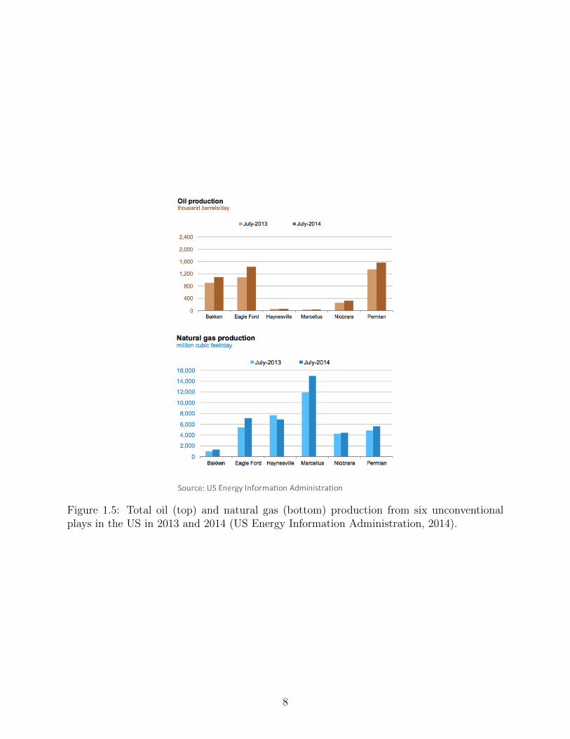
Figure 1.5: Total oil (top) and natural gas (bottom) production from six unconventionalplays in the US in 2013 and 2014 (US Energy Information Administration, 2014).

8

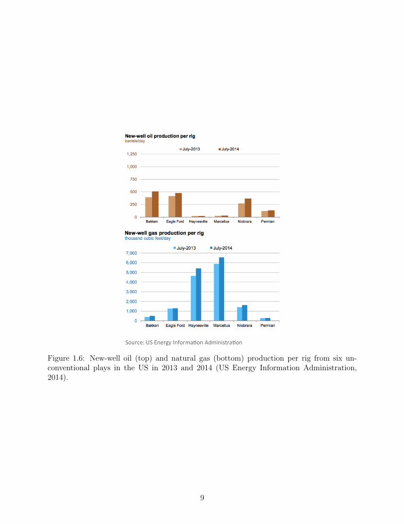
Figure 1.6: New-well oil (top) and natural gas (bottom) production per rig from six un-conventional plays in the US in 2013 and 2014 (US Energy Information Administration,2014).

9

oil at Wattenberg Field (Figure 1.8).

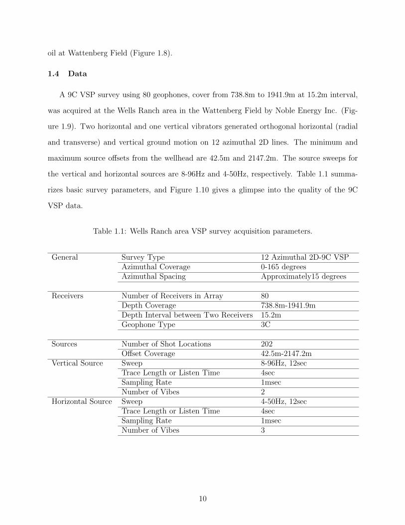
1.4 Data

A 9C VSP survey using 80 geophones, cover from 738.8m to 1941.9m at 15.2m interval,

was acquired at the Wells Ranch area in the Wattenberg Field by Noble Energy Inc. (Fig-

ure 1.9). Two horizontal and one vertical vibrators generated orthogonal horizontal (radial

and transverse) and vertical ground motion on 12 azimuthal 2D lines. The minimum and

maximum source offsets from the wellhead are 42.5m and 2147.2m. The source sweeps for

the vertical and horizontal sources are 8-96Hz and 4-50Hz, respectively. Table 1.1 summa-

rizes basic survey parameters, and Figure 1.10 gives a glimpse into the quality of the 9C

VSP data.

Table 1.1: Wells Ranch area VSP survey acquisition parameters.

General Survey Type 12 Azimuthal 2D-9C VSPAzimuthal Coverage 0-165 degreesAzimuthal Spacing Approximately15 degrees

Receivers Number of Receivers in Array 80Depth Coverage 738.8m-1941.9mDepth Interval between Two Receivers 15.2mGeophone Type 3C

Sources Number of Shot Locations 202Offset Coverage 42.5m-2147.2m

Vertical Source Sweep 8-96Hz, 12secTrace Length or Listen Time 4secSampling Rate 1msecNumber of Vibes 2

Horizontal Source Sweep 4-50Hz, 12secTrace Length or Listen Time 4secSampling Rate 1msecNumber of Vibes 3

10

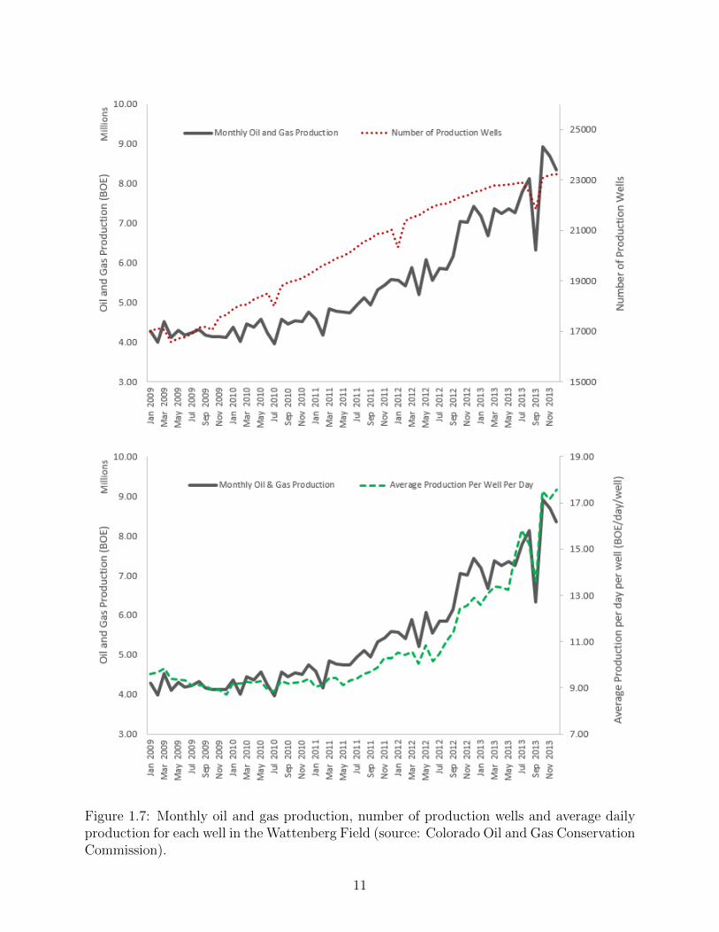
Figure 1.7: Monthly oil and gas production, number of production wells and average dailyproduction for each well in the Wattenberg Field (source: Colorado Oil and Gas ConservationCommission).

11

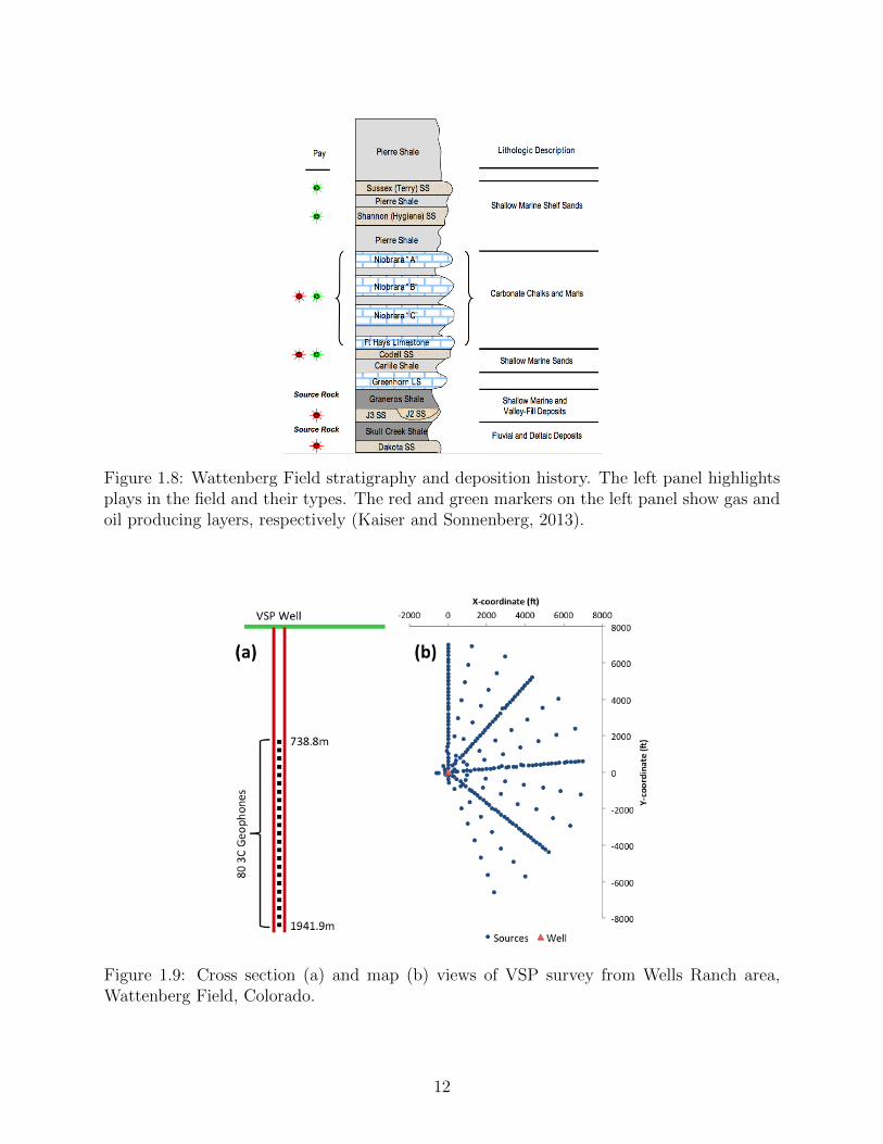
Figure 1.8: Wattenberg Field stratigraphy and deposition history. The left panel highlightsplays in the field and their types. The red and green markers on the left panel show gas andoil producing layers, respectively (Kaiser and Sonnenberg, 2013).

Figure 1.9: Cross section (a) and map (b) views of VSP survey from Wells Ranch area,Wattenberg Field, Colorado.

12

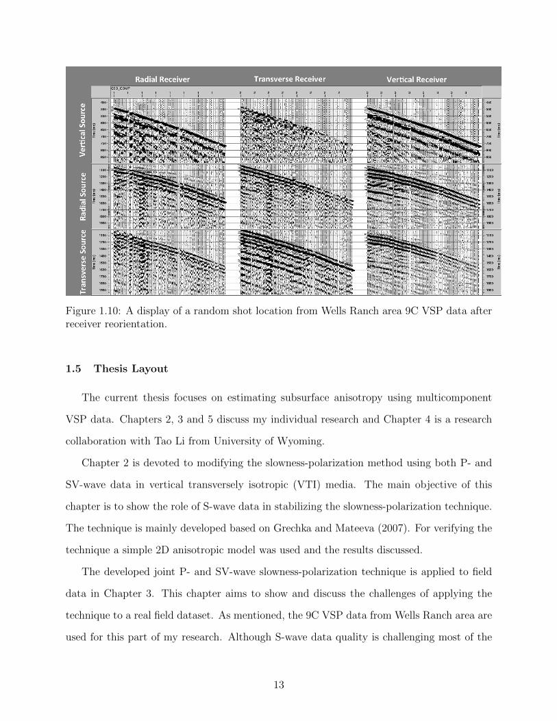
Figure 1.10: A display of a random shot location from Wells Ranch area 9C VSP data afterreceiver reorientation.

1.5 Thesis Layout

The current thesis focuses on estimating subsurface anisotropy using multicomponent

VSP data. Chapters 2, 3 and 5 discuss my individual research and Chapter 4 is a research

collaboration with Tao Li from University of Wyoming.

Chapter 2 is devoted to modifying the slowness-polarization method using both P- and

SV-wave data in vertical transversely isotropic (VTI) media. The main objective of this

chapter is to show the role of S-wave data in stabilizing the slowness-polarization technique.

The technique is mainly developed based on Grechka and Mateeva (2007). For verifying the

technique a simple 2D anisotropic model was used and the results discussed.

The developed joint P- and SV-wave slowness-polarization technique is applied to field

data in Chapter 3. This chapter aims to show and discuss the challenges of applying the

technique to a real field dataset. As mentioned, the 9C VSP data from Wells Ranch area are

used for this part of my research. Although S-wave data quality is challenging most of the

13

times, analyzing final results shows the advantage of the joint inversion approach compared

to a P-wave only approach.

To validate my results from Chapter 3, I need to compare them with results from a

different approach. Chapter 4 presents an alternative approach for estimating anisotropy

parameters from multicomponent VSP data besides the joint slowness-polarization method.

Using waveform inversion, orthorhombic anisotropy parameters are estimated for the Wells

Ranch VSP data. The waveform inversion in this chapter takes advantage of a robust

algorithm, called parallel nondomianted sorting genetic algorithm (NSGA II), to enhance the

performance of the inversion process. The results of the waveform inversion are compared

to the joint P- and S-wave slowness-polarization method.

To show the value of the derived anisotropy model from the previous chapters, Chapter

5 introduces the estimated parameters from the joint slowness-polarization method for an-

alyzing the AVO response and building the final VSP image. To achieve its goal, the first

part of this chapter discusses development of the geometrical spreading correction method

for VSP data based on moveout-based anisotropic spreading correction (MASC) which is

originally developed for surface seismic data (Xu and Tsvankin, 2006; Xu et al., 2005). The

methodology presented in this chapter requires a velocity model for the overburden layers.

The anisotropic velocity model from Chapter 3, which is calibrated in Chapter 4, is the used

anisotropic velocity model for performing the modified MASC technique on VSP data. In

the last part of this chapter, the AVO response and the final VSP image at the reservoir is

discussed and the value of the presented methods in the current thesis is highlighted.

Finally, in Chapter 6, the main conclusions and contributions from this research are

summarized and recommendations for future work are made.

14

CHAPTER 2

USING P- AND S-WAVE VSP DATA FOR ESTIMATING LOCAL SEISMIC

ANISOTROPY PARAMETERS.

Ignoring anisotropy, due to lack of information or work flow complexity, is one of the main

reasons for some challenges in seismic data processing and interpretation. P-wave seismic

data provide valuable information for estimating seismic anisotropy. In addition, acquiring

S-wave seismic data can add significant information to the existing results from P-wave data.

The objective of this research is to introduce a reliable and robust technique for estimating

local seismic anisotropy using both P- and S-wave from VSP data regardless of overburden

complexity. The proposed technique uses P- and SV-wave vertical slowness component

and polarization angle in VTI media to estimate Thomsen parameter δ and anellipticity

parameter η. The proposed technique was applied to a synthetic VSP data and anisotropy

parameters were estimated. The joint P- and SV-wave method could constrain anisotropy

parameters, δ and η, better compared to techniques that only use P-wave data.

2.1 Introduction

A priori information about seismic anisotropy is essential for seismic processing, imaging,

interpretation and reservoir characterization. Ignoring seismic anisotropy causes serious

distortions such as blurry migrated images, misplaced reflectors, incorrect amplitude response

and etc. (Tsvankin and Grechka, 2011). One of the main issues for taking seismic anisotropy

into account is challenges associated with anisotropy parameter estimation.

VSP data are powerful tools to resolve local (also called in-situ) anisotropy with spatial

resolution close to the dominant seismic wavelength (Tsvankin, 2001). Several studies (e.g.

Dewangan and Grechka, 2003; Grechka and Mateeva, 2007; Grechka et al., 2007; Horne and

Leaney, 2000; Miller and Spencer, 1994; Pevzner et al., 2011; Rusmanugroho and McMechan,

2012a,b) have been conducted to estimate local anisotropy using VSP data. The majority

15

of these studies use transmitted (or direct) wave information (i.e. slowness and polarization

vectors) for estimating anisotropy. Because horizontal slowness components are not preserved

in the case of laterally heterogeneous overburden, this information is practically useless in

many studies. In the absence of horizontal slowness components, polarization vector provides

additional information which makes the inversion process more stable but nonlinear.

2.2 Theory of Local Anisotropy Estimation Using VSP Data

A fundamental equation which explains wave propagation in an anisotropic medium using

harmonic plane waves is the Christoffel equation.

[Gik − ρV 2δik]Uk = 0, (2.1)

where ρ is density, V is phase velocity, δik is Kronecker delta, U is polarization vector, and

the Christoffel matrix (Gik) is

Gik = cijklnjnl, (2.2)

where n is the wave propagation direction, and cijkl is the stiffness coefficient. The

eigenvalues of equation (2.1) are found from

det[Gik − ρV 2δik] = 0. (2.3)

Solving equation (2.3) results in three eigenvalues corresponding to three phase velocities,

VP , VS1, and VS2. Substituting each phase velocity into equation (2.1) gives the corresponding

eigenvector or polarization vector U. In anisotropic media, the polarization vector (U) for

each wave mode, except for specific orientations, is different from wave propagation direction

(n). Also, slowness vector (p) for each wave is defined as n/V .

VSP geometry provides a unique opportunity to measure polarization vectors as well as

slowness vectors. Due to these measurements, there are, at least, three different inversion

schemes using VSP data in the literature:

1. Slowness method.

2. Polarization method (MacBeth, 1991).

16

3. Slowness-polarization method.

Among the above mentioned methods, the slowness and the slowness-polarization meth-

ods are more popular. The next two sections explain both methods briefly.

2.2.1 Slowness Method

Estimating local anisotropy from VSP data started with using P-wave slowness data in

the 90’s (Gaiser, 1990; Miller and Spencer, 1994; White et al., 1983). Essential information

for this type of inversion is the slowness vector, p. This information can be derived from

common-receiver gathers, for the horizontal slownesses p1 and p2, and common-shot gathers,

for the vertical slowness p3 or q (Gaiser, 1990).

pi,Q = ∂t/∂xi, (i = 1, 2, 3; Q = P, S1, S2). (2.4)

The slowness inversion technique relies on Snell’s law and the preservation of horizontal

slowness components in laterally homogenous media from the surface to the receiver. But, in

the presence of lateral heterogeneity, this assumption is not valid. Therefore, the horizontal

slownesses cannot be used and the inversion becomes unstable. There are some studies for

correcting the horizontal slowness components in laterally heterogeneous media, but they

are difficult to use practically (Grechka et al., 2006; Jılek et al., 2003).

2.2.2 Slowness-Polarization Method

In the slowness-polarization method, slowness vector p and polarization vector U are

inverted jointly for estimating local anisotropy. The main motivation for development of the

slowness-polarization method is the deficiency associated with the slowness method. Each

source-receiver pair provides one nonlinear equation (2.3) for the stiffness coefficients cijkl.

Therefore, application of the slowness method results in a nonlinear inverse problem whose

solution depends on angular aperture (polar and azimuthal angle) of the VSP data (Tsvankin

and Grechka, 2011). Inversion using all components of P- and S-wave slowness vectors, in

addition to corresponding polarization vectors, is linear. However, the inversion using only

17

P- and S-wave vertical slowness components and polarization vectors is a nonlinear problem.

The second problem is, due to the VSP acquisition geometry, horizontal slowness components

are only measured at the earth’s surface, but we need them at receiver locations. Hence,

lateral homogeneity of the overburden is essential for preserving the horizontal slowness

components and using the slowness method. Unfortunately, lateral homogeneity, especially

within the near surface layers, is not always a valid assumption. In the absence of horizon-

tal slowness components, the polarization vectors provide complementary information for

making the inversion process feasible and more stable.

The above mentioned issues, as well as growth of multicomponent seismic acquisition,

motivated several studies of using slowness and polarization data jointly and resulted in the

slowness-polarization method (de Parscau, 1991; de Parscau and Nicoletis, 1990; Dewan-

gan and Grechka, 2003; Grechka and Mateeva, 2007; Horne and Leaney, 2000; Hsu et al.,

1991; Rusmanugroho and McMechan, 2012a,b). To avoid using horizontal slowness compo-

nents different studies were done using vertical slowness component and polarization vector

(de Parscau, 1991; Dewangan and Grechka, 2003; Hsu et al., 1991; White et al., 1983).

Theoretically, this method is applicable to a subsurface of any complexity (Grechka et al.,

2007).

Dewangan and Grechka (2003) tried to invert vertical slowness and polarization vector

of P-, S1- and S2-waves to obtain the full stiffness tensor of a triclinic medium without

any a priori symmetry assumptions. Dewangan and Grechka (2003) showed that the inver-

sion becomes unstable and introduces considerable errors in the final inversion results when

horizontal slowness components are unknown because of lateral heterogeneity.

Based on studies from de Parscau (1991) and Hsu et al. (1991), joint inversion of vertical

slowness components and polarization vectors of P- and SV-waves can constrain VP0, VS0, ε,

and δ for a VTI medium. These are Thomsen parameters for VTI media (Thomsen, 1986)

18

which are defined as:

VP0 =

√c33ρ,

VS0 =

√c44ρ,

ε =c11 − c33

2c33,

δ =(c13 + c44)

2 − (c33 − c44)2

2c33(c33 − c44).

(2.5)

VP0 and VS0 are vertical P- and S-wave velocities. Grechka and Mateeva (2007) identified

a combination of δ (Thomsen, 1986) and η (Alkhalifah and Tsvankin, 1995) (η = ε−δ1+2δ

)

parameters for VTI and orthorhombic media (Tsvankin, 1997, 2001) which provides an

alternative inversion method for estimating in situ anisotropy using P-wave VSP data. The

identified parameters for VTI media are δV SP and ηV SP , where

δV SP = (f0 − 1)δ, (2.6)

ηV SP = (2f0 − 1)η, (2.7)

f0 =1

1− V 2S0/V

2P0

. (2.8)

In addition, the polarization vector U can be expressed using polar and azimuthal angles:

U = [sinψ cosφ, sinψ sinφ, cosψ], (2.9)

where ψ and φ are polar and azimuthal P-wave polarization angles, respectively. Here,

since the medium is VTI, the polar polarization angle is called just the polarization angle.

By applying perturbation theory (Backus, 1965; Farra, 2001; Psencık and Gajewski, 1998)

in the weak-anisotropy approximation (WAA), P-wave vertical slowness component qP (ψ)

(where qP = p3,P ) for a VTI medium could be expressed in the following form (Grechka and

Mateeva, 2007):

qP (ψ) ≈ cosψ

VP0

[1 + (f0 − 1)δ sin2 ψ + (2f0 − 1)η sin4 ψ]

=cosψ

VP0

[1 + δV SP sin2 ψ + ηV SP sin4 ψ],

(2.10)

19

Equation 2.10 shows that both parameters, δV SP and ηV SP , can be constrained by using

P-wave data and no information from S-wave data is needed. To convert δV SP and ηV SP

parameters to δ and η, the only information which is needed from S-wave data is VS0 (equa-

tions 2.6-2.8). But SV-waves, in addition to providing VS0, might help us constrain the δ and

η parameters. To find out if the SV-wave data add more value to this slowness-polarization

methodology and to get insight into parameters that control the SV-wave vertical slowness

in terms of polarization angle, the weak-anisotropy approximation for SV-wave is derived (I.

Tsvankin, personal communication, 29 September 2014) (See Appendix A for details)

qSV (ψSV ) =sinψSVVS0

[1 + (f0δ − σ) cos2 ψSV + (σ + 2f0η) cos4 ψSV ] (2.11)

=sinψSVVS0

[1 + f0(ε− σ) cos2 ψSV + f0(σ + η) cos4 ψSV ]. (2.12)

where ψSV is the angle between the SV-wave polarization vector and the vertical axis

and σ is the following combination of Thomsen parameters δ and ε (Tsvankin, 2001):

σ ≡(VP0

VS0

)2

(ε− δ). (2.13)

Figure 2.1 compares the exact vertical slowness of SV-wave with the weak-anisotropy

approximation.

According to equation 2.11, the qSV (ψSV ) is controlled by σ, ε and η. In weak anisotropic

media, we have

η ≈ (ε− δ),

σ ≈(VP0

VS0

)2

η.(2.14)

From equations 2.11 and 2.14, estimation of η should be improved when SV-wave data

are used for the inversion. To explain why and at what polarization the function qSV (ψSV )

can constrain δ, a different form of the equation is derived for the weak anisotropic media

(V. Grechka, personal communication, 20 October 2014):


[1 + f0 cos2 ψSV (δ +(2f0 − 1) cos2 ψSV − 1

f0 − 1η)]. (2.15)

20

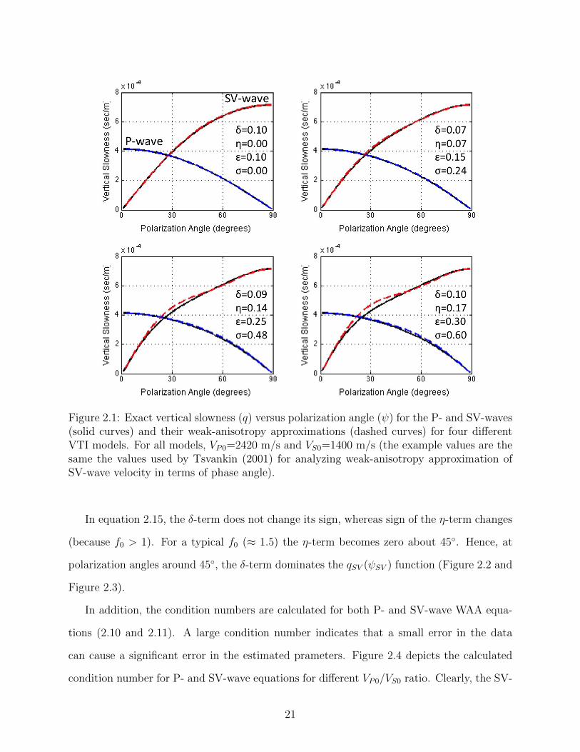
Figure 2.1: Exact vertical slowness (q) versus polarization angle (ψ) for the P- and SV-waves(solid curves) and their weak-anisotropy approximations (dashed curves) for four differentVTI models. For all models, VP0=2420 m/s and VS0=1400 m/s (the example values are thesame the values used by Tsvankin (2001) for analyzing weak-anisotropy approximation ofSV-wave velocity in terms of phase angle).

In equation 2.15, the δ-term does not change its sign, whereas sign of the η-term changes

(because f0 > 1). For a typical f0 (≈ 1.5) the η-term becomes zero about 45◦. Hence, at

polarization angles around 45◦, the δ-term dominates the qSV (ψSV ) function (Figure 2.2 and

Figure 2.3).

In addition, the condition numbers are calculated for both P- and SV-wave WAA equa-

tions (2.10 and 2.11). A large condition number indicates that a small error in the data

can cause a significant error in the estimated prameters. Figure 2.4 depicts the calculated

condition number for P- and SV-wave equations for different VP0/VS0 ratio. Clearly, the SV-

21

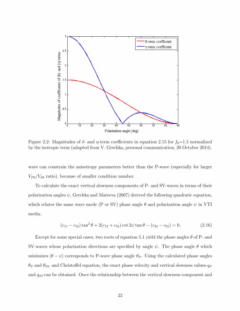
Figure 2.2: Magnitudes of δ- and η-term coefficients in equation 2.15 for f0=1.5 normalizedby the isotropic term (adapted from V. Grechka, personal communication, 20 October 2014).

wave can constrain the anisotropy parameters better than the P-wave (especially for larger

VP0/VS0 ratio), because of smaller condition number.

To calculate the exact vertical slowness components of P- and SV-waves in terms of their

polarization angles ψ, Grechka and Mateeva (2007) derived the following quadratic equation,

which relates the same wave mode (P or SV) phase angle θ and polarization angle ψ in VTI

media.

(c11 − c55) tan2 θ + 2(c13 + c55) cot 2ψ tan θ − (c33 − c55) = 0. (2.16)

Except for some special cases, two roots of equation 5.1 yield the phase angles θ of P- and

SV-waves whose polarization directions are specified by angle ψ. The phase angle θ which

minimizes |θ − ψ| corresponds to P-wave phase angle θP . Using the calculated phase angles

θP and θSV and Christoffel equation, the exact phase velocity and vertical slowness values qP

and qSV can be obtained. Once the relationship between the vertical slowness component and

22

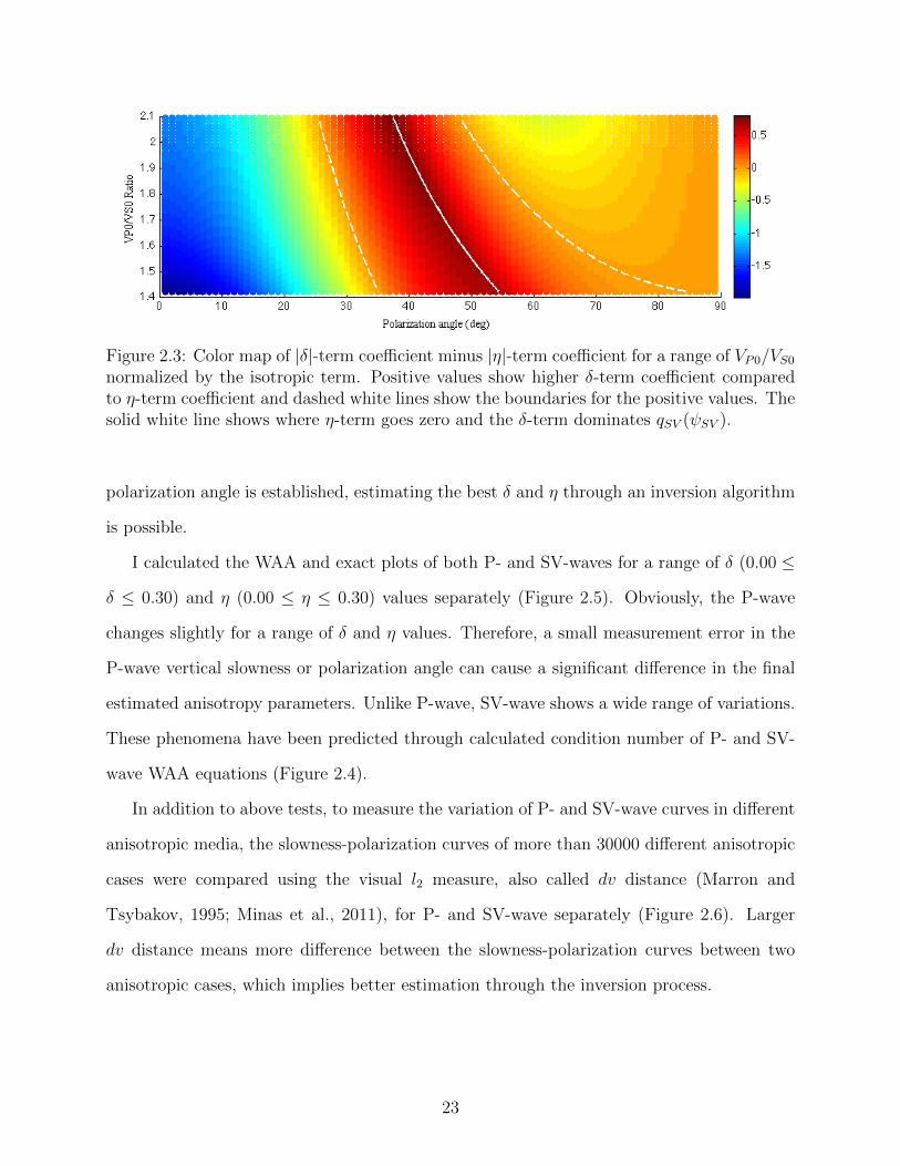
Figure 2.3: Color map of |δ|-term coefficient minus |η|-term coefficient for a range of VP0/VS0normalized by the isotropic term. Positive values show higher δ-term coefficient comparedto η-term coefficient and dashed white lines show the boundaries for the positive values. Thesolid white line shows where η-term goes zero and the δ-term dominates qSV (ψSV ).

polarization angle is established, estimating the best δ and η through an inversion algorithm

is possible.

I calculated the WAA and exact plots of both P- and SV-waves for a range of δ (0.00 ≤

δ ≤ 0.30) and η (0.00 ≤ η ≤ 0.30) values separately (Figure 2.5). Obviously, the P-wave

changes slightly for a range of δ and η values. Therefore, a small measurement error in the

P-wave vertical slowness or polarization angle can cause a significant difference in the final

estimated anisotropy parameters. Unlike P-wave, SV-wave shows a wide range of variations.

These phenomena have been predicted through calculated condition number of P- and SV-

wave WAA equations (Figure 2.4).

In addition to above tests, to measure the variation of P- and SV-wave curves in different

anisotropic media, the slowness-polarization curves of more than 30000 different anisotropic

cases were compared using the visual l2 measure, also called dv distance (Marron and

Tsybakov, 1995; Minas et al., 2011), for P- and SV-wave separately (Figure 2.6). Larger

dv distance means more difference between the slowness-polarization curves between two

anisotropic cases, which implies better estimation through the inversion process.

23

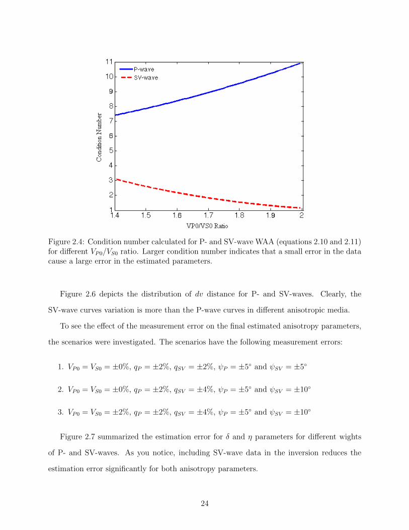
Figure 2.4: Condition number calculated for P- and SV-wave WAA (equations 2.10 and 2.11)for different VP0/VS0 ratio. Larger condition number indicates that a small error in the datacause a large error in the estimated parameters.

Figure 2.6 depicts the distribution of dv distance for P- and SV-waves. Clearly, the

SV-wave curves variation is more than the P-wave curves in different anisotropic media.

To see the effect of the measurement error on the final estimated anisotropy parameters,

the scenarios were investigated. The scenarios have the following measurement errors:

1. VP0 = VS0 = ±0%, qP = ±2%, qSV = ±2%, ψP = ±5◦ and ψSV = ±5◦



Figure 2.7 summarized the estimation error for δ and η parameters for different wights

of P- and SV-waves. As you notice, including SV-wave data in the inversion reduces the

estimation error significantly for both anisotropy parameters.

24

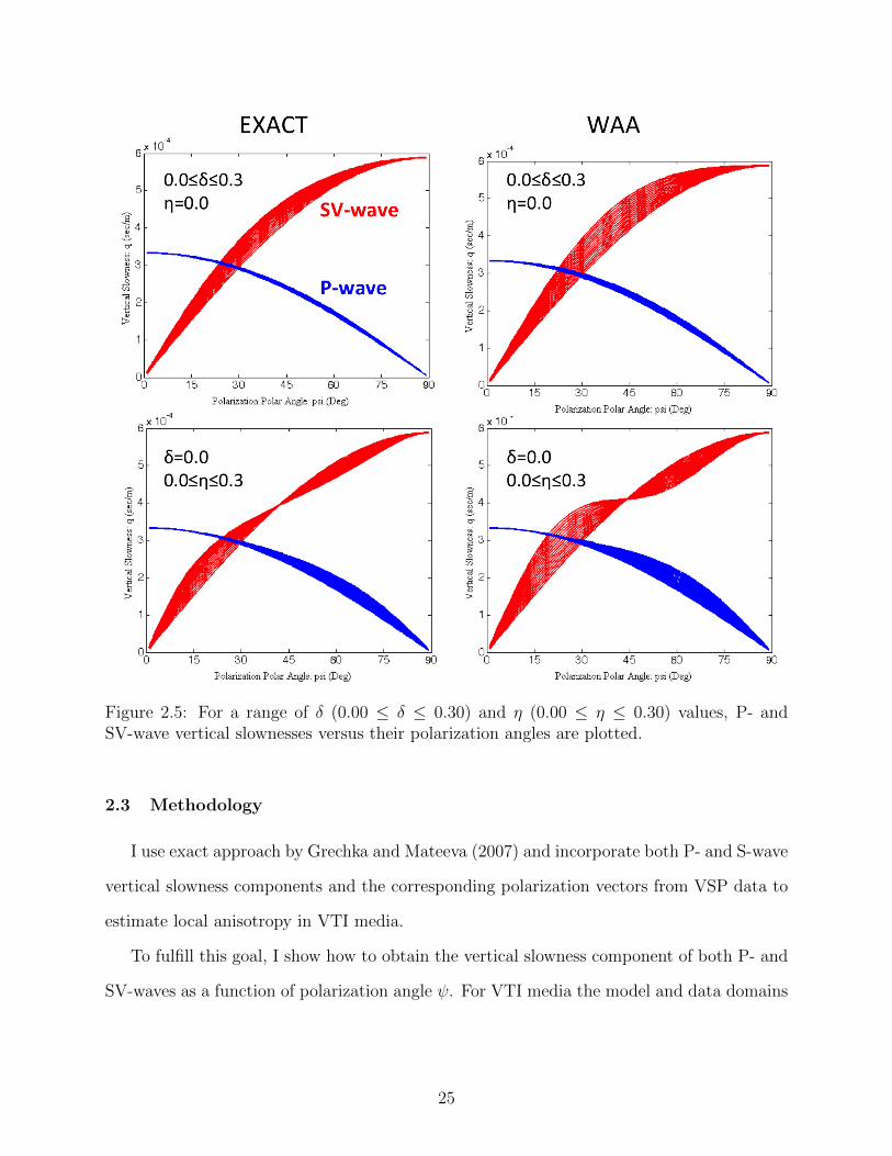
Figure 2.5: For a range of δ (0.00 ≤ δ ≤ 0.30) and η (0.00 ≤ η ≤ 0.30) values, P- andSV-wave vertical slownesses versus their polarization angles are plotted.

2.3 Methodology

I use exact approach by Grechka and Mateeva (2007) and incorporate both P- and S-wave

vertical slowness components and the corresponding polarization vectors from VSP data to

estimate local anisotropy in VTI media.

To fulfill this goal, I show how to obtain the vertical slowness component of both P- and

SV-waves as a function of polarization angle ψ. For VTI media the model and data domains

25

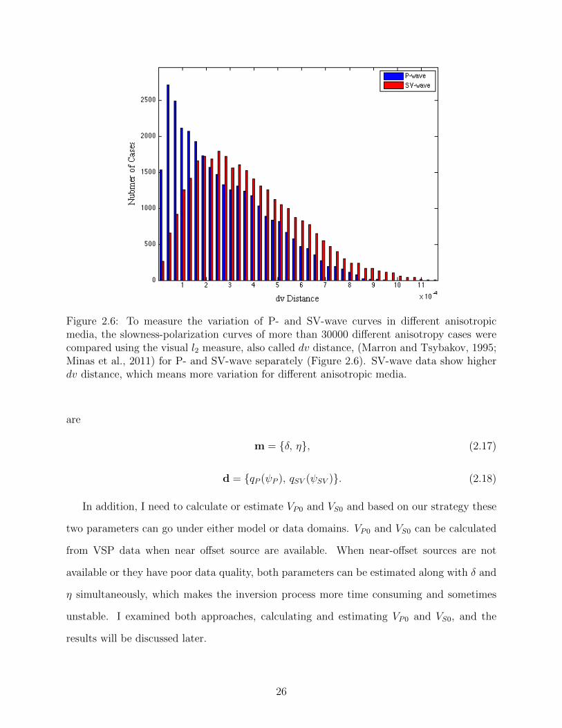
Figure 2.6: To measure the variation of P- and SV-wave curves in different anisotropicmedia, the slowness-polarization curves of more than 30000 different anisotropy cases werecompared using the visual l2 measure, also called dv distance, (Marron and Tsybakov, 1995;Minas et al., 2011) for P- and SV-wave separately (Figure 2.6). SV-wave data show higherdv distance, which means more variation for different anisotropic media.

are

m = {δ, η}, (2.17)

d = {qP (ψP ), qSV (ψSV )}. (2.18)

In addition, I need to calculate or estimate VP0 and VS0 and based on our strategy these

two parameters can go under either model or data domains. VP0 and VS0 can be calculated

from VSP data when near offset source are available. When near-offset sources are not

available or they have poor data quality, both parameters can be estimated along with δ and

η simultaneously, which makes the inversion process more time consuming and sometimes

unstable. I examined both approaches, calculating and estimating VP0 and VS0, and the

results will be discussed later.

26

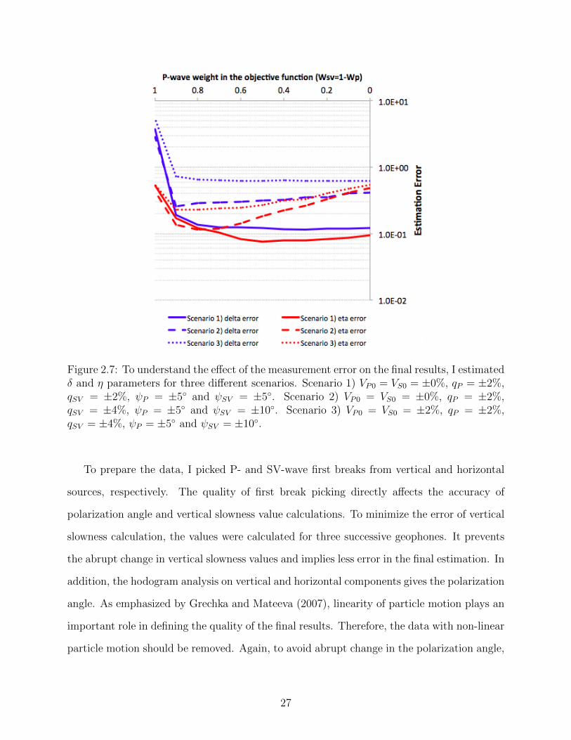
Figure 2.7: To understand the effect of the measurement error on the final results, I estimatedδ and η parameters for three different scenarios. Scenario 1) VP0 = VS0 = ±0%, qP = ±2%,qSV = ±2%, ψP = ±5◦ and ψSV = ±5◦. Scenario 2) VP0 = VS0 = ±0%, qP = ±2%,qSV = ±4%, ψP = ±5◦ and ψSV = ±10◦. Scenario 3) VP0 = VS0 = ±2%, qP = ±2%,qSV = ±4%, ψP = ±5◦ and ψSV = ±10◦.

To prepare the data, I picked P- and SV-wave first breaks from vertical and horizontal

sources, respectively. The quality of first break picking directly affects the accuracy of

polarization angle and vertical slowness value calculations. To minimize the error of vertical

slowness calculation, the values were calculated for three successive geophones. It prevents

the abrupt change in vertical slowness values and implies less error in the final estimation. In

addition, the hodogram analysis on vertical and horizontal components gives the polarization

angle. As emphasized by Grechka and Mateeva (2007), linearity of particle motion plays an

important role in defining the quality of the final results. Therefore, the data with non-linear

particle motion should be removed. Again, to avoid abrupt change in the polarization angle,

27

I took the average of the polarization angle of every three geophones.

Finally, the following objective function is defined and minimized with respect to m.

E(m) = WPΣ[qcalcP (m, ψP )− qP (ψP )]2 +WSV Σ[qcalcSV (m, ψSV )− qSV (ψSV )]2, (2.19)

where WP and WSV are weights of the P- and SV-wave contributions. WP and WSV can

be adjusted based on the desired scenario and the data quality. When P-wave data is used

only, WP = 1.0 and WSV = 0.0, and in the joint optimization case, WP = 0.5 and WSV = 0.5.

Also, based on the error in calculating P- and SV-wave vertical slowness components and

polarization angles, WP and WSV can be adjusted.

2.4 9C Synthetic VSP Data

To verify the proposed technique and compare it with other techniques, a simple 2D

anisotropic model is built, and 9C VSP data using 26 geophones were generated (Figure 2.8).

The model is composed of four horizontal layers, three of them are VTI and the shallowest

layer is isotropic. The geophones covered the 1400 m to 2900 m depth interval and at 60m

interval. The data were acquired at 61 shot locations, using vertical and horizontal sources,

at 150 m interval with minimum and maximum offset of 100 m and 6100 m from the wellhead,

respectively. The recorded traces are 5000 ms and the wavelet has frequencies up to 55 Hz.

The multicomponent VSP data were generated using the finite-difference modeling algo-

rithm. Figure 2.9 displays a snapshot of the data quality and the P- and SV-wave first-break

arrivals. As the source offset increases, the first break picking quality decreases. To en-

hance the quality of first-break picking, especially for far offset shots, the geophones were

mathematically rotated in such a way to maximize P- or SV-waves energy on one of the

components for both vertical and horizontal sources.

In addition to first break arrivals, the error in polarization angle calculation can signifi-

cantly change the final results. A cause for polarization angle calculation error is nonlinear

particle motion. More linear particle motion in hodogram analysis leads to better calcula-

28

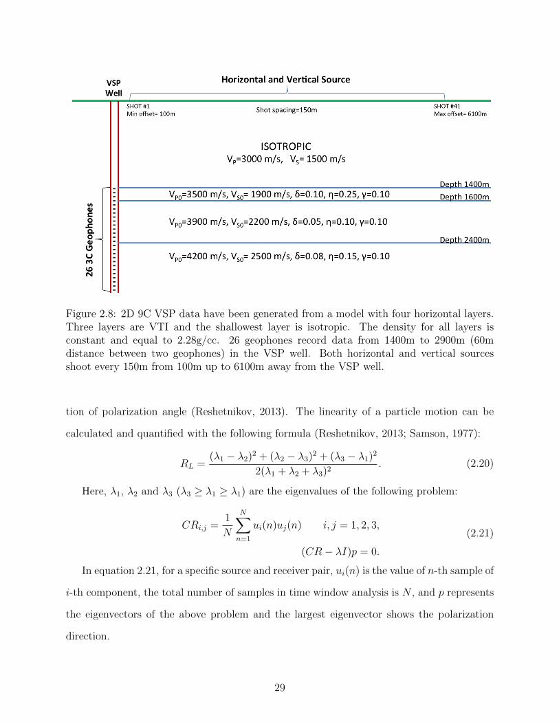
Figure 2.8: 2D 9C VSP data have been generated from a model with four horizontal layers.Three layers are VTI and the shallowest layer is isotropic. The density for all layers isconstant and equal to 2.28g/cc. 26 geophones record data from 1400m to 2900m (60mdistance between two geophones) in the VSP well. Both horizontal and vertical sourcesshoot every 150m from 100m up to 6100m away from the VSP well.

tion of polarization angle (Reshetnikov, 2013). The linearity of a particle motion can be

calculated and quantified with the following formula (Reshetnikov, 2013; Samson, 1977):

RL =(λ1 − λ2)2 + (λ2 − λ3)2 + (λ3 − λ1)2

2(λ1 + λ2 + λ3)2. (2.20)

Here, λ1, λ2 and λ3 (λ3 ≥ λ1 ≥ λ1) are the eigenvalues of the following problem:

CRi,j =1

N

N∑n=1

ui(n)uj(n) i, j = 1, 2, 3,

(CR− λI)p = 0.

(2.21)

In equation 2.21, for a specific source and receiver pair, ui(n) is the value of n-th sample of

i-th component, the total number of samples in time window analysis is N , and p represents

the eigenvectors of the above problem and the largest eigenvector shows the polarization

direction.

29

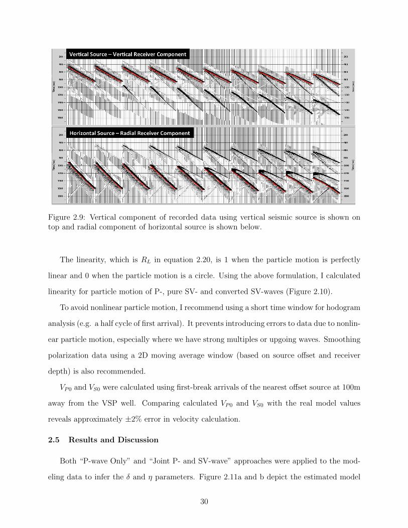
Figure 2.9: Vertical component of recorded data using vertical seismic source is shown ontop and radial component of horizontal source is shown below.

The linearity, which is RL in equation 2.20, is 1 when the particle motion is perfectly

linear and 0 when the particle motion is a circle. Using the above formulation, I calculated

linearity for particle motion of P-, pure SV- and converted SV-waves (Figure 2.10).

To avoid nonlinear particle motion, I recommend using a short time window for hodogram

analysis (e.g. a half cycle of first arrival). It prevents introducing errors to data due to nonlin-

ear particle motion, especially where we have strong multiples or upgoing waves. Smoothing

polarization data using a 2D moving average window (based on source offset and receiver

depth) is also recommended.

VP0 and VS0 were calculated using first-break arrivals of the nearest offset source at 100m

away from the VSP well. Comparing calculated VP0 and VS0 with the real model values

reveals approximately ±2% error in velocity calculation.

2.5 Results and Discussion

Both “P-wave Only” and “Joint P- and SV-wave” approaches were applied to the mod-

eling data to infer the δ and η parameters. Figure 2.11a and b depict the estimated model

30

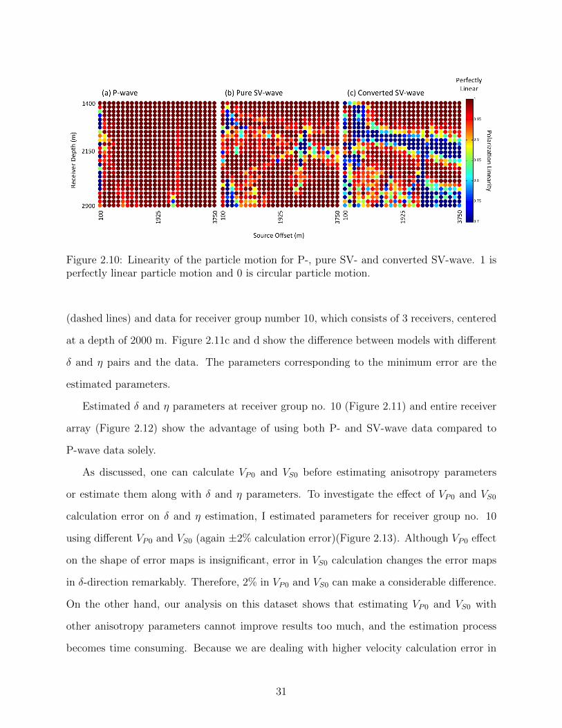
Figure 2.10: Linearity of the particle motion for P-, pure SV- and converted SV-wave. 1 isperfectly linear particle motion and 0 is circular particle motion.

(dashed lines) and data for receiver group number 10, which consists of 3 receivers, centered

at a depth of 2000 m. Figure 2.11c and d show the difference between models with different

δ and η pairs and the data. The parameters corresponding to the minimum error are the

estimated parameters.

Estimated δ and η parameters at receiver group no. 10 (Figure 2.11) and entire receiver

array (Figure 2.12) show the advantage of using both P- and SV-wave data compared to

P-wave data solely.

As discussed, one can calculate VP0 and VS0 before estimating anisotropy parameters

or estimate them along with δ and η parameters. To investigate the effect of VP0 and VS0

calculation error on δ and η estimation, I estimated parameters for receiver group no. 10

using different VP0 and VS0 (again ±2% calculation error)(Figure 2.13). Although VP0 effect

on the shape of error maps is insignificant, error in VS0 calculation changes the error maps

in δ-direction remarkably. Therefore, 2% in VP0 and VS0 can make a considerable difference.

On the other hand, our analysis on this dataset shows that estimating VP0 and VS0 with

other anisotropy parameters cannot improve results too much, and the estimation process

becomes time consuming. Because we are dealing with higher velocity calculation error in

31

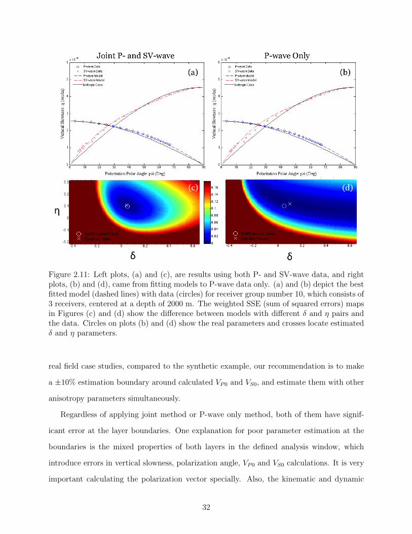
Figure 2.11: Left plots, (a) and (c), are results using both P- and SV-wave data, and rightplots, (b) and (d), came from fitting models to P-wave data only. (a) and (b) depict the bestfitted model (dashed lines) with data (circles) for receiver group number 10, which consists of3 receivers, centered at a depth of 2000 m. The weighted SSE (sum of squared errors) mapsin Figures (c) and (d) show the difference between models with different δ and η pairs andthe data. Circles on plots (b) and (d) show the real parameters and crosses locate estimatedδ and η parameters.

real field case studies, compared to the synthetic example, our recommendation is to make

a ±10% estimation boundary around calculated VP0 and VS0, and estimate them with other

anisotropy parameters simultaneously.

Regardless of applying joint method or P-wave only method, both of them have signif-

icant error at the layer boundaries. One explanation for poor parameter estimation at the

boundaries is the mixed properties of both layers in the defined analysis window, which

introduce errors in vertical slowness, polarization angle, VP0 and VS0 calculations. It is very

important calculating the polarization vector specially. Also, the kinematic and dynamic

32

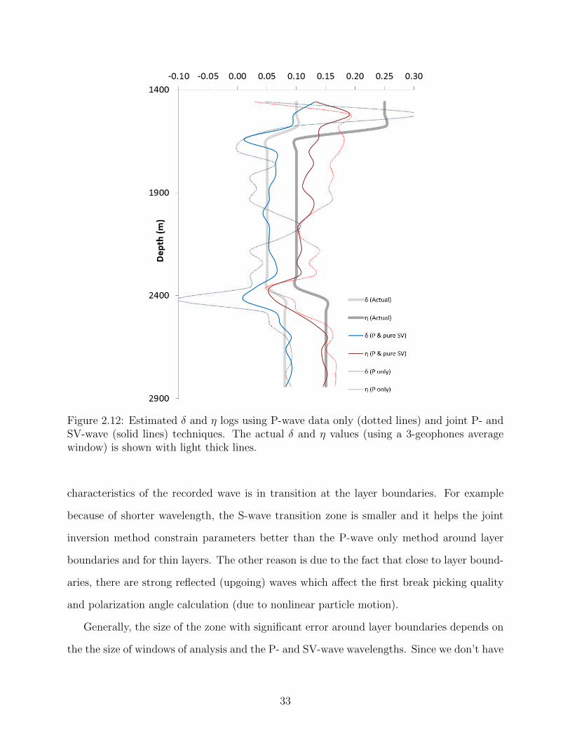
Figure 2.12: Estimated δ and η logs using P-wave data only (dotted lines) and joint P- andSV-wave (solid lines) techniques. The actual δ and η values (using a 3-geophones averagewindow) is shown with light thick lines.

characteristics of the recorded wave is in transition at the layer boundaries. For example

because of shorter wavelength, the S-wave transition zone is smaller and it helps the joint

inversion method constrain parameters better than the P-wave only method around layer

boundaries and for thin layers. The other reason is due to the fact that close to layer bound-

aries, there are strong reflected (upgoing) waves which affect the first break picking quality

and polarization angle calculation (due to nonlinear particle motion).

Generally, the size of the zone with significant error around layer boundaries depends on

the the size of windows of analysis and the P- and SV-wave wavelengths. Since we don’t have

33

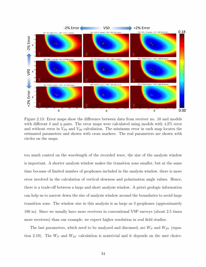
Figure 2.13: Error maps show the difference between data from receiver no. 10 and modelswith different δ and η pairs. The error maps were calculated using models with ±2% errorand without error in VP0 and VS0 calculation. The minimum error in each map locates theestimated parameters and shown with cross markers. The real parameters are shown withcircles on the maps.

too much control on the wavelength of the recorded wave, the size of the analysis window

is important. A shorter analysis window makes the transition zone smaller, but at the same

time because of limited number of geophones included in the analysis window, there is more

error involved in the calculation of vertical slowness and polarization angle values. Hence,

there is a trade-off between a large and short analysis window. A priori geologic information

can help us to narrow down the size of analysis window around the boundaries to avoid large

transition zone. The window size in this analysis is as large as 3 geophones (approximately

180 m). Since we usually have more receivers in conventional VSP surveys (about 2.5 times

more receivers) than our example, we expect higher resolution in real field studies.

The last parameters, which need to be analyzed and discussed, are WP and WSV (equa-

tion 2.19). The WP and WSV calculation is nontrivial and it depends on the user choice.

34

However, as mentioned, factors such as data quality might affect the choice of WP and WSV .

To understand the importance of WP and WSV calculation, the δ and η parameters were

estimated using different P- and SV-wave weight combinations and the results were com-

pared with real δ and η parameters (Figure 2.14 and Figure 2.15). The sensitivity analysis

confirms the advantage of involving both P- and SV-wave data in the inversion process.

Because acquiring pure S-wave (that is generated by horizontal sources) is not common

and many VSP surveys record converted S-wave data using 3C geophones, the same joint

inversion approach was repeated with P- and converted SV-wave data. Figure 2.16 depicts

the results of joint inversion of P- and converted SV-wave data and compare them with the

results of joint P- and pure (or non-converted) SV-wave inversion. Clearly, pure SV-wave

data helped the joint slowness-polarization method constrain anisotropy parameters, δ and

η, better. Figure 2.17 compares the polarization angle of pure SV- and converted SV-wave

data which were used in the joint inversions.

One explanation for better estimation of the inversion using pure SV-wave data compared

to converted SV-wave data is their larger aperture according to Figure 2.17. For the model in

this study, on average, converted SV-wave covers 30◦ less polarization angle range compared

to pure SV-wave. Another explanation for better results of the joint method with pure SV-

wave data is because of the converted SV-wave particle motion. As shown in Figure 2.10,

pure SV-wave data have more linear particle motion than converted SV-wave data, which

cause less error in their polarization angle calculation. The P-wave multiples and reflections

as well as lower signal to noise ratio are two reasons for nonlinear particle motion of converted

SV-wave data.

Figure 2.18 summarizes the error of estimated parameters for all three approaches in

this chapter, which are P-wave data only, joint P- and pure SV-wave data and joint P- and

converted SV-wave data. Without doubt, the joint P- and pure SV-wave inversion could

constrain anisotropy parameters, δ and η better than the two other approaches. Except for

depth below 2400 m, the joint P- and converted SV-wave data provided better estimation

35

compared to P-wave data.

2.6 Conclusions

The SV-wave data were incorporated into the slowness-polarization methodology pro-

posed by Grechka and Mateeva (2007). Assessing SV-wave data quality, having sufficient

source offset coverage, as well as determining a reasonable depth window size for analysis

based on local stratigraphy are important factors which should be considered before the

inversion.

The results showed that using the joint P- and SV-wave slowness-polarization method, δ

and η parameters can be estimated better compared to the methods that use P-wave data

only. Also, because of higher data aperture and more linear particle motion, pure SV-wave

data can help the joint slowness-polarization method constrain anisotropy parameters better

than converted SV-wave data.

Although the joint inversion method gives us better estimation of δ and η parameters,

estimating parameters at layer boundaries and in thin layers is the most important challenge.

36

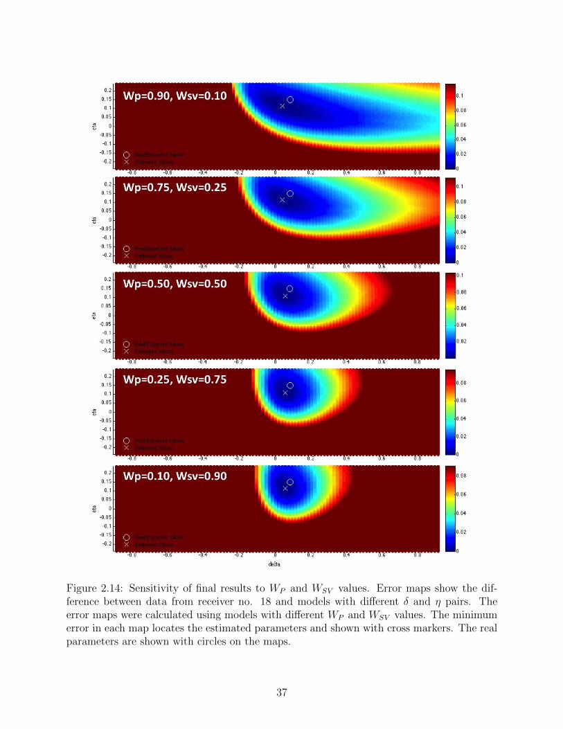
Figure 2.14: Sensitivity of final results to WP and WSV values. Error maps show the dif-ference between data from receiver no. 18 and models with different δ and η pairs. Theerror maps were calculated using models with different WP and WSV values. The minimumerror in each map locates the estimated parameters and shown with cross markers. The realparameters are shown with circles on the maps.

37

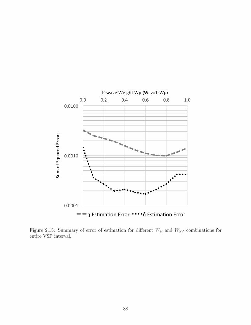
Figure 2.15: Summary of error of estimation for different WP and WSV combinations forentire VSP interval.

38

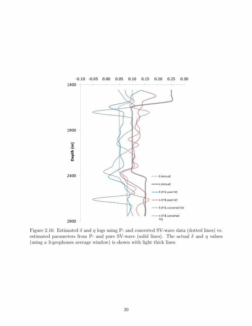
Figure 2.16: Estimated δ and η logs using P- and converted SV-wave data (dotted lines) vs.estimated parameters from P- and pure SV-wave (solid lines). The actual δ and η values(using a 3-geophones average window) is shown with light thick lines.

39

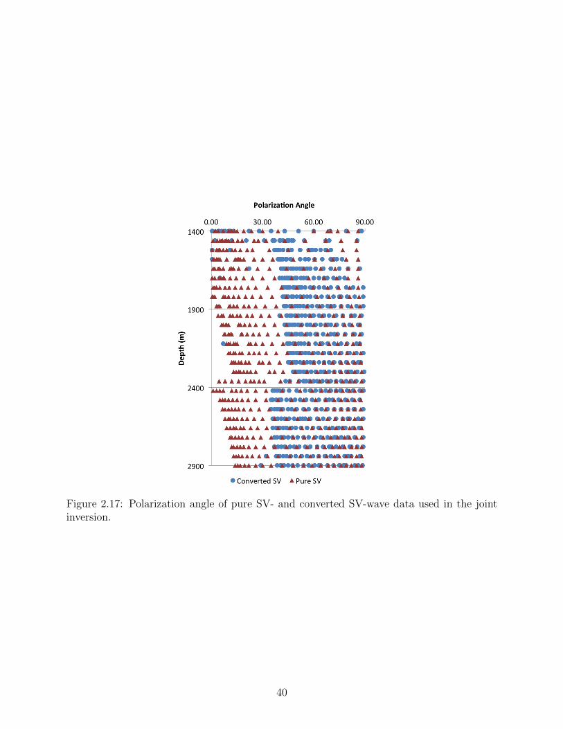
Figure 2.17: Polarization angle of pure SV- and converted SV-wave data used in the jointinversion.

40

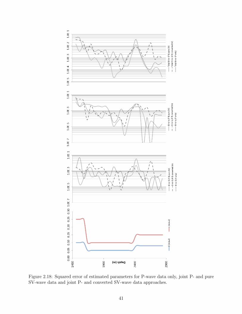
Figure 2.18: Squared error of estimated parameters for P-wave data only, joint P- and pureSV-wave data and joint P- and converted SV-wave data approaches.

41

CHAPTER 3

ESTIMATING LOCAL SEISMIC ANISOTROPY PARAMETERS USING P- AND

SV-WAVE VERTICAL SLOWNESS COMPONENTS AND POLARIZATION ANGLES

AT WELLS RANCH AREA, WATTENBERG FIELD, COLORADO.

Subsurface anisotropy information is important for processing, imaging and interpreta-

tion of surface and borehole seismic data. The slowness-polarization method is one of the

techniques using VSP data to constrain local anisotropy parameters around the receiver ar-

ray in the VSP well. Although the technique can be applied using P-wave data only, using

both P- and S-wave data make the technique more robust and reliable.

The objective of this chapter is to show the application of the joint P- and S-wave

slowness-polarization method in a real field case study. The study VSP well is located at

Wells Ranch area, Wattenberg Field, Colorado. 9C VSP data provide an opportunity to

study different aspects of the technique, and derive important anisotropy information above

the Niobrara Formation at this area.

Due to evidence from VSP data about the presence of orthorhombic anisotropy at some

levels, the slowness-polarization method is applied in two symmetry planes (i.e. SE and NE

directions). The joint P- and SV-wave method led to significant improvement in δ and η

determination.

3.1 Introduction

In the previous chapter, I developed the joint P- and SV-wave slowness-polarization

method and applied the technique to a synthetic VSP dataset. The final results showed that

the anisotropy parameters δ and η can be constrained better using both P- and SV-wave

data. In this chapter, I apply the joint slowness-polarization method to a real field data.

First, the case study for this research is introduced, and then the results are discussed.

42

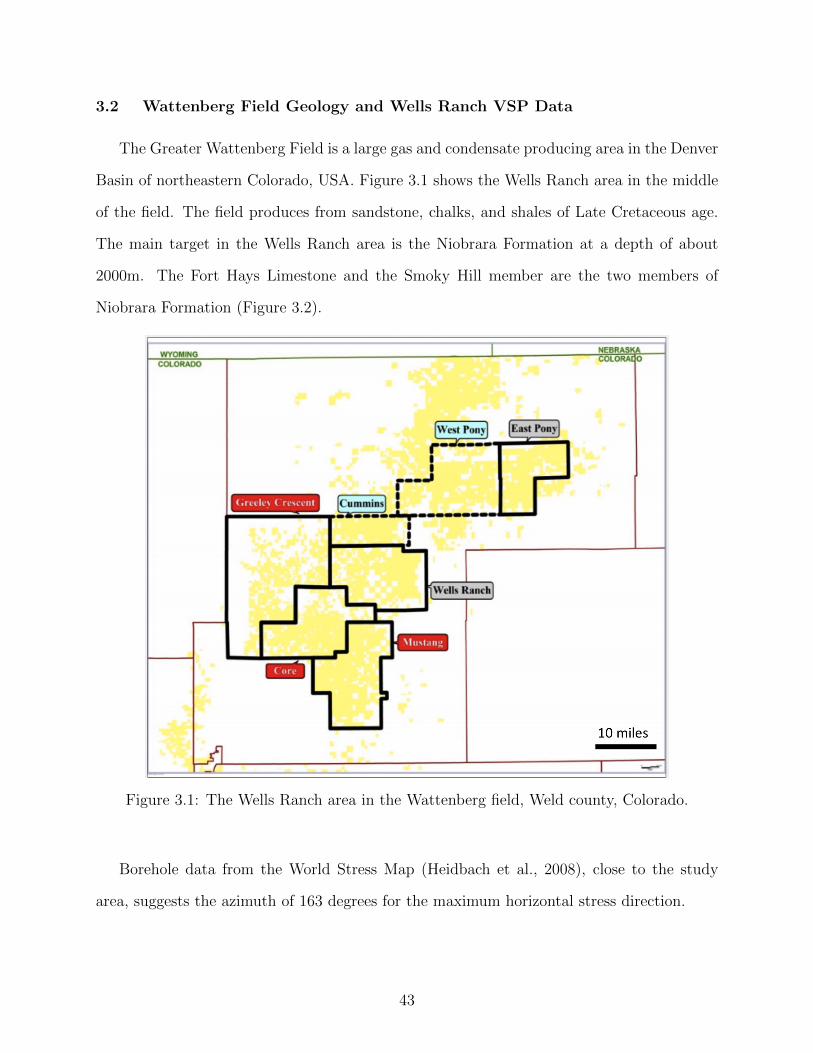
3.2 Wattenberg Field Geology and Wells Ranch VSP Data

The Greater Wattenberg Field is a large gas and condensate producing area in the Denver

Basin of northeastern Colorado, USA. Figure 3.1 shows the Wells Ranch area in the middle

of the field. The field produces from sandstone, chalks, and shales of Late Cretaceous age.

The main target in the Wells Ranch area is the Niobrara Formation at a depth of about

2000m. The Fort Hays Limestone and the Smoky Hill member are the two members of

Niobrara Formation (Figure 3.2).

Figure 3.1: The Wells Ranch area in the Wattenberg field, Weld county, Colorado.

Borehole data from the World Stress Map (Heidbach et al., 2008), close to the study

area, suggests the azimuth of 163 degrees for the maximum horizontal stress direction.

43

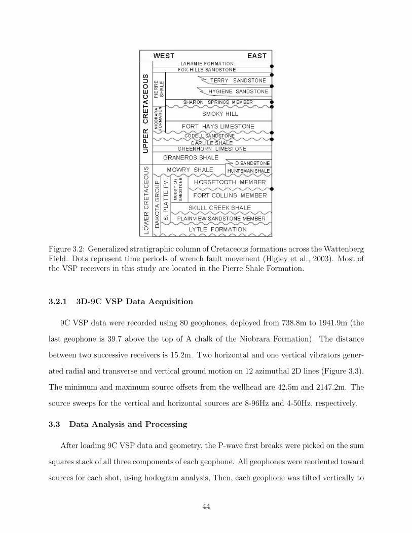
Figure 3.2: Generalized stratigraphic column of Cretaceous formations across the WattenbergField. Dots represent time periods of wrench fault movement (Higley et al., 2003). Most ofthe VSP receivers in this study are located in the Pierre Shale Formation.

3.2.1 3D-9C VSP Data Acquisition

9C VSP data were recorded using 80 geophones, deployed from 738.8m to 1941.9m (the

last geophone is 39.7 above the top of A chalk of the Niobrara Formation). The distance

between two successive receivers is 15.2m. Two horizontal and one vertical vibrators gener-

ated radial and transverse and vertical ground motion on 12 azimuthal 2D lines (Figure 3.3).

The minimum and maximum source offsets from the wellhead are 42.5m and 2147.2m. The

source sweeps for the vertical and horizontal sources are 8-96Hz and 4-50Hz, respectively.

3.3 Data Analysis and Processing

After loading 9C VSP data and geometry, the P-wave first breaks were picked on the sum

squares stack of all three components of each geophone. All geophones were reoriented toward

sources for each shot, using hodogram analysis, Then, each geophone was tilted vertically to

44

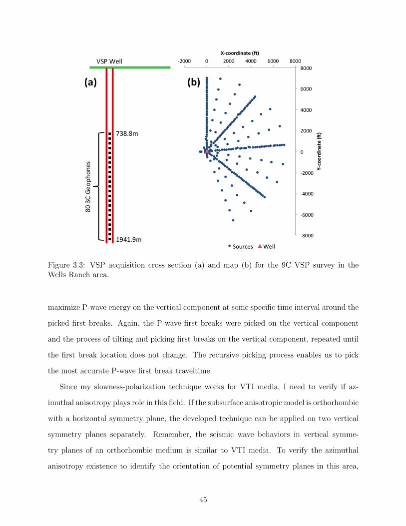
Figure 3.3: VSP acquisition cross section (a) and map (b) for the 9C VSP survey in theWells Ranch area.

maximize P-wave energy on the vertical component at some specific time interval around the

picked first breaks. Again, the P-wave first breaks were picked on the vertical component

and the process of tilting and picking first breaks on the vertical component, repeated until

the first break location does not change. The recursive picking process enables us to pick

the most accurate P-wave first break traveltime.

Since my slowness-polarization technique works for VTI media, I need to verify if az-

imuthal anisotropy plays role in this field. If the subsurface anisotropic model is orthorhombic

with a horizontal symmetry plane, the developed technique can be applied on two vertical

symmetry planes separately. Remember, the seismic wave behaviors in vertical symme-

try planes of an orthorhombic medium is similar to VTI media. To verify the azimuthal

anisotropy existence to identify the orientation of potential symmetry planes in this area,

45

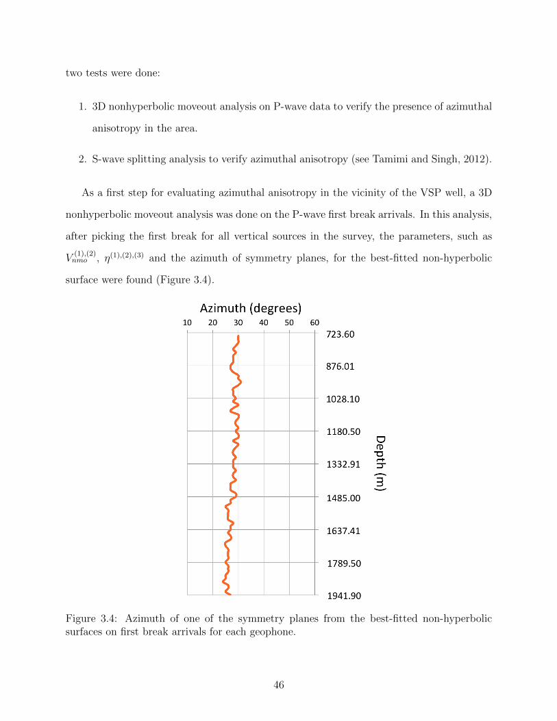
two tests were done:

1. 3D nonhyperbolic moveout analysis on P-wave data to verify the presence of azimuthal

anisotropy in the area.

2. S-wave splitting analysis to verify azimuthal anisotropy (see Tamimi and Singh, 2012).

As a first step for evaluating azimuthal anisotropy in the vicinity of the VSP well, a 3D

nonhyperbolic moveout analysis was done on the P-wave first break arrivals. In this analysis,

after picking the first break for all vertical sources in the survey, the parameters, such as

V(1),(2)nmo , η(1),(2),(3) and the azimuth of symmetry planes, for the best-fitted non-hyperbolic

surface were found (Figure 3.4).

Figure 3.4: Azimuth of one of the symmetry planes from the best-fitted non-hyperbolicsurfaces on first break arrivals for each geophone.

46

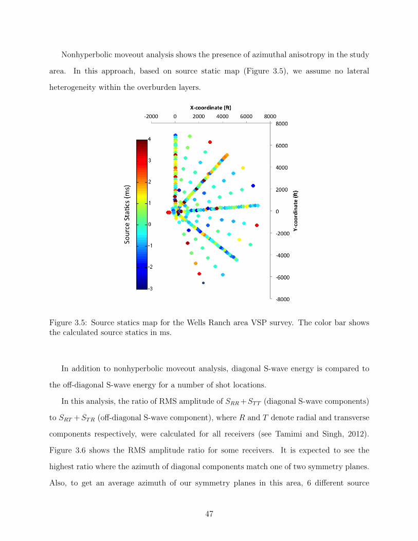
Nonhyperbolic moveout analysis shows the presence of azimuthal anisotropy in the study

area. In this approach, based on source static map (Figure 3.5), we assume no lateral

heterogeneity within the overburden layers.

Figure 3.5: Source statics map for the Wells Ranch area VSP survey. The color bar showsthe calculated source statics in ms.

In addition to nonhyperbolic moveout analysis, diagonal S-wave energy is compared to

the off-diagonal S-wave energy for a number of shot locations.

In this analysis, the ratio of RMS amplitude of SRR+STT (diagonal S-wave components)

to SRT +STR (off-diagonal S-wave component), where R and T denote radial and transverse

components respectively, were calculated for all receivers (see Tamimi and Singh, 2012).

Figure 3.6 shows the RMS amplitude ratio for some receivers. It is expected to see the

highest ratio where the azimuth of diagonal components match one of two symmetry planes.

Also, to get an average azimuth of our symmetry planes in this area, 6 different source

47

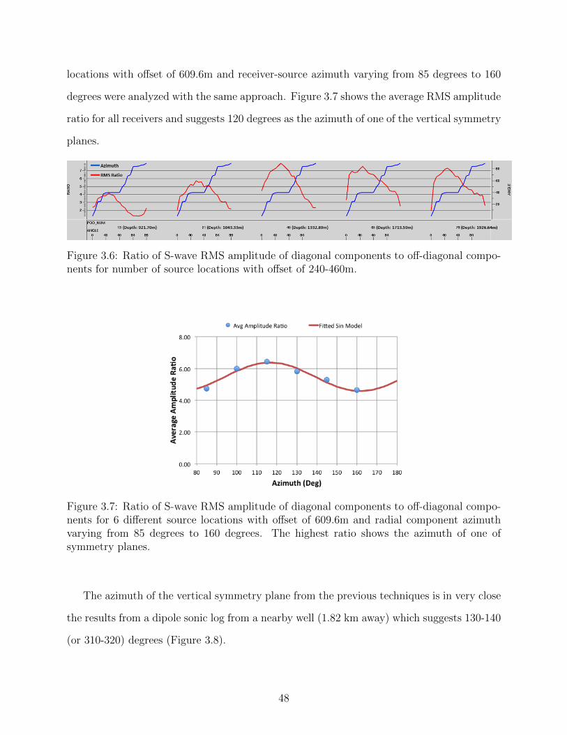
locations with offset of 609.6m and receiver-source azimuth varying from 85 degrees to 160

degrees were analyzed with the same approach. Figure 3.7 shows the average RMS amplitude

ratio for all receivers and suggests 120 degrees as the azimuth of one of the vertical symmetry

planes.

Figure 3.6: Ratio of S-wave RMS amplitude of diagonal components to off-diagonal compo-nents for number of source locations with offset of 240-460m.

Figure 3.7: Ratio of S-wave RMS amplitude of diagonal components to off-diagonal compo-nents for 6 different source locations with offset of 609.6m and radial component azimuthvarying from 85 degrees to 160 degrees. The highest ratio shows the azimuth of one ofsymmetry planes.

The azimuth of the vertical symmetry plane from the previous techniques is in very close

the results from a dipole sonic log from a nearby well (1.82 km away) which suggests 130-140

(or 310-320) degrees (Figure 3.8).

48

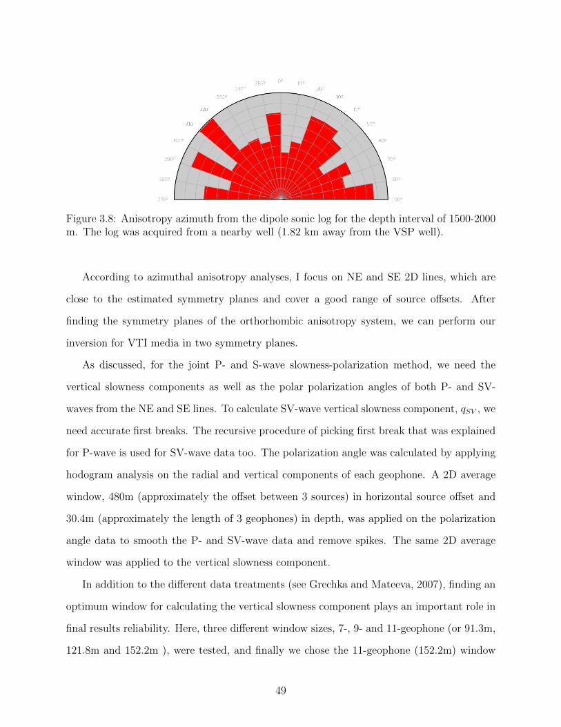
Figure 3.8: Anisotropy azimuth from the dipole sonic log for the depth interval of 1500-2000m. The log was acquired from a nearby well (1.82 km away from the VSP well).

According to azimuthal anisotropy analyses, I focus on NE and SE 2D lines, which are

close to the estimated symmetry planes and cover a good range of source offsets. After

finding the symmetry planes of the orthorhombic anisotropy system, we can perform our

inversion for VTI media in two symmetry planes.

As discussed, for the joint P- and S-wave slowness-polarization method, we need the

vertical slowness components as well as the polar polarization angles of both P- and SV-

waves from the NE and SE lines. To calculate SV-wave vertical slowness component, qSV , we

need accurate first breaks. The recursive procedure of picking first break that was explained

for P-wave is used for SV-wave data too. The polarization angle was calculated by applying

hodogram analysis on the radial and vertical components of each geophone. A 2D average

window, 480m (approximately the offset between 3 sources) in horizontal source offset and

30.4m (approximately the length of 3 geophones) in depth, was applied on the polarization

angle data to smooth the P- and SV-wave data and remove spikes. The same 2D average

window was applied to the vertical slowness component.

In addition to the different data treatments (see Grechka and Mateeva, 2007), finding an

optimum window for calculating the vertical slowness component plays an important role in

final results reliability. Here, three different window sizes, 7-, 9- and 11-geophone (or 91.3m,

121.8m and 152.2m ), were tested, and finally we chose the 11-geophone (152.2m) window

49

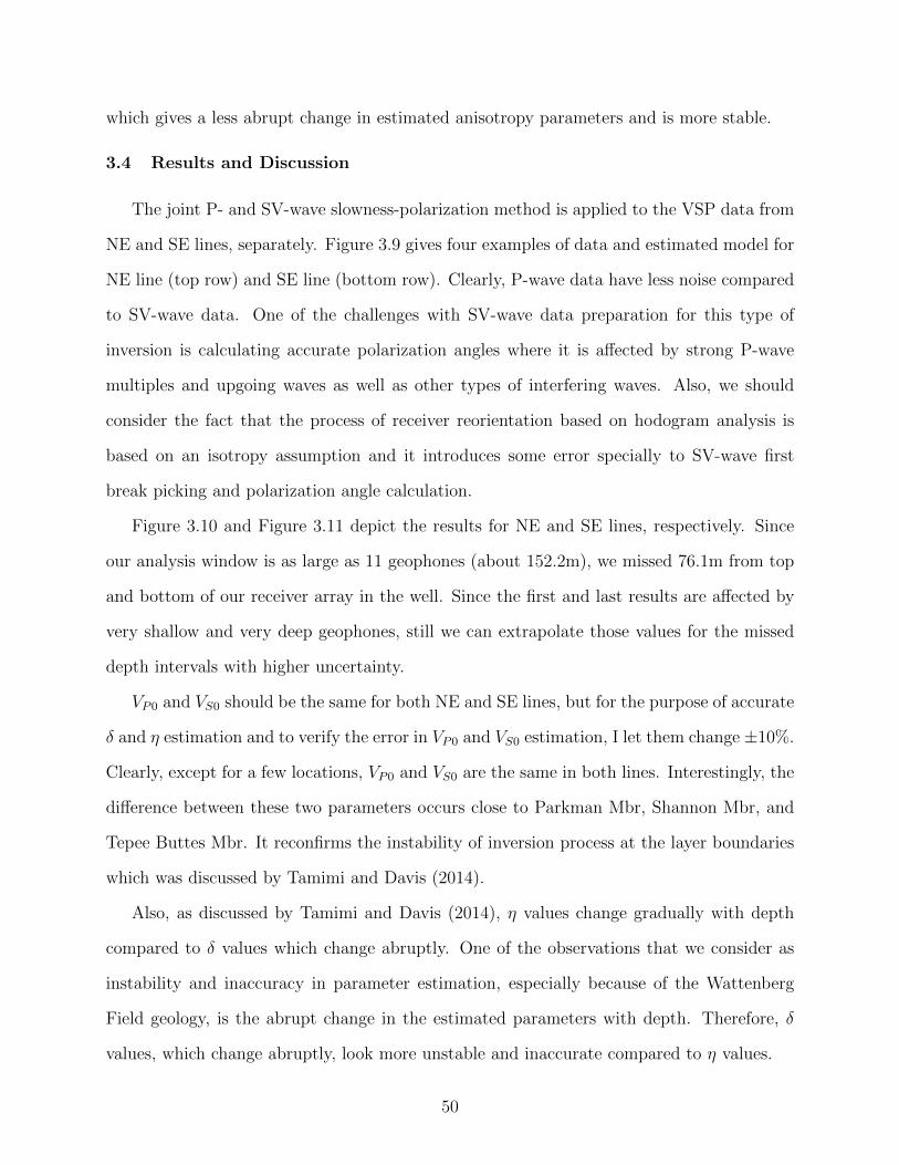
which gives a less abrupt change in estimated anisotropy parameters and is more stable.


The joint P- and SV-wave slowness-polarization method is applied to the VSP data from

NE and SE lines, separately. Figure 3.9 gives four examples of data and estimated model for

NE line (top row) and SE line (bottom row). Clearly, P-wave data have less noise compared

to SV-wave data. One of the challenges with SV-wave data preparation for this type of

inversion is calculating accurate polarization angles where it is affected by strong P-wave

multiples and upgoing waves as well as other types of interfering waves. Also, we should

consider the fact that the process of receiver reorientation based on hodogram analysis is

based on an isotropy assumption and it introduces some error specially to SV-wave first

break picking and polarization angle calculation.

Figure 3.10 and Figure 3.11 depict the results for NE and SE lines, respectively. Since

our analysis window is as large as 11 geophones (about 152.2m), we missed 76.1m from top

and bottom of our receiver array in the well. Since the first and last results are affected by

very shallow and very deep geophones, still we can extrapolate those values for the missed

depth intervals with higher uncertainty.

VP0 and VS0 should be the same for both NE and SE lines, but for the purpose of accurate

δ and η estimation and to verify the error in VP0 and VS0 estimation, I let them change ±10%.

Clearly, except for a few locations, VP0 and VS0 are the same in both lines. Interestingly, the

difference between these two parameters occurs close to Parkman Mbr, Shannon Mbr, and

Tepee Buttes Mbr. It reconfirms the instability of inversion process at the layer boundaries

which was discussed by Tamimi and Davis (2014).

Also, as discussed by Tamimi and Davis (2014), η values change gradually with depth

compared to δ values which change abruptly. One of the observations that we consider as

instability and inaccuracy in parameter estimation, especially because of the Wattenberg

Field geology, is the abrupt change in the estimated parameters with depth. Therefore, δ

values, which change abruptly, look more unstable and inaccurate compared to η values.

50

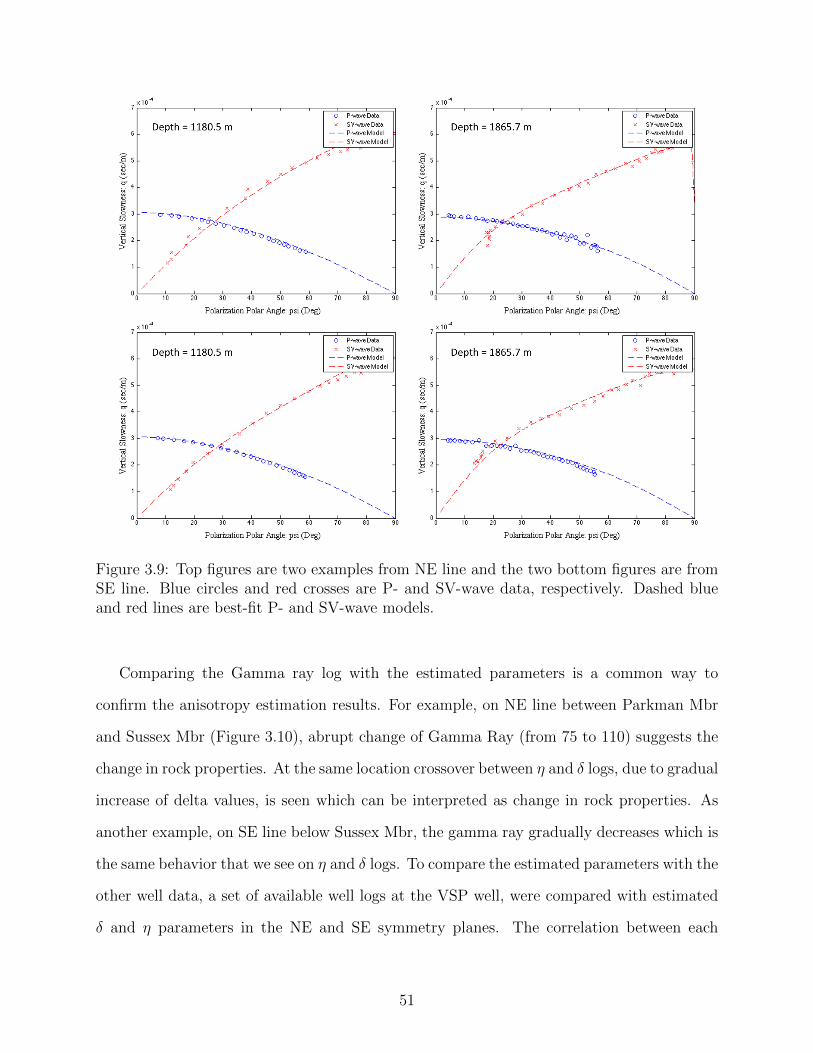
Figure 3.9: Top figures are two examples from NE line and the two bottom figures are fromSE line. Blue circles and red crosses are P- and SV-wave data, respectively. Dashed blueand red lines are best-fit P- and SV-wave models.

Comparing the Gamma ray log with the estimated parameters is a common way to

confirm the anisotropy estimation results. For example, on NE line between Parkman Mbr

and Sussex Mbr (Figure 3.10), abrupt change of Gamma Ray (from 75 to 110) suggests the

change in rock properties. At the same location crossover between η and δ logs, due to gradual

increase of delta values, is seen which can be interpreted as change in rock properties. As

another example, on SE line below Sussex Mbr, the gamma ray gradually decreases which is

the same behavior that we see on η and δ logs. To compare the estimated parameters with the

other well data, a set of available well logs at the VSP well, were compared with estimated

δ and η parameters in the NE and SE symmetry planes. The correlation between each

51

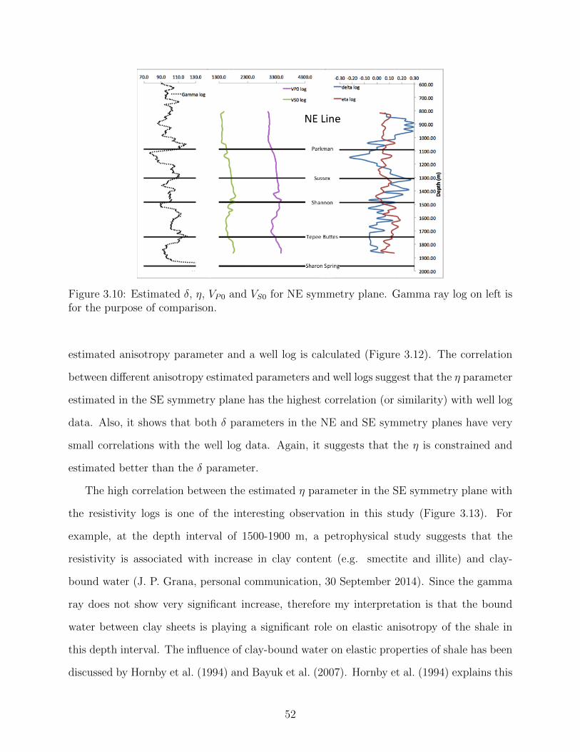
Figure 3.10: Estimated δ, η, VP0 and VS0 for NE symmetry plane. Gamma ray log on left isfor the purpose of comparison.

estimated anisotropy parameter and a well log is calculated (Figure 3.12). The correlation

between different anisotropy estimated parameters and well logs suggest that the η parameter

estimated in the SE symmetry plane has the highest correlation (or similarity) with well log

data. Also, it shows that both δ parameters in the NE and SE symmetry planes have very

small correlations with the well log data. Again, it suggests that the η is constrained and

estimated better than the δ parameter.

The high correlation between the estimated η parameter in the SE symmetry plane with

the resistivity logs is one of the interesting observation in this study (Figure 3.13). For

example, at the depth interval of 1500-1900 m, a petrophysical study suggests that the

resistivity is associated with increase in clay content (e.g. smectite and illite) and clay-

bound water (J. P. Grana, personal communication, 30 September 2014). Since the gamma

ray does not show very significant increase, therefore my interpretation is that the bound

water between clay sheets is playing a significant role on elastic anisotropy of the shale in

this depth interval. The influence of clay-bound water on elastic properties of shale has been

discussed by Hornby et al. (1994) and Bayuk et al. (2007). Hornby et al. (1994) explains this

52

Figure 3.11: Estimated δ, η, VP0 and VS0 for SE symmetry plane. Gamma ray log on left isfor the purpose of comparison.

phenomena by defining ”clay-water composites” which are packages of clay sheets separated

by bound water and with significant elastic anisotropic properties (Figure 3.14). In addition

to significant elastic properties, these clay-water composites have high electrical conductivity.

Therefore, we see high correlation between the estimated eta and the resistivity log. In

addition to the resistivity log, in the shallow part of the well (around 1000m), we see a good

correlation between the estimated η and the density log, too (Figure 3.13).

To verify the advantage of joint P- and S-wave method compared to P-wave method, the

estimation process with the same data and parameter was done using P-wave data only for

NE line. The results for the slowness-polarization method using P-wave data only approach

are shown in Figure 3.15. Clearly, the joint method constrains anisotropy parameters, espe-

cially the δ parameter, better than the P-wave only approach. The results of P-wave only

method clearly depict dramatic change in δ values, while we don’t see such a behavior for η

values. Thus, involving S-wave data is crucial when an accurate δ estimation is needed.

53

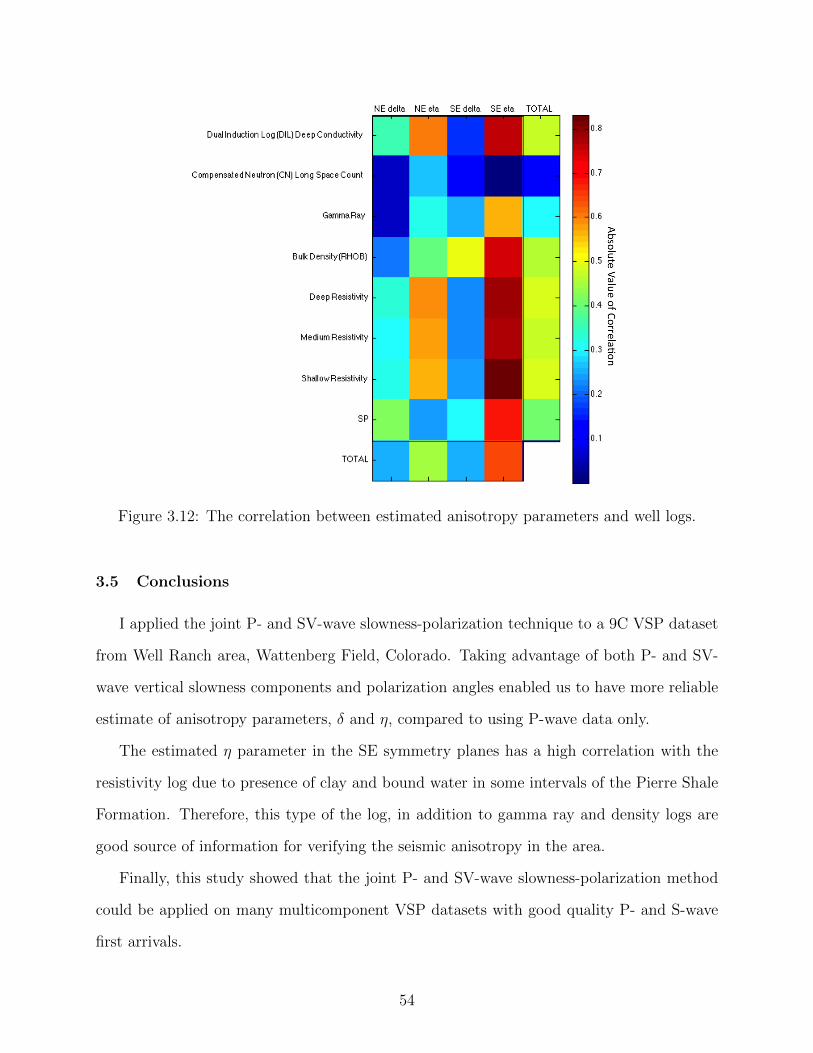
Figure 3.12: The correlation between estimated anisotropy parameters and well logs.

3.5 Conclusions

I applied the joint P- and SV-wave slowness-polarization technique to a 9C VSP dataset

from Well Ranch area, Wattenberg Field, Colorado. Taking advantage of both P- and SV-

wave vertical slowness components and polarization angles enabled us to have more reliable

estimate of anisotropy parameters, δ and η, compared to using P-wave data only.

The estimated η parameter in the SE symmetry planes has a high correlation with the

resistivity log due to presence of clay and bound water in some intervals of the Pierre Shale

Formation. Therefore, this type of the log, in addition to gamma ray and density logs are

good source of information for verifying the seismic anisotropy in the area.

Finally, this study showed that the joint P- and SV-wave slowness-polarization method

could be applied on many multicomponent VSP datasets with good quality P- and S-wave

first arrivals.

54

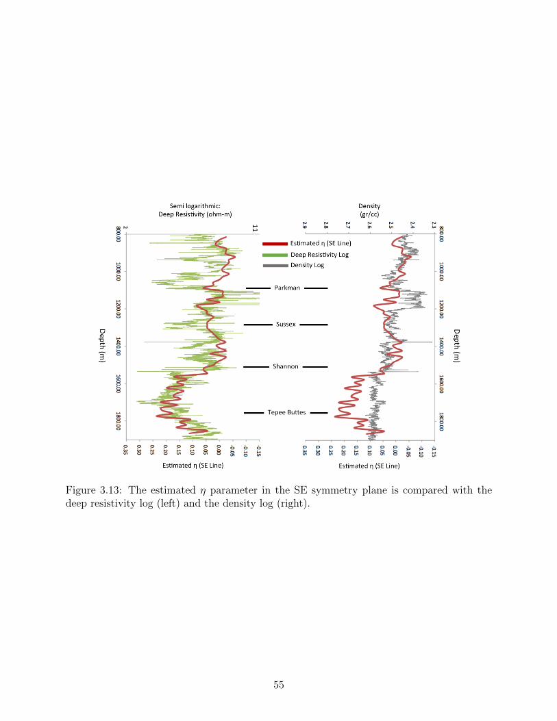
Figure 3.13: The estimated η parameter in the SE symmetry plane is compared with thedeep resistivity log (left) and the density log (right).

55

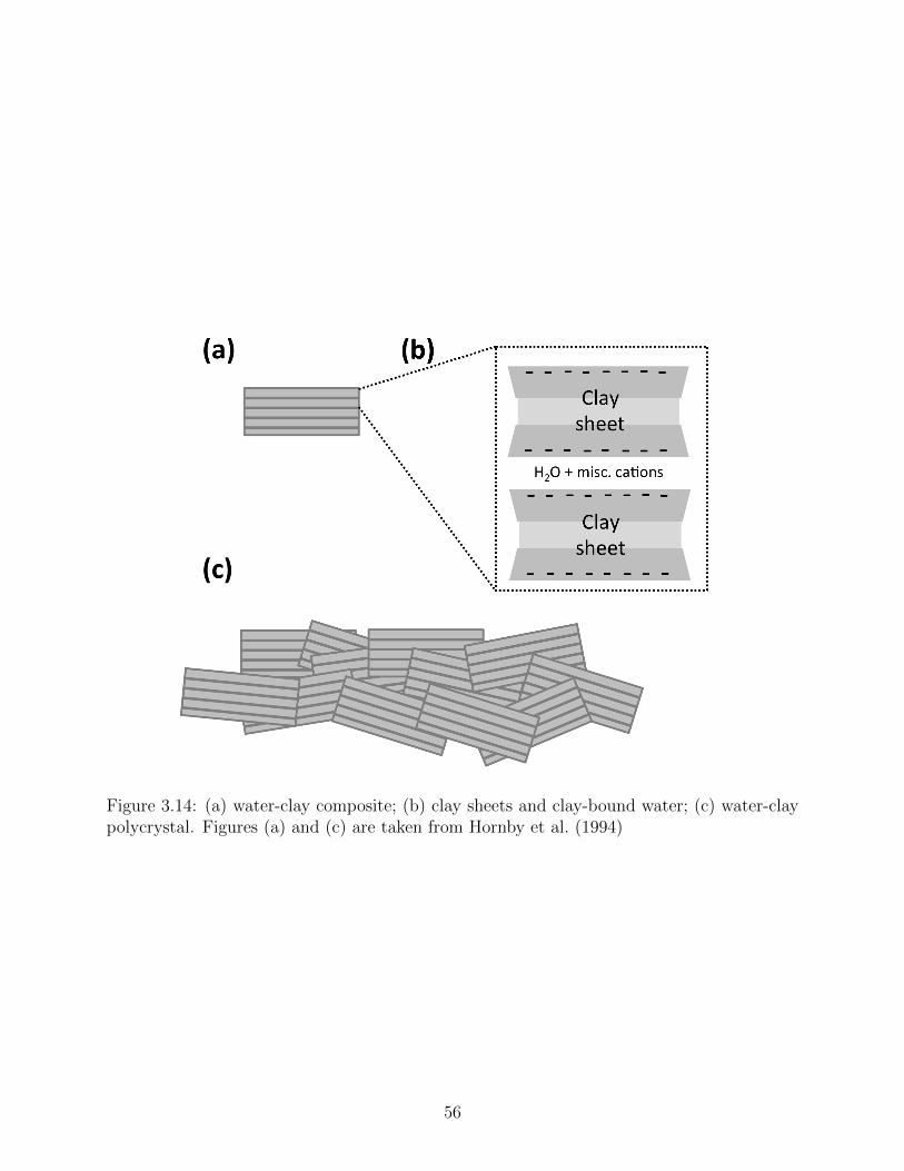
Figure 3.14: (a) water-clay composite; (b) clay sheets and clay-bound water; (c) water-claypolycrystal. Figures (a) and (c) are taken from Hornby et al. (1994)

56

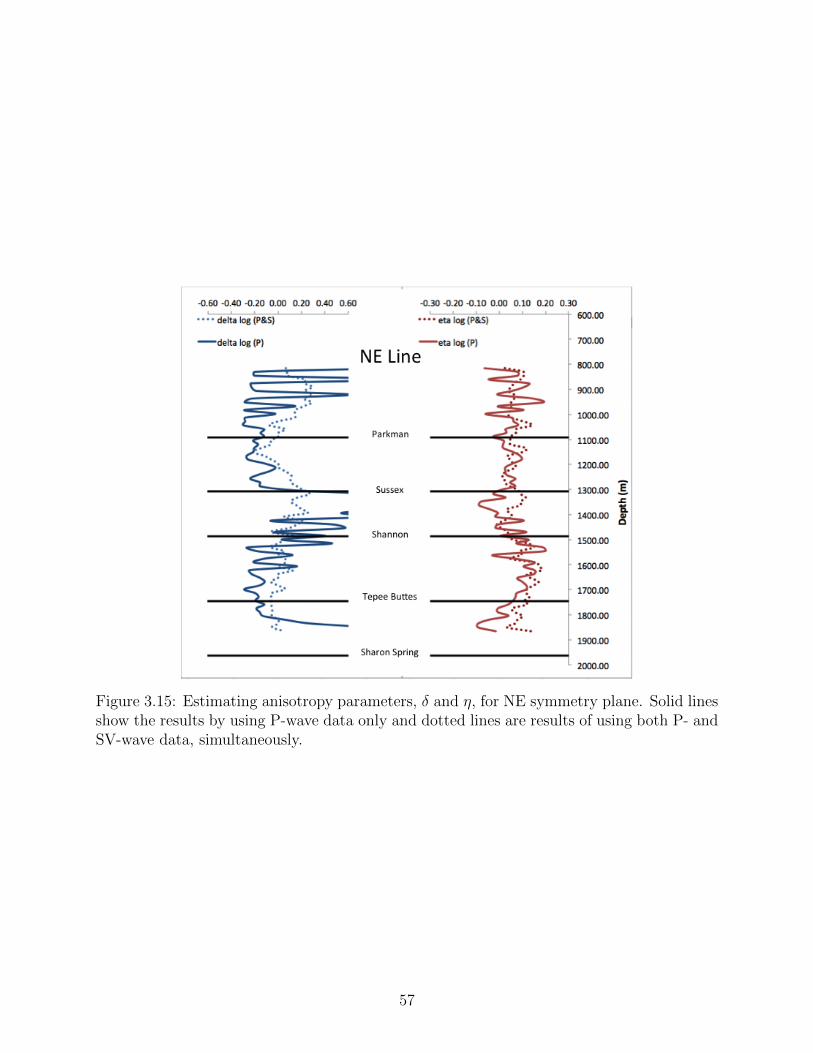
Figure 3.15: Estimating anisotropy parameters, δ and η, for NE symmetry plane. Solid linesshow the results by using P-wave data only and dotted lines are results of using both P- andSV-wave data, simultaneously.

57

CHAPTER 4

PRESTACK WAVEFORM INVERSION OF MULTICOMPONENT VSP DATA FOR

ESTIMATING ORTHORHOMBIC ANISOTROPY PARAMETERS AT THE WELLS

RANCH AREA, WATTENBERG FIELD, COLORADO

In Chapter 3, the anisotropy parameters δ and η in two vertical symmetry planes of

orthorhombic media were inferred from a VSP dataset from Wells Ranch at Wattenberg

Field, Colorado. The technique for estimating the anisotropy parameters was the joint P-

and SV-wave slowness-polarization method that is needed to be calibrated through a different

approach. Waveform inversion is one of the techniques that can be used for calibrating

the results of the joint slowness-polarization method. Using multicomponent VSP data

and a novel approach in waveform inversion, the orthorhombic anisotropy parameters were

estimated and compared with the results of the joint slowness-polarization method. This

chapter is a research collaboration with Tao Li from University of Wyoming. This research

is the first attempt to apply this approach to real field VSP data. Processing and preparing

the P- and S-wave data for the waveform inversion and comparison between the results of

two methods are my contributions to this research.

4.1 Introduction

Exploring and characterizing naturally fractured reservoirs and unconventional resources

has triggered an increased interest in azimuthal anisotropy analysis. Inverting seismic data

for characterizing horizontal transverse isotropy (HTI), tilted transverse isotropy (TTI) and

orthorhombic anisotropy systems in earth subsurface has been the subject of many publi-

cations these years. Many of the proposed methodologies take advantage of multicompo-

nent seismic data for this purpose. Successful results of characterizing subsurface elastic

parameters in VTI media using prestack waveform inversion (Kamath and Tsvankin, 2013;

58

Padhi and Mallick, 2013) encouraged many researchers to apply the technique to azimuthally

anisotropic media (Li and Mallick, 2013).

Prestack waveform inversion, also called full waveform inversion (FWI) or waveform to-

mography, is a process of inferring earth model parameters (e.g. density, velocity, anisotropy

and attenuation) by minimizing the difference between data acquired in the field and the

synthetic data using forward modeling (Brittan et al., 2013). Virieux and Opetro (2009)

reviewed different theoretical and application aspects of the waveform inversion in details,

and we only focus on a new development on the technique and its results.

One of the challenges for performing the waveform inversion is the way to handle objec-

tive functions. Generally, there are two approaches to overcome this problem and perform

prestack waveform inversion in complex media such as orthorhombic media: 1) defining a

single objective function, which is a weighted sum of the objective functions of the individual

data components, and 2) applying multiobjective optimization algorithm (Li and Mallick,

2013). In the first approach, finding optimal weights for each component is nontrivial and

the results depend on user’s choice. The second approach suffers from nonlinear problem

challenges and nonunique or multiple optimal solutions. To overcome the issues associated

with the second approach, Li and Mallick (2013) suggested implementing nondominated

sorting genetic algorithm II (NSGA II) (Deb et al., 2002) in the prestack waveform inversion

of multicomponent seismic data.

4.2 Methodology

Many real-world problems are multiple objective problems. In a multiple objective prob-

lem, a set of optimal solutions satisfies a set of defined objective functions, and none of

the solutions, commonly called Pareto-optimal solutions, is better than the others without

further information (Deb et al., 2002). Different multiobjective optimization algorithms at-

tempt to find optimal solutions through minimum computations. One of the popular and

successful methods is NSGA II proposed by Deb et al. (2002). NSGA II is an elitist mul-

tiobjective evolutionary algorithm (MOEA) which utilize a fast nondominated sorting and

59

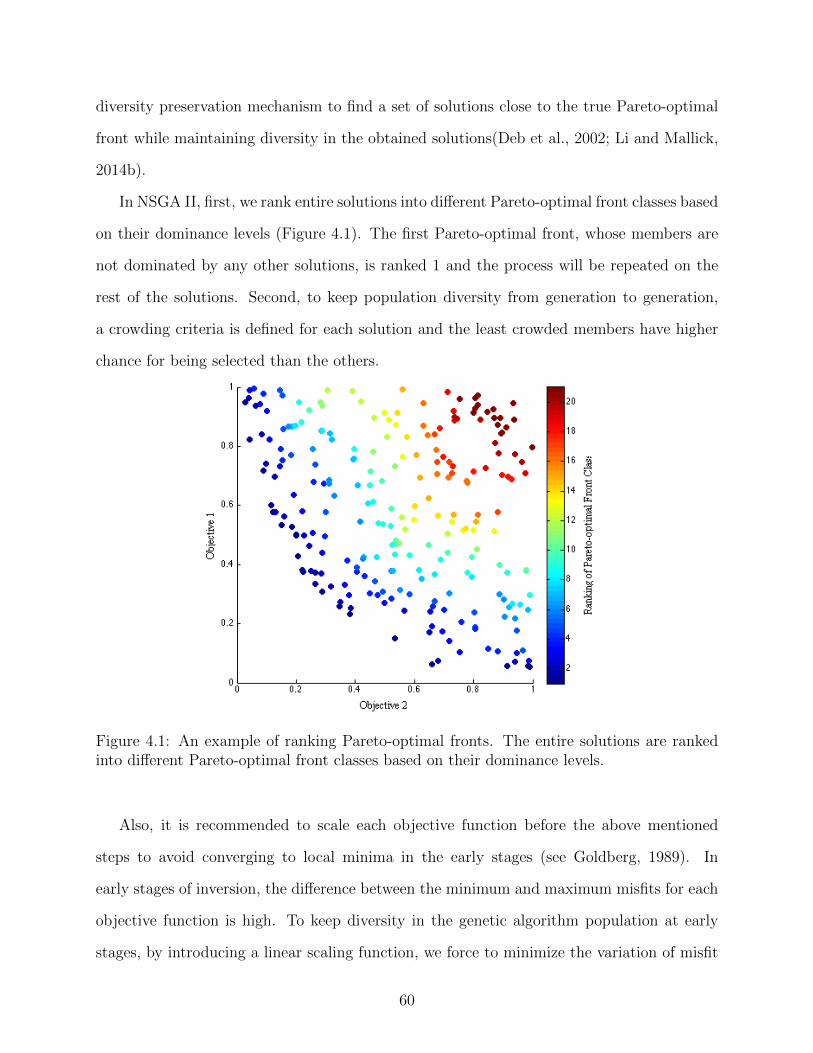
diversity preservation mechanism to find a set of solutions close to the true Pareto-optimal

front while maintaining diversity in the obtained solutions(Deb et al., 2002; Li and Mallick,

2014b).

In NSGA II, first, we rank entire solutions into different Pareto-optimal front classes based

on their dominance levels (Figure 4.1). The first Pareto-optimal front, whose members are

not dominated by any other solutions, is ranked 1 and the process will be repeated on the

rest of the solutions. Second, to keep population diversity from generation to generation,

a crowding criteria is defined for each solution and the least crowded members have higher

chance for being selected than the others.

Figure 4.1: An example of ranking Pareto-optimal fronts. The entire solutions are rankedinto different Pareto-optimal front classes based on their dominance levels.

Also, it is recommended to scale each objective function before the above mentioned

steps to avoid converging to local minima in the early stages (see Goldberg, 1989). In

early stages of inversion, the difference between the minimum and maximum misfits for each

objective function is high. To keep diversity in the genetic algorithm population at early

stages, by introducing a linear scaling function, we force to minimize the variation of misfit

60

for each objective function. As generation progresses and the inversion process passes early

stages, the difference between minimum and maximum misfits for each objective function

becomes smaller and we can relax the scaling process. At least, there are two popular scaling

processes: linear scaling and exponential scaling (Li and Mallick, 2014a). Experiments by Li

and Mallick (2014a) suggest that for anisotropic waveform inversion, scaling linear objective

functions linearly avoid premature convergence.

The main challenge of NSGA II, and many stochastic optimization algorithms, is compu-

tational complexity. For example NSGA II has computational complexity of O(MN2), where

M is the number of objective functions and N is the population size. For an azimuthally

anisotropic seismic inversion problem, maintaining a large population size is necessary and

it results in high computational complexity and expenses. The main reason computational

complexity of for NSGA II is due to the nondominated sorting procedure. Li and Mallick

(2014b) developed a parallel version of the original NSGA II algorithm to handle complex

problems such as prestack waveform inversion of seismic data in anisotropic media (Fig-

ure 4.2). Currently, the methodology is developed for estimating 1D subsurface elastic model

from surface seismic and VSP data.

4.3 Review of the Dataset

The above mentioned methodology can be applied on surface seismic and borehole seis-

mic data. Here we use multicomponent VSP survey from the Well Ranch area that was

presented in Chapter 3. Although full 9C data are available, we used the 3 component data

recorded from vertical source and perform the waveform inversion with the above mentioned

methodology. Waveform inversion on 9C VSP data requires additional data processing and

more computational time which is out of the scope and time of this research. Also, four full

offset 2D lines in N, NE, E and SE directions are selected for the inversion (Figure 4.3).

61

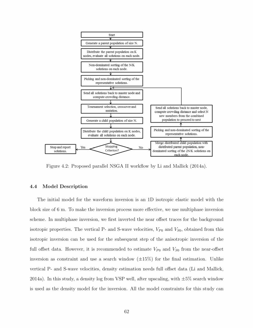
Figure 4.2: Proposed parallel NSGA II workflow by Li and Mallick (2014a).

4.4 Model Description

The initial model for the waveform inversion is an 1D isotropic elastic model with the

block size of 6 m. To make the inversion process more effective, we use multiphase inversion

scheme. In multiphase inversion, we first inverted the near offset traces for the background

isotropic properties. The vertical P- and S-wave velocities, VP0 and VS0, obtained from this

isotropic inversion can be used for the subsequent step of the anisotropic inversion of the

full offset data. However, it is recommended to estimate VP0 and VS0 from the near-offset

inversion as constraint and use a search window (±15%) for the final estimation. Unlike

vertical P- and S-wave velocities, density estimation needs full offset data (Li and Mallick,

2014a). In this study, a density log from VSP well, after upscaling, with ±5% search window

is used as the density model for the inversion. All the model constraints for this study can

62

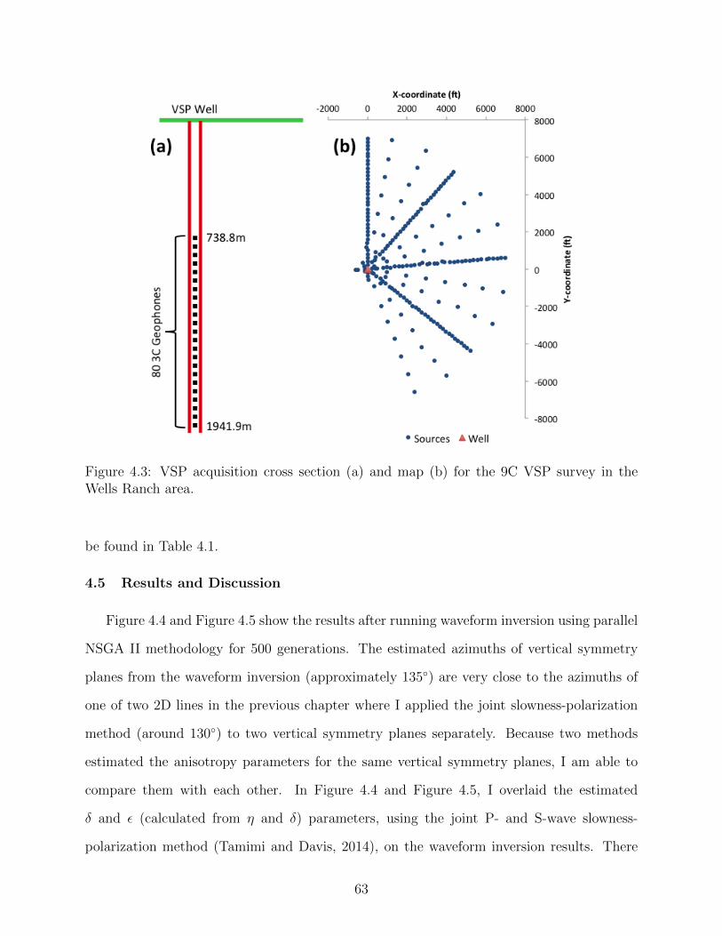
Figure 4.3: VSP acquisition cross section (a) and map (b) for the 9C VSP survey in theWells Ranch area.

be found in Table 4.1.


Figure 4.4 and Figure 4.5 show the results after running waveform inversion using parallel

NSGA II methodology for 500 generations. The estimated azimuths of vertical symmetry

planes from the waveform inversion (approximately 135◦) are very close to the azimuths of

one of two 2D lines in the previous chapter where I applied the joint slowness-polarization

method (around 130◦) to two vertical symmetry planes separately. Because two methods

estimated the anisotropy parameters for the same vertical symmetry planes, I am able to

compare them with each other. In Figure 4.4 and Figure 4.5, I overlaid the estimated

δ and ε (calculated from η and δ) parameters, using the joint P- and S-wave slowness-

polarization method (Tamimi and Davis, 2014), on the waveform inversion results. There

63

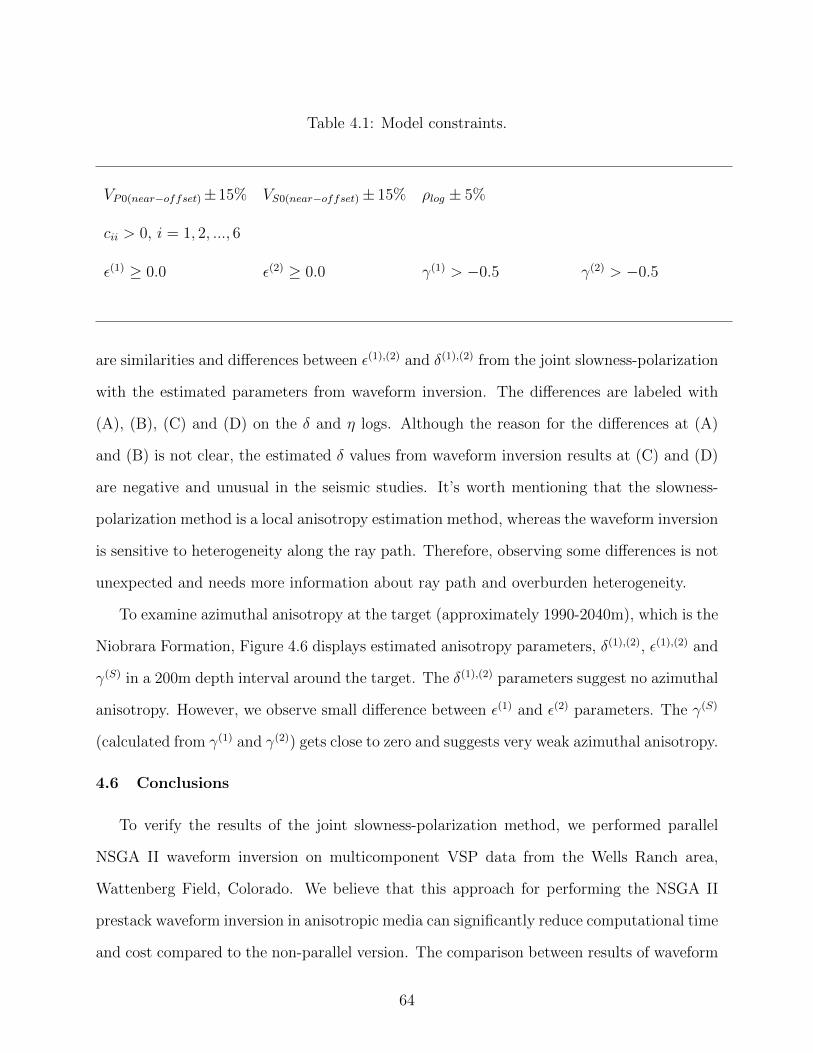
Table 4.1: Model constraints.

VP0(near−offset)±15% VS0(near−offset)± 15% ρlog ± 5%

cii > 0, i = 1, 2, ..., 6

ε(1) ≥ 0.0 ε(2) ≥ 0.0 γ(1) > −0.5 γ(2) > −0.5

are similarities and differences between ε(1),(2) and δ(1),(2) from the joint slowness-polarization

with the estimated parameters from waveform inversion. The differences are labeled with

(A), (B), (C) and (D) on the δ and η logs. Although the reason for the differences at (A)

and (B) is not clear, the estimated δ values from waveform inversion results at (C) and (D)

are negative and unusual in the seismic studies. It’s worth mentioning that the slowness-

polarization method is a local anisotropy estimation method, whereas the waveform inversion

is sensitive to heterogeneity along the ray path. Therefore, observing some differences is not

unexpected and needs more information about ray path and overburden heterogeneity.

To examine azimuthal anisotropy at the target (approximately 1990-2040m), which is the

Niobrara Formation, Figure 4.6 displays estimated anisotropy parameters, δ(1),(2), ε(1),(2) and

γ(S) in a 200m depth interval around the target. The δ(1),(2) parameters suggest no azimuthal

anisotropy. However, we observe small difference between ε(1) and ε(2) parameters. The γ(S)

(calculated from γ(1) and γ(2)) gets close to zero and suggests very weak azimuthal anisotropy.

4.6 Conclusions

To verify the results of the joint slowness-polarization method, we performed parallel

NSGA II waveform inversion on multicomponent VSP data from the Wells Ranch area,

Wattenberg Field, Colorado. We believe that this approach for performing the NSGA II

prestack waveform inversion in anisotropic media can significantly reduce computational time

and cost compared to the non-parallel version. The comparison between results of waveform

64

inversion and the joint slowness-polarization method, close to the VSP well, reveals ε(1),(2)

and δ(1),(2), are similar for some depth intervals. Also the results of the waveform inversion

suggests that δ(1) and δ(2) values are very close and ε(1) and ε(2) are slightly different at top

of the Niobrara Formation. Therefore, we expect weak azimuthal anisotropy at the Niobrara

Formation close to the VSP well.

65

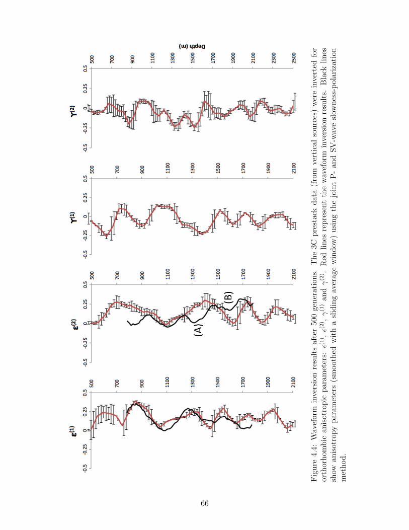
Fig

ure

4.4:

Wav

efor

min

vers

ion

resu

lts

afte

r50

0ge

ner

atio

ns.

The

3Cpre

stac

kdat

a(f

rom

vert

ical

sourc

es)

wer

ein

vert

edfo

ror

thor

hom

bic

anis

otro

pic

par

amet

ers:ε(

1) ,ε(

2) ,γ(1)

andγ(2) .

Red

lines

repre

sent

the

wav

efor

min

vers

ion

resu

lts.

Bla

cklines

show

anis

otro

py

par

amet

ers

(sm

oot

hed

wit

ha

slid

ing

aver

age

win

dow

)usi

ng

the

join

tP

-an

dSV

-wav

esl

ownes

s-p

olar

izat

ion

met

hod.

66

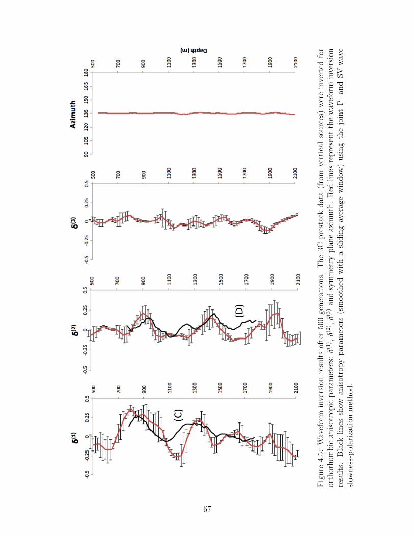
Fig

ure

4.5:

Wav

efor

min

vers

ion

resu

lts

afte

r50

0ge

ner

atio

ns.

The

3Cpre

stac

kdat

a(f

rom

vert

ical

sourc

es)

wer

ein

vert

edfo

ror

thor

hom

bic

anis

otro

pic

par

amet

ers:δ(

1) ,δ(

2) ,δ(

3)

and

sym

met

rypla

ne

azim

uth

.R

edlines

repre

sent

the

wav

efor

min

vers

ion

resu

lts.

Bla

cklines

show

anis

otro

py

par

amet

ers

(sm

oot

hed

wit

ha

slid

ing

aver

age

win

dow

)usi

ng

the

join

tP

-an

dSV

-wav

esl

ownes

s-p

olar

izat

ion

met

hod.

67

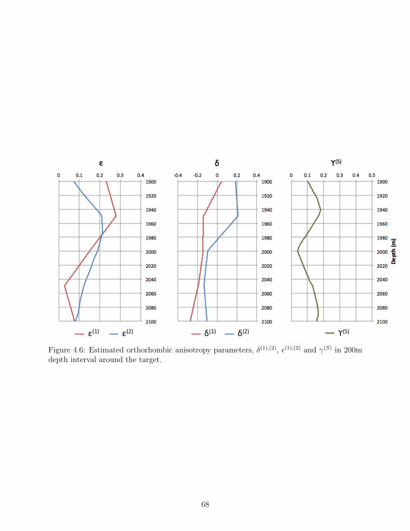
Figure 4.6: Estimated orthorhombic anisotropy parameters, δ(1),(2), ε(1),(2) and γ(S) in 200mdepth interval around the target.

68

CHAPTER 5

APPLICATIONS OF THE ANISOTROPIC VELOCITY MODEL OBTAINED FROM

JOINT SLOWNESS-POLARIZATION METHOD IN PRE- AND POST-STACK VSP

DATA ANALYSES

The higher signal-to-noise ratio of VSP data compared to surface seismic data makes

them suitable for amplitude-related analyses and reflection seismic imaging. However, some-

times removing undesirable effects from the amplitude information is necessary. Geometrical

spreading is one of the effects that should be removed before amplitude analysis and imaging,

and it needs special considerations, where the subsurface medium is anisotropic.

One of the successful surface seismic techniques to compensate for amplitude distortion

due to geometrical spreading is MASC (Moveout-Based Anisotropic Spreading Correction).

We modified this technique for VSP data, and applied the modified technique to the VSP

data from the Wells Ranch area at Wattenberg Field, CO. The AVO responses from top of

the reservoir in two symmetry planes were analyzed.

The AVO response from top of the Niobrara Formation shows weak azimuthal anisotropy,

which is consistent with previous studies on surface seismic data and production history.

Finally, using the anisotropic velocity model from the joint slowness-polarization method,

the Niobrara Formation is imaged. The seismic image after anisotropic VSP-CDP transfor-

mation shows improvement compared to the isotropic image.

5.1 Introduction

The approaches for analyzing seismic data can be divided into two classes: amplitude

methods and traveltime methods. Normally, amplitude methods have higher vertical res-

olution compared to traveltime methods, which makes them suitable for thin reservoirs

(Tsvankin and Grechka, 2011; Xu et al., 2005). Prestack amplitude variation with offset

(AVO) and azimuth (azimuthal AVO or AVAZ) is a well known amplitude method, which

69

provides essential information for characterizing subsurface fractures and in-situ stress field

(e.g. DeVault et al., 2002; Mallick et al., 1998; Ramos and Davis, 1997). Although AVO and

AVAZ aim to analyze amplitude variation due to reflection coefficient variation, different fac-

tors such as source radiation pattern, geometrical spreading, attenuation, transmission, and

the conversion coefficients at the receiver change the amplitude dramatically along raypath

too (Martinez, 1993; Maultzsch et al., 2003; Xu et al., 2005). Those factors also directly

affect final seismic image quality.

Hence the effect of the above mentioned factors should be removed before prestack am-

plitude analysis. Among the mentioned factors, attenuation and geometrical spreading have

the most significant effects on amplitude. Here, we compensate for the attenuation effect

by approximating the effective Q factor using the spectral ratio method. In addition to

attenuation, the geometrical spreading effect should be removed, which is the main scope of

this research.

Dynamic ray tracing (Gajewski and Psencık, 1990) and moveout-based anisotropic spread-

ing correction (MASC) (Xu and Tsvankin, 2006; Xu et al., 2005) are two options for removing

the geometrical spreading effect from the surface seismic data in anisotropic media. While

dynamic ray tracing is time consuming and requires accurate subsurface velocity information

(Tsvankin and Grechka, 2011), MASC technique is fast and requires the effective moveout

parameters, which can be derived from traveltime data directly.

Because the MASC by Xu et al. (2005) has been developed for surface seismic geometry,

applying the same methodology to VSP geometry requires some modifications. In this paper,

we explain applying the MASC technique to the P-wave data from VSP geometry. In this

approach, for each source and receiver in the VSP well, we need a velocity model to find the

location of corresponding pseudo-receiver on the ground. Because we don’t use the velocity

model information to correct the amplitude directly, the velocity model in this approach

does not need to be as accurate as the velocity model for performing dynamic ray tracing.

We used the results of the joint P- and SV-wave slowness-polarization technique (Tamimi

70

and Davis, 2014), for building the overburden anisotropic velocity model.

5.2 Theory of MASC

As an elastic wave propagates away from the source, the amplitude decays due to the

wavefront expansion, which is called geometrical spreading. The ray-theory Green’s function

Gin (see Cerveny, 2001) shows the role of the relative geometrical spreading L(R, S) between

the source S and the receiver R.

Gin(R, t;S, t0) =gn(S)gi(R)eiT

G(R,S)

4π[ρ(S)ρ(R)V (S)V (R)]1/2L(R, S)×RCδ(t− t0 − T (R, S)), (5.1)

where t0 and t are the excitation and recording times, ρ(S), V (S), ρ(R), and V (R) are

densities and phase velocities at the source (S) and receiver (R), respectively. gn(S) and

gn(R) are the polarization vectors at the source and receiver, TG(R, S) is the complete phase

shift, RC is the product of the reflection/transmission coefficients normalized with respect

to the vertical energy flux at all interfaces crossed by the ray, δ(t) is delta function, and

T (R, S) is the traveltime. As mentioned, L(R, S) (Cerveny, 2001), is the relative geometrical

spreading, which can be rewritten in the following function of traveltime T for non-converted

wave modes in laterally homogeneous media (Tsvankin and Grechka, 2011):

L(R, S) = L(x, α) =√

cosφs cosφr x

∣∣∣∣∣∂2T∂x2(∂2T

∂α2+ x

∂T

∂x

)−(∂2T

∂x∂α− 1

x

∂T

∂α

)2∣∣∣∣∣− 1

2

, (5.2)

where x is the source-receiver offset, α is the azimuth of the source-receiver line, φs and

φr are the angles between the ray and the vertical at the source and receiver, respectively,

and T is the traveltime.

For laterally homogenous orthorhombic media with a horizontal symmetry plane, where

φs = φr = φ, equation 5.2 simplifies to

L(R, S) = L(x, α) = cosφ x

∣∣∣∣∣∂2T∂x2(∂2T

∂α2+ x

∂T

∂x

)−(∂2T

∂x∂α− 1

x

∂T

∂α

)2∣∣∣∣∣− 1

2

. (5.3)

71

Traveltime T in equation 5.3 for orthorhombic media can be replaced by non-hyperbolic

moveout equation. Al-Dajani et al. (1998) modified Tsvankin and Thomsen (1994) equation,

which was originally derived for layer-cake VTI media, for orthorhombic media and showed

that the traveltime in orthorhombic media can be written in terms of azimuthally varying

NMO velocity Vnmo(α) (Tsvankin and Grechka, 2011) and azimuthally varying anellipticity

coefficients η(α) (Pech and Tsvankin, 2004):

T 2(x, α) = T 20 +

x2

V 2nmo(α)

− 2η(α)x4

V 2nmo(α)[T 2

0 V2nmo(α) + (1 + 2η(α))x2]

. (5.4)

Vnmo(α) and η(α) can be calculated using the following equations:

V 2nmo(α) =

(V

(1)nmo

)2 (V

(2)nmo

)2(V

(1)nmo

)2cos2(α− α0) +

(V

(2)nmo

)2sin2(α− α0)

, (5.5)

η(α) = η(1) sin2(α− α0)− η(3) sin2(α− α0) cos2(α− α0) + η(2) cos2(α− α0). (5.6)

Here, V(1),(2)nmo and η(1),(2),(3) are the normal-moveout (NMO) velocities and anellipticity

parameters in the symmetry planes of orthorhombic media, respectively. Also, α0 is the

azimuth of the [x1, x3] symmetry plane of the orthorhombic medium.

By substituting equations 5.5 and 5.6 into the nonhyperbolic moveout equation 5.4, we

can calculate traveltime’s derivatives, and finally, using equation 5.3, compute L(R, S).

5.3 Modifying MASC for VSP Data

MASC method is developed for surface seismic geometry and applying the same technique

to VSP geometry requires some modifications and extra velocity information. Figure 5.1

shows a simple VSP geometry, where the horizontal layer is laterally homogeneous. The

other key assumption is that the symmetry planes should be vertical or horizontal (not

tilted). In Figure 5.1, S and R are source and receiver in a VSP acquisition geometry, R′

is pseudo-receiver on the ground after tracing the reflected ray to the surface. Also, S ′ is a

pseudo-source for the reflection at R recorded by pseudo-receiver R′. Here, we assume that

72

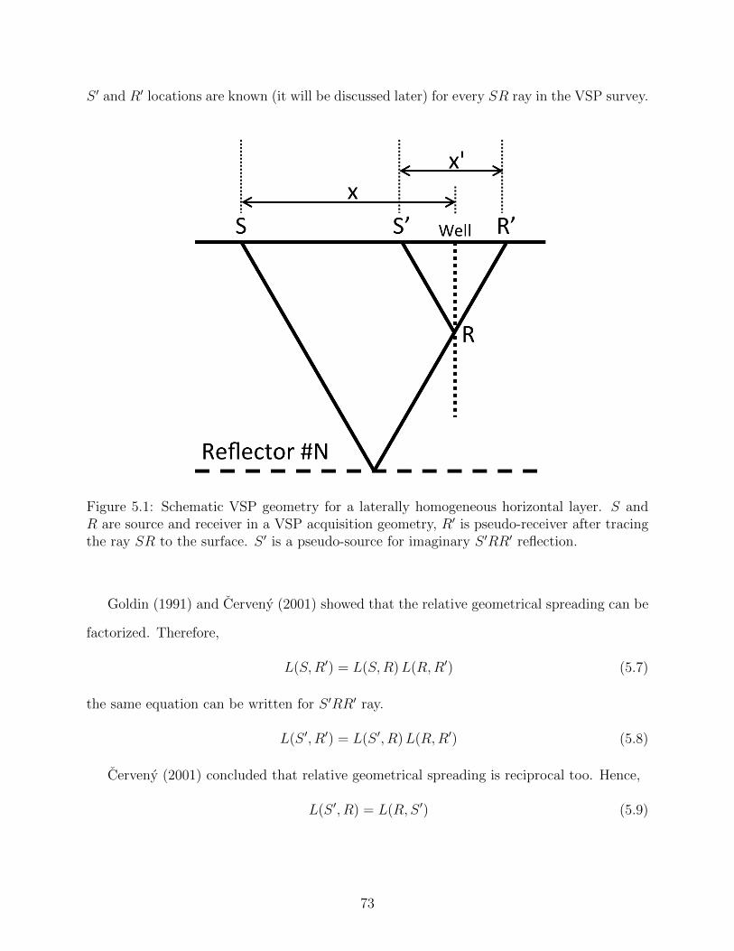
S ′ and R′ locations are known (it will be discussed later) for every SR ray in the VSP survey.

Figure 5.1: Schematic VSP geometry for a laterally homogeneous horizontal layer. S andR are source and receiver in a VSP acquisition geometry, R′ is pseudo-receiver after tracingthe ray SR to the surface. S ′ is a pseudo-source for imaginary S ′RR′ reflection.

Goldin (1991) and Cerveny (2001) showed that the relative geometrical spreading can be

factorized. Therefore,

L(S,R′) = L(S,R)L(R,R′) (5.7)

the same equation can be written for S ′RR′ ray.

L(S ′, R′) = L(S ′, R)L(R,R′) (5.8)

Cerveny (2001) concluded that relative geometrical spreading is reciprocal too. Hence,

L(S ′, R) = L(R, S ′) (5.9)

73

By substituting equation 5.9 into equation 5.8, we have

L(S ′, R′) = L(R, S ′)L(R,R′) (5.10)

Because of lateral homogeneity assumption and consequently symmetrical location of S ′

and R′ respect to R, one can can write

L(R, S ′) = L(R,R′). (5.11)

Therefore,

L(S ′, R′) = [L(R,R′)]2,

L(R,R′) =√L(S ′, R′).

(5.12)

Substituting equation (5.12) into equation (5.7) implies

L(S,R) =L(S,R′)√L(S ′, R′)

. (5.13)

Obviously, the main challenge for using equation 5.13 practically is to find R′ on the

earth surface (S ′ is the symmetric location of R′ respect to R). To find R′ for a VSP source-

receiver pair, we need velocity information above the target reflector in the borehole and

performing ray tracing. Note the ray tracing in this approach is not required for amplitude

correction, unlike dynamic ray tracing method. Anisotropic velocity model can be derived

from VSP data directly using techniques like the slowness-polarization method (de Parscau,

1991; de Parscau and Nicoletis, 1990; Dewangan and Grechka, 2003; Grechka and Mateeva,

2007; Horne and Leaney, 2000; Hsu et al., 1991; Tamimi and Davis, 2014).

Once the location of the pseudo-receiver R′ (and corresponding pseudo-source S ′) is

found, the offset between the pseudo-source S ′ and the pseudo-receiver R′ , called x′, and

the offset between source S and the pseudo-receiver R′, which is x+ 12x′, can be calculated.

For multiple reflectors and receivers, L(S,R), L(S,R′) and L(S ′, R′) can be rewritten as

L(S,R)⇒ L(N,R)(x),

L(S,R′)⇒ L(N)(x+1

2x′),

L(S ′, R′)⇒ L(R)(x′),

(5.14)

74

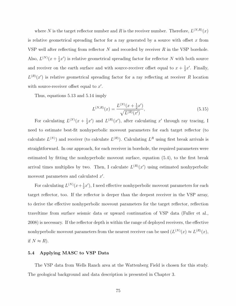
where N is the target reflector number and R is the receiver number. Therefore, L(N,R)(x)

is relative geometrical spreading factor for a ray generated by a source with offset x from

VSP well after reflecting from reflector N and recorded by receiver R in the VSP borehole.

Also, L(N)(x+ 12x′) is relative geometrical spreading factor for reflector N with both source

and receiver on the earth surface and with source-receiver offset equal to x + 12x′. Finally,

L(R)(x′) is relative geometrical spreading factor for a ray reflecting at receiver R location

with source-receiver offset equal to x′.

Thus, equations 5.13 and 5.14 imply

L(N,R)(x) =L(N)(x+ 1

2x′)√

L(R)(x′), (5.15)

For calculating L(N)(x + 12x′) and L(R)(x′), after calculating x′ through ray tracing, I

need to estimate best-fit nonhyperbolic moveout parameters for each target reflector (to

calculate L(N)) and receiver (to calculate L(R)). Calculating LR using first break arrivals is

straightforward. In our approach, for each receiver in borehole, the required parameters were

estimated by fitting the nonhyperbolic moveout surface, equation (5.4), to the first break

arrival times multiplies by two. Then, I calculate L(R)(x′) using estimated nonhyperbolic

moveout parameters and calculated x′.

For calculating L(N)(x+ 12x′), I need effective nonhyperbolic moveout parameters for each

target reflector, too. If the reflector is deeper than the deepest receiver in the VSP array,

to derive the effective nonhyperbolic moveout parameters for the target reflector, reflection

traveltime from surface seismic data or upward continuation of VSP data (Fuller et al.,

2008) is necessary. If the reflector depth is within the range of deployed receivers, the effective

nonhyperbolic moveout parameters from the nearest receiver can be used (L(N)(x) ≈ L(R)(x),

if N ≈ R).

5.4 Applying MASC to VSP Data

The VSP data from Wells Ranch area at the Wattenberg Field is chosen for this study.

The geological background and data description is presented in Chapter 3.

75

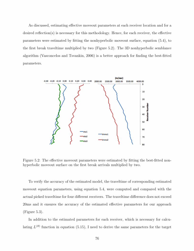
As discussed, estimating effective moveout parameters at each receiver location and for a

desired reflection(s) is necessary for this methodology. Hence, for each receiver, the effective

parameters were estimated by fitting the nonhyperbolic moveout surface, equation (5.4), to

the first break traveltime multiplied by two (Figure 5.2). The 3D nonhyperbolic semblance

algorithm (Vasconcelos and Tsvankin, 2006) is a better approach for finding the best-fitted

parameters.

Figure 5.2: The effective moveout parameters were estimated by fitting the best-fitted non-hyperbolic moveout surface on the first break arrivals multiplied by two.

To verify the accuracy of the estimated model, the traveltime of corresponding estimated

moveout equation parameters, using equation 5.4, were computed and compared with the

actual picked traveltime for four different receivers. The traveltime difference does not exceed

20ms and it ensures the accuracy of the estimated effective parameters for our approach

(Figure 5.3).

In addition to the estimated parameters for each receiver, which is necessary for calcu-

lating L(R) function in equation (5.15), I need to derive the same parameters for the target

76

Figure 5.3: Traveltime difference maps, ∆T = Tdata − Tmodel, where estimated traveltimefrom effective moveout parameters is Tmodel), and the actual traveltime is Tdata.

reflection and evaluate L(N) function too. Here, the target horizon, for correcting the geo-

metrical spreading, is top of the Niobrara Formation. Because the last receiver is only 39.7

m above the top of the Niobrara Formation, I used the effective moveout parameters from

the last receiver for this reflector.

The next step is to find the pseudo-receiver R′ and corresponding offset (x′) at the

surface for each source and receiver pair in the VSP survey. I used the ray tracing code

ANRAY (Gajewski and Psencık, 1990), to find pseudo-receiver locations. For performing

ray tracing, we need an anisotropic velocity model above the target horizon to trace the ray

back to the surface and find the pseudo-receiver location. In Chapter 3, I showed that NE

and SE lines are the vertical symmetry planes, and using joint P- and SV-wave slowness-

polarization method, a local anisotropic velocity model at the location of the VSP well is

built (Figure 5.4). Although the velocity model is 1D and local, there is no sign of significant

lateral heterogeneity in the VSP area, allowing us to extend the anisotropic velocity model

77

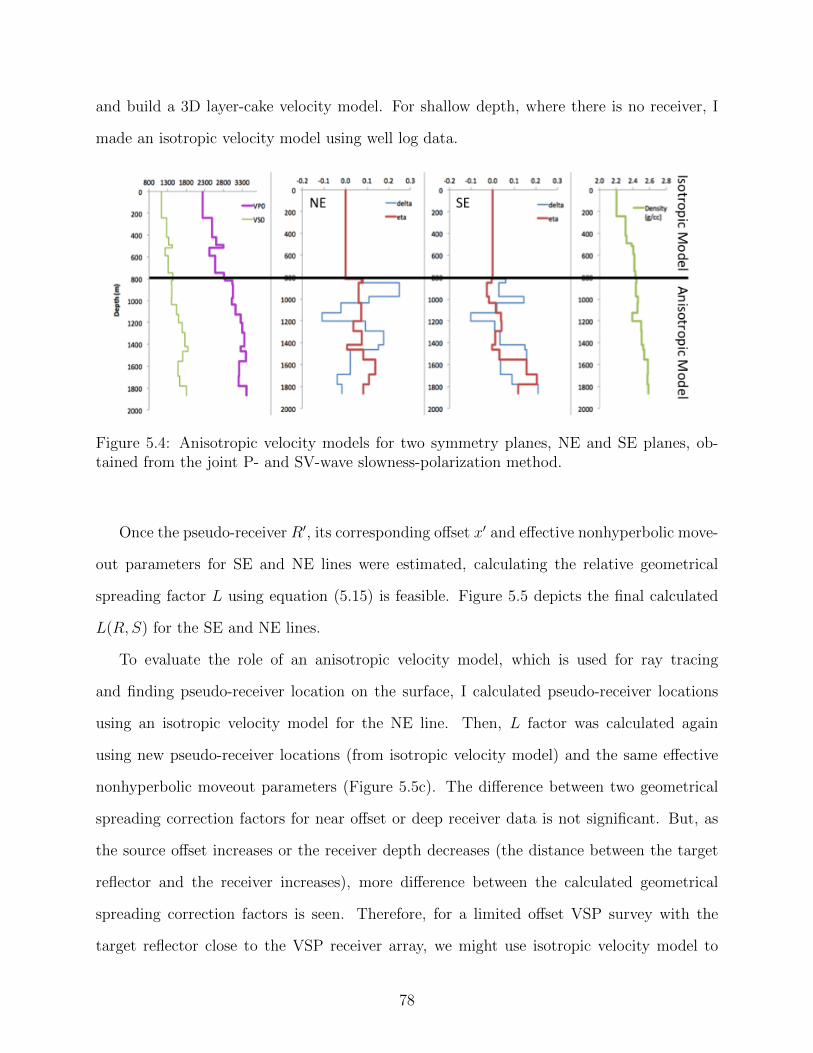
and build a 3D layer-cake velocity model. For shallow depth, where there is no receiver, I

made an isotropic velocity model using well log data.

Figure 5.4: Anisotropic velocity models for two symmetry planes, NE and SE planes, ob-tained from the joint P- and SV-wave slowness-polarization method.

Once the pseudo-receiver R′, its corresponding offset x′ and effective nonhyperbolic move-

out parameters for SE and NE lines were estimated, calculating the relative geometrical

spreading factor L using equation (5.15) is feasible. Figure 5.5 depicts the final calculated

L(R, S) for the SE and NE lines.

To evaluate the role of an anisotropic velocity model, which is used for ray tracing

and finding pseudo-receiver location on the surface, I calculated pseudo-receiver locations

using an isotropic velocity model for the NE line. Then, L factor was calculated again

using new pseudo-receiver locations (from isotropic velocity model) and the same effective

nonhyperbolic moveout parameters (Figure 5.5c). The difference between two geometrical

spreading correction factors for near offset or deep receiver data is not significant. But, as

the source offset increases or the receiver depth decreases (the distance between the target

reflector and the receiver increases), more difference between the calculated geometrical

spreading correction factors is seen. Therefore, for a limited offset VSP survey with the

target reflector close to the VSP receiver array, we might use isotropic velocity model to

78

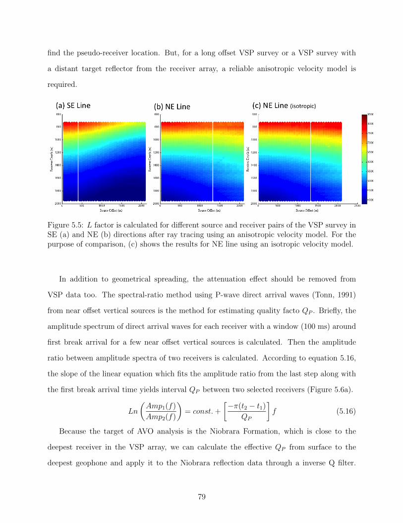
find the pseudo-receiver location. But, for a long offset VSP survey or a VSP survey with

a distant target reflector from the receiver array, a reliable anisotropic velocity model is

required.

Figure 5.5: L factor is calculated for different source and receiver pairs of the VSP survey inSE (a) and NE (b) directions after ray tracing using an anisotropic velocity model. For thepurpose of comparison, (c) shows the results for NE line using an isotropic velocity model.

In addition to geometrical spreading, the attenuation effect should be removed from

VSP data too. The spectral-ratio method using P-wave direct arrival waves (Tonn, 1991)

from near offset vertical sources is the method for estimating quality facto QP . Briefly, the

amplitude spectrum of direct arrival waves for each receiver with a window (100 ms) around

first break arrival for a few near offset vertical sources is calculated. Then the amplitude

ratio between amplitude spectra of two receivers is calculated. According to equation 5.16,

the slope of the linear equation which fits the amplitude ratio from the last step along with

the first break arrival time yields interval QP between two selected receivers (Figure 5.6a).

Ln

(Amp1(f)

Amp2(f)

)= const.+

[−π(t2 − t1)

QP

]f (5.16)

Because the target of AVO analysis is the Niobrara Formation, which is close to the

deepest receiver in the VSP array, we can calculate the effective QP from surface to the

deepest geophone and apply it to the Niobrara reflection data through a inverse Q filter.

79

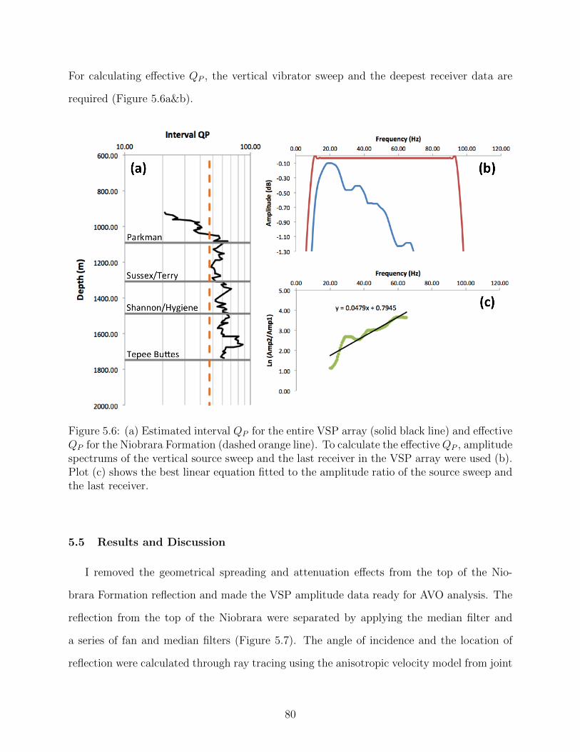
For calculating effective QP , the vertical vibrator sweep and the deepest receiver data are

required (Figure 5.6a&b).

Figure 5.6: (a) Estimated interval QP for the entire VSP array (solid black line) and effectiveQP for the Niobrara Formation (dashed orange line). To calculate the effectiveQP , amplitudespectrums of the vertical source sweep and the last receiver in the VSP array were used (b).Plot (c) shows the best linear equation fitted to the amplitude ratio of the source sweep andthe last receiver.


I removed the geometrical spreading and attenuation effects from the top of the Nio-

brara Formation reflection and made the VSP amplitude data ready for AVO analysis. The

reflection from the top of the Niobrara were separated by applying the median filter and

a series of fan and median filters (Figure 5.7). The angle of incidence and the location of

reflection were calculated through ray tracing using the anisotropic velocity model from joint

80

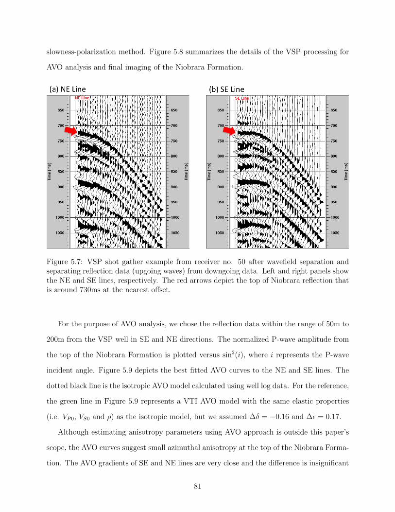
slowness-polarization method. Figure 5.8 summarizes the details of the VSP processing for

AVO analysis and final imaging of the Niobrara Formation.

Figure 5.7: VSP shot gather example from receiver no. 50 after wavefield separation andseparating reflection data (upgoing waves) from downgoing data. Left and right panels showthe NE and SE lines, respectively. The red arrows depict the top of Niobrara reflection thatis around 730ms at the nearest offset.

For the purpose of AVO analysis, we chose the reflection data within the range of 50m to

200m from the VSP well in SE and NE directions. The normalized P-wave amplitude from

the top of the Niobrara Formation is plotted versus sin2(i), where i represents the P-wave

incident angle. Figure 5.9 depicts the best fitted AVO curves to the NE and SE lines. The

dotted black line is the isotropic AVO model calculated using well log data. For the reference,

the green line in Figure 5.9 represents a VTI AVO model with the same elastic properties

(i.e. VP0, VS0 and ρ) as the isotropic model, but we assumed ∆δ = −0.16 and ∆ε = 0.17.

Although estimating anisotropy parameters using AVO approach is outside this paper’s

scope, the AVO curves suggest small azimuthal anisotropy at the top of the Niobrara Forma-

tion. The AVO gradients of SE and NE lines are very close and the difference is insignificant

81

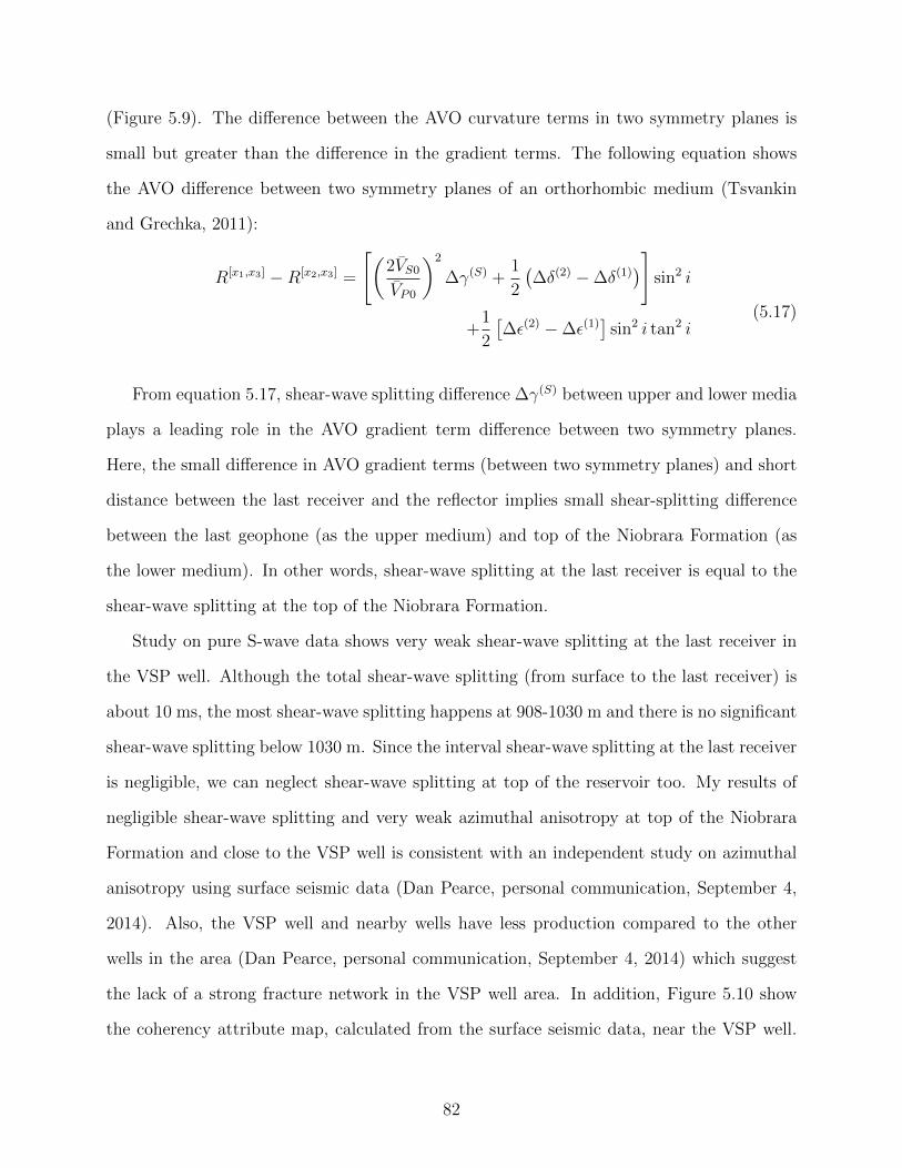
(Figure 5.9). The difference between the AVO curvature terms in two symmetry planes is

small but greater than the difference in the gradient terms. The following equation shows

the AVO difference between two symmetry planes of an orthorhombic medium (Tsvankin

and Grechka, 2011):

R[x1,x3] −R[x2,x3] =

[(2VS0VP0

)2

∆γ(S) +1

2

(∆δ(2) −∆δ(1)

)]sin2 i

+1

2

[∆ε(2) −∆ε(1)

]sin2 i tan2 i

(5.17)

From equation 5.17, shear-wave splitting difference ∆γ(S) between upper and lower media

plays a leading role in the AVO gradient term difference between two symmetry planes.

Here, the small difference in AVO gradient terms (between two symmetry planes) and short

distance between the last receiver and the reflector implies small shear-splitting difference

between the last geophone (as the upper medium) and top of the Niobrara Formation (as

the lower medium). In other words, shear-wave splitting at the last receiver is equal to the

shear-wave splitting at the top of the Niobrara Formation.

Study on pure S-wave data shows very weak shear-wave splitting at the last receiver in

the VSP well. Although the total shear-wave splitting (from surface to the last receiver) is

about 10 ms, the most shear-wave splitting happens at 908-1030 m and there is no significant

shear-wave splitting below 1030 m. Since the interval shear-wave splitting at the last receiver

is negligible, we can neglect shear-wave splitting at top of the reservoir too. My results of

negligible shear-wave splitting and very weak azimuthal anisotropy at top of the Niobrara

Formation and close to the VSP well is consistent with an independent study on azimuthal

anisotropy using surface seismic data (Dan Pearce, personal communication, September 4,

2014). Also, the VSP well and nearby wells have less production compared to the other

wells in the area (Dan Pearce, personal communication, September 4, 2014) which suggest

the lack of a strong fracture network in the VSP well area. In addition, Figure 5.10 show

the coherency attribute map, calculated from the surface seismic data, near the VSP well.

82

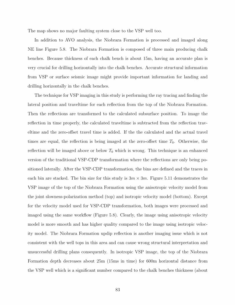
The map shows no major faulting system close to the VSP well too.

In addition to AVO analysis, the Niobrara Formation is processed and imaged along

NE line Figure 5.8. The Niobrara Formation is composed of three main producing chalk

benches. Because thickness of each chalk bench is about 15m, having an accurate plan is

very crucial for drilling horizontally into the chalk benches. Accurate structural information

from VSP or surface seismic image might provide important information for landing and

drilling horizontally in the chalk benches.

The technique for VSP imaging in this study is performing the ray tracing and finding the

lateral position and traveltime for each reflection from the top of the Niobrara Formation.

Then the reflections are transformed to the calculated subsurface position. To image the

reflection in time properly, the calculated traveltime is subtracted from the reflection trav-

eltime and the zero-offset travel time is added. If the the calculated and the actual travel

times are equal, the reflection is being imaged at the zero-offset time T0. Otherwise, the

reflection will be imaged above or below T0 which is wrong. This technique is an enhanced

version of the traditional VSP-CDP transformation where the reflections are only being po-

sitioned laterally. After the VSP-CDP transformation, the bins are defined and the traces in

each bin are stacked. The bin size for this study is 3m× 3m. Figure 5.11 demonstrates the

VSP image of the top of the Niobrara Formation using the anisotropic velocity model from

the joint slowness-polarization method (top) and isotropic velocity model (bottom). Except

for the velocity model used for VSP-CDP transformation, both images were processed and

imaged using the same workflow (Figure 5.8). Clearly, the image using anisotropic velocity

model is more smooth and has higher quality compared to the image using isotropic veloc-

ity model. The Niobrara Formation updip reflection is another imaging issue which is not

consistent with the well tops in this area and can cause wrong structural interpretation and

unsuccessful drilling plans consequently. In isotropic VSP image, the top of the Niobrara

Formation depth decreases about 25m (15ms in time) for 600m horizontal distance from

the VSP well which is a significant number compared to the chalk benches thickness (about

83

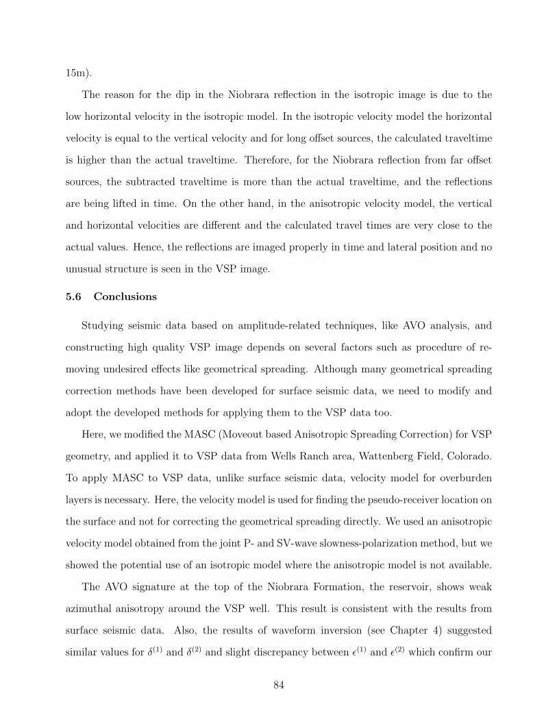
15m).

The reason for the dip in the Niobrara reflection in the isotropic image is due to the

low horizontal velocity in the isotropic model. In the isotropic velocity model the horizontal

velocity is equal to the vertical velocity and for long offset sources, the calculated traveltime

is higher than the actual traveltime. Therefore, for the Niobrara reflection from far offset

sources, the subtracted traveltime is more than the actual traveltime, and the reflections

are being lifted in time. On the other hand, in the anisotropic velocity model, the vertical

and horizontal velocities are different and the calculated travel times are very close to the

actual values. Hence, the reflections are imaged properly in time and lateral position and no

unusual structure is seen in the VSP image.

5.6 Conclusions

Studying seismic data based on amplitude-related techniques, like AVO analysis, and

constructing high quality VSP image depends on several factors such as procedure of re-

moving undesired effects like geometrical spreading. Although many geometrical spreading

correction methods have been developed for surface seismic data, we need to modify and

adopt the developed methods for applying them to the VSP data too.

Here, we modified the MASC (Moveout based Anisotropic Spreading Correction) for VSP

geometry, and applied it to VSP data from Wells Ranch area, Wattenberg Field, Colorado.

To apply MASC to VSP data, unlike surface seismic data, velocity model for overburden

layers is necessary. Here, the velocity model is used for finding the pseudo-receiver location on

the surface and not for correcting the geometrical spreading directly. We used an anisotropic

velocity model obtained from the joint P- and SV-wave slowness-polarization method, but we

showed the potential use of an isotropic model where the anisotropic model is not available.

The AVO signature at the top of the Niobrara Formation, the reservoir, shows weak

azimuthal anisotropy around the VSP well. This result is consistent with the results from

surface seismic data. Also, the results of waveform inversion (see Chapter 4) suggested

similar values for δ(1) and δ(2) and slight discrepancy between ε(1) and ε(2) which confirm our

84

azimuthal AVO observation. The weak azimuthal AVO response can imply lack of fracture

networks, which justifies the low hydrocarbon production for the wells in the VSP area.

Also, the final image, using anisotropic velocity model from the joint slowness polarization

method has improved significantly and shows the importance of anisotropy in the Niobrara

shale play.

85

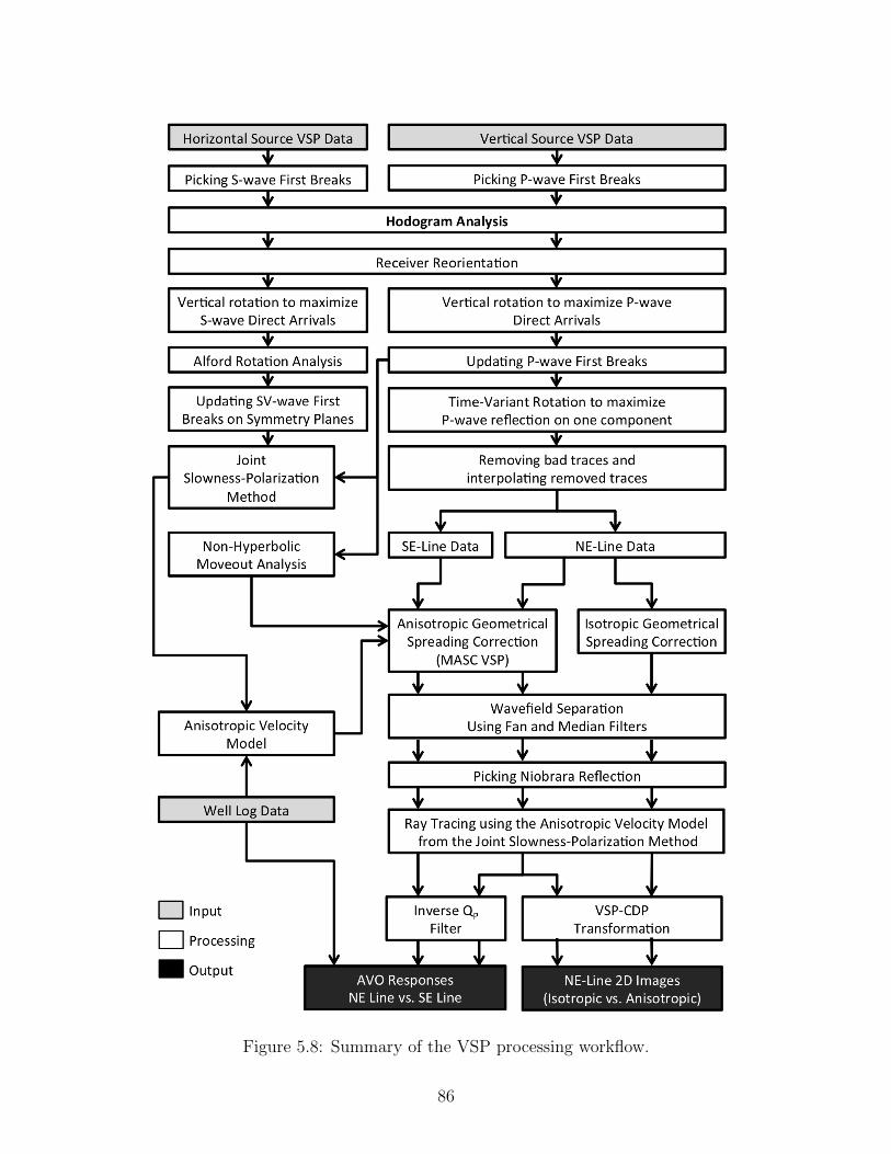
Figure 5.8: Summary of the VSP processing workflow.

86

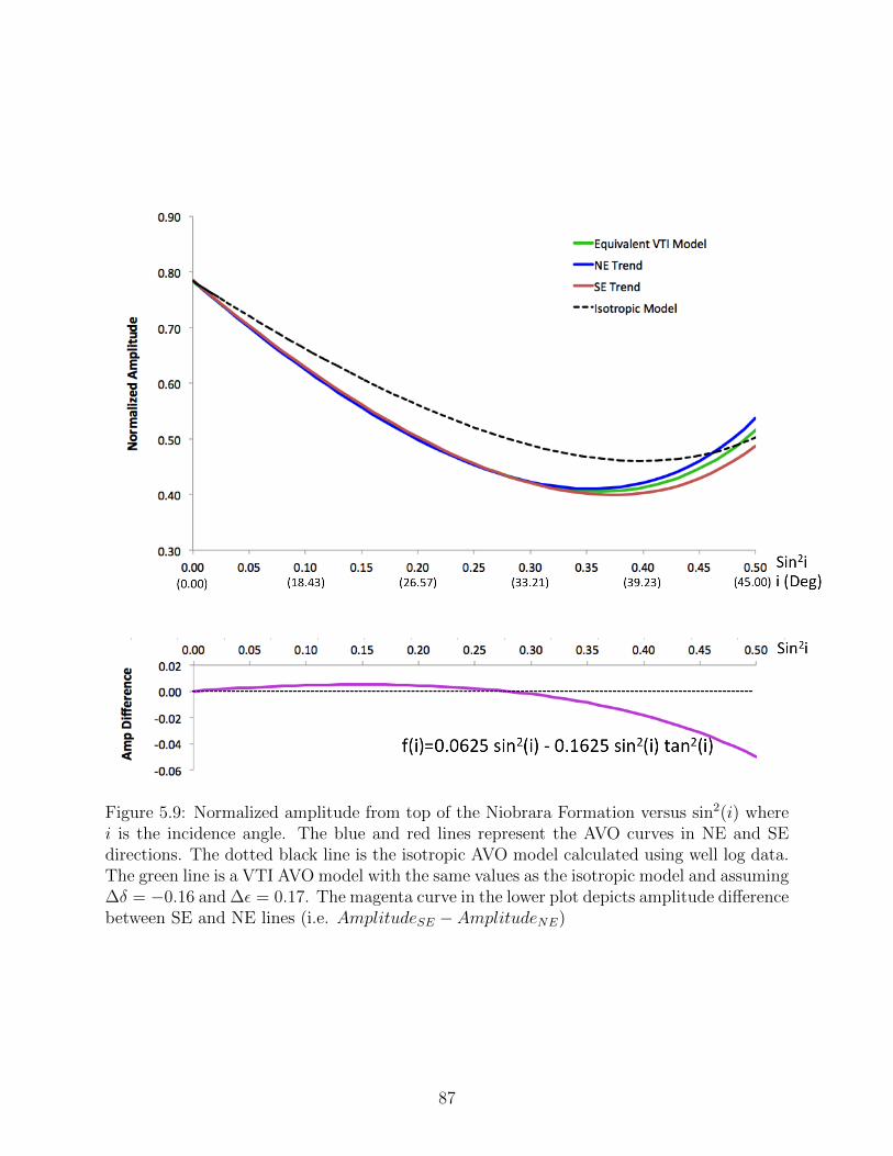
Figure 5.9: Normalized amplitude from top of the Niobrara Formation versus sin2(i) wherei is the incidence angle. The blue and red lines represent the AVO curves in NE and SEdirections. The dotted black line is the isotropic AVO model calculated using well log data.The green line is a VTI AVO model with the same values as the isotropic model and assuming∆δ = −0.16 and ∆ε = 0.17. The magenta curve in the lower plot depicts amplitude differencebetween SE and NE lines (i.e. AmplitudeSE − AmplitudeNE)

87

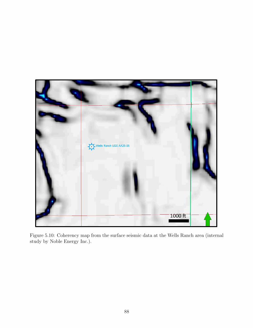
Figure 5.10: Coherency map from the surface seismic data at the Wells Ranch area (internalstudy by Noble Energy Inc.).

88

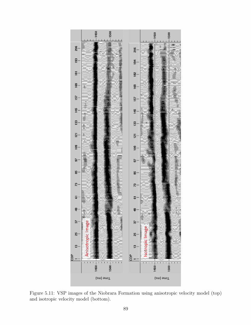
Figure 5.11: VSP images of the Niobrara Formation using anisotropic velocity model (top)and isotropic velocity model (bottom).

89

CHAPTER 6

CONCLUSIONS AND RECOMMENDATIONS

Ignoring anisotropy can lead to misleading information and imperfect seismic imag-

ing. On the other hand, taking anisotropy into account requires reliable parameter estima-

tion. I introduce the joint slowness-polarization method as a reliable method for extracting

anisotropy information from multicomponent VSP data. The anisotropic velocity model ob-

tained from the joint slowness-polarization method were used for more accurate azimuthal

AVO analysis and final VSP imaging. The main conclusions and recommendations for this

research are summarized:

6.1 Conclusions

The following conclusions are drawn:

• The joint P- and SV-wave slowness-polarization method improved seismic imaging of

a multicomponent VSP data set in the Wattenberg Field, Colorado.

• In testing the joint slowness-polarization method with a combination of P-wave and

converted SV-wave data, the estimation error is larger than that for the joint P- and

pure SV-wave slowness-polarization method.

• Applying the joint P- and pure SV-wave slowness-polarization method to a 9C VSP

dataset from Wattenberg Field confirms that the technique can be applied to any

multicomponent VSP datasets with high-quality P- and SV-waves.

• Elastic parameters are determined by analyzing prestack AVO and imaging the VSP

data from the Niobrara Formation. The result of azimuthal AVO analysis on top of the

Niobrara Formation shows weak azimuthal anisotropy near the VSP well. The main

90

reason for weak azimuthal anisotropy at top of the Niobrara Formation is the lack of

open natural fractures near the well location.

• Two 2D VSP images of the Niobrara Formation using anisotropic and isotropic velocity

models were constructed. Unlike the isotropic image, the anisotropic image is flat

and the top of Niobrara Formation depth does not change significantly. Hence, the

isotropic image can mislead horizontal drilling program in this area and reduce the

contact between the drilled well and chalk benches which have thicknesses of about

15m.

6.2 Recommendations

My main recommendations for future research on the thesis topic are:

• I used a weighted sum method for defining the objective function for the joint slowness-

polarization method. This approach is is generally biased by the choice of the individual

weights. In Chapter 3, the NSGA II, as an optimization approach, is explained for the

waveform inversion. I believe this approach can be applied to the joint slowness-

polarization method and yield more reliable results.

• For an unbiased comparison, no information from the slowness-polarization method is

used for the waveform inversion. But the slowness-polarization method can provide a

good initial model for the waveform inversion process. Since the computational time is

one of the challenges for the waveform inversion, a study on building an initial model

for the waveform inversion using the slowness-polarization method is recommended.

• The last recommendation for future research is utilizing miscroseismic data in the

joint slowness-polarization method. In general, for the slowness-polarization method,

we need the vertical slowness and polarization angle. Both types of the data can be

calculated from good quality microseismic data using 3C geophones in a vertical well.

In the case of P- and S-wave microseismic arrivals, the joint slowness-polarization

91

method can be used to characterize the anisotropy around the VSP receiver array.

However, separating SV-wave and SH-wave arrivals is crucial and needs special efforts.

Also, monitor wells should be close to the treatment well, to record good quality data

and various range of polarization angle.

92

REFERENCES CITED

Al-Dajani, A., I. Tsvankin, and M. Toksoz, 1998, Non-hyperbolic reflection moveout forazimuthally anisotropic media: 68th SEG Annual Meeting, SEG Technical Program Ex-panded Abstract, 1479–1482.

Alkhalifah, T., and I. Tsvankin, 1995, Velocity analysis of transversely isotropic media:Geophysics, 60, 1550–1566.

Backus, G. E., 1965, Possible form of seismic anisotropy of the upper most mantle underocean: Journal of Geophysical Research, 70, 3429–3439.

Bayuk, I. O., M. Ammerman, and E. M. Chesnokov, 2007, Elastic moduli of anisotropicclay: Geophysics, 72, D107–D117.

Brittan, J., J. Bai, H. Delome, C. Wang, and D. Yingst, 2013, Full waveform inversion - thestate of the art: First Break, 31, 75–81.

Crampin, S., 1978, Seismic wave propagation through a cracked solid: Polarization as apossible dilatancy diagnostic: Geophysical Journal of the Royal Astronomical Society, 53,467–496.

——–, 1981, A review of wave motion in a anisotropic and cracked elastic media: WaveMotion, 3, 343–391.

——–, 1983, Shear-wave polarizations: A plea for three-component recording: Presented atthe 53rd SEG Annual Meeting, SEG Technical Program Expanded Abstract.

——–, 1987, Shear-wave polarizations: A plea for three-component recording, in S. Danbomand N. Domenico, eds., Shear-wave exploration: SEG, Geophysical Developments 1, 227–251.

Davis, T. L., 2005, Seismic monitoring of a fractured reservoir, Weyburn Field, Saskatchewan:The Mountain Geologist, 42, 45–52.

de Parscau, J., 1991, Relationship between phase velocities and polarization in transverselyisotopic media: Geophysics, 56, 1578–1583.

de Parscau, J., and L. Nicoletis, 1990, Tranverse isotropy estimation from multioffset VSPs:60th SEG Annual Meeting, SEG Technical Program Expanded Abstract, 1439–1442.

93

Deb, K., A. Pratap, S. Agrawal, and T. Meyarivan, 2002, A fast and elitist multiobjectivegenetic algorithm: NSGA-II: IEEE Transactions on Evolutionary Computation, 6, 182–197.

DeVault, B., T. L. Davis, I. Tsvankin, R. Verm, and F. Hilterman, 2002, MulticomponentAVO analysis, Vacuum Field, New Mexico: Geophysics, 67, 701–710.

Dewangan, P., and V. Grechka, 2003, Inversion of multicomponent, multiazimuthal, walka-way VSP data for stiffness tensor: Geophysics, 68, 1022–1031.

Farra, V., 2001, Higher-order perturbation of the phase velocity and polarization of qP andqS waves in anisotropic media: Geophysical Journal International, 147, 93–104.

Fuller, B. N., M. Sterling, and R. Van Dok, 2008, Time domain 2D VSP and 3D VSP pro-cessing: Presented at the 78th SEG Annual Meeting, SEG Technical Program ExpandedAbstract.

Gaiser, J. E., 1990, Transversely isotropic phase velocity analysis from slowness estimates:Journal of Geophysical Research, 95, 11241–11254.

Gajewski, D., and I. Psencık, 1990, Vertical seismic profile synthetics by dynamic ray tracingin laterally varying layered anisotropic structure: Journal of Geophysical Research, 95,11301–11315.

Goldberg, D. E., 1989, Genetic algorithms in search, optimization and machine learning:Addison-Wesley Longman Publishing Co., Inc.

Goldin, S. V., 1991, Decomposition of geometrical approximation of a reflected wave: Geol-ogy and Geophysics, 32, 128–137.

Grechka, V., P. Jorgensen, and L. Lopez, 2006, Anisotropy estimation from marine 3D VSPdata: Offshore Technology Conference, OTC17866.

Grechka, V., and A. Mateeva, 2007, Inversion of P-wave VSP data for local anisotropy:Theory and case study: Geophysics, 72, D69–79.

Grechka, V., A. Mateeva, C. Gentry, P. Jorgensen, and J. Lopez, 2007, Estimation of seismicanisotropy from P-wave VSP data: The Leading Edge, 26, 756–759.

Gupta, I. N., 1973a, Dilatancy and premonitory variations of P, S travel times: Bulletin ofthe Seismological Society of America, 63, 1157–1161.

——–, 1973b, Premonitory variations in S-wave velocity anisotropy before earthquakes inNevada: Science, 182, 1129–1132.

94

Hardage, B. A., M. V. DeAngelo, P. E. Murray, and D. Sava, 2011, Multicomponent seismictechnology: Society of Exploration Geophysicists. Geophysical References Series, No. 18.

Heidbach, O., M. Tingay, A. Barth, J. Reinecker, K. Kurfeß, and B. Muller, 2008, The worldstress map database release 2008: Technical Report GFZ.WSM.Rel2008.

Helbig, K., and L. Thomsen, 2005, 75-plus years of anisotropy in exploration and reservoirseismics: A historical review of concepts and methods: Geophysics, 70, 9ND–23ND.

Higley, D. K., D. O. Cox, and R. J. Weimer, 2003, Petroleum system and production char-acteristics of the muddy J sandstone (Lower Cretaceous) Wattenberg continous gas Field,Denver Basin, Colorado: AAPG Bulletin, 87, 15–37.

Hornby, B. E., L. M. Schwartzt, and J. A. Hudson, 1994, Anisotropic effective-mediummodeling of the elastic properties of shales: Geophysics, 59, 1570–1583.

Horne, S., and S. Leaney, 2000, Short note: Polarization and slowness component inversionfor TI anisotropy: Geophysical Prospecting, 48, 779–788.

Hsu, K., M. Schoenberg, and J. Walsh, 1991, Anisotropy from polarization and moveout:A case study: 61st SEG Annual Meeting, SEG Technical Program Expanded Abstract,1526–1529.

Jılek, P., B. Hornby, and A. Ray, 2003, Inversion of 3D VSP P-wave data for local anisotropy:A case study: 73rd SEG Annual Meeting, SEG Technical Program Expanded Abstract,1322–1325.

Kaiser, C. A., and S. A. Sonnenberg, 2013, The Graneros-Greenhorn petroleum system:Greater Wattenberg area, Denver basin, Colorado.: The Mountain Geologist, 51, 35–81.

Kamath, N., and I. Tsvankin, 2013, Full-waveform inversion of multicomponent data forhorizontally layered VTI media: Geophysics, 78, WC113–WC121.

Li, T., and S. Mallick, 2013, Prestack waveform inversion of four-component, two-azimuthsurface seismic data for orthorhombic elastic media parameters using a nondominatedsorting genetic algorithm: Presented at the 83rd SEG Annual Meeting, SEG TechnicalProgram Expanded Abstract.

——–, 2014a, Multicomponent, multiazimuth prestack seismic waveform inversion for az-imuthally anisotropic media using a parallel and computationally efficient nondominatedsorting genetic algorithm. Submitted to Geophysical Prospecting.

95

——–, 2014b, Prestack waveform inversion of three-component, two-azimuth surface seismicdata for azimuthally dependent anisotropic parameters using a parallelized nondominatedsorting genetic algorithm: Presented at the 84th SEG Annual Meeting, SEG TechnicalProgram Expanded Abstract.

MacBeth, C., 1991, Inverting shear-wave polarization for anisotropy using three-componentoffset VSPs: Synthetic seismogram: Geophysical Journal International, 107, 571–583.

Mallick, S., K. Craft, L. Meister, and R. Chambers, 1998, Determination of the principaldirections of azimuthal anisotropy from P-wave seismic data: Geophysics, 63, 692–708.

Marron, J. S., and A. B. Tsybakov, 1995, Visual error criteria for qualitative smoothing:Journal of the American Statistical Association, 90, 499–507.

Martinez, R. D., 1993, Wave propagation effects on amplitude variation with offset measure-ments: A modeling study: Geophysics, 58, 534–543.

Maultzsch, S., S. Horne, S. Archer, and H. Burkhardt, 2003, Effects of an anisotropic overbur-den on azimuthal amplitude analysis in horizontal transverse isotropic media: Geophysics,51, 61–74.

Miller, D. E., and C. Spencer, 1994, An exact inversion for anisotropic moduli from phaseslowness data: Journal of Geophysical Research, 99, 21651–21657.

Minas, C., S. J. Waddell, and G. Montana, 2011, Distance-based differential analysis of genecurves: Bioinformatics, 27, 3135–3141.

Padhi, A., and S. Mallick, 2013, Accurate estimation of density from the inversion of mul-ticomponent prestack seismic waveform data using a nondominated sorting genetic algo-rithm: The Leading Edge, 32, 94–98.

Pech, A., and I. Tsvankin, 2004, Quartic moveout coefficient for a dipping azimuthallyanisotropic layer: Geophysics, 69, 699–707.

Pevzner, R., B. Guervich, and M. Urosevic, 2011, Estimation of azimuthal anisotropy fromVSP data using multicomponent S-wave velocity analysis: Geophysics, 76, D1–D9.

Psencık, I., and D. Gajewski, 1998, Polarization, phase velocity, and NMO velocity of qP-waves in arbitrary weakly anisotropic media: Geophysics, 63, 1754–1766.

Ramos, A. C., and T. L. Davis, 1997, 3-D AVO analysis and modeling applited to fracturedetection in coalbed methane reservoirs: Geophysics, 62, 1683–1695.

Reshetnikov, A., 2013, Microseismic reflection imaging: Master’s thesis, Freie UniversitatBerlin.

96

Rusmanugroho, H., and G. A. McMechan, 2012a, 3D 9C seismic modeling and inversion ofWeyburn field data: Geophysics, 77, R161–R173.

——–, 2012b, Sensitivity of estimated elastic moduli to completeness of wave type, mea-surement type, and illumination aperture at a receiver in multicomponent VSP data:Geophysics, 77, R1–R18.

Samson, J. C., 1977, Matrix and stokes vector representations of detectors for polarizedwaveforms: theory, with some applications to teleseismic waves: Geophysical Journal ofthe Royal Astronomical Society, 51, 583–603.

Singh, P., and T. L. Davis, 2011, Advantages of shear wave seismic in Morrow sandstonedetection: International Journal of Geophysics, 2011, 1–16.

Tamimi, N., and T. L. Davis, 2012, Imaging the Morrow A sandstone using shear wave VSPdata, Postle Field, Oklahoma: International Journal of Geophysics, 2012, 1–14.

——–, 2014, Using P- and SV-wave VSP data for estimating local seismic anisotropy param-eters in VTI media with lateral heterogeneity in the overburden: Presented at the 84thSEG Annual Meeting, SEG Technical Program Expanded Abstract.

Tamimi, N., and P. Singh, 2012, Analysis of different well log and seismic data for estimatingshear wave polarization direction: Presented at the 82nd SEG Annual Meeting, SEGTechnical Program Expanded Abstract.

Thomsen, L., 1986, Weak elastic anisotropy: Geophysics, 51, 1954–1966.

Tonn, R., 1991, The determination of seismic quality factor q from vsp data: A comparisonof different computational methods: Geophysical Prospecting, 39, 1–27.

Tsvankin, I., 1997, Anistropic parameters and P-wave velocity for orthorhombic media:Geophysics, 62, 1292–1309.

——–, 2001, Seismic signature and analysis of reflection data in anisotropic media: PergamonPress, Inc.

Tsvankin, I., and V. Grechka, 2011, Seismology of azimuthally anisotropic media and seis-mic fracture characterization: Society of Exploration Geophysicists. Geophysical Series,No. 17.

Tsvankin, I., and L. Thomsen, 1994, Non-hyperbolic reflection moveout in anisotropic media:Geophysics, 59, 1290–1304.

97

US Energy Information Administration, 2014, Drilling productivity report: Technical report,US Energy Information Administration.

Vasconcelos, I., and I. Tsvankin, 2006, Nonhyperbolic moveout inversion of wide-azimuthP-wave data for orthorhombic media: Geophysical Prospecting, 54, 535–552.

Cerveny, V., 2001, Seismic ray theory: Cambridge University Press.

Virieux, J., and S. Opetro, 2009, An overview of full-waveform inversion in explorationgeophysics: Geophysics, 74, WCC1–WCC26.

White, J. E., L. Martineau-Nicoletis, and C. Monash, 1983, Measured anisotropy in Pierreshale: Geophysical Prospecting, 31, 709–725.

Xu, X., and I. Tsvankin, 2006, Anisotropic geometrical-spreading correction for wide-azimuthP-wave reflections: Geophysics, 71, D161–D170.

Xu, X., I. Tsvankin, and A. Pech, 2005, Geometrical spreading of P-waves in horizontallylayered, azimuthally anisotropic media: Geophysics, 70, D43–D53.

98

APPENDIX - WEAK ANISOTROPY APPROXIMATION OF SV-WAVE VERTICAL

SLOWNESS AS A FUNCTION OF POLARIZATION ANGLE IN A VTI MEDIUM

For P-wave, Grechka and Mateeva (2007) showed that

ψP = θ + ψAniso. (A.1)

where,

ψAniso = f0(δ + 2η sin2 θ) sin θ cos θ =1

2f0 sin 2θ(δ + 2η sin2 θ). (A.2)

Now, if we define νSV as the angle between the SV-wave polarization angle and the

horizontal line in a VTI medium (Figure A.1),

νSV = ψP = θ + ψAniso.,

θ = νSV − ψAniso.(A.3)

Also, corresponding SV-wave velocity can be written as

VSV (θ) = VS0(1 + σ sin2 θ cos2 θ). (A.4)

Hence, the SV-wave vertical slowness is

pSV (θ) =1

VS0(1− σ sin2 θ cos2 θ). (A.5)

From equation A.5, the vertical slowness component of SV-wave is

p3,SV (θ) = qSV (θ) =cos(θ)

VS0(1− σ sin2 θ cos2 θ) ≈ cos(θ)

VS0(1− σ sin2 νSV cos2 νSV ). (A.6)

If we substitute equation A.1 into equation A.6

qSV = cos(νSV − ψAniso.)(1− σ sin2 νSV cos2 νSV )

VS0. (A.7)

Then, using ψAniso. from equation A.2, cos(νSV − ψAniso.) can be rewritten as

cos(νSV − ψAniso.) = cos νSV cosψAniso. + sin νSV sinψAniso. ≈ cos νSV + ψAniso. sin νSV .(A.8)

99

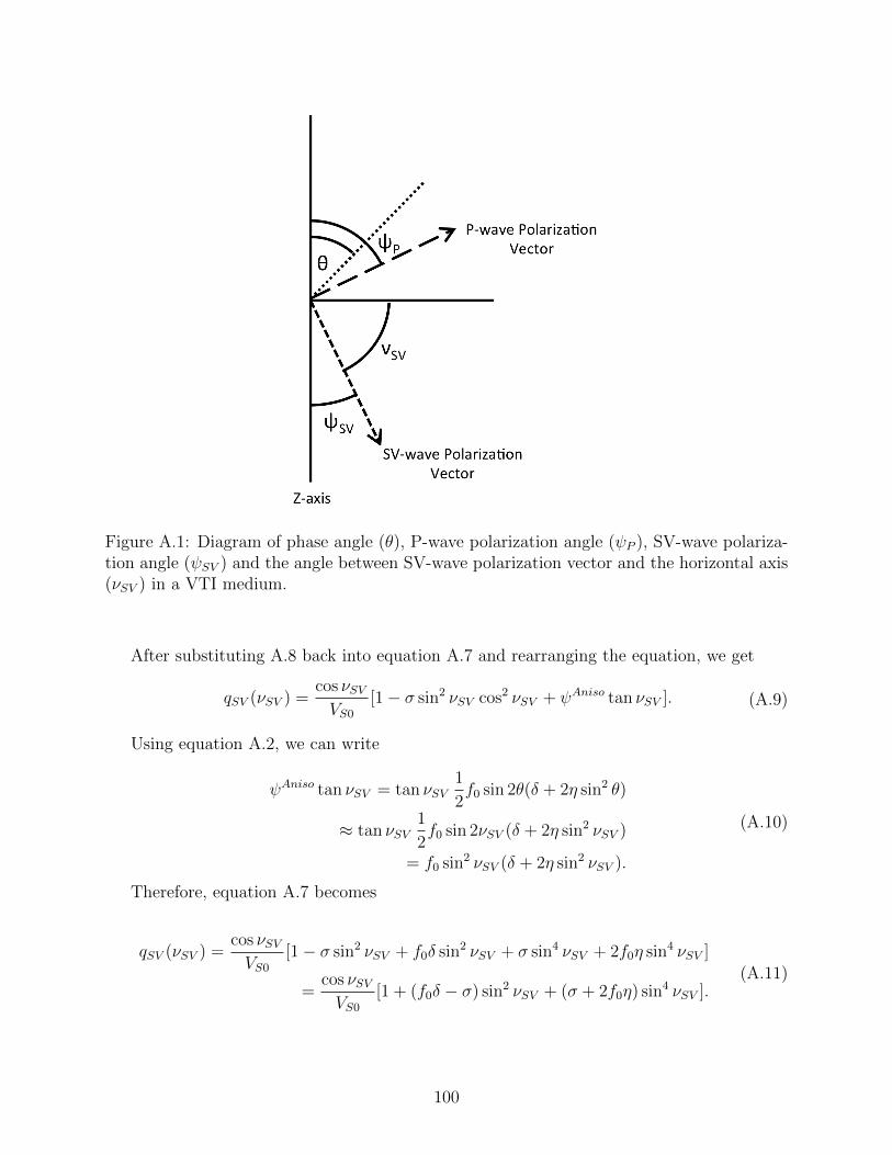
Figure A.1: Diagram of phase angle (θ), P-wave polarization angle (ψP ), SV-wave polariza-tion angle (ψSV ) and the angle between SV-wave polarization vector and the horizontal axis(νSV ) in a VTI medium.

After substituting A.8 back into equation A.7 and rearranging the equation, we get

qSV (νSV ) =cos νSVVS0

[1− σ sin2 νSV cos2 νSV + ψAniso tan νSV ]. (A.9)

Using equation A.2, we can write

ψAniso tan νSV = tan νSV1

2f0 sin 2θ(δ + 2η sin2 θ)

≈ tan νSV1

2f0 sin 2νSV (δ + 2η sin2 νSV )

= f0 sin2 νSV (δ + 2η sin2 νSV ).

(A.10)

Therefore, equation A.7 becomes

qSV (νSV ) =cos νSVVS0

[1− σ sin2 νSV + f0δ sin2 νSV + σ sin4 νSV + 2f0η sin4 νSV ]

=cos νSVVS0

[1 + (f0δ − σ) sin2 νSV + (σ + 2f0η) sin4 νSV ].(A.11)

100

As mentioned, νSV is the angle between the SV-wave polarization vector and the hori-

zontal axis Figure A.1. We usually calculate the polarization angle respect to the vertical

axis (we call it ψSV ). The equation A.11 in terms of ψSV , where ψSV = π2− νSV , is


[1 + (f0δ − σ) cos2 ψSV + (σ + 2f0η) cos4 ψSV ]. (A.12)

Also equation A.12 can be simplified by using:

δ + 2f0η = f0(σ + η),

f0δ − σ = f0(ε− σ).(A.13)

If we substitute equations A.13 into equation A.12,


[1 + f0(ε− σ) cos2 ψSV + f0(σ + η) cos4 ψSV ]. (A.14)

101

determination of seismic anisotropy parameters from

Documents