relationships between highway capacity and induced …sensibletransportation.org/pdf/noland.pdf ·...

Relationships between highway capacity and induced vehicletravel

Robert B. Noland *

University of London Centre for Transport Studies, Department of Civil and Environmental Engineering,

Imperial College of Science, Technology and Medicine, London SW7 2BU, UK

Received 4 March 1999; received in revised form 1 July 1999; accepted 6 July 1999

Abstract

The theory of induced travel demand asserts that increases in highway capacity will induce additionalgrowth in tra�c. This can occur through a variety of behavioral mechanisms including mode shifts, routeshifts, redistribution of trips, generation of new trips, and long run land use changes that create new tripsand longer trips. The objective of this paper is to statistically test whether this e�ect exists and to empiricallyderive elasticity relationships between lane miles of road capacity and vehicle miles of travel (VMT). Ananalysis of US data on lane mileage and VMT by state is conducted. The data are disaggregated by roadtype (interstates, arterials, and collectors) as well as by urban and rural classi®cations. Various econometricspeci®cations are tested using a ®xed e�ect cross-sectional time series model and a set of equations by roadtype (using ZellnerÕs seemingly unrelated regression). Lane miles are found to generally have a statisticallysigni®cant relationship with VMT of about 0.3±0.6 in the short run and between 0.7 and 1.0 in the long run.Elasticities are larger for models with more speci®c road types. A distributed lag model suggests a rea-sonable long-term lag structure. About 25% of VMT growth is estimated to be due to lane mile additionsassuming historical rates of growth in road capacity. The results strongly support the hypothesis that addedlane mileage can induce signi®cant additional travel. Ó 2000 Elsevier Science Ltd. All rights reserved.

1. Introduction

The theory of induced growth in vehicle travel hypothesizes that increases in the carrying ca-pacity of a speci®c highway corridor or road network will attract increased levels of vehicle tra�c.This economic interpretation of travel demand would argue that cost does in¯uence demand fortravel. These costs include both the capital costs of a vehicle plus fuel and maintenance costs, as

Transportation Research Part A 35 (2001) 47±72www.elsevier.com/locate/tra

* Tel.: +44 (020) 75946036; fax: +44 (020) 75946102.

E-mail address: [email protected] (R.B. Noland).

0965-8564/00/$ - see front matter Ó 2000 Elsevier Science Ltd. All rights reserved.

PII: S0965-8564(99)00047-6

well as the relative travel time costs within a given network. Increases in highway capacity shouldreduce the cost of travel if relative travel times are reduced, resulting in an overall increase indemand. This phenomenon of induced demand due to capacity expansions is analyzed in thispaper.

From an economic perspective this would be a trivial argument. However, the demand fortransportation has historically been characterized as a derived demand; i.e., households onlydemand transportation in the course of carrying out other economic activities and not for thepleasure of movement in and of itself. From this assertion it follows that household demand forvehicle travel is only determined by demand for exogenous economic activities, and the cost oftravel is considered virtually irrelevant. While this is obviously an extreme interpretation, theconsideration of travel as a consumed economic commodity has not in¯uenced overall UStransportation policy.

The theory of induced growth in vehicle travel has been periodically cited in the literature formany years. Goodwin (1996) cites at least one report dating back to 1938 that documented evi-dence for this e�ect. Since then the discussion of induced vehicle travel has been periodicallydebated and generally been discounted or considered a minor e�ect by policy makers. The recentSACTRA (1994) report in the UK changed much of this debate and was an acknowledgement bythe UK government that many road projects generate extra tra�c.

In the US the debate on induced travel remains controversial. The debate is generally betweenthe environmental community and traditional transportation decision makers. Much of the e�ortand debate have focused on the modeling procedures used in regional travel demand forecasting(Coombe, 1996; Mackie, 1996). These models are recognized as generally not being able to ac-count for various induced travel e�ects. Minor upgrades to current modeling practice, such asrecalibrating trip distribution models based on changes in travel speeds and inclusion of modechoice and route choice procedures can account for some of the increases in vehicle miles of travel(VMT). However, these modi®cations would not measure changes in trip generation (US DOT,1996) or any impact of long run land use changes. Activity-based modeling approaches can alsobetter track trip chaining behavior and the selection of non-motorized modes resulting in bettermodel calibration than current practices (US DOT, 1995).

The Transportation Research Board (TRB) recently documented the evidence for inducedtravel and concluded that there is some e�ect but was inconclusive on whether this implied anyimpact on the environment, especially air quality (Transportation Research Board, 1995). Thisstudy concluded that restraining growth in highway capacity would result in minor, if any, im-provements in air quality. The conclusions of the TRB committee suggest that pricing and landuse policies are more e�ective at achieving long run impacts at improving air quality compared toa policy of restraining growth in road capacity. However, land use strategies can be underminedby the construction of new highway capacity and pricing policies are to some extent an ac-knowledgement that induced demand is a major problem (and is one of the responses beingconsidered in the UK).

The debate over induced travel has largely centered around the potential increased social costsfrom generated tra�c. Another perspective is to consider the social bene®ts derived from short-ening trip times and allowing more people to travel when and where they want. The US FederalHighway Administration is updating their Highway Economics Requirements System to accountfor these e�ects and to measure both the net social bene®ts and social costs of generated tra�c.

48 R.B. Noland / Transportation Research Part A 35 (2001) 47±72

Another perspective is that roads are built with the speci®c intent of inducing tra�c (i.e., if theroad will not generate tra�c, then why build it?). Highway planners who argue that the goal ofbuilding new capacity is congestion reduction are implicitly not considering these arguments.When analytical models do not fully account for induced travel e�ects they will show that newfacilities reduce congestion.

The bene®ts of new capacity are, however, not necessarily associated with reductions in relativetravel times or increased mobility via generated trips. Long run e�ects may tend to outweigh theseshort run bene®ts via changes in land use patterns. In theory, increased accessibility will becapitalized into the value of land. Therefore the bene®ts of capacity expansion projects will fall oncurrent land owners who enjoy increased accessibility to their land. Whether this is bene®cial tosociety or not is beyond the scope of this paper and the present analysis, although the resultspresented here imply that long run e�ects are likely to severely diminish any short run travel timebene®ts.

As this discussion implies, the implications for national transportation policy of recognizinginduced demand are signi®cant and go far beyond the implications on only air quality and otherenvironmental costs. What are the implications for funding of highways and major roads? Whatshould the national role in highway funding be? How is general economic growth a�ected bychanges in highway subsidies? What are the land development impacts of changes in policy?Boarnet (1997) provides an interesting discussion of some of these issues with regard to highway®nancing.

The analytical work presented in this paper uses an aggregate approach to analyze the issue ofhow highway lane-mile additions can increase total VMT. This work is similar to the work ofHansen and Huang (1997) who used California data to statistically estimate the impact of newlane-miles on VMT. Hansen and Huang (1997) found results that suggest elasticities of VMT withrespect to lane-miles of up to 0.9 in the long run. The SACTRA (1994) study suggested elasticitiesof up to 1.0. The analysis presented here uses aggregate state level time-series data to determinerelationships to VMT. The results of this study are within the ranges of previous research withshort-run elasticities of about 0.5 and long run elasticities of about 0.8.

This paper is organized as follows. First, the economics of induced demand are brie¯y reviewedand outlined. This is followed by a discussion of the modeling frameworks employed, the dataused, and analytical results. Forecasts of induced demand e�ects are presented followed by aconcluding section that discusses potential policy implications for both federal and state trans-portation policy.

2. Induced travel: theory and de®nitions

The underlying theory behind induced travel is based upon the simple economic theory ofsupply and demand. Any increase in highway capacity (supply) results in a reduction in the timecost of travel. Travel time is the major component of variable costs experienced by those usingprivate vehicles for travel. When any good (in this case travel) is reduced in cost, demand for thatgood increases. The analysis presented here uses lane miles as a proxy for the cost of travel.However, other policies can also reduce travel time costs and may also induce increases in VMT.

R.B. Noland / Transportation Research Part A 35 (2001) 47±72 49

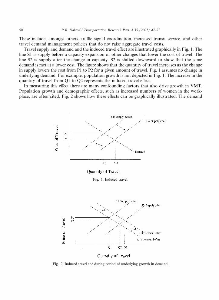
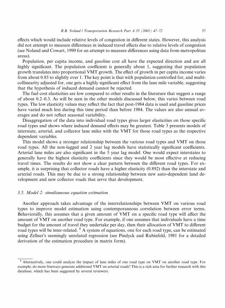
These include, amongst others, tra�c signal coordination, increased transit service, and othertravel demand management policies that do not raise aggregate travel costs.

Travel supply and demand and the induced travel e�ect are illustrated graphically in Fig. 1. Theline S1 is supply before a capacity expansion or other changes that lower the cost of travel. Theline S2 is supply after the change in capacity. S2 is shifted downward to show that the samedemand is met at a lower cost. The ®gure shows that the quantity of travel increases as the changein supply lowers the cost from P1 to P2 for a given amount of travel. Fig. 1 assumes no change inunderlying demand. For example, population growth is not depicted in Fig. 1. The increase in thequantity of travel from Q1 to Q2 represents the induced travel e�ect.

In measuring this e�ect there are many confounding factors that also drive growth in VMT.Population growth and demographic e�ects, such as increased numbers of women in the work-place, are often cited. Fig. 2 shows how these e�ects can be graphically illustrated. The demand

Fig. 1. Induced travel.

Fig. 2. Induced travel the during period of underlying growth in demand.


curve shifts outward from D1 to D2 because more travel is demanded at a given price whenpopulation increases in an area. The demand and supply curves shift simultaneously in Fig. 2, andthe resulting quantity of travel increases even more than in Fig. 1 (to Q3). Empirically, it isdi�cult to isolate these two concurrent e�ects, and this is what causes some of the uncertaintyabout the magnitude of the induced travel e�ect, as distinct from the growth e�ect. In Fig. 2, theinduced travel e�ect is measured along the horizontal axis as the di�erence between Q2 and Q1,while the e�ect from exogenous growth is the di�erence between Q3 and Q2. 1

Much of the debate over induced travel and its impact has often been confused by disagree-ments over its de®nition. For example, some would argue that only direct behavioral changes thatgenerate new trips should be called induced travel. Others may claim that shifts between modes donot generate new trips and therefore cannot be called induced travel (despite the increase inVMT). The de®nition adopted here seeks clarity in these concepts by broadly de®ning inducedVMT as any infrastructure change that results in either short run or long run increases in VMT.Hills (1996) provides a useful categorization of the various behavioral e�ects one can expect fromhighway upgrades or capacity expansions. This was used by the SACTRA (1994) study to alsode®ne induced travel very broadly.

Di�erent behavioral e�ects can be expected in the short run and in the long run. Short rune�ects that occur include changes in travel departure times, route switches, mode switches,longer trips, and some increase in trip generation. Of these, mode switches and new trips clearlycontribute to induced vehicle travel. The inability of increased capacity to reduce congestion ismost visible during peak travel times and is due to travelers shifting to preferred departuretimes. This e�ect does not represent increased VMT and so would not represent inducedtravel. 2 However, shifts to the peak that free up capacity at other times of the day can result innew trips being made at those times that are now less congested. Route switching can result ineither shorter or longer distances being traveled. If the net e�ect is more travel, this is clearlyde®ned as induced VMT. If speeds are now faster, some additional long trips (perhaps recre-ational in nature or to more distant shopping centers) are likely to be taken and clearlyrepresent induced travel.

Longer run e�ects are related to how land use patterns adjust to the newly available capacityand the resulting spatial allocation of activities. If speeds are higher, many residences and busi-nesses will tend to relocate over time often resulting in longer distance trips (Gordon and Rich-ardson, 1994). 3 The concentration of retail activities in ``big box'' stores or auto-dependentregional shopping centers (rather than centrally located business districts) further increases VMT.These are longer run e�ects that can be included in the de®nition of induced travel since they arethe result of economic changes induced by capacity additions.

1 The relative scale of the e�ects in Fig. 2 do not necessarily represent actual magnitudes.2 Peak shifting that does not noticeably reduce aggregate travel times does suggest that the bene®ts of most projects

are not accurately assessed. Rather than assessing bene®ts based on travel times an assessment based on the ability to

travel at a preferred time should be done (Small, 1992).3 While the work of Gordon and Richardson is generally meant to extoll the virtues of suburban land development

patterns, their analysis of stability in work travel times while travel speeds increase, provides good empirical evidence

for induced travel.


3. Modeling approaches and results

A variety of alternative statistical modeling approaches are presented to explore the relation-ships between lane miles of road capacity and vehicle miles of travel. These are aggregateeconometric models of VMT and lane miles. In contrast, SACTRA (1994) used a case studyapproach of before and after data for a wide selection of projects. Another technique would be touse regional travel demand models or activity-based models. These use individual level disag-gregate data from which models of individual behavior can be developed. While a disaggregateapproach is normally used for project speci®c analysis, the aggregate econometric approachadopted here provides useful information on total system e�ects.

3.1. VMT and induced travel modeling issues

Many di�erent factors a�ect total growth in VMT. Population growth naturally drives totalVMT to higher levels. Total VMT in the US grew by 3.2% annually between 1970 and 1993(DOE, 1995) exceeding total population growth (which was about 0.9% annually). Many otherdemographic factors have also been the cause of recent growth in VMT. These include, amongothers, increases in employment levels, increased female participation in the work force, andsmaller household sizes. These are all highly correlated with population increases and thereforetheir impacts cannot be separated from overall trends in population growth. Population by stateshould serve as an adequate proxy for many of these demographic e�ects. Another factor in¯u-encing VMT growth is the increase in vehicle licensing rates and the saturation of vehicle own-ership in the US. The 1995 Nationwide Personal Transportation Survey (US DOT, 1997a) resultsshow that only 8 million US households do not own a motor vehicle and over 40 millionhouseholds own two vehicles. This variable is not used in the analysis due to high collinearity withpopulation. Changes in per capita income also a�ect total VMT (and is a signi®cant factor asdiscussed in the following sections.).

The total cost of travel plays a role in demand for vehicle travel and is the basic premise of thetheory of induced travel. The major factor a�ecting the cost of travel is the value of time asso-ciated with travel. Several studies have documented the value of travel time (Small, 1992; Waters,1992). Goodwin (1992) reviewed elasticity estimates derived from studies based upon fuel prices.Tolls also a�ect total cost but are not included in the analysis due to their negligible role in the US.

Spatial reorganization of urban areas and increased concentration of many retail activities mayalso be increasing VMT. The 1995 NPTS shows that 77% of person-miles of travel is now for non-commute trips. Much of this increase may be related to increased decentralization and the de-velopment of more auto-dependent communities, which are endogenous to the development ofnew road capacity.

There is often confusion over how changes in road supply can a�ect behavior. For example,some might argue that reductions in transit usage have been a factor resulting in increased VMT,independent of changes in road supply. Other research, however, shows how reductions in transitservice can occur because of increases in road supply (Noland, 1999). This e�ect, known as theDowns±Thomson paradox results when an increase in road supply makes traveling by autopreferable to transit alternatives. The transit agency then needs to either raise fares or reduceservice; this results in a further decrease in transit usage and perhaps even worse congestion than


before the capacity expansion (Arnott and Small, 1994). Changes in many other apparently socio-economic trends could, in theory, be attributed to reduced transportation costs from road ex-pansion.

One issue that cannot be completely resolved with a statistical analysis is the issue of causality.Does VMT growth cause more lane miles to be built or does capacity expansion induce VMT?The analysis presented here strongly supports the hypothesis of induced travel. The use of a ®xede�ects cross-sectional time series model minimizes any simultaneity bias in the data (although itdoes not necessarily eliminate it). An ideal technique for resolving the causality debate would beto use an instrumental variables approach. If another variable can be found that is correlated withlane miles, but is orthogonal to VMT, then this would be possible. Several variables were exploredduring the course of this research in an attempt to ®nd an appropriate instrument. However, allthe variables that may correlate with lane miles also tend to be correlated with VMT. 4 Regardlessof these limitations, the overall robustness of the results (presented below) using di�erent for-mulations of the model, support the hypothesis of induced travel.

Many transportation professionals will argue that induced travel only demonstrates thathighway planners have put the roads where people want to travel, i.e., they have made accurateforecasts. Or alternatively, induced travel provides bene®ts since people obviously want to travel.These bene®ts must be weighed against any social costs associated with the new capacity. This isbeyond the scope of the current paper but is certainly a rich area for future research.

3.2. Data

To empirically measure induced travel e�ects it is necessary to separate the in¯uences of thevarious factors driving VMT growth. To isolate the impact of road supply, i.e., lane miles, severalmodels are formulated. The data are a cross-sectional time series (panel data) of the 50 US statesbetween the years 1984 and 1996. The District of Columbia is omitted from the data set since itdoes not have the characteristics of a typical state and was an obvious outlier. Delaware wasomitted from the simultaneous equation models since it did not have one category of road type(rural interstates). The data for VMT and lane miles for each state over the 13 year period wascollected from the Highway Statistics series published by the Federal Highway Administration(for example, see US DOT, 1997b,c).

Total lane mile growth over this 13 year period has only been about 1.25% and the total routemiles grew by about 0.71%. Excluding local roads, these ®gures are about 3.13% and 1.73%,respectively. About one quarter of new lane miles is from new roads while three quarters is ex-pansion of existing roads. There are major di�erences between di�erent road categories. 5 In-terstate and freeway lane miles have grown by about 8.98% of which about 16% is for new roads.Arterial lane miles have grown by about 11.01% of which about 32.80% is for new roads. Col-lector lane miles and route miles have actually declined slightly (1.64% and 1.56%, respectively),

4 Hansen and Huang (1997) were also unable to ®nd an appropriate instrument in their analysis.5 As de®ned in U.S. DOT (1997c) these are interstate highways, arterial roads (which include some controlled access

highways) but are generally uncontrolled, collector facilities that collect and disperse tra�c between arterials and lower

grade facilities, and local roads that distribute tra�c to actual destinations.


probably due to reclassi®cation as higher or lower order roads. Despite this relatively smallgrowth in lanes miles (due partly to the large existing network) VMT has grown at about 3.2% peryear.

Other variables included in the model include state population, per capita income by state, andthe cost per energy unit (million BTUs) of gasoline (US DOE, 1994). 6 The latter was based onaverage rates in each state for each year adjusted to constant dollars. State population is from USDOC (1997a) and per capita income in real dollars is from US DOC (1997b). During developmentof the model various other demographic variables were examined. Many of these tend to havehigh collinearity with population, such as state driver and vehicle licensing rates. A variety ofstatistical approaches, discussed below, were estimated.

3.3. General modeling approach

The general modeling approach estimates models of the following form:

log VMTitr� � � c� ai �X

k

bk log X kit

ÿ �� k log LMitrl� � � eit:

The parameters are de®ned as:

The model is estimated with di�erent road types as de®ned by U.S. DOT (1997c) and referencedabove. Both VMT and lane mile data are analyzed for all road types except local roads. 7 The datawere further disaggregated by urban and rural classi®cations. Rural roads are de®ned as areaswith a population below 5000, which might not strictly represent all areas usually consideredrural. Some roads were obviously reclassi®ed from rural to urban over the course of the timeseries.

When using lane miles as a proxy for travel cost it is necessary to lag the variable. This is neededto allow individual behavior to respond to changes in highway capacity. Hansen and Huang

VMTitr VMT in state i, for year t, by road type rc constant termai ®xed e�ect for state i, to be estimatedbk coe�cients to be estimated (for demographic and other parameters)k coe�cient to be estimated for LM parameterXk

it value of demographic and other variables for state, i, and time, tLMitrl proxy for cost of travel time (lane miles) by state, i, for year, t, for road type, r, lagged

by l yearseit random error term

6 Data for 1995 and 1996 were collected from the Petroleum Marketing Annual (U.S. DOE, 1997). These data do not

include fuel taxes which were added from U.S. DOT (1997c).7 Local roads make up the bulk of nationwide lane miles but relatively little of total VMT. Preliminary analysis

including local roads showed they were not signi®cant in inducing VMT. This is not particularly surprising since they

are used primarily for access to destinations, not for major amounts of travel between destinations.


(1997) found that lags of about 2±4 years gave good results for their estimations. Anothertechnique, discussed further below in the section on distributed lag models, is to use a model thatcaptures both long run and short run lag e�ects. Long run lags should represent cumulativeimpacts that occur over time. Inclusion of only one lag would not capture all the impacts frommultiple years.

The analysis is focused primarily on estimating the statistical signi®cance and magnitude of theelasticity of VMT with respect to lane miles. An elasticity provides a measure of how a change inone variable (lane miles) results in a a change in another response variable (VMT). For example,an elasticity of VMT with respect to lane miles of 0.5 would imply that a 1% increase in lane mileswill result in a 0.5% increase in VMT. The elasticity is just the coe�cient of the log of thatvariable, thus a logarithmic speci®cation is used in the regression analysis. This is described simplyas

� o log�VMT�o log�LM� �

LMVMT

� o�VMT�o�LM� ;

where k is the elasticity and is also the estimated coe�cient in the model.Logarithmic transformations also minimize any heteroskedasticity in the cross-sectional data

from combining states with large di�erences in size or population. The logarithmic transformationdoes not change the relative signi®cance of the results compared to a linear formulation but doesallow for an easier interpretation of the elasticity coe�cients.

The model is speci®ed as a ``®xed e�ects'' or dummy variable model (Judge et al., 1985). Es-sentially the model includes a dummy variable for each state and is estimated as an ordinary leastsquares (OLS) model. The inclusion of a dummy variable for each state allows unmeasuredfactors a�ecting the dependent variable that are associated with each state to be controlled for.The intercept coe�cient for each state is independently ®xed while the slope is estimated to be thesame across states. That is, this model assumes that all states respond to lane mile increases (andchanges in other exogenous variables) with the same behavior. An alternative formulation knownas the random e�ects model would allow each state to have not only a di�erent intercept coef-®cient but individual slope coe�cients. Selected usage of the Hausman test rejected this as areasonable hypothesis for this model (Judge et al., 1985).

The use of both population and lane miles as independent variables can cause a multi-collin-earity problem. To correct this problem, lane miles per capita are used in the following models.This reduced the largest correlations which were for urban lane miles from high values above 0.95to virtually no correlation. Interestingly the rural lane mile per capita variables have a highercorrelation with population than when not calculated as per capita variables, but the level ofcorrelation is still not a problem. Correlations for unlagged lane mile variables and per capita lanemile variables are shown in Table 1. The growth model discussed below further eliminates mostproblems with multicollinearity in the independent variables.

Alternatively, one could also estimate models with VMT per capita as the dependent variablewhile omitting population as an explanatory variable. The general results would not di�er (see, forexample, Table 8). The decision was made to regress on total VMT primarily because it allows adecomposition of population e�ects on total VMT growth. Many critics of the theory of inducedtravel attribute population growth and demographic change as being the only factors drivingVMT growth. It is hoped that this analysis will resolve these criticisms of the theory.


3.4. Model 1: aggregate data on road types

The initial model estimated sums the road types and VMT to determine whether total VMT(excluding VMT on local roads) can be explained by increases in total non-local lane miles (thatis, the sum of interstate, arterial, and collector lane miles). The results, shown in Table 2, showthat lane miles are a statistically signi®cant determinant of VMT, except in the model with a 2 yearlag. The elasticities are about 0.25, suggesting that a 0.25% increase in non-local VMT occurs forevery 1% increase in non-local lane miles. There does not appear to be a clear trend suggestingthat elasticities increase or decrease when lags are modeled, though the 2 year lag model is sig-ni®cant at the 90% level of con®dence. The estimated coe�cients take into account state speci®c

Table 2

Total VMT regressionsa

Lane miles are total non-local lane miles per capita Dependent variable is log of total non-local VMT

(A) (B) (C)

LN (lane miles per capita) 0.287

(4.167)

LN (lane miles per capita, 2 year lag) 0.166

(1.794)

LN (lane miles per capita, 5 year lag) 0.258

(4.043)

LN (population) 1.074 0.989 1.207

(16.229) (10.769) (17.003)

LN (per capita income) 1.075 1.116 0.853

(27.341) (25.805) (17.879)

LN (cost per BTU of fuel) )0.126 )0.192 )0.126

()8.025) ()6.517) ()6.030)

Constant )15.054 )14.557 )14.989

()19.883) ()16.102) ()21.733)

R2 0.898 0.876 0.891

N 650 550 400a Note that state speci®c constants are omitted for brevity. T-stats are in parentheses.

Table 1

Correlation of lane miles with population

Lane miles Lane miles per capita

Total non-local lane miles 0.6607 )0.6176

Interstate lane miles 0.7941 )0.7463

Arterial lane miles 0.8007 )0.5903

Collector lane miles 0.5328 )0.5842

Urban interstate lane miles 0.9568 0.2343

Urban arterial lane miles 0.9712 0.1974

Urban collector lane miles 0.9615 )0.0806

Rural interstate lane miles 0.3883 )0.6198

Rural arterial lane miles 0.5151 )0.5857

Rural collector lane miles 0.4303 )0.5499


e�ects which would include relative levels of congestion in di�erent states. However, this analysisdid not attempt to measure di�erences in induced travel e�ects due to relative levels of congestion(see Noland and Cowart, 1999 for an attempt to measure di�erences using data from metropolitanareas).

Population, per capita income, and gasoline cost all have the expected direction and are allhighly signi®cant. The population coe�cient is generally about 1, suggesting that populationgrowth translates into proportional VMT growth. The e�ect of growth in per capita income variesfrom about 0.85 to slightly over 1. The key point is that with population controlled for, and multi-collinearity adjusted for, one gets a highly signi®cant e�ect from the lane mile variable, suggestingthat the hypothesis of induced demand cannot be rejected.

The fuel cost elasticities are low compared to other results in the literature that suggest a rangeof about 0.2±0.3. As will be seen in the other models discussed below, this varies between roadtypes. The low elasticity values may re¯ect the fact that post-1984 data is used and gasoline priceshave varied much less during this time period than before 1984. The values are also annual av-erages and do not re¯ect seasonal variability.

Disaggregation of the data into individual road types gives larger elasticities on those speci®croad types and shows where induced demand e�ects may be greatest. Table 3 presents models ofinterstate, arterial, and collector lane miles with the VMT for those road types as the respectivedependent variables.

This model shows a stronger relationship between the various road types and VMT on thoseroad types. All the non-lagged and 2 year lag models have statistically signi®cant coe�cients.Arterial lane miles are also signi®cant in the 5 year lag model. One would expect interstates togenerally have the highest elasticity coe�cients since they would be most e�ective at reducingtravel times. The results do not show a clear pattern between the di�erent road types. For ex-ample, it is surprising that collector roads have a higher elasticity (0.892) than the interstate andarterial roads. This may be due to a strong relationship between new auto-dependent land de-velopment and new collector roads that serve that development.

3.5. Model 2: simultaneous equation estimation

Another approach takes advantage of the interrelationships between VMT on various roadtypes to improve model estimation using contemporaneous correlation between error terms.Behaviorally, this assumes that a given amount of VMT on a speci®c road type will a�ect theamount of VMT on another road type. For example, if one assumes that individuals have a timebudget for the amount of travel they undertake per day, then their allocation of VMT to di�erentroad types will be inter-related. 8 A system of equations, one for each road type, can be estimatedusing ZellnerÕs seemingly unrelated regression (see Pindyck and Rubinfeld, 1981 for a detailedderivation of the estimation procedure in matrix form).

8 Alternatively, one could analyze the impact of lane miles of one road type on VMT on another road type. For

example, do more freeways generate additional VMT on arterial roads? This is a rich area for further research with this

database, which has been suggested by several reviewers.


Table 3

VMT regressions by road typea

Lane miles per capita are by road type Dependent variable is log of VMT by road type

(A) (B) (C) (D) (E) (F) (G) (H) (I)

LN (interstate lane miles per capita) 0.627

(10.129)

LN (interstate lane miles 2 year lag, per capita) 0.549

(8.026)

LN (interstate lane miles 5 year lag, per capita) 0.043

(0.547)

LN (arterial lane miles, per capita) 0.632

(14.779)

LN (arterial lane miles 2 year lag, per capita) 0.268

(5.366)


(2.996)

LN (colector lane miles, per capita) 0.892

(12.326)

LN (collector lane miles 2 year lag, per capita) 0.542

(5.132)


(0.909)

LN (population) 1.376 1.374 1.123 1.243 1.069 1.249 1.180 0.968 0.569

(18.543) (15.836) (10.682) (24.661) (16.293) (15.628) (10.927) (6.046) (2.548)

LN (per capita income) 1.462 1.474 1.399 0.835 0.938 0.805 0.911 0.706 0.332

(26.969) (23.602) (16.357) (19.216) (17.766) (12.250) (11.846) (7.477) (2.276)

LN (cost per BTU of fuel) )0.178 )0.231 )0.228 )0.099 )0.212 )0.149 )0.086 )0.064 0.018

()8.530) ()5.861) ()6.334) ()6.334) ()5.829) ()5.090) ()2.840) ()0.965) (0.274)

Constant )21.473 )21.984 )20.889 )13.768 )13.922 )15.985 )13.638 )10.266 )2.642

()27.527) ()25.962) ()20.306) ()21.382) ()21.382) ()18.254) ()9.978) ()5.505) ()1.178)

R2 0.908 0.885 0.844 0.869 0.815 0.817 0.538 0.324 0.112

N 650 550 400 650 550 400 650 550 400a Note that state speci®c constants are omitted for brevity. T-stats are in parentheses.

58

R.B

.N

ola

nd

/T

ran

spo

rtatio

nR

esearch

Pa

rtA

35

(2

00

1)

47

±7

2

The disturbance covariance matrix in this model is assumed to be non-diagonal because of therelationships between the equations. This technique produces lower standard errors by takingadvantage of the contemporaneous correlation between the error terms. In other words, the errorterm associated with an equation estimated for a speci®c road type (e.g. urban interstates) iscorrelated with the error term for rural arterials. This information allows a more e�cient esti-mator for the coe�cients to be derived.

Results are shown in Table 4. Coe�cient values for the lane mile parameters are generallylarger and show increased statistical signi®cance. Both the models with no lag and with the 2 yearlag show that all increases in lane miles are related to an increase in VMT (all are statisticallysigni®cant at the 95% con®dence level). The no lag interstate lane mile coe�cient shows anelasticity of 0.713, the arterial no lag model has an elasticity of 0.690, and the collector no lagmodel has an elasticity of 0.826. The elasticity values are smaller in the 2 year lag model. Theelasticities are 0.567, 0.267 and 0.509 for interstates, arterials, and collectors, respectively. Otherthan for arterials, the 5 year lag model lane mile coe�cients are not signi®cant.

This model would seem to suggest the largest immediate and short-term (up to 2 years) e�ectfrom adding interstate and collector lane miles. On the other hand, while arterial lane miles seemto generate less VMT, the e�ect persists over a longer time period (at least up to 5 years). Theremay be some intuitive reasoning behind these results. First, new construction and expansion ofinterstates may result in large immediate e�ects from relatively large reductions in travel costs.Construction of collector lane miles may mirror the construction of new developments that theymay serve, also generating some immediate increases in VMT. Arterials, on the other hand, mayrespond slower as land use patterns respond to lower travel costs on arterials. These are, ofcourse, merely speculations as to what may be driving di�erences in the coe�cient values, but dosuggest areas where more detailed analysis could be pursued.

The other coe�cients also show some interesting e�ects. The fuel cost coe�cient is generallysigni®cant with a negative sign. It is largest for the interstate VMT models, somewhat lower forthe arterial VMT models, and much lower for the collector VMT models. The longer distancestravelled on interstates probably accounts for the larger elasticity of fuel costs with respect tointerstate VMT. These trips may be more discretionary or have substitutes (such as shorter tripsto local destinations). Collector roads, which are not used for longer distance travel show thesmallest fuel cost elasticity, and may re¯ect the less discretionary travel involved in access todestinations.

The same elasticity di�erence is apparent with respect to per capita income. Per capita incomegenerally has an elasticity greater than (or nearly equal to) 1 with respect to interstate VMT.Increases in income may result in more leisure travel (on interstates) and longer commutingdistances (on interstates) as people move to more distant suburbs.

A further disaggregation of the data can be achieved by breaking out urban and rural VMT andlane miles for each road class. The simultaneous equation model for this set of six equations isshown in Table 5 with no lag and in Table 6 for a 5 year lag. The rural road categories haverelatively high collinearity which may somewhat bias the results on these coe�cients. The no lagmodel shows very large elasticities for all the lane mile variables. They range from a low of 0.325for rural interstates up to 0.773 for rural collectors. The urban lane mile elasticities are all above0.7. The 5 year lag model (Table 6) shows signi®cance only for urban interstates and arterials andrural arterials. Surprisingly the rural interstate coe�cient is negative, although it is below the 90%


Table 4

Seemingly unrelated regression by road typea

Lane miles per capita are by road type Dependent variable is log of VMT by road type

Model 1: no lag Model 2: 2 year lag Model 3: 5 year lag

(A) (B) (C) (D) (E) (F) (G) (H) (I)

LN (interstate lane miles per capita) 0.713

(13.139)

LN (arterial lane miles per capita) 0.690

(18.991)

LN (collector lane miles per capita) 0.826

(12.177)

LN (interstate lane miles 2 year lag, per

capita)

0.567

(8.709)


(5.720)


(5.023)

LN (interstate lane miles 5 year lag, per

capita)

0.064

(0.812)


(2.848)


(0.816)

LN (population) 1.442 1.265 1.118 1.389 1.073 0.933 1.138 1.245 0.555

(20.423) (25.442) (10.613) (16.329) (16.402) (5.943) (10.834) (15.578) (2.486)

LN (per capita income) 1.439 0.832 0.901 1.467 0.936 0.706 1.388 0.807 0.335

(26.832) (19.151) (11.731) (23.728) (17.759) (7.481) (16.241) (12.283) (2.298)

LN (cost per BTU of fuel) )0.174 )0.097 )0.086 )0.229 )0.212 )0.065 )0.225 )0.149 0.017

()8.348) ()5.586) ()2.844) ()5.824) ()5.834) ()0.981) ()6.253) ()5.102) (0.265)

Constant )17.238 )13.802 )13.655 )21.719 )13.781 )10.348 )20.105 )15.388 )3.094

()23.135) ()23.988) ()11.007) ()28.951) ()19.811) ()6.172) ()22.446) ()20.165) ()1.525)

N 650 650 650 550 550 550 400 400 400a Note that state speci®c constants are omitted for brevity. T-stats are in parentheses.

60

R.B

.N

ola

nd

/T

ran

spo

rtatio

nR

esearch

Pa

rtA

35

(2

00

1)

47

±7

2

level of signi®cance. Overall these results demonstrate a strong induced travel e�ect with somedi�erentiation between di�erent road types that merits further investigation.

3.6. Model 3: distributed lags

The previous models suggest that the short-term elasticity of lane miles with respect to VMT isgreater in the ®rst year than for subsequent years. However, in theory, one would expect a cu-mulative impact where the increase in VMT adjusts over time. The previous models only estimatea single lag and do not take into account this cumulative impact.

One technique for estimating a long-term elasticity is a distributed lag model using a lagged-dependent variable (Johnston, 1984). This technique, known as partial adjustment, has beenapplied to shocks in the price of gasoline and its e�ect on consumption over time. In the short run,gasoline consumption is reduced by cancellation of some trips and shorter trips, while in the longrun fuel e�ciency is increased. The case of increased road capacity has some parallels in that theadjustment process is hypothesized to take place over time with both short run and long rune�ects. This technique is relatively simple to apply but does assume that the adjustment processfrom the other independent variables, population, personal income, and gasoline prices, is thesame as for lane mileage. It also assumes an exponential pattern to the lag, which may be fairlyrealistic in this case.

Table 5

Seemingly unrelated regression by road type and urban/rural area, no lag modela

Lane miles are by road type per capita Dependent variable is log of VMT by road type

Urban

interstates

Urban

arterials

Urban

collectors

Rural

interstates

Rural

arterials

Rural

collectors

LN (urban interstate lane miles, per capita) 0.738

(29.542)

LN (urban arterial lane miles, per capita) 0.712

(29.225)

LN (urban collector lane miles, per capita) 0.749

(19.196)

LN (rural interstate lane miles, per capita) 0.325

(6.526)

LN (rural arterial lane miles, per capita) 0.610

(16.236)

LN (rural collector lane miles, per capita) 0.773

(10.612)

LN (population) 1.391 1.119 1.084 0.620 0.979 0.809

(22.281) (20.475) (8.725) (6.958) (15.327) (6.440)

LN (per capita income) 1.398 0.731 1.035 1.639 1.162 0.732

(24.000) (14.686) (9.092) (25.112) (22.119) (8.485)

LN (cost per BTU of fuel) )0.144 )0.077 )0.006 )0.199 )0.026 )0.134

()6.314) ()3.823) ()0.135) ()7.635) ()1.261) ()3.934)

Constant )20.716 )10.517 )13.894 )14.719 )14.113 )8.251

()24.401) ()15.274) ()8.979) ()15.141) ()19.523) ()5.528)

N 632 632 632 632 632 632a Note that state speci®c constants are omitted for brevity. T-stats are in parentheses.


The speci®cation for the distributed lag model is

log VMTitr� � � c log VMTi�tÿ1�rÿ �� c� ai �

Xk

bk log X kit

ÿ �� k log LMitr� � � eit:

All variables are as de®ned previously. The only di�erence is the lagged VMT term with acoe�cient c.

Short run elasticities of lane miles with respect to VMT correspond to the coe�cient on the lanemile variable, k. Long run elasticities can be calculated as

g � k1ÿ c

:

The adjustment parameter, c, is the coe�cient on the lagged VMT variable as de®ned above(Johnston, 1984).

Distributed lag models were estimated with both aggregate VMT and lane mile data and withsimultaneous equations disaggregated by road type. Table 7 shows two aggregate distributed lagmodels. One problem with including lagged VMT is that it is collinear with population and lanemiles. The ®rst model in Table 7 includes population despite this problem. The second modelremoves population and has VMT per capita as the dependent variable. The coe�cient estimates

Table 6

Seemingly unrelated regression by road type and urban/rural area, 5 year lag modela

Lane miles are by road type,

lagged 5 years, per capita

Dependent variable is log of VMT by road type

Urban

interstates

Urban

arterials

Urban

collectors

Rural

interstates

Rural

arterials

Rural

collectors

LN (urban interstate lane miles,

lagged 5 years, per capita)

0.141

(2.099)

LN (urban arterial lane miles,


0.097

(2.732)

LN (urban collector lane miles,


0.004

(0.049)

LN (rural interstate lane miles,


)0.098

()1.842)

LN (rural arterial lane miles,


0.336

(3.322)

LN (rural collector lane miles,


0.117

(0.620)

LN (population) 1.795 1.302 2.274 0.265 1.124 )0.500

(13.181) (13.212) (8.436) (2.414) (7.005) ()1.799)


(12.320) (8.505) (1.286) (14.949) (7.484) (2.833)


()6.613) ()5.846) ()1.127) ()3.089) ()0.158) ()0.011)

Constant )30.664 )16.278 )26.639 )9.511 )14.369 8.662

()19.394) ()15.097) ()9.625) ()9.194) ()10.310) (3.409)



do not appear to be a�ected by the collinearity. The elasticities for the two estimated equations aregenerally similar. Long run elasticities are substantially larger than the short run elasticities as onewould expect.

Tables 8 and 9 present two similar analyses using a simultaneous equation framework. Table 8omits population as an independent variable and uses VMT per capita as the dependent variable.Table 9 includes population and VMT as the dependent variable. Lagged VMT is highly collinearwith population, however the similarity of the coe�cients with and without the populationvariable suggests that multi-collinearity is not creating a large bias in the model in Table 9. Boththese models have large long run elasticities in the range 0.7±1.0 (exceeding 1.0 for collectorroads). Short run elasticities are also substantial, in the range of 0.2±0.5. Short run elasticities arelarger for urban road categories than for rural roads, perhaps due to more congestion in urbanareas. Long run elasticities are about the same for both urban and rural roads. This would suggestthat capacity increases are triggering fundamental land use changes that increase VMT in bothurban and rural areas. Similar to some of the other models, collector roads again have relativelylarge elasticities (exceeding 1.0 for the long run elasticities). This may imply a strong relationshipbetween adding collector roads and subsequent new development that generates new trips. Ruralinterstates have the smallest short run elasticities. This suggests that long distance travel does notrespond as quickly to capacity increases (or that rural interstates are less congested).

Population is also a signi®cant factor with larger coe�cients in the urban equations. Per capitaincome is signi®cant across equations with smaller coe�cients on collector roads. This maysuggest some base level of travel that is not related to income while the use of interstates andarterial roads is a�ected more by income levels. Gasoline price coe�cients are generally small.

Table 7

Total VMT regression (distributed lag modelsa)

Dependent variable LN

(non-local VMT)

LN

(non-local VMT per capita)

LN (lane miles per capita) 0.119 0.128

(2.680) (4.250)

LN (VMT lagged one year) 0.674 ±

(27.226)

LN (VMT per capita lagged one year) ± 0.690

(27.928)

LN (population) 0.304 ±

(5.851)

LN (per capita income) 0.376 0.321

(9.982) (8.479)

LN (cost per BTU of fuel) )0.048 )0.049

()4.017) ()4.124)

Constant )4.316 )3.995

()6.734) ()8.927)

R2 0.953 0.913

N 600 600

Short run elasticity 0.119 0.128

Long run elasticity 0.365 0.413a Note that state speci®c constants are omitted for brevity. T-stats are in parentheses.


They are insigni®cant for collector roads, again suggesting that base VMT is una�ected by gas-oline prices.

These results are similar to the results of Tables 5 and 6. However, the previous method thatincorporated only one 5 year lag did not fully account for the cumulative impact of long-terme�ects as this method does. The distributed lag models also have smaller coe�cient values on thedemographic variables since they are short run e�ects. The long run elasticities for these corre-spond fairly closely with the estimates in Tables 5 and 6.

One criticism of distributed lag models is that they are highly unstable in providing goodpredictions. Almon (1989) suggests a procedure for comparing the actual values with predictedvalues over the sampling period. Forecasts of VMT are calculated for each year using the datafor each year plus a forecasted lagged value of VMT. Fig. 3 shows a very good ®t for themodel in Table 9 between predicted total VMT and actual total VMT. Rural and urbancollector predictions are the least stable (comparatively) but represent a minor fraction of thetotal VMT.

Table 8

Seemingly unrelated regression by road type and urban/rural area (distributed lag model, per capita VMTa)

Lane miles are by road type per capita Dependent variable is log of VMT per capita by road type

Urban

interstates

Urban

arterials

Urban

collectors

Rural

interstates

Rural

arterials

Rural

collectors

LN (VMT per capita, lagged one year) 0.492 0.379 0.529 0.675 0.487 0.653

(19.878) (13.303) (20.056) (30.810) (16.753) (21.715)


(16.784)


(17.794)


(14.990)


(9.204)


(11.382)


(8.774)


(11.730) (10.269) (4.965) (9.086) (11.941) (4.003)


()4.245) ()2.403) ()0.685) ()3.609) ()1.847) ()1.181)

Constant )7.532 )5.448 )4.092 )4.942 )7.162 )3.440

()10.402) ()9.818) ()4.369) ()8.864) ()12.165) ()4.915)

N 583 583 583 583 583 583

Long run elasticities

Lane miles per capita 0.841 0.791 1.087 0.794 0.706 1.216

Personal income 1.406 0.763 0.858 1.428 1.172 0.784

Gasoline price )0.167 )0.079 )0.057 )0.200 )0.070 )0.104a Note that state speci®c constants are omitted for brevity. T-stats are in parentheses.


Fig. 3. Comparison of predicted and actually VMT using distributed lag model.

Table 9

Seemingly unrelated regression by road type and urban/rural area (distributed lag modela)

Lane miles are by road type per capita Dependent variable is log of VMT by road type

Urban

interstates

Urban

arterials

Urban

collectors

Rural

interstates

Rural

arterials

Rural

collectors

LN (VMT, lagged one year) 0.464 0.370 0.528 0.669 0.485 0.649

(17.981) (12.915) (20.251) (30.774) (16.658) (21.658)


(17.136)


(18.002)


(15.097)


(6.473)


(10.621)


(6.726)

LN (population) 0.625 0.652 0.690 0.250 0.509 0.307

(9.561) (10.279) (6.645) (4.057) (8.159) (2.950)


(12.227) (9.788) (3.545) (9.858) (11.450) (4.387)


()4.191) ()2.308) ()0.478) ()3.590) ()1.746) ()1.106)

Constant )9.149 )5.908 )6.219 )4.702 )7.349 )3.350

()9.479) ()7.864) ()4.907) ()6.574) ()10.093) ()2.786)

N 583 583 583 583 583 583

Long run elasticities

Lane miles per capita 0.819 0.790 1.087 0.707 0.717 1.160

Population 1.166 1.035 1.462 0.755 0.988 0.875

Personal income 1.396 0.776 0.695 1.604 1.223 0.892

Gasoline price )0.159 )0.075 )0.040 )0.193 )0.068 )0.094a Note that state speci®c constants are omitted for brevity. T-stats are in parentheses.


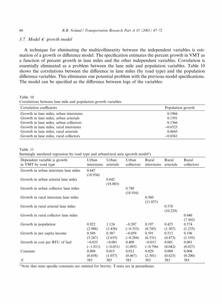
3.7. Model 4: growth model

A technique for eliminating the multicollinearity between the independent variables is esti-mation of a growth or di�erence model. The speci®cation estimates the percent growth in VMT asa function of percent growth in lane miles and the other independent variables. Correlation isessentially eliminated as a problem between the lane mile and population variables. Table 10shows the correlations between the di�erence in lane miles (by road type) and the populationdi�erence variables. This eliminates one potential problem with the previous model speci®cations.The model can be speci®ed as the di�erence between logs of the variables:

Table 10

Correlations between lane mile and population growth variables

Correlation coe�cients Population growth

Growth in lane miles, urban interstates 0.1966

Growth in lane miles, urban arterials 0.1591

Growth in lane miles, urban collectors 0.1366

Growth in lane miles, rural interstates )0.0325

Growth in lane miles, rural arterials 0.0643

Growth in lane miles, rural collectors )0.0361

Table 11

Seemingly unrelated regression by road type and urban/rural area (growth modela)

Dependent variable is growth

in VMT by road type

Urban

interstates

Urban

arterials

Urban

collectors

Rural

interstates

Rural

arterials

Rural

collectors

Growth in urban interstate lane miles 0.647

(18.936)

Growth in urban arterial lane miles 0.642

(18.083)

Growth in urban collector lane miles 0.780

(18.916)

Growth in rural interstate lane miles 0.560

(11.037)

Growth in rural arterial lane miles 0.578

(10.229)

Growth in rural collector lane miles 0.646

(7.502)

Growth in population 0.922 1.124 )0.207 0.197 0.425 0.574

(2.988) (3.436) ()0.353) (0.745) (1.307) (1.235)

Growth in per capita income 0.569 0.307 )0.059 0.591 0.513 0.196

(5.247) (2.655) ()0.284) (6.331) (4.473) (1.193)

Growth in cost per BTU of fuel )0.035 )0.001 0.409 )0.013 0.001 0.001

()1.811) ()0.051) (1.095) ()0.796) (0.042) (0.027)

Constant 0.009 0.015 0.012 0.029 0.009 0.004

(0.658) (1.037) (0.467) (2.501) (0.625) (0.200)



log VMTitr� � ÿ log VMTi�tÿ1�rÿ � � c� ai �

Xk

bk log X kit

ÿ ��ÿ log X k

i�tÿ1��

� k log LMitr� �ÿÿ log LMi�tÿ1�r

ÿ �� eit:

This corresponds to percent growth in the dependent and independent variables.The growth model also allows the testing of changes in lane miles between di�erent years and

how that might a�ect current changes in VMT. This was done for lags between two and up to ®veyears, but no signi®cant results were found. Table 11 shows results for a ®xed e�ect di�erencemodel estimated as a set of seemingly unrelated regressions. This is done with no lag which wasthe only formulation that provided a signi®cant e�ect. The results are consistent with previousspeci®cations and add support to the robustness of the relationships.

4. Importance of the induced demand e�ect

While the above results clearly demonstrate that induced travel is a likely outcome of ca-pacity expansion, many critics have asserted that demographic factors are still the overwhelmingfactor in driving increases in VMT. For example, Heanue (1998) uses the elasticity valuesgenerated by SACTRA (1994) and Hansen (1995) and calculates that capacity expansion ac-counts for somewhere between 6% and 22% of VMT growth. The conclusion reached by theauthor is that while it is necessary to account for this in investment decisions and cost-bene®tanalysis the overall importance of induced demand is minor. One can certainly argue whether afactor that may cause up to 22% of VMT growth should be considered minor, but arguments ofthis type tend to obfuscate the issue. The key question is the relative social costs and bene®ts ofthe additional VMT.

To address this question, the relative contribution of lane mile additions to VMT growth,relative to other factors is analyzed for some of the models above. The models estimated inTable 5 (®xed e�ects SURE model), Table 9 (distributed lag model), and Table 11 (growthmodel) are forecasted out by 5 years (from 1996 to 2001) for three di�erent scenarios. The ®rstscenario assumes that the growth rate in demographic variables (personal income, population,and gasoline costs) and lane miles by road type follows historical trends between 1992 and 1996.A second scenario assumes growth only in lane miles and no growth in the demographicvariables while the third assumes no growth in lane miles but historical growth in the demo-graphic variables.

Results for each of the models are shown in Tables 12±14. Note that for the distributed lagmodel an iterative process to generate new lag values was needed to calculate the forecast value.The full results are displayed in Fig. 4 and in Table 13.

These results are quite interesting. First, it is clear that if lane mile growth is frozen, thendemographic growth continues to drive increases in total VMT. The opposite is also true that iflane mile growth continues but demographic growth is frozen, VMT still continues to grow butnot as much. The annualized rate of total VMT growth (assuming historical growth in bothvariables) ranges from 2.65% to 2.92% for the three models. With only lane mile growth it isranges from 0.79% to 1.73% annualized VMT growth over 5 years. With just demographicgrowth the range is from 1.89% to 2.31% annualized VMT growth over 5 years. The di�erence


between this latter growth and the scenario with growth in all the variables can be attributed toadditional capacity. Therefore, if capacity is frozen at current levels, annualized VMT growthafter 5 years will be between 0.61% and 0.76% less than compared to current trends. This alsoindicates a fairly robust e�ect for the di�erent model speci®cations. The distributed lag modelforecast (see Table 13) shows both a short run (0.65% less in the ®rst year) and long run e�ect(0.76% less after ®ve years). For the distributed lag model about 28.7% (0.76/2.65) of total VMTgrowth can be attributed to growth in capacity over 5 years. In the ®rst year induced demandaccounts for 23.7% (0.65/2.74) of VMT growth in this model. For the model in Table 5 induceddemand causes 21% of VMT growth and for the model in Table 11 it accounts for 26.5% ofVMT growth.

The induced growth in VMT also has a substantial e�ect on total vehicle emissions. If weassume that 28% of the growth rate in VMT is attributable to lane miles (as estimated in thedistributed lag model), this amounts roughly to about 43 million metric tons of additional annualcarbon emissions in the year 2012. This is nearly half of the targeted carbon emissions reductionestimated for the US. Climate Change Action Plan of 90 million metric tons of carbon (by 2010).It is also equivalent to a policy of increasing the light duty vehicle ¯eet e�ciency (for gasoline) byabout 2.5% annually between 1999 and 2012 to over 47 miles per gallon. This would be virtuallyimpossible to implement even with the immediate introduction of new fuel e�cient vehicletechnologies. 9

This estimate of carbon emissions does not account for changes in levels of congestion andtra�c ¯ow dynamics that may also a�ect emissions. Emissions of criteria air pollutants (NOx, CO,

Table 12

Forecast using model in Table 5 (SURE model)

VMT forecast in 2001

VMT

urban

interstates

VMT

urban

arterials

VMT

urban

collectors

VMT

rural

interstates

VMT

rural

arterials

VMT

rural

collectors

Total

VMT

Annualized

growth rate

in VMT

Historic growth in demographic and lane mile variables

616,236 759,347 147,273 262,883 424,933 250,887 2,461,559 2.68%

Forecasted growth

rate

3.97% 2.46% 2.89% 2.49% 2.42% 0.86% 2.68%

Demographic growth only

583,396 717,622 138,810 263,236 421,576 253,180 2,377,820 1.97%

Forecasted growth

rate

2.84% 1.31% 1.68% 2.52% 2.26% 1.04% 1.97%

Lane mile growth only

548,074 710,181 134,396 230,600 382,622 238,341 2,244,213 0.79%

Forecasted growth

rate

1.56% 1.10% 1.02% )0.16% 0.29% )0.17% 0.79%

9 These estimates are based on forecasts in US DOE/EIA (1998). The VMT forecasts in this report are generally

considered conservative by EPA which uses a 2.3% annual growth rate rather than EIAÕs annual growth rate of 1.6%.

Reductions in a higher growth rate would give larger emissions bene®ts.


Table 13

Forecasts using model in Table 9 (distributed lag model)


VMT

urban

interstates

VMT

urban

arterials

VMT

urban

collectors

VMT

rural

interstates

VMT

rural

arterials

VMT

rural

collectors

TOTAL

VMT

Annualized

growth rate

in VMT


1997 530,406 691,021 131,473 237,934 387,767 242,383 2,220,984

1998 551,137 709,297 135,652 243,543 397,726 244,491 2,281,846 2.74%

1999 571,006 727,704 140,090 249,278 407,383 246,618 2,342,078 2.69%

2000 590,887 746,539 144,768 255,143 417,009 248,749 2,403,096 2.66%

2001 611,240 765,949 149,712 261,149 426,748 250,890 2,465,688 2.65%

Forecasted growth

rate

3.61% 2.61% 3.30% 2.35% 2.42% 0.87% 2.65%


1997 527,154 685,774 130,515 237,979 387,408 242,603 2,211,433

1998 542,720 696,461 133,014 243,660 396,795 245,075 2,257,727 2.09%

1999 556,215 706,084 135,242 249,482 405,743 247,656 2,300,422 1.99%

2000 568,843 715,367 137,298 255,442 414,559 250,293 2,341,802 1.93%

2001 581,198 724,599 139,263 261,544 423,404 252,968 2,382,976 1.89%

Forecasted growth

rate

2.47% 1.39% 1.64% 2.39% 2.25% 1.05% 1.89%


1997 524,646 685,558 130,669 236,112 383,682 241,480 2,202,147

1998 536,455 696,060 133,556 238,587 387,383 242,091 2,234,132 1.45%

1999 545,570 705,578 136,383 240,237 389,600 242,326 2,259,694 1.30%

2000 553,502 714,861 139,225 241,323 391,094 242,299 2,282,304 1.20%

2001 560,990 724,213 142,148 242,028 392,249 242,101 2,303,729 1.13%

Forecasted growth rate 1.69% 1.38% 2.13% 0.62% 0.55% 0.06% 1.13%

Table 14

Forecasts using model in Table 11 (growth model)


VMT

urban

interstates

VMT

urban

arterials

VMT

urban

collectors

VMT

rural

interstates

VMT

rural

arterials

VMT

rural

collectors

Total

VMT

Annualized

growth rate

in VMT


605,338 770,554 153,890 276,134 423,526 261,842 2,491,285 2.92%



578,081 733,393 146,235 276,669 420,257 263,412 2,418,047 2.31%



562,111 719,381 155,525 261,885 399,913 252,046 2,350,861 1.73%



and HC) tend to be more sensitive to these dynamics than carbon emissions. A more detailedanalysis would look at changes in these dynamics due to exogenous growth in VMT not related toinduced e�ects. However, it is also possible that relative tra�c ¯ow dynamics will be equally badbut with more tra�c if additional capacity is built.

Overall, these results suggest that if the induced travel e�ect is accounting for a quarter of VMTgrowth, that this is a highly signi®cant e�ect that needs to be measured in any defensible bene®tcost analysis or travel demand modeling exercise.

5. Conclusions

The results of the analyses presented clearly demonstrate that the hypothesis of induced de-mand cannot be rejected. Increased capacity clearly increases vehicle miles of travel beyond anyshort run congestion relief that may be obtained. The methods employed all found statisticallysigni®cant relationships between lane miles and VMT. While other factors, such as populationgrowth, also drive increases in VMT, capacity additions account for about one quarter of thisgrowth. This contribution to VMT growth has signi®cant impacts on various environmentalgoals. For example, increasing US highway capacity at historical rates may result in up to 43million metric tons of carbon emissions compared to a complete freeze on adding additional lanemiles. Constructing new lane miles at half the current rate might reduce carbon emissions pro-portionally.

The di�erent statistical approaches estimated gave a range of values for elasticity estimates. Ingeneral, more disaggregate data by road type led to relatively greater elasticity values for VMT.This is not a surprising result as many countervailing e�ects may be present in a more aggregateanalysis and the simultaneous equations may be picking up diversion e�ects between road cate-gories. Hansen and HuangÕs (1997) study found higher elasticities (up to 0.9) than the aggregateanalysis presented here which may be due to the more localized data for speci®c Californiacounties and metropolitan areas that they analyzed.

Another general e�ect is that urban roads have a greater relationship to VMT growth thansmaller rural roads. This is not too surprising since these roads are probably more congested than

Fig. 4. Forecast of VMT with demographic and lane mile e�ects using distributed lag model.


those in rural areas and would be currently suppressing some growth in tra�c if they are con-gested. Also, in general, the lagged models with one lag term show less signi®cance and smallercoe�cients than the unlagged model. This is consistent with an exponential lag function asmodeled with the distributed lag model. Cumulative long-term elasticities are greater than shortrun elasticities, as would be expected.

One surprising result is that collector roads often had a larger elasticity value than interstatesand arterials. While this cannot be clearly explained it may be due to new developments that arebuilt in conjunction with new collector road capacity.

The selection of estimation procedure can produce very di�erent results. The use of ®xed e�ectssigni®cantly reduced the level of signi®cance compared to modeling without ®xed e�ects (resultsare not shown). The latter speci®cation would be inappropriate, but is commonly used by manypractitioners. The ability to use simultaneous equations and ®xed e�ects seems to provide robustresults that take advantage of the statistical properties of the data.

Recognition of induced travel e�ects has several major policy implications. The major questionis whether the induced growth in VMT is bene®cial or not. There may be some bene®ts to pro-viding mobility and increasing access to undeveloped land, however, this must be weighed againstthe environmental and social costs associated with increases in VMT, road construction, and landdevelopment. This latter is a major issue with regard to urban development and the debate overrelatively more compact versus sprawling development patterns. The ability of planners to answerthese questions is hampered by travel demand forecasting techniques that cannot adequatelymodel these impacts at either the regional or project speci®c level (although new innovations andtechniques are beginning to be used). The other implication is that building more road capacitywill, in the long run, not solve congestion problems. While the results derived here do not strictlyprove a causal relationship between lane miles and VMT, these results still strongly suggest thatinduced demand e�ects are real and need to be considered both by planners and policy makers atboth the regional and national level.

Acknowledgements

I would like to thank Mark Corrales and Dharm Guruswamy for assistance in compiling thedata used in this analysis. Bill Cowart provided assistance with some preliminary estimates. JamesNolan and Bob Shackleton provided advice and suggestions on various estimation procedures.John Thomas provided help with carbon emissions forecasts. Additional comments from AlanKrupnick, Ken Small, Marlon Boarnet, Michael Cameron, Doug Lee, Fred Ducca, and MarkWolcott and six anonymous referees contributed to improving the paper. This work was con-ducted while the author was an analyst at the US. Environmental Protection Agency, O�ce ofPolicy. All remaining errors, omissions, and conclusions are strictly the authorÕs responsibility.

References

Almon, C., 1989. The Craft of Economic Modeling, 2nd ed. Interindustry Economic Research Fund, Ginn Press,

Needham Heights, MA.


Arnott, R., Small, K., 1994. The economics of tra�c congestion. American Scientist 82, 446±455.

Boarnet, M., 1997. Highways and economic productivity: interpreting recent evidence. Journal of Planning Literature

11, 476±486.

Coombe, D., 1996. Induced tra�c: what do transportation models tell us?. Transportation 23, 83±101.

Goodwin, P.B., 1996. Empirical evidence on induced tra�c, a review and synthesis. Transportation 23, 35±54.

Goodwin, P.B., 1992. A review of new demand elasticities with special reference to short and long run e�ects of price

changes. Journal of Transport Economics and Policy 26, 155±169.

Gordon, P., Richardson, H.W., 1994. Congestion trends in metropolitan areas. In: Curbing gridlock: Peak-period fees

to relieve tra�c congestion, volume 2, National Research Council, National Academy Press, Washington, DC,

pp. 1±31.

Hansen, M., 1995. Do Highways Generate Tra�c? Access, no. 7, University of California Transportation Center.

Hansen, M., Huang, Y., 1997. Road supply and tra�c in California urban areas. Transportation Research A 31,

205±218.

Heanue, K., 1998. Highway Capacity and Induced Travel: Issues, Evidence and Implications, Transportation Research

Circular, no. 481, Transportation Research Board, National Research Council.

Hills, P.J., 1996. What is induced tra�c?. Transportation 23, 5±16.

Johnston, J., 1984. Econometric methods. McGraw-Hill, New York.

Judge, G.G., Gri�ths, W.E., Hill, R.C., L�utkepohl, H., Lee, T., 1985. The Theory and Practice of Econometrics, 2nd

ed.. Wiley, New York.

Mackie, P.J., 1996. Induced tra�c and economic appraisal. Transportation 23, 103±119.

Noland, R.B., 1999. Modeling transit convenience: impacts on transit ridership of headway increases, paper no. 991527.

Presented at the 78th Annual Meeting of the Transportation Research Board, Washington, DC.

Noland, R.B., Cowart, W.A., 1999. Analysis of Metropolitan Highway Capacity and the Growth in Vehicle Miles of

Travel. Working paper submitted to the 79th Annual Meeting of the Transportation Research Board.

Pindyck, R.S., Rubinfeld, D.L., 1981. Econometric Models and Economic Forecasts. McGraw-Hill, New York.

SACTRA, 1994. Trunk roads and the generation of tra�c, Department of Transport, Standing Advisory Committee on

Trunk Road Assessment, London.

Small, K.A., 1992. Urban transportation economics. Harwood Academic Publishers, Chur, Switzerland.

Transportation Research Board, 1995. Expanding metropolitan highways: implications for air quality and energy use.

Special report 245, National Research Council, National Academy Press, Washington, DC.

U.S. DOC, 1997a. Annual time series of state population estimates, Bureau of the Census.

U.S. DOC, 1997b. Table SA-2, Bureau of Economic Analysis.

U.S. DOE, 1994. State energy price and expenditure report, Energy Information Administration, DOE/EIA-0376(94).

U.S. DOE, 1995. Transportation Energy Data Book, 15th ed. Oak Ridge National Laboratory, ORNL-6856.

U.S. DOE, 1997. Petroleum marketing annual, 1996, Energy Information Administration, O�ce of Oil and Gas, DOE/

EIA-0487(96).

U.S. DOE/EIA, 1998. Annual Energy Outlook 1999: with projections to 2020, Energy Information Administration,

O�ce of Integrated Analysis and Forecasting, U.S. Department of Energy, Washington, DC. DOE/EIA-0383(99).

U.S. DOT, 1995. Activity-based modeling system for travel demand forecasting, Travel Model Improvement Program,

DOT-T-96-02.

U.S. DOT, 1996. Incorporating feedback in travel forecasting: methods pitfalls, and common concerns, Travel Model

Improvement Program, DOT-T-96-14.

U.S. DOT, 1997a. Our nationÕs travel: 1995 NPTS early results report, Federal Highway Administration, FHWA-

PL-97-028.

U.S. DOT, 1997b. Highway statistics summary to 1995, Federal Highway Administration, FHWA-PL-97-009.

U.S. DOT, 1997c. Highway statistics, Federal Highway Administration, FHWA-PL-98-003.

Waters II, W.G., 1992. Values of travel time savings and the link with income, presented at the Annual Meeting of the

Canadian Transportation Research Forum, Ban�, Alberta.


relationships between highway capacity and induced …sensibletransportation.org/pdf/noland.pdf ·...

Documents