HAL Id: hal-02083394https://hal.archives-ouvertes.fr/hal-02083394

Submitted on 15 Nov 2019

HAL is a multi-disciplinary open accessarchive for the deposit and dissemination of sci-entific research documents, whether they are pub-lished or not. The documents may come fromteaching and research institutions in France orabroad, or from public or private research centers.

L’archive ouverte pluridisciplinaire HAL, estdestinée au dépôt et à la diffusion de documentsscientifiques de niveau recherche, publiés ou non,émanant des établissements d’enseignement et derecherche français ou étrangers, des laboratoirespublics ou privés.

Regulation of inhomogeneous drilling model with a P-Icontroller

Alexandre Terrand-Jeanne, Vincent Andrieu, Melaz Tayakout-Fayolle, Valériedos Santos Martins

To cite this version:Alexandre Terrand-Jeanne, Vincent Andrieu, Melaz Tayakout-Fayolle, Valérie dos Santos Martins.Regulation of inhomogeneous drilling model with a P-I controller. IEEE Transactions on AutomaticControl, Institute of Electrical and Electronics Engineers, In press, 10.1109/TAC.2019.2907792. hal-02083394

1

Regulation of inhomogeneous drilling model with aP-I controller

Alexandre Terrand-Jeanne, Vincent Andrieu, Melaz Tayakout-Fayolle, Valerie Dos Santos Martins

Abstract—In this paper, we demonstrate that a ProportionalIntegral controller allows the regulation of the angular velocity ofa drill-string despite unknown frictional torque and measuringonly the angular velocity at the surface. Our model is an onedimensional damped inhomogeneous wave equation subject toan unknown dynamic at one side while the control and themeasurement are in the other side. After writing this system ofbalance laws into the Riemann coordinates, we design a Lyapunovfunctional to prove the exponential stability of the closed-loop andshow how it implies the regulation of the angular velocity.

Index Terms—Lyapunov functional, Regulation, HyperbolicPDE, Heterogeneous system

I. INTRODUCTION

To find and exploit oil, it becomes necessary to dig deeperand deeper below the ground surface. The first consequenceof increasing the length of the excavation pipe is the increaseof several phenomena causing damage until the breakage ofthe device. These undesirable phenomena are mainly inducedby mechanical oscillations that may appear in axial, radialand lateral directions. According to several studies (i.e [14],[6]), the radial oscillation, namely Stick-slip phenomena, is themost disturbing one. Indeed, it results on angular deformationsmoving along the pipe, leading to severe damages. It isfurthermore the source of other oscillating phenomena (Bit-Bounced and lateral oscillations).

From a mathematical point of view, first studies on thistopic were based on lumped parameter models as in [6].However, increasing the length of tube requires considerationof a distributed parameter model to treat all possible oscillationfrequencies.

The control theory for such a mathematical model is still anactive research area. Recently, several works exploiting a PDE-based model have been conducted to avoid these oscillationphenomena considering various modelling assumptions andtechniques. For example, by using the backstepping approachin [3], [16] ( see also [4] for nonlinear friction terms) or theflatness one in [17]. Another method transforms the wholesystem into an equivalent time-delay system before ensuringits stability [14]. Note however, that this transformation isimpossible when taking into account a distributed dampingalong the drill pipe.

The main contribution of this article is the analysis of theclosed loop stability when the control is provided in the formof a proportional integral (P-I) feedback depending on thetopside angular velocity measurement only. This shows that

All authors are with LAGEPP, UMR CNRS 5007, Universite ClaudeBernard Lyon 1, Universite de Lyon, Villeurbanne, France

this control regulates the angular velocity of the drill bit to agiven reference.

Since the seminal paper of S.A. Pohjolainen in 1982 [15],the problem of output regulation for PDE systems has re-ceived a huge interest from the control community. Followingthis paper, a significant effort has been made to consider amore general class of PDEs and also to relax some crucialassumptions. For instance, it has been shown in [25] thatit is possible to relax the compactness requirement on theoperator. Moreover, it has been shown in [9] or [26] that itwas possible to design a P-I for boundary control for differentclasses of hyperbolic systems. Following the approach ofrecent contributions in [23], [24], [19], [2], we prove thatregulation and stabilization can be achieved using a Lyapunovapproach.

In [3] and [16] the regulation problem of the angularvelocity for drilling is also considered. In those works, anobserver is built to perform a full state feedback obtainedfrom a backstepping transformation. To compare, our controldesign is fairly simple since it is a P-I control law which onlyneeds the surface angular velocity measurement. Moreover,our design methodology employs a novel Lyapunov designwhich should allow nonlinear terms to be taken into accountas in [23].

Compare to the preliminary version of the paper which hasbeen presented in [21], we use a more detailed model sincewe remove one of the assumptions of this previous work : thedrilling string is assumed to be inhomogeneous. This requiresmore involved computations. Moreover, we show how thesame control law can handle non dissipative friction terms.

II. PROBLEM STATEMENT

A. Regulation of the angular velocity

In the following, the model that we consider to describe themechanical oscillation inside the drill pipe of depth L is givenas, for t > 0

θtt(x, t) =∂∂x (G(x)θx(x, t))

ρ− β(x)θt(x, t), x ∈]0, L[,(1)

G(0)Jθx(0, t) = ca(θt(0, t)− Ω(t)) (2)Ibθtt(L, t) = −G(L)Jθx(L, t)− Tfr (θt(L, t)) (3)

where θ : [0, L] × R+ → [0, 2π] is the angularposition of the drill string at point x and time twith respect to a given reference frame. Subscriptst, x, tt, .. denote the first or second derivative w.r.t

2

variables t or x. The mechanical parameters are1 :G ∈ C1([0, L];R+) : Shear modulus ρ ∈ R+

∗ : Mass densityβ ∈ L∞([0, L];R+) : Distributed damping Ib ∈ R+

∗ : BHA inertiaJ ∈ R+

∗ : Mass moment of inertia L ∈ R+∗ : Pipe’s length

c ∈ R+∗ : Propagation speed ca ∈ R+

∗ : Supplied torque

Finally, Tfr : R 7→ R is a function which describes thefriction between the drill bit and the earth. Due to the Stribeckeffect which occurs at low velocity when the lubrication is nottotally effective (see for instance [14]), this function is highlynonlinear for small values of |θt(L, t)|. However, when thedrill pipe is rotating fast enough, this friction function becomesaffine. Hence, in the following we consider that

Tfr(θt(L, t)) = cbθt(L, t) + T0 (4)

where cb is a real number and T0 is also an unknown realnumber which is assumed to be constant. When cb > 0, thisimplies that the friction dissipates energy. When cb < 0, thefriction terms is a non dissipative terms. In the following bothcases are considered.

Compared to the preliminary version of this work it canbe noticed that G and β are functions of the depth x andare no longer assumed constant all along the string. In fact,the drill pipe is an assemblage of hundreds of pieces of pipewhich may have slightly different properties. Furthermore, thetemperature and pressure can radically evolve along the pipeand thus modify the thermodynamic properties of the material.Although the drill pipe is considered as a deformable solid, it’smass density and geometry can be supposed constant along thewhole pipe. However, according to [10], the Hookes moduluswill change with the temperature and pressure variations.

The measured output is the angular velocity of the pipe atthe top, that is to say:

y(t) = θt(0, t).

Our control objective is to regulate the velocity at the bottomwhich is denoted

y(t) = θt(L, t),

to a given constant reference velocity.

The control problem to be solved is the following : wewish to find a control input Ω(t) depending only on themeasured output such that for every (unknown) constantvalue of T0, the output to regulate y is enslaved to a givenconstant reference value denoted y

ref.

The structure of the control law is a simple P-I control law.More precisely, the control input is provided by a dynamicalerror feedback modeled as

Ω(t) = −kp[y(t)−yref ]−kiη , η = y(t)−yref ∀t ≥ 0. (5)

In the following, it is shown that given some bounds on thefunctions G and parameters, J , ρ, β, ca and Ib, there exist kpand ki such that along the solutions of the system (1) with thecontrol input (5), the system is stable and

limt→+∞

|y(t)− yref | = 0. (6)

1The modeling assumptions behind these equations are given in AppendixA.

In a first part of the paper, the model is written in Rie-mannian coordinates. Then, defining the state space solutionsand its topology, we give our main result which shows thatregulation is obtained by our P-I control law for a classof hyperbolic PDEs, for which the drilling problem is oneillustrative case. The remaining part of the paper is devoted tothe demonstration of this result. The proof starts by showingthat the regulation property is implied by the exponentialstability of the equilibrium state of the closed loop system.To show that the equilibrium state is exponentially stable, weconstruct a Lyapunov functional.

B. Riemannian coordinates:

The first step of the study is to project the inhomogeneousdrilling model which is given in mechanical coordinates byequations (1)-(4) into normalized Riemannian coordinates.Then the closed loop system is written using the P-I controllaw (5). In [2], the authors give a general method to reducelinear hyperbolic systems of conservation law with ordinarydifferential equation (ODE) at their boundaries into a firstorder transport equation coupled with ODE at their boundaries.Note however, that in eq. (1), G and β are functions, hence,we are dealing with systems of balance laws. If the methodremains similar, the resulting transport equations are coupledwith each other. For x ∈ (0, 1) and2 t ≥ 0 , let

φ−(x, t) = θt(Lx,Lt)− c(x)θx(Lx,Lt), (7)

φ+(x, t) = θt(Lx,Lt) + c(x)θx(Lx,Lt), (8)z(t) = θt(L,Lt), (9)

ξ(t) =2

Lη(Lt), (10)

with c2(x) = G(Lx)ρ .

The system becomes

φt(x, t) =

[−c(x) 0

0 c(x)

]φx(x, t)

−[λ(x) + ψ(x) λ(x)− ψ(x)λ(x) + ψ(x) λ(x)− ψ(x)

]φ(x, t),

∀x ∈ (0, 1),

(11)

dz

dt(t) = −(a+ b)z(t) + aφ−(1, t) + d (12)

dξ

dt(t) = φ+(0, t) + φ−(0, t)− 2yref (13)

with φ(x, t) =

[φ−(x, t)φ+(x, t)

]. The normalized coefficient are

given by

ψ(x) =dc

dx(x) =

dGdx (Lx)L

2√ρG(Lx)

and λ(x) = Lβ(Lx)

2,

and

a = LG(L)J

Ibc(1)=LJ

Ib

√G(L)ρ , b =

LcbIb

, d =LT0Ib

2This change of scale in time allows to preserve the diagonal structure withc(x), to normalize the length.

3

The boundary conditions become

φ−(0, t) = α0φ+(0, t)

+Kp(φ−(0, t) + φ+(0, t)− yref ) +Kiξ(t),

(14)

φ+(1, t) = −φ−(1, t) + 2z(t), (15)

where

α0 =G(0)J − cac(0)

G(0)J + cac(0), (16)

and the normalized P-I gains Kp, Ki are given as

Kp =−cac(0)

G(0)J + cac(0)kp Ki =

−Lcac(0)

G(0)J + cac(0)ki.

The normalized reference and the normalized output to beregulated are respectively

yref = 2yref , y(t) = φ−(1, t) + φ+(1, t) = 2z(t) (17)

Equations (11)-(13) with boundary conditions (14)-(15)define a hyperbolic partial differential equation coupled at theboundaries with two external ODEs.

The state space denoted by X is the Hilbert space definedas

X = (L2(0, 1))2 × R2,

equipped with the norm defined ∀v = (φ−, φ+, z, ξ) in X as

‖v‖X = ‖φ−‖L2(0,1) + ‖φ+‖L2(0,1) + |z|+ |ξ|.

We also introduce a smoother state space

X1 = (H1(0, 1))2 × R2.

As has been shown in [2], when Kp 6= 1, for each initialcondition v0 in X which satisfies the boundary conditions (14)and (15), there exists a unique weak solution denoted here byv which belongs to C0([0,+∞);X). Moreover, if the initialcondition v0 also satisfies the C1-compatibility condition (see[2] for more details) and lies in X1 then the solution belongsto the set

C0([0,+∞);X1) ∩ C1([0,+∞);X). (18)

C. Main result

1) Statement of the main result: The main result isseparated into two theorems depending on the sign of thefriction term b.

Theorem 1 (Regulation and stabilization for a dissipativefriction term ): Let 0 < a 6 a, 0 < b, 0 < c 6 c, 0 6 λ, bereal numbers. There exist positive real numbers Kp 6= 1, Ki

and ψ ≥ 0 such that for all positive real numbers a, b and forall functions c, ψ and λ such that

a 6 a 6 a , 0 6 b 6 b, (19)

c 6 c(x) 6 c , |ψ(x)| 6 ψ , 0 6 λ(x) 6 λ,∀x ∈ [0, 1] (20)

for all constant references yref , all unknowns d and all initialconditions in X, the following holds.

(i) It exists an equilibrium state denoted v∞ which is glob-ally exponentially stable in X for the system (11)-(15).More precisely, there exist k > 0 and ν > 0 such that

‖v(t)− v∞‖X 6 k exp(−νt)‖v0 − v∞‖X; (21)

(ii) If moreover, v0 satisfies the C1-compatibility conditionsand is in X1, the regulation is achieved, i.e.,

limt→+∞

|y(t)− yref | = 0. (22)

Another theorem can be given when considering set ofparameters which allows b < 0 provided a + b > 0. Notehowever that in this case the damping term along the drillpipe (i.e. λ) has to be sufficiently small for our controller toachieve regulation.

Theorem 2 (Regulation and stabilization for unstable fric-tion term): Let 0 < a 6 a, b > 0, 0 < s, be real numbers.There exist positive real numbers Kp 6= 1, Ki and ψ ≥ 0,0 < c 6 c, 0 6 λ, such that for all positive real numbers a, band for all functions c, ψ and λ such that (20) holds and

a 6 a 6 a , s− a 6 b 6 b, (23)

for all constant references yref , all unknowns d, the conclu-sions of Theorem 1 holds.

2) Discussion on the main result: As in [3] or [16], wesolve the regulation problem around the equilibrium state byacting on the opposite boundary. An advantage of our approachis that we control the rotatory table and not directly thequantity θx(0, t) and that’s why only θt(0, t) is used to designour controller. Similar to [3], one drawback of our approachcompared to [16] is that when non dissipative friction termsare considered (i.e. when b < 0) a strong constraint has to beimposed on the damping term λ(·) since it has to be small (in[3] it has to be equal to zero). This constraint on the dampingterm disappears when considering positive dissipative frictionterms.

In addition, the control law obtained is robust with respectto uncertainties on the parameters a, b, c and λ. Indeed, onlythe worst case scenario is taken into account to design thecontrol law. In other words, Kp and Ki depends only on thebounds on those parameters (which can be set as large asdesired). This is not the case for the parameter ψ which hasto be sufficiently small.

The stability analysis of this kind of models has beenconsidered in [19] or [2]. The dynamics at the top sideboundary is due to the integral action of the dynamical controllaw. The stability analysis of PDE coupled with integral actionhas been initiated by [15] for parabolic systems (see also[26] for hyperbolic systems) following a spectral analysis. Ananalysis for 2x2 hyperbolic PDE has been performed with aLyapunov approach in [8] and more recently in [22]. Notehowever that it is not a direct application of this result dueto the dynamics at the boundary and that (11) is a systemof balance laws and not a system of conservation laws (see[2]). In the preliminary version of this work [21], we alsoprove the regulation by a P-I controller but for a simplermodel. Here, we take into account functions depending on the

4

spatial variable for modeling the distributed damping term anda possible inhomogeneity. The main theorem of our previousstudy imposed that λ < 2. To conclude, this constraint isnow released and one only needs λ to be upper bounded andpositive. We also demonstrate that even in the case wherethe wave velocity c is not constant along the pipe, the maintheorem holds with a constraint on supx∈[0,L] |cx(x)|.

Theorem 1 and 2 establish regulation results for system(11)-(15). Of course these results translate into a regulationresult for the drilling system in mechanical coordinates givenin (1)-(4). Note however that if the control law ensuresasymptotic convergence (in L2 or H1) of θt and θx toward anequilibrium where the regulation is obtained, nothing is saidon the angular position of the drill pipe.

3) A purely integral controller: From a practical point ofview, it may not be interesting to use the proportional part ofthe controller. For instance, and as it has been shown in [1],since |α0| < 1, canceling the reflexion with a proportionalgain Kp may not be an interesting approach due to lackof robustness with respect to input delays. In the followingcorollary, we show that if |α0| < 1 then a purely integralcontroller solves the problem, provided ψ is small enough.

Corollary 1 (Integral controller for stable systems): Assume|α0| < 1. Let 0 < a 6 a, 0 < b, 0 < c 6 c, 0 6 λ, be realnumbers. There exist positive real numbers Ki and ψ ≥ 0 suchthat for all positive real numbers a, b and for all functions c, ψand λ such that (19) and (20) hold for all constant referencesyref , all unknowns d and all initial conditions in X, Points i),ii) of Theorem 1 hold with Kp = 0.

Proof: The proof of Corollary 1 follows the one ofTheorem 1. Only the steps S1, S2 and S3 in the followingprocedure (proof of the theorem in the following part) for thetuning parameters of the Lyapunov functional are concernedby the restriction Kp = 0.Therefore, if one selects µ sufficiently small such that

e−2µ > max

(5µλ

c

)2

, α20

then µ respects S1) and it is always possible to find p suchthat S2) and S3) holds.

It can be noticed that all possible mechanical parametersin system given by equations (1)-(3) leads to parameters α0

defined in (16) such that α0 < 1 and a > 0. Hence, if cb 6 0(in the dissipative friction case) and if we know their extremalvalues, a purely integral controller can always be employedto solve the regulation problem provided ψ are sufficientlysmall. Note however that the proportional part (i.e. Kp) allowsconsideration of larger ψ.

III. PROOF OF THEOREMS 1 AND 2

To prove the two theorems, we demonstrate that under someconditions, the desired regulation is obtained provided thatexists a Lyapunov functional for the system (11)-(15). Then,it only remains to explicitly build the Lyapunov functional toend the proof.

A. Stabilization implies regulation

In this first subsection, we explicitly give the equilibriumstate of the system (11)-(13) with the boundary conditions (14)and (15). We show also that if we assume that Kp and Ki areselected such that this equilibrium point is exponentially stablealong the closed loop, then the regulation is achieved.

1) Definition of the equilibrium: Let φ∞ be defined asfollows.

φ−∞(1) =a+ b

2ayref −

d

a, (24)

φ+∞(1) = yref − φ−∞(1), (25)

andφ∞(x) = R(x)φ∞(1) , x ∈ [0, 1],

where R is the 2× 2 matrix function solution of the ODE

Rx(x) =1

c(x)

[λ(x) + ψ(x) λ(x)− ψ(x)−λ(x)− ψ(x) −λ(x) + ψ(x)

]R(x),

initiated at x = 1 with R(1) = Id. Note that R(x) is welldefined ∀x ∈ [0, 1] due to the fact that c(x) ≥ c > 0 and, λand ψ taking bounded values. We define also

z∞ =aφ−∞(1) + d

a+ b,

andξ∞ =

φ−∞(0)− α0φ+∞(0)

Ki.

It can be checked that v∞ = (φ−∞, φ+∞, z∞, ξ∞) is an

equilibrium for the closed loop system (11)-(13) with theboundary conditions (14) - (15).

2) Sufficient conditions for regulation: In the following,we show that the regulation problem can be rephrased as astabilization of the equilibrium state.

Proposition 1: Assume that there exist positive real numbersω and L and a functional W : X→ R+, such that

‖v∞ − v‖2XL

6W (v) 6 L‖v∞ − v‖2X. (26)

Assume moreover that ∀v0 ∈ X and ∀t0 ∈ R+ such that thesolution v of (11)-(15) initialized in v0 C1 at t = t0, we have

W (v(t)) 6 −ωW (v(t)). (27)

Then points 1) and 2) of Theorem 1 hold.Proof: The proof of point 1) is by now standard. Let v0 be

in X1 and satisfying the C0 and C1-compatibility conditions. Ityields that v is smooth for all t. Consequently, (27) is satisfiedfor all t ≥ 0. With Gronwall lemma, this implies that

W (v(t)) 6 e−ωtW (v0) .

Hence with (26), this implies that (21) holds with k = L andν = ω

2 , for any initial conditions in X1. X1 being dense in X,the result holds also with initial condition in X and point i) issatisfied.

Let us show point 2). Note that along solutions of the system(11)-(15), one has

(φ−(x, t)− φ+(x, t))t = c(x)(φ−(x, t) + φ+(x, t))x.

5

Since, at the equilibrium, (φ−(x, t)−φ+(x, t))t = 0, and dueto the fact that c(x) 6= 0 for all x ∈ [0, 1], it yields

(φ−∞(x) + φ+∞(x))x = 0.

This implies that φ−∞(x)+φ+∞(x) is constant along the string,independently from x.

On one hand, with the definition of y(t) in (17) and thedefinition of the equilibrium, one has

y(t)− yref = φ−(1, t) + φ+(1, t)− φ−∞(1)− φ+∞(1). (28)

To show that the equation (22) holds, we need to showthat the right hand side of the former equation tends to zero.This may be obtained provided the initial conditions are inX1. Indeed, let v0 be in X1 and satisfying C1 compatibilityconditions. With (18), we know that vt ∈ C([0,∞);X).Moreover, vt satisfies the dynamics (11)-(15) with d = 0 andyref = 0 (simply differentiate with time those equations).Hence, ‖vt(t)‖X converges exponentially toward 0 and inparticular

‖φ−t (·, t)‖L2(0,1) + ‖φ+t (·, t)‖L2(0,1) ≤ ke−νt‖`0‖.

On another hand, denoting φ(x, t) = φ(x, t) − φ∞(x), em-ploying (11), it yields

‖φ+t (·, t)‖L2(0,1) > c‖φ+x (·, t)‖L2(0,1)

− 2(λ+ ψ)(‖φ−(·, t)‖L2(0,1) + ‖φ+(·, t)‖L2(0,1)

), (29)

and,

‖φ−t (·, t)‖L2(0,1) > c‖φ−x (·, t)‖L2(0,1)

− 2(λ+ ψ)(‖φ−(·, t)‖L2(0,1) + ‖φ+(·, t)‖L2(0,1)

),

Consequently ‖φ−x (·, t)‖L2(0,1) and ‖φ+x (·, t)‖L2(0,1) also con-verge to zero. With Sobolev embedding

supx∈[0,1]

|φ(x, t)− φ∞(x)| 6 C‖φ(·, t)− φ∞(·)‖H1(0,1),

where C is a positive real number. It implies that

limt→+∞

|φ−(1, t) + φ+(1, t)− φ−∞(1)− φ+∞(1)| = 0.

Consequently, with (28), it yields that (22) holds and point ii)is satisfied.

With this proposition in hand and since the system is linear,it turns out that to prove Theorems 1 and 2, it is sufficientto construct a Lyapunov functional. This property does notdepend on the value of yref and the unknown parameter d.So in the following, it is assumed that yref = 0, d = 0 andwe design a Lyapunov functional.

B. Lyapunov functional construction

In this subsection a Lyapunov functional is constructed forthe system (11)-(15). Due to the complexity of the systemconsidered, the Lyapunov functional is built in three steps. Inthe first step, a functional V (φ(x, t), z(t)) is introduced and itis shown that it is a Lyapunov functional for (11)-(15) whenneglecting the dynamic of ξ. In the second step the func-tional V (φ(x, t), z(t)) is extended to W (φ(x, t), z(t), ξ(t))

and Proposition 5 shows that this extended functional is aLyapunov function for the system when ψ(x) = 0. Finally,the function ψ(x) 6= 0 is handled with the same Lyapunovfunctional with a robustness analysis.

1) Step 1: neglecting the ξ dynamic and ψ(x) = 0: Forthis first part, the following PDE system is considered :

φt(x, t) =

[−c(x) 0

0 c(x)

]φx(x, t)

− λ(x)

[1 11 1

]φ(x, t),∀x ∈ (0, 1),

(30)

dz

dt(t) = −(a+ b)z(t) + aφ−(1, t), (31)

with the boundary conditions

φ−(0, t) = αpφ+(0, t) +

Ki

1−Kpξ(t),

φ+(1, t) = −φ−(1, t) + 2z(t),

(32)

where, with Kp 6= 1,

αp =α0 +Kp

1−Kp. (33)

With a slight abuse of notation, we write V (t) =V (φ(·, t), z(t)) and we denote by V (t) the derivative of Valong the state trajectories (which are C1 in time). Inspiredby [2], [19], let V : L2(0, 1)2 × R 7→ R+ be the functionaldefined by:

V (φ, z) = qz2+

∫ 1

0

φ−(x)2

c(x)e−µxdx+p

∫ 1

0

φ+(x)2

c(x)eµxdx.

(34)

It is well defined due to the fact that 0 < c 6 c(x).In the following it is shown that Kp and the parametersof the Lyapunov function q, p and µ can be selected suchthat this Lyapunov function satisfies an ISS type inequality.Depending if we are in the context of Theorem 1 or 2 thetuning of the parameters is different and requires two separatedPropositions.

Proposition 2: Let 0 < a 6 a, 0 < b, 0 < c 6 c, 0 6 λ,be real numbers. There exist positive real numbers Kp 6= 1, pµ, δ, and ω1 such that for all parameters (a, b, c, λ) satisfying(19) and (20) and Ki there exists q such that along the C1

solutions of the PDE system (30), (31), (32)

V (t) 6 −ω1V (t) + δ|Ki|2|ξ(t)|2 ,∀t ∈ R+. (35)

The proof of this proposition is given in Appendix B. Thetuning parameters of the Lyapunov functional and Kp areselected following this procedure:S1) µ is selected sufficiently small such that the inequality

(55) is satisfied. Note that in the case in which λ = 0, µcan be selected as large as desired and that the larger λ

cis, the smaller µ will be.

S2) p is selected smaller but sufficiently close to e−2µ suchthat inequality (56) is satisfied.

S3) The proportional gain Kp is selected sufficiently close to−α0 such that employing (33), inequality (44) holds.

S4) q is selected in equation (49).

6

S5) Finally, ω1 is selected sufficiently small such that inequal-ities (51) hold.

In the case in which the friction term b is negative theresult is slightly different since only small damping terms λis allowed.

Proposition 3: Let 0 < a 6 a, 0 < s, be real numbers.There exist positive real numbers Kp 6= 1, 0 < c 6 c, 0 6 λ,ω1 and δ such that for all parameters (a, b, c, λ) satisfying (23)and (20) and Ki there exists q such that along the C1 solutionsof the PDE system (30), (31), (32) inequality (35) is satisfied.

The proof of this proposition is given in Appendix C. Theprocedure to select the parameter is given as follows.S’1) µ and p are selected such the inequality (53) is satisfied

(depending on s and a.S’2) λ and c are selected such that inequality (54) holds (λc

has to be small).S’3) The proportional gain Kp is selected sufficiently close to

−α0 such that employing (33), inequality (44) holds.S’4) q is selected in equation (49).S’5) Finally, ω1 is selected sufficiently small such that inequal-

ities (51) hold.It can be noticed that when selecting Kp in both proposition,

it has to ensure that inequality (44) holds. Of course, thisimplies that inequality (35) holds on a neighborhood [Kp,Kp].

2) Step 2, adding the integral part: In this section, thesystem (30)-(32) to which is also added the dynamics of theintegral part of the controller is considered. In other words,the dynamics (13) is considered in the case where yref = 0

dξ

dt(t) = φ+(0, t) + φ−(0, t). (36)

It is shown in this part of the proof that the integral parameterKi can be tuned based on the construction of a Lyapunovfunctional. Let : W : X 7→ R+ be the functional defined by

W (φ, z, ξ) =V (φ, z) + rU(ξ, φ, z)2,

where :U(ξ, φ, z) = ξ +m>M(φ) + nz,

where r > 0, m = (m1,m2) is a vector in R2 and n a realnumber that will be selected later and M : L1(0, 1) 7→ R2 isan operator defined as

M(φ) =

∫ 1

0

I −R(x)

c(x)φ(x)dx, (37)

with :

R(x) =

∫ x

0

λ(s)

c(s)ds

[−1 1−1 1

].

The function W is a Lyapunov functional candidate for theclosed loop system since it satisfies the following propositionwhich proof is given in Appendix E.

Proposition 4: There exists L > 0 such that for all (φ, z, ξ)in X we have :

‖(φ, z, ξ)‖2XL

6W (φ, z, ξ) 6 L‖(φ, z, ξ)‖2X. (38)

Again, with a slight abuse of notation, we write W (t) =W (φ(·, t), z(t), ξ(t)) and we denote by W (t) the time deriva-tive of the Lyapunov function along solutions which are C1

in time.Proposition 5: Assume [Kp,Kp], λ, a, b, α0, p, µ, q and

ω1 are given such that equation (35) is satisfied for all Kp in[Kp,Kp], then there exist r, m1, m2, n and Ki such that ifψ(x) = 0, then along C1 solution of the system given in (30),(31), (32) and (36) the following inequality holds.

W (t) 6 −ω2W (t) , ∀t ∈ R+. (39)

The proof of Proposition 5 is given in Appendix F. In it, thetuning parameters are selected following this procedure:S6) The parameters m1, m2 and n are selected in equation

(60).S7) Ki and r are selected sufficiently small such that (62)

and (63) hold.Following this route, yields a sufficiently small positive realnumber ω2.

With Propositions 1, 2, 4 and 5 on one side, and Propositions1, 3 4 and 5 on the other side, this yields a proof of Theorem1 and Theorem 2 in the particular case where ψ = 0. Inthe following paragraph, by robustness analysis we show thatsmall ψ can be considered in both theorems.

3) Adding ψ(x): In this last part of the proof of thetheorems, we show that there exists ψ such that if ψ is suchthat |ψ(x)| 6 ψ, the Lyapunov W obtained in Proposition 5is still decreasing.

Proposition 6: Assume Kp, Ki, λ, a, b, α0, p, µ, q andω2 are given such that equation (39) is satisfied along anysolutions with ψ = 0, then there exist ψ such that if |ψ(x)| 6ψ the following inequality holds

W (t) 6 −ω2

4W (t). (40)

The proof of this proposition which is based on robustnessanalysis is given in Appendix G. To summarize, with Propo-sitions 1, 2 4, 5 and 6, the proof of Theorem 1 is completed.Employing Proposition 3 instead of Proposition 5 provesTheorem 2.

The selection of ψ is the last part of the algorithm.S8) The computation of ψ is given in (65).

IV. DISCUSSION ON THE RESULTS

A. Numerical selection of Kp and Ki with the same Lyapunovfunctional

We test the procedure for several values of µ, p and Kp

respecting S1) to S3) in the case of Proposition 2 with adissipative friction term (i.e. when b > 0).

The greatest gain found for Ki is K∗i = 1, 13 with Kp =0.47 (αp = −0.5), µ = 0.0375, q = 10−3, w1 = 0.099,p = 0.76. However this value of K∗i leads to

ki = 5.7437× 10−4

From this maximal value of K∗i , it is possible to select asmaller Ki such that one can include ψ(x) in the stabilityanalysis. The resulting ψ(x) is then determined using S8).

7

It is worth noting that these gains are far from the optimalvalue which is expected since Lyapunov analysis is a veryconservative approach in control theory.

B. Comparative study with time delay system tools (λ(x) =0, c(x) = c, b > 0)

Selecting λ(x) = 0 and c(x) = c constant, the system(11)-(15) become a pure system of two linear conservationlaw coupled with linear ODEs at boundaries. In this particularcase, the stability analysis can be performed employing time-delay tools. Backstepping approach has also been consideredin [5] allowing non dissipative friction terms. In the following,to evaluate the conservatism of our Lyapunov approach, werestrict our attention to the stability property and forget aboutthe regulation. Hence, we consider the case in which yref = 0and d = 0.

Proposition 7: If λ(x) = 0, c(x) = c constant, b > 0 andprovided Kp ∈ (−∞; 1−α0

2 ) and Ki(Kp− 1) > 0, there existk > 0 and ν > 0 such that for all initial condition solutionsof system (11)-(15) satisfy :

‖v(t)‖L∞[0,1] 6 k exp(−νt)‖v0‖L∞[0,1];

The proof is obtained following these three steps.1) Show that the poles of the system (11)-(15) λ(x) = 0,

c(x) = c satisfy the following characteristic equation

(s+ a+ b)(s+K) + (s+ b− a)(sαp −K)e−2cs = 0,

where K = −Ki1−Kp ;

2) Apply the Walton and Marshall procedure as in [2, Sec3.4.3] to conclude on the pole stability;

3) The equivalence between exponential stability of theL∞-norm and the stability of the poles is given by [2,Theorem 3.14].

Computation of the two first step are given in Appendix Hwhile reader is referred to [18] for more details on the Waltonand Marshall procedure.

It is interesting to remark that the Lyapunov approach isvery conservative compared to the result we can be get follow-ing a frequency approach since no bounds on the integral termis imposed. An interesting study would be to follow the toolsintroduced in [7] to reduce the conservatism of the Lyapunovapproach.

C. Simulation

The numerical scheme used is a semi-discretization in spaceof the equation (1) with 101 space nodes. The boundaryconditions at x = 0 and x = L are numerically taken intoaccount by using a ghost node method (see in [11] for moredetails about this method). Values of the parameters are chosenfollowing [12] and reported in Table I.

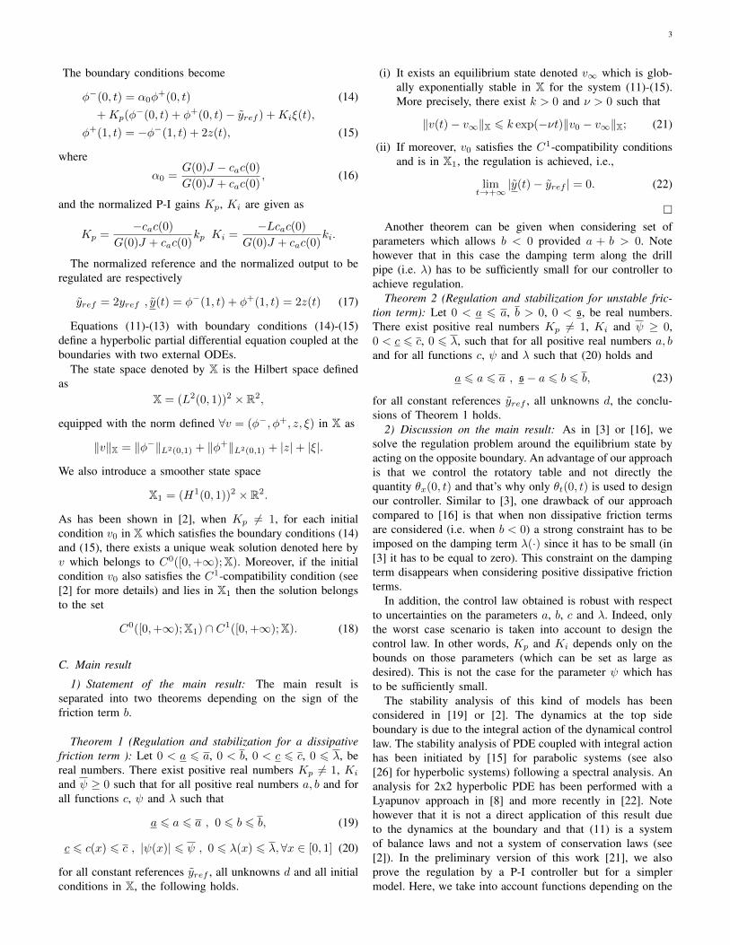
The friction β(x) models both possible rubbing between thedrill pipe and the drill holes and constant dynamic friction. Thefunction G(x) is supposed to be equal to G0 at x = 0 anddecreases along the drill pipe as the temperature and pressureincrease. Figure 1 depicts the shape of those functions. In theFigures 2 and 3, we compare the regulation action for different

Name Values Name ValuesG 79.6× 109 N.m−2 ρ 7850 kg.m−3

J 1.19× 10−5 m4 β 0.05 kg.m.s−1

ca 2000 N.m.s.rad−1 L 2000 mIb 311 kg.m−2 c 3184.3 m.s−1

cb 0.03 kg.s−1 T0 7500 N

TABLE IVALUES OF THE PHYSICAL COEFFICIENTS

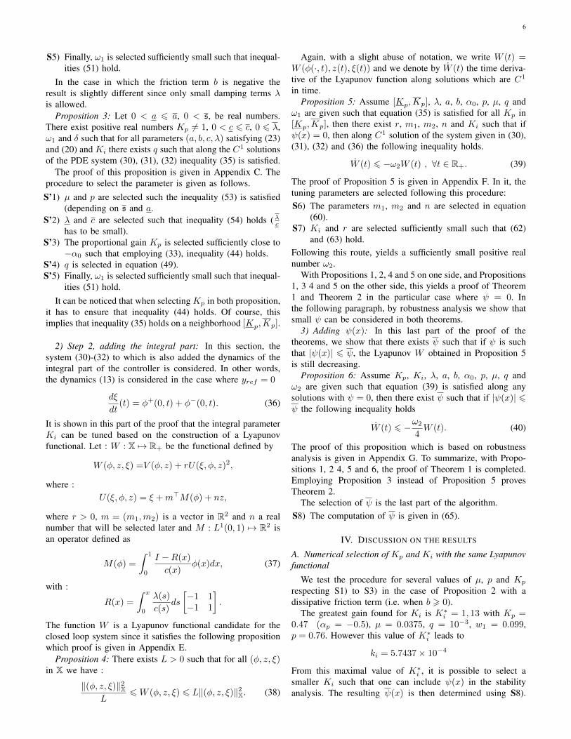
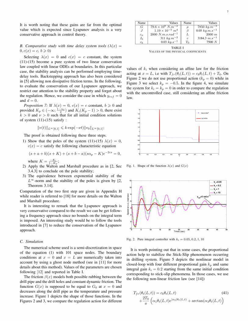
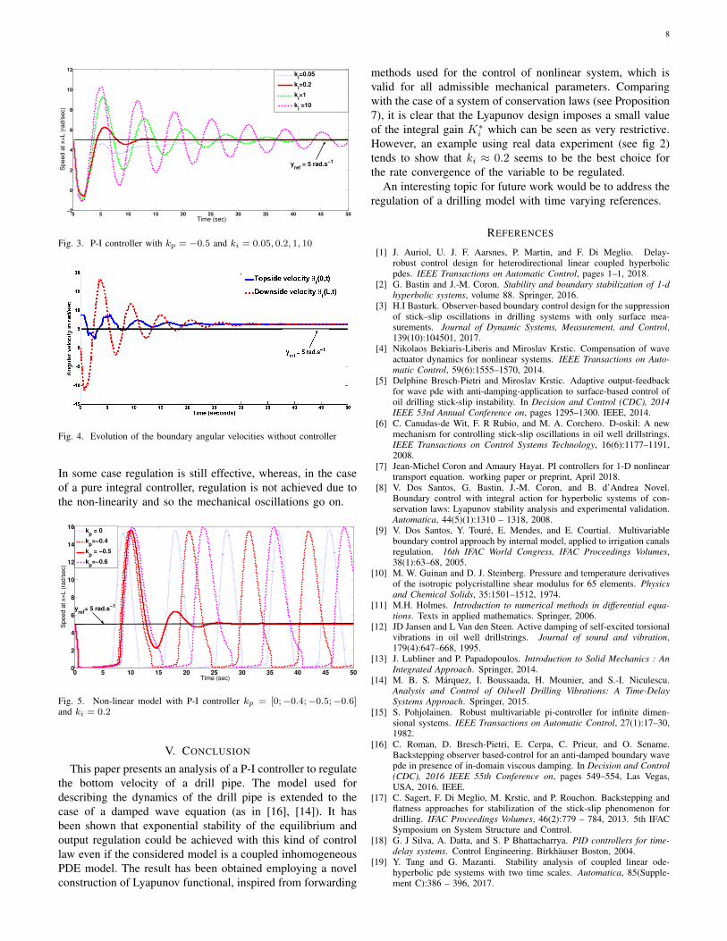
values of ki when considering an affine law for the frictionacting at x = L, i.e with Tfr(θt(L, t)) = cbθt(L, t) + T0. OnFigure 2 we do not use proportional action (kp = 0) while inFigure 3 we select kp = −0.5. In the figure 4, we simulatethe system for ki = kp = 0 in order to compare the regulationwith the uncontrolled case, still considering an affine frictionlaw.

0 0.1 0.2 0.3 0.4 0.5 0.6 0.7 0.8 0.9 10

0.2

0.4

0.6

0.8

1

1.2

1.4

1.6

1.8

2

x

G(x) in N/m2

λ(x) in N.s

Fig. 1. Shape of the function λ(x) and G(x)

0 5 10 15 20 25 30 35 40 45 50−2

0

2

4

6

8

10

12

Times (sec)

Sp

ee

d a

t x=

L (

rad

/sec)

k

i =0.05

ki = 0.2

ki = 1

ki = 10

yref

=5 rad.s−1

Fig. 2. Pure integral controller with ki = 0.05, 0.2, 1, 10

It is worth pointing out that in some cases, the proportionalaction help to stabilize the Stick-Slip phenomenon occurringin drilling system. Figure 5 depicts the nonlinear model inclosed-loop with four different proportional gain kp and sameintegral gain ki = 0.2 starting from the same initial conditioncorresponding to stick-slip phenomena. In those cases, we usethe following non-linear friction law (see [14])

Tfr(θt(L, t)) = cbθt(L, t) (41)

+2T0π

(α1θt(L, t)e

|α2|θt(L,t) + arctan(α3θt(L, t))

8

0 5 10 15 20 25 30 35 40 45 50−2

0

2

4

6

8

10

12

Time (sec)

Sp

ee

d a

t x=

L (

rad

/se

c)

ki=0.05

ki=0.2

ki=1

ki =10

yref

= 5 rad.s−1

Fig. 3. P-I controller with kp = −0.5 and ki = 0.05, 0.2, 1, 10

Fig. 4. Evolution of the boundary angular velocities without controller

In some case regulation is still effective, whereas, in the caseof a pure integral controller, regulation is not achieved due tothe non-linearity and so the mechanical oscillations go on.

0 5 10 15 20 25 30 35 40 45 500

2

4

6

8

10

12

14

16

Time (sec)

Spe

ed

at x=

L (

rad/s

ec)

kp = 0

kp=−0.4

kp = −0.5

kp=−0.6

yref

= 5 rad.s−1

Fig. 5. Non-linear model with P-I controller kp = [0;−0.4;−0.5;−0.6]and ki = 0.2

V. CONCLUSION

This paper presents an analysis of a P-I controller to regulatethe bottom velocity of a drill pipe. The model used fordescribing the dynamics of the drill pipe is extended to thecase of a damped wave equation (as in [16], [14]). It hasbeen shown that exponential stability of the equilibrium andoutput regulation could be achieved with this kind of controllaw even if the considered model is a coupled inhomogeneousPDE model. The result has been obtained employing a novelconstruction of Lyapunov functional, inspired from forwarding

methods used for the control of nonlinear system, which isvalid for all admissible mechanical parameters. Comparingwith the case of a system of conservation laws (see Proposition7), it is clear that the Lyapunov design imposes a small valueof the integral gain K∗i which can be seen as very restrictive.However, an example using real data experiment (see fig 2)tends to show that ki ≈ 0.2 seems to be the best choice forthe rate convergence of the variable to be regulated.

An interesting topic for future work would be to address theregulation of a drilling model with time varying references.

REFERENCES

[1] J. Auriol, U. J. F. Aarsnes, P. Martin, and F. Di Meglio. Delay-robust control design for heterodirectional linear coupled hyperbolicpdes. IEEE Transactions on Automatic Control, pages 1–1, 2018.

[2] G. Bastin and J.-M. Coron. Stability and boundary stabilization of 1-dhyperbolic systems, volume 88. Springer, 2016.

[3] H.I Basturk. Observer-based boundary control design for the suppressionof stick–slip oscillations in drilling systems with only surface mea-surements. Journal of Dynamic Systems, Measurement, and Control,139(10):104501, 2017.

[4] Nikolaos Bekiaris-Liberis and Miroslav Krstic. Compensation of waveactuator dynamics for nonlinear systems. IEEE Transactions on Auto-matic Control, 59(6):1555–1570, 2014.

[5] Delphine Bresch-Pietri and Miroslav Krstic. Adaptive output-feedbackfor wave pde with anti-damping-application to surface-based control ofoil drilling stick-slip instability. In Decision and Control (CDC), 2014IEEE 53rd Annual Conference on, pages 1295–1300. IEEE, 2014.

[6] C. Canudas-de Wit, F. R Rubio, and M. A. Corchero. D-oskil: A newmechanism for controlling stick-slip oscillations in oil well drillstrings.IEEE Transactions on Control Systems Technology, 16(6):1177–1191,2008.

[7] Jean-Michel Coron and Amaury Hayat. PI controllers for 1-D nonlineartransport equation. working paper or preprint, April 2018.

[8] V. Dos Santos, G. Bastin, J.-M. Coron, and B. d’Andrea Novel.Boundary control with integral action for hyperbolic systems of con-servation laws: Lyapunov stability analysis and experimental validation.Automatica, 44(5)(1):1310 – 1318, 2008.

[9] V. Dos Santos, Y. Toure, E. Mendes, and E. Courtial. Multivariableboundary control approach by internal model, applied to irrigation canalsregulation. 16th IFAC World Congress, IFAC Proceedings Volumes,38(1):63–68, 2005.

[10] M. W. Guinan and D. J. Steinberg. Pressure and temperature derivativesof the isotropic polycristalline shear modulus for 65 elements. Physicsand Chemical Solids, 35:1501–1512, 1974.

[11] M.H. Holmes. Introduction to numerical methods in differential equa-tions. Texts in applied mathematics. Springer, 2006.

[12] JD Jansen and L Van den Steen. Active damping of self-excited torsionalvibrations in oil well drillstrings. Journal of sound and vibration,179(4):647–668, 1995.

[13] J. Lubliner and P. Papadopoulos. Introduction to Solid Mechanics : AnIntegrated Approach. Springer, 2014.

[14] M. B. S. Marquez, I. Boussaada, H. Mounier, and S.-I. Niculescu.Analysis and Control of Oilwell Drilling Vibrations: A Time-DelaySystems Approach. Springer, 2015.

[15] S. Pohjolainen. Robust multivariable pi-controller for infinite dimen-sional systems. IEEE Transactions on Automatic Control, 27(1):17–30,1982.

[16] C. Roman, D. Bresch-Pietri, E. Cerpa, C. Prieur, and O. Sename.Backstepping observer based-control for an anti-damped boundary wavepde in presence of in-domain viscous damping. In Decision and Control(CDC), 2016 IEEE 55th Conference on, pages 549–554, Las Vegas,USA, 2016. IEEE.

[17] C. Sagert, F. Di Meglio, M. Krstic, and P. Rouchon. Backstepping andflatness approaches for stabilization of the stick-slip phenomenon fordrilling. IFAC Proceedings Volumes, 46(2):779 – 784, 2013. 5th IFACSymposium on System Structure and Control.

[18] G. J Silva, A. Datta, and S. P Bhattacharrya. PID controllers for time-delay systems. Control Engineering. Birkhauser Boston, 2004.

[19] Y. Tang and G. Mazanti. Stability analysis of coupled linear ode-hyperbolic pde systems with two time scales. Automatica, 85(Supple-ment C):386 – 396, 2017.

9

[20] A. Terrand-Jeanne and V. Dos Santos Martins. Modelings approaches forstick-slip phenomena in drilling. volume 49, pages 118–123, Bertinoro,Italy, 2016. Elsevier.

[21] A. Terrand-Jeanne, V. Dos Santos Martins, and V. Andrieu. Regulationof the downside angular velocity of a drilling string with a p-i controller.In Proceedings of European Control Conference, Limassol, Cyprus,2018.

[22] N.-T. Trinh, V. Andrieu, and C.-Z. Xu. Multivariable pi controller designfor 2× 2 systems governed by hyperbolic partial differential equationswith lyapunov techniques. In Decision and Control (CDC), 2016 IEEE55th Conference on, pages 5654–5659, Las Vegas, USA, 2016. IEEE.

[23] N.-T. Trinh, V. Andrieu, and C.-Z. Xu. Design of integral controllersfor nonlinear systems governed by scalar hyperbolic partial differentialequations. IEEE Transactions on Automatic Control, 2017.

[24] Ngoc-Tu Trinh, Vincent Andrieu, and Cheng-Zhong Xu. Output reg-ulation for a cascaded network of 2× 2 hyperbolic systems with picontroller. Automatica, 91:270–278, 2018.

[25] C.-Z. Xu and H. Jerbi. A robust pi-controller for infinite-dimensionalsystems. International Journal of Control, 61(1):33–45, 1995.

[26] C.-Z. Xu and G. Sallet. Multivariable boundary pi control and regulationof a fluid flow system. Mathematical Control and Related Fields,4(4):501–520, 2014.

APPENDIX

A. Modeling

In this subsection some explanation is given on the wayequation (1) is obtained to model the drill pipe dynamics.There exist several approaches to model the behavior ofmechanical deformations along the drill pipe in order tosynthesize a control policy. Early studies have consideredlumped parameter models of two or more states (see [12],[6]). If these models allow a wide choice of control strategies,they cannot take into account all possible vibration modes (see[20]). However, it is well known (see for instance [13, Chap 7])that when studying an infinitesimal slice of pipe with constantgeometry and properties, it is possible to express the torque(in N.m) induced by an angular deformation as

T (x, t) = GJθx(x, t).

The considered model has to take into account space varyingmechanical parameters and an external damping force actingalong the drill pipe. Consider an infinitesimal slice of pipebetween coordinates x and x + dx. The mechanical powerbalance into this slice yields

d

dtEc(x, t) = Pint + Pext.

Meaning that the variation of kinetic energy correspond tothe sum of intern and extern power. If one supposes that theHookes modulus may depends on the depth (and so on thetemperature and pressure along the drill hole [10]), the internalpower (in Watts) due to traveling torsion is written

Pint = Pin − Pout = (T (x, t)− T (x+ dx, t))θt(x, t)

= (G(x)θx(x, t)−G(x+ dx)θx(x+ dx, t)) Jθt(x, t)

The distributed damping implies :

Pext = −2πrσ(x)θ2t (x, t)dx in Watts

where σ(x) in N.s.m−1 refers to a surface friction coefficient,and the kinetic energy of this slice of pipe

Ec(x, t) = ρJθ2t (x, t)dx in Joules

So, considering the approximation

G(x)θx(x, .)−G(x+ dx)θx(x+ dx, .)

dx≈ ∂x (G(x)Jθx(x, .))

it yields that

θtt(x, t) =∂∂x (G(x)θx(x, t))

ρ− β(x)θt(x, t)

with β(x) = 2πrσ(x)ρJ .

Variables employed are summarized in Table I.

B. Proof of Proposition 2

The time derivative of V satisfies

V (t) = −w0(t)TPw0(t)− w1(t)TMw1(t)

−∫ 1

0

φ(x, t)TNφ(x, t)dx,

where

w0(t) =(φ+(0, t) Kiξ(t)

)T, w1(t) =

(φ−(1, t) z(t)

)T,

and :

M =

[e−µ − peµ 2peµ − aq2peµ − aq 2(a+ b)q − 4peµ

],

N =

[(2λ(x)c(x) + µ)e−µx λ(x)

c(x) (e−µx + peµx)λ(x)c(x) (e−µx + peµx) p

(2λ(x)c(x) + µ

)eµx

],

P =

[p− α2

p − αp(1−Kp)

− αp(1−Kp) − 1

(1−Kp)2

],

In the proof, the matrices M, N and P are consideredseparately.The matrix N : Note that

det(N (x)) = p

(2λ(x)

c(x)+ µ

)2

−(λ(x)

c(x)

(e−µx + peµx

))2

= F (p, µ, x)

[√p

(2λ(x)

c(x)+ µ

)+λ(x)

c(x)

(e−µx + peµx

)].

where

F (p, µ, x) =√p

(2λ(x)

c(x)+ µ

)− λ(x)

c(x)

(e−µx + peµx

).

(42)Hence, with Lemma 1 in Appendix D, there exist p and µ(depending on λ and c) such that

0 < p < e−2µ , (43)

and F (p, µ, x) > 0. So, N > 0.The matrix P : We pick Kp in (33) such that

p− α2p > 0. (44)

Then there exists a positive real number δ such that

−w0(t)TPw0(t) 6 δ|Kiξ(t)|2.

The matrix M : With (43), M > 0 if and only if

f(q) > 0 (45)

10

where :

f(q) = (e−µ − peµ)q(2(a+ b)− 4peµ)− (2peµ − aq)2

= −a′q2 + b′q − c′,

and a′, b′ and c′ are positives real numbers given as :

a′ = a2

b′ = (e−µ − peµ)2(a+ b) + 4paeµ

c′ = (e−µ − peµ)4peµ + 4p2e2µ = 4p

This function f(q) is a second order polynomial, whosemaximum is reached for q = b′

2a′ . Note that, f( 2b′

2a′ ) is strictlypositive if and only if

b′2 − 4a′c′ = (b′ − 2√a′c′)(b′ + 2

√a′c′) > 0. (46)

Since a′, b′ and c′ are positives, it remains to verify that b′ −2√a′c′ is positive. Keeping in mind that with (43), (e−µ −

peµ) > 0, it yields

b′ − 2√a′c′

(e−µ − peµ)= 2(a+ b)−

4a(√p− peµ)

e−µ − peµ(47)

= 2a

(1−

2√p

e−µ +√p

)+ 2b. (48)

Since 2√p

e−µ+√p < 1, it yields f( 2b′

2a′ ) > 0,consequently, we setas a function of (a, b) as

q =2b′

2a′=

(e−µ − peµ)2(a+ b) + 4paeµ

2a2, (49)

and M > 0.Conclusion : Consequently,

M > 0, N (x) > 0 , ∀x ∈ [0, 1], (50)

then, employing the fact that N is continuous, q is a continu-ous function of a and b (which belong to a compact set) andc is upper bounded, there exists ω1 in R+ (depending on a,a, and b) such that for all a, b these matrix inequalities

M > ω1qI , N (x) >ω1

c(x)

[1 00 p

], (51)

are satisfied. This implies that (35) holds.

C. Proof of Proposition 3

The proof follows mainly the same lines as the one ofProposition 2. The only difference comes from the analysisof the matrices M and P .The matrix M : Following the proof of Proposition 2 weconsider the case in which (43) holds. In that case, inequality(47) satisfies

b′ − 2√a′c′

(e−µ − peµ)= 2(a+ b)− 4a

√p

e−µ +√p. (52)

Picking p and µ such that

√p

2a− s

s< e−µ, (53)

yields√pa−ba+b < e−µ for all (a, b) satisfying (23). Conse-

quently 2√p

e−µ+√p < a+b

a and b′ − 2√a′c′ > 0 for all (a, b)

satisfying (23). It yields with q defined in (49) that M > 0.The matrix N : Note that the function F defined in (42)satisfies for all x in [0, 1] :

F (p, µ, x) > 2√pµ− λ

c(2√p+ 1 + peµ) .

Hence, selecting λc such that

λ

c<

2√pµ

2√p+ 1 + peµ

, (54)

yields N (x) > 0 for all x in [0, 1] and functions λ andc satisfying (20). The rest of the proof follows the one ofProposition 2.

D. Technical Lemmas

Lemma 1: Consider the mapping (p, µ, x) ∈ R+ × R+ ×[0, 1]→ R given by

F (p, µ, x) =√p

(2λ(x)

c(x)+ µ

)− λ(x)

c(x)

(e−µx + peµx

),

where0 6 λ(x) 6 λ , 0 < c 6 c(x).

Then, for all µ such that

µ > 0 ,e−µ

µ> 5

λ

c, (55)

there exists p such that

e−2µ > p > max C1(µ), C2(µ), C3(µ) , (56)

where Ci, i = 1, 2, 3 are given as

C1(µ) =

(4

5

)2

e−2µ,

C2(µ) = max

e−µ − c

λ

e−µ

10µ, 0

2

,

C3(µ) = e−2µ max

1− c

5λµ, 0

.

Moreover, for such couple (µ, p) and for all x in [0, 1]

F (p, µ, x) >e−µµ

5. (57)

Proof: Consider the function G : R+×[0, 1]→ R definedas

G(µ, x) = eµF (e−2µ, µ, x)− µ

= 2λ(x)

c(x)− λ(x)

c(x)

(eµ(1−x) + eµ(x−1)

)=λ(x)

c(x)

(2− eµ(1−x) − eµ(x−1)

).

Note that G(0, x) = 0 and moreover

Gµ(µ, x) =λ(x)

c(x)

(−(1− x)eµ(1−x) − (x− 1)eµ(x−1)

)which gives Gµ(0, x) = 0. Also,

Gµµ(µ, x) = −(1− x)2λ(x)

c(x)

(eµ(1−x) + eµ(x−1)

).

11

This implies for all µ ≥ 0 and all x in [0, 1]

|Gµµ(µ, x)| ≤ 2λ

ceµ.

Since,

G(µ, x) =

∫ µ

0

∫ r

0

Gµµ(s, x)dsdr ,

consequently, this yields for all µ ≥ 0 and all x ∈ [0, 1]

|G(µ, x)| 6∫ µ

0

∫ r

0

|Gµµ(s, x)| dsdr 6 λ

ceµµ2. (58)

On one hand, it yields

F (p, µ, x) = (√p− e−µ)

(2λ(x)

c(x)+ µ

)− e−µ

λ(x)

c(x)

(eµ(1−x) + eµ(x−1)

)+ e−µ

(2λ(x)

c(x)+ µ

)− λ(x)

c(x)(p− e−2µ)eµx

= (√p− e−µ)

(2λ(x)

c(x)+ µ

)− λ(x)

c(x)(p− e−2µ)eµx + e−µG(µ, x) + e−µµ.

Hence, with (58), this implies that

F (p, µ, x) > e−µµ− |√p− e−µ|(

2λ

c+ µ

)− λ

c|p− e−2µ|eµ − µ2λ

c

> e−µµ− |√p− e−µ|µ

− λ

c(2|√p− e−µ|+ |p− e−2µ|eµ + µ2).

On the other hand, (55) gives,

λ

cµ2 <

e−µµ

5. (59)

Moreover if e−2µ > p > C1(µ), it yields

|e−µ −√p| = e−µ −√p 6 e−µ

5.

Moreover, if e−2µ > p > C2(µ), it implies

2λ

c|e−µ −√p| = 2

λ

c(e−µ −√p) 6 e−µµ

5.

Finally, if e−2µ > p > C3(µ), it yields

λ

c|e−2µ − p|eµ =

λ

c(e−2µ − p)eµ 6 e−µµ

5.

Consequently, this implies that (57) holds.

E. Proof of Proposition 4

First of all, note that with the definition of the function Vin (34), and since p < 1, one gets

V (φ, z) 6 q|z|2 +1

c‖φ−‖2L2(0,1) +

peµ

c‖φ+‖2L2(0,1)

6 L1

(|z|+ ‖φ−‖L2(0,1) + ‖φ+‖L2(0,1)

)2,

where L1 = maxq, 1c ,

peµ

c

. Also,

V (φ, z) > q|z|2 +e−µ

c‖φ−‖2L2(0,1) +

p

c‖φ+‖2L2(0,1)

> L2

(|z|+ ‖φ−‖L2(0,1) + ‖φ+‖L2(0,1)

)2,

where L2 = minq3 ,

e−µ

3c ,p3c

. Moreover,

U(ξ, φ, z) 6 |ξ|+ |n||z|

+ |m|c+ 2λ

c2(‖φ−‖L2(0,1) + ‖φ+‖L2(0,1)

)6 L3‖(φ, z, ξ)‖X.

where L3 = max

1, |m| c+2λc2 , |n|

. Finally note that

U(ξ, φ, z) = ξ + Z(φ, z),

where

Z(φ, z) = mTM(φ) + nz 6√L3V (φ, z).

where L3 is a positive real number. Hence, it yields

U(ξ, φ, z)2 > |ξ|2 + Z(φ, z)2 − 2|ξ||Z(φ, z)|.

By completing the square this implies for all 0 < ` < 1

U(ξ, φ, z)2 > |ξ|2(1− `)−(

1

`− 1

)|Z(φ, z)|2

> |ξ|2(1− `)−(

1

`− 1

)L3V (φ, z).

Finally, this yields setting ` sufficiently closed to 1 and apositive real number L4 such that,

W (ξ, φ, z) > r|ξ|2(1− `) +

(1− r

(1

`− 1

))L3V (φ, z)

61

L4‖(φ, z, ξ)‖2X.

Hence, setting L > maxL2, L3, L4, the result is obtained.

F. Proof of Proposition 5

Let Kp be in [Kp,Kp]. First of all

R(x)

[1 11 1

]= 0.

Hence, we get the property

M(t) =

∫ 1

0

I −R(x)

c(x)φt(x, t)dx

=

∫ 1

0

(I −R(x))

[−1 00 1

]φx(x, t)

− λ(x)

c(x)

[1 11 1

]φ(x, t)dx.

12

Note that

Rx(x)

[−1 00 1

]=λ(x)

c(x)

[1 11 1

].

Consequently, with an integration by parts, it yields

M(t) = (I −R(1))

[−1 00 1

]φ(1, t)−

[−1 00 1

]φ(0, t)

=

[−1− ζ −ζ−ζ 1− ζ

]φ(1, t)−

[−1 00 1

]φ(0, t),

where

ζ =

∫ 1

0

λ(x)

c(x)dx.

Consequently,

U(t) = φ−(0, t) + φ+(0, t)− n(a+ b)z(t) + naφ−(1, t)

+m1

(φ−(0, t)− (1 + ζ)φ−(1, t)− ζφ+(1, t)

)+m2

(−λ

2φ−(1, t) + (1− ζ)φ+(1, t)− φ+(0, t)

)Employing the boundary conditions (32) and αp defined in(33), it yields

U(t) = φ−(1, t)

(an−m1 (1 + ζ)−m2ζ −

n(a+ b)

2

)+ φ+(1, t)

(m2 (1− ζ)−m1ζ −

n(a+ b)

2

)+ φ+(0, t)(αp + 1 +m1αp −m2)

+ ξ(t)Ki

1−Kp(1 +m1) .

Our aim is now to solve in m1, m2 and n the system−1− ζ −ζ a−b2

−ζ 1− ζ −a+b2αp −1 0

m1

m2

n

=

00

−αp − 1

It is possible with

n =2(αp + 1)

a (1− αp + 2ζ(1 + αp)) + (αp + 1)b,

m2 =+2aαp

a (1− αp + 2ζ(1 + αp)) + (αp + 1)b+ 1

m1 =2a

a (1− αp + 2ζ(1 + αp)) + (αp + 1)b− 1.

(60)

These values are defined for almost all αp hence for almostall Kp in [Kp,Kp]. In that case, it yields

U(t) = ξ(t)Ki

1−Kp(1 +m1)

So we select Ki such that Ki1−Kp (1 +m1) < 0.

Hence, we get

2U(t)U(t)

|Ki|6 −ξ(t)2

∣∣∣∣1 +m1

1−Kp

∣∣∣∣+ ξ(t)m>M(t) + ξ(t)nz

6 −c1ξ(t)2 + c2V (t),

where c1 and c2 are obtained by applying the Cauchy Schwartzinequality and by completing the square. Finally, this with (35)yield

W (t) 6 (c2r|Ki| − ω1)V (t) + (δ − rc1)|Ki|ξ(t)2. (61)

So, we select0 < |Ki| <

ω1c1δc2

. (62)

Hence, we can choose r such thatδ

c1< r <

ω1

c2|Ki|. (63)

This implies the existence of a positive real number ω2 suchthat equation (39) holds.

G. Proof of Proposition 6

Since inequality (39) is satisfied by assumption and exhibit-ing all the terms in which ψ shows up in the time derivativeof the Lyapunov function, it yields along the solution of thesystem :

W (t) 6 −ω2W (t)

+2

∫ 1

0

ψ(x)

c(x)2φ(x, t)>

[e−µx 0

0 peµx

] [−1 1−1 1

]φ(x, t)dx

+2rU(t)m>M

(ψ(·)c(·)

[−1 1−1 1

]φ(·, t)

),

where M is the bounded linear operator defined in (37).Note that

2

∫ 1

0

ψ(x)

c(x)2φ(x, t)>

[e−µx 0

0 peµx

] [−1 1−1 1

]φ(x, t)dx

6 r1ψV (t) 6 r1ψW (t),

with r1 is a positive real number (depending on c, p and µ)such that for all x in [0, 1]

1

c(x)

[−2e−µx e−µx − peµx

e−µx − peµx 2peµx

]6 r1

[e−µx 0

0 peµx

].

Also, note that since rU(t)2 6W (t), it yields

2rU(t)m>M

(ψ(·)c(·)

[−1 1−1 1

]φ(·)

)6 r2ψ

√W (t) ‖φ(·, t)‖(L1(0,1))2 , (64)

where

r2 = 2√r|m|‖M‖(L1(0,1))2;R2)

1

c

∥∥∥∥[−1 1−1 1

]∥∥∥∥ .With Holder inequality, and Proposition 4 it yields a positivereal number r3 such that

r2‖φ(·, t)‖(L1(0,1))2 6 r3√W (t)

In conclusion,

W (t) 6 (−ω2 + (r1 + r3)ψ)W (t)

Hence, withψ =

ω2

2(r1 + r3), (65)

equation (40) holds.

13

H. Proof of Proposition 7

Consider the system of equations (11)-(15) with λ(x) =ψ(x) = 0 and c(x) = c constant and b > 0. Employing theLaplace transform the following equalities for the dynamicsmay be obtained

sξ(s) = φ−(0, s) + φ+(0, s)

z(s) =a

s+ a+ bφ−(1, s)

φ−(1, s) = φ−(0, s)e−cs, φ+(0, s) = φ−(1, s)e−cs

At x = 0 the boundary condition (14) imposes:

s(1−Kp)φ−(0, s) =

sαp(1−Kp)φ+(0, s) +Ki(φ

−(0, s) + φ+(0, s)),

which gives

φ−(0, s) =sαp(1−Kp) +Ki

s(1−Kp)−Kiφ+(0, s)

while at x = 1, conditions (15) becomes:

φ+(1, s) = −φ−(1, s) +2a

s+ a+ bφ−(1, s)

φ+(1, s) =a− s− bs+ a+ b

φ−(1, s)

=(a− s− b)(s+ a+ b)

(sαp(1−Kp) +Ki)

(s(1−Kp)−Ki)e−2csφ+(1, s)

Thus, we obtain a characteristic equation of the form

(s+a+b)(s− Ki

(1−Kp))+(s+b−a)(sαp+

Ki

(1−Kp))e−2cs = 0

Set K = − Ki1−Kp to get the following characteristic equation

(s+ a+ b)(s+K) + (s+ b− a)(sαp −K))e−2cs = 0 (66)

We follow the Walton and Marshall procedure as is it used in[2] and described in [18]First step : the roots of (66) are examined with c = 0In this case, one looks for the roots of

(1 + αp)s2 + (a+ b+ αp(b− a))s+ 2aK = 0

which are

s1 = −a(1− αp) + b(1 + αp)

2(1 + αp)

+

√(a(1− αp) + b(1 + αp))2 − 8aK(1 + αp)

2(1 + αp)

s1 = −a(1− αp) + b(1 + αp)

2(1 + αp)

−√

(a(1− αp) + b(1 + αp))2 − 8aK(1 + αp)

2(1 + αp)

Provided that

sgn(Ki) = sgn(Kp − 1), Ki 6= 0

the system poles have strictly negative real part for c = 0.

Second step : We compute the polynomial in w2 :

W (w2) , d(jw)d(−jw)− n(jw)n(−jw)

withd(x) = (x+ a+ b)(x+K) andn(x) = (x+ b− a)(xαp − K) then,

W (X) = (X + (a+ b)2)(X +K2)

−(X + (b− a)2)(α2pX +K2)

= (1− α2p)X

2 +((a+ b)2 − α2

p(b− a)2)X + 4abK2

where X = w2. Notes that Kp ∈] − ∞; 1−α0

2 [⇒ |αp| < 1.It implies that the sign of the polynomial W is positive forlarge X . We can deduce that the poles of the system havestrictly negative real parts for sufficiently small value of c.

Third step : Computing the roots of W (X)We obtain

X1 =−((a2 + b2)(1− α2

p) + 2ab(1 + α2p))

2(1− α2

p

) +√((a2 + b2)(1− α2

p) + 2ab(1 + α2p))2 − 16abK2

(1− α2

p

)2(1− α2

p

)X2 =

−((a2 + b2)(1− α2

p) + 2ab(1 + α2p))

2(1− α2

p

) −√((a2 + b2)(1− α2

p) + 2ab(1 + α2p))2 − 16abK2

(1− α2

p

)2(1− α2

p

)which have strictly negative real parts since

((a2 + b2)(1−α2p) + 2ab(1−α2

p)) > 0, abK2(1− α2

p

)> 0

for all positive parameters.After these three steps, we can conclude that for every negativevalue of Ki, the poles of the system governed by (11)-(15) inthe special case where λ(x) = ψ(x) = 0 and c(x) = c arestable whatever the length L or the velocity c.

Alexandre Terrand-Jeanne graduated in electricalengineering from ENS Cachan, France, in 2013.After one year in the robotic laboratory ”CentroE.Piaggio” in Pisa, Italy, he is currently a doctoralstudent in LAGEP, university of Lyon 1. His PhDtopic concerns the stability analysis and controllaws design for systems involving hyperbolic partialdifferential equations coupled with nonlinear ordi-nary differential equations. This work is under thesupervision of V. Dos Santos Martins, V. Andrieuand M. Tayakout-Fayolle.

14

Vincent Andrieu graduated in applied mathemat-ics from INSA de Rouen, France, in 2001. Af-ter working in ONERA (French aerospace researchcompany), he obtained a PhD degree from Ecoledes Mines de Paris in 2005. In 2006, he had a re-search appointment at the Control and Power Group,Dept. EEE, Imperial College London. In 2008, hejoined the CNRS-LAAS lab in Toulouse, France,as a CNRS-charge de recherche. Since 2010, hehas been working in LAGEP-CNRS, Universite deLyon 1, France. In 2014, he joined the functional

analysis group from Bergische Universitat Wuppertal in Germany, for twosabbatical years. His main research interests are in the feedback stabilizationof controlled dynamical nonlinear systems and state estimation problems. Heis also interested in practical application of these theoretical problems, andespecially in the field of aeronautics and chemical engineering.

Melaz Tayakout-Fayolle is a Full Professor with theLAGEP (Laboratoire dAutomatique et de GEnie desProcedes) of University of Lyon 1. She received herBSc in Physics and Chemistry and MSc in IndustrialChemistry from the University of Marseille. HerPh.D. degree in Chemical Engineering was obtainedin 1991 from the University of Lyon. She stardedas an Associated Professor at LAGEP (LaboratoiredAutomatique et Genie des Procedes) of the Uni-versity of Lyon. Prior to joining IRCELYON asFull Professor, she worked three years as Research

Engineer for IFPEN Compagny. Since 1991, she has taught courses in chem-ical engineering, thermodynamics, mass transfer, dynamical modelling. Herresearch areas of interest include modelling of triphasic reactors: mass transfer,chemical kinetics of the complex matrix and thermodynamics, and designconcepts in reactors. The complex matrix concerns the heaviest fractions ofpetroleumin in hydroconversion and hydrocracking processes. Since 2014, sheis a consultant for the Total Company.

Valerie Dos Santos Martins graduated in Math-ematics from the University of Orleans, France in2001. She received the Ph.D degree in 2004 in Ap-plied Mathematics from the University of Orleans.After one year in the laboratory of MathematicsMAPMO in Orleans as ATER, she was post-doctin the laboratory CESAME/INMA of the UniversityCatholic of Louvain, Belgium. Currently, she is pro-fessor assistant in the laboratory LAGEP, Universityof Lyon 1. Her current research interests includenonlinear control theory, perturbations theory of

operators and semigroup, spectral theory and control of nonlinear partialdifferential equations.