regression models for lar generation - ucm · master in mathematical engineering regression models...

Master in Mathematical Engineering

Regression models for LAR Generation

VIII Modelling Week UCM

Daniel Becerra Clemares

Pedro García Segador

Álvaro Huete Oliva

Yakelin Lizbeth Romero Triviños

INDEX

1. Introduction ................................................................................................. 1

2. Description of the first model ...................................................................... 4

2.1 Regression techniques.......................................................................... 5

2.2 Polar regression model validation ........................................................ 7

2.3 Complete model and validation ........................................................... 8

2.4 First validation method ........................................................................ 8

2.5 Second validation method ................................................................... 9

3. Second regression technique. Non-parametric model ................................ 10

3.1 Matlab code ........................................................................................ 12

3.2 Results ................................................................................................. 15

3.3 The problem ........................................................................................ 16

4. Conclusions ................................................................................................... 18

VIII MODELLING WEEK UCM Master in Mathematical Engineering

1

1. INTRODUCTION

The problem approached during this Modelling Week, proposed by MBDA, consists on

designing a model to improve the accuracy of the LAR.The acronym LAR means Launch

Acceptability Region or Launch Acceptable Region. The term is applicable to bombs, rockets,

and missiles whether the weapon is designed to engage a target on the ground or in the air.

The LAR defines a region of conditions where a weapon can be successfully launched to reach

a specified target. In the case of a weapon released from an aircraft, these launch conditions

usually take into account variables like the range to the target, the speed and altitude of the

aircraft, and the capabilities of the weapon itself. The primary factors that typically limit the

launch envelope of a weapon are its kinematic performance and seeker capabilities.

Kinematic performance refers to the energy a weapon has during the course of its flight.

Missiles, for example, are equipped with jet or rocket propulsion systems that carry a limited

amount of fuel. Once this fuel supply is exhausted, the missile starts to slow down and lose

energy. This loss of energy gradually degrades the missile's ability to maintain altitude and

maneuver towards its target. Once sufficient energy is lost, the missile may not be able to

reach its target at all. Unpowered weapons like bombs are even more limited in kinematic

performance since the only energy the weapon has during its flight comes from the initial

momentum of being launched from a moving plane plus the acceleration due to gravity as it

falls to the ground. A careful management of a weapon's energy is a key factor in maximizing

its performance and is often the limiting factor on its launch region.

There are other weapons, however, that have the kinematic capability to travel much farther

than they can actually engage a target. These weapons are typically limited by the capabilities

of their seekers. A seeker gives a weapon the ability to see its target as it flies. Some seekers,

particularly those operating in optical or infrared wavelengths, are often limited in the distance

they are able to differentiate a target from its surroundings. A pilot may not be able to lock the

seeker onto a target until he is much closer to the target than the weapon is actually capable

of flying based purely on its kinematic performance. In this case, it is the seeker that limits the

maximum range at which the weapon can be launched.

Based upon these limitations, it is possible to construct a chart showing the region in which a

given weapon can reach a given target at a given location. This chart is called the Launch

Acceptability Region or LAR. The following picture shows a conceptual example of what a LAR

might look like for a weapon launched by an aircraft flying at a certain altitude, speed, and

heading at the time of release.

The usual approach is generates the Weapon Attainability Region (WAR) of the ammo and

after that generate the LAR.

The WAR is defined as the area that a weapon can reach given its kinematics characteristics

and the initial conditions, that means that is weapon dependant.

http://www.aerospaceweb.org/question/weapons/q0211.shtml


http://www.aerospaceweb.org/question/propulsion/q0033.shtml

http://www.aerospaceweb.org/question/propulsion/q0161.shtml



2

Figure1.Concept of a Launch Acceptable Region (LAR)

This type of scenario is often referred to as an off-axis or off-boresight launch. Such cases are

made possible by the fact that many seekers have gimbals that allow the weapon to see a

target that is not directly in front of it. If the gimbal limits are large enough, the weapon can

potentially be aimed towards and locked onto a target that is at a considerable angle off of the

aircraft's boresight. This capability gives a pilot the ability to launch towards targets off to his

or her side and reduce the danger posed by enemy defenses. In such a case, however, part of

the weapon's energy is used to turn it away from the flight path of the launch aircraft and

move in a crossrange direction towards the target. This loss of energy reduces the overall

performance of the weapon causing the launch region and maximum range to shrink.

Figure2. Example of LAR for a high off-boresight scenario

The above example illustrates such a case for a very high off-boresight scenario. In both this

example and the previous one, the launch aircraft is flying at the same speed, altitude, and

heading. Only its position relative to the target has changed. Since the aircraft is headed away

from the target in this example, however, the weapon is forced to make a very large turn away

from the aircraft's heading in order to move towards the target. This maneuver uses up much

of the weapon's kinematic energy resulting in a much smaller maximum range in this region of

the LAR compared to the previous example.


3

A further illustration of the importance of maneuvers in determining the size of the launch

region can be seen below. This example assumes the weapon is capable of flying along a flight

path that includes pre-programmed waypoints.

Figure3. Example of LAR for a weapon flying pre-planned waypoints

The WAR could be made by means of the simulation of the fly-out of a given weapon for each

launch and environmental conditions, and for each target point. This means that the in flight

simulation of the WAR is not possible. One solution is to simulate on ground all the possibilities

and load it into airborne equipment. The other is to prepare a model which generates it in

flight.

4a 4b

4c 4d


4

Figure4. Simulations of the weapon’s behavior on three spatials axes in a flight time of fifty

seconds. Acceleration (4a), altitude from ground (4b), flight speed (4c) and push (4d)

When the zone attainable by a weapon has been determined the LAR could be calculated to

indicate the platform operator where to steer the platform to engage the target. This is based

on the target speed and bearing. In zero wind conditions the LAR could be obtained from the

WAR by a rotation and an axis transformation. In case that the wind is non zero the two

surfaces have different shape.

The process could be summarized as follows:

1. A high fidelity simulation model is implemented for the weapon engagement.

2. Using Monte-Carlo runs a truth table for the WAR is generated based on the

parameters that will be included in the model. These data will be supplied by MBDA

based on the simulation of a generic system.

3. A regression technique is used to estimate a parametric model for the WAR, an

excursion could be a neural network.

4. The obtained WAR is transformed to obtain the LAR.

5. The parametric model is used to generate the in-flight prediction based on the real

data measured by the platform.

In this work, we will use the data from the truth table supplied by MBDA with zero wind

conditions.

2. DESCRIPTION OF THE FIRST MODEL

Some simplifications will be assumed such as fixedand disarmed target, alsowe will suppose

that there isno wind nor rain.

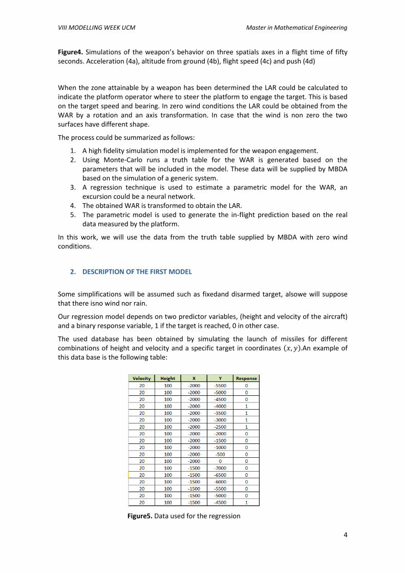
Our regression model depends on two predictor variables, (height and velocity of the aircraft)

and a binary response variable, 1 if the target is reached, 0 in other case.

The used database has been obtained by simulating the launch of missiles for different

combinations of height and velocity and a specific target in coordinates An example of

this data base is the following table:

Figure5. Data used for the regression


5

2.1 REGRESSION TECHNIQUES

The first regression technique is based on polar coordinates. The goal of the model is to obtain

a function that provides the WAR with the predictor variables as input data. Using the MBDA

database, the first step is to fix a certain height and velocity and plot the response variable

(WAR) in order to get an idea of the generic WAR shape.

Firstly, we take a for flight speed and for flight altitude and plot the response

variable values, the blue area represents the WAR and the red one represents the points

where the weapon fails his impact on target.

Figure5. Representation of WAR using simulated data. There is a blind angle behind the shape.

We can observe in Figure 5 that region obtained is approximately a cardioid, whose polar

equation is given by:

But this simple equation is not able to explain the full behavior of WAR, so we need to improve

it adding some terms in Föurier series form:

In this model, the predictor variable is angle, and the response variable is radius .

Regression curves for each value of flight altitude and flight speed fitting the simulated impact

points are calculated. Note that these regressions are linear regressions and the coefficients and can be easily calculated by using the analytical expression of least squares

to linear regressions.

In order to get a single radius for each value, we have to move the reference system

to another point different from .

The data provided from MBDA database are symmetric, therefore we only need to calculate

half regression curve and duplicate it. The following linear regression is solved for each of the

45 curves:

-8000 -6000 -4000 -2000 0 2000 4000 6000 8000 10000 12000-8000

-6000

-4000

-2000

0

2000

4000

6000

8000Weapon Attainability Region (WAR) with v=20 and h=100

X

Y


6

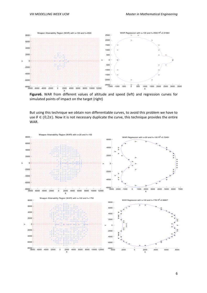
Figure6. WAR from different values of altitude and speed (left) and regression curves for

simulated points of impact on the target (right)

But using this technique we obtain non differentiable curves, to avoid this problem we have to

use . Now it is not necessary duplicate the curve, this technique provides the entire

WAR.

-8000 -6000 -4000 -2000 0 2000 4000 6000 8000 10000 12000-8000

-6000

-4000

-2000

0

2000

4000

6000


X

Y

-1500 -1000 -500 0 500 1000 1500 2000 2500 3000 3500-2500

-2000

-1500

-1000

-500

0

500

1000

1500

2000

2500WAR Regression with v=100 and h=4500 R2=0.91864

X

Y

-8000 -6000 -4000 -2000 0 2000 4000 6000 8000 10000 12000-8000

-6000

-4000

-2000

0

2000

4000

6000


X

Y

-3000 -2000 -1000 0 1000 2000 3000 4000 5000 6000 7000-6000

-4000

-2000

0

2000

4000


X

Y

-8000 -6000 -4000 -2000 0 2000 4000 6000 8000 10000 12000-8000

-6000

-4000

-2000

0

2000

4000

6000


X

Y

-4000 -2000 0 2000 4000 6000 8000-8000

-6000

-4000

-2000

0

2000

4000

6000


X

Y


7

Figure7. WAR from different pairs of altitude and speed (left) and regression curves for

simulated points of impact on the target (right) without non differentiable points

This way we obtain a more realistic WAR approach. Since we are working on a physical

problem, it is much easier to think about a regular region where missile can reach its targets.

We have used the Matlab function regression to get these curves (see Figure8).

Figure8. Code to do the polar regression

2.2 POLAR REGRESSION MODELS VALIDATION

In this section we are going to study the quality of the fittings performed with the last two

models. We call model 1 to the first model in which just half curve is fitted. This was the model

that shows non differentiable points. Model 2 refers to the model where the regression is

done with and provides regular curves.

For each combination of altitude and speed R squared statistic has been used as measure of

the fitting quality. R squared statistic is used to know the percentage of explained variance for

our model. Since our database has 45 different pairs of altitude and speed, we have 45

different fittings and 45 different R squared. By using model 1 and model 2 the obtained

results were really good. Only few curves were not fitted properly and almost all R squared

were above 85%. The following table shows how these regressions work for each model.

Figure9. R squared table for the two polar models

The curves in which the regression did not work well were the ones for which we have few

data to estimate the WAR.


8

2.3 COMPLETE MODEL AND VALIDATION

The goal of this section is to construct a model do not depends on speed and altitude. To get

this objective we are going to do other linear regression on the parameters obtained for each

curve. So we have a set of 45 observation for 5 different coefficients and . Now

we adjust a linear regression with the following features to each of these coefficients,

where is the velocity and the height of the aircraft. It is important to realize that the

monomials with variables and are essential to get the relationship between the two

variables in our set of data. We call this model the complete model because it does not

depends on the speed and altitude. This regression has an R squared of 80% for the whole data

set. After doing this regression only speed and altitude should be written in the obtained

expression to get a fitting curve for WAR region.

This kind of model is very useful to aircraft because they cannot waste technological sources

by using models in which lots of calculations are required.

Now we are going to provide two different methods to validate the complete model.

The code to do this regression is the following.

Figure10. Code to do the parameters regression

2.4 FIRST VALIDATION METHOD

The first method consist in dividing the database in two sets, a training set with the 80% and a

validation set with the 20% of the database. In the two set each pair of altitude and speed are

considered. The training set is used to construct the complete model and the validation set is

used measure the error. The error between this model and the real points is measured by

considering distances between points and model curve. The following table shows the quality

of the fittings.


9

Figure11. R squared table for the complete model

It is important to consider that the last regression was done with just 45 data. For this reason

the complete model cannot describe perfectly the behavior of every curve.

2.5 SECOND VALIDATION METHOD

This time the sensibility of the complete model parameters is tested. To do this the original

data are separated in two sets with different pairs of altitude and velocity. After this, two

complete models are constructed and the difference between the obtained parameters is

measured by the formula:

This formula measure how much the parameters change when we change the data used to

construct the model. This sensibility measure is near 1 when the parameters are completely

stable and lower when the stability is worse.

The sensibility measure obtained with the data provided by MBDA was .

Now we are going to see this comparison in a more graphical way.

-4000 -2000 0 2000 4000 6000 8000-8000

-6000

-4000

-2000

0

2000

4000

6000

8000

X

Y

WAR Regression with v=20 and h=100

Regression Model

Model 1

Model 2

WAR Frontier

-2000 -1000 0 1000 2000 3000 4000-3000

-2000

-1000

0

1000

2000

3000

X

Y


Regression Model

Model 1

Model 2

WAR Frontier


10

Figure12. Complete model curves for different pairs of altitude and speed

Here the blue curve is the regression curve obtained with the differentiable polar model. We

can think about this curve as the real WAR frontier. The red curve is the first complete model

constructed with half of pairs of altitude and speed and the green curve is the second

complete model. The distance between curves red and green tells us about the parameter

stability. We can see how in some cases the curves are very close to each other. That is a signal

of the parameter stability. Also the distance between each model and blue curve tells us about

the accuracy of the model. In some cases the complete models are not so close to the blue

line, that occurs because we are using very few data to construct the last regression (around

27 observations per model). With a bigger database the results will improve a lot.

3 SECOND REGRESSION TECHNIQUE. NON-PARAMETRIC MODEL

The second regression technique is the Projection Pursuit Regression. The main goal of this

technique is provide a response surface which will produce a good fit to the data based on a

distance criterion (squared-error). We will use just the coordinates X and Y as variables,

keeping a fixed initial velocity and height. A little summary of this method is:

• First step, initialize residuals.

• Second step, construct a smooth representation of the data.

• Third step, maximize the fraction of variance that can be explained by the smooth

representation.

• Fourth step, update the response function.

• Fifth step, update the residual.

• Sixth step, if the residuals are smaller than a threshold, stop. In other case, go to

second step.

This methodology can be summarized as follow in the next diagram:

-4000 -2000 0 2000 4000 6000 8000 10000-8000

-6000

-4000

-2000

0

2000

4000

6000

8000

X

YWAR Regression with v=100 and h=1750

Regression Model

Model 1

Model 2

WAR Frontier

-3000 -2000 -1000 0 1000 2000 3000 4000 5000 6000 7000-5000

-4000

-3000

-2000

-1000

0

1000

2000

3000

4000

5000

X

Y


Regression Model

Model 1

Model 2

WAR Frontier


11

Figure13. Projection Pursuit Regression workflow.

The final result of the non-parametric model will be a surface for each initial velocity and

height, where the Z coordinate will be a measurement of probability of reaching the target

depending on the X and Y coordinates in our data. The equation of the surface is:

∑

With X the variables vector ((X, Y) in our case) and a coefficient vector.

The regression stats with initial residuals equal to the response variable (the target): Then, it search for the next term of the model. It creates a linear combination of the

variables , with a coefficient vector of real numbers (the value of will be given in

the next step) and X the variables vector, and constructs a smooth representation of the

residuals.

We have to be careful in this step, because this notation is hiding some problems to deal with.

The new variable Z is a one-dimensional variable created with the two-dimensional variable X.

It means that, for a given value of , the variable Z must be sorted so as to represent the

function . But each of our variables X has an assigned target (in next iteration

residuals ) so this target must be sorted in the same way as Z. Then, will be a smooth

representation of a function which gives for each Zi his values (multiple values,

because Zi could be obtained by more of one Xi).


12

For example, if Zi has two zeros and five ones, could be the mean of this values. In our

case, the mean provides a graphic with a non-structured function, so we proposed a more

structured smooth function: .

In order to calculate the surface , the order of Z in each loop will be saved.

The method considers another function I(α) named the Figure of Merit which gives the fraction

of unexplained variance that will be explained by : ∑ ( ) ∑ ⁄

In this step the algorithm finds the coefficient vector that maximizes I(α).

Now, the corresponding is a smooth function of variance unexplained in the loop

number m so a linear regression in these data will provide a function with the information

unexplained yet. The coefficients of the regressions will be saved for the calculus of .

Finally, if the Figure of Merit is smaller than a threshold, stop. Otherwise, update the current

residuals:

Outside the regression algorithm, the response surface will be calculated adding the

coefficient of each regression of the smooth function. Reminding the equation:

∑

The corresponding regression of will be added considering the same order that

the 2-dimensional variable X (we have seen that has a different order in each loop in

order to calculate the smooth function), so will be sorted as in the data for each

m.

3.1 MATLAB CODE

In our case, the data will be represented in three columns: first one, the X coordinate; second

one, the Y coordinate; third one, the target (0 if it was not reached, 1 if it was reached).

The function in Matlab that represents this non-parametric regression technique provides:

The alpha vector which maximizes the Figure of Merit in each loop.

The matrix with the regression coefficient of the smooth function in each loop

The matrix with the Z vector of each loop.

The matrix of the order of Z in each loop.

To do this, the function ask for:

The matrix with the two first columns of X coordinate and Y coordinate and the target.

The threshold.

First of all, initialize residuals, initialize the tolerance (value of figure of merit) and normalize

the data in order to have all the data between 0 and 1 (Figure 14):


13

Figure14. Matlab function of Projection Pursuit Regression. Initializing variables.

After that, the loop starts. Firstly, alpha vector is calculated. The Figure of Merit is multiplied

by -1 so as to calculate the alpha vector which minimizes this.

Once calculated the alpha vector, the tolerance is updated as the value of the Figure of Merit

(minus the value of the minus Figure of Merit) in the vector alpha estimated before, and

calculate the Z vector of points sorted as usually (Figure 15):

Figure15. Matlab function of Projection Pursuit Regression. Alpha vector and calculus.

Next, the function can calculate the values sorted as (val), the residuals sorted as (res) and the order of the smoothing function in this loop. The order is added in the

matrix and is calculated a linear regression with order 4 polynomials to the smooth function

(Figure 16). An order 4 regression was selected in this method because, after lot of attempts,

they were the polynomials with a better final result:


14

Figure16. Matlab function of Projection Pursuit Regression. Smooth function and regression.

Finally, update residuals and adding the variables calculated in this loop to the matrix (Figure

17):

Figure17. Matlab function of Projection Pursuit Regression. Update parameters.

The smooth function is implemented to calculate . This Matlab

function provides:

The value sorted as Z.

The residuals value sorted as Z.

The order of the Z elements in relation with the order of our data, necessary to

calculate the final surface.

The function ask for:

The matrix with the two first columns of X coordinate and Y coordinate and the target.

The Z vector.

Firstly the function sort the Z vector and save it in val, sort de residuals vector like Z and save it

in res, and save the order in ord (Figure 18):

Figure18. Matlab function of the smooth function. Sorting variables.


15

Finally, the function makes the mean (Figure 19):

Figure19. Matlab function of the smooth function. Calculating the mean.

3.2 RESULTS

The algorithm makes 3 loops with our data. The smoothing function in each loop (blue) and

the linear regression of that curve are represented in the next figure. We could see a big

unexplained variance in the first loop but a variance close to 0 in the next ones. It will be a

problem for us (after explained):

Figure20. Smooth function representation


16

The coefficient of the regressions are saved and used to calculate the response surface. They

have to be sorted as the data table in order to add them in the right way. The function

represents in the Z axis a measurement of probability of success (reaching the target)

depending on the X and Y coordinates.

Figure21. Response surface for initial velocity 20 and height 100

The last step is to keep the points with a value higher than a cote (0.5 for example) and that

will be the response surface.

3.3 THE PROBLEM

This second regression has a clear problem watching at the response surface: it does not

explain properly the behavior of our data. Studying the problem we can conclude that maybe,

the smooth function in this model or the way of maximize the α vector could not be good

enough in this situation.

Anyway, the main problem is in the shape of the first smooth function. It has a

that explain overly our data. That is why the final shape of the response surface is quite similar

to the first regression shape (Figure 21), and the other two steps are close to zero (they add

little information to the final result):


17

Figure22. Comparison between the graphs

Thinking in a problem with more dimensions or variables, this regression could fit better to the

data as the variance unexplained would be more distributed. The regression would be useful in

problems with an unknown or weird shape where, for example, the other methodology could

not be used.


18

4 CONCLUSIONS

To finish up, we will recap the points we have reached in the VIII Modelling Week, consisting in

designing a model to improve the accuracy of the LAR:

The first regression model can explain over an 80% of data behavior. It gives a close

shape of the WAR region for each launch altitude and initial speed and could be easily

used by an aircraft.

The second regression model is more complex and spends more time than the first

one, thus it could be hard to implement it in an aircraft. Furthermore, the algorithm

should be able to calculate the LAR for any initial velocity and height, which is a bigger

problem than ours. For this reason, it should be necessary to make a regression model

to each response surface provided by the non-parametric regression.

It could be useful for a problem with more variables and unknown behavior of the

information.

In a problem with more realistic conditions and more dimensions (aircraft direction,

wind speed, weather conditio s…) it ould e useful to use other statisti odels su h as multivariate analysis or a variant of the non-parametric regression:

The behavior of our data gives a big set of zeroes and a big set of ones which are not

much mixed together, and the multivariate analysis could divide our data into two

different set due to the way of proceeding of these methods.

Finally, we want to thanks MBDA Missile Systems for the opportunity of work in such

interesting problem. It has been not only a good experience but a great opportunity to

research and put into practice the knowledge learnt through this year.

regression models for lar generation - ucm · master in mathematical engineering regression models...

Documents