regression analysis of oracle stock price - group project (economics & statistics).doc
DESCRIPTION
Statistic modelsTRANSCRIPT

Page 1 of 38
ContentsContents 1Introduction 3Stepwise regression 5Regression Analysis 7Overall quality of the Regression Model 9Adequacy of the model 9CLRM Assumptions 10Constant term 10Homoscedasticity 11Autocorrelation 13Normality 16Coefficient stability 17Multicollinearity 19Regression Analysis - Limited Dependent Variable (LDV) model 20Time Series ARIMA Model 24The Reliability of the Model 32Forecasting 33Stepwise regression model forecast 33Time Series ARIMA model forecast 36Conclusion 38Page 2 of 38In the following discussions this legend will be used to distinguish between our remarks actionstaken in gretl and gretl outputLEGENDblack ndash project remarks and explanationsCrimson ndash Gretl actions takenPurple ndash Gretl data outputPage 3 of 38
Introduction
This project is designed to provide the students with an insight into the practical aspects of theRegression Analysis and the construction of the related models as taught throughout theECON2900 courseOur group chose to use Oracle Corporation (ORCL) traded on the Nasdaq Its weekly historicalprices data were obtained from Yahoo Finance1 Oracle Corporation develops manufacturesmarkets hosts and supports database and middleware software applications software andhardware systems It licenses database and middleware software including database anddatabase management application server and cloud application service-oriented architectureand business process management business intelligence identity and access management dataintegration Web experience management portals and content management and social networksoftware as well as development tools and Java a software development platform andapplications software comprising enterprise resource planning customer relationshipmanagement financials governance risk and compliance procurement supply chainmanagement enterprise portfolio project and enterprise performance management businessintelligence analytic applications Web commerce and industry-specific applications softwareThe company also provides customers with rights to unspecified software product upgrades andmaintenance releases Internet access to technical content and Internet and telephone accessto technical support personnel In addition it offers computer server storage and networkingproduct and hardware-related software such as Oracle Solaris Operating System Oracleengineered systems storage products which comprise tape disk and networking solutions foropen systems and mainframe server environments and hardware systems support solutions1 httpcafinanceyahoocomqs=orclampql=1Page 4 of 38including software updates for the software components as well as product repair maintenanceand technical support services Further the company provides consulting solutions in business
and IT strategy alignment enterprise architecture planning and design initial productimplementation and integration and ongoing product enhancement and upgrade servicesOracle managed cloud services and education services Oracle Corporation was founded in 1977and is headquartered in Redwood City CaliforniaThis project is set to build three models based on the performance of Oracle Inc in stock marketand forecast stock price by using these models Data was collected from Yahoo finance usingweekly prices of the ORCL stock from January 1st 2010 to March 11th 2013 The sample wasset to January 1st 2010 to March 11th 2013 leaving ten data sets for forecastingPage 5 of 38
Stepwise regressionUpon downloading the data we saved it in excel file The data was then uploaded into Gretl tobegin the initial stepwise regression analysis Starting with the ordinary least squares analysis weset the P (AdjClose) as the dependent variable and lags 1 2 3 5 7 amp 10 of the dependentvariables as the independent variables from there we conducted a stepwise regression analysisof the data As instructed the dependent variable was deemed to be the Adjusted closing price(P) and lags of the independent variables with delays 1 2 3 5 7 and 10The lag variables were created in the following mannerGretl rarr highlight lsquoPrsquo rarrAdd rarr Lags of selected variables rarr Numberof lags to create 1rarr OK This created lsquoP_1rsquo This was repeated for lags 2 3 5 7 and 10Using the lagged variables as the independent variables the following model was formedGretl rarr Model rarr OLS rarr P gt Dependent variable rarrP_1 P_2 P_3 P_5P_7 and P_10 gt Independent Variables rarr OKThe result wasModel 1 OLS using observations 20100315-20121231 (T = 147)Dependent variable PCoefficient Std Error t-ratio p-valueconst 130185 0821165 15854 011514P_1 105082 00852309 123291 lt000001 P_2 -00620704 0123925 -05009 061725P_3 -00627223 0105141 -05966 055177P_5 00131631 00829574 01587 087416P_7 -00199001 00730385 -02725 078567
P_10 00379392 00474398 07997 042522Mean dependent var 2881014 SD dependent var 3410737Sum squared resid 1586542 SE of regression 1064540R-squared 0906588 Adjusted R-squared 0902585F(6 140) 2264563 P-value(F) 179e-69Log-likelihood -2141916 Akaike criterion 4423832Schwarz criterion 4633163 Hannan-Quinn 4508886rho -0007490 Durbin-Watson 1996059Excluding the constant p-value was highest for variable 11 (P_5)
Looking at model 1 lsquoP_5rsquo was the variable with the highest p-value so it was omittedfirst byPage 6 of 38Gretl model 1 rarr Tests rarr Omit variables rarrP_5gt rarr OKModel 2 OLS using observations 20100315-20121231 (T = 147)Dependent variable PCoefficient Std Error t-ratio p-valueconst 13064 0817824 15974 011241P_1 105006 00848016 123826 lt000001 P_2 -00625038 0123465 -05062 061348P_3 -00550059 00928953 -05921 055471P_7 -00128 00575268 -02225 082424P_10 00373215 00471161 07921 042962Mean dependent var 2881014 SD dependent var 3410737Sum squared resid 1586828 SE of regression 1060853R-squared 0906571 Adjusted R-squared 0903258F(5 141) 2736343 P-value(F) 104e-70Log-likelihood -2142048 Akaike criterion 4404097Schwarz criterion 4583523 Hannan-Quinn 4476999rho -0006657 Durbin-Watson 1994042Excluding the constant p-value was highest for variable 12 (P_7)
Looking at model 2 lsquoP_7rsquo was the variable with the highest p-value so it was omittedfirst byGretl model 2 rarr Tests rarr Omit variables rarr P_7 gt rarr OKModel 3 OLS using observations 20100315-20121231 (T = 147)Dependent variable PCoefficient Std Error t-ratio p-valueconst 129904 0814416 15951 011292P_1 104971 00845024 124222 lt000001 P_2 -00610218 0122872 -04966 062022P_3 -00613445 00881232 -06961 048749P_10 00299988 00336038 08927 037352Mean dependent var 2881014 SD dependent var 3410737Sum squared resid 1587385 SE of regression 1057297R-squared 0906538 Adjusted R-squared 0903906F(4 142) 3443353 P-value(F) 537e-72Log-likelihood -2142306 Akaike criterion 4384613Schwarz criterion 4534134 Hannan-Quinn 4445365rho -0006010 Durbin-Watson 1992475Excluding the constant p-value was highest for variable 9 (P_2)
Looking at model 3 lsquoP_2rsquo was the variable with the highest p-value so it was omittedfirst byPage 7 of 38Gretl model 3 rarr Tests rarr Omit variables rarr P_2 gt rarr OKModel 4 OLS using observations 20100315-20121231 (T = 147)
Dependent variable PCoefficient Std Error t-ratio p-valueconst 130687 0812116 16092 010977P_1 101909 00576381 176808 lt000001 P_3 -00921735 00623824 -14776 014173P_10 00301451 00335139 08995 036991Mean dependent var 2881014 SD dependent var 3410737Sum squared resid 1590142 SE of regression 1054508R-squared 0906376 Adjusted R-squared 0904412F(3 143) 4614627 P-value(F) 260e-73Log-likelihood -2143582 Akaike criterion 4367164Schwarz criterion 4486781 Hannan-Quinn 4415766rho 0022208 Durbins h 0373940Excluding the constant p-value was highest for variable 13 (P_10)
Looking at model 4 lsquoP_10rsquo was the variable with the highest p-value so it was omittedfirst byGretl model 4 rarr Tests rarr Omit variables rarr P_10 gt rarr OKThis leaves the two remaining variables to be lsquoP_1rsquo and lsquoP_3rsquo and the Model 5 is ourfinal model The result of final model is as followsModel 5 OLS using observations 20100125-20121231 (T = 154)Dependent variable PCoefficient Std Error t-ratio p-valueconst 144247 0703493 20504 004205 P_1 102175 00558484 182950 lt000001 P_3 -00701282 00560652 -12508 021293Mean dependent var 2856877 SD dependent var 3515110Sum squared resid 1622909 SE of regression 1036713R-squared 0914153 Adjusted R-squared 0913016F(2 151) 8039722 P-value(F) 313e-81Log-likelihood -2225542 Akaike criterion 4511084Schwarz criterion 4602193 Hannan-Quinn 4548093rho 0021377 Durbins h 0365708
Regression AnalysisPage 8 of 38The model 4 regression is presented asP = 144247 + 102175 (P_1) +-00701282 (P_3)The coefficient of determination (Rsup2) stands very strong at 0914153 It shows that914 of the dependent variable (P) is explained by the independent variables (Oneand three week historical data) This means that only 86 of the variation is residualor not explainable by the historical dataObserving in the past models with all lags 1 2 3 5 7 and 10 (model 1) we can seethat the coefficient of determination has not changed much from 090658 to0914153 We can attribute this to the fact that the lags are previous stock prices(historical data)The standard error of $352 is very small relative to the average closing price of stockat $2857 and the standard errors of the independent variables are also quite smallF-stat is very large at 8039722 which is a good indication for the modelGretl model 5 rarr Graphs rarr Fitted actual plot rarr Against timePage 9 of 38
Overall quality of the Regression ModelTo determine that this regression is a good regression we will test the variables toensure they are explanatory The corresponding hypothesis is formulated asHo β1= β3= 0H1 at least one of β1ne β3 ne0We tested the regression from Gretl asGretl rarr Tools rarr p-value finder rarr Frarr dfn = 2 dfd = 151 Value =8039722The result isF(2 151) area to the right of 803972 = 313491e-081 (to the left 1)
Based on the Gretl output the null hypothesis is rejected since 313491e-081 is muchsmaller than any significant value We can now determine that there is at least oneexplanatory variable in the model This indicates that this model is goodAdequacy of the modelOne implicit requirement of a Classical Linear Regression Model (CLRM) is that thefunctional form is linear (or lsquoadequatersquo)2To determine whether the model is adequate we used the Ramsey RESET testThe corresponding hypothesis is formulated asH0 adequate functional formH1 inadequate functional formThe Ramsey RESET test was run from gretl by the following steps2 Brook Chris 2008 Introductory Econometrics for Finance 2nd edition Cambridge University Press NY p 178Page 10 of 38Gretl model 8 rarr Tests rarr Ramsayrsquos RESET rarr squares and cubes rarr OKRunning the RESET test from Gretl we obtainAuxiliary regression for RESET specification testOLS using observations 20100125-20121231 (T = 154)Dependent variable Pcoefficient std error t-ratio p-value--------------------------------------------------------const 312317 408262 07650 04455P_1 -306124 534716 -05725 05678P_3 0206003 0368306 05593 05768yhat^2 0148353 0187320 07920 04296yhat^3 -000181411 000221599 -08186 04143Test statistic F = 0546947with p-value = P(F(2149) gt 0546947) = 058 gt 5
Focusing on the p-value we can conclude that we do not have enough evidence toreject the null hypothesis at any reasonable significance level (ince 058 is much largerthan the typical significance level of 5) This means that the functional form of themodel is adequately linear for a CLRMCLRM AssumptionsThe tests are performed here to verify that all the CLRM assumptions apply to ourmodel (Final model)
Constant termThe first CLRM assumption is E(ut) = 0 This assumption states that the mean ofresidual will be zero provided that there is a constant term in the regression3 If theestimated regression line was being forced to the origin (00) the coefficient ofdetermination (Rsup2) would be meaningless4 In our regression there is a constant termin the regression is 08535 Therefore the estimated line of the regression is not beingforced through the origin In addition considering the summary statistics of theresiduals we came to the same conclusion Mean of the residuals is -230696e-016which is practically 03 Brooks 2008 at 1314 Brooks 2008 at 132Page 11 of 38Gretl model 5 rarr Save rarr ResidualsSummary Statistics using the observations 20100104 - 20121231for the variable uhat5 (154 valid observations)Mean Median Minimum Maximum-230696e-016 00515355 -302117 302048Std Dev CV Skewness Ex kurtosis102991 446439e+015 -00999381 0463898
HomoscedasticityThe second assumption is var(ut) = σsup2 lt infin This is also known as the assump1048657on ofhomoscedasticity This means that errors have a constant variance If there is noconstant variance within its errors it is known as heteroscedasticTo observe whether or not the model is homoscedastic a graph was developed usingthe following stepsGretl model 5 rarr Graphs rarr Residual plot rarr Against timePlot of the residualsPage 12 of 38Based upon the plot of residuals we can conclude that the residuals look reasonableexcept for few large outliers Overall the residuals look more or less like a uniformcloud centered around the 0 lineTo accurately determine whether the residuals has upheld the homoscedasticityassumption the Whitersquos test was run Whitersquos test is the best approach to verify thisassumption because it makes few assumptions about the heteroscedastic form5Formula corresponding with Whitersquos test6The corresponding hypothesis is formulated asH0 homoscedasticH1 heteroscedasticThe Whitersquos test was run from Gretl asGretl model 5 rarr Tests rarr Heteroskedasticity rarr Whitersquos testThe result wasWhites test for heteroskedasticityOLS using observations 20100125-20121231 (T = 154)Dependent variable uhat^2coefficient std error t-ratio p-value--------------------------------------------------------const -697056 911703 -07646 04457
P_1 0523348 0917904 05702 05694P_3 00416192 0938757 004433 09647sq_P_1 00375564 00383008 09806 03284X2_X3 -00996116 00677765 -1470 01438sq_P_3 00521412 00379513 1374 01716Unadjusted R-squared = 0056007Test statistic TR^2 = 8625024with p-value = P(Chi-square(5) gt 8625024) = 0124988 gt5
Focusing on the p-value we can conclude that we do not have enough evidence toreject the null hypothesis at any reasonable significance level (since 0124988 is larger5 Ch04 ndashRegression diagnosticsppt slide 96 Brooks 2008 at 134Page 13 of 38than say the typical significance level of α= 005) That means that the residuals arehomoscedasticIf the residuals were to be heteroscedastic and this fact is ignored then theestimation and inference will no longer have the minimum variance among the classof unbiased estimatorsThe consequences of heteroscedasticity would be7(i) Standard error would not be correctly estimating making certain tests inaccurate(ii) Predictions are inefficient(iii) Coefficient of determination (Rsup2) would not be validA potential solution for this is to use an alternative method such as Generalized LeastSquares or transforming the variables into logsAutocorrelationThe next assumption is cov(uiuj)=0 This assumes that the errors are not correlatedwith each other8 If the residual errors are correlated the model it known to belsquoautocorrelatedrsquoTo determine whether the model upheld the assumption of the uncorrelatedresiduals we used both the Breusch-Godfrey (BG) test and the Durbin-Watson (DW)testsThe BG test is a test for autocorrelation of 2nd order9The corresponding hypothesis isH0 ρ1 = ρ2 = 0 or - no autocorrelationH1 at least one ρ1 or ρ2 ne 0 or - there is some autocorrelationWe ran the BG test from Gretl asGretl model 5 rarr Tests rarr Autocorrelation rarr lag order for the test5 rarr OKThe result was7 Econ2900 ndash Ch04 ndash Regression diagnosticsppt slide 168 Brooks 2008 at 1399 Brooks 2008 at 148Page 14 of 38Breusch-Godfrey test for autocorrelation up to order 5OLS using observations 20100125-20121231 (T = 154)Dependent variable uhat
coefficient std error t-ratio p-value--------------------------------------------------------const -115825 200087 -05789 05636P_1 0334861 0607419 05513 05823P_3 -0295744 0546386 -05413 05891uhat_1 -0314629 0619766 -05077 06125uhat_2 -0370596 0626638 -05914 05552uhat_3 -00374010 0125756 -02974 07666uhat_4 -00997560 0100404 -09935 03221uhat_5 -000135092 00891343 -001516 09879Unadjusted R-squared = 0008030Test statistic LMF = 0236363with p-value = P(F(5146) gt 0236363) = 0946 gtany significance level say5Alternative statistic TR^2 = 1236562with p-value = P(Chi-square(5) gt 123656) = 0941Ljung-Box Q = 0824172with p-value = P(Chi-square(5) gt 0824172) = 0975
Using the p-value of test statisticLMF we can conclude we do not have enoughevidence to reject the null hypothesis (with 0946 gt any significance level) whichindicates that the model absolutely holds to the assumption that there is noautocorrelationNext the autocorrelation was with the Durbin-Watson method DW test has a teststatistic10 given byDurbin-Watson test is a test for autocorrelation of first order ieThe corresponding hypothesis is formulated as10 Brooks 2008 at 144Page 15 of 38H0 ρ1 = ρ2 = 0 or - no autocorrelationH1 at least one ρ1 or ρ2 ne 0 or - there is some autocorrelationWe ran the DW test from Gretl asGretl model 5 rarr Tests rarr Durbin-Watson p-valueThe result wasDurbin-Watson statistic = 192985p-value = 0287315 gt5
Using the p-value we can conclude we do not have enough evidence to reject the nullhypothesis since the p-value of 0287315 is larger than a significant level of 5 Thismeans the residuals are not autocorrelatedAnother way to use the DW statistic to determine whether there is autocorrelation oferrors within the model is to look at the DW and following the chart belowTo find the dL and dU the following steps were taken in gretlGretl rarr Tools rarr Statistical tables rarr DWrarr n= 154 k = 2rarr OK5 critical values for Durbin-Watson statistic n = 154 k = 2dL = 17103dU = 17629
Using at the DW stat of 192985 and with the dU valued at 17103 we observe thatdU lt DWstat lt 4 ndash dU (17103lt 192985lt 22371)Therefore we can conclude that we do not reject the null hypothesis which conveys
there is no evidence of autocorrelationAll tests for autocorrelation show no evidence of autocorrelation therefore it isconcluded that there is no autocorrelation in our modelPage 16 of 38NormalityCLRM also assumes normality of the residual errors (ut ~ N(0σsup2)) To determinewhether the normality assumption is upheld a frequency distribution was createdThe corresponding hypothesis is formulated asH0 normal distributionH1 non-normal distributionWe ran the normality test asGretl model 6 rarr Tests rarr Normality of residualThe result wasFrequency distribution for uhat5 obs 4-157number of bins = 13 mean = -230696e-016 sd = 103671interval midpt frequency rel cumlt -27694 -30212 1 065 065-27694 - -22660 -25177 3 195 260-22660 - -17625 -20142 3 195 455-17625 - -12590 -15108 8 519 974 -12590 - -075555 -10073 17 1104 2078 -075555 - -025208 -050382 26 1688 3766 -025208 - 025139 -000034480 36 2338 6104 025139 - 075486 050313 29 1883 7987 075486 - 12583 10066 14 909 8896 12583 - 17618 15101 9 584 9481 17618 - 22653 20135 6 390 9870 22653 - 27687 25170 1 065 9935gt= 27687 30205 1 065 10000Test for null hypothesis of normal distributionChi-square(2) = 2775 with p-value 024971 gt any significance level
Page 17 of 38Using the p-value we do not have enough evidence to reject the null hypothesis atany significance level (since 024971 is much larger than a significance level) Thismeans the distribution is normalCoefficient stabilityIn order to determine if the parameters of the regression are stable we ran the Chowtest with a split in the middle of the observations We accepted the automatic splitdate calculated by GretlThe corresponding equation11 with the Chow test iswhere11 Brooks 2008 at 180Page 18 of 38RSS = RSS for whole sampleRSS1 = RSS for sub-sample 1RSS2 = RSS for sub-sample 2T = number of observations2k = number of regressors in the ldquounrestrictedrdquo regression (since it comes in
two parts)k = number of regressors in (each part of the) ldquounrestrictedrdquo regressionThe corresponding hypothesis is formulated asH0 β1 = β2 or constant coefficientH1 β1 ne β2 or non-constant coefficientThe Chow test was run from Gretl byGretl model 6 rarr Tests rarr Chow test rarr 20110620rarr OKThe result wasAugmented regression for Chow testOLS using observations 20100125-20121231 (T = 154)Dependent variable Pcoefficient std error t-ratio p-value---------------------------------------------------------const 0902918 0802869 1125 02626P_1 108225 00929573 1164 120e-022 P_3 -0112510 00934843 -1204 02307splitdum 328373 190024 1728 00861 sd_P_1 -0128564 0117936 -1090 02774sd_P_3 00186657 0119806 01558 08764Mean dependent var 2856877 SD dependent var 3515110Sum squared resid 1585131 SE of regression 1034908R-squared 0916151 Adjusted R-squared 0913319F(5 148) 3234171 P-value(F) 941e-78Log-likelihood -2207407 Akaike criterion 4534813Schwarz criterion 4717030 Hannan-Quinn 4608829rho 0014868 Durbin-Watson 1938357Chow test for structural break at observation 20110620F(3 148) = 117573 with p-value 03211 gtany significance level
Page 19 of 38Using the p-value we conclude that we do not have enough evidence to reject thehypothesis at significance level say of 5 since p-value 03211gt005 This meansthat the coefficients are constant and β1 = β2MulticollinearityTo check that there correlation between explanatory variables a correlation matrixwas used The corresponding hypothesis is formulated asH0 no correlation between variablesH1 correlation between variablesWe ran the normality test asGretlrarr View rarr Correlation Matrixrarr lag_1 lag_3 rarr OKThe result wasCorr(Lag_1 Lag_3) = 091879911Under the null hypothesis of no correlationt(162) = 296267 with two-tailed p-value 00000Correlation coefficients using the observations 20100104 - 20130311(missing values were skipped)5 critical value (two-tailed) = 01519 for n = 167Lag_1 Lag_310000 09188 Lag_110000 Lag_3
Therefore using p-value of 00000 we need to reject the null hypothesis at any
significance level This concludes that there is a correlation between the explanatoryvariables P_1 (=Lag_1) and P_3 (=Lag_3) We know that the variables are correlatedbecause one is the same as the other only delayed by one set Therefore they are notorthogonal12 One consequences of having similar explanatory variables is that theregression will be very sensitive to small changes in specification Other consequencesinclude large confidence intervals which may give erroneous conclusions to significanttests1312 Brooks 2008 at 17013 Brooks 2008 at 172Page 20 of 38
Regression Analysis - Limited Dependent Variable (LDV)modelBoth the logit and probit model approaches are able to overcome the limitation of theLPM that it can produce estimated probabilities that are negative or greater than oneThey do this by using a function that effectively transforms the regression model sothat the fitted values are bounded within the (01) interval Visually the fittedregression model will appear as an S-shape rather than a straight line as was the casefor the LPM The only difference between the two approaches is that under the logitapproach the cumulative logistic function is used to transform the model so that theprobabilities are bounded between zero and one But with the probit model thecumulative normal distribution is used instead For the majority of the applicationsthe logit and probit models will give very similar characterisations of the data becausethe densities are very similarFor our project we used the Logit model as it uses the cumulative logistic distributionto transform the model so that the probabilities follow the S-shapePage 21 of 38With the logistic model 0 and 1 are asymptotes to the function The logit model is notlinear (and cannot be made linear by a transformation) and thus is not estimableusing OLS Instead maximum likelihood is usually used to estimate the parameters ofthe modelIn preparing for producing our LDV model we converted the AdjClose data we had inthe first place into updown values To do so we defined a new variable and fromthere we follow the steps belowp=AdjClose1 Rename for convenience the AdjClose2 Add rarr Define new variable3 P = AdjClose4 Select the newly created variable P5 Add rarr First differences of selected variables6 Add rarr Define new variable7 Mov = (d_P gt 0) 1 0After we select possibly significant lags8 Select the variable d_ P since the Variable P gives us a Non
Stationary time series9 Variable rarr CorrelogramThe result wasAutocorrelation function for d_PLAG ACF PACF Q-stat [p-value]1 00780 00780 09677 [0325]2 00145 00085 10015 [0606]3 -00081 -00099 10121 [0798]4 -00963 -00956 25159 [0642]
Page 22 of 385 -00288 -00141 26512 [0754]6 -00583 -00536 32102 [0782]7 -00163 -00086 32540 [0861]8 00271 00212 33767 [0909]9 -01695 -01806 81957 [0515]10 -01179 -01084 105414 [0394]11 -00384 -00264 107923 [0461]12 00347 00413 109979 [0529]
The significant lags are identified as lag1 lag4 lag6 lag9 and lag10Finally we build the model10 Models rarr Nonlinear models rarr Logitrarr Binary11 Use variable Mov as dependent variable click Lags to add thesignificant lags12 Check under Lags of dependent variable and also under or andtype 146910 under specific lags OkModel 3 Logit using observations 20100322-20121231 (T = 146)Dependent variable MovStandard errors based on HessianCoefficient Std Error z Slopeconst 135744 0532104 25511Mov_1 -0296546 0351026 -08448 -00735609Mov_4 -0395082 0348306 -11343 -0097821Mov_6 -0305114 034929 -08735 -00756642Mov_9 -0662876 0349021 -18992 -0163041Mov_10 -0585166 0350272 -16706 -0144248Mean dependent var 0534247 SD dependent var 0500543McFadden R-squared 0037092 Adjusted R-squared -0022398Log-likelihood -9711576 Akaike criterion 2062315Schwarz criterion 2241332 Hannan-Quinn 2135054Evaluated at the meanNumber of cases correctly predicted = 87 (596)f(betax) at mean of independent vars = 0501Likelihood ratio test Chi-square(5) = 748198 [01872]Predicted0 1Actual 0 32 361 23 55Excluding the constant p-value was highest for variable 24 (Mov_2)
The coefficient of determination (Rsup2) for this model is low at 0037092 which usuallyindicates a bad model but for this type of model (logit) Rsup2 can be very misleading
Page 23 of 38In order to judge the performance of our model we use the confusion matrix as itcompares correctly vs incorrectly classified observations for the forecasting weeksTo do this we look at the last portion of our gretl result (Predicted- Actual) and thenwe compareFor our model the price of the stock increases when 1 appears and it decreases when0 doesHenceIn 32 cases the model predicted that the price of the stock would decrease andit actually has decreased (Actual 0 Predicted 0)In 23 cases the model predicted that the price would decrease but in contrastthe price actually has increased (Actual 1 Predicted 0)In 36 cases the model predicted that the price would increase but the priceactually has decreased (Actual 0 Predicted 1)In 55 cases the model predicted that the price would increase and the priceactually has increased (Actual 1 Predicted 1)So in 596 of the time our model predicted correctly (55+31 146) as it says in our results aboveldquoNumber of cases correctly predicted = 87 (596)rdquoPage 24 of 38
Time Series ARIMA ModelAn analysis of the stock trend over a period of 3years (Jan 4 2010 ndash Dec 12 2012)reveals the graph shown below In order to run a time series model the series has tobe stationary In other words a series is stationary if the distribution of its valuesremain the same as time progresses implying that the probability that y falls within aparticular interval is the same now as at any time in the past or the future14Using the data available an attempt to run an Autoregressive Integrated MovingAverage (ARIMA) time series test will be done In the analysis of data a correlogramwhich is an image of correlation statistics will be used to show the time lags and alsodetermine if there is sufficient data to use a time series analysisGretl rarr variable rarr correlogram14 Brooks 2008 page 208Page 25 of 38Autocorrelation function for PLAG ACF PACF Q-stat [p-value]1 09471 09471 1525071 [0000]2 08914 -00547 2884120 [0000]3 08355 -00303 4085362 [0000]4 07771 -00545 5131006 [0000]5 07262 00412 6049763 [0000]6 06774 -00126 6854180 [0000]7 06289 -00275 7551762 [0000]8 05851 00131 8159426 [0000]9 05406 -00335 8681518 [0000]10 05076 00853 9144651 [0000]11 04842 00638 9568838 [0000]12 04694 00671 9970047 [0000]
According to the Correlogram model the data is inconclusive (rapidly decaying and allthe lags are significant in ACF at any significant level) and Partial AutocorrelationFunction(PACF) is also periodic fluctuating within the boundaries of significancewhich tells us that except the first lag all other lags are insignificant (at the 10Page 26 of 38significance level) Actually the low decay (in stationary TS it should decay much fasterlike within the first couple of lags) of ACF is a sign telling that the time series of thelevels is nonstationaryIn addition to the graphical analysis we can use Augmented Dickey-Fuller (ADF) andKPSS test for unit root test and figure out that if P and its first difference d_P arestationary or not The hypothesis test for ADF is as followsVariablerarr Unit root test rarr Augmented Dickey-Fuller testAugmented Dickey-Fuller test for Pincluding 9 lags of (1-L)P (max was 12)sample size 147unit-root null hypothesis a = 1test without constantmodel (1-L)y = (a-1)y(-1) + + e1st-order autocorrelation coeff for e -0021lagged differences F(9 137) = 0864 [05594]estimated value of (a - 1) 000241071test statistic tau_nc(1) = 0774681asymptotic p-value 08807 gt any significance leveltest with constantmodel (1-L)y = b0 + (a-1)y(-1) + + e1st-order autocorrelation coeff for e -0017lagged differences F(9 136) = 0786 [06301]estimated value of (a - 1) -00422346test statistic tau_c(1) = -147694asymptotic p-value 05456 gt any significance levelwith constant and trendmodel (1-L)y = b0 + b1t + (a-1)y(-1) + + e1st-order autocorrelation coeff for e -0014lagged differences F(9 135) = 0773 [06413]estimated value of (a - 1) -00669891test statistic tau_ct(1) = -189637asymptotic p-value 06563 gt any significance level
Page 27 of 38Using the p-value we see all the 3 versions of ADF test point out to the fact that wedo not have enough evidence to reject the null hypothesis at any reasonable level ofsignificance Thus we can conclude that the level of time series is not stationaryKPSS test is another test for the stationarity that we can use The hypothesis test forKPSS is as followsVariablerarr Unit root test rarr KPSS testKPSS test for PT = 157Lag truncation parameter = 12Test statistic = 059216810 5 1Critical values 0349 0464 0737Interpolated p-value 0031
Since the t-statistic 0592168 is larger than the corresponding critical points of 10and 5 level of significance we can conclude that we should reject the null hypothesiswhich says that the series is stationary so it is not stationaryAccording to the Time Series (TS) model shown the graph is non-stationary Thereforto stabilize it we will use First differences of the P (AdjustedClose) called d_P for ourtime series First differences of the P (AdjustedClose) called d_P will give us a morestable and stationary model as defined by Brooks and as shown by the graph belowClick on P on Gretlrarr add rarr first differences of selected variablesThe command above will give us first differences of the P which will be used for ourmodel On Gretl we the first differences of the P are shown by the graph belowDouble click on d_P rarr on the small pop up window click the graphtab to get graph shown belowPage 28 of 38The graph shown above is stationary and will be used for our time series analysis Wealso run a correlogram for autocorrelation and the model will also be used for theARIMA modelOn Gretlclick once on d_P rarr variable rarr correlogram to show the model belowThe results of ADF test for d_P are as followsAugmented Dickey-Fuller test for d_Pincluding 8 lags of (1-L)d_P (max was 12)sample size 147unit-root null hypothesis a = 1test without constantmodel (1-L)y = (a-1)y(-1) + + e1st-order autocorrelation coeff for e -0020lagged differences F(8 138) = 0819 [05870]estimated value of (a - 1) -12286test statistic tau_nc(1) = -484237asymptotic p-value 1579e-006 lt any significance leveltest with constantmodel (1-L)y = b0 + (a-1)y(-1) + + e
Page 29 of 381st-order autocorrelation coeff for e -0021lagged differences F(8 137) = 0861 [05510]estimated value of (a - 1) -126649test statistic tau_c(1) = -492789asymptotic p-value 2861e-005 lt any significance levelwith constant and trendmodel (1-L)y = b0 + b1t + (a-1)y(-1) + + e1st-order autocorrelation coeff for e -0021lagged differences F(8 136) = 0851 [05594]estimated value of (a - 1) -126507test statistic tau_ct(1) = -489539asymptotic p-value 00001 lt any significance level
Using the p-value we see all the 3 versions of ADF test point out to the fact that weshould reject the null hypothesis Thus we can conclude that the first difference level
of time series is stationaryThe result of KPSS test for d_P is as followsKPSS test for d_PT = 156Lag truncation parameter = 12Test statistic = 0077347210 5 1Critical values 0349 0464 0737
Since the t-statistic 0077342 is much smaller than the corresponding critical points of10 and 5 level of significance we can conclude that we should not reject the nullhypothesis which says that the time series is stationaryPage 30 of 38Autocorrelation function for d_PLAG ACF PACF Q-stat [p-value]1 00780 00780 09677 [0325]2 00145 00085 10015 [0606]3 -00081 -00099 10121 [0798]4 -00963 -00956 25159 [0642]5 -00288 -00141 26512 [0754]6 -00583 -00536 32102 [0782]7 -00163 -00086 32540 [0861]8 00271 00212 33767 [0909]9 -01695 -01806 81957 [0515]10 -01179 -01084 105414 [0394]11 -00384 -00264 107923 [0461]12 00347 00413 109979 [0529]
According to Brooks the correlogram shown above is a PACF and ACF that has adamped sine wave structure in other words the lagged variables are both positiveand negative Using the Correlogram for predicting lags and differences we are nowready to run an ARIMA model From examining the above graph and numbers givenPage 31 of 38by gretl we have concluded that the significant lag is lag 9 for both ACF (determinesthe order of MA) and for PACF (determines the order of AR) From there we now needto build our ARIMA (1 1 1) model using these lags considering the 1st differencingmode (I=1) and 1 for the number of both auto-regressive terms (lags 9 for PACF) andfor the number of moving average terms (lags 9 for ACF) OnGretl rarr Model rarr Timeseries rarr ARIMA rarr P is dependent variable d_Pis independent variableUsing Correlogram model as a guide check AR specific lag box AR lag of specific order 9 will be typed in the box Also checkthe box for MA and lag 9 will be used First differences will alsobe used and so on the difference command we will use 1The result wasModel 14 ARIMA using observations 20100111-20121231 (T = 156)Dependent variable (1-L) P
Standard errors based on HessianCoefficient Std Error z p-valueconst 00653198 0065973 09901 032213phi_9 00994883 0359441 02768 078194theta_9 -028576 0343907 -08309 040602Mean dependent var 0068141 SD dependent var 1043372Mean of innovations -0001125 SD of innovations 1021499Log-likelihood -2248412 Akaike criterion 4576825Schwarz criterion 4698819 Hannan-Quinn 4626373Real Imaginary Modulus FrequencyARRoot 1 -12144 04420 12923 04444Root 2 -12144 -04420 12923 -04444Root 3 12923 00000 12923 00000Root 4 02244 -12727 12923 -02222Root 5 02244 12727 12923 02222Root 6 09899 08307 12923 01111Root 7 09899 -08307 12923 -01111Root 8 -06461 -11192 12923 -03333Root 9 -06461 11192 12923 03333MARoot 1 -10800 03931 11493 04444Root 2 -10800 -03931 11493 -04444Root 3 11493 00000 11493 00000Root 4 01996 -11319 11493 -02222Root 5 01996 11319 11493 02222Root 6 08804 07388 11493 01111Root 7 08804 -07388 11493 -01111Root 8 -05747 -09953 11493 -03333
Page 32 of 38Root 9 -05747 09953 11493 03333
The Reliability of the ModelData analysis often requires selection over several possible models that could fit thedataAs well mentioned by Dr Ivan ACFPACF are at best only indicators of significantlags As he was suspicious in the case of weekly data we uses as whether the price of 9weeks ago is the most strongly parameter that would affect the price of today wetried to use other candidates like lag 1 with ACF of 00780 and PACF of 00780 toconstruct a new model but in all cases the value Akaike criterion of 4576825 was thelowest among other alternative modelsTo do so and n choosing the best fit between different curves supposing the errorsare distributed normally we can calculate the Akaike indexAIC=χ2+2Np(Np+1)NbminusNpminus1 for all the fits and choose the smallest The smallest theAkaike criterion the more fitted the model is In our case the model we already hasthe lowest Akaike criterion compared to other alternatives we could have whichattests to the point that we can rely on this as a best time-series modelPage 33 of 38
ForecastingStepwise regression model forecast
Using the last model from the regression analysisModel 16 OLS using observations 20100125-20121231 (T = 154)Dependent variable PCoefficient Std Error t-ratio p-valueconst 144247 0703493 20504 004205 P_1 102175 00558484 182950 lt000001 P_3 -00701282 00560652 -12508 021293Mean dependent var 2856877 SD dependent var 3515110Sum squared resid 1622909 SE of regression 1036713R-squared 0914153 Adjusted R-squared 0913016F(2 151) 8039722 P-value(F) 313e-81Log-likelihood -2225542 Akaike criterion 4511084Schwarz criterion 4602193 Hannan-Quinn 4548093rho 0021377 Durbins h 0365708
We can now forecast the 10-week test prices with a forecast range of 20130107 to20130311 byGretl model 16 rarr Analysis rarr Forecast rarr forecast range Start20130107 End 20130311 OKPage 34 of 38With the Regression model we get the following resultFor 95 confidence intervals t(151 0025) = 1976Obs P prediction std error 95 interval20130107 348600 344376 103671 (323893 364860)20130114 351100 343134 148216 (313849 372418)20130121 353800 340749 183526 (304488 377010)20130128 362100 338434 210607 (296822 380046)20130204 349000 336155 232347 (290248 382062)20130211 348100 333994 250147 (284570 383418)20130218 347500 331949 264991 (279592 384306)20130225 346300 330019 277527 (275185 384852)20130304 357100 328198 288214 (271253 385143)20130311 363000 326481 297394 (267722 385240)Forecast evaluation statisticsMean Error 17311Mean Squared Error 38515Root Mean Squared Error 19625Page 35 of 38Mean Absolute Error 17311Mean Percentage Error 48768Mean Absolute Percentage Error 48768Theils U 30889Bias proportion UM 077806Regression proportion UR 013937Disturbance proportion UD 0082575The mean squared error (MSE) measures how close a fitted line is to the data pointsIt measures this by taking the difference between an estimator and the true value ofthe quantity being estimated The smaller the MSE the closer the forecast is to thedata Taking the best two lags the Regression model has a MSE of 38515 whichmeans the forecasted line is fairly close to the data points The problem with MSE isthat is it gives more weight to larger errors so a better measure of forecast accuracy isthe mean absolute error
The mean absolute error (MAE) measures how close forecasts are to the eventualoutcomes If this value is 0 (zero) the fit (forecast) is perfect The MSE is a goodperformance metric for many applications as there is good reason to suppose thatnoise process is Gaussian15 Sometimes it is better to use the MAE if we dont wantour performance metric to be overly sensitive to outliers The Regression model has aMAE of 17311 which almost a half of the the MSE valueActually looking at both MAE and MSE gives us additional information about thedistribution of the errorsif MSE is close to MAE the model makes many relatively small errorsif MSE is close to square MAE the model makes few but large errorsIn our case MSE is 38515 MAE is 17311 and MAE square is 29967 which says thatwe have couple of large errors which affects the entire result15httpstatsstackexchangecomquestions22344which-performance-measure-to-use-when-usingsvm-mse-or-maePage 36 of 38Time Series ARIMA model forecastUsing the preferred model from the Time Series modelModel 14 ARIMA using observations 20100111-20121231 (T = 156)Dependent variable (1-L) PStandard errors based on HessianCoefficient Std Error z p-valueconst 00653198 0065973 09901 032213phi_9 00994883 0359441 02768 078194theta_9 -028576 0343907 -08309 040602Mean dependent var 0068141 SD dependent var 1043372Mean of innovations -0001125 SD of innovations 1021499Log-likelihood -2248412 Akaike criterion 4576825Schwarz criterion 4698819 Hannan-Quinn 4626373Real Imaginary Modulus FrequencyARRoot 1 -12144 04420 12923 04444Root 2 -12144 -04420 12923 -04444Root 3 12923 00000 12923 00000Root 4 02244 -12727 12923 -02222Root 5 02244 12727 12923 02222Root 6 09899 08307 12923 01111Root 7 09899 -08307 12923 -01111Root 8 -06461 -11192 12923 -03333Root 9 -06461 11192 12923 03333MARoot 1 -10800 03931 11493 04444Root 2 -10800 -03931 11493 -04444Root 3 11493 00000 11493 00000Root 4 01996 -11319 11493 -02222Root 5 01996 11319 11493 02222Root 6 08804 07388 11493 01111Root 7 08804 -07388 11493 -01111Root 8 -05747 -09953 11493 -03333Root 9 -05747 09953 11493 03333
We can now forecast the 10-week test prices with a forecast range of 20130107 to20130311 by
Gretl model 21 rarr Analysis rarr Forecast rarr forecast range Start20130107 End 20120311 OKPage 37 of 38With the time series model we get the following resultFor 95 confidence intervals z(0025) = 196Obs P prediction std error 95 interval20130107 348600 348125 102150 (328104 368146)20130114 351100 349405 144462 (321091 377719)20130121 353800 348747 176929 (314070 383425)20130128 362100 347669 204300 (307627 387711)20130204 349000 349024 228414 (304255 393792)20130211 348100 349414 250215 (300373 398456)20130218 347500 347062 270263 (294092 400033)20130225 346300 349015 288924 (292387 405643)20130304 357100 346729 306450 (286666 406792)20130311 363000 347519 317523 (285285 409752)Forecast evaluation statistics
Page 38 of 38Mean Error 043891Mean Squared Error 05934Root Mean Squared Error 077032Mean Absolute Error 051996Mean Percentage Error 12159Mean Absolute Percentage Error 14496Theils U 12111Bias proportion UM 032464Regression proportion UR 025206Disturbance proportion UD 04233
ConclusionThe best forecasted model indicated with the least amount of mean squared errorand mean absolute error is the Time-Series model The Mean Squared Error is 05934for our Time-Series model which is much lower compared to the 38515 of theRegression model In addition mean absolute error is also 0519965 which is lowercompared to 17311 of the Regression Analysis modelThus we can conclude that the ARIMA model has the best forecasting accuracy out ofthe two models forecasting the value of Adjusted closing price of Oracle stock priceRegression analysis and Time-series AnalysisARIMA (111) Regression ModelMSE 05934 38515MAE 051996 17311
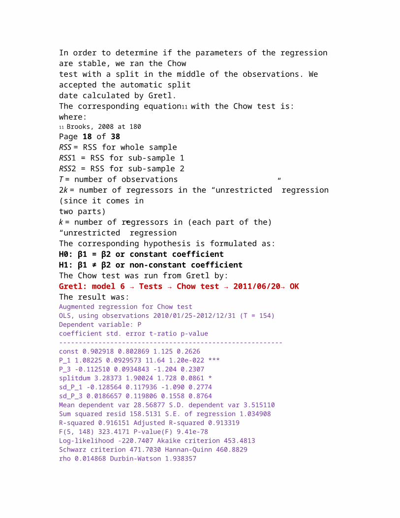
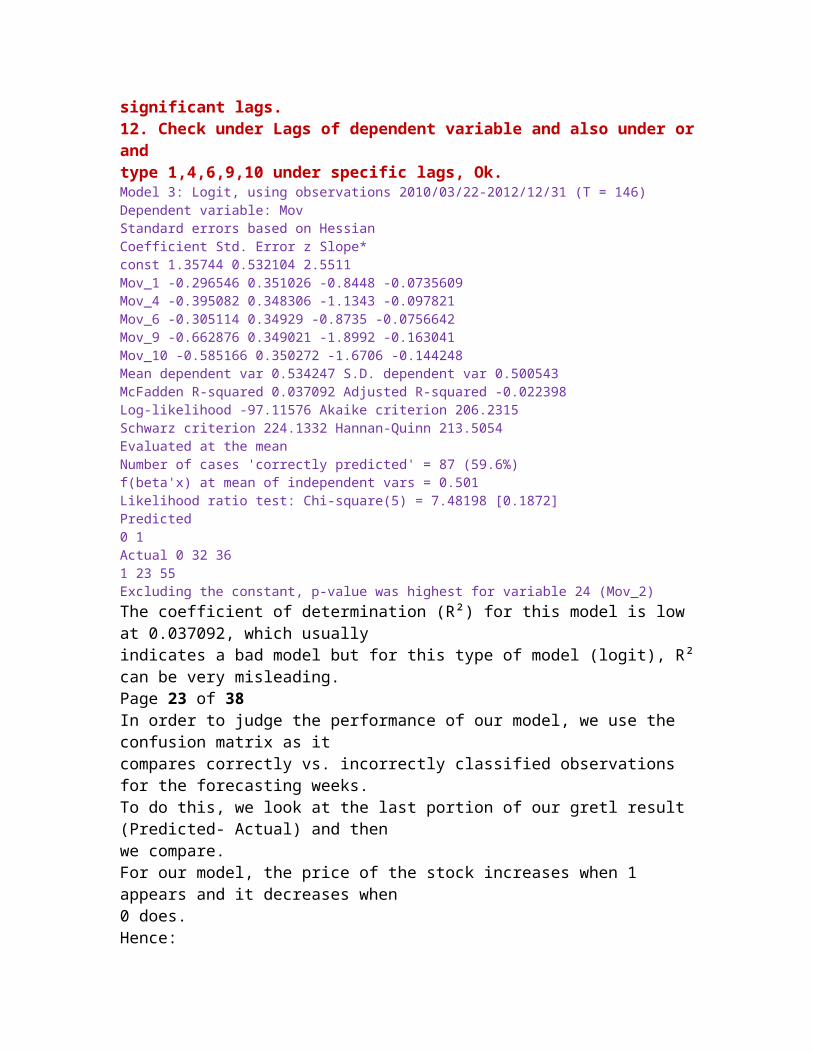