real estate and the stock market: a meta-regression analysis

REAL ESTATE AND THE STOCK MARKET:

A META-REGRESSION ANALYSIS

Authors: Deirdre Reilly, Brian Lucey and Constantin Gurdgiev

Institution: Trinity College Dublin

ABSTRACT

The real estate finance literature provides diverse and contradictory findings regarding the

distribution of real estate returns and the linkage between these returns and stock market returns.

Despite the importance of this relationship to the economy in general relatively little is known of

what causes such differences. In this paper, through applying the technique of meta-regression

analysis to the empirical studies in the area a significant step is made towards objectively

integrating and synthesising the results and identifying systematic variations in the results of

studies.

1

1. INTRODUCTION

The distributional properties of the returns of common stocks have been the subject of numerous

empirical studies. Analysis of kurtosis in the equity market dates back as far as Mandelbrot (1963)

and Fama (1965). For real estate assets, there exists a substantial body of research investigating the

first two moments of returns (mean and variance), however analyses of the third and fourth

moments (skewness and kurtosis) is very limited. The overwhelming majority of studies that do

investigate these four properties find real estate returns to be non-normally distributed. There is

little, if any, concrete analysis of what are the factors affecting the degree of non-normality, or in

the case where returns are found to be normally distributed (Lizeri and Ward,1997; Seiler et al.,

1999; Brown and Matysiak, 2000), what are the features of such studies.

Despite the importance of real estate assets to the general economy, surprisingly little is known of

how such assets interact with other macroeconomic variables. There is much disagreement in

literature regarding the nature of the relationship between real estate prices and the stock market.

There is mixed evidence as to whether such a relationship actually exists, and where one is found

on the size and direction of the relationship. The lack of an extended period of analysis and the

omission of structural change periods in existing literature has led to confusion regarding the

nature of any relationship.

The purpose of this paper is to overcome many of these limitations by employing meta-regression

analysis to integrate and summarize in a statistically meaningful way disparate extant research

results. By combining studies, a longer period of analysis is achieved that will incorporate the

various cycles and shifts over time for which data was recorded and studied, leading to more

accurate and meaningful results. Seiler et al. (1999) argues that studies of REIT performance

should use as long a time period as possible as real estate has probably experienced the greatest

number of booms and busts of any investment asset and as such this has lead to conflicting results

in studies. Meta-regression analysis can improve the assessment of this important relationship by

merging all of the existing estimates and investigating the sensitivity of the overall estimate to

variations in the underlying studies. Furthermore, meta-regression analysis provides a method of

quantitatively reviewing the empirical literature in a systematic and objective framework.

In this paper, three related but independent issues will be analyzed by meta-regression analysis:

(1) The degree of normality in real estate returns distributions, (2) To what extent has the literature

confirmed that real estate returns and stock market returns are correlated, and (3) What is the

effect of stock market returns on real estate returns?

2. EMPIRICAL RESEARCH ON THE DISTRIBUTION OF REAL ESTATE RETURNS

AND THE RELATIONSHIP BETWEEN REAL ESTATE RETURNS AND STOCK

MARKET RETURNS

The assumption of normality of the return distribution for direct (private) real estate returns and

returns of real estate securities has been rejected in many studies (Myer and Webb, 1994, Byrne

and Lee, 1997; Liow and Chan, 2005, Liu et al., 1992). There is considerable disagreement as to

the direction of skewness of returns. Lizieri and Satchell (1997) and Brown and Matysiak (2000)

have found returns to be positively skewed, Myer and Webb (1991), Knight et al. (2005) and

Okunev (2000) found that they were negatively skewed, while within the one study Maurer et al.

2

(2004) and Pagliari and Webb (1995) found some return series to be positively skewed and others

to be negatively skewed. The vast majority of studies concluded that real estate returns displayed

excess kurtosis, (Myer and Webb, 1994; Byrne and Lee, 1997; Liow and Chan, 2005; Young et al.,

2006).

Hutson and Stevenson (2008) examined the asymmetry in daily REIT returns and found skewness

to be inversely related to the index’s relative performance. In contrast, Bond and Patel (2003)

found little evidence of time variation in the skewness parameters of REIT returns. Brounen et al.

(2008) find property shares to be non-normally distributed, with kurtosis decreasing in all markets

over time. Furthermore, kurtosis is found to be greatest among property stocks which have a high

volume traded, are geographically specialised and have a small market capitalisation.

There is much disagreement in literature regarding the nature of the relationship between real

estate prices and the stock market. As a starting point to many studies, the mostly commonly

reported variable is the correlation between real estate returns and stock market returns. There is

huge disparity in the size and direction of this variable – ranging from a negative correlation of

0.32 (Miles and McCue, 1984) to a positive correlation of 0.89 (Gyourko and Keim, 1992). Very

high correlations are mostly reported for the US (Gyourko and Keim, 1992; Brown & Matysiak,

2000; Clayton and MacKinnon, 2001; Ghosh et al., 1996; Mei and Lee, 1994).

Standing out from these is Brown & Matysiak (2000) which reported a correlation of 0.86 for UK

commercial real estate returns. Apart from being based in the US, the majority of studies which

found high correlations looked at REIT returns or property share returns. Nevertheless even some

of those analyzing REIT returns in the US found negative to small positive correlations - Miles

and McCue, 1984 (-0.32), Goldstein and Nelling, 1999 (-0.04) and Ghosh et al., 1996 (0.07).

Differences in the time period of analysis may have a role to play in these results as both Miles

and McCue (1984) and Goldstein and Nelling (1999) began their analysis in the early 1970s, much

earlier than the vast majority of these studies. Small capitalization stock returns appear to have a

higher correlation with real estate returns than large capitalization stocks. Mei and Lee (1994) are

the only study looking at small capitalization stocks that reported a negative correlation (-0.04).

Below a positive correlation of 0.25 there are very few studies that look at small capitalization

stocks.

Similarly, significant disparity exists in the findings of studies which estimate the effect of real

estate returns on stock market returns. Tse (2001), Qikarinen (2006), Okunev et al. (2000) and

Aperergis and McGuire (2007) find a significant inter-relationship between the two markets, while

Quan and Titman (1997), Yunus (2008) and Beltratti and Morana (2010) find a relationship in

some countries but not in others. However, there is still considerable disagreement between the

studies relating to the size, direction and nature of the relationship.

Liow and Yang (2005) find the housing and stock markets to be cointegrated, Chen et al. (2009)

finds cointegration in some time periods, while Qkunev and Wilson (1995) believe the markets are

fractionally cointegrated. In some studies, the real estate market is found to have a strong granger

causality effect on the stock market, with Okunev et al. (2000) reporting a stock market coefficient

of 1.67. However, using a similar method the findings of Yunus (2008) suggest that the real estate

market does not have any granger causality effect on the stock market.

3

While most of the literature is US based, some authors have examined the relationship in an

international context, either by analyzing other countries individually or through panel data

analysis. By examining a larger set of countries, panel data analysis attempts to increase the

number of observations and hence the reliability of the results. Mixed findings stem from such

methods of analysis. Quan and Titman (1997) find a stock coefficient of 0.53 when doing a panel

data analysis of 7 Asian countries between 1979 and 1984. However, in a later paper by the same

authors (1999) a panel data analysis of 6 European economies between 1983 and 1996 reveals a

stock coefficient of -0.5. Cross sectional studies also produce mixed results. Quan and Titman

(1997) utilize cross section data to allow for a longer holding period while still having sufficient

data to examine the relationship between real estate and stock returns. Over a 7 year holding

period, the stock coefficient found to be 0.53. However, in their later study (1999) of 14 different

countries, cross sectional results for the same length of holding period ranged from 0.2 to 0.47

depending on the period of the study and whether rental rates or capital values were analyzed.

As with the literature of the correlation between real estate returns and stock market returns,

analysis of the effect of the real estate market on the stock market generally found the largest

positive effects in the US (Okunev et al., 2000; Liang et al., 1995; Okunev and Wilson, 1997;

Clayton and MacKinnon, 2001). However, this is not always the case as an analysis of the US

market by Glascock et al. (2000) revealed that the real estate market had a negative effect on the

stock market of -2.06 between 1992 and 1996.

Studies examining the returns to REITs or property shares, as opposed to commercial property or

housing assets, generally found a higher positive effect of these real estate assets on the stock

market. Okunev et al. (2000) found a stock coefficient of 1.67 in a granger causality test of the

effect of Equity REITs on the S&P500 between 1989 and 1998. Using a two index market model,

Liang et al. (2005) revealed a stock coefficient of 1.08 in the relationship between Hybird REITs

and NYSE/ASE market return index between 1973 and early 1989. However, on the other end of

the scale, Glascock et al. (2000) based his strongly negative stock coefficient value on the

relationship between Mortgage REITs and the S&P500.

3. META REGRESSION ANALYSIS: APPROACH

Stated simply, “meta-regression analysis is the regression analysis of regression analyses”, Stanley

and Jarrell (1989:299). It provides a means of removing the subjectivity in literature surveys and

objectifying the review process. Unlike a traditional literature review where the review chooses

which studies to include, what weight to give to each to the results of each study and how to

interpret the finding, with meta-regression analysis all relevant studies are included, the results are

weighted objectively based on their expected accuracy or reliability and the process of analysis

integrates and summarises the results to provide estimates of empirical magnitudes and to

determine what factors cause variations in the results.

Meta-regression analysis is becoming increasingly popular in the social sciences, including

economics and finance, as a means of examining and combining different research results on a

given issue. It is particularly useful where alternative specification and assumptions lead to

conflicting results. The advantages of using the technique of meta-regression analysis is best

explained in the seminal work of Stanley and Jarrell (1989:300): “Meta-regression analysis not

4

only recognises the specification problem but also attempts to estimate its effects by modeling

variations in selected econometric specifications. Meta-regression analysis provides us with the

means to analyze, estimate, and discount, when appropriate, the influence of alternative model

specification and specification searches. In this way, we can more accurately estimate the

empirical magnitudes of the underlying econometric phenomena and enhance our understanding of

why they vary across the published literature.”

Meta-regression analysis developed from a popular technique, particularly in medical research,

called meta-analysis. From each study, meta-analysis calculates the effect size, w = (ue – uc)/σc,

where ue is the mean of one group (generally the experimental group), uc is the mean of the control

group and σc is the standard deviation of the control group. The effect size w is used to compare

the parameter estimates from various studies. This standardised statistic provides a means of

consistently interpreting in a numerical fashion the results of highly individualised studies across

all variables and measures involved, (Lispey and Wilson, 2001). However, the applicability of this

technique to finance and economics is limited because it is rare to encounter studies with

experimental and control groups. Unlike effect size, in the context of a regression, there are units

of measurement attached to a regression coefficient. Analogous to the effect size would be the

reported t-statistic associated with the regression coefficient. A t-statistic does not have

dimensionality and therefore is a standardised measure of the critical parameter of interest,

(Stanley and Jarrell, 1989).

A further limitation of meta-analysis is that it fails to address the question of what are the key

differences that cause variation among the studies results. Meta-regression analysis attempts to

overcome these limitations by explaining the assumptions and specifications that systematically

affect the results of studies.

A typical meta-regression model takes the form:

bi = β + ∑Kk=1αkXik + ei i = 1,2,...L.

where bi is the is the reported estimate of the statistic of β of the ith

study in the literature totalling

L studies, β is the “true” value of the parameter of interest, Xik is the meta-independent variable

which measures the relevant characteristics of an empirical study, αk the meta-regression

coefficient that indicates the effect of particular study characteristics and ei denotes the meta-

regression disturbance term.

Stanley (2001) outlines five steps for conducting a meta-regression analysis, as follows:

1. Include all relevant studies from a standard database

2. Choose a summary statistic and reduce the evidence to a common metric

3. Choose moderator variables

4. Conduct a meta-regression analysis

5. Subject the meta-regression analysis to specification testing

Following these five steps the three meta-regression analyses of this paper serve the purpose of

assessing:

5

Regression (1) The degree of normality in real estate returns distributions,

Regression (2) To what extent has the literature confirmed that real estate returns and stock market

returns are correlated, and

Regression (3) What is the effect of stock market returns on real estate returns?

3.1 All Relevant Studies

An extensive search for articles relating to the relationship between real estate returns and stock

market returns was conducted in the EconLit, IDEAS, SSRN and JSTOR databases. Further

studies were found from an internet search using the Irish Google search engine (www.google.ie)

and the Google Scholar search engine (www.scholar.google.com). Studies that were cited in any

of these articles were found, studies cited in the found cited articles were found, and this process

continued until no new studies were cited. Although the literature search process was designed to

be comprehensive, it cannot be guaranteed that all relevant studies were found. This may be due to

the search process or to publication selection bias, where editors tend only to publish significant

results. A number of studies that were found through the search process did not contain the

necessary information and were disregarded.

Most studies contained more than one set of relevant results. As suggested by Stanley and Jarrell

(1998) multiple observations from the same study were recorded as separate observations if they

came from different time periods or had different models. Similarly, multiple observations from

the same study, with the same time and model estimates but in different geographies, were

recorded as separate observations. Estimates from similar studies reported in different articles by

the same author using the same data were also recorded as separate observations.

The search process for relevant articles for the first meta-regression analysis resulted in 19 studies

with 182 observations, for the second meta-regression analysis there were 17 studies with 168

observations and for the third meta-regression analysis there were 9 studies with 128 observations.

Table A1, A2 and A3 in the Appendix, list the papers from which studies were drawn.

3.2 Parameter of Interest

In the meta-regression analysis accessing the normality of real estate returns, the parameter of

interest was chosen as the Jarque-Bera (JB) statistic. It is a goodness-of-fit measure of departure

from normality, based on the sample skewness and kurtosis. While the test suffers from limitations

(eg. over rejection of null hypothesis of normality in small samples), it was chosen as it was the

most widely reported test of normality of the return distribution and could be calculated from the

sample skewness and kurtosis parameters when it wasn’t directly reported. Papers which reported

findings for excess returns, log returns, differentiated returns, etc were excluded from the meta-

regression analysis.

Ideally the parameter of interest for the second meta-regression analysis would be the value of the

correlation between real estate returns and stock market returns as this variable is widely reported

in studies of the relationship between real estate and the stock market. However, this variable has

http://www.google.ie/

http://www.scholar.google.com/

6

some undesirable properties due to its inherent standardisation that yields correlations ranging

from -1 to +1 regardless of the numerical values of the underlying data to which it is applied.

Therefore, correlations are generally transformed using Fisher’s Zr-transform, defined as

ESzr = .5loge[(1+r)/(1-r)],

where r is the correlation coefficient and loge is the natural logarithm. For ease of interpretation,

the Zr-transformed correlations are translated back into standard correlation form in the results,

using the inverse of the Zr-transformation.

The parameter of interest for the third meta-regression analysis was chosen as the coefficient of

the stock market variable in the regression of stock market returns on real estate returns. While

less widely reported than the correlation, this parameter of interest is both important and

interpretable in the relationship between real estate returns and stock market returns.

3.3 Moderator (Meta-Independent Variables)

This step in the meta-regression analysis process requires the choice of moderator, predictor or

meta-independent variables. Such variables can be continuous or binary variables reflecting the

presence or absence of study characteristics.

The binary variables used in the first meta-regression analysis reflect the frequency of the data, the

methodology employed, the region of the study and the property type. The frequency of the data is

analysed because it has been argued in real estate literature that for some real estate assets,

particularly commercial property, quarterly returns may be autocorrelated or that the valuations are

out-of-date as they are not conducted quarterly on each property and therefore a longer time period

should be used, (Seiler et al., 1999). However, using longer frequency data accentuates the

problems associated with small sample sizes, particularly for real estate, where in most case the

time period of the data is relatively short. Also, Liow and Chan (2005) forward normality is less

likely to hold for more frequently observed real estate return data. A binary variable to reflect the

methodology used in the study was inserted to capture any differences in the results due to using

non-conventional methodology. Most papers simply calculated the JB statistic on the returns, but

in some cases an autoregressive model was used to remove autocorrelation in the series. The

region of the studies data was examined to investigate if this affected the degree of normality in

the returns series. The property type under consideration has been suggested to impact on the

distribution of returns. Bond and Patal (2003) argue that securitized real estate are more accurately

reflects real estate returns than commercial real estate because it avoids the need to de-smooth the

appraisal based indices used in the latter and hence the uncertainty surrounding the method chosen

to correct the data. Securitized real estate also provides a longer period of data, which can capture

more of the cycles in the data.

The second and third meta-regression analysis use binary variables to reflect the frequency of the

data, the region of the study, the property type and the stock type. The frequency of the data is

analysed as it has been proposed in literature that relatively long measurement intervals are

required to observe a relationship between the real estate market and the stock market, (Quan and

Titman, 1999). The region of study is examined because it has been debated in literature whether

this is a significant factor determining the relationship between real estate returns and stock market

7

returns, (Quan and Titman, 1996; Yunus, 2008). Contrasting results in the empirical literature

involving various property and stock types drives the inclusion of these as independent variables,

(Miles and Cue, 1984; Gyourko and Keim, 1992; Eichholtz and Hartzell, 1996). Further to these

variables, in the second meta-regression analysis binary variables are also included to reflect the

methodology of the study as it is commonly recognised that differences in this factor can have a

major impact on a study’s findings.

The continuous variables used for all three meta-regression analysis are, the year of the data, the

year of publication of the article, the number of observations, the number of authors of the article

and finally, for the third meta-regression analysis, also included is the p-value for the coefficient

on the stock market variable. The year of the data is included as independent variables to capture

changes over time in the observed relationship due to different periods of data used in the analysis,

while year of publication is inserted to highlight systematic changes in the results of studies

conducted during different time periods. The number of authors is analysed to investigate if this

could influence the observed relationship, perhaps multi-author papers reporting more

conservative results. The number of observations is a reliability measure which is used to weight

the results in the first and second regression and as a moderator variable in the third regression.

Similarly, the reported p-value is a reliability and accuracy measure that is used to weight the

results of the third regression.

Refer to the Appendix for comprehensive definitions of the meta-independent variables, and for

tables containing the parameters of interest and their respective meta-independent variable study

characteristics.

Table 1 shows the correlations among the variables in the first meta-regression. As can be

expected the year of publication and the mid-point of the time period analysed are highly

correlated. The high negative correlation between the region and the year of the data is due to the

earlier data availability and research for the US compared to other regions. High correlation

among the moderator variables generally reduces the significance of the individual variables

coefficients in the meta-regression analysis, although together they may be jointly very significant

the effect of one cannot be distinguished from the effect of the other. For this reason, it was

decided to omit the year of publication from the regression.

Table 1: Meta-Regression 1 - Correlation Matrix

Variables JB TEST No.

Authors

Frequency Methodology No.

Observations

Property

Type

Region Year of

data

Year of

publication

JB TEST 1.00 0.03 0.06 0.06 0.63 0.32 -0.01 0.36 0.34

No. Authors 0.03 1.00 -0.29 0.09 -0.03 0.28 -0.02 0.07 0.16

Frequency 0.06 -0.29 1.00 -0.12 0.15 0.13 0.06 -0.02 -0.14

Methodology 0.06 0.09 -0.12 1.00 0.05 0.17 -0.19 0.17 0.16

No. Observations 0.63 -0.03 0.15 0.05 1.00 0.32 0.17 0.43 0.31

Property Type 0.32 0.28 0.13 0.17 0.32 1.00 -0.03 0.25 0.18

Region -0.01 -0.02 0.06 -0.19 0.17 -0.03 1.00 -0.55 -0.55

Year of data 0.36 0.07 -0.02 0.17 0.43 0.25 -0.55 1.00 0.93

Year of

publication 0.34 0.16 -0.14 0.16 0.31 0.18 -0.55 0.93 1.00

8

Table 2 shows the correlations among the variables in the meta-regression 2. Similar to the

previous regression, the year of publication and the mid-point of the time period analysed are

highly correlated. The property type and frequency of the data are highly correlated. REITs,

property shares and property mutual funds tended to have a higher frequency than would other

property assets, such as commercial property and housing assets. Similarly, there is a quite high

correlation between property type and region due to the relatively high quantity of REITs located

in the US. To avoid multi-colinearity, it was decided to omit the year of publication and the

frequency from the meta-regression 2.

Table 2: Meta-regression 2 - Correlation matrix

Variables Zr-

transforme

d

correlation

Year of

publicatio

n

Year of

data

No.

authors

No.

observatio

ns

Region Frequenc

y

Property

type

Stock

type

Zr-transformed

correlation

1.00 0.08 -0.08 -0.12 0.19 0.27 0.14 0.42 -0.37

Year of

publication

0.08 1.00 0.62 -0.35 0.14 -0.14 -0.26 -0.26 0.20

Year of data -0.08 0.62 1.00 0.17 -0.14 -0.31 -0.06 -0.02 0.04

No. authors -0.12 -0.35 0.17 1.00 -0.22 0.13 0.34 0.37 -0.32

No.

observations

0.19 0.14 -0.14 -0.22 1.00 0.31 0.34 0.37 -0.12

Region 0.27 -0.14 -0.31 0.13 0.31 1.00 0.35 0.42 -0.43

Frequency 0.14 -0.26 -0.06 0.34 0.34 0.35 1.00 0.60 -0.33

Property type 0.42 -0.26 -0.02 0.37 0.37 0.42 0.60 1.00 -0.43

Stock type -0.37 0.20 0.04 -0.32 -0.12 -0.43 -0.33 -0.43 1.00

Table 3 shows the correlations among the variables in the meta-regression 3. The results are

similar to those of the meta-regression 2, however more pronounced. The year of publication and

the mid-point of the time period have a correlation coefficient of 0.68. In this case the property

type and the frequency are perfectly positively correlated, and both have correlation of 0.93 with

the region. To avoid multi-colinearity in the meta-regression 2 it was decided to omit frequency,

region and year of publication.

9

Table 3: Meta-regression 3 - Correlation matrix

Variables Stock coeffi-

cient

P -value

Year of

public-

ation

Year of

data

No. autho-

rs

No. Obser-

vations

Regi-on

Freq-uency

Proper-ty type

Stock type

Cointe-gration

Cross section

/panel

Granger Causali-

ty

Stock coefficient

1.00 -0.59 -0.29 -0.46 0.08 0.20 0.16 0.16 0.16 -0.12 -0.33 -0.09 0.19

P -value -0.59 1.00 0.05 0.21 -0.01 -0.36 -0.12 -0.20 -0.20 0.16 0.13 -0.22 -0.01

Year of publication

-0.29 0.05 1.00 0.68 -0.56 0.16 -0.24 -0.08 -0.08 -0.04 0.01 0.30 0.60

Year of data -0.46 0.21 0.68 1.00 -0.56 -0.17 -0.43 -0.35 -0.35 0.00 0.05 0.22 0.21

No. Authors 0.08 -0.01 -0.56 -0.56 1.00 0.03 0.65 0.57 0.57 0.09 0.11 -0.33 -0.09

No. Observations

0.20 -0.36 0.16 -0.17 0.03 1.00 0.23 0.29 0.29 -0.11 0.20 0.28 0.27

Region 0.16 -0.12 -0.24 -0.43 0.65 0.23 1.00 0.93 0.93 -0.31 0.45 -0.58 0.16

Frequency 0.16 -0.20 -0.08 -0.35 0.57 0.29 0.93 1.00 1.00 -0.31 0.45 -0.58 0.31

Property type 0.16 -0.20 -0.08 -0.35 0.57 0.29 0.93 1.00 1.00 -0.31 0.45 -0.58 0.31

Stock type -0.12 0.16 -0.04 0.00 0.09 -0.11 -0.31 -0.31 -0.31 1.00 -0.44 0.18 0.05

Cointegration -0.33 0.13 0.01 0.05 0.11 0.20 0.45 0.45 0.45 -0.44 1.00 -0.26 -0.07

Cross

section/panel

-0.09 -0.22 0.30 0.22 -0.33 0.28 -0.58 -0.58 -0.58 0.18 -0.26 1.00 -0.18

Granger

Causality

0.19 -0.01 0.60 0.21 -0.09 0.27 0.16 0.31 0.31 0.05 -0.07 -0.18 1.00

3.4 Estimation of the Meta-Regression Model

The meta-regressions are estimated using the standard meta-regression model as discussed earlier,

which takes the form:

bi = β + ∑Kk=1αkXik + ei i = 1,2,...L.

In the meta-regression 1 and 2, the constant term, β, represents the average Zr-transformed

correlation and the average stock coefficient, respectively, calculated when all the moderator

variables are zero. The Xik variables are the moderator (or meta-independent) variables that

measure characteristics of the study, such as the year of the data, the property or stock type, the

methodology used.

3.5 Specification Tests

This step involves checking that the assumptions underlying the estimation of the least squares

model used in this study are satisfied.

Considering the correlation matrix of independent variables from the three models, it is clear that

the models’ regressors are linearly independent.

For the first meta-regression, the level of the JB statistic was initially used as the dependent

variable. However, due to poor diagnostic properties of this model (eg. non-normalitiy,

instability), the log of the JB statistic was used instead. The normality of the residuals for this

10

model is indicated by the statistically insignificant JB statistic (0.09) and the histogram of

residuals, see figure A1 in the Appendix. For meta-regression model 2, the normality of the

residuals is assured from both a visual inspection of the histogram of residuals, see Figure A2 in

the Appendix, and the Jarque-Bera test which is not statistically significant, thereby failing to

rejecting the null hypothesis of normality. For the meta-regression model 3, this assumption is

harder to meet as the Jarque-Bera test is statistically significant. However, the histogram of

residuals suggests that they are distributed not unlike a normal distribution; see Figure A3 in the

Appendix.

In all three models, White heteroskedasticity consistent covariance estimates are used to provide

consistent parameter estimates in the presence of heteroskedasticity of an unknown form.

Ramsey’s RESET test which provide a general test for misspecification of the errors, for example,

omitted variables, incorrect functional form and correlation between the independent variables and

the disturbance term, failed to detect specification error in either model.1

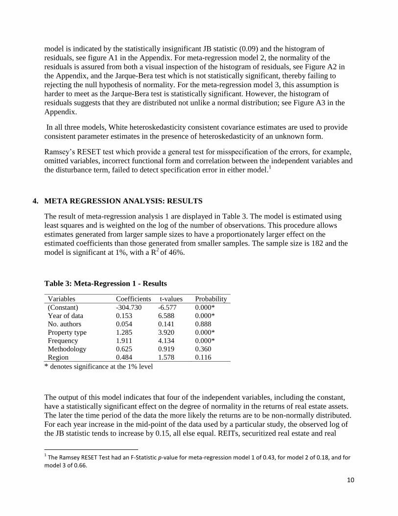
4. META REGRESSION ANALYSIS: RESULTS

The result of meta-regression analysis 1 are displayed in Table 3. The model is estimated using

least squares and is weighted on the log of the number of observations. This procedure allows

estimates generated from larger sample sizes to have a proportionately larger effect on the

estimated coefficients than those generated from smaller samples. The sample size is 182 and the

model is significant at 1%, with a R2

of 46%.

Table 3: Meta-Regression 1 - Results

Variables Coefficients t-values Probability

(Constant) -304.730 -6.577 0.000*

Year of data 0.153 6.588 0.000*

No. authors 0.054 0.141 0.888

Property type 1.285 3.920 0.000*

Frequency 1.911 4.134 0.000*

Methodology 0.625 0.919 0.360

Region 0.484 1.578 0.116

* denotes significance at the 1% level

The output of this model indicates that four of the independent variables, including the constant,

have a statistically significant effect on the degree of normality in the returns of real estate assets.

The later the time period of the data the more likely the returns are to be non-normally distributed.

For each year increase in the mid-point of the data used by a particular study, the observed log of

the JB statistic tends to increase by 0.15, all else equal. REITs, securitized real estate and real

1 The Ramsey RESET Test had an F-Statistic p-value for meta-regression model 1 of 0.43, for model 2 of 0.18, and for

model 3 of 0.66.

11

estate mutual funds are more likely to have a greater degree of non-normality in their returns than

commercial property or housing. On average, with all else equal, the log of the JB statistic is

higher by 1.28 when considering the former rather than the later. Related to this is the observation

that the returns are more non-normal when using higher frequency data. Returns with a frequency

of quarterly or shorter, tended to have a log of JB statistic that is higher by 1.91 than if considering

annual or semi-annual data, all else equal. The region is does not appear to have a significant

effect on the normality of the returns. As the region variable is quite highly correlated with the

time period and the methodology, these were excluded variables were excluded from the model to

see whether the region would then have a significant impact on the JB statistic. The output of this

model still indicated that the region of the study did not affect the degree of normality in the real

estate returns. The methodology used in the studies and the number of authors also did not appear

to impact on the observed normality of the returns.

Table 4 displays the results from the estimation of the meta-regression analysis model 2. Similar to

model 1, this model is estimated using least squares and is weighted on the log of the number of

observations. The sample size is 168 and the dependent variable is Zr-transformed correlation. The

Zr-transformed correlations are transformed back to standard correlational form for ease of

interpretation in the results.2 The model is significant at 1% and has a R

2 of 31%.


Variables Coefficient

s

t-values Probability

(Constant) 3.341 0.731 0.466

Year of data -0.002 -0.652 0.515

No. authors -0.071 -3.781 0.000*

Property type 0.136 4.784 0.000*

Stock type -0.132 -3.705 0.000*

Region -0.016 -0.487 0.627

* denotes significance at the 1% level

Three of the meta-independent variables are highly significant – number of authors, property type

and stock type. The greater the number of authors the lower is the reported correlation. As the

number of authors increases by 1, the reported correlation decreases by 0.07, all else equal. While

this is a difficult result to explain, it may indicate that multi-author studies are conservative in their

estimations. The property type variable behaves as theoretically expected – REITs, property shares

and property mutual funds are more highly correlated with the stock market than other types of

property assets, such as commercial property and housing. This model suggests that with all else

remaining constant, REITs, property stocks and property mutual funds will have a correlation with

the stock market that is 0.14 higher than that of other assets. Again in keeping with theory, real

estate assets display a higher correlation with small capitalisation stocks than large capitalisation

stocks. For large capitalisation stocks, the correlation with real estate assets is lower by 0.13.

2 This is performed using the formula r = (e

2ESzr – 1)/ (e

2ESzr + 1). However, for a correlation matrix sufficiently distant

from the limit values of 1 and -1, the Fisher’s transformation is approximately equal to the original results.

12

Although the region is not a significant variable in this model, this may be due to its correlation

with the property type, as discussed earlier. The year of the data is insignificant, suggesting that

the correlation of real estate returns with stock market returns has not changed systematically over

time. This indicates that despite the considerable stock market and property market booms and

busts over the nearly 40 year period of the data, the average correlation between the two markets

has remained constant.

Table 5 displays the results from the estimation of the meta-regression analysis model 3. The

dependent variable is the coefficient on the stock market returns and the model is weighted by the

inverse of the p-value for coefficient. The model is estimated by least squares and has 128

observations. The model is significant at 1% and has a relatively high R2 of 66%.


Variables Coefficients t-values Probability

(Constant) 43.836 4.131 0.000*

Year of data -0.022 -4.174 0.000*

No. authors -0.075 -0.864 0.389

No. observations -0.001 -2.164 0.032**

Property type 0.682 3.060 0.003*

Stock type 0.086 2.365 0.020**

Cointegration 0.100 1.289 0.200

Cross section/panel 0.477 2.155 0.033**

Granger causality -0.118 -0.502 0.616

*denotes significance at the 1% level

**denotes significance at the 5% level

The property type and stock type are still highly significant in this model, with a significance level

of 1% and just over 1% respectively. The property type variable is economically very significant

as it indicates that the stock market coefficient is higher by 0.69 when considering the relationship

with REITs, property stocks or mutual funds rather than other real estate assets. The stock market

coefficient is higher by 0.086 when analysing the relationship between large capitalisation stocks

and real estate assets, than when studying small capitalisation stocks and real estate assets. While

it is generally believed that real estate assets are closer to small capitalisation stocks than large

capitalisation stocks, it appears that real estate has a greater effect on large capitalisation stocks

than small capitalisation stocks. However, the economic significance of this variable is

considerably smaller than that of the property type.

The only methodology based independent variables which was significant was the cross

section/panel variable, which suggests that stock market coefficient in the relationship with real

estate assets is higher by 0.477 when using cross section or panel data analysis. This implies that

the relationship between the stock market and real estate assets is stronger when considering a

group of countries, rather than one country in isolation. This is intuitively appealing on two levels;

firstly, the distortions and peculiarities of individual the markets in countries may weaken the

observed relationship, however by studying a larger number of markets these effects become less

13

pronounced and the overall relationship becomes clearer, secondly, by using panel data the

number of observations in the study can be increased, which should make any existent relationship

more evident.

Unlike the meta-regression model 2, the year of the data is statistically very significant in this

model. The variable indicates that the effect of the stock market on real estate asset returns is

decreasing over time. In particular, as the mid-point of the data range of a study increases by one

year the stock market coefficient decreases by 0.022. While this is not a large value considered on

its own, cumulatively over time this would indicate a large weakening of the effect of real estate

assets on stocks. Again, unlike the meta-regression model 2, the number of authors of a study did

not have a significant affect on the results.

Included as an explanatory variable in this model, the number of observations in each study was

statistically significant at 5%. This variable indicates that the larger the number of observations the

lower the observed effect of the stock market on real estate assets. As the number of observations

in a study increases by one, the stock coefficient decreases by 0.001. Considering as a study of this

kind can vary largely on the number of observations used, this variables suggests that it can have a

large effect on the studies findings. Furthermore, if we assume that a studies’ reliability increases

with the number of observations, this indicates that the more reliable studies find the stock market

has a smaller effect on real estate assets.

5. CONCLUSIONS

Over the past 40 years, researchers have been analysing the distribution of real estate returns and

over the past 30 years several studies have empirically analysed the relationship between real

estate returns and stock market returns. However, from studying bibliographic databases, this

paper appears to be the first attempt to quantitative synthesis these studies by means of meta-

regression analysis. Through this process limitations of the original studies, for example, shortage

of data and model misspecification can be controlled for. Overcoming the restrictions, subjectivity,

and dissonance of traditional literature reviews, meta-regression analysis allows the results of all

relevant studies be objectively integrated and the sensitivity of these results to various factors

analysed. In an economically and financially important area of study, where there is little research

on the causes of non-normality in real estate returns and little consensus on the nature of the

relationship between real estate and stock market returns, not least the factors influencing this

relationship, this paper provides a significant step forward in the research.

The first meta-regression analysis model explained 46% of the variation in the JB statistic. It was

found that real estate returns have a higher degree of non-normality the later the time period of the

study, indicating that returns are getting less normal over time. Higher frequency data also caused

the returns to display less normality. Related to this was the finding that REITs, securitized real

estate and real estate mutual funds had a lower degree of normality than other real estate assets,

such as commercial real estate or housing.

In the second meta-regression analysis, 31% of the variation in the correlation between models

was explained by variation in the independent regressors. The property type and stock type

analysed significantly affected the findings of the study. As would be expected, REITs, property

shares and property mutual funds were more closely correlated with the stock market than other

14

types of property, such as commercial property and housing. Similarly, real estate returns were

more highly correlated with small capitalisation stocks than large capitalisation stocks. The greater

the numbers of authors to a paper, the more likely the results are to report a lower correlation. This

may be a spurious result, or perhaps indicate that multi-author papers are more conservative in

their results. Interestingly, the time period and region studied did not significantly influence the

results.

The third meta-regression model managed to explain 66% of the variance in the stock coefficient

by the variance in the moderator variables. Once again, both the property type and stock type were

statistically significant. With a higher statistical and economic significance, and in line with

theory, the property type coefficient indicated that REITs, property shares and property mutual

funds had a greater effect on the stock market than other real estate assets. The stock type

coefficient suggested that real estate assets had a greater effect on large capitalisation stocks than

small capitalisation stocks. Importantly for investors who may be trying to diversify assets, the

findings indicate that the effect of the stock market on real estate has systematically reduced over

time. The number of observation is found to reduce the observed effect, perhaps flagging that the

more reliable results find a smaller relationship. Where the study uses cross section or panel data,

the reported effect of the stock market on real estate is greater. This suggests that on an aggregated

level the effect of the stock market on real estate is greater than when individual markets are

considered in isolation. Other methodologies used by studies did not appear to significantly affect

the results. Unlike the previous analysis, the second meta-regression analysis did not find the

number of authors to have a significant affect on the results.

Considering the results of the three meta-regression analysis, it appears that the property type has

an important effect on the properties displayed by the real estate asset. Related to this is the

frequency and region, both of which can be quite highly correlated with the property type.

However, these do not display the same level of influence on the results. The stock type is also

very significant in the nature of the relationship observed between the stock market and real estate

assets. The time period of the data was an important factor in two of the three meta-regressions.

The impact of the methodology used by researchers on the results has yet to be confirmed as it was

not important in the first meta-regression, it did not apply to the second model and only one of the

three methodologies tested for in the third meta-regression was significant. The number of authors

to a paper does not play a notable part in two of the three meta-regressions and therefore it is

questionable whether differences in the number of authors influence the results of research.

Further analysis of the empirical literature in the area of real estate finance is required to provide

some consensus, meaningfulness and significance to the disparate results of various studies. Such

analysis requires a sufficient number of studies using the same metric of analysis for the dependent

variable and is therefore somewhat restricted in the specific questions that may be analysed using

this methodological tool.

15

APPENDIX

Table A1: Meta-Regression Analysis 1: List of Papers

Author Year

Myer and Webb 1994

Byrne and Lee 1997

Liow and Chan 2005

Hutson and Stevenson 2008

Brounen et al. 2008

Myer and Webb 1993

Lizieri 2007

Pagliari and Webb 1995

Maurer et al. 2004

Myer and Webb 1991

Coleman and Mansour 2005

Chiang et al. 2008

Cotter and Stevenson 2008

Lizieri and Satchell 1997

Cotter and Stevenson 2006

Brown 1991

Brown and Matysiak 2000

Miles and McCue 1984

Okunev et al. 2000

16

Table A2: Meta-Regression Analysis 2: List of Papers

Author Year

Gyourko and Keim 1992

Brown 1991

Brown & Matysiak 2000

Clayton and MacKinnon 2001

Eichholtz and Hartzell 1996

Ghosh et al. 1996

Goldstein and Nelling 1999

Hartzell et al. 1986

Laopodis 1999

Lizieri and Satchell 1997

Maurer et al. 2004

Mei and Lee 1994

Miles and McCue 1984

Oikarinen 2006

Quan and Titman 1999

Sing and Ling 2003

Wurtzebach et al. 1995

Table A3: Meta-regression analysis 3: List of papers

Author Year

Clayton and MacKinnon 2001

Glascock et al. 2000

Li and Wang 1995

Liang et al. 1995

Okunev and Wilson 1997

Okunev et al. 2000



Yunus 2008

17

Meta-Regression Analysis 1: List of Meta-Independent Variables and Definitions

Year of publication

Year of the data – The mid-point of the data range of the study

Number of authors

Number of observations

Region – 1 if US; 0 otherwise

Frequency – 1 if quarterly or more frequent; 0 if less frequent than quarterly

Methodology – 1 if conventional, basic model; 0 if otherwise, eg. auto-regressive model

Property type – 1 if REIT, property share or property mutual fund; 0 otherwise


Year of publication


Number of authors



Frequency – 1 if quarterly or monthly; 0 if less frequent than quarterly


Stock type – 1 if large capitalization stock; 0 otherwise


Year of publication


Number of authors



Frequency – 1 if quarterly or monthly; 0 if less frequent than quarterly


Stock type – 1 if large capitalization stock; 0 otherwise

Cointegration – 1 if cointegration analysis employed; 0 otherwise

Cross section/panel – 1 if cross section or panel data analysis employed; 0 otherwise

Granger causality – 1 if granger causality analysis employed; 0 otherwise

18

Figure A1: Meta-Regression Analysis 1 – Histogram of Standardized Residuals


0

4

8

12

16

20

24

-6 -4 -2 0 2 4

Series: Standardized Residuals

Sample 1 182

Observations 182

Mean -0.095133

Median -0.131686

Maximum 5.315204

Minimum -6.870164

Std. Dev. 1.887224

Skewness 0.174246

Kurtosis 3.707848

Jarque-Bera 4.720596

Probability 0.094392

0

2

4

6

8

10

12

14

16

-0.250 -0.125 -0.000 0.125 0.250 0.375 0.500


Sample 1 168

Observations 168

Mean 0.001091

Median 0.004840

Maximum 0.514617

Minimum -0.341459

Std. Dev. 0.144005

Skewness 0.335357

Kurtosis 3.357394



19


0

5

10

15

20

25

30

35

-0.4 -0.2 -0.0 0.2 0.4 0.6 0.8


Sample 1 128

Observations 128

Mean 0.003323

Median -0.009581

Maximum 0.791810

Minimum -0.475517

Std. Dev. 0.189758

Skewness 1.418875

Kurtosis 8.595312



20

BIBLIOGRAPHY

APERGIS, N. & LAMBRINIDIS, L. 2007. More Evidence on the Relationship between the Stock and

Real Estate Market. Working Paper Series [Online]. [Accessed 14 September 2010].

BELTRATTI, A. & MORANA, C. 2010. International House Prices and Macroeconomic Fluctuations.

Journal of Banking and Finance, 34, 533-545.

BOND, S. A. & PATEL, K. 2003. The Conditional Distribution of Real Estate Returns: Are Higher

Moments Time Varying? The Journal of Real Estate Finance and Economics, 26, 319-339.

BROUNEN, D., PORRAS PRADO, M. & STEVENSON, S. 2008. Kurtosis and Consequences – The

Case of International Property Shares.

BROWN, G. R. 1991. Property Investment and the Capital Markets, E & FN Spon.

BROWN, G. R. & MATYSIAK, G. A. 2000. Real Estate Investment: A Capital Market Approach,

Harlow, Financial Times Prentice Hall.

BYRNE, P. & LEE, S. 1997. Real Estate Portfolio Analysis under Conditions of Non-Normality: The

Case of NCREIF. Journal of Real Estate Portfolio Management, 3, 37-46.

CHIANG, T. C., LEAN, H. H. & WONG, W.-K. 2008. Do REITs Outperform Stocks and Fixed-Income

Assets? New Evidence from Mean-Variance and Stochastic Dominance Approaches. Working

Paper Series [Online].

CLAYTON, J. & MACKINNON, G. 2001. The Time Varying Nature of the Link between REIT, Real

Estate and Financial Asset Returns. Journal of Real Estate Portfolio Management, 7, 43-54.

COLEMAN, M. S. & MANSOUR, A. 2005. Real Estate in the Real World: Dealing with Non-Normality

and Risk in an Asset Allocation Model. Journal of Real Estate Portfolio Management, 11, 37-53.

COTTER, J. & STEVENSON, S. 2006. Multivariate Modeling of Daily REIT Volatility. Journal of Real

Estate Finance and Economics, 32, 305-325.

COTTER, J. & STEVENSON, S. 2008. Modeling Long Memory in REITs. Real Estate Economics, 36,

533-554.

EICHHOLTZ, P. M. A. & HARTZELL, D. J. 1996. Property Shares, Appraisals and the Stock Market:

An International Perspective. Journal of Real Estate Finance and Economics, 12, 163-178.

FAMA, E. F. 1965. The Behaviour of Stock Market Prices. Journal of Business, 38, 34-105.

GHOSH, C., MILES, M. & SIRMANS, C. F. 1996. Are REITs Stocks? Real Estate Finance, 13, 46-53.

21

GLASCOCK, J. L., LU, C. & SO, R. W. 2000. Further Evidence on the Integration of REIT, Bond, and

Stock Returns. Journal of Real Estate Finance and Economics, 20, 177-194.

GOLDSTEIN, M. A. & NELLING, E. F. 1999. REIT Return Behaviour in Advancing and Declining

Stock Markets. Real Estate Finance, 15, 68-77.

GYOURKO, J. & KEIM, D. B. 1992. What Does the Stock Market Tell Us About Real Estate Returns?

Journal of the American Real Estate and Urban Economics Association, 20, 457-485.

HUTSON, E. & STEVENSON, S. 2008. Asymmetry in REIT returns. Journal of Real Estate Portfolio

Management, 14, 105-123.

KNIGHT, J., LIZIERI, C. & SATCHELL, S. 2005. Diversification When it Hurts? The Joint

Distributions of Real Estate and Equity Markets. Journal of Property Research, 22, 309-323.

LAOPODIS, N. 2009. REITs, the Stock Market and Economic Activity. Journal of Property Investment

and Finance, 27, 563-578.

LI, Y. & WANG, K. 1995. The Predictability of REIT Returns and Market Segmentation. The Journal of

Real Estate Research, 10, 471-482.

LIANG, Y., MCINTOSH, W. & WEBB, J. R. 1995. Intemporal Changes in the Riskiness of REITs. The

Journal of Real Estate Research, 10, 427-443.

LING, D. C. & NARANJO, A. 1999. The Integration of Commercial Real Estate Markets and Stock

Markets. Real Estate Economics, 27, 483-515.

LIOW, K. H. & CHAN, L. C. W. J. 2005. Co-Skewness and Co-Kurtosis in Global Real Estate Securities.

Journal of Property Research, 22, 163-203.

LIOW, K. H. & YANG, H. 2005. Long-Term Co-Memories and Short-Run Adjustment: Securitized Real

Estate and Stock Markets. The Journal of Real Estate Finance and Economics, 31, 283-300.

LIPSEY, M. W. & WILSON, D. B. 2001. Practical meta-analysis, Thousand Oaks, Calif. ; London, Sage.

LIU, C., HARTZELL, D. & GRISSOM, T. 1992. The role of co-skewness in the pricing of real estate.

The Journal of Real Estate Finance and Economics, 5, 299-319.

LIZIERI, C. & SATCHELL, S. 1997a. Interactions Between Property and Equity Markets: An

Investigation of Linkages in the United Kingdom 1972–1992. The Journal of Real Estate Finance

and Economics, 15, 11-26.

LIZIERI, C. & SATCHELL, S. 1997b. Interactions Between Property and Equity Markets: An

Investigation of the Linkages in the United Kingdom 1972-1992. Journal of Real Estate Finance

and Economics, 15, 11-26.

22

LIZIERI, C., SATCHELL, S. & ZHANG, Q. 2007. The Underlying Return Generating Factors for REIT

Returns: An Application of Independent Component Analysis. Real Estate Economics, 35, 569-

598.

LIZIERI, C., WARD, C., JOHN, K. & STEPHEN, S. 2001. The distribution of commercial real estate

returns. Return Distributions in Finance. Oxford: Butterworth-Heinemann.

MANDELBROT, B. 1963. The Variation of Certain Speculative Prices. Journal of Business, 36, 394-419.

MAURER, R., REINER, F. & SEBASTIAN, S. 2004. Characteristics of German Real Estate Return

Distributions: Evidence from Germany and Comparison to the U.S. and U.K. Journal of Real

Estate Portfolio Management, 10, 59-76.

MEI, J. & LEE, A. 1994. Is There a Real Estate Factor Premium? Journal of Real Estate Finance and

Economics, 9, 113-126.

MILES, M. & MCCUE, T. 1984a. Commercial Real Estate Returns. AREUEA Journal, 12, 355-377.

MYER, F. C. N. & WEBB, J. R. 1991. Are Commerical Real Estate Returns Normally Distributed. White

Paper. Chicago: NCREIF.

MYER, F. C. N. & WEBB, J. R. 1993a. Return Properties of Equity REITs, Common Stocks, and

Commercial Real Estate: A Comparison. Journal of Real Estate Research, 8, 87-106.

MYER, F. C. N. & WEBB, J. R. 1994. Statistical properties of returns: Financial assets versus

commercial real estate. The Journal of Real Estate Finance and Economics, 8, 267-282.

OIKARINEN, E. 2006. Price Linkages Between Stock, Bond and Housing Markets - Evidence from

Finnish Data. Discussion Papers [Online]. Available:

https://econpapers.repec.org/paper/rifdpaper/1004.htm [Accessed 14th September 2010].

OKUNEV, J. & WILSON, P. 1995. Using Non-Linear Test to Examine Integration Between Real Estate

and Equity Markets. Working Paper [Online]. Available: http://ideas.repec.org/p/uts/wpaper.html.

OKUNEV, J., WILSON, P. & ZURBRUEGG, R. 2000a. The Causal Relationship Between Real Estate

and Stock Markets. The Journal of Real Estate Finance and Economics, 21, 251-261.

OKUNEV, J. & WILSON, P. J. 1997. Using Nonlinear Tests to Examine Integration Between Real Estate

and Stock Markets. Real Estate Economics, 25, 487-503.

PAGLIARI, J. L. & WEBB, J. R. 1995. A Fundamental Examination of Securitized and Unsecuritized

Real Estate. Journal of Real Estate Research, 10, 381-426.

QUAN, D. C. & TITMAN, S. 1996. Commercial Real Estate Prices and Stock Market Returns: An

International Analysis. [Accessed 14th September 2010].

23

QUAN, D. C. & TITMAN, S. 1999. Do Real Estate Prices and Stock Prices Move Together? An

International Analysis. Real Estate Economics, 27, 183-207.

RUI, C., GUANGRONG, T. & QIZHONG, D. 2009. Research on the Dynamics of Volatilities between

Stock Market and Real Estate Market. Available:

http://www.eres2009.com/papers/3CChen_Rui.phf [Accessed 14th September 2010].

SEILER, M. J., WEBB, J. R. & MYER, F. C. N. 1999. Are EREITs Real Estate? Journal of Real Estate

Portfolio Management, 5, 171-181.

SING, T. F. & LING, S. C. 2003. The Role of Singapore REITs in a Downside Risk Allocation Asset

Allocation Framework. Journal of Real Estate Portfolio Management, 9, 219-235.

STANLEY, T. D. 2001. Wheat From Chaff: Meta-Analysis as Quantitative Literature Review. Journal of

Economic Perspectives, 15, 131-150.

STANLEY, T. D. & JARRELL, S. B. 1989. Meta-Regression Analysis: A Quantitative Method of

Literature Surveys. Journal of Economic Surveys, 19, 299-308.

STANLEY, T. D. & JARRELL, S. B. 1998. Gender Wage Discrimination Bias? A Meta-Regression

Analysis. Journal of Human Resources, 33, 947-973.

TSE, R. Y. C. 2001. Impact of Property Prices on Stock Prices in Hong Kong. Review of Pacific Basin

Financcial Markets and Policies, 4, 29-43.

WILSON, P., OKUNEV, J. & TA, G. 1996. Are Real Estate and Security Markets Integrated? Some

Australian Evidence. Journal of Property Valuation and Investment, 14, 7-24.

WILSON, P. J. & OKUNEV, J. 1996. Evidence of Segmentation in Domestic and International Property

Markets. Journal of Property Finance, 7, 78-97.

WURTEZEBACH, C. H., HARTZELL, D. J. & GILIBERTO, S. M. 1995. Real Estate in the Portfolio: A

New Look. Perspectives. Summer ed.: Heitman/JMB Advisory Corporation.

YOUNG, M. S., LEE, S. L. & DEVANEY, S. P. 2006. Non-Normal Real Estate Return Distributions by

Property Type in the UK. Journal of Property Research, 23, 109 - 133.

YUNUS, N. 2008. Dynamic Interaction among Securitized Property Market, Stock Market and

Macroeconomic Fundamentals: International Evidence. University of Baltimore.

real estate and the stock market: a meta-regression analysis

Documents