Working PaperInstitut für Makroökonomie

und KonjunkturforschungMacroeconomic Policy Institute

Sebastian Gechert* | Henner Will**

Fiscal Multipliers: A Meta Regression Analysis

AbstractSince the fiscal expansion during the Great Recession 2008-2009 and the current European consolidation and austerity measures, the analysisof fiscal multiplier effects is back on the scientific agenda. The number of empirical studies is growing fast, tackling the issue with manifold model classes, identification strategies, and specifica-tions. While plurality of methods seems to be a good idea to address a complicated issue, the results are far off consensus. We apply meta regression analysis to a set of 89 studies on multiplier effects in or-der to provide a systematic overview of the different approaches, to derive stylized facts and to separate structural from method-specific effects. We classify studies with respect to type of fiscal impulse, model class, multiplier calculation method and further control variab-les. Moreover, we analyse subsamples of the model classes in order to evaluate the effects of model-class-specific properties, currently discussed in the literature, such as the influence of central bank reaction functions and liquidity constrained households. As a major result, we find that the reported size of the fiscal multiplier crucially depends on the setting and method chosen. Thus, economic policy consulting based on a certain multiplier study should lay open by how much specification affects the results. Our meta analysis may provide guidance concerning influential factors.

Keywords: multiplier effects; fiscal policy; meta analysis.

JEL ref.: E27, E62, H30.

____________________

* Chemnitz University of Technology. Corresponding author, gechert@wirtschaft.tu-chemnitz.de** Macroeconomic Policy Institute. My good friend and coauthor Henner Will passed away in a tragic road accident on November 18, 2011 at the age of 28.

97Juli 2012

Fiscal Multipliers: A Meta Regression Analysis∗

Sebastian Gechert† Henner Will‡

July 2012

Abstract. Since the fiscal expansion during the Great Recession 2008-2009and the current European consolidation and austerity measures, the analysisof fiscal multiplier effects is back on the scientific agenda. The number of em-pirical studies is growing fast, tackling the issue with manifold model classes,identification strategies, and specifications. While plurality of methods seemsto be a good idea to address a complicated issue, the results are far off con-sensus. We apply meta regression analysis to a set of 89 studies on multipliereffects in order to provide a systematic overview of the different approaches,to derive stylized facts and to separate structural from method-specific ef-fects. We classify studies with respect to type of fiscal impulse, model class,multiplier calculation method and further control variables. Moreover, weanalyse subsamples of the model classes in order to evaluate the effects ofmodel-class-specific properties, currently discussed in the literature, such asthe influence of central bank reaction functions and liquidity constrainedhouseholds. As a major result, we find that the reported size of the fiscalmultiplier crucially depends on the setting and method chosen. Thus, eco-nomic policy consulting based on a certain multiplier study should lay openby how much specification affects the results. Our meta analysis may provideguidance concerning influential factors.

Keywords. multiplier effects; fiscal policy; meta analysis

JEL classification. E27, E62, H30

∗We are grateful to Johanna Kemper, Rafael Wildauer and Michael Hachula for excellent researchassistance. We would like to thank the authors of the studies we analysed for providing us withadditional information. Moreover, we are indebted to Fritz Helmedag, the whole MacroeconomicPolicy Institute research team, the participants of the Euroframe conference in Kiel 2012, INFERannual conference in Coimbra 2012, Keynes Society meeting in Linz 2012 and Nifip conference in Porto2011 for their helpful comments. Sebastian Gechert would like to gratefully acknowledge financialsupport by Macroeconomic Policy Institute.†Chemnitz University of Technology. Corresponding author, gechert@wirtschaft.tu-chemnitz.de‡Macroeconomic Policy Institute (IMK). My good friend and coauthor Henner Will passed away in atragic road accident on November 18, 2011 at the age of 28.

1

1 Introduction

The discussion on the scale of fiscal multipliers has lasted for decades and still economistsstruggle on the value of the multiplier. Stimulus packages facing the Great Recession andthe current consolidation and austerity measures have brought the matter back on thescientific agenda. Especially, the question of effects of the US stimulus packages underBush jun. and Obama administrations were a permanent source of economic discussion.Turning to European countries, the effects of fiscal contractions are a central issue thatis closely related to multiplier evaluations. In theoretical approaches several effects havebeen discussed that eventually turn the balance of the multiplier below or above unity.Roughly summing up, the discussion is about crowding in vs. crowding out effects inprivate consumption, investment and net exports.The empirical literature on the size of the multiplier is growing fast, tackling the issue

with manifold model classes, identification strategies, and specifications. While pluralityof methods seems to be a good idea to address a complicated issue, unsurprisingly theresults are far off consensus.The vast majority of different model approaches and assumptions makes the case for

a systematic literature review. Several papers that try to summarize the literature takea descriptive approach or come up with a list of reported multipliers and characteristicsof the reporting studies. However, since reported multiplier values in the literatureare quantifiable, it should be possible to review the literature with statistical criteria.Meta regression analysis is a suitable tool to tackle the issue. According to Stanley andJarrell (2005: 301), ‘Meta analysis is the analysis of empirical analyses that attempts tointegrate and explain the literature about some specific important parameter.’We apply meta regression analysis to a set of 89 studies on multiplier effects in order

to provide a systematic overview of the different approaches, to derive stylized facts andto separate structural from method-specific effects.It should be stressed that our method is not suitable to find the true multiplier value,

because even if our sample is an unbiased representation of the whole literature onmultiplier effects, it is not clear whether or not this whole literature provides an unbiasedpicture of actual multiplier effects. Moreover, as Carroll (2009: 246) points out, ‘askingwhat the government spending multiplier is, [...] is like asking what the temperatureis. Both vary over time and space.’ However, our meta analysis helps to filter out thesystematic influence of certain study characteristics on the reported multiplier value. Weare able to separate methodic distinctions among studies from structural distinctions ofthe fiscal policy settings these studies evaluate.We classify studies with respect to type of fiscal impulse, model class, multiplier

calculation method and some further control variables. The type of fiscal impulse isour central structural characteristic by which we try to identify the relative effectivenessof different fiscal measures. The model class is our central method-specific parameterby which we try to analyse the goodness of fit of results from certain model classes incomparison to other model classes. Moreover, we analyse subsamples of the model classesin order to evaluate the effects of model-class-specific properties currently discussed in theliterature, such as the influence of central bank reaction functions, liquidity constrained

2

households or the sample period on which the studies base their calculations.Our main results go in line with theoretical reasoning: first, reported multipliers

largely depend on model classes, with RBC models standing out of the rest of approachesby reporting significantly lower multipliers. Second, direct public demand tends to havehigher multipliers than tax cuts and transfers. Especially public investment seems tobe the most effective fiscal impulse. Third, reported multipliers strongly depend onthe method and horizon of calculating them. Thus, a simple listing of multiplier valueswithout additional information on how they were computed could show a biased picture.Fourth, longer time series tend to imply higher multipliers in our sample, time series thatend in more recent years tend to imply lower multipliers. One should, however, be awarethat even the most recent time series in our sample do not cover an adequate portion ofthe effects of the stimulus packages in response to the Great Recession. Fifth, the moreopen the import channel of an economy, the lower seems to be the multiplier. Sixth,in model based approaches the interest rate reaction function is a key parameter to thereported multiplier value. Multiplier effects are highest, when the central bank accom-modates fiscal policy or is bound to a zero interest rate. Seventh, an increasing shareof Keynesian agents, for whom Ricardian equivalence is broken, significantly increasesmultiplier values. Both an accommodating monetary policy and liquidity constrainedhouseholds correspond to the current macroeconomic setting which could imply a highereffectiveness of fiscal policy in times of the current crisis. Eighth, divergent results ofthe various identification strategies in VAR models seem to be partly due to multipliercalculation methods and horizons of measurement that reflect different shapes of impulseresponse functions.To sum up, reported multipliers very much depend on the setting and method chosen,

thus, economic policy consulting based on a certain multiplier study should lay openby how much specification affects the results. Our meta analysis may provide guidanceconcerning such influential specifications and their direction of influence.The paper is organized as follows: In the next section we provide a conventional

literature review on related multiplier surveys, meta analyses as well as on the topicsdiscussed in the fiscal multiplier literature. Section three gives an overview of the datacollection and variables. Section four shows some descriptive statistics. Section fiveexplains and discusses the meta regression method. Section six provides the findings ofour meta regression, including various robustness checks. The final section concludes.

2 Literature Review

2.1 Other Meta Analyses and Multiplier Literature Reviews

The growing interest in the effects of fiscal policy measures has recently provoked severaloverview articles that descriptively sum up the findings in the literature by extractingsome stylized facts and influences of the economic setting and study characteristics(Ramey 2011; Parker 2011; Hebous 2011; Bouthevillain et al. 2009; Spilimbergo et al.2009; van Brusselen 2009; Fatás and Mihov 2009; Hasset 2009). While at least some ofthese studies provide tables of study results and study characteristics to categorize the

3

existing literature, there is a lack of a systematic quantitative analysis, which makes thecase for a meta regression analysis.Meta analysis is becoming a more and more accepted tool in economics. Ebscohost

shows more than 250 entries with the phrase “meta analysis” in the title of the publi-cation by the end of 2011. To our knowledge, our study is the first application of metaregression analysis to the growing literature on fiscal multipliers. There are some similarstudies on other macroeconomic policy evaluations. De Grauwe and Costa Storti (2004)meta analyse the effects of monetary policy on growth and prices. They draw on 43 em-pirical studies that use VAR models and structural econometric models. Rusnák et al.(2011) reveal study specific influences, sufficient to explain the price puzzle in a sampleof 70 papers on price effects of monetary policy. Another meta analysis by Nijkamp andPoot (2004) surveys 93 studies on fiscal policy, but focuses on long-run growth effectsof fiscal policies, and does not take into account short-run multiplier effects. Card et al.(2010) analyse 97 studies on active labor market policies and evaluate the effectivenessof certain kinds of programs. The famous meta analysis of Card and Krueger (1995)provided insights of the reported effects of minimum wages depending on the study spec-ification. Feld and Heckemeyer (2011) meta analyse 45 studies on the tax semi-elasticityof FDI. An overview on some further meta studies in economics can be found in Stanley(2001: 134).

2.2 Overview of Fiscal Multiplier Literature

When looking at fiscal multiplier effects, the paramount distinction concerns the typesof fiscal impulses that the studies evaluate. We identified six expansionary fiscal mea-sures, namely public consumption, public investment, military spending, direct publicemployment, transfers to households and tax cuts, notwithstanding more detailed clas-sifications. Many studies do not even distinguish public consumption, investment andmilitary spending, but simply refer to public spending without any specification.Results are very mixed and it is not easy to find prima facie evidence concerning the

relative effectiveness of fiscal measures. While some studies prefer direct public spending,some find higher multipliers for tax reliefs or transfers, and others point to a high impactof military expenses on growth. Our hypothesis is that the wide variety is largely dueto a lot of interfering study characteristics, whose particular impact we try to identifyvia meta regression analysis.The most prominent study characteristic is the model class. Our survey includes

model-based studies as well as empirical investigations. We discriminate between NewClassical RBC (or D(S)GE) models, New Keynesian DSGE models, structural macroe-conometric models, VAR models, and all kinds of single equation estimation techniques(OLS, IV, ML, GMM, ECM, ...).Basic RBC models entail a utility maximizing, representative household for whom Ri-

cardian equivalence holds. Additionally, they feature fully competitive labor and goodsmarkets. These models imply full crowding out of private consumption. Expansionaryfiscal policy does not increase GDP via a Keynesian demand effect, but via a neoclassicalnegative wealth effect that results in increased labor supply (Baxter and King 1993). The

4

multiplier effect of public spending is usually in a range of 0 < k < 1, with the precisevalue depending on the elasticities of demand for labor and the elasticity of substitutionof consumption and leisure (Woodford 2011). Some modifications to the household’sutility function, such as complementarity of consumption and labor supply, complemen-tarity of public and private consumption or allowing for productivity enhancing effectsof public spending, may raise the multiplier to values larger than one (Linnemann 2006;Mazraani 2010). Negative multipliers in these models may come with public employmentlowering private labour supply and with distortional effects of taxation (Ardagna 2001;Fatás and Mihov 2001).Most contemporary studies on fiscal multipliers use New Keynesian DSGE models

(henceforth: DSGE-NK), extending the standard RBC model with monopolistic compe-tition producing sticky prices and/or wages. These New Keynesian amendments allowfor an output gap in the short run and possible demand side effects of fiscal policy, even ifRicardian equivalence holds. Multiplier effects in these models, however, largely dependon the reaction function of the monetary authority, or more precisely on the reactionof the real interest rate. The usual setting of an inflation target or some sort of Taylorrule implies a counteraction to a decreasing output gap leading to a partial interest ratecrowding out of investment and/or consumption. Depending on calibration and/or esti-mation of the parameters, the multiplier effects in these models vary slightly, but theytypically find multipliers of public spending in a range of 0 < k < 1. However, currentdevelopments in the related literature tend to broaden the spectrum of possible multi-pliers in both directions. On the one hand, the multiplier may be k < 0 when includingso-called non-Keynesian effects due to distortionary taxation, a wage-level increasingeffect of public employment, or risk premia on interest rates for high government debt.The modifications possibly indicate expansionary effects of fiscal contractions in thesemodels (Briotti 2005: 10-11). On the other hand, introducing a share of non-Ricardianconsumers (Galí et al. 2007; Cwik and Wieland 2011), or a central bank that operatesat the zero lower bound (ZLB) (Woodford 2011; Freedman et al. 2010), DSGE-NK mod-els yield higher multiplier values, comparable to those of structural macroeconometricmodels. Ricardian equivalence is broken by assuming high individual discount rates orliquidity constraints for some households. There are many synonyms in the literature,e. g. non-Ricardian agents, hand-to-mouth consumers, myopic agents, rule-of-thumbers,liquidity constrained households, etc. They are subsumed under the heading of Key-nesian agents here, as they share the attribute of aligning their spending with currentincome. The ZLB effect constitutes a non-linearity to the central bank reaction functionin situations with a big output gap and low inflation. At the ZLB the nominal interestrate is fixed, and thus expansionary fiscal policy lowers the expected real rate of interestdue to increasing inflation expectations, i. e. a Fisher effect.A third type of models are structural macroeconometric models (henceforth: MACRO),

still in use for political consulting despite the dominance of micro-founded models inacademia. Macroeconometric models typically do not incorporate utility maximisinghouseholds, but estimate macroeconomic consumption and investment functions. Mostof these models combine Keynesian reactions in the short-run with neoclassical featuresin the long run. Due to the short-term nature of fiscal multiplier measures their Key-

5

nesian features are core here, which usually leads to multipliers larger than one dueto crowding in of private consumption or investment, depending on the monetary andforeign trade regime.Another strand of the literature applies VAR models and measures impulse-responses

of fiscal shocks. Estimated multiplier values vary widely, which may be due to divergentdata bases, kinds of fiscal shocks, and the method of identification of exogenous fiscalshocks. There are five established approaches for identification, two of which rely onadditional historical information, and three of which try to identify exogenous fiscalshocks directly from the time series (see Caldara and Kamps (2008) for a comprehensiveexplanation of most of the methods). (1) The war episodes approach focuses on a fewperiods of extraordinary US military spending hikes, which are deemed to be orthogonalto business cycle fluctuations (Ramey and Shapiro 1998). (2) The so-called narrativerecord, established by Romer and Romer (2010), follows a similar idea, but employsreal time information such as government announcements or economic forecasts, and isnot limited to military spending. (3) The recursive VAR approach (Fatás and Mihov2001) uses a Choleski decomposition with imposed zero restrictions to implement acausal order of the VAR variables and to rule out contemporaneous reactions of thefiscal variable to business cycle variations. (4) The Blanchard and Perotti (2002) SVARapproach builds on the recursive VAR approach, but additionally allows for non-zerorestrictions such as imposing estimated elasticities of automatic stabilizers.(5) The signrestricted VAR approach (Mountford and Uhlig 2009) identifies exogenous fiscal shocksby imposing sign restrictions to the impulse-response functions of the fiscal shocks andthen distinguishing them from a business cycle shock. Some VAR studies additionallydistinguish multiple regimes in order to separate effects of fiscal policy in upturns anddownturns, pointing out the relevance of downturn regimes when it comes to evaluatingfiscal stimuli (Auerbach and Gorodnichenko 2012).Our data set also includes a group of various single equation estimations (henceforth:

SEE), such as OLS, IV, ML, GMM, and ECM approaches. Just like VAR studies, thisgroup reports a wider range of multiplier values than the more model based approaches.The multiplier in single equation estimations usually appears in the coefficients of the(lagged) fiscal variables, which may impose a problem to compare these multipliers withthose of the other approaches.Besides model classes, another method based characteristic is simply the way of cal-

culating the multiplier value. In general, multiplier values are drawn from standardizedfiscal impulses (e. g. 1 percent of GDP or 1 currency unit) that allow for a dimensionlesscomparable input-output relation. It is basically assumed that multiplier effects are in-dependent of scale. As opposed to the comparative static textbook multiplier, dynamicand empirical approaches allow for several variants and require additional informationto calculate the effect size. In line with Spilimbergo et al. (2009: 2) we found severalcalculation methods of the multiplier in the literature. DSGE, RBC, macroeconometricand VAR models usually provide impulse response functions of standardized fiscal policyshocks. Multipliers are calculated either as the peak response of GDP with respect to

6

the initial fiscal impulse

k = maxn ∆Yt+n

∆Gt(1)

or as the integral of the response function of GDP divided by the integral of the fiscalimpulse function

k =∑

n ∆Yt+n∑n ∆Gt+n

(2)

or as the impact response divided by the impact impulse

k = ∆Yt

∆Gt. (3)

Equations show that an additional information concerning the horizon of measurementn is needed. The calculation method and the parameter n may have a big impact onmultipliers, especially when impulse and response functions are not smooth. Since peaksare usually the maxima of response functions, we would expect peak multipliers to exceedintegral multipliers. However, sharply declining fiscal impulse functions combined withlong-lasting GDP responses can produce integral multipliers exceeding peak multipliers.Impact multipliers can be subsumed under integral multipliers with a horizon of n =0. For single equation estimations multiplier effects show up in the coefficients of theexogenous fiscal variables, as long as the dependent variable and the fiscal variable havethe same dimension. Horizons can also be recorded via the number of lagged fiscalvariables.

3 Data and Variables

Our data set includes empirical and (semi-)calibrated papers on short-term output effectsof discretionary fiscal policy measures. It takes into account 89 papers from 1992 to 2012,providing a sample of 749 observations of multiplier values. We counted 278 observationsfrom DSGE-NK models, 55 from RBC models, 94 from MACRO models, 260 from VARsand 62 from SEE. The majority of papers in our sample has been published from 2007onwards. This is due to the fact that fiscal policy is back on the political agenda sincethe Great Recession.In order to search for papers we used BusinessSearch and repec as well as established

working paper series (NBER, CEPR, IMF, Fed, ECB) and Google Scholar. As a nec-essary precondition papers must provide calculations of multiplier effects or at leastprovide enough information such that we were able to calculate multiplier effects on ourown. For example, some papers provided elasticities of output with respect to govern-ment spending. If these papers also provided the share of government spending to GDP,multiplier calculations were possible.The 749 reported multiplier values come along with specific characteristics. We devel-

oped a set of characteristics that should explain the variability in the reported multiplier

7

values. To this end, we focussed on typical characteristics that gave rise to discussionsin the literature. However, some characteristics do not apply to every model class. Forexample, it is not possible to discriminate agent behavior in VAR studies. Thus, for thetotal sample we only included characteristics that fit to all model classes. In subsam-ples that focus on special model classes we were able to check the influence of furthercharacteristics.Most characteristics, such as the model class itself, are measurable on a nominal scale

only, i. e. there is no possible ranking order. We group these characteristics, since theyare exclusive. A reported multiplier value must exclusively belong to one value in thegroup ‘model class’, which comprehends the values (RBC, DSGE-NK, MACRO, VAR,SEE). For example, an observation that stems from a VAR has dummies (RBC=0,DSGE-NK=0, MACRO=0, VAR=1, SEE=0).For the total sample we focus on the influence of model classes and the type of fis-

cal impulse (SPEND, CONS, INVEST, MILIT, TRANS, EMPLOY, TAX), which isrecorded on a nominal scale, too. Again, an observation must belong to exclusively onevalue in this group. The value ‘SPEND’ applies, when the paper reports the effect ofpublic spending without specifying whether it is public consumption (CONS), publicinvestment (INVEST) or military spending (MILIT). Other impulses could be transfersto households (TRANS), public employment (EMPLOY) or lowering taxation (TAX).1For robustness checks, we also set up a variable for spending in general (GSPEND),comprising all observations from (SPEND, CONS, INVEST, MILIT), as opposed to theother types of impulses.Moreover, we include some control variables. We record the group of multiplier cal-

culation methods with the variables (PEAK, INTEGRAL, COEFF) on a nominal scale.As COEFF solely belongs to SEE models and vice versa, COEFF is omitted from theregression due to exact collinearity. We discuss the impact of this anomaly when weturn to meta regression results.As pointed out, multiplier calculations also differ concerning the time horizon of mea-

surement (Brückner and Tuladhar 2010: 16), so we list the number of quarters after theshock (HORIZON) on which the multiplier calculation is based. By collecting both thecalculation method and the horizon, we can account for the effect that peak multipli-ers are usually recorded on a shorter horizon than integral multipliers. Thus, the puremethod specific effect is separated from the timing effect. Moreover by this combination,impact multipliers, simply fall into the category of integral multipliers with horizon 1.Some models largely rely on calibrated parameters, while others largely base their

parameter values on estimations. A potential bias with respect to this distinction ofmethods is controlled for by a dummy (CALIB, ESTIM) for models that are calibratedor estimated to a large part. The difference only applies to DSGE-NK and RBC models,while the other model classes are estimated by nature.Another issue that should be controlled for is the leakage of fiscal impulses through the

import channel as a country-specific effect. Using the World Bank World Development

1We do not distinguish the various types of taxation. Moreover, some included papers deal withmultipliers from tax increases. They are treated symmetrically to multipliers from lowered taxes.

8

Indicators data set, we recorded the average import quota (M/GDP) of the time seriesand country (or group of countries) that the reported multiplier relates to. With respectto calibrated models that are not based on a certain time series, we referred to the wholeavailable time series of the country(-group) to which the model is calibrated.Concerning subsamples, more detailed characteristics can be taken into considera-

tion. We build five subsamples with respect to model classes. Subsample#I, compris-ing DSGE-NK, RBC and MACRO models, distinguishes the characteristics mentionedabove, and additionally looks for agent behavior, the modeling of the interest rate reac-tion, and whether the model is an open-economy model. The very same characteristicsare taken into account for subsample#II that focuses on DSGE-NK and RBC modelsonly. As for agent behavior, we record the share of Keynesian agents (KEYNES), forwhom Ricardian equivalence is broken. The higher the share of Keynesian agents, thehigher should be the reported multiplier. MACRO models are supposed to have a shareof Keynesian agents of 100 percent in the short run.The modeling of the interest rate can take one of four values on a nominal scale

(LOANABLE, INFLATION, FIXED, ZLB), namely, on the basis of a loanable fundsmarket, an inflation target central bank reaction function, including Taylor rules, a fixedreal interest rate, and a zero lower bound setting with a fixed nominal interest rate forthe central bank, where expansionary fiscal policy may lower the expected real rate ofinterest via a Fisher effect. Fixed real rates of interest or a ZLB regime should comewith higher multipliers than the other two regimes, where crowding out via interestrates is more likely. In order to control for the disparity of open-economy models andclosed-economy models, we use a dummy variable (OPEN, CLOSED). We expect closed-economy models to report higher multipliers.Subsample#III, as a complement to subsample#II, contains all observations from

MACRO, VAR and SEE approaches. Due to diversity of the model classes, there are noadditional variables compared to total sample. However, subsample#IV, which is thecomplement to subsample#I, only includes the related VAR and SEE approaches, andthus allows for more characteristics. We record some properties of the time series that thestudies draw upon. We included a normalised value of the last year of the respective timeseries (END), the length of the time series measured in years (LENGTH) and a dummyfor annual vs. quarterly data (ANNUAL, QUARTER). LENGTH and QUARTER couldbe proxies for quality of the study since they contain information on the sample size.END could provide information whether more recent time series tend to have lowermultipliers, as discussed in van Brusselen (2009); Bilbiie et al. (2008); Bénassy-Quéréand Cimadomo (2006); Perotti (2005).Subsample#V applies the same characteristics as subsample#IV, but refers to VAR

models only. As pointed out, there is a specific discussion in the VAR literature onidentification strategies of discretionary fiscal impulses, and there are five establishedapproaches (war episodes, narrative record, recursive VAR, structural VAR and signrestricted VAR). As with model classes for the total sample, we record the variousapproaches on a nominal scale with dummies (WAREPI, NARRATIVE, RECURSIVE,STRUCTURAL, SIGNRES) where each observation belongs to exactly one approach.A list of all variables can be found in Table 2.

9

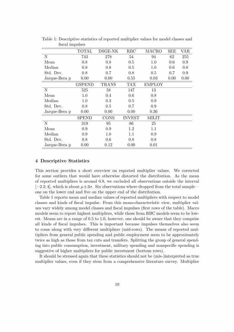
Table 1: Descriptive statistics of reported multiplier values for model classes andfiscal impulses

TOTAL DSGE-NK RBC MACRO SEE VARN 743 278 54 94 62 255Mean 0.8 0.8 0.5 1.0 0.6 0.9Median 0.8 0.8 0.5 1.0 0.6 0.8Std. Dev. 0.8 0.7 0.8 0.5 0.7 0.9Jarque-Bera p 0.00 0.00 0.55 0.03 0.00 0.00

GSPEND TRANS TAX EMPLOYN 525 58 147 13Mean 1.0 0.4 0.6 0.8Median 1.0 0.3 0.5 0.9Std. Dev. 0.8 0.5 0.7 0.9Jarque-Bera p 0.00 0.00 0.00 0.36

SPEND CONS INVEST MILITN 319 95 86 25Mean 0.9 0.9 1.2 1.1Median 0.9 1.0 1.1 0.9Std. Dev. 0.8 0.6 0.8 0.8Jarque-Bera p 0.00 0.12 0.00 0.01

4 Descriptive Statistics

This section provides a short overview on reported multiplier values. We correctedfor some outliers that would have otherwise distorted the distribution. As the meanof reported multipliers is around 0.8, we excluded all observations outside the interval[−2.2; 4], which is about µ±3σ. Six observations where dropped from the total sample—one on the lower end and five on the upper end of the distribution.Table 1 reports mean and median values of reported multipliers with respect to model

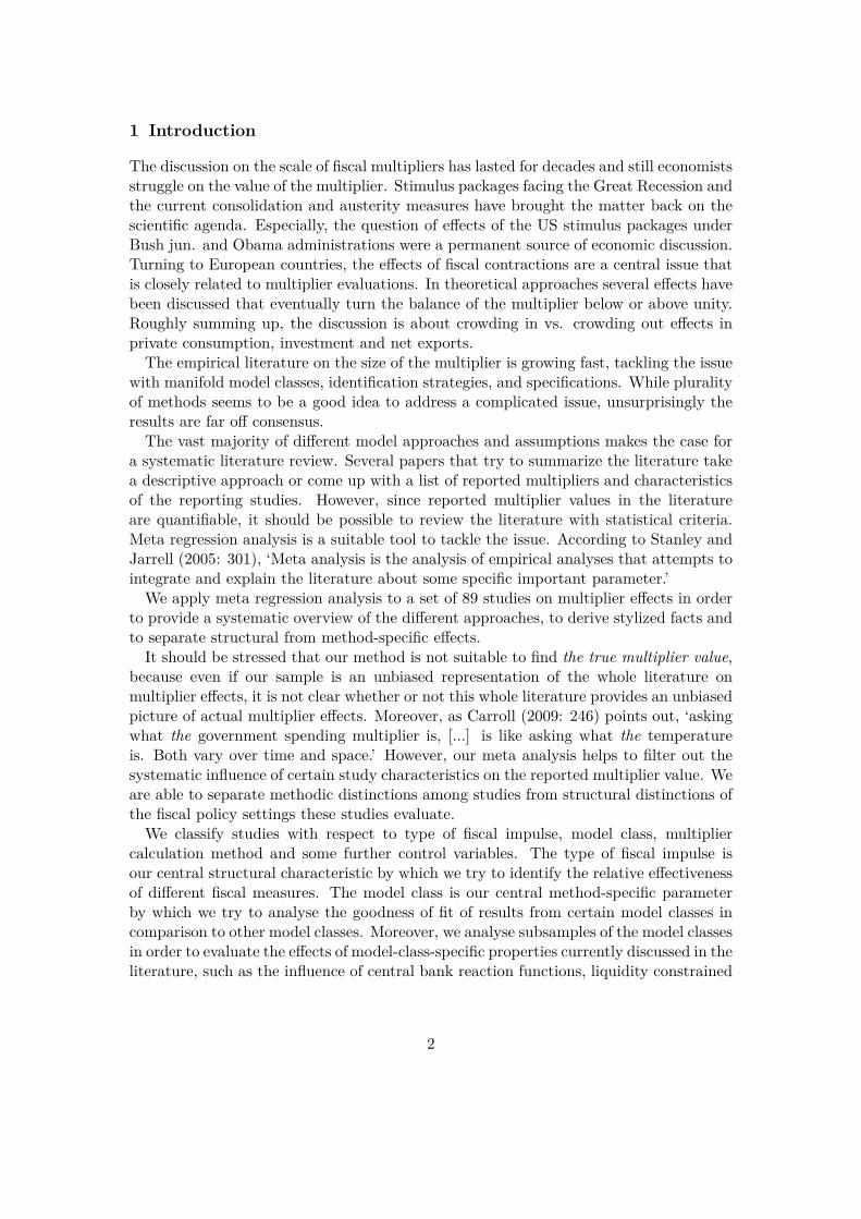
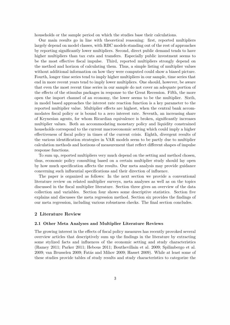
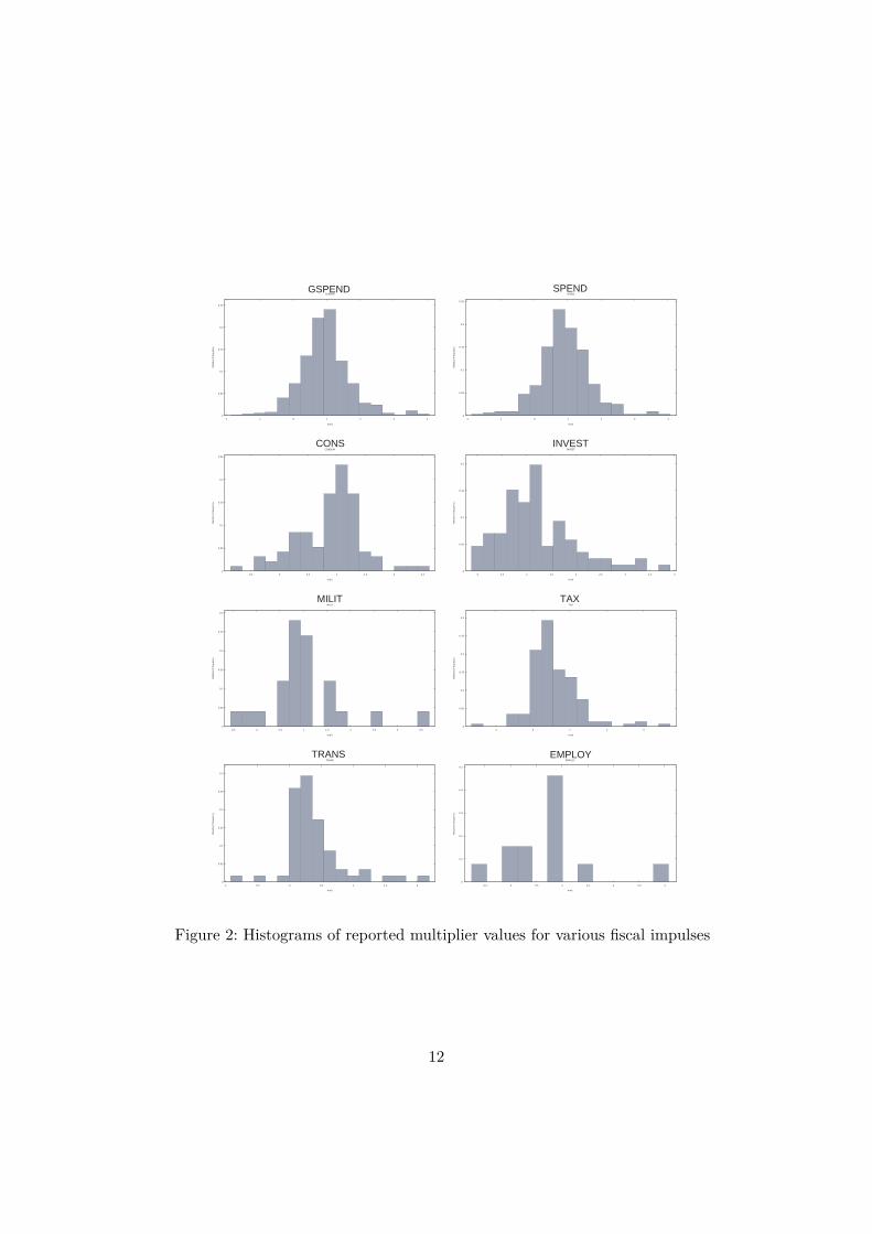
classes and kinds of fiscal impulse. From this mono-characteristic view, multiplier val-ues vary widely among model classes and fiscal impulses (first rows of the table). Macromodels seem to report highest multipliers, while those from RBC models seem to be low-est. Means are in a range of 0.5 to 1.0, however, one should be aware that they compriseall kinds of fiscal impulses. This is important because impulses themselves also seemto come along with very different multipliers (mid-rows). The means of reported mul-tipliers from general public spending and public employment seem to be approximatelytwice as high as those from tax cuts and transfers. Splitting the group of general spend-ing into public consumption, investment, military spending and nonspecific spending issuggestive of higher multipliers for public investment (bottom rows).It should be stressed again that these statistics should not be (mis-)interpreted as true

multiplier values, even if they stem from a comprehensive literature survey. Multiplier

10

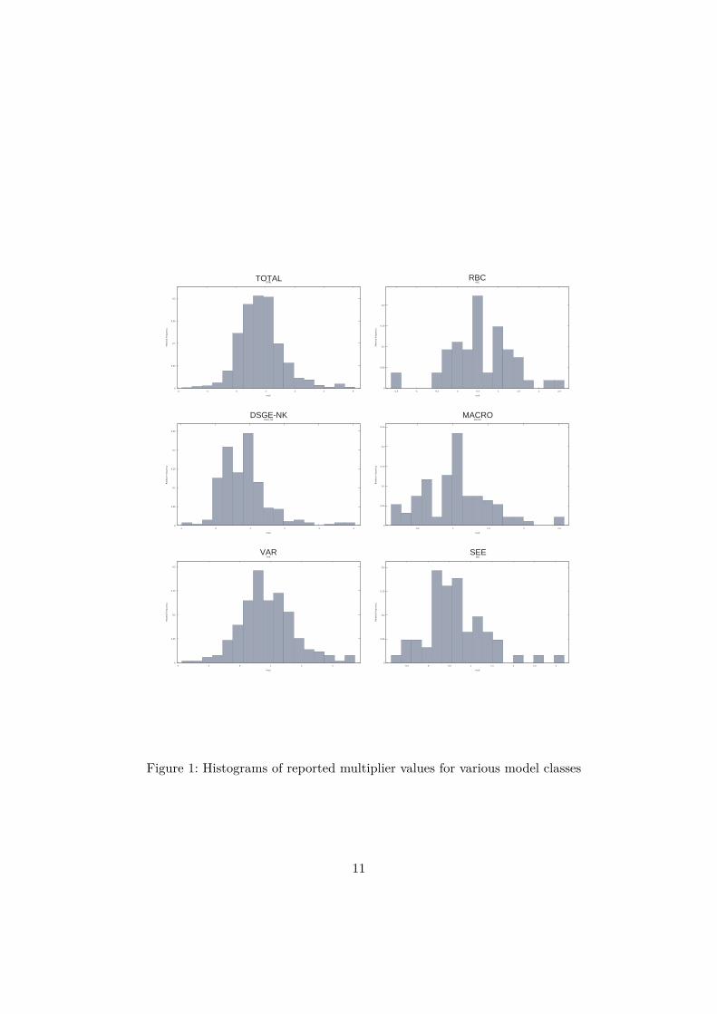
TOTAL RBC

DSGE-NK MACRO

VAR SEE

Figure 1: Histograms of reported multiplier values for various model classes

11

GSPEND SPEND

CONS INVEST

MILIT TAX

TRANS EMPLOY

Figure 2: Histograms of reported multiplier values for various fiscal impulses

12

calculations may all be biased in some direction and several significant influences areunaccounted for at this point. Properties of the distribution should advise caution aswell. Even though means are relatively close to medians for each model class and impulse,Figures 1 and 2 show that multipliers for the subgroups are by and large not normallydistributed, which is confirmed by Jarque-Bera probabilities. Multimodal distributionspoint to additional influential factors. Of course, obvious distortional factors are modelclasses interfering the distributions of fiscal impulses and vice versa, but also the othervariables introduced in the former section should be tested. This is why we perform ameta analysis on our sample. The aim is to separate the influences of model classes andtypes of impulses and to check for additional significant influences.

5 Meta Regression Analysis – Method

For the proposed meta analysis we stick to Stanley and Jarrell (2005: 302). In general,our model reads

kj = κ+ Zjα+ δi + εj j = 1, ..., N i = 1, ...,M (4)

with

• kj multiplier value of observation j

• κ “underlying” or “reference” multiplier value

• Zj vector of characteristics (“moderator variables”) of observation j

• α vector of systematic effects of Zj on kj

• δi vector of paper-specific intercepts (paper dummies)

We include dummies δi for each paper in order to control for paper-specific interceptsand use heteroscedasticity-robust estimators. However, to keep track of the main resultswe do not display the 89 paper dummies in regression tables (results are available onrequest), but we discuss their influence. Some further methodical questions need to beaddressed. Meta studies often use normalisation tools to construct the effect size. To endup with a dimensionless scale, the average outcome of a treatment group is subtractedby the average outcome of the control group divided by standard deviation of the controlgroup (Stanley 2001: 135). Normalisation is not an issue for our purpose, because themultiplier is already dimensionless. On the other hand, as mentioned above, multipliervalues are not measured in a standardised manner. We control for the multiplier cal-culation method and the time horizon to extract comparable multiplier values, but itshould be pointed out that this may only be a second best solution. However, there is noestablished method to translate, for example, peak multipliers into integral multipliers,or a multiplier for a horizon of ten quarters into a multiplier for five quarters.According to Goldfarb and Stekler (2002), a general problem is double counting when

several meta studies use the same data base (for instance US quarterly data from 1970-2005). Meta analysis should include only distinct and separate observations and not

13

clones or reiterations of existing studies. However, for our purpose the same data setdoes not imply the same study setup. One data set can be used with different methodsand model classes. These different approaches help to discriminate between specificationsand should thus be included entirely.A different question is whether to include multiple observations from one study, e. g.

when the authors deal with various models, countries or types of fiscal impulse. Stanley(2001: 138) suggests to use only one observation per study or to take the average in orderto control for undue weight of a single study. While this is a reasonable claim, thereare some important counter-arguments. First, there is a clear trade-off with variabilityand degrees of freedom. Second, when picking only one observation per study, the metaanalyser must take a tough decision, which one to include. Third, taking the averagevalue may be possible for the reported multipliers, yet this technique is not valid for studycharacteristics of a nominal (categorical) scale type, such as the type of fiscal impulse.Fourth, taking only one observation from a comprehensive study may likewise give anundue weight to less-comprehensive studies. We and also other authors (De Grauweand Costa Storti 2004; Nijkamp and Poot 2004; Card et al. 2010; Rusnák et al. 2011)therefore prefer including more than one observation per study. This method has beentested superior to picking only single observations per paper (Bijmolt and Pieters 2001).By using dummies for each paper, the specialty of a study is controlled for to a certaindegree.Nevertheless, we are aware of the problem of over-weighing, and thus check the ro-

bustness of our results in several ways. First, we exclude single papers with manyobservations (N ≥ 30) from our sample. Second, for the total sample, we perform arobustness check by taking only one observation per study into account, namely themedian value. Third, following (Sethuraman 1995), for each (sub-)sample we set up aweighted sample, by weighting each observation of a paper by the number of observationsin the paper; that is, given a paper reports five different multiplier estimates, we includeevery estimate weighted by 1/5. The same technique applies to the study characteris-tics. In total every study is equally weighted. By doing so, we strike a balance betweenproportional influence of single studies versus degrees of freedom and variability in oursurvey. The resulting estimates for α are weighted least squares estimators. Results ofthese robustness checks can be found in the appendix.Other meta studies differentiate the quality of included studies. Stanley (1998), for

example, checks for quality on the basis of degrees of freedom, number of robustnesstests and thus the number of different specifications of an included study; a higher num-ber of degrees of freedom and different specifications should hint at a better diagnosis.De Grauwe and Costa Storti (2004) use the sample size as a quality weight. We do notperform quality selections for our total sample because the above mentioned criteria arenot suitable for model-based approaches. However, for the subsamples on VAR and SEEthe length and the frequency of the time series could provide information on quality.A usual exercise for meta analyses is to control for a possible publication bias, i. e. the

preference for statistically significant results in publication selection (Stanley 2008). Wedo not perform such a test for several reasons. First, our data set does not allow for stateof the art tests of publication bias via funnel asymmetry testing or meta significance

14

testing because RBC, DSGE and MACRO models do not produce standard errors oftheir results, which are necessary to apply these publication bias tests. Second, we couldeasily apply the more straightforward approach of Card et al. (2010), who simply setup a dummy for published versus unpublished studies. We are not convinced of thismethod for our purpose because we could only distinguish between journal publications(published) and working papers (unpublished). This distinction, however, is not clearcut, since major working paper series employ a refereeing process. Moreover, workingpapers in general are close to publication and their results have often undergone aninternal publication selection by the authors. Third and most striking, after scanningthe literature we do not expect a systematic preference for significant positive or negativemultipliers. The aim of most of the studies is simply to calculate multiplier values,irrespective of their significance levels against zero.

6 Meta Regression Analysis – Results

In this section we present and discuss our results. For convenience, Table 2 lists thecharacteristics we tested for.First, we regress reported multipliers of the total sample on characteristics as shown

in Table 3. Groups of variables measured on a nominal scale, such as model class ortype of impulse, are necessarily multicollinear because any observation must belong toexactly one value in this group. That is why one variable of a closed group is omitted.The influence of these omitted variables is reflected in the constant (κ), which is thuscalled reference value. It now becomes clear that κ should not be interpreted as the truemultiplier because it depends on the reference specification.Since we use dummies for each paper, again one of the dummies is omitted due to

exact collinearity and its influence on the dependent variable is thus reflected in κ. Inorder to avoid a bias of the paper dummies on κ, we ran two stages of each regression.In a first step, we included all paper dummies, let the econometric software randomlychoose the paper dummy to drop and calculated the mean coefficient of paper dummies.In a second step, we manually dropped the dummy closest to this mean and thereforeget a reference value with a minimized bias from paper dummies. It should be pointedout that the choice of the omitted paper dummy in no way influences any of the othercharacteristics, but only shifts the reference value κ.The reference for the prime estimation in column (1) is an average multiplier value

calculated as an integral response to an unspecified public spending impulse, stemmingfrom a largely estimated RBCmodel. Such an observation on average reports a multiplierof close to zero when controlling for other influences, which is not significantly differentfrom zero.Fiscal impulses differ significantly concerning their influence on the multiplier. Es-

pecially public investment produces higher multiplier values in our data set, while taxcuts and transfers have a significantly lower impact compared to direct public spending.For military spending and public employment there is only an insignificant difference tounspecified public spending.

15

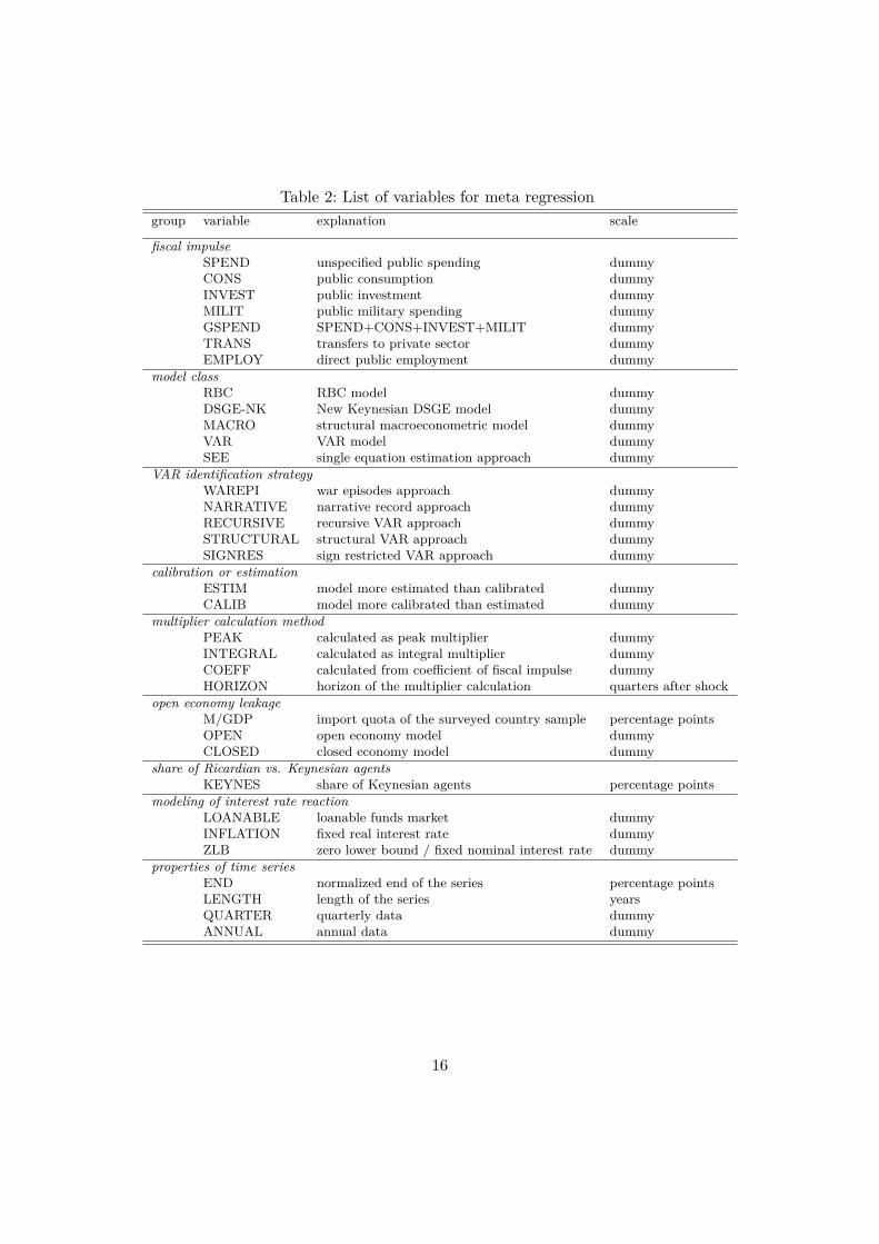
Table 2: List of variables for meta regressiongroup variable explanation scale

fiscal impulseSPEND unspecified public spending dummyCONS public consumption dummyINVEST public investment dummyMILIT public military spending dummyGSPEND SPEND+CONS+INVEST+MILIT dummyTRANS transfers to private sector dummyEMPLOY direct public employment dummy

model classRBC RBC model dummyDSGE-NK New Keynesian DSGE model dummyMACRO structural macroeconometric model dummyVAR VAR model dummySEE single equation estimation approach dummy

VAR identification strategyWAREPI war episodes approach dummyNARRATIVE narrative record approach dummyRECURSIVE recursive VAR approach dummySTRUCTURAL structural VAR approach dummySIGNRES sign restricted VAR approach dummy

calibration or estimationESTIM model more estimated than calibrated dummyCALIB model more calibrated than estimated dummy

multiplier calculation methodPEAK calculated as peak multiplier dummyINTEGRAL calculated as integral multiplier dummyCOEFF calculated from coefficient of fiscal impulse dummyHORIZON horizon of the multiplier calculation quarters after shock

open economy leakageM/GDP import quota of the surveyed country sample percentage pointsOPEN open economy model dummyCLOSED closed economy model dummy

share of Ricardian vs. Keynesian agentsKEYNES share of Keynesian agents percentage points

modeling of interest rate reactionLOANABLE loanable funds market dummyINFLATION fixed real interest rate dummyZLB zero lower bound / fixed nominal interest rate dummy

properties of time seriesEND normalized end of the series percentage pointsLENGTH length of the series yearsQUARTER quarterly data dummyANNUAL annual data dummy

16

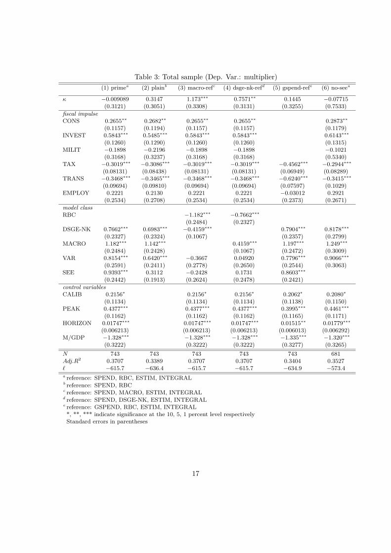
Table 3: Total sample (Dep. Var.: multiplier)(1) primea (2) plainb (3) macro-refc (4) dsge-nk-refd (5) gspend-refe (6) no-seea

κ −0.009089 0.3147 1.173∗∗∗ 0.7571∗∗ 0.1445 −0.07715(0.3121) (0.3051) (0.3308) (0.3131) (0.3255) (0.7533)

fiscal impulseCONS 0.2655∗∗ 0.2682∗∗ 0.2655∗∗ 0.2655∗∗ 0.2873∗∗

(0.1157) (0.1194) (0.1157) (0.1157) (0.1179)INVEST 0.5843∗∗∗ 0.5485∗∗∗ 0.5843∗∗∗ 0.5843∗∗∗ 0.6143∗∗∗

(0.1260) (0.1290) (0.1260) (0.1260) (0.1315)MILIT −0.1898 −0.2196 −0.1898 −0.1898 −0.1021

(0.3168) (0.3237) (0.3168) (0.3168) (0.5340)TAX −0.3019∗∗∗ −0.3086∗∗∗ −0.3019∗∗∗ −0.3019∗∗∗ −0.4562∗∗∗ −0.2944∗∗∗

(0.08131) (0.08438) (0.08131) (0.08131) (0.06949) (0.08289)TRANS −0.3468∗∗∗ −0.3465∗∗∗ −0.3468∗∗∗ −0.3468∗∗∗ −0.6240∗∗∗ −0.3415∗∗∗

(0.09694) (0.09810) (0.09694) (0.09694) (0.07597) (0.1029)EMPLOY 0.2221 0.2130 0.2221 0.2221 −0.03012 0.2921

(0.2534) (0.2708) (0.2534) (0.2534) (0.2373) (0.2671)model classRBC −1.182∗∗∗ −0.7662∗∗∗

(0.2484) (0.2327)DSGE-NK 0.7662∗∗∗ 0.6983∗∗∗ −0.4159∗∗∗ 0.7904∗∗∗ 0.8178∗∗∗

(0.2327) (0.2324) (0.1067) (0.2357) (0.2799)MACRO 1.182∗∗∗ 1.142∗∗∗ 0.4159∗∗∗ 1.197∗∗∗ 1.249∗∗∗

(0.2484) (0.2428) (0.1067) (0.2472) (0.3009)VAR 0.8154∗∗∗ 0.6420∗∗∗ −0.3667 0.04920 0.7796∗∗∗ 0.9066∗∗∗

(0.2591) (0.2411) (0.2778) (0.2650) (0.2544) (0.3063)SEE 0.9393∗∗∗ 0.3112 −0.2428 0.1731 0.8603∗∗∗

(0.2442) (0.1913) (0.2624) (0.2478) (0.2421)control variablesCALIB 0.2156∗ 0.2156∗ 0.2156∗ 0.2062∗ 0.2080∗

(0.1134) (0.1134) (0.1134) (0.1138) (0.1150)PEAK 0.4377∗∗∗ 0.4377∗∗∗ 0.4377∗∗∗ 0.3995∗∗∗ 0.4461∗∗∗

(0.1162) (0.1162) (0.1162) (0.1165) (0.1171)HORIZON 0.01747∗∗∗ 0.01747∗∗∗ 0.01747∗∗∗ 0.01515∗∗ 0.01779∗∗∗

(0.006213) (0.006213) (0.006213) (0.006013) (0.006292)M/GDP −1.328∗∗∗ −1.328∗∗∗ −1.328∗∗∗ −1.335∗∗∗ −1.320∗∗∗

(0.3222) (0.3222) (0.3222) (0.3277) (0.3265)N 743 743 743 743 743 681Adj.R2 0.3707 0.3389 0.3707 0.3707 0.3404 0.3527` −615.7 −636.4 −615.7 −615.7 −634.9 −573.4a reference: SPEND, RBC, ESTIM, INTEGRALb reference: SPEND, RBCc reference: SPEND, MACRO, ESTIM, INTEGRALd reference: SPEND, DSGE-NK, ESTIM, INTEGRALe reference: GSPEND, RBC, ESTIM, INTEGRAL*, **, *** indicate significance at the 10, 5, 1 percent level respectivelyStandard errors in parentheses

17

The next rows show the influences of other model classes, which are all significantlyhigher than for the RBC specification. Of the four alternative model classes, DSGE-NKmodels tend to report the lowest multipliers, while MACRO models are on the upperend of the scale.Attention should be given to control variables. Calibrated models tend to report higher

multipliers than estimated ones. Estimated models were chosen as reference in order tobetter compare the estimated variants of DSGE and RBC models to MACRO, VARand SEE approaches, which are estimated by nature. Peak multipliers are, as expected,significantly higher than integral multipliers. A longer horizon of measurement comesalong with higher multipliers. Import quotas are highly significant with a negativeimpact on reported multipliers.To do some first robustness checks, we estimated some variants of the regression in

column (1). Column (2) shows a plain model without control variables. Results of ourprime model are reconfirmed by and large. However, excluding control variables increasesthe reference multiplier and renders the difference between RBC and SEE approachesinsignificant. A stepwise exclusion of controls shows that both effects largely dependon the inclusion of PEAK. This is reasonable given that peak multipliers are signifi-cantly higher and that single equation estimations cannot be differentiated with respectto peak or integral multipliers. Not controlling for this difference shifts the referencemultiplier upwards and SEE multipliers downwards relative to all other model classes.The stepwise exclusion of control variables does not affect the other controls except forHORIZON that becomes insignificant when excluding PEAK. This effect is coherentwith our reasoning that peak multipliers are usually recorded on a shorter horizon thanintegral multipliers. Ignoring the heterogeneity of peak and integral multipliers obscuresthe specific information of HORIZON.The regression model in column (3) tests the impact of exchanging the reference

model class. Using observations from MACRO models as reference only affects theconstant and the model class group. The test reveals that DSGE-NK and RBC modelsreport significantly lower multipliers, while VAR and SEE do not. When DSGE-NKmodels serve as reference, as shown in column (4), VAR and SEE coefficients are alsoinsignificant, while the coefficent for RBC is significantly lower and the one for MACROmodels is significantly higher. Taking all these information together, DSGE-NK andMACRO models are close to the more data based VAR and SEE approaches, whileRBC models negatively stand out of the model classes tested.Column (5) shows that our results are robust to a different reference fiscal impulse

(GSPEND), where we do not distinguish public spending, consumption, investment andmilitary spending. Coefficients and significance levels are only altered very slightly incomparison to column (1).Since SEE multipliers are calculated in a different way compared to those of other

model classes, in column (6) we test the robustness of our results when excluding obser-vations from SEE models. There is almost no change in coefficients from this exercise.The total sample comprised both model based approaches and empirical approaches,

which could be criticized for comparing apples with oranges. However, both methodsare coequally used for policy consulting and the meta regressions on the total sample

18

mark their potential differences.We now turn to subsamples in order to perform some additional robustness tests and

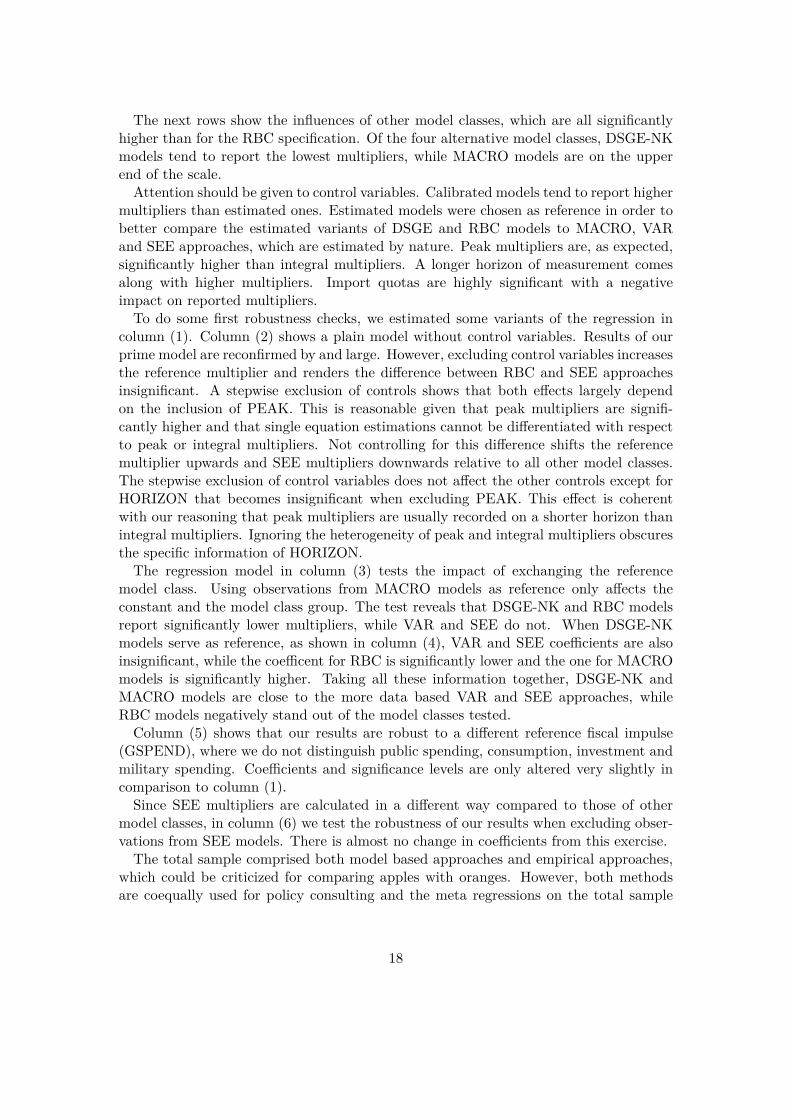
to control for characteristics that apply to specific model classes only. We start withsubsample#I, comprising observations from model based approaches (RBC, DSGE-NK,MACRO). Regression results are shown in Table 4, which provides the prime regressionfor this subsample as well as some simple robustness checks akin to the ones in Table 3.Most results of the total sample are reaffirmed with subsample#I. The reference value

is not significantly different from zero. Concerning fiscal impulses, public investmentstill significantly increases the reported multiplier, while tax cuts and transfers decreaseit. Unlike the total sample, in subsample#I military spending induces the strongestmultiplier effects.Model classes differ significantly with highest value for MACRO models. Exchanging

the reference model class, as done in column (4), where a DSGE-NK models serves asreference instead of a RBC model, does not alter the results for other characteristics,but reveals the difference between DSGE-NK and MACRO models insignificant for thisspecification.The additional characteristics concerning agent behavior, interest rate reaction and

openness to trade are all significant. As expected, the higher the share of Keynesianagents, the higher the reported multiplier. Comparing columns (1) and (2) shows thatdropping additional characteristics, and thus testing the same characteristics as for thetotal sample, restores the significant distance between MACRO and DSGE-NK multi-pliers, which appeared in the total sample. Stepwise exclusion of additional character-istics reveals that agent behavior largely accounts for this difference. In other words,New Keynesian DSGE models without Ricardian agents produce insignificantly differentmultiplier effects as compared to structural macro models where Ricardian Equivalencedoes not apply in general.Models with a loanable funds specification of the interest rate, which is our reference

here, tend to have the lowest multipliers. Including a central bank reaction function withan inflation target significantly increases the multiplier. This is pretty much the samefor models with a fixed real rate of interest. The highest multipliers result from modelswith a zero lower bound specification. When a model with a fixed real rate of interestserves as reference (column (6)), it can be shown that models with inflation targetingdo not significantly differ, while the ZLB specification is still significantly higher. Otherregression coefficients are unaffected by this modification. Open-economy models pointto lower multipliers than closed-economy models.The other control variables have the same algebraic sign as compared to the total

sample. However, they are not significant, except for the import quota. Setting up plainregressions without control variables and additional characteristics (columns (3) and (4))does not alter the results qualitatively.Meta regression results for subsample#II, which is akin to subsample#I, but focuses

on RBC and DSGE-NK models only, are displayed in Table 5. Subsample#II is actuallya mere robustness check to #I because the same characteristics are tested. There areonly some slight distinctions: it is no use to test for other reference models since thereare only two possible model classes. Concerning the interest rate reaction function,

19

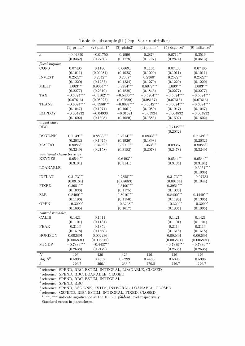
Table 4: subsample#I (Dep. Var.: multiplier)(1) primea (2) plain1b (3) plain2c (4) plain3d (5) dsge-refe (6) intfix-reff

κ −0.04350 −0.01750 0.1996 0.2873 0.6714∗∗ 0.3516(0.3462) (0.2760) (0.1778) (0.1797) (0.2874) (0.3613)

fiscal impulseCONS 0.07406 0.1180 0.06691 0.1104 0.07406 0.07406

(0.1011) (0.09981) (0.1023) (0.1009) (0.1011) (0.1011)INVEST 0.2522∗∗ 0.2542∗∗ 0.2337∗ 0.2360∗ 0.2522∗∗ 0.2522∗∗

(0.1220) (0.1257) (0.1234) (0.1270) (0.1220) (0.1220)MILIT 1.003∗∗∗ 0.9064∗∗∗ 0.8954∗∗∗ 0.8077∗∗∗ 1.003∗∗∗ 1.003∗∗∗

(0.2277) (0.2319) (0.1828) (0.1846) (0.2277) (0.2277)TAX −0.5324∗∗∗ −0.5102∗∗∗ −0.5436∗∗∗ −0.5204∗∗∗ −0.5324∗∗∗ −0.5324∗∗∗

(0.07616) (0.08027) (0.07820) (0.08157) (0.07616) (0.07616)TRANS −0.6024∗∗∗ −0.5986∗∗∗ −0.6087∗∗∗ −0.6042∗∗∗ −0.6024∗∗∗ −0.6024∗∗∗

(0.1047) (0.1071) (0.1061) (0.1080) (0.1047) (0.1047)EMPLOY −0.004832 −0.04930 −0.01681 −0.05924 −0.004832 −0.004832

(0.1602) (0.1508) (0.1680) (0.1585) (0.1602) (0.1602)model classRBC −0.7149∗∗∗

(0.2032)DSGE-NK 0.7149∗∗∗ 0.8833∗∗∗ 0.7214∗∗∗ 0.8833∗∗∗ 0.7149∗∗∗

(0.2032) (0.1975) (0.1926) (0.1898) (0.2032)MACRO 0.8086∗∗ 1.349∗∗∗ 0.8271∗∗∗ 1.353∗∗∗ 0.09367 0.8086∗∗

(0.3249) (0.2158) (0.3182) (0.2078) (0.2478) (0.3249)additional characteristicsKEYNES 0.6544∗∗ 0.6493∗∗ 0.6544∗∗ 0.6544∗∗

(0.3184) (0.3141) (0.3184) (0.3184)LOANABLE −0.3951∗∗∗

(0.1036)INFLAT 0.3173∗∗∗ 0.2855∗∗∗ 0.3173∗∗∗ −0.07782

(0.09164) (0.08683) (0.09164) (0.1044)FIXED 0.3951∗∗∗ 0.3190∗∗∗ 0.3951∗∗∗

(0.1036) (0.1175) (0.1036)ZLB 0.8400∗∗∗ 0.8010∗∗∗ 0.8400∗∗∗ 0.4449∗∗∗

(0.1196) (0.1150) (0.1196) (0.1305)OPEN −0.3299∗ −0.3298∗∗ −0.3299∗ −0.3299∗

(0.1805) (0.1617) (0.1805) (0.1805)control variablesCALIB 0.1421 0.1611 0.1421 0.1421

(0.1101) (0.1131) (0.1101) (0.1101)PEAK 0.2113 0.1859 0.2113 0.2113

(0.1518) (0.1668) (0.1518) (0.1518)HORIZON 0.002891 0.002236 0.002891 0.002891

(0.005891) (0.006317) (0.005891) (0.005891)M/GDP −0.7339∗∗∗ −0.4437∗∗ −0.7339∗∗∗ −0.7339∗∗∗

(0.2638) (0.2179) (0.2638) (0.2638)N 426 426 426 426 426 426Adj.R2 0.5396 0.4537 0.5299 0.4483 0.5396 0.5396` −226.7 −266.1 −233.5 −270.5 −226.7 −226.7a reference: SPEND, RBC, ESTIM, INTEGRAL, LOANABLE, CLOSEDb reference: SPEND, RBC, LOANABLE, CLOSEDc reference: SPEND, RBC, ESTIM, INTEGRALd reference: SPEND, RBCe reference: SPEND, DSGE-NK, ESTIM, INTEGRAL, LOANABLE, CLOSEDf reference: GSPEND, RBC, ESTIM, INTEGRAL, FIXED, CLOSED*, **, *** indicate significance at the 10, 5, 1 percent level respectivelyStandard errors in parentheses

20

there is no observation with a fixed real rate of interest for this sample, which is whythe variable is dropped. Notwithstanding these slight distinctions, Table 5 by and largereproduces the results from Table 4, except for the inflation target specification, which isnow insignificantly different from a loanable funds specification. However, models with azero lower bound setting still produce significantly higher multipliers. The high effect ofmilitary spending compared to spending in general seems to be a special characteristicof model based approaches, since this is not confirmed by the total sample and thefollowing subsamples.With subsample#III, which takes into account observations from MACRO, VAR and

SEE approaches, the complement to subsample#II is tested. Results are shown in Table6. Due to heterogeneity of the model classes, we simply test for the broad characteristicsof the total sample, omitting the calibration vs. estimation dummy that does not applyfor this group because all of them are estimated. Regression results in all four columnsare qualitatively similar to those of the total sample. Public investment seems to bethe most effective fiscal impulse in our sample. Indirect impulses, such as taxes andtransfers, seem to be less effective, although results are less significant, probably due tothe smaller sample size. Military spending turns insignificant again. The three modelclasses do not produce significantly different multipliers.Control variables show the same pattern as in Table 3. The high significance levels

of multiplier calculation method and horizon that appeared in the total sample seem tohave their roots in VAR and SEE approaches, since they do not appear in subsamples #Iand #II. This is perfectly in line with intuition because the IRFs of the more model-basedapproaches are much smoother.Subsample#IV focuses on VAR and SEE approaches only. It is thus the complement

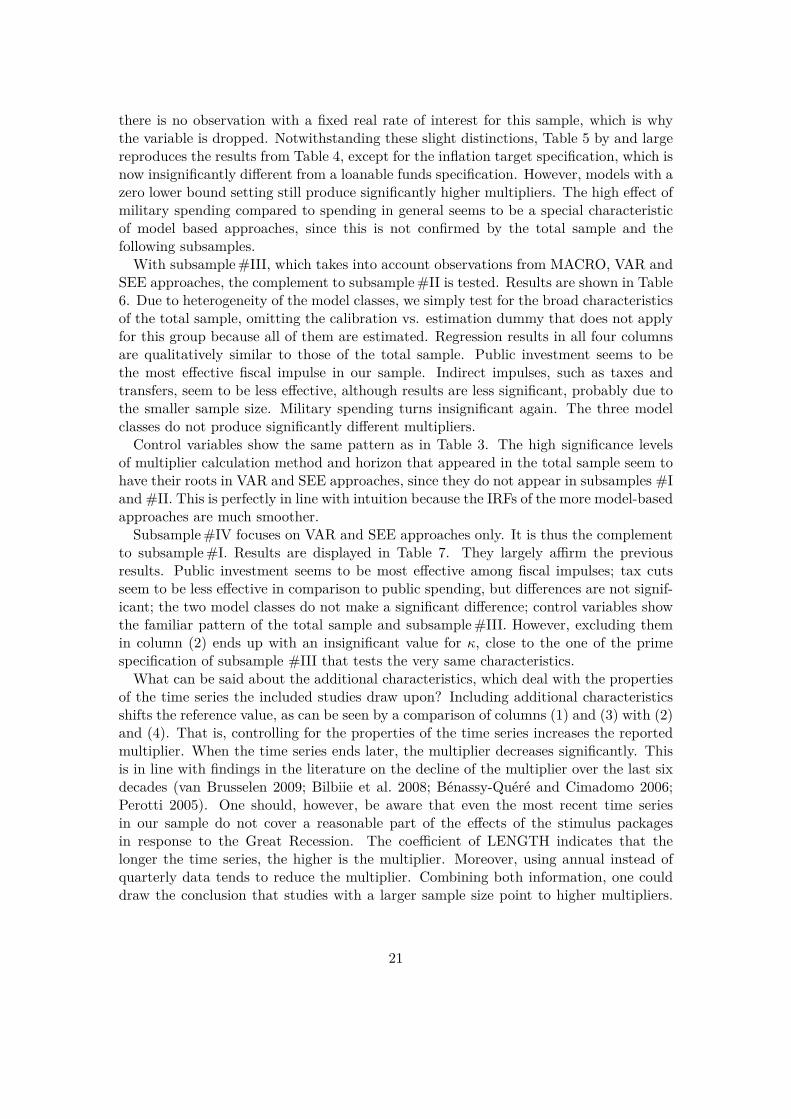
to subsample#I. Results are displayed in Table 7. They largely affirm the previousresults. Public investment seems to be most effective among fiscal impulses; tax cutsseem to be less effective in comparison to public spending, but differences are not signif-icant; the two model classes do not make a significant difference; control variables showthe familiar pattern of the total sample and subsample#III. However, excluding themin column (2) ends up with an insignificant value for κ, close to the one of the primespecification of subsample #III that tests the very same characteristics.What can be said about the additional characteristics, which deal with the properties

of the time series the included studies draw upon? Including additional characteristicsshifts the reference value, as can be seen by a comparison of columns (1) and (3) with (2)and (4). That is, controlling for the properties of the time series increases the reportedmultiplier. When the time series ends later, the multiplier decreases significantly. Thisis in line with findings in the literature on the decline of the multiplier over the last sixdecades (van Brusselen 2009; Bilbiie et al. 2008; Bénassy-Quéré and Cimadomo 2006;Perotti 2005). One should, however, be aware that even the most recent time seriesin our sample do not cover a reasonable part of the effects of the stimulus packagesin response to the Great Recession. The coefficient of LENGTH indicates that thelonger the time series, the higher is the multiplier. Moreover, using annual instead ofquarterly data tends to reduce the multiplier. Combining both information, one coulddraw the conclusion that studies with a larger sample size point to higher multipliers.

21

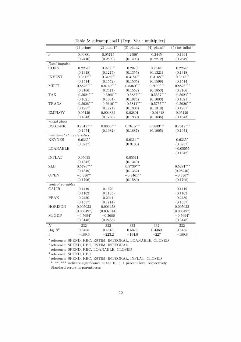
Table 5: subsample#II (Dep. Var.: multiplier)(1) primea (2) plain1b (3) plain2c (4) plain3d (5) int-inflate

κ 0.09881 0.05715 0.2590∗ 0.2445 0.1494(0.2416) (0.2809) (0.1493) (0.2212) (0.2649)

fiscal impulseCONS 0.2254∗ 0.2700∗∗ 0.2070 0.2548∗ 0.2254∗

(0.1318) (0.1275) (0.1355) (0.1321) (0.1318)INVEST 0.3517∗∗ 0.3459∗∗ 0.3184∗∗ 0.3168∗∗ 0.3517∗∗

(0.1514) (0.1552) (0.1565) (0.1599) (0.1514)MILIT 0.8826∗∗∗ 0.8769∗∗∗ 0.8360∗∗∗ 0.8077∗∗∗ 0.8826∗∗∗

(0.2166) (0.2471) (0.1552) (0.1853) (0.2166)TAX −0.5624∗∗∗ −0.5368∗∗∗ −0.5837∗∗∗ −0.5557∗∗∗ −0.5624∗∗∗

(0.1021) (0.1034) (0.1074) (0.1083) (0.1021)TRANS −0.5626∗∗∗ −0.5610∗∗∗ −0.5811∗∗∗ −0.5755∗∗∗ −0.5626∗∗∗

(0.1257) (0.1271) (0.1308) (0.1319) (0.1257)EMPLOY 0.05129 0.004835 0.02801 −0.01318 0.05129

(0.1843) (0.1738) (0.1939) (0.1836) (0.1843)model classDSGE-NK 0.7612∗∗∗ 0.8833∗∗∗ 0.7615∗∗∗ 0.8833∗∗∗ 0.7612∗∗∗

(0.1974) (0.1982) (0.1887) (0.1905) (0.1974)additional characteristicsKEYNES 0.6335∗ 0.6314∗∗ 0.6335∗

(0.3237) (0.3185) (0.3237)LOANABLE −0.05055

(0.1342)INFLAT 0.05055 0.05511

(0.1342) (0.1349)ZLB 0.5786∗∗∗ 0.5739∗∗∗ 0.5281∗∗∗

(0.1349) (0.1352) (0.08240)OPEN −0.3367∗ −0.3461∗∗ −0.3367∗

(0.1796) (0.1580) (0.1796)control variablesCALIB 0.1419 0.1629 0.1419

(0.1102) (0.1135) (0.1102)PEAK 0.2430 0.2041 0.2430

(0.1557) (0.1714) (0.1557)HORIZON 0.005032 0.003458 0.005032

(0.006497) (0.007014) (0.006497)M/GDP −0.5694∗ −0.3686 −0.5694∗

(0.3148) (0.2485) (0.3148)N 332 332 332 332 332Adj.R2 0.5455 0.4515 0.5375 0.4469 0.5455` −189.6 −223.2 −194.9 −227 −189.6a reference: SPEND, RBC, ESTIM, INTEGRAL, LOANABLE, CLOSEDb reference: SPEND, RBC, ESTIM, INTEGRALc reference: SPEND, RBC, LOANABLE, CLOSEDd reference: SPEND, RBCe reference: SPEND, RBC, ESTIM, INTEGRAL, INFLAT, CLOSED*, **, *** indicate significance at the 10, 5, 1 percent level respectivelyStandard errors in parentheses

22

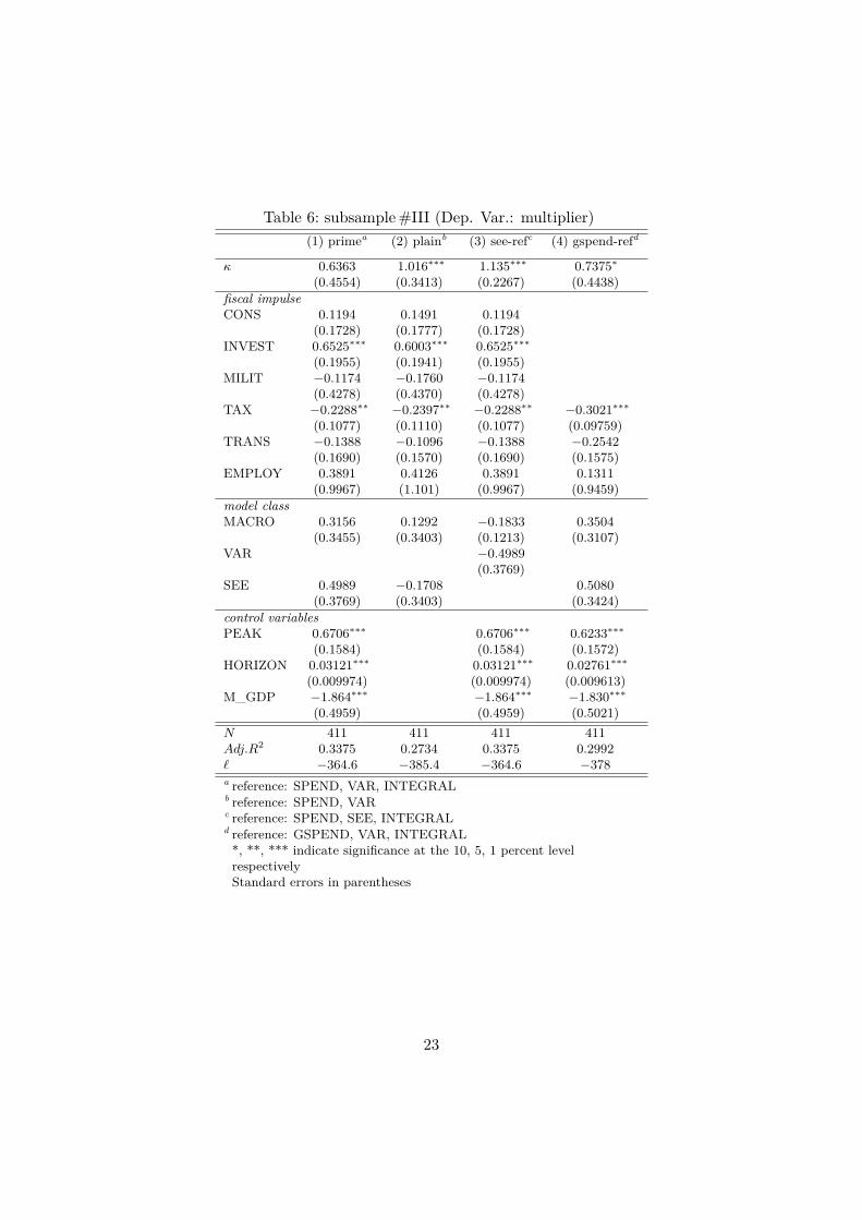
Table 6: subsample#III (Dep. Var.: multiplier)(1) primea (2) plainb (3) see-refc (4) gspend-refd

κ 0.6363 1.016∗∗∗ 1.135∗∗∗ 0.7375∗(0.4554) (0.3413) (0.2267) (0.4438)

fiscal impulseCONS 0.1194 0.1491 0.1194

(0.1728) (0.1777) (0.1728)INVEST 0.6525∗∗∗ 0.6003∗∗∗ 0.6525∗∗∗

(0.1955) (0.1941) (0.1955)MILIT −0.1174 −0.1760 −0.1174

(0.4278) (0.4370) (0.4278)TAX −0.2288∗∗ −0.2397∗∗ −0.2288∗∗ −0.3021∗∗∗

(0.1077) (0.1110) (0.1077) (0.09759)TRANS −0.1388 −0.1096 −0.1388 −0.2542

(0.1690) (0.1570) (0.1690) (0.1575)EMPLOY 0.3891 0.4126 0.3891 0.1311

(0.9967) (1.101) (0.9967) (0.9459)model classMACRO 0.3156 0.1292 −0.1833 0.3504

(0.3455) (0.3403) (0.1213) (0.3107)VAR −0.4989

(0.3769)SEE 0.4989 −0.1708 0.5080

(0.3769) (0.3403) (0.3424)control variablesPEAK 0.6706∗∗∗ 0.6706∗∗∗ 0.6233∗∗∗

(0.1584) (0.1584) (0.1572)HORIZON 0.03121∗∗∗ 0.03121∗∗∗ 0.02761∗∗∗

(0.009974) (0.009974) (0.009613)M_GDP −1.864∗∗∗ −1.864∗∗∗ −1.830∗∗∗

(0.4959) (0.4959) (0.5021)N 411 411 411 411Adj.R2 0.3375 0.2734 0.3375 0.2992` −364.6 −385.4 −364.6 −378a reference: SPEND, VAR, INTEGRALb reference: SPEND, VARc reference: SPEND, SEE, INTEGRALd reference: GSPEND, VAR, INTEGRAL*, **, *** indicate significance at the 10, 5, 1 percent levelrespectivelyStandard errors in parentheses

23

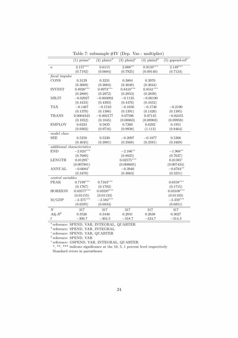
Table 7: subsample#IV (Dep. Var.: multiplier)(1) primea (2) plain1b (3) plain2c (4) plain3d (5) gspend-refe

κ 2.157∗∗∗ 0.6115 2.008∗∗ 0.9133∗∗∗ 2.149∗∗∗(0.7192) (0.6684) (0.7925) (0.09140) (0.7124)

fiscal impulseCONS 0.3129 0.3231 0.3804 0.3970

(0.3009) (0.3004) (0.3048) (0.3044)INVEST 0.8920∗∗∗ 0.8973∗∗∗ 0.8410∗∗∗ 0.8541∗∗∗

(0.2888) (0.2872) (0.2853) (0.2839)MILIT −0.02927 −0.003092 −0.1135 −0.06190

(0.4433) (0.4393) (0.4476) (0.4452)TAX −0.1467 −0.1510 −0.1656 −0.1746 −0.2190

(0.1370) (0.1386) (0.1391) (0.1426) (0.1385)TRANS 0.0004343 −0.002177 0.07596 0.07145 −0.02455

(0.1052) (0.1045) (0.08863) (0.08903) (0.09958)EMPLOY 0.6324 0.5835 0.7260 0.6292 0.1951

(0.9302) (0.9716) (0.9938) (1.113) (0.8464)model classSEE 0.5250 0.5330 −0.2097 −0.1877 0.5306

(0.4045) (0.3981) (0.3568) (0.3591) (0.3469)additional characteristicsEND −2.024∗∗∗ −2.166∗∗ −1.968∗∗

(0.7680) (0.8825) (0.7637)LENGTH 0.01295∗ 0.02575∗∗∗ 0.01385∗

(0.007801) (0.008605) (0.007434)ANNUAL −0.6684∗ −0.3940 −0.6764∗∗

(0.3470) (0.3063) (0.3251)control variablesPEAK 0.7199∗∗∗ 0.7163∗∗∗ 0.6558∗∗∗

(0.1767) (0.1702) (0.1715)HORIZON 0.03577∗∗∗ 0.03597∗∗∗ 0.03108∗∗∗

(0.01155) (0.01133) (0.01103)M/GDP −2.375∗∗∗ −2.582∗∗∗ −2.359∗∗∗

(0.6595) (0.6834) (0.6851)N 317 317 317 317 317Adj.R2 0.3526 0.3446 0.2831 0.2638 0.3027` −300.7 −304.5 −318.7 −324.7 −314.3a reference: SPEND, VAR, INTEGRAL, QUARTERb reference: SPEND, VAR, INTEGRALc reference: SPEND, VAR, QUARTERd reference: SPEND, VARe reference: GSPEND, VAR, INTEGRAL, QUARTER*, **, *** indicate significance at the 10, 5, 1 percent level respectivelyStandard errors in parentheses

24

However, both LENGTH and ANNUAL could carry other information. LENGTH mayalso contain information on the sample period because longer time series on averagereach farther back in time and therefore comprehend periods when multiplier effectswere supposed to be higher. The quarterly vs. annual dummy may be a proxy forprecision, but it may also contain a bias regarding the identification of discretionaryfiscal impulses as discussed for example in Beetsma and Giuliodori (2011: F11). Itshould be pointed out that the coefficients of the other variables are not affected byincluding or excluding the additional variables.We now turn to subsample#V in order to contribute to the discussion on different

identification methods in the VAR literature on fiscal impulses. Results are reportedin Table 8. To start with similarities to other subsamples, again, public investmentseems to be the most effective fiscal impulse. Furthermore, additional characteristicsand control variables are largely in line with those of subsample#IV.The reference value κ is positive and significant throughout most columns. The signifi-

cant values of κ in columns (1), (3), (5) and (6) depend on the inclusion of the additionalcharacteristics, as the plain specifications of column (2) and (4) reveal.As a central issue, the estimation tests the influence of the various identification strate-

gies. The prime specification, including all additional characteristics and control vari-ables shows insignificant differences between identification strategies. They, however,turn significant when excluding control variables in columns (3) and (4). RecursiveVARs, Structural VARs and VARs using the narrative record all seem to have a similarpositive impact on the reported multiplier in comparison to the sign restricted VARsand those based on war episodes. A stepwise inclusion of control variables reveals thatwhether differences are significant or not, depends on the inclusion of PEAK and HORI-ZON, and not on the additional characteristics or the import quota. The impact ofPEAK and HORIZON is not surprising, since the different identification strategies comealong with specific shapes of impulse response functions that are also connected to mul-tiplier calculation method and horizon. Thus, one could conclude that a big part ofthe difference among identification strategies concerning reported multipliers is simply aquestion of timing of measurement. This result is in line with Caldara and Kamps (2008:28); it is confirmed by column (5) because dropping identification strategies even makesa slight increase of the adjusted R2 in comparison to the prime specification. Changingthe reference identification strategy, as in column (6), shifts the reference value and thecoefficients of other identification strategies, but does not alter the other results.Before we conclude, we would like to refer to the statistical appendix that contains

further robustness checks concerning a possible overweighing of comprehensive studies.The columns of Table 9 show results for the prime specification of our total sample, whendropping single papers with many observations (N ≥ 30) from the sample. In Table 10we test weighted versions of the prime specifications of all (sub-)samples by weightingeach observation of a paper by the number of observations in the paper. Finally, Table11 presents alternative specifications of the dependent variable. In column (1) we testa model using only the median multiplier of each study of the total sample. In column(2) and (3) we test a probit and logit model respectively, where the dependent variableis binary, signalling whether the multiplier is greater than or equal to one or whether

25

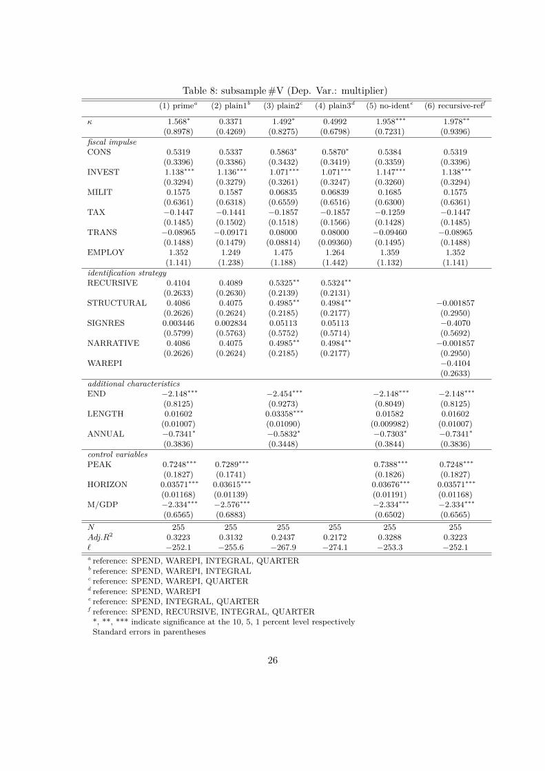
Table 8: subsample#V (Dep. Var.: multiplier)(1) primea (2) plain1b (3) plain2c (4) plain3d (5) no-idente (6) recursive-reff

κ 1.568∗ 0.3371 1.492∗ 0.4992 1.958∗∗∗ 1.978∗∗(0.8978) (0.4269) (0.8275) (0.6798) (0.7231) (0.9396)

fiscal impulseCONS 0.5319 0.5337 0.5863∗ 0.5870∗ 0.5384 0.5319

(0.3396) (0.3386) (0.3432) (0.3419) (0.3359) (0.3396)INVEST 1.138∗∗∗ 1.136∗∗∗ 1.071∗∗∗ 1.071∗∗∗ 1.147∗∗∗ 1.138∗∗∗

(0.3294) (0.3279) (0.3261) (0.3247) (0.3260) (0.3294)MILIT 0.1575 0.1587 0.06835 0.06839 0.1685 0.1575

(0.6361) (0.6318) (0.6559) (0.6516) (0.6300) (0.6361)TAX −0.1447 −0.1441 −0.1857 −0.1857 −0.1259 −0.1447

(0.1485) (0.1502) (0.1518) (0.1566) (0.1428) (0.1485)TRANS −0.08965 −0.09171 0.08000 0.08000 −0.09460 −0.08965

(0.1488) (0.1479) (0.08814) (0.09360) (0.1495) (0.1488)EMPLOY 1.352 1.249 1.475 1.264 1.359 1.352

(1.141) (1.238) (1.188) (1.442) (1.132) (1.141)identification strategyRECURSIVE 0.4104 0.4089 0.5325∗∗ 0.5324∗∗

(0.2633) (0.2630) (0.2139) (0.2131)STRUCTURAL 0.4086 0.4075 0.4985∗∗ 0.4984∗∗ −0.001857

(0.2626) (0.2624) (0.2185) (0.2177) (0.2950)SIGNRES 0.003446 0.002834 0.05113 0.05113 −0.4070

(0.5799) (0.5763) (0.5752) (0.5714) (0.5692)NARRATIVE 0.4086 0.4075 0.4985∗∗ 0.4984∗∗ −0.001857

(0.2626) (0.2624) (0.2185) (0.2177) (0.2950)WAREPI −0.4104

(0.2633)additional characteristicsEND −2.148∗∗∗ −2.454∗∗∗ −2.148∗∗∗ −2.148∗∗∗

(0.8125) (0.9273) (0.8049) (0.8125)LENGTH 0.01602 0.03358∗∗∗ 0.01582 0.01602

(0.01007) (0.01090) (0.009982) (0.01007)ANNUAL −0.7341∗ −0.5832∗ −0.7303∗ −0.7341∗

(0.3836) (0.3448) (0.3844) (0.3836)control variablesPEAK 0.7248∗∗∗ 0.7289∗∗∗ 0.7388∗∗∗ 0.7248∗∗∗

(0.1827) (0.1741) (0.1826) (0.1827)HORIZON 0.03571∗∗∗ 0.03615∗∗∗ 0.03676∗∗∗ 0.03571∗∗∗

(0.01168) (0.01139) (0.01191) (0.01168)M/GDP −2.334∗∗∗ −2.576∗∗∗ −2.334∗∗∗ −2.334∗∗∗

(0.6565) (0.6883) (0.6502) (0.6565)N 255 255 255 255 255 255Adj.R2 0.3223 0.3132 0.2437 0.2172 0.3288 0.3223` −252.1 −255.6 −267.9 −274.1 −253.3 −252.1a reference: SPEND, WAREPI, INTEGRAL, QUARTERb reference: SPEND, WAREPI, INTEGRALc reference: SPEND, WAREPI, QUARTERd reference: SPEND, WAREPIe reference: SPEND, INTEGRAL, QUARTERf reference: SPEND, RECURSIVE, INTEGRAL, QUARTER*, **, *** indicate significance at the 10, 5, 1 percent level respectivelyStandard errors in parentheses

26

it is less than one. The results of all these robustness checks largely affirm our primespecifications.

7 Conclusions

We tested a set of 89 studies on multiplier effects by meta regression analysis in orderto provide a systematic overview of the different approaches, to derive stylized facts andto separate structural from method-specific effects. The method is not suitable to filterout an absolute value for the multiplier, however, it is able to extract relative differencesbetween study characteristics.We now draw a broad picture of our results from the meta analysis. First, reported

multipliers depend on model classes. Controlling for additional variables reveals thatRBC models come up with significantly lower multipliers than the rest of model classes.DSGE-NK models and MACRO models also report significantly different multipliers,however their implications are not significantly different from those of the more dataoriented VAR and SEE approaches.Second, direct public demand tends to have higher multipliers than tax cuts and trans-

fers, even though the difference is not always significant. However, public investmentseems to be the most effective fiscal impulse, a result, which is robust against many spec-ifications. Military spending is preferred solely by the more model based approaches,especially DSGE-NK and RBC models. For VAR and SEE approaches, and for our totalsample, multiplier effects of military spending do not differ from those of public spendingin general.Third, reported multipliers strongly depend on the method and horizon of calculating

them. Peak multipliers are on average greater than integral multipliers and the longerthe horizon of measurement, the higher is the multiplier, even though fiscal impulses arenot permanent. Thus, a simple listing of multiplier values without additional informationon how they were computed could provide a biased picture.Fourth, longer time series and those with a higher frequency tend to imply higher

multipliers in our sample. Time series that end in more recent years tend to imply lowermultipliers. One should, however, be aware that even the most recent time series inour sample do not cover an adequate portion of the effects of the stimulus packages inresponse to the Great Recession.Fifth, the more open the import channel of an economy, the lower seems to be the

multiplier.Sixth, in model based approaches the interest rate reaction function is a key parameter

to the reported multiplier value. Multiplier effects are highest, when the central bank ac-commodates fiscal policy or is bound to a zero interest rate. Seventh, an increasing shareof agents, for whom Ricardian equivalence is broken, significantly increases multipliervalues. Controlling for agent behavior in our sample offsets the difference in reportedmultipliers of New Keynesian DSGE models and structural macro models. Both an ac-commodating monetary policy and liquidity constrained households correspond to thecurrent macroeconomic setting which could imply a higher effectiveness of fiscal policyin times of the current crisis.

27

Eighth, divergent results of the various identification strategies in VAR models seemto be partly due to multiplier calculation methods and horizons of measurement thatreflect different shapes of impulse response functions.As an overall conclusion, we might state that reported multipliers very much depend

on the setting and method chosen. Thus, economic policy consulting based on a certainmultiplier study should lay open by how much specification influences the results. Ourmeta analysis may provide guidance concerning such influential specifications and theirdirection of influence.

References

Ardagna, S. (2001). Fiscal policy composition, public debt, and economic activity. PublicChoice 109, 301–325.

Auerbach, A. J. and Y. Gorodnichenko (2012). Measuring the Output Responses toFiscal Policy. American Economic Journal: Economic Policy (forthcoming).

Baxter, M. and R. G. King (1993). Fiscal policy in general equilibrium. AmericanEconomic Review 83 (3), 315–334.

Beetsma, R. and M. Giuliodori (2011). The Effects of Government Purchases Shocks:Review and Estimates for the EU*. The Economic Journal 121 (550), F4–F32.

Bénassy-Quéré, A. and J. Cimadomo (2006). Changing Patterns of Domestic and Cross-Border Fiscal Policy Multipliers in Europe and the US. CEPII working paper 2006-24.

Bijmolt, T. H. A. and R. G. M. Pieters (2001). Meta-Analysis in Marketing when StudiesContain Multiple Measurements. Marketing Letters 12 (2), 157–169.

Bilbiie, F. O., A. Meier, and G. J. Müller (2008). What Accounts for the Changesin U.S. Fiscal Policy Transmission? Journal of Money, Credit, and Banking 40 (7),1439–1469.

Blanchard, O. and R. Perotti (2002). An Empirical Characterization of the DynamicEffects of Changes in Government Spending and Taxes on Output. Quarterly Journalof Economics 117 (4), 1329–1368.

Bouthevillain, C., J. Caruana, C. Checherita, J. Cunha, E. Gordo, S. Haroutunian,G. Langenus, A. Hubic, B. Manzke, J. J. Pérez, and P. Tommasino (2009). Prosand Cons of various fiscal measures to stimulate the economy. Banque Centrale duLuxembourg working paper 40.

Briotti, M. G. (2005). Economic reactions to public finance: A survey of the literature.European Central Bank occasional paper series 38.

Brückner, M. and A. Tuladhar (2010). Public Investment as a Fiscal Stimulus: Evidencefrom Japan’s Regional Spending During the 1990s. IMF Working Paper WP/10/110.

28

Caldara, D. and C. Kamps (2008). What are the effects of fiscal policy shocks? AVAR-based comparative analysis. European Central Bank working paper series 877.

Card, D., J. Kluve, and A. M. Weber (2010). Active Labour Market Policy Evaluations:A Meta-Analysis. Economic Journal 120, F452–F477.

Card, D. and A. B. Krueger (1995). Time-Series Minimum-Wage Studies: A Meta-analysis. American Economic Review 85 (2), 238–243.

Carroll, C. (2009). Comments and Discussion on ”By How Much Does GDP Rise If theGovernment Buys More Output?”. Brookings Papers on Economic Activity 2009 (2),232–249.

Cwik, T. and V. Wieland (2011). Keynesian government spending multipliers andspillovers in the euro area. Economic Policy 26 (67), 493–549.

De Grauwe, P. and C. Costa Storti (2004). The Effects of Monetary Policy: A Meta-Analysis. CESifo working paper 1224.

Fatás, A. and I. Mihov (2001). The Effects of Fiscal Policy on Consumption and Em-ployment: Theory and Evidence. CEPR Discussion Papers 2760.

Fatás, A. and I. Mihov (2009). Why Fiscal Stimulus is Likely to Work. InternationalFinance 12 (1), 57–73.

Feld, L. P. and J. H. Heckemeyer (2011). FDI and Taxation: A Meta-Study. Journal ofEconomic Surveys 25 (2), 233–272.

Freedman, C., M. Kumhof, D. Laxton, D. Muir, and S. Mursula (2010). Global effectsof fiscal stimulus during the crisis. Journal of Monetary Economics 57 (5), 506–526.

Galí, J., J. D. López-Salido, and J. Vallés (2007). Understanding the Effects of Govern-ment Spending on Consumption. Journal of the European Economic Association 5 (1),227–270.

Goldfarb, R. and H. Stekler (2002). Wheat from Chaff: Meta-Analysis as QuantitativeLiterature Review: Comment. Journal of Economic Perspectives 16 (3), 225–226.

Hasset, K. A. (2009). Why Fiscal Stimulus is Unlikely to Work. International Fi-nance 12 (1), 75–91.

Hebous, S. (2011). The Effects of Discretionary Fiscal Policy on Macroeconomic Aggre-gates: A Reappraisal. Journal of Economic Surveys 25 (4), 674–707.

Linnemann, L. (2006). The Effect of Government Spending on Private Consumption: APuzzle? Journal of Money, Credit, and Banking 38 (7), 1715–1735.

Mazraani, S. (2010). Public Expenditures in an RBC Model: A Likelihood Evaluationof Crowding-in and Crowding-out Effects. Mimeo.

29

Mountford, A. and H. Uhlig (2009). What are the Effects of Fiscal Policy Shocks?Journal of Applied Econometrics 24 (6), 960–992.

Nijkamp, P. and J. Poot (2004). Meta-Analysis of the Effect of Fiscal Policies on Long-Run Growth. European Journal of Political Economy 20 (?), 91–124.

Parker, J. A. (2011). On Measuring the Effects of Fiscal Policy in Recessions. Journalof Economic Literature 49 (3), 703–718.

Perotti, R. (2005). Estimating the effects of fiscal policy in OECD countries. CEPRDiscussion Papers 4842.

Ramey, V. A. (2011). Can Government Purchases Stimulate the Economy? Journal ofEconomic Literature 49 (3), 673–685.

Ramey, V. A. and M. D. Shapiro (1998). Costly capital reallocation and the effects ofgovernment spending. Carnegie-Rochester Conference Series on Public Policy 48 (1),145–194.

Romer, C. D. and D. H. Romer (2010). The macroeconomic effects of tax changes:estimates based on a new measure of fiscal shocks. American Economic Review 100 (3),763–801.

Rusnák, M., T. Havránek, and R. Horváth (2011). How to solve the Price Puzzle? AMeta-Analysis. Czech National Bank Working Paper Series 2/2011.

Sethuraman, R. (1995). A meta-analysis of national brand and store brand cross-promotional price elasticities. Marketing Letters 6 (4), 275–286.

Spilimbergo, A., S. Symansky, and M. Schindler (2009). Fiscal Multipliers. IMF StaffPosition Note SPN/09/11.

Stanley, T. D. (1998). New Wine in Old Bottles: A Meta-Analysis of Ricardian Equiv-alence. Southern Economic Journal 64 (3), 713–727.

Stanley, T. D. (2001). Wheat from Chaff: Meta-Analysis as Quantitative LiteratureReview. Journal of Economic Perspectives 15 (3), 131–150.

Stanley, T. D. (2008). Meta-Regression Methods for Detecting and Estimating EmpiricalEffects in the Presence of Publication Selection. Oxford Bulletin of Economics andStatistics 70 (1), 103–127.

Stanley, T. D. and S. B. Jarrell (2005). Meta-regression Analysis: A Quantitative Methodof Literature Surveys. Journal of Economic Surveys 19 (3), 299–308.

van Brusselen, P. (2009). Fiscal Stabilisation Plans and the Outlook for the WorldEconomy. ENEPRI working paper 55.

Woodford, M. (2011). Simple Analytics of the Government Expenditure Multiplier.American Economic Journal: Macroeconomics 3 (1), 1–35.

30

Statistical Appendix

The following tests check for the robustness of our results with respect to a possibleoverweighing of single studies with many observations and alternative specifications ofthe endogenous variable. The columns of Table 9 show results for the prime specificationof our total sample, when dropping single papers with many observations (N ≥ 30) fromthe sample. In Table 10 we test weighted versions of the prime specifications of all (sub-)samples by weighting each observation of a paper by the number of observations in thepaper. Finally, Table 11 presents alternative specifications of the dependent variable. Incolumn (1) we test a model using only the median multiplier of each study of the totalsample. In column (2) and (3) we test a probit and logit model respectively, where thedependent variable is binary, signalling whether the multiplier is greater than or equalto one or whether it is less than one. The results of all these robustness checks largelyaffirm our prime specifications.

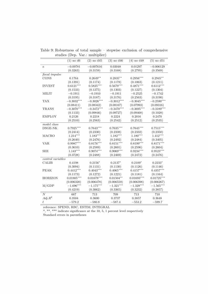
Table 9: Robustness of total sample – stepwise exclusion of comprehensivestudies (Dep. Var.: multiplier)

(1) no d6 (2) no d45 (3) no d46 (4) no d48 (5) no d51

κ −0.09781 −0.007616 0.03048 0.01297 −0.006129(0.3263) (0.3159) (0.3168) (0.2795) (0.3569)

fiscal impulseCONS 0.1764 0.2649∗∗ 0.2835∗∗ 0.2956∗∗∗ 0.2945∗∗

(0.1391) (0.1174) (0.1178) (0.1063) (0.1211)INVEST 0.6121∗∗∗ 0.5825∗∗∗ 0.5679∗∗∗ 0.4871∗∗∗ 0.6112∗∗∗

(0.1533) (0.1275) (0.1303) (0.1227) (0.1304)MILIT −0.1911 −0.1910 −0.1911 −0.2525 −0.1742

(0.3195) (0.3187) (0.3176) (0.2563) (0.3190)TAX −0.3032∗∗∗ −0.3026∗∗∗ −0.3012∗∗∗ −0.3045∗∗∗ −0.2590∗∗∗

(0.08411) (0.08342) (0.08167) (0.07993) (0.09316)TRANS −0.3070∗∗∗ −0.3472∗∗∗ −0.3470∗∗∗ −0.3695∗∗∗ −0.3189∗∗∗

(0.1133) (0.09846) (0.09727) (0.09468) (0.1028)EMPLOY 0.2126 0.2218 0.2224 0.2016 0.2470

(0.2510) (0.2563) (0.2542) (0.2512) (0.2535)model classDSGE-NK 0.7925∗∗∗ 0.7643∗∗∗ 0.7635∗∗∗ 0.7645∗∗∗ 0.7515∗∗∗

(0.2414) (0.2330) (0.2338) (0.2332) (0.2350)MACRO 1.214∗∗∗ 1.183∗∗∗ 1.182∗∗∗ 1.180∗∗∗ 1.412∗∗∗

(0.2640) (0.2476) (0.2492) (0.2484) (0.3405)VAR 0.9987∗∗∗ 0.8176∗∗∗ 0.8151∗∗∗ 0.8199∗∗∗ 0.8171∗∗∗

(0.3610) (0.2589) (0.2601) (0.2596) (0.2604)SEE 1.143∗∗∗ 0.9074∗∗∗ 0.9069∗∗∗ 0.9234∗∗∗ 0.9523∗∗∗

(0.3728) (0.2488) (0.2469) (0.2472) (0.2476)control variablesCALIB 0.4198 0.2156∗ 0.2137∗ 0.2109∗ 0.2233∗

(0.3094) (0.1131) (0.1130) (0.1126) (0.1146)PEAK 0.4412∗∗∗ 0.4043∗∗∗ 0.4065∗∗∗ 0.4157∗∗∗ 0.4357∗∗∗

(0.1173) (0.1272) (0.1221) (0.1181) (0.1164)HORIZON 0.01805∗∗∗ 0.01678∗∗∗ 0.01504∗∗ 0.01693∗∗∗ 0.01725∗∗∗

(0.006320) (0.006478) (0.006559) (0.006398) (0.006267)M/GDP −1.696∗∗∗ −1.175∗∗∗ −1.321∗∗∗ −1.329∗∗∗ −1.565∗∗∗

(0.4219) (0.3062) (0.3365) (0.3232) (0.3857)N 667 713 709 713 710Adj.R2 0.3504 0.3600 0.3737 0.3857 0.3648` −579.2 −580.8 −587.4 −553.2 −599.7reference: SPEND, RBC, ESTIM, INTEGRAL*, **, *** indicate significance at the 10, 5, 1 percent level respectivelyStandard errors in parentheses

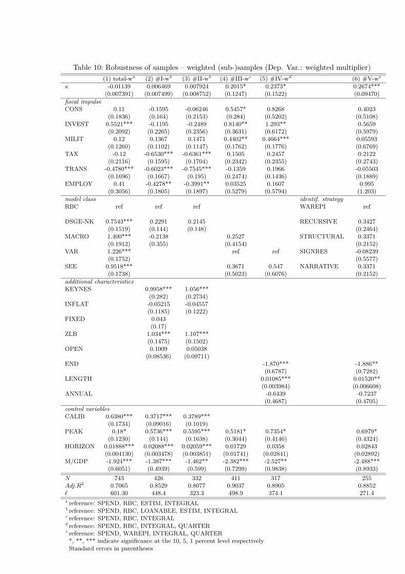
Table 10: Robustness of samples – weighted (sub-)samples (Dep. Var.: weighted multiplier)(1) total-wa (2) #I-wb (3) #II-wb (4) #III-wc (5) #IV-wd (6) #V-we

κ -0.01139 0.006469 0.007924 0.2015* 0.2373* 0.2674***(0.007391) (0.007499) (0.008752) (0.1247) (0.1522) (0.09470)

fiscal impulseCONS 0.11 -0.1595 -0.06246 0.5457* 0.8268 0.4023

(0.1836) (0.164) (0.2153) (0.284) (0.5202) (0.5108)INVEST 0.5521*** -0.1195 -0.2489 0.8140** 1.293** 0.5659

(0.2092) (0.2265) (0.2356) (0.3631) (0.6172) (0.5979)MILIT 0.12 0.1367 0.1471 0.4402** 0.4664*** 0.05593

(0.1260) (0.1102) (0.1147) (0.1762) (0.1776) (0.6769)TAX -0.12 -0.6530*** -0.6361*** 0.1505 0.2457 0.2122

(0.2116) (0.1595) (0.1704) (0.2342) (0.2355) (0.2743)TRANS -0.4780*** -0.6023*** -0.7545*** -0.1359 0.1966 -0.05503

(0.1696) (0.1667) (0.195) (0.2474) (0.1436) (0.1889)EMPLOY 0.41 -0.4278** -0.3991** 0.03525 0.1607 0.995

(0.3056) (0.1805) (0.1897) (0.5279) (0.5794) (1.203)model class identif. strategyRBC ref ref ref WAREPI ref

DSGE-NK 0.7543*** 0.2291 0.2145 RECURSIVE 0.3427(0.1519) (0.144) (0.148) (0.2464)

MACRO 1.400*** -0.2138 0.2527 STRUCTURAL 0.3371(0.1912) (0.355) (0.4154) (0.2152)

VAR 1.226*** ref ref SIGNRES -0.08239(0.1752) (0.5577)

SEE 0.9518*** 0.3671 0.547 NARRATIVE 0.3371(0.1738) (0.5023) (0.6076) (0.2152)

additional characteristicsKEYNES 0.9958*** 1.056***

(0.282) (0.2734)INFLAT -0.05215 -0.04557

(0.1185) (0.1222)FIXED 0.043

(0.17)ZLB 1.034*** 1.107***

(0.1475) (0.1502)OPEN 0.1009 0.05038

(0.08536) (0.09711)END -1.870*** -1.886**

(0.6787) (0.7282)LENGTH 0.01085*** 0.01520**

(0.003984) (0.006608)ANNUAL -0.6439 -0.7237

(0.4687) (0.4705)control variablesCALIB 0.6380*** 0.3717*** 0.3789***

(0.1734) (0.09016) (0.1019)PEAK 0.18* 0.5736*** 0.5595*** 0.5181* 0.7354* 0.6979*

(0.1230) (0.144) (0.1638) (0.3044) (0.4146) (0.4324)HORIZON 0.01888*** 0.02088*** 0.02059*** 0.01729 0.0358 0.02843

(0.004130) (0.003478) (0.003851) (0.01741) (0.02841) (0.02892)M/GDP -1.924*** -1.387*** -1.462** -2.382*** -2.527** -2.488***

(0.6051) (0.4939) (0.599) (0.7299) (0.9838) (0.8933)N 743 426 332 411 317 255Adj.R2 0.7065 0.8529 0.8077 0.9037 0.8905 0.8852` 601.30 448.4 323.3 498.9 374.1 271.4a reference: SPEND, RBC, ESTIM, INTEGRALb reference: SPEND, RBC, LOANABLE, ESTIM, INTEGRALc reference: SPEND, RBC, INTEGRALd reference: SPEND, RBC, INTEGRAL, QUARTERe reference: SPEND, WAREPI, INTEGRAL, QUARTER*, **, *** indicate significance at the 10, 5, 1 percent level respectivelyStandard errors in parentheses

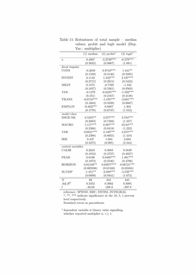
Table 11: Robustness of total sample – medianvalues; probit and logit model (Dep.Var.: multiplier)

(1) median (2) probita (3) logita

κ 0.4007 -3.2739*** -6.579***(0.3032) (0.9867) (1.881)

fiscal impulseCONS -0.2059 0.8743*** 1.441**

(0.1539) (0.3146) (0.5985)INVEST 0.1142 1.342*** 2.197***

(0.2715) (0.2915) (0.5422)MILIT 0.1575 -0.7769 -1.342

(0.1857) (0.5361) (0.9503)TAX -0.1279 -0.8235*** -1.502***

(0.161) (0.2167) (0.4138)TRANS -0.6710*** -1.476*** -2.601***

(0.1604) (0.3339) (0.6667)EMPLOY -0.3827** 0.8987 1.303

(0.1778) (0.6747) (1.552)model classDSGE-NK 0.5355** 2.077*** 3.784***

(0.2083) (0.7488) (1.347)MACRO 1.117*** 8.887*** 23.84***

(0.2386) (0.8418) (1.223)VAR 0.6621*** 2.130*** 3.874***

(0.2398) (0.8055) (1.419)SEE 0.437 1.084 2.094

(0.3275) (0.995) (2.344)control variablesCALIB 0.2623 0.3683 0.5849

(0.1852) (0.2727) (0.4927)PEAK 0.0196 0.8480*** 1.481***

(0.1072) (0.2546) (0.4706)HORIZON 0.01549** 0.03977*** 0.06721***

(0.005936) (0.01348) (0.02494)M/GDP -1.451** -2.698*** -4.556***

(0.6899) (0.9441) (1.674)N 89 641 641Adj.R2 0.3352 0.3062 0.3085` -49.69 -298.9 -297.9reference: SPEND, RBC, ESTIM, INTEGRAL*, **, *** indicate significance at the 10, 5, 1 percentlevel respectivelyStandard errors in parentheses

a dependent variable is binary value signalling,whether reported multiplier is <≥ 1.

Publisher: Hans-Böckler-Stiftung, Hans-Böckler-Str. 39, 40476 Düsseldorf, Germany Phone: +49-211-7778-331, IMK@boeckler.de, http://www.imk-boeckler.de

IMK Working Paper is an online publication series available at: http://www.boeckler.de/imk_5016.htm

ISSN: 1861-2199 The views expressed in this paper do not necessarily reflect those of the IMK or the Hans-Böckler-Foundation. All rights reserved. Reproduction for educational and non-commercial purposes is permitted provided that the source is acknowledged.