NASA Contractor Report 198488AIAA-96-1780

Refraction and Shielding of Noisein Non-Axisymmetric Jets

Abbas KhavaranNYMA, Inc.

Brook Park, Ohio

May 1996

Prepared forLewis Research Center

Under Contract NAS3-27186

National Aeronautics and

Space Administration

https://ntrs.nasa.gov/search.jsp?R=19960023935 2018-05-26T11:06:19+00:00Z

Refraction and Shielding of Noisein Non-Axisymmetric Jets

Abbas Khavaran *

NYMA, Inc., Lewis Research Group, Cleveland, OH 44135

Abstract

This paper examines the shielding effect of the

mean flow and refraction of sound in non-axisymmetric

jets. A general three-dimensional ray-acoustic ap-proach is applied. The methodology is independent

of the" exit geometry and may account for jet spread-

ing and transverse as well as streamwise flow gradients.

We assume that noise is dominated by small-scale tur-

bulence. The source correlation terms, as described

by the acoustic analogy approach, are simplified and

a model is proposed that relates the source strengthto 7/2 power of turbulence kinetic energy. Local char-

acteristics of the source such as its strength, time- or

length-scale, convection velocity and characteristic fre-

quency are inferred from the mean flow considerations.

Compressible Navier Stokes equations are solved with

a k-e turbulence model. Numerical predictions are pre-

sented for a Mach 1.5, aspect ratio 2:1 elliptic jet. Thepredicted sound pressure level directivity demonstrates

favorable agreement with reported data, indicating arelative quiet zone on the side of the major axis of the

elliptic jet.

a,baoo

a(x)c(x)Degk

M

Pi

$

T

U¢

u_Vi

6_

0

Nomenclature

length of semi major and minor axesfreestream sound speed

local sound speed

normalized sound speed

area equivalent jet diameter

turbulent kinetic energy = vivi/2Mach vector

component of phase normal p

arc length

turbulence intensity =v-"_/3

source convection velocity

jet exit velocity

fluctuating velocity component

dissipation rate of kinetic energy

= _,(OvilOZ_ )(Ovi IOX_ )polar observer anglemomentum thickness

elliptic coordinates

* Senior Research Engineer, Member AIAA.

PT

¢_

SubscriptsO

OO

density

time-delay of correlation

azimuthal observer angle

observer and source frequencies

source locationfar field

1. Introduction

The aim of the present study is to determine the

far-field directivity of sound due to a jet issued from a

non-axisymmetric exit plane. The theoretical argument

is a derivative of Lighthill's Acoustic Analogy, withmodifications to account for the three-dimensional re-

fraction effects. It is generally accepted that, in theory,

direct numerical simulation (DNS) based on the full,

compressible Navier-Stokes equations govern both the

generation and propagation of sound. Current efforts

in computational aeroacoustics 1 (CAA) are directed to-wards resolving various computational issues, such as

grid resolution (for frequencies of interest), computa-tional domain, boundary conditions, finite difference

scheme and so on. The presence of shock expansion

fans, under imperfectly expanded conditions, will re-quire additional attention in order to predict the shock-associated noise.

Apart from DNS, other computational models will

require some sort of turbulence modeling to predict

the mixing noise of a typical shock-free jet. For ex-anaple, Mankbadi et. al _,3 have opted for an extension

of the large-eddy simulation approach (LES). This ap-

proach, models the fine-scale turbulence and calculates

the large-scale components from the filtered Navier-

Stokes equations. The calculated sound field is thusassociated with the large-scale turbulence. Further

simplifications were proposed 4,5 by neglecting viscos-

ity and nonlinear effects utilizing linearized Euler equa-

tions (LEE). This last approach is less computer inten-

sive and has been suggested as an alternative to (LES)

for three-dimensional geometries. Sample predictions

with LES and LEE are presented in the references cited

above. The results are encouraging and succeed in cap-

turing the near-field directivity of jet noise at Strouhal

numbersofinterest.

Lighthill'sformulations,on theotherhand,sug-gestsa sourcecorrelationtermbasedprimarilyontheunsteadyvelocityfluctuations.Complicationsassoci-atedwithnumericalcalculationof the Lighthill's source

term have resulted in various modeling efforts. These

efforts have produced alternatives to Lighthill's source

term, such as those derived from a mean flow so-

lution and with an appropriate turbulence modeling.

Meanwhile, the flow-acoustic interaction is explicitlyaccounted for as an additional superimposing term.

We start with a brief review of the source modeling

as derived from a compressible Navier-Stokes solution

with a k-e turbulence model (e.g., Ref. 6). Our focus,

however, is the assessment of the mean flow effects on

directivity of jet noise.

Two models are proposed for acoustic predictions.

These models differ in the application of flow-acousticinteraction. The first model incorporates Balsa's 7 so-

lution. Balsa examines the high frequency solution to

Lilley's equation in a cylindrical coordinate system. Heobtains directivity factors for each of the quadrupoles

contained within a turbulent eddy volume element. To

extend Balsa's solution to non-axisymmetric jets, we

apply a quasi-3D approach. This is done by integrating

Balsa's solution azimuthally, i.e., treating each stream-

wise jet slab as a representative of the entire jet volume.

The predicted sound field, though void of any azimuthal

directivity, may be argued to account for 3D distribu-

tion in source strength as well as the surrounding meanflOW.

In the second model, a full 3D ray-acoustic ap-

proach is applied. A system of six propagation equa-

tions is solved numerically in a rectangular coordinate

system. We map the CFD solution to a uniform grid,

i.e., a grid independent of the streamwise direction,

and apply a throe-dimensional spline interpolation on

flow parameters of interest. Mean flow gradients arecomputed readily from the ensuing spline coefficients

as the numerical solution of refraction equations pro-

coeds along rays of geometric acoustics. Although a

ray-acoustic solution succeeds in capturing the far-fieldazimuthal variation in sound, the intensive numerical

computations suggest that the methodology should beconsidered only when the non-axisymmetric exit geom-

etry may result in a relatively significant azimuthal di-

rectivity.

The source characteristic is described similarly in

both approaches. This includes the simplification offourth-order space-time correlations 6 and separation of

space and time factors. A new function is proposed for

the time-factor of the correlation. This function, re-

placing the Gaussian distribution employed in the ear-lier models 11, helps improve the predicted spectra.

As an example, a shock-free Mach 1.5 elliptic jet

with aspect ratio of 2:1 is selected. Aerodynamic pre-

dictions are compared with data as well as predictions

for a base convergent-divergent round nozzle, operatingat similar conditions. The acoustic predictions include

sound pressure level directivity (SPL), as well as 1/3-

octave band spectra.

2. Method of Solution

It is generally recognized that at subsonic andlower supersonic speeds, small scale turbulence is the

primary acoustic source. Each finite volume of tur-

bulence, may be described as a multipole source thatconvects downstream and emits sound that is refracted

by mean flow gradients. As jets becomes highly su-

personic, large-scale structures or instability waves ofthe flow s become increasingly more active. In the

present study, we assume that fine-scale turbulence is

the source of jet noise. With a compact eddy approx-

imation, the solution is usually expressed as a Fourier

transform of space-time correlation function, integrated

over the entire jet volume. Availability of unsteady flowsolutions should, in principle, make it possible to com-

pute correlation functions of various order and orien-

tation. Today's computational capabilities, perhaps,

should encourage this effort, at least, for a selectednumber of source volume elements within the jet. Theimmediate benefit would include assessment of a num-

ber of simplifying assumptions that have traditionally

been employed for source modeling. For the present

work, however, we follow an approach based on separa-

bility of space-time correlation and rather focus on re-fraction and shielding of non-axisymmetric geometries.

2.1 Source and Spectra

As described previously, any attempt to integrate

the source correlation function over the jet volume re-

quires modeling of these functions. Reference 6 outlinesa procedure used in the present study and we briefly

discuss some of the more important steps. Roughly

speaking, various regions of turbulence of size _, com-

monly referred to as an eddy volume element, radi-ate sound to far-field that may be summed up for all

regions of the jet if the correlation volume elementsradiate independently. In addition, acoustical com-

pactness which allows for the use of elementary so-

lutions like simple sources to model complex sourcesof sound such as quadrupoles requires that wi/a_ be

small. This condition requires that the r.m.s, velocityfluctuation be small relative to ambient sound speed 9

, i.e., < v 2 >1/2/aoo << 1, which makes the turbulence

length-scalesmallrelativeto theacousticwavelength.It shouldbenotedthat thecompactnessconditionisnotthatrestrictiveandmayholdtrueevenatmoderateMachnumbers.Assumingthat noiseis dominatedbyfine-scaleturbulence,contributionsfromtheself-noiseterm,in absenceofrefractionandconvection,isshownto bedueto afourth-orderspace-timecorrelationfunc-

• . t_)l.tion v, viv _ t As is usually done, the above term is

expressed as a linear combination of second-order cor-

relations viva. This is followed by the space-time sepa-

ration given as vivj = R_/(0g(r), where (and r are theseparation vector and time-delay respectively. For ho-

mogeneous isotropic turbulence, Batchelor 1° suggests a

space function of the form

÷ (:IDetails of f(() are provided in Ref. 10 and are not re-peated here. A Gaussian function is normally selected

for the time-factor part as g(r) = ezp(-r2/r_), with

7-orepresenting the characteristic time-delay of the cor-

relation. It was shown (Ref. 6) that Vo may be derived

from the ratio of kinetic energy of turbulence k and itsdissipation rate e as 1/ro ,., e/k. Noise spectra is calcu-lated from the Fourier transform of the autocorrelation

function

//I(a) = g2(v)einrdr (2)

which results in I(12) _= ro_/_r/ze 8 . In generalfunction g(v) may be written to include other powers

of r. For example function

g(T) = (3)

with positive constants cl, c2 and c3 transforms the

above integral into a series of modified Bessel functionsK and with added empiricism as a result of the new

constants. With c3 = 0 and g(T) = e -c'(_l_*)2-c_l_/T°lwe have

I(O) = ,r--_°_vr_Re{eT'ercf(T)} (4a)zVcl

where

T - c2 - i(nro/2) (4b)

and ercf(T) denotes a complementary error function.

Constant c2 provides additional flexibility to shape the

spectra at higher frequencies. With c2 = 0, the solution

reduces to that given in Ref. 11. All acoustic predic-

tions presented here are based on equation (4a) withci = 2.0 and c2 = 1.0e-5.

Noise spectra due to a unit volume of turbulence,

and arising from the source correlation term VlVlV_V{

may be written as

3 2 ½(_ro)4 I T 2

(5)A Doppler factor relates source frequency D to the ob-server frequency w. Contributions from other source

correlation components Iijkt are expressed similarly 6.

2.2 Flow-Acoustic Interaction

It is known that the operator part of the Lilley's

equation accounts for refraction as well as convection.

A close-form solution to this equation was given by

Balsa 7 in the high frequency limit and in a cylindricalcoordinate system. Although Balsa's directivity factors

are limited to axisymmetricjets, the solution may be in-

tegrated azimuthally for various streamwise jet slices to

predict the SPL directivity for non-axisymmetric flows.

This type of prediction, referred to as a quasi-3D solu-

tion, though void of any azimuthal variation in sound, isvery robust and should be considered a first approxima-

tion to noise prediction for arbitrary geometries when

far-field azimuthal directivity is relatively small.

The general directivity of sound for jets of arbi-

trary geometry may be assessed using ray-acoustics in

a high frequency limit. In a high frequency approxi-mation, it is normally assumed that the acoustic wave

length is shorter than the characteristic length of the

mean flow. For high speed jets, this approximation can

be used effectively to predict the more energetic part of

the sound spectra and for Helmholtz numbers (fD/aoo)

as small as one (see Tester and Morfey12). When a

parallel flow approximation is invoked, refraction of jetnoise through a sheared mean flow of arbitrary geom-

etry may be formulated as a two-dimensional geomet-

ric acoustic problem 13. It is argued 14 that for high

speed flows, jet spreading may play a significant role in

defining the size of cone of silence which is formed in

the neighborhood of the downstream jet axis. In suchcases, flow spreading may be accounted for by formu-

lating a three-dimensional ray-acoustic problem. Thus,as acoustic energy, released from each finite volume of

turbulence propagates out of the shear-layer, its spread-

ing is inferred from the area of a ray-tube surrounding

that ray.

For an inviscid flow governed by linearized gas dy-

namic equations, the coordinate X of the emitted sound

at any point s along the ray is determined from a set

of six equations 14'15

dX___f=ds _JPJ + Mi/C i,j = 1,2,3

dpids

and

_ 1 07)k 0 .Mj. 1g (c (6a)

Tq = 6ij - MiMe

u(x) c(x)- a(x) (6b)M(X)-- a(X)' aoo

Vector p is normal to the phase front and Mi denotes

the component of the Mach vector M. Equations (6)

are solved numerically subject to initial conditions as-sociated with the source location and direction of emis-

sion. Let unit vector X = (cos gt, sin # cos 6, sin I_ sin 6)denote the direction of emission at the source, and sub-

scripts o and oo refer to source and observer locations

respectively, then

X = Xo at s = 0

1 M

Po = A:X + (A_:. M - _)_-, (7a)

_!

,_=[32+(:K.M) 2] _/C, 32= 1-1M[S. (7b)

As rays emerge from the shear layer, they become

straight and the ray speed A approaches one. For every

set of radiation angles (/_, 6) a pair of angles (/900, ¢co)

may be calculated from equations (6). Variation ofthe ray-tube area is then expressed as the Jacobian of

the transformation, i.e., I (9(000, ¢oo)/O(p, 8) I. It isshown 14,16 that the far-field mean square pressure di-

rectivity for a convecting quadrupole source of strength

Qij(fl) becomes

2 3

oc (pooaoo)_4(Qijpipj _2( ao Ao)×

(l-O* _ _=_1aoo.-P__o) t* -- a_ " Poo) = . sinp 1

¢1- po)s I I)(8)

where Ue is the source convection velocity and w is the

observer frequency related to source frequency f_ as

w = f_/(1 - U_..._¢.po). (9)_2oo

For an isotropic quadrupole source, Qijpipj = Qo Ip I_.If source spectral power density Q_ is replaced with

Inn/ft 4 from (5), the directivity pattern is found as

2 2

p2 o¢ aoo _ p_ k_ gtro 4R eT ercf T a° Aa oQ. ) d

(1- _Y-_""Po)2(1- u--_' Poo)u. sin. 1

× (1-=---_:Po_ (s/-_l_l)"

(10)

Roughly speaking, when the difference between Uo and

U¢ is small, and assuming that Uoo is negligible, thedirectivity pattern scales as (1 - _ • po) -3 outside the

zone of silence. Near and within the boundary of zone

of silence, the factor ('_.z!__Wl 0(0oo, ¢oo)/(9(/_, 6) 1hi-\ sin 0e, o 111

ters the above directivity and results in concentration

of noise near the boundary of zone of silence, i.e., a

sharp peak followed by a rapid decay into the zone ofsilence.

2.3 Aerodynamic Predictions

Flow predictions were made with the NPARCNavier-Stokes code and with a recently installed 17 low

Reynolds number k-e model of Chien is. The conical

and elliptic jets considered had an exit area of 1.571in 2 each, with aspect ratio of AR=2:I for the elliptic

jet. Both nozzles are operated at the design pressure

ratio of 3.67 and 564 ° R total temperature to give exit

Mach number of 1.5. Some aerodynamic and acousticdata 19 were available for validation. Because of symme-

try, only one quarter of the elliptic jet is modeled. The

major and minor axes are planes of symmetry modeled

with NPARC's slip wall boundary conditions. A grid

having 121 ×91 points in axial and radial directions and

25 points in circumferential direction was selected. The

domain of the grid includes 10 diameters into the nozzle

and up to 70 diameters downstream of the exit plane.

For convenience , elliptic coordinates _1 and _ areintroduced

y={xcos{2, z=(_l/p)sin_2, x=;c, (11)

where z denotes the streamwise direction. The above

coordinates maintain a constant aspect ratio ofp = a/b,

with an area element dA = (_1/p)d_ld_2 (see figure la).Within one quarter of the elliptic jet, the azimuthal an-

gle ¢, measured from the major axis, is equally divided

over 25 grid points and relates to elliptic angle _2 as

tan_2 = ptan _b. Two-dimensional views of the elliptic

grid for major axis plane zy and spanwise plane yz are

shown in figures lb and lc.

The centerline velocity decay for both 2D and3D flow predictions are sensitive to the selection of

the spanwise boundary conditions. With a free-type

boundary condition, the predicted centerline velocity

decay (figure 2) shows a supersonic core length of 11.9D

and l l.3Deq for round and elliptic jets compared to

14.2D and ll.2Deq reported experimentally 19. Al-

though a slip-type boundary condition will improve the

2D predictions (see Ref. 11), in the interest of 3Dacoustic predictions, however, boundary conditions fa-

vorable to elliptic jet are selected for mean flow com-

putations.

Velocityprofilesalongthemajorandminoraxesof the elliptic jet are shown in figures 3a and 3b respec-tively. Comparison with data of Seiner 19 demonstrates

good agreement along the minor axis plane. The major

axis predictions, on the other hand, appear to under-

estimate the spreading rate. Similar conclusions weredrawn from the axial distribution of momentum thick-

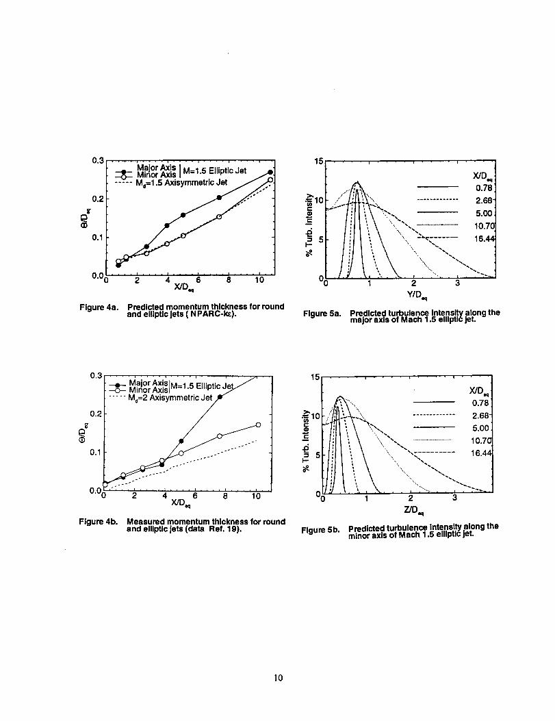
ness defined for compressible flows

fo ° pU UO = (p-_c/(1 - _-_z)dr, (12)

where subscript cl denotes the centerline values. The

predicted momentum thickness (figure 4a) shows little

difference along the major and minor axes near the exit.

A more pronounced difference is observed downstream

where thickness along the major axis shows a slightlyfaster growth rate. The round nozzle momentum thick-

ness in figure 4a is in agreement with the elliptic jet's

minor axis. Data of figure 4b indicates that momen-

tum thickness is nearly equal along both axes over the

length of the potential core and starts to grow at afaster rate along the major axis near the end of thecore. Notice that the round nozzle momentum thick-

ness, shown here for a design Mach number of 2.0, is in

agreement with the general behavior along the minor

axis as was concluded from predictions of figure 4a.

Predicted turbulence intensity profiles along major

and minor axes of the elliptic jet are shown in figures5a and 5b. Here the percent turbulence is defined as

100 x (vivi/3)l/2/Uj. Both figures indicate a maximum

level in the neighborhood of the jet lip-line and an exit

value of 11.3%, that will gradually increase to 12.5%

at about 5Deq and decays farther downstream. The

centerline value is zero within the core to about 6Deqand will rise to 3.4% at 7.3D_q and 8.7% at 10.7Deq.Although the existing modifications 17 in NPARC allow

for turbulence kinetic energy input as an inflow bound-

ary condition, the predictions within the core remain

insensitive to the specified inflow values. Experiments

should be performed to verify turbulence predictions.

2.4 Acoustic Predictions

A quasi-3D predictionmodel may be employed to

predictthe noiseof3D jetswhen the azimuthal direc-

tivityisoflesssignificance.This isdone by integrating

Balsa'ssolutionazimuthally,i.e.,treatingeach stream-

wise jet slab as a representativeofthe entirejet.The

approach isnumerically robust and should be consid-

ered as a viablesolutionwhen azimuthal directivityis

not a design criteria.Geometries such as round lobed-

mixer nozzles may not result in a significant azimuthaldirectivity in the far-field. This is more so with increas-

ing the number of lobes.

Sample prediction for Mach 1.5 elliptic jet us-ing a quasi-3D approach will be discussed shortly. A

full 3D ray-acoustic solution, on the other hand, is

obtained according to equation (10) and in conjunc-

tion with equations (6) and (7). Here, as in the 2Dcase, source strength k 7/2 and characteristic time-scale

7"o are derived from CFD- ke solutions according to1/7"o = a(e/k). Empirically constant a is included

in constant cl. Source convection velocity Uc is ex-

pressed as weighted average of exit and local velocities

Ue = 0.SUo + 0.3U]. For an observer frequency to, the corresponding source frequency f2 is calculated

from equation (9), where Po denotes the normal to the

phase front at the source. At selected observer coordi-

nates (R, 0oo, ¢_), the source radiation angles (p, 6)

and the corresponding phase normal Po are found by

solving (6) and (7) numerically as a boundary-value

problem. Once the missing initial values are found,

they may be used as a first guess for the neighboringsource volume element AV and the process continues.

In order to integrate the propagation equations, a

B-spline interpolation of the CFD solutions is carriedout in three dimensions

N{2 N¢1 N=

/=1 m=l n=l

Bt,k,_,,,_ (_2) = f(z, _1, (_). (13)

Tensor coefficients Cnmt may be found for each flow pa-

rameter of interest by solving (13) as a system of simul-

taneous equations applied to data points (z, _1, _2, f)-

Here k,, k¢_ and k_2 are the orders of spline , t,, t_

and t_ are the corresponding knot sequence in z, (1

and (z directions respectively 23, and Bn,_,, denotes then-th B-spline of order k with respect to knot sequence

t. It should be noted that the above process assumes

a uniform grid, i.e., one independent of the streamwise

direction. To this end, a postprocessing of the CFDsolution may be necessary. This is usually done by se-

lecting a common spanwise grid structure, say one de-

fined at X/Deq = 10.0, and consequently mapping the

flow field to this grid at each streamwise location using

a two-dimensional B-spline interpolation. Once spline

coefficients Cnmt in equation (13) are determined, the

directional derivatives become readily available at anypoint within the jet.

It is known that refraction results in a zone of si-

lence for the high frequency noise. The zone of silence,

denoted as O*(Xo), and measured from the jet axis, is

defined as the smallest polar angle that may receive

acoustic signal from a source. This angle is found ateach source location Xo by solving equations (6) sub-

jet to initial conditions (/_, 6) = (0, 0). Obviously, for

off-axissources,acompleterefractionmaybeachieved

with a small value of cone angle/a if _ is such that soundis directed towards the centerline. This may explain the

observed smooth transition of SPL directivity into the

zone of silence. However, the peak directivity level for

a selected source is in the very neighborhood of 8*.

Shown in figure 6 is the boundary of zone of silencefor sources located on the major axis plane, x-y, of the

elliptic jet. The source axial location is indicated as the

parameter Xo/Deq. It is clearly seen that for the most

part, more energetic segments of the jet, i.e. sourcesnear the lip-line Yo/a = 1.0, radiate primarily in direc-tion of 0* = 50% This is consistent with the reported

directivity for the high Strouhal number noise for Mach

1.5 elliptic jet. Sensitivity of the zone of silence with

respect to azimuthal source location is shown in figure7. Generally speaking, the flow asymmetry will resultin an increase in the size of cone of silence as the source

moves azimuthally closer the minor axis.

Sound pressure level directivity for elliptic jet as

well as Mach 1.5 conical jet are shown in figure 8. Pre-dictions are on a 12 foot sideline. Here, the elliptic

jet is treated with the quasi-3D approach. This type

of prediction, as indicated earlier, does not produce anazimuthal directivity. Also shown in this figure is the

measured SPL directivity 19. Noise measurements of

non-axisymmetric flows, normally show lower noise on

the deep side of a jet, such as the major axis of the

elliptic jet. In addition, asymmetric jets usually gener-ate less noise compared to conical jets operating under

similar conditions. This may be due a combination of

factors such as turbulence level, enhanced mixing, and

decay in supersonic core length. No data was availablefor the conical nozzle at this point, however, based on

measurements reported at higher temperatures 24, it is

anticipated that the conical nozzle is at least as noisy asthe minor axis side of the elliptic jet. Predictions of fig-

ure 8 indicate a reasonably good agreement with data

in the peak noise level, though the size of the zone of si-lence seems somewhat exaggerated. Predicted spectra

for the two jets are shown in figures 9 and 10.

We apply a three-dimensional geometric acoustic

(3DGA) approach to assess the general directivity ofsound for the elliptic jet. A matrix of five polar angles

0oo = 50 ° to 110 °, in increments of 15 °, and four az-

imuthal angles ¢oo = 0 ° to 90 °, increments of 30 ° isselected.

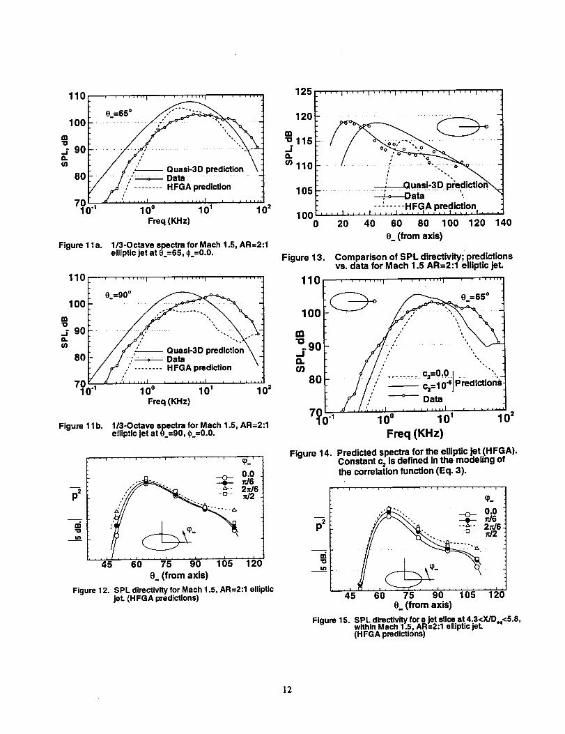
Shown in figures lla and llb are the HFGA spec-

tral predictions along the major axis side of the elliptic

jet. Spectral measurements, converted to 1/3-octaveband, as well as the quasi-3D predictions are shown in

these figures. Data shows some shift in the spectral

peak to higher frequencies with increasing polar angle

000. The prediction methods do not exhibit a similarshift as data. It is conjectured that this may be asso-

ciated with simplistic replacement of the fourth-order

space-time correlation functions.

Azimuthal directivity (figure 12), for the most

part, shows 2 dB lower noise along the major axis side,

in good agreement with data of figure 8. Due to theimmense numerical calculations associated with ray-

acoustic predictions, the volume integration was lim-

ited to the more energetic elements within the jet. This

might reflect as several dB difference in the noise level

as seen in figure 13. In addition, predicted zone ofsilence appears much larger than measurements (fig-

ure 13). Arguably, this may relate to the absenceof a frequency-dependent factor in the first term of

the expansion series is selected for the GA predictions.

The directivity factors suggetsted by Balsa, though ob-tained in a high frequency limit, contain a wave number

factor. It is plausible that addition of the second term

in the expansion series could improve the ray-acoustic

predictions, in particular near the jet axis where low

frequency noise dominates. An accurate prediction of

the mean flow profiles and jet spreading may also have

a significant bearing on refraction angles. For example,

it was shown (Ref. 11 ) that an ambient Maeh numberof Moo = 0.1, will reduce the size of the zone of silence

by more that 8 degrees.

The significance of constant c2, as used in the the

present model for the time-delay function (see Eq. 3) is

shown in figure 14. It is seen that the predicted spectrashow improvements relative to case when c2 = 0.0.

Figure 15 demonstrates the spherical directivity

for a typical jet segment at 4.3 < X/Deq < 5.8. This

figure suggests that the basic azimuthal pattern of jetnoise may be captured readily by selection of appropri-

ate source elements within acoustically active regions

of the flow and without a need for complete volume

integration.

3. Concluding Remarks

We presented a methodology for prediction of jet

mixing noise due to noncircular jets. A shock-free el-liptic jet with an aspect ratio of AR=2:I was consid-

ered. Predictions assume that noise is generated bysmall scales of motion and is dominated by the high

end of the spectra.

Two prediction models were proposed. A quasi-3D

methodology, based on Balsa's solution, should be con-sidered when the azimuthal directivity is of less signifi-

cance. This approach accounts for asymmetry in sourcedistribution as well as the surrounding mean flow, how-

ever, the predicted directivity is axisymmetric. A full

3D ray-acoustic solution ,derived from the first term in

theexpansionseries,generatesanazimuthaldirectiv-ity compatiblewith datawhilethepredictedzoneofsilenceremainslargerthanmeasurements.

Contributionsfromlarge-scalecoherentstructuresmaybeaccountedforviaalinearinviscidstabilityanal-ysis.Stabilitytypeanalysisis highlygeometrydepen-dentandhasbeenfully exploredin Ref. 22for anellipticgeometryassuminga simplerepresentationofthemeanvelocityprofiles.

Asdiscussed,arevisitoftheturbulencecorrelationfunctionforthepurposeofsourcemodelingandvalida-tion is appropriateat this point.Despitethisneededimprovement,ray-acousticapproachaspresentedhere,shedslightontheimportanceofthemeanflowinterac-tionandtheroleit playsin shapingthedirectivityofjet noise.

4. AcknowledgementsThisworkwassupportedbyNASALewisResearch

ContractNAS3-27186.ThetechnicalmonitorwasE.A. Krejsa.Theauthorisgratefulto Dr. 3.M.Seinerfrom NASALangleyfor supplyingthe experimentaldata.

References

1Tam,C. K. W. andBurton,D. E., "SoundGener-atedby InstabilityWavesof SupersonicFlows.Part2. AxisymmetricJets,"J. Fluid Mech., 138, 1984, pp.273-295.

2Mankbadi, R. R., Hayder, M. E. and Povinelli, L.

A., "Structure of Supersonic Jet Flow and its Radiated

Sound," AIAA Journal, 32 , 1994, pp. 897-906.

3Mankbadi, R. R., Shih, S. H., Hixon, R., and

Povinelli, L. A., "Direct Computation of Acoustic andFlow Field of a Supersonic :let Using Large-Eddy Sim-

ulation," AIAA Paper 95-0680, 1995.

4Mankbadi, R. R., Hixon, R., Shih, S. H., and

Povinelli, L. A., "On the Use of Linearized Euler Equa-tions in the Prediction of Jet Noise," AIAA Paper 95-

0505, 1995.

SHixon, R., Shih, S. H., and Mankbadi, R. R., "Ef-

fect of Input Disturbance on Linearized Euler EquationPrediction of Jet Noise," AIAA Paper 96-0752, 1996.

6Khavaran, A., Krejsa, E. A., and Kim, C. M., "Com-

putation of Supersonic Jet Mixing Noise for an Axisym-metric Convergent-Divergent Nozzle," AIAA J. Air-

craft, 31, 1994, pp. 603-609.

7Balsa, T. F., "The Far Field of High Frequency Con-

vected Singularities in Sheared Flows, with an Applica-tion to Jet Noise Prediction," J. Fluid Mech., 74, 1976,

pp. 193-208.STam, C. K. W., "Aerodynamics of Flight Vehicles:

Theory and Practice," NASA Ref. Pub. 1258, Vol. 1,

1991, pp. 311-390.

9Lighthill, M. 3., "Jet Noise. The Wright Brothers'

Lecture," AIAA Journal., 1, 1963, pp. 1507-1517.l°Batchelor, G. K. The theory of Homogeneous Tur-

bulence, Cambridge Univ. Press, 1953.

11Khavaran, A., and Georgiadis, N. J., "Aeroacous-

tics of Supersonic Elliptic Jets," AIAA Paper 96-0641,1996.

12Tester, B. J. and Morfey, C. L., "Developments in

Jet Noise Modeling- Theoretical Predictions and Com-parisons with Measured Data," J. Sound Vib., 46(1),

1976, pp. 79-103.

laGoldstein, M. E., "High Frequency Sound Emission

from Moving Point Multipole Sources Embedded in Ar-

bitrary Transversely Sheared Mean Flows," J. Sound

Vib.,80(4), 1982, pp. 499-522.14Khavaran, A., and Krejsa, E. A., "Refraction of

High Frequency Jet Noise in an Arbitrary Jet Flow,"

AIAA Paper 94-0139, 1994.lSDurbin, P. A., "High Frequency Green Function for

Aerodynamic Noise in Moving Media, part I: General

Theory," J. Sound Vib., 91(4), 1983, pp. 519-525.

16Durbin, P. A., "High Frequency Green Function for

Aerodynamic Noise in Moving Media, part II: Noisefrom a Spreading Jet," J. Sound Vib., 91(4), 1983, pp.527-538.

17Georgiadis, N. J., Chitsomboon, T., and Zhu, 3."Modification of the Two-Equation Turbulence Model

in NPARC to a Chien Low Reynolds Number k-e For-

mulation," NASA TM-106710, 1994.

lSChien, K. Y., "Prediction of Channel and Boundary

Layer Flows with a Low Reynolds-Number Turbulence

Model," AIAA Journal, 20(1), 1982, pp. 33-38.

19Seiner, J.M., "Fluid dynamics and Noise Emission

Associated with Supersonic Jets," Studies in Turbu-

lence, edited by T.B.Getski, S. Sarkar and G. Speziale,

Springer-Verlag, New York, 1992, pp. 297-323.2°Ho, C. M. and Gutmark, E., "Vortex Induction and

Mass Entrainment in a Small Aspect Ratio Elliptic

Jet," J. Fluid Mech., 179, 1987, pp. 383-405.

21Bridges, J.E. and Hussain, A.K.M.F., "Roles of Ini-tial Condition and Vortex Pairing," J. Sound Vib., 117,

part 2., 1987, pp. 289-311.22Morris, P. J., and Bhat, T. R. S., "The Predic-

tion of Noise Radiation from Supersonic Elliptic Jets,"

AGARD 78th Specialist Meeting on Combat Aircraft

Noise, Bonn, Germany, Oct. 1991.23de Boor, C., A Practical Guide to Splines, Springer-

Verlag, New York, 1978

24Seiner, J. M., and Ponton, M. K., "SupersonicAcoustic Source Mechanisms for Free Jets of Vari-

ous Geometries," AGARD 78th Specialist Meeting on

Combat Aircraft Noise, Bonn, Germany, Oct. 1991.

Z dA

Figure l a. Elliptic coordinates

[iiiilllllli uillJ liljllllJllllLI i i i-4---r"

,...-m"

-"r" f

0.9

0.8

5-0.7

0.6

0.5

.1 .... , .... , .... , .... , .... , .... ,.

1.0 .....,"""-

__,. ..... Elliptic(Data)

_'_ -- Elliptic(Chieflk-c)"_'., Round(Data)

0.4'.

0.30 5 10 15 20 25 30

X/Deq

Figure 2. Centerline velo.citydecay for the elliptic jetand the equivalent M=1.5 conical je[.

Figure lb. Grid in major axis plane,jet exit is at X=0.0.

X

Figure lc. Grid in a spanwise plane at YJD,q=5.4.

1.0

0.5

U/U i

DataChien-k_

1.0_

X/D_=0.088

Z/D,,q

1.0 1.5

0.5

O

%'.0' ' "0.s.......... ' 0._

0

k_, X/D,q=5.057

........ ._.°°O0_OQ°°?°°?,0 0.5 1.0 1.5 2.0 2.5

o:LX/D,q=1.265

0 0 0 0 0,0 0 0 O0

0. ' ' ' '0.5 .... 1.0' 11.5

1.0

%

0"_

........... _°00°_ J0.%,.00.5 1.0 1.5 2.0 2.s

Figure 3a. Velocity profile along the minor axis of the elliptic jet.

U/Uj0

1.0 _' o _ _'X%

0

0.5

X/D,,q=0.088

%'.0 0.s

o DataChien-k¢

o Y/D_

...... 151 '.0 1

I"0_ -_o o

0.5 _,o

\o

X/D'4--5"057 "",__ o o o o o

%'.d- b.'S _0 _o 2'.0 2:s

1.0_ c. o _o

0.5- 265 _ °X/D,q=1.

O O O, , J

0"_'.0 .... 0:5 ' " 110 1.5

1.0

°Oo0.5 _o

X/D_=10. o o o

Figure 3b. Velocity profile along the major axis of the elliptic jet.(NPR=3.67, T=104 ° F, AR=2:I, M =0.0)

.3 .... i .... i .... i .... _ .... i . .

Major Axis• M=I 5 Elliptic JetM,.orAxls] • " j'_:

0.2 ..'"'" :

006.... 2 .... _ .... _ .... _ .... 1oX/D,q

Figure 4a. Predicted momentum thickness for roundand ellipUc Jets ( N PARC-k_).

15 i . ! .... i ....

X/D,q. 0.78

....._. ............. 2.68"

= ,,\ _'-.. _ 5.00-_ 1: _\ "-..-.......... ........................,0.7o

• ""1_/i:li\,,k_"; -_--......-. '81

°6 , 2 3Y/D_

Figure 5a. Pre.dlcted. turbulen.ce Intensl.ty .al.ong themalor axis of Macn 1.5 elllpuc jez.

0.3 .... IViajorAxis _ .... .. ' ....Minor Axis M-1.5 Elhptlc Je_ ''_

0.2

(:3

0.1

0"00"' " '2 .... '¢ .... 6 .... 8 .... 1'0 "X/D,_

Figure 4b. Measured momentum thickness for roundand elliptic Jets (data Ref. 19).

15 .... i . • • = , • . i ....

t X/D,q:; ""-.. 0.78

-- J : ' _ - ............ 2.68

\ :..,.e_ , , , -...: ........ ,6.44t

• . , '':......_...... ":-:,.-.,._2 3

Figure 5b.

Z/D,q

p .redicte.dturbulence intensi.ty.along theminor axmsof Mach 1.5 elliptic jet.

I0

60

5O

Xo/D,_

3.6

30 ............ 5.0

.........................6.8

...............................12.4

20 .......... 16.4

21.6

0.0 0.5 1.0 1.5 2.0

Yo_

Figure 6. Boundary of zone of silence vs. sourcelocation; M=1.5, M==O.O,AR=2:I elliptic jet.

.... = .... [ .... i .... i .... i .... .

59 .o+ o - -o - o - -o- - o - -

58 .d. -9

_0.. ,9

-O-- Xo/D=9"2

55 _ --o--Xo/D=6. 8

540.... is.... 3o.... 45.... 60.... 7's.... 90% (deg.)

Boundary of zone of silence vs. azimuthalsource location. Source at _;/a=l.0.

57

-¢_ 56

Figure 7.

125

120

m"o115

Ja.m110

105

1000

.... I .... t .... I .... I .... I .... I ....

........ :"-,..:_ ......................................

!i!iiiu_-J "-- _ ............_

-._.... ._-Elliptic, quasi+a D prediction ..............................i-- Elliptic; major axis (data)

- ....... El!ipti_;,,.!nor_i,_(_,ata)20 40 60 80 100 120 140

Angle from Axis

Figure 8. SPL directivity for Mach 1.5 roundand elliptic jets.

110 .......................

100

111"o

_90a.

80 ,, - ......... 90 ",!

," ........ , , , 60............... o" 10" 10" =Freq (KHz)

Figure 9. Predicted 1/3-Octave spectra; Mach1.5 round jet.

110 .. ....... , ........ , ........

lOO8o,,_"o 90-I

/,". .......... 90 " ,.-

"" 60........ I .... +,l,I .....

7_1 " 10 u 10' "0 =Freq (KHz)

Figure 10. Predicted 1/3-,.O.ct.ave.spectra; Mach1.5. AR=2;1 ehtpuc jet.(quasi-3D predictions)

11

110 ........ I ....... , .......

mlO0

"o

.Z 90

ffl

8o _ .................

/.," ........ HFGA prediction.......

770"I 10 ° 101 102

Freq (KHz)

Figure 1la. 1/3-Octave spectrafor Mach 1.5, AR=2:Iellipticjet at 0.=65, ¢.=0.0.

110 ' ' ' ''''1 ' ' ' ''''1 ' ' ' ''_'

IO0

CD"o

j 90r,(/)

80

7010 -1

z( ,,', . ..,,I , , , _..,I ....... "

10 ° 101 10 =Freq (KHz)

Figure 11b. 1/3-Octave spectra for Math 1.5, AR=2:Ielliptic jet at 0.=90, ¢ =0.0.

--o- 0.0.

' '45' 60 x,,75 90s) 105 " i 200 om axl

Figure 12. SPL directivity for Mach 1.5, AR=2:I elliptic

jet. (HFGA predictions)

125 .... j .... I .... I .... I .... J .... ' ....

120

_115 .........................._FO.

¢n11 0

105 _- ,--f-o---Data '. _l

_,--HFGA prediction, .100r,, _,,,i, :.,1_,,, .... I

0 20 40 60 80 100 120 140

0. (from axis)

Figure 13. Comparison of SPL directivity; predictionsvs. data for Mach 1.5 AR=2:I elliptic jet.

110 ....... , ........ , .......

_ 6s°

200 ...........

" J/i ......., , , ......>"_0 "1 10° 101 10"

Freq (KHz)

Figure 14. Predicted spectra for the elliptic jet (HFGA).Constant c=is defined in the modeling ofthe correlation function (Eq. 3).

• • i .... i .... i .... i .... [ .... i •

q)_

-_ ,"'" "">',. _ _60"0• --_-- 2rJ6

_. -El _ /T./I

45 60 75 90 105 1200 (from axis)

Figure 15. SPL di.m. ct._ity forajet slice...a.t.4.3<X/Do_<5.8,within Macn 1.5, A H=Z:] eulptic leL(HFGA predictions)

12

Form ApprovedREPORT DOCUMENTATION PAGE OMBNo. 0704-0188

Public repo<tingburton for this collectiono( klform_ion is _timated.to average 1 hourper r_po_. Includino" the lime for mviewlngIrmtructlonl,amatching _blb G data sources,gatheringand malntttnln0 the daaaneeded, and ¢omp_lng imo rawmwmgme collectionof Information. 5end commentll m,gardln0 this buKtone_arBle _ any other aspect of tha,collectiond Infofmaliofl,IncludingInggestlonl for reducingthis burden, to WashingtonHeedqua£rterlServlcN, Dkectorale for InformationOpe_ and Reports.1215 JeffenlonDavis H_ghway,Suite 1204, Arlington,VA 222024302. and to the Offk:= nf Mam_ernent and Budget.Paperwork ReductionProject(0704-0188}, W=-=hlnglon.DC 20503.

1. AGENCY USE ONLY (Leave blank) 2. REPORT DATE 3. REPORT TYPE AND DATES COVERED

May 1996 FinalContractorReport5. FUNDING NUMBERS4. TITLE AND SUBTITLE

Refractionand ShieldingofNoise inNon-Axisymmelyic Jets

6. AUTHOR(S)

Abbas Khavaran

7. PERFORMING ORGANIZATION NAME(S) AND ADDRESS(ES)

NYMA, Inc.

2001 Aerospace ParkwayBrook Park, Ohio 44142

9. SPONSORING/MONITORINGAGENCYNAME(S)AND ADDRESS(ES)

National Aeronautics and Space AdministrationLewis Research Center

Cleveland, Ohio 44135-3191

WU-537-05-21

C-NAS3-27186

8. PERFORMING ORGANIZATIONREPORT NUMBER

E--10262

10. SPONSORING/MONITORINGAGENCY REPORT NUMBER

NASA CR-198488AIAA-96-1780

11. SUPPLEMENTARYNOTES

Project Manager, Gene Krejsa, Propulsion Systems Division, NASA Lewis Research Center, organization code 2770,(216) 433-3951.

12= DISTRIBUTION/AVAILABILITY STATEMENT

Unclassified - Unlimited

Subject Category 71

This publication is available from the NASA Center for AeroSpace Information, (301) 621-0390,

12b. DISTRIBUTION CODE

13. ABSTRACT (Maximum200 words)

This paper examines the shielding effect of the mean flow and refraction of sound in non-axisymmetric jets. A general

three-dimensional ray-acoustic approach is applied. The methodology is independent of the exit geometry and may

account for jet spreading and transverse as weU as streamwise flow gradients. We assume that noise is dominated by

small-scale turbulence. The source correlation terms, as described by the acoustic analogy approach, are simplified and amodel is proposed that relates the source strength to 7/2 power of turbulence kinetic energy. Local characteristics of the

source such as its strength, time- or length-scale, convection velocity and characteristic frequency are inferred from the

mean flow considerations. Compressible Navier Stokes equations are solved with a k-_ turbulence model. Numerical

predictions are presented for a Math 1.5, aspect ratio 2:1 elliptic jet. The predicted sound pressure level directivity

demonstrates favorable agreement with reported data, indicating a relative quiet zone on the side of the major axis of theelliptic jet.

14. SUBJECTTERMS

Aeroacoustics; Jet noise; Aerodynamic noise

17. SECURITY CLASSIFICATIONOF REPORT

Unclassified

NSN 7540-01-280-5500

18. SECURITY CLASSIFICATIONOF THIS PAGE

Unclassified

19. SECURITY CLASSIFICATIONOF ABSTRACT

Unclassified

15. NUMBER OF PAGES

14lS. PRICE CODE

A03

20. UMITATION OF ABSTRACT

Standard Form 298 (Rev. 2-89)

Presorl)ed by ANSI Bid. Z39-18298-102

_ o_.

__o _._.I cooz COo ..L

c-

3