Recursive Maturity Transformation∗

Anatoli SeguraCEMFI

Javier SuarezCEMFI and CEPR

September 2013

AbstractWe develop an infinite horizon model in which banks finance long term assets with

non-tradable debt. Banks choose the amount and maturity of their debt taking intoaccount investors’ preference for short maturities (which stems from their exposureto idiosyncratic liquidity shocks) and the risk of systemic crises (during which banks’refinancing becomes especially expensive). Unregulated debt maturities are inefficientlyshort due to the interaction between pecuniary externalities in the market for fundsduring crises and banks’ refinancing constraints. The impact of the externality onbanks’ continuation value amplifies the importance of the inefficiency. The role fordebt maturity regulation prevails even in the presence of private or public liquidityinsurance schemes.

JEL Classification: G01, G21, G32

Keywords: liquidity risk, liquidity regulation, liquidity insurance, pecuniary externali-ties, systemic crises

∗A previous version of this paper was circulated under the title “Liquidity Shocks,Roll-over Risk and Debt Maturity.” We would like to thank Andres Almazan, UlfAxelson, Ana Babus, Sudipto Bhattacharya, Patrick Bolton, Max Bruche, Marie Ho-erova, Albert Marcet, Claudio Michelacci, Kjell Nyborg, David Webb, participantsat the meetings of the European Economic Association in Oslo and the EuropeanFinance Association in Stockholm, the AXA-LSE Conference on Financial Intermedi-ation, the European Summer Symposium in Financial Markets 2011, the Conferenceon ’Risk Management after the Crisis’ in Toulouse, and the 2013 Barcelona GSE Sum-mer Forum, as well as seminar audiences at Bank of Japan, Bocconi, Bonn, CEMFI,Neuchâtel, Texas, and Zurich for helpful comments. Anatoli Segura is the beneficiaryof a doctoral grant from the AXA Research Fund. Part of this research was undertakenwhile Javier Suarez was a Swiss Finance Institute Visiting Professor at the Universityof Zurich. We acknowledge support from Spanish government grant ECO211-26308.Contact e-mails: segura@cemfi.es, suarez@cemfi.es.

1

1 Introduction

The recent financial crisis has extended the view among regulators that maturity mismatch

in the financial system prior to the crisis was excessive and not properly addressed by the

existing regulatory framework (see, for example, Tarullo, 2009). When the first losses on

the subprime positions arrived in early 2007, investment banks, hedge funds and many

commercial banks were heavily exposed to refinancing risk in wholesale debt markets. This

risk was a key lever in generating, amplifying, and spreading the consequences of the collapse

of money markets during the crisis (Brunnermeier, 2009; Gorton, 2009).

We develop a recursive infinite horizon model in which banks finance long-term assets by

placing non-tradable debt among unsophisticated savers. Short maturities are attractive to

these savers because they buy bank debt when they are patient but may suffer shocks that

turn them impatient, in which case waiting until the debt matures to recover its principal is

a source of disutility.

We assume, however, that banks are exposed to systemic liquidity crises: sudden episodes

in which they are unable to place debt among the unsophisticated savers and they have

to (temporarily) rely on the more expensive funding provided by some crisis financiers.1

These financiers are sophisticated investors with outside investment opportunities. The

heterogeneity in the value of these opportunities produces an upward slopping aggregate

supply of funds during crises.

At the initial (non-crisis) period, banks decide the overall principal, interest rate and

maturity of their debt (and, residually, their equity financing) by trading off the lower interest

cost of short-maturity debt with the anticipated cost of refinancing during crises. Banks

choose longer debt maturities (which imply smaller refinancing needs) if they anticipate

crises to be more costly. The intersection between crisis financiers’ supply of funds and

banks’ refinancing needs produces a unique equilibrium cost of crisis financing, and some

unique equilibrium leverage and debt maturity decisions by banks associated with it.

Importantly, the debt maturity chosen by banks in the unregulated competitive equilib-

rium is inefficiently short. The reason for this is the combination of pecuniary externalities

1To abstract from the difficulties of endogenizing the emergence of these crises, we model them as anexogenous “sudden stop” of the type introduced by Calvo (1998) in the emerging markets literature. SeeBianchi, Hatchondo, and Martinez (2013) for a recent application.

2

with the financial constraints faced by banks in their maturity transformation activity.2

Specifically, we focus on parameterizations for which banks avoid going bankrupt (which we

assume would imply their liquidation) during crises and, hence, keep sufficient equity value

so as to be able to absorb the excess cost of funding in a crisis by diluting their equity. So,

quite intuitively, guaranteeing the access to financing in a crisis, imposes a limit on ex ante

leverage and debt maturity choices (that we call the crisis financing constraint).

In their uncoordinated, competitive capital structure decisions, banks neglect the impact

of their refinancing needs on the equilibrium cost of crisis financing, which tightens the crisis

financing constraint of all banks, reduces the total leverage that the banking industry can

sustain, and damages the efficiency of the maturity transformation process. We show that a

regulator can improve the overall surplus extracted from maturity transformation activities

by inducing a lower use of their intensive margin (i.e. the choice of longer maturities) and

a larger use of their extensive margin (i.e. the issuance of more debt) in a way that reduces

aggregate refinancing needs during crises. We show the possibility of restoring efficiency

through either the direct regulation of debt maturity or with a Pigovian tax on banks’

refinancing needs.3 We also show that the impact of the externality on banks’ continuation

value amplifies the importance of the inefficiency.

In the two main extensions of the model, we examine the impact of introducing private

and public liquidity insurance schemes. The common result from these extensions is that,

although smoothly spreading the cost of crisis financing across states of the world helps

banks enhance their maturity transformation function, the need for maturity regulation

does not vanish. A fairly-priced private liquidity insurance arrangement, if feasible, increases

welfare but does not remove the basic pecuniary externality which still operates through the

competitive cost of crisis insurance. Under a public liquidity insurance arrangement (e.g.

a central bank acting as a lender of last resort during crises), the conclusion is similar. In

this case, insurance premia and maturity regulation are complementary tools in attaining

the objective of maximizing the surplus generated by banks’ maturity transformation while

covering the costs of the arrangement for the public insurer.

2We refer to maturity transformation to the extent that, in the model, banks issue debt with finiteexpected maturities backed with infinitely lived assets.

3We restrict attention to policy interventions involving no subsidization (no net positive use of governmentfunds) and no greater informational requirements than the unregulated competitive equilibrium.

3

The paper is organized as follows. Section 2 places the contribution of the paper in the

context of the existing literature. Section 3 presents the ingredients of the model. Section 4

defines equilibrium and covers the various steps necessary for its characterization. Section 5

examines the efficiency properties of the equilibrium and possible regulatory interventions.

Section 6 extends the analysis to the introduction of private or public liquidity insurance

schemes. Section 7 discusses robustness and several potential extensions of the analysis.

Section 8 concludes. All the proofs are in the appendices.

2 Related literature

Our paper is in the interface of several literature strands. Our work is first related to

the contributions in the infinite-horizon capital structure literature that incorporate debt

refinancing risk. Leland and Toft (1996) explore the connection between credit risk and

refinancing risk in a model a la Leland (1994) and show that short debt maturities increase

the threshold of the firm’s fundamental value below which costly bankruptcy occurs. He

and Xiong (2012a) further explore the connections between credit risk and liquidity risk

by considering shocks to market liquidity that increase the cost of debt refinancing. In a

related model, He and Milbradt (2012) explore the feedback between credit risk and the

liquidity of a secondary market for corporate debt subject to trading frictions (modeled as

search frictions). With a scope closer to the banking literature, He and Xiong (2012b) show

that “dynamic” debt runs may occur when lenders stop rolling over maturing debt in fear

that future lenders would do the same before the debt now offered to them matures. Cheng

and Milbradt (2012) show that this type of dynamic runs may have, up to some point, a

beneficial effect on an asset substitution problem. Finally, Brunnermeier and Oehmke (2013)

formalize a conflict of interest between long-term and short-term creditors during debt crises

that pushes firms to choose debt maturities which are inefficiently short from an individual

value maximization perspective.

Of course, many of the underlying themes have also been analyzed in models with simpler

time structures. Flannery (1994) emphasizes the disciplinary role of short-term debt in a

corporate finance context, and Calomiris and Kahn (1991), Diamond and Rajan (2001), and

Huberman and Repullo (2010) in a banking context. In Flannery (1986) and Diamond (1991),

short-term debt allows firms with private information to profit from future rating upgrades,

4

while in Diamond and He (2012) short maturities have a non-trivial impact on a classical

debt overhang problem. The emergence of roll-over risk as the result of a coordination

problem between short-term creditors is also analyzed by Rochet and Vives (2004), Goldstein

and Pauzner (2005), and Martin, Skeie, and von Thadden (2013), among others. Various

papers, including Acharya and Viswanathan (2011) and Acharya, Gale, and Yorulmazer

(2011), study the implications of roll-over risk for risk-shifting incentives, fire sales, and the

collateral value of risky securities.

Our work is also connected to recent papers focused on the normative implications of

externalities associated with banks’ funding decisions. In Perotti and Suarez (2011), the

externalities are modeled in reduced form, assuming that, when banks use short-term fund-

ing to expand their credit activity, they neglect their (non-pecuniary) contribution to the

generation of systemic risk. In Farhi and Tirole (2012), the externalities operate through

collective bail-out expectations: time-consistent liquidity support to distressed institutions

during crises (e.g. via central bank lending) makes bank leverage decisions strategic comple-

ments, producing excessive short-term borrowing and social gains from the introduction of a

cap on such borrowing. Finally, in Stein (2012), like in our paper, the inefficiency in banks’

debt maturity choices comes from the combination of pecuniary externalities and financial

constraints.4 He develops a three-date model where the fraction of bank debt which is fully

safe offers a money-like convenience yield to investors, providing banks with cheaper funding

for their assets. Banks keep their short-term debt safe in bad times by incurring in asset

sales whose effect on equilibrium prices is not internalized.5 These pecuniary externalities

interact with banks’ financing constraints, causing inefficiency. In our recursive infinite hori-

zon setup, the importance of the pecuniary externality is amplified via banks’ endogenous

continuation value, which is sensitive to the anticipated cost of all future crises and is a key

determinant of banks’ refinancing capacity.

Like in Bryant (1980), Diamond and Dybvig (1983), and many subsequent contributions,

4Pecuniary externalities are a common source of inefficiency in models with financial constraints (e.g.Lorenzoni, 2008) and more generally in economies with incomplete markets (Geanakoplos and Polemarchakis(1986), Greenwald and Stiglitz (1986)). The usual emphasis in the existing papers (including the recentcontributions of Bianchi and Mendoza, 2011, Korinek, 2011, and Gersbach and Rochet, 2012) is on theirpotential to cause excessive fluctuations in credit and excessive credit.

5Asset sales as a means to accommodate refinancing needs have a long tradition in banking; see, forexample, Allen and Gale (1998) and Acharya and Viswanathan (2011). Fire-sale prices in Stein (2012) playformally the same role in causing the pecuniary externality as the excess cost of crisis financing in our model.

5

investors in our model are subject to idiosyncratic liquidity shocks and bank debt is non-

tradable. However, we do not assume bank debt to be demandable at will and, instead,

we endogenize its maturity as the result of trading off investors’ higher valuation of short

maturities with banks’ concerns about refinancing costs in a crisis. The importance of the

lack of tradability assumption (as its connection with the banking literature) is further

discussed in subsection 7.4.

3 The model

We consider an infinite horizon economy in which time is discrete t = 0, 1, 2,... and a special

class of agents called experts own and manage a continuum of measure one of banks–

describable as an exogenous pool of long-term assets. The economy alternates between

typically long normal phases (st = N) in which banks can place their debt among savers

and short crisis episodes (st = C) in which they cannot. This episodes represent systemic

liquidity crises in a reduced-form manner. For tractability, we assume Pr[st+1 = C | st =N ] = ε and Pr[st+1 = C | st = C] = 0, so that crises have a constant probability of following

any normal period but last for just one period (so a period is the standard duration of a

crisis). Finally, we assume that s0 = N.

3.1 Agents

Both experts and savers are long-lived risk-neutral agents who are assumed to (potentially)

enter the economy in a steady flow of sufficiently large measure per period and to exit it

whenever their investment and consumption activities are completed.6 Each entering agent

is endowed with a unit of funds.

3.1.1 Experts

Experts are relatively impatient. They discount future consumption at rate ρH .When enter-

ing the economy, each expert has the opportunity to invest his endowment either in banks’

claims or in an indivisible private investment project with a net present value of z, hetero-

geneously distributed over the entrants.7 The distribution of z has support [0, φ] and the

6This formulation guarantees that the entering agents are always sufficient for their endowments to coverbanks’ refinancing needs, while the measure of actually active (or non-exited) agents remains bounded.

7Experts who opt for their own projects exit the economy immediately.

6

measure of agents with z ≤ φ is described by a differentiable and strictly increasing function

F (φ), with F (0) = 0 and F (φ) = F.

3.1.2 Savers

Entering savers are relatively patient. They start discounting next period utility from con-

sumption at rate ρL < ρH . However, in every period they face an idiosyncratic probability γ

of turning irreversibly impatient and start discounting the utility of any future consumption

at rate ρH from that point onwards.

Savers are unsophisticated investors with no other investment opportunity that bank

debt. So, in normal periods they decide between buying bank debt or consuming their

endowment, while in crisis times they simply consume their endowments. Savers whose

bank debt matures face the same possibilities as the contemporaneous entering experts with

respect to the use of their recovered funds.

3.2 Banks

Each of the banks possesses a pool of long-term assets that, if not liquidated, yields a constant

cash flow μ > 0 per period. If liquidated, bank assets produce a terminal payoff L. Banks

are owned and managed by experts who, while in this role, will be called bankers.

Bankers profit from the lower discount rates of the patient savers by issuing some non-

tradable debt among them.8 Debt is issued at par in the form of (infinitesimal) contracts

with a principal normalized to one. At the initial period (t = 0), bankers choose a debt

structure which can be described as a triple (D, r, δ), where D is the overall principal, r

is the per-period interest rate, and δ is the constant probability with which each contract

matures in each period. So debt maturity is random, which helps for tractability, and has

the property that the expected time to maturity of any non-matured contract is equal to

1/δ. We assume that contract maturity arrives independently across contracts.9 Failure to

pay interest or repay the maturing debt in any period will lead the bank to be liquidated

8The lack of tradability might be structurally thought as the result of savers’ geographical dispersion andthe lack of access to centralized trading. The relevance of this assumption in the model (and in the contextof the banking literature) is further discussed in Section 7.4.

9The case of perfectly correlated maturities within a bank (and independent across banks) is also tractablebut makes banks more vulnerable to crises.

7

at value L, which is assumed to be low enough for bankers to choose initial debt structures

under which liquidation is avoided at all times.10

In normal periods, the refinancing of maturing debt δD is is done by replacing the ma-

turing contracts with identical contracts placed among patient savers. So the bank generates

a free cash flow of μ− rD that is paid to bankers as a dividend.11

In crisis periods, refinancing the maturing debt requires banks to turn to experts. With

the sole purpose of simplifying the algebra, we assume that bankers learn about their banks’

refinancing problems in a crisis after having received and consumed the normal dividends.12

Thus, they require δD units of crisis financing. In order to obtain these funds, existing

bankers offer to some of the entering experts a fraction α of the continuation value of their

bank (i.e. of its future free cash flows). Debt in hands of savers during a crisis reduces to

(1 − δ)D and, once the crisis is over, the bank restores its original debt structure (D, r, δ)

by placing an extra amount of debt δD among savers. The proceeds from such placement

are paid as a dividend and, hence, are part of the future value used to compensate to the

funding experts.

3.3 The cost of crisis financing

By virtue of competition, the fraction α of a bank’s continuation value offered to experts in

compensation for their crisis financing will have to be enough to compensate the marginal

entering expert for the opportunity cost of her funds, which we denote by φ. Given the

heterogeneity in the value z of experts’ private investment opportunities and the size δD of

banks’ aggregate refinancing needs, clearing the market for crisis financing requires F (φ) =

δD. So the market-clearing excess cost of crisis financing can be found as φ = F−1(δD) ≡Φ(δD), where Φ(·) is strictly increasing and differentiable, with Φ(0) = 0 and Φ(F ) = φ.We

10In Section 7.1 we explicitly discuss the condition under which bankers find it optimal to avoid liquidationin crises (and then obviously in normal periods too).11We have considered an extension in which banks (or bankers) can invest the free cash flow in a perfectly

liquid storage technology as a means to maintain a buffer of liquidity with which to partially cover theirrefinancing needs in a crisis. We have checked that if the probability of suffering a systemic crisis and/orthe cost of liquidity in a crisis are not too large, then holding liquidity is strictly suboptimal. All theparameterizations explored in the figures below satisfy this property. With parameterizations not satisfyingthis property, analytical tractability is lost.12Otherwise, they would find it optimal to cancel the dividends and reduce the bank’s funding needs to

δD− (μ− rD). The algebra in this case would be more tedious. However, under realistic parameterizations(such as those behind the fugures inserted below), the results would be barely affected because the dividendsμ− rD are very small relative to the refinancing needs δD.

8

will refer to Φ(·) as the inverse supply of crisis financing.

4 Equilibrium analysis

In this section we stick to the following definition of equilibrium:

Definition 1 An equilibrium with crisis financing is a tuple (φe, (De, re, δe)) describing an

excess cost of crisis financing φe and a debt structure for banks (De, re, δe) such that:

1. Patient savers accept the debt contracts involved in (De, re, δe).

2. Among the class of debt structures that allow banks to be refinanced during crises,

(De, re, δe) maximizes the value of each bank to its initial owners.

3. The market for crisis financing clears in a way compatible with the refinancing of all

banks, i.e. φe = Φ(δeDe).

In the next subsections we undertake the steps necessary to prove the existence and

uniqueness of this equilibrium, and establish its properties.

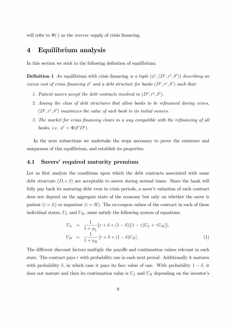
4.1 Savers’ required maturity premium

Let us first analyze the conditions upon which the debt contracts associated with some

debt structure (D, r, δ) are acceptable to savers during normal times. Since the bank will

fully pay back its maturing debt even in crisis periods, a saver’s valuation of such contract

does not depend on the aggregate state of the economy but only on whether the saver is

patient (i = L) or impatient (i = H). The ex-coupon values of the contract in each of these

individual states, UL and UH , must satisfy the following system of equations:

UL =1

1 + ρL{r + δ + (1− δ)[(1− γ)UL + γUH ]},

UH =1

1 + ρH[r + δ + (1− δ)UH ] . (1)

The different discount factors multiply the payoffs and continuation values relevant in each

state. The contract pays r with probability one in each next period. Additionally it matures

with probability δ, in which case it pays its face value of one. With probability 1 − δ, it

does not mature and then its continuation value is UL and UH depending on the investor’s

9

individual state in the next period. The terms multiplying these variables in the right hand

side of the equations reflect the probability of being in each individual state next period.

When banks place debt among savers, patient savers are abundant enough to acquire all

the issue, so the acceptability of the terms (r, δ) requires

UL(r, δ) =r + δ

ρH + δ

ρH + δ + (1− δ)γ

ρL + δ + (1− δ)γ≥ 1, (2)

which uses the solution for UL arising from (1). Obviously, for any given δ, bankers’ value is

maximized by issuing contracts with the minimal interest rate r that satisfies UL(r, δ) = 1.

Proposition 1 The minimal interest rate acceptable to patient savers for each maturity δ

is given by the function

r(δ) =ρHρL + δρL + (1− δ)γρH

ρH + δ + (1− δ)γ, (3)

which is strictly decreasing and convex, with r(0) = ρHρL+γρH+γ

∈ (ρL, ρH) and r(1) = ρL.

This result evidences the advantage of offering short debt maturities to the savers in our

model. For any expected maturity 1/δ longer than one, the saver bears the risk of turning

impatient and having to postpone his consumption until his contract matures. Compensating

the cost of waiting via a larger interest rate generates a maturity premium r(δ) − ρL > 0,

which is increasing in 1/δ. Figure 1 illustrates the behavior of r(δ) in a specific numerical

example.13

4.2 Banks’ optimal debt structures

From now on, we will take savers’ required maturity premium into account by assuming that

the debt structures (D, r, δ) offered by banks always have r = r(δ). This allows us to refer

banks’ debt structures as simply (D, δ). To further save on notation, in most equations we

will refer to r(δ) as simply r.

13All our figures rely on a baseline parameterization in which one period is one month, agents’ annualizeddiscount rates are ρL = 2% and ρH = 6%, the annualized yield on bank assets is μ = 4%, the expected timeuntil the arrival of an idiosyncratic preference shock is one year (γ = 1/12), and the expected time betweensystemic crises is ten years (ε = 1/120). We also assume Φ(x) = ax2, with a = 1 unless otherwise specified.

10

Figure 1: Interest rate spread vs. 1/δ

4.2.1 Value of bank equity in normal times

The continuation value of a bank to its owners in a normal period depends both on its

debt structure (D, δ) and the fraction α of its continuation value in a crisis that has to

be relinquished in order to obtain crisis financing. Let E(D, δ;α) denote the ex dividend

continuation value of the bank to its owners (i.e. the value of bank equity) in a normal period.

This value satisfies the following recursive equation:

E(D, δ;α) =1

1 + ρH

n(μ− rD) + (1− ε)E(D, δ;α) +

ε(1− α)1

1 + ρH[μ− (1− δ)rD + δD +E(D, δ;α)]

¾. (4)

To explain the equation, recall that bankers’ discount rate is ρH and after each normal period

they receive (and consume) a dividend of μ− rD.With probability 1− ε, the next period is

a normal period so bankers’ continuation value is E(D, δ;α) once again. With probability

ε, a systemic crisis arrives and refinancing the bank involves relinquishing a fraction α of its

equity value to the crisis financiers.

11

The factor 11+ρH

[μ− (1− δ)rD+ δD+E(D, δ;α)] represents the total value of the bank’s

equity after it gets financed in the crisis period. Such value is is expressed in terms of payoffs

received one period ahead: μ− (1− δ)rD is the asset cash flow net of interest payments to

savers (which reflects that the debt in hands of savers is temporarily reduced to (1−δ)D), δDis the revenue from reissuing the debt that was financed by experts during the crisis period

(paid as a special dividend to bank owners), and the last term reflects that, one period after

the crisis, the original debt structure is fully restored so the bank’s equity value is E(D, δ;α)

again.

Competition between crisis financiers implies that bankers will obtain the funds δD in

exchange for the minimal α that satisfies

α1

1 + ρH[μ− (1− δ)rD + δD +E(D, δ;α)] ≥ (1 + φ)δD. (5)

Under such α, (5) holds with equality and can be used to substitute for α in (4) and to

obtain the following Gordon-type formula for the value of bank equity value:

E(D, δ;φ) =1

ρH

∙μ− r(δ)D − ε

1 + ρH + ε{[(1 + ρH)φ+ ρH ]− r(δ)}δD

¸. (6)

The interpretation of this expression is very intuitive. Equity is valued as a perpetuity with

payoffs discounted at impatient rate ρH :

1. μ is the unlevered cash flow of the bank.

2. r(δ) is the interest rate paid on the debt placed among savers.

3. ε1+ρH+ε

{[(1+ρH)φ+ρH ]−r(δ)} reflects the (discounted) differential cost of refinancingthe amount of maturing debt δD each time a crisis arrives.

These elements provide the basis of our trade-off theory of banks’ debt structure decisions,

as shown in the sections below.

Finally, taking into account that (5) holds with equality and α cannot be larger than

one, the feasibility of crisis financing can be summarized by the condition:

μ− (1− δ)rD + δD +E(D, δ;φ) ≥ (1 + ρH)(1 + φ)δD, (7)

which we will call the crisis financing constraint (CF) in the analysis that follows. Quite

intuitively, the equity value of the bank after the crisis must be no lower than the amount

needed to compensate, at rate ρH , the cost 1 + φ of each unit of crisis financing.

12

4.2.2 Optimal debt structure problem

Since the bankers appropriate D out of what savers pay for the bank’s debt at t = 0, their

goal when choosing the bank’s initial debt structure is to maximize the total market value

of the bank, V (D, δ;φ) = D +E(D, δ;φ), which using (6) can be written as:

V (D, δ;φ) =μ

ρH+

ρH − r(δ)

ρHD − 1

ρH

ε(ρH − r(δ))

1 + ρH + εδD − 1

ρH

ε(1 + ρH)φ

1 + ρH + εδD. (8)

The first term in this expression is the value of the unlevered bank. The second term is the

value obtained by financing the bank with debt claims held by savers’ initially more patient

than the bankers (notice that r(δ) < ρH , by Proposition 1). The third term reflects the fact

that refinancing during crises is made by impatient experts whose discount rate is ρH instead

of by patient savers that require a yield r(). The last term accounts for the excess cost coming

from having to compensate all crisis financing according to the excess opportunity cost of

funds φ of the marginal crisis financier.

So bankers solve the following problem:

maxD≥0, δ∈[0,1]

V (D, δ;φ) = D +E(D, δ;φ)

s.t. E(D, δ;φ) ≥ 0 (LL)μ− (1− δ)rD + δD +E(D, δ;φ) ≥ (1 + ρH)(1 + φ)δD (CF)

(9)

The first constraint imposes the non-negativity of the bank’s equity value in normal periods,

and we will refer to it as bankers’ limited liability constraint (LL).14 The second constraint

is the crisis financing constraint (7), which can be interpreted as an expression of bankers’

limited liability in crisis times. It can be shown that the two constraints boil down to the

same constraint on D for δ = 0, but (CF) is tighter than (LL) for δ > 0.15 Thus (LL) can

be ignored.

Adopting the following technical assumptions help us prove the existence and uniqueness

of the solution to the bank’s optimization problem:16

A1. φ < 2 1+ρL1+ρH

− 1.

14Satisfying (LL) implies in particular the non-negativity of bankers dividends, μ− r(δ)D ≥ 0.15See the proof of Proposition 2 in Appendix A.16A1 and A2 are sufficient conditions that impose rather mild restrictions on the parameters. For instance,

in the baseline parameterization behind our figures (see footnote 13), A1 and A2 impose φ < 0.9936 andγ < 0.4976. Moreover, we have checked numerically that the results in Proposition 2 hold well beyond theregion of parameters delimited by these assumptions.

13

A2. γ < 1−ρH2

.

Proposition 2 The bank’s maximization problem has a unique solution (D∗, δ∗). In the

solution:

1. The crisis financing constraint is binding, i.e. crisis financiers take 100% of the bank’s

equity.

2. Optimal debt maturity 1/δ∗ is increasing in φ and the optimal amount of maturing debt

per period δ∗D∗ is decreasing in φ; in fact, if δ∗ ∈ (0, 1), both δ∗ and δ∗D∗ are strictly

decreasing in φ.

The intuition for these results is as follows. First, even if the bank does not get involved

in maturity transformation (δ = 0), its value is increasing in D, making it interested in

choosing the maximum feasible leverage. If maturity transformation generates value, this

tendency remains, so (CF) is binding at the optimum.17 Second, as the excess cost of crisis

financing φ increases, the value of maturity transformation diminishes which implies the

choice of a longer expected maturity. The tightening of (CF) forces banks to reduce the

amount of funding δ∗D∗ demanded to crisis financiers.18

Interestingly, the debt structure decisions just described determine, as a residual, the

bank’s capital ratio, that is, the ratio of its equity value E to its total market value V .

Figure 2 depicts E/V under banks’ optimal choices as a function of the excess cost of crisis

financing φ. The ratio is strictly increasing in φ, reflecting that, by (CF), each bank must

keep enough equity value in normal times so as to be able to pay the excess cost of funding

during a crisis.19 Under the illustrated parameterization, the model yields capital ratios in

a realistic 4% to 8% range for a wide range of values of φ.20

17The full dilution of bankers’ equity in each crisis is an implication of the simplifying assumption that allcrises have the same severity. With heterogeneity in this dimension (for example, due to random shifts inΦ(x)), the corresponding crisis financing constraint might only be binding (or even not satisfied, inducingbankruptcy) in the most severe crises.18In all our numerical examples, total debt D∗ is also decreasing in φ.19Even with φ = 0 banks need strictly positive equity because crisis financiers demand a return ρH larger

than r for their funds.20By construction, the capital ratios depicted in Figure 2 are the minimal ones compatible with banks

being able to avoid going bankrupt during a systemic liquidity crisis. These might be the relevant regulatorycapital ratios imposed on banks in an extended version of the model in which bankers did not want to avoidbankruptcy during crises (perhaps because they do not internalize some social costs of bank failures). SeeAppendix C for a discussion of the case in which banks default in crises.

14

Figure 2: Banks’ optimal capital ratio as a function of φ

4.3 The competitive equilibrium

Banks’ optimization problem for any given excess cost of crisis financing φ embeds savers’

participation constraint so the only condition for equilibrium that remains to be imposed is

the clearing of the market for crisis financing. The continuity and monotonicity in φ of the

function that describes excess demand in such market guarantees that there exists a unique

excess cost of crisis financing φe for which the market clears:

Proposition 3 The equilibrium of the economy (φe, (De, re, δe)) exists and is unique.

The effects on equilibrium outcomes of shifts in the supply of crisis financing are sum-

marized in the following proposition:

Proposition 4 If the inverse supply of crisis financing Φ(x) shifts upwards, the equilibrium

changes as follows: expected debt maturity 1/δe increases, total refinancing needs δeDe fall,

bank debt yields re increase, and the excess cost of crisis financing φe increases. If initially

δe ∈ (0, 1), all these variations are strict.

15

Figure 3: Effect of changes in the parameters on the competitive equilibrium

The results in Proposition 4 are illustrated, together with other comparative statics re-

sults, in Figure 3, where the inverse supply of crisis financing is parameterized asΦa(x) = ax2.

The graphs in the first column plot various equilibrium variables (expected debt maturity,

total debt, and excess cost of crisis financing) against the parameter a of this function. The

second and third columns show the equilibrium effects of increasing the average time to the

arrival of a systemic shock, 1/ε, and an idiosyncratic shock, 1/γ, respectively. These results

are quite self-explanatory.

5 Efficiency and regulatory implications

In this section we solve the problem of a social planner who has the ability to control banks’

funding decisions subject to the same constraints that banks face when solving their private

16

value maximization problems. We find that bank debt maturity in the unregulated compet-

itive equilibrium is inefficiently short because of the interaction of a pecuniary externality

with banks’ crisis financing constraints. We find that banks’ endogenous continuation values

amplify the significance of the inefficiency. Finally, we analyze two specific alternatives that

would restore efficiency: directly regulating maturity decisions and the introduction of a

suitable Pigovian tax on banks’ refinancing needs.

5.1 Inefficiency of the unregulated equilibrium

Suppose that a social planner can regulate both the amount D and the maturity parameter δ

of banks’ debt. In our economy only existing bankers and future crisis financiers appropriate

a surplus. So the natural objective function for the social planner is the sum of the present

value of such surpluses. Crisis financiers appropriate the difference between the equilibrium

excess cost of crisis financing, φ = Φ(δD), and the net present value of their alternative

investment opportunity z (which is positive for all but the marginal crisis financiers). Hence,

crisis financiers’ surplus is:

u(D, δ) =

Z δD

0

(Φ(δD)− Φ(x)) dx = δDΦ(δD)−Z δD

0

Φ(x)dx. (10)

Evaluated at a normal period, the present value of the expected surpluses of potential crisis

financiers along future crises can be written as:21

U(D, δ) =1

ρH

(1 + ρH)ε

1 + ρH + εu(D, δ).

Hence, using (8), the objective function of the social planner can be expressed as:

W (D, δ) = V (D, δ;Φ(δD)) + U(D, δ)

=μ

ρH+

ρH—r(δ)ρH

D − 1

ρH

ε(ρH—r(δ))1+ρH+ε

δD − 1

ρH

(1 + ρH)ε

1+ρH+ε

Z δD

0

Φ(x)dx, (11)

21U(D, δ) satisfies the following recursive equation:

U(D, δ) =1

1 + ρH

∙(1− ε)U(D, δ) + ε

µu(D, δ) +

1

1 + ρHU(D, δ)

¶¸.

The first term in square brackets takes into account that, with probability 1 − ε, next period is a normalone and crisis financiers’ continuation surplus remains equal to U(D, δ). The second term captures that withprobability ε there is a crisis and the crisis financiers obtain u(D, δ) plus the continuation surplus that, onemore period ahead, is again U(D, δ).

17

which contains four terms: the value of an unlevered bank, the value added by maturity

transformation in the absence of systemic crises, the value loss due to financing the bank

with impatient experts during liquidity crises, and the value loss due to the sacrifice of the

NPV of the investment projects given up by those experts who act as banks’ crisis financiers.

Thus, the social planner’s problem can be written as:22

maxD≥0, δ∈[0,1]

W (D, δ)

s.t. μ—(1—δ)rD+δD+E(D, δ;Φ(δD)) ≥ (1+ρH)(1+Φ(δD))δD (CF’)

(12)

This problem differs from banks’ optimization problem (9) in two dimensions. First, the

objective function includes the surplus of the crisis financiers. Second, the social planner

internalizes the effect of banks’ funding decisions on the market-clearing excess cost of crisis

financing, so (CF’) contains Φ(δD) in the place occupied by φ in (CF) constraint (see problem

(7)).

Comparing the unregulated equilibrium with the solution of the social planner’s problem,

we obtain the following result:

Proposition 5 If the competitive equilibrium features δe ∈ (0, 1) then a social planner canincrease social welfare by choosing a longer expected debt maturity than in the competitive

equilibrium, i.e. some 1/δs > 1/δe.

The root of the discrepancy between the competitive and the socially optimal allocations

is at the way individual banks and the social planner perceive the frontier of the set of

maturity transformation possibilities: banks choose their individually optimal (D, δ) along

the (CF) constraint (where φe is taken as given) whereas the social planner does it along

the (CF’) constraint (where φ = Φ(δD)). Each of these constraints and the corresponding

decisions are illustrated in Figure 4.

At the equilibrium allocation (De, δe) both the social planner’s and the initial bankers’

indifference curves are tangent to (CF). Moreover, (CF) and (CF’) intersect at (De, δe) (since

the competitive equilibrium obviously satisfies φe = Φ(δeDe)). However, the social planner’s

indifference curve is not tangent to (CF’) at (De, δe), implying that this allocation does not

maximize welfare. In the neighborhood of (De, δe), (CF’) allows for a larger increase in D,

22Recall that the constraint called (LL) in (9) can be ignored because it is implied by the bridge financingconstraint.

18

Figure 4: Maturity transformation possibilities from private and social perspectives

by reducing δ, than what seems implied by (CF) (where φ remains constant). It turns out

that maturity transformation can produce a larger surplus with a larger use of its extensive

margin (leverage) and a lower use of its intensive margin (short maturities), like at (Ds, δs)

in the figure.

This finding offers a new perspective for the joint assessment of some of the regulatory

proposals emerged in the aftermath of the recent crisis, which defend reducing both banks’

leverage and their reliance on short-term funding. In the context of the current model, once

debt maturity is regulated, limiting banks’ leverage would be counterproductive. It also

indicates that simply limiting banks’ leverage (say, through higher capital requirements)

does not correct, and would actually worsen, the impact of the externality associated with

refinancing needs. In terms of Figure 4, forcing banks to choose debt lower than De would

induce them to, in the new regulated equilibrium, move along (CF’) in the direction that

implies a larger δ, i.e. a shorter expected debt maturity, and lower aggregate welfare.

19

5.2 Amplification via continuation value

The source of inefficiency in our model is the impact on banks’ financing constraints of

pecuniary externalities generated in the market for crisis financing. As in Stein (2012),

where the pecuniary externalities operate through asset sales, the unregulated equilibrium

involves excessive refinancing needs. An important difference between both papers is that in

our infinite horizon model crises are recurrent and the continuation value of a bank depends

on the anticipated cost of funds in future crises. In our setup, reducing banks’ refinancing

needs reduces the excess cost of financing in each future crisis, φ, producing two effects that

the social planner problem internalizes (but banks do not): (i) the direct effect of φ on the

RHS of (CF’); and (ii) the indirect effect of φ on banks’ continuation value in a crisis and,

hence, on the LHS of (CF’). The second effect emanates from our recursive formulation and

reinforces the first in relaxing (CF’).

In order to quantify the importance of each effect we conduct the following exercise. We

consider a social planner that only regulates debt structures up to the arrival of the first crisis.

For the sake of the calculation, at the normal period following the first crisis, we allow banks

to repay all their debt and reissue debt under the structure that is optimal in the unregulated

equilibrium. The recursive equations that determine the market value of banks, the relevant

crisis financing constraint, the rents obtained by crisis financiers and, henceforth, the problem

of the one-off (rather than recursive) social planner are developed in Appendix B. Figure

5 compares expected debt maturity and total debt across the unregulated equilibrium and

the one-off and recursive regulated equilibria. Clearly, regulated maturities and total debt

are larger in the recursive welfare problem than in the one-off problem, and the size of the

differences in total debt (which is the source of the initial dividend through which bankers

appropriate the surplus from maturity transformation) suggests that the effects channeled

through banks’ continuation value are quantitatively very important.23

23In terms of Figure 4, the recursive planner’s impact on bank continuation value implies that the frontierof maturity transformation possibilities over which he optimizes, (CF’), is steeper around (De, δe) thanthe frontier relevant to the one-off planner (which would, in turn, be steeper than banks’ crisis financingconstraint, (CF)).

20

Figure 5: Competitive equilibrium vs. socially-efficient funding structures

5.3 Restoring efficiency

In order to achieve the socially efficient debt structure (Ds, δs) as a regulated competitive

equilibrium, the most straightforward intervention in the context of the model would be

to impose an upper limit δs to banks’ maturity decision δ. Given that the inverse of δ is

the expected maturity of a bank’s debt (and our banks’ assets have infinite maturity), such

limit could be interpreted as equivalent to introducing a minimum net stable funding ratio

like the one considered in Basel III. Anticipating a cost of crisis financing φs, banks in our

model would find such a requirement binding and would choose to issue the maximum debt

compatible with (CF) given φs and δs, which is Ds.

As shown by Perotti and Suarez (2011), adding unobservable heterogeneity across banks

may undermine the efficiency of one-size-fits-all quantity-based liquidity regulation and al-

21

ternatives such as Pigovian taxes may be superior.24 With this motivation in perspective

(but without explicitly adding heterogeneity), we next check whether a Pigovian tax on

banks’ refinancing needs might implement (Ds, δs) as a regulated competitive equilibrium.

We consider the following class of non-subsidized Pigovian schemes:

1. Each bank pays a proportional tax of rate τ per period on its refinancing needs δD.

2. The social planner pays to each bank a lump-sum transfer M ≤ τδD per period.

Since τδD is the revenue from the Pigovian tax, the constraint M ≤ τδD rules out the

possibility of subsidizing banks via the lump-sum transfer M.We can prove analytically the

following result:

Proposition 6 If the unregulated competitive equilibrium features δe ∈ (0, 1), there existsa Pigovian tax scheme (τP ,MP ) that induces the socially optimal allocation (Ds, δs). This

scheme satisfies τP > 0 and MP = τP δsDs, and is unique if δs > 0.

The scheme uses some τP > 0 to push banks towards funding decisions involving lower

refinancing needs than in the unregulated competitive equilibrium. Interestingly, in order to

reach the socially efficient allocation, all the revenue raised by the tax τP has to be rebated to

the banks through MP . Values of τ and M which induce δs but involve M < τδPDP would

reduce the value of bank equity relative to the situation in which δs is directly regulated,

which would in turn tighten banks’ crisis financing constraint pushing banks towards a

leverage DP strictly lower than Ds.

The need for rebating the revenue from the Pigovian tax is a novel insight relative to

the non-pecuniary externality setup of Perotti and Suarez (2011). The general intuition is

that, when pecuniary externalities cause inefficiency due to their interaction with financial

constraints, regulators must be cautious not to address one of the manifestations of the

inefficiency (excessively short maturities) in a way (non-rebated taxes) that, by tightening

the relevant constraints (here, reducing banks’ continuation values) may partly undo the

potential gains from the intervention.

24Specifically, these authors show that if banks unobservably differ in their opportunities to extract valuefrom maturity transformation, a flat rate Pigovian tax on refinancing needs can induce the marginal inter-nalization of the relevant externalities while allowing the most efficient banks to operate with larger maturitymismatches than the less efficient ones.

22

6 Liquidity insurance

Some recent discussions on the final shape of bank liquidity risk regulation suggest the need

to consider in parallel the possibility that banks’ refinancing needs in a crisis are covered

by explicit liquidity insurance schemes (Stein, 2013). In the next two subsections we con-

sider the potential welfare contribution of private and government-based liquidity insurance

arrangements. In both parts we conclude that liquidity insurance is socially beneficial but

does not eliminate the desirability of debt maturity regulation, the intensity of which should

generally depend, among other things, on the price elasticity of the opportunity cost of

insurers’ funds.

6.1 Private liquidity insurance

The fact that in both the competitive and the regulated allocations banks’ crisis financing

constraints are binding, while the normal times limited liability constraints are not, suggests

that some form of insurance against systemic liquidity crises might increase welfare. To

keep things tractable, we focus on simple one-period refinancing insurance arrangements

subscribed by individual banks and entering experts at the beginning of each period, prior

to the realization of uncertainty regarding the occurrence of a crisis.

Specifically, the arrangements we consider establish that:

1. Except in the period immediately after each crisis,25 the bank pays a per-period pre-

mium p for each unit of insured refinancing λδD > 0 to a measure λδD of entering

experts, where λ ∈ [0, 1] is the insured fraction of refinancing needs.

2. If there is a systemic crisis, the insuring experts supply the bank with funds λδD in

the crisis and receive a gross repayment of [1 + r(δ) + p]λδD just after the crisis.

Under this arrangement the refinancing of λδD is just as costly as if no crisis had occurred

(r(δ) is the normal yield of savers’ debt). The part pλδD of the repayment to the insuring

experts after the crisis is included to offset the impact on the banks’ net income of the fact

that insurance is unneeded (and hence not paid for) immediately after a crisis.

25Insurance in the period immediately after a crisis is unneeded because, according to our assumptions,crisis periods are always followed by a normal period.

23

For the sale of insurance to be attractive to an entering expert with funds that can earn

NPV of z in normal periods and max{z, φ} in crisis periods, the insurance premium p must

satisfy

p+ ε1 + r + p

1 + ρH≥ εmax{1 + z, 1 + φ}, (13)

where the second term in the LHS is the present value of the post-crisis repayments described

above. Competition among entering experts will lead to a situation in which (13) is binding

for the marginal provider of either insurance or crisis financing, who will have z = φ.26

Solving for p in such equality yields

p =ε

1 + ρH + ε{[(1 + ρH)φ+ ρH ]− r(δ)}, (14)

which is identical to the factor (within the large square brackets) that multiplies δD in (6).

On the other hand, the value of equity in a normal period of a bank that decides to insure

a fraction λ of its refinancing needs can be written as

E(D, δ, λ;φ) =1

ρH

½μ− r(δ)D − pλδD − ε

1+ρH+ε{[(1 + ρH)φ+ ρH ]− r(δ)}(1—λ)δD

¾,

which is an extended version of (6). Now, using (14) to substitute for p, it becomes clear

that:

E(D, δ, λ;φ) = E(D, δ, 0;φ) = E(D, δ;φ), (15)

which can be interpreted as a Modigliani-Miller type result: moving the fraction λ of fairly-

priced insured funding for given value of D and δ, does not per se create or destroy value..

Insurance is, however, relevant for the bank’s overall optimization problem because it

alters the bank’s crisis financing constraint. In the presence of insurance, the crisis financing

constraint can be written as:

(μ−λpδD)− [1− (1−λ)δ]rD+(1−λ)δD+E(D, δ;φ) ≥ (1+ρH)(1+φ)(1−λ)δD, (CFI)

which differs from (7) in the presence of the insurance premia subtracting from the cash

flow and adaptations that reflect that the bank’s effective refinancing needs in the crisis are

reduced to the uninsured fraction of its debt, (1− λ)δD.

26Clearing the market for crisis financing requires φ = Φ(δD) irrespectively of the fraction of δD coveredwith insurance.

24

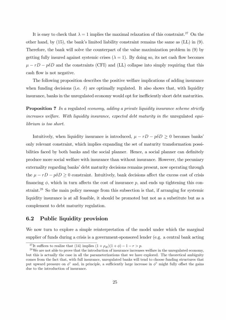
It is easy to check that λ = 1 implies the maximal relaxation of this constraint.27 On the

other hand, by (15), the bank’s limited liability constraint remains the same as (LL) in (9).

Therefore, the bank will solve the counterpart of the value maximization problem in (9) by

getting fully insured against systemic crises (λ = 1). By doing so, its net cash flow becomes

μ − rD − pδD and the constraints (CFI) and (LL) collapse into simply requiring that this

cash flow is not negative.

The following proposition describes the positive welfare implications of adding insurance

when funding decisions (i.e. δ) are optimally regulated. It also shows that, with liquidity

insurance, banks in the unregulated economy would opt for inefficiently short debt maturities.

Proposition 7 In a regulated economy, adding a private liquidity insurance scheme strictly

increases welfare. With liquidity insurance, expected debt maturity in the unregulated equi-

librium is too short.

Intuitively, when liquidity insurance is introduced, μ − rD − pδD ≥ 0 becomes banks’only relevant constraint, which implies expanding the set of maturity transformation possi-

bilities faced by both banks and the social planner. Hence, a social planner can definitely

produce more social welfare with insurance than without insurance. However, the pecuniary

externality regarding banks’ debt maturity decisions remains present, now operating through

the μ− rD − pδD ≥ 0 constraint. Intuitively, bank decisions affect the excess cost of crisisfinancing φ, which in turn affects the cost of insurance p, and ends up tightening this con-

straint.28 So the main policy message from this subsection is that, if arranging for systemic

liquidity insurance is at all feasible, it should be promoted but not as a substitute but as a

complement to debt maturity regulation.

6.2 Public liquidity provision

We now turn to explore a simple reinterpretation of the model under which the marginal

supplier of funds during a crisis is a government-sponsored lender (e.g. a central bank acting

27It suffices to realize that (14) implies (1 + ρH)(1 + φ)− 1− r > p.28We are not able to prove that the introduction of insurance increases welfare in the unregulated economy,

but this is actually the case in all the parameterizations that we have explored. The theoretical ambiguitycomes from the fact that, with full insurance, unregulated banks will tend to choose funding structures thatput upward pressure on φe and, in principle, a sufficiently large increase in φe might fully offset the gainsdue to the introduction of insurance.

25

as a lender of last resort) which is constrained to offer its funds on a non-subsidized basis.

Specifically, suppose that the supply of funds from entering experts in a crisis is too small,

say zero, but the government is able to obtain alternative funds x with a marginal (excess)

opportunity cost that, to save on notation, we describe with the function Φ(x), which is

analogous to our previous inverse supply of crisis financing.29

We are going to compare two public liquidity insurance regimes in which the government

commits to cover, on a non-subsidized basis, banks’ crisis financing needs:30

I. Public liquidity insurance only In each period, the government charges an in-

surance premium pδD to each bank with refinancing needs δD and commits to cover these

needs in each crisis period in exchange for a repayment of [1 + r(δ)]δD in the period after

the crisis.31

II. Public liquidity insurance cum maturity regulation In addition to the arrange-

ments of the previous regime, the government regulates banks’ maturity decision δ.

As with private insurance, banks’ optimal debt structure decisions maximize the total

market value of the bank (like in (9)), but only subject to the limited liability constraint

μ− rD− pδD ≥ 0. The NPV of the revenues and costs that accrue to the government in itsrole as an insurer are:

G =1

ρH

∙pδD − ε (ρH − r(δ))

1 + ρH + εδD − (1 + ρH)ε

1 + ρH + ε

Z δD

0

Φ(x)dx

¸, (16)

where the last term accounts for the (excess) opportunity cost of the funds lent in a crisis.

Aggregate welfare in this setting can be defined as the sum of the total market value of

the insured banks, V, and the net present value of the government’s stake, G. The resulting

expression for welfare is analogous to the expression for W in (11). We assume that the

government maximizes W, subject to G ≥ 0, i.e. we do not allow for positive NPV transfers29We refer to Φ(x) as an excess cost because it comes on top of the normal opportunity cost of funds

implied by assuming that the government has the same discount rate ρH as impatient agents. This excesscost may here reflect the NPV of the deadweight losses due to future distortionary taxes.30The government might instead commit to supply liquidity during crises at some fixed excess cost bφ à la

Bagehot (1873). Numerical simulations show that this alternative policy is dominated by the arrangementsthat we analyze. The reason is that, as in the case of private liquidity insurance analyzed above, spreadingthe excess cost of crisis liquidity over time expands the set of maturity transformation possibilities.31For simplicity, we assume that pδD is paid to the government in every period (including periods after a

crisis where the probability of suffering another crisis is zero).

26

from the government to the bank owners.32

The difference between the two public liquidity insurance regimes described above stems

from the tools through which the government may influence banks’ decisions. In Regime

I, the government can only set p and will do so taking into account the impact of p on

(D, δ) = (D(p), δ(p)). So, in this regime the premium p has to play the dual role of regulating

banks’ refinancing needs δD and guaranteeing G ≥ 0. In Regime II, the government can setboth p and δ, taking into account the impact of both parameters on (D, δ) = (D(p, δ), δ),

and it turns out that the second tool is useful too. In fact, when the only tool is p, the

welfare maximizing solution involves G > 0 in all our simulations while, when the two tools

are available, it is possible to prove that the optimum involves G = 0.

Based on the same underlying parameterization as in previous figures, Figure 6 illustrates

the outcomes under each of the two commented regimes. The horizontal axes represent dif-

ferent excess costs of government funds, measured by the factor a of a cost function specified

as Φ(x) = ax. Panel A represents welfare gains relative to a benchmark scenario without

liquidity insurance in which banks fail if they have refinancing needs during a crisis.33 These

gains decrease as the excess cost of government funds increases and are significantly greater

when maturity regulation is allowed. Quite intuitively, expected debt maturity (depicted

in Panel B) is shorter when it can only be regulated using the premium p than when δ is

controlled by the regulator. Finally, Panel C shows the positive government surplus G > 0

associated with Regime I and the zero surplus G = 0 associated with Regime II.34

As in the case of private liquidity insurance, the results in this subsection deliver the

message that liquidity insurance is not a substitute but a complement to maturity regula-

tion. With or without liquidity insurance, unregulated banks tend to choose equilibrium

debt maturities that are excessively short, in that they imply refinancing costs during crises

that tighten banks’ financial constraints and impede them to collectively provide maturity

32Notice that this constraint is more flexible than the constraint associated with private liquidity insurance,where the marginal (rather than the average) provider of insurance must break even.33The liquidation value L in case of default has been calibrated so that it equals 80% of the total market

value of the bank. This choice only affects the scale of the vertical axis in Panel A. Details about the casein which banks fail in crises are provided in Section 7.1 and Appendix C.34Consistent with the result in Proposition 6, a solution based on the combination of Pigovian taxes and

lump-sum rebates might replace the direct regulation of δ. The resulting Pigovian insurance scheme wouldcharge an excess insurance premium so as to induce the same maturity decision as the one directly regulatedin Regime II and it would then rebate the government surplus to the banks in a periodic manner so as tocompensate the negative effects of the excessive premia on equity values.

27

Figure 6: Optimal policy interventions vs. the government cost of funds

transformation in the socially most valuable manner.

7 Discussion and extensions

In this section we comment on the key assumptions and possible extensions of our model.

7.1 Optimality of not defaulting during crises

We have so far assumed that the liquidation value of banks in case of default, L, is small

enough for banks to find it optimal to rely on funding structures that satisfy the (CF)

constraint. How small L has to be (and what happens if it is not) is discussed next.

If a bank were not able to refinance its maturing debt, it would default, and we assume

that this would precipitate its liquidation. For simplicity, we assume that, if the bank

defaults, the liquidation value L is orderly distributed among all debtholders, which excludes

the possibility of preemptive runs à la He and Xiong (2011a). If a bank were expected to

default in a crisis, savers would require r to include a compensation for credit risk.

Based on the derivations provided in Appendix C, Figure 7 depicts for each possible

equilibrium excess cost of crisis financing, φe, the maximum liquidation value Lmax(φe) for

28

Figure 7: Conditions for the optimality of not defaulting during crises

which, when all other banks opt for crisis financing, an individual bank also prefers to rely on

crisis financing. The variation of φe in this figure can be thought of as a general representation

of shifts in the inverse supply of crisis financing Φ(δD) (which only affects the banks opting

for crisis financing) so that both dimensions of the figure account for shifts in exogenous

parameters. For configurations of parameters with L ≤ Lmax(φe), the candidate equilibrium

with crisis financing gets confirmed as an equilibrium.

Lmax(φe) is decreasing, so the higher the excess cost of crisis funding, the stronger the

incentives for banks to opt for funding structures that imply defaulting in a crisis. To

reinforce intuitions, Figure 7 also shows the total market value in a crisis of a bank that relies

on crisis financing, V C(φe).35 The fact that V C(φe) > Lmax(φe) reflects that, for the values

of L contained between the two curves, liquidation in case of a crisis is ex-post inefficient.

Yet, opting for liquidation in a crisis, the bank can get rid of the (CF) constraint in (9) and

expand its leverage up to the level allowed by (LL), so bankers may find it ex-ante optimal.

In situations with L > Lmax(φe) at least some banks will opt for being exposed to

35Since (CF) is binding, the value of a bank’s pre-existing equity at a crisis is 0 and thus V C(φe) = De(φe).

29

liquidation during each systemic crisis. Given the absence of new bank formation in our

model, one may wonder whether such a configuration of parameters would lead to the full

collapse of the banking sector after sufficiently many crisis. However, for L < Lmax(0), the

answer is no, since there is a self-equilibrating mechanism: Bank exit will adjust φ down

after each crisis, leading to a steady state in which all surviving banks eventually rely on

crisis financing.36 So for L < Lmax(0), the type of equilibrium with crisis financing on which

we have focused in the main sections of the paper is the long term equilibrium of the banking

industry.

7.2 Deterministic vs random maturity

For tractability we have assumed that debt contracts have random maturity. It would be

more realistic to assume that the bank chooses an integer T that describes the deterministic

maturity of its debt contracts. In this setting it is possible to determine savers’ required

maturity premium rdet(T ) as we did in Section 4.1. It can also be shown that for T = 1/δ,

we have rdet(T ) < r(δ) because discounting is a convex function of time and thus the random

variation in maturity realizations produces disutility to impatient savers.

With deterministic maturities, the model would lose some of the Markovian properties

that make it tractable. In the period after a crisis the initial funding structure would not be

immediately reestablished since, in addition to the debt with principal 1TD that matures and

has to be refinanced, the bank would also have to issue the debt with face value 1TD that

was bridge financed during the crisis. Thus, in order for the bank to keep a constant fraction

1/T of debt maturing in each period, half of the debt issued by the bank in the after-crisis

period should have maturity T − 1, but this would introduce heterogeneity in interest ratepayments across the various debts. The description would become further complicated if a

new crisis arrives prior to the maturity of the debt with maturity T − 1.Therefore, assuming random maturities implies some loss of banks’ value but is essential

to the simplicity of our recursive valuation formulas. However, there is no reason to think

that deterministic rather than random maturities would qualitatively change any of the

36In such an equilibrium the mass of banks would be m < 1 and the excess cost of crisis financing wouldequal the unique φm that satisfies Lmax(φm) = L. Now, if (Dm, δm) denotes the funding decision under φm ofbanks subject to the (CF) constraint, thenm can be found as the unique value that solves Φ(mδmDm) = φm.If the mass of banks were at any point larger than m, then a mass m of banks would use (Dm, δm), survivingeach crisis, while the remaining ones would be exposed to liquidation in each crisis.

30

trade-offs behind the key results of the paper.

7.3 Resetting debt structures over time

For the sake of clarity, we have assumed that the debt structure (D, δ) decided at t = 0 is

kept constant over normal periods and restored immediately after each crisis. What would

happen if bankers could re-optimize in periods different from t = 0?

To narrow down the question, suppose, in particular, that outstanding debt were exoge-

nously (and unexpectedly) maturing all at a time in a single normal period and bankers

were allowed to decide a new debt structure from thereon. It is obvious from the Markovian

structure of the model that their optimal decision would coincide with the initial one.37

The more general case in which at every date the bank could decide to roll-over part of

its maturing debt at perhaps some new terms, while keeping constant the structure of its

non-maturing debt, is hard to analyze because describing the debt structures that a bank

might end up having requires a very complicated space of state variables. However, we find

no obvious reasons to expect that those more general funding structures would increase the

value to the bank. Intuition from simpler models suggests that altering the terms of new

debt as maturing debt is rolled over might only create value to shareholders at the expense

of non-maturing debt holders, but this (i) would have a negative repercussion on the value of

such a debt when issued (and hence on initial shareholder value) and (ii) could be prevented

by including proper covenants in the preexisting debt contracts.38

7.4 Tradability of debt

The non-tradability of banks’ debt plays a key role in the model. Savers who turn impatient

suffer disutility from delaying consumption until their debt matures because there is no

secondary market where to sell the debt (or where to sell it at a sufficiently good price).

If bank debt could be traded without frictions, impatient savers would sell their debts to

37The formal argument goes as follows: denote the bank’s current debt structure by (D, δ). In a N statethat does not follow a C state, the market value of total outstanding debt is D. Current shareholders wouldmaximize V (D, δ;φ) − D subject to the same financing constraints as at t = 0 and the optimal solutionwould be the same as at t = 0, since the only difference between the initial optimization problems and thecurrent one is the (constant) D now subtracted from the objective function. In a N state that follows a Cstate, the market value of outstanding debt would be (1 − δ)D and current shareholders would maximizeV (D, δ;φ)− (1− δ)D but again the solution would not change.38See Brunnermeier and Oehmke (2013).

31

patient savers. Banks could issue perpetual debt (δ = 0) at some initial period and get

rid of refinancing concerns. In practice a lot of bank debt, starting with retail deposits,

but including also certificates of deposit placed among the public, interbank deposits, debt

involved in sales with repurchase agreements (repos), and commercial paper are commonly

issued over the counter (OTC) and have no liquid secondary market.

Our model does not contain an explicit justification for the lack of tradability. Arguably,

it might stem from administrative, legal compliance, and operational costs associated with

the trading (specially using centralized trade) of heterogenous debt instruments issued in

small amounts, with a short life or among a dispersed mass of unsophisticated investors. In

fact, if other banks (or some other sophisticated traders) could possess better information

about banks than ordinary savers, then costs associated with asymmetric information (e.g.

exposure to a winners’ curse problem in the acquisition of bank debt) might make the

secondary market for bank debt unattractive to ordinary savers (Gorton and Pennacchi,

1990). This view is consistent with the common description of interbank markets as markets

where peer monitoring is important (Rochet and Tirole, 1996).

Additionally, the literature in the Diamond and Dybvig (1983) tradition has demon-

strated that having markets for the secondary trading of bank claims might damage the

insurance role of bank deposits.39 Yet, Diamond (1997) makes the case for the complemen-

tarity between banks and markets when, at least for some agents, the access to markets is

not guaranteed.

Our model could be extended to describe situations in which debt is tradable but in

a non-centralized secondary market characterized by search frictions (like in the models

of OTC markets recently explored by Duffie, Gârleanu, and Pedersen, 2005, Vayanos and

Weill, 2008, and Lagos and Rocheteau, 2009). In such setting, shortening the maturity of

debt would have the effect of increasing the outside option of an impatient saver who is

trying to find a buyer for his non-matured debt.40 This could allow sellers to obtain better

prices in the secondary market, making them willing to pay more for the debt in the first

place and encouraging banks to issue short-term debt.41

39See von Thadden (1999) for an insightful review of the results obtained in this tradition.40He and Milbradt (2012) and Bruche and Segura (2013) explicitly model the secondary market for cor-

porate debt as a market with search frictions.41In Bruche and Segura (2013), these trade-offs imply a privately optimal maturity for bank debt. The

empirical evidence in Mahanti et al. (2008) and Bao, Pan, and Wang (2011), among others, shows that

32

8 Conclusion

We have developed an infinite horizon equilibrium model in which banks with long-lived

assets decide the overall principal, interest rate payments, and maturity of their debt (and,

as residual, their equity financing). Savers’ preference for short maturities comes from their

exposure to idiosyncratic preference shocks and the lack of tradability of bank debt. Banks’

incentive not to set debt maturities as short as savers might ceteris paribus prefer, comes

from the fact that there are episodes (systemic liquidity crises) in which their access to savers’

funding fails and their refinancing becomes more expensive.

We identify a pecuniary externality in the market for crisis financing that, when com-

bined with the financial constraints faced by banks, renders the unregulated competitive

equilibrium socially inefficient. It turns out that, if a social planner coordinates the banks in

the choice of longer debt maturities, then banks’ total leverage and the social value of their

overall maturity transformation activity increases.

We have explored alternatives for restoring efficiency, including forcing banks to issue

debt of longer maturities or inducing them to do so with a Pigovian tax on their refinancing

needs. We have assessed the amplifying impact of banks’ endogenous continuation values

on the size of the inefficiency and the impact of regulation. We have also considered the

implications of adding private or public liquidity insurance schemes, finding that the case for

regulating maturity decisions does not disappear, so that liquidity insurance and liquidity

risk regulation can be considered complements rather than substitutes in dealing with the

systemic liquidity risk.

short-term bonds are indeed more “liquid” (as measured by the narrowness of the bid-ask spread) thanlong-term bonds.

33

Appendix

A Proofs

This appendix contains the proofs of the propositions included in the body of the paper.

Proof of Proposition 1 Using (3) it is a matter of algebra to obtain that:

r0(δ) =−γ(1 + ρH)(ρH − ρL)

{ρH + δ + (1− δ)γ}2 < 0,

r00(δ) =2γ (1− γ) (1 + ρH)(ρH − ρL)

{ρH + δ + (1− δ)γ}3 > 0.

The other properties stated in the proposition are immediate.¥

Proof of Proposition 2 The proof is organized in a sequence of steps.

1. If (CF) is satisfied then (LL) is strictly satisfied Using equation (6) we have that(LL) can be written as:

0 ≤ E(D, δ;φ) =1

ρH(μ− rD)− 1

ρH

(1 + ρH)ε

1 + ρH + ε

µ1 + φ− 1 + r

1 + ρH

¶δD,

while (CF) can be written, using (7), as

0 ≤ 1

1 + ρH[μ− r(1− δ)D + δD +E(D, δ;φ)]− (1 + φ)δD =

=1

ρH(μ− rD)−

µ1 +

1

ρH

ε

1 + ρH + ε

¶µ1 + φ− 1 + r

1 + ρH

¶δD.

Now, since 1 + 1ρH

ε1+ρH+ε

> (1+ρH)ερH(1+ρH+ε)

we conclude that whenever (CF) is satisfied, (LL) isstrictly satisfied.

2. Notation and useful bounds Using equation (6) we can write:

V (D, δ;φ) = D +E(D, δ;φ) =1

ρHμ+DΠ(δ;φ),

where

Π(δ, φ) = 1− 1

ρH

∙µ1− ε

1 + ρH + εδ

¶r +

(1 + ρH)ε

1 + ρH + εδ

µφ+

ρH1 + ρH

¶¸can be interpreted as the value the bank generates to its shareholders per unit of debt. UsingProposition 1 we can see that the function Π(δ, φ) is concave in δ.

34

(CF) in equation (7) can be rewritten as:

μ+ V (D, δ;φ) ≥ [(1 + ρH)(1 + φ)δ + (1 + r)(1− δ)]D,

and if we define C(δ, φ) = (1+ρH)(1+φ)δ+(1+ r)(1− δ), (CF) can be written in the morecompact form that will be used from now onwards:

1 + ρHρH

μ+ [Π(δ, φ)− C(δ, φ)]D ≥ 0. (17)

Using Proposition 1 we can see that the function C(δ, φ) is convex in δ.

We have the following relationship:

Π(δ, φ) = 1− 1

ρH

1 + ρH1 + ρH + ε

∙r(δ) +

ε

1 + ρH(C(δ, φ)− 1)

¸(18)

Assumption A1 implies (1 + ρH)(1 + φ) ≤ 2(1 + ρL) ≤ 2(1 + r(δ)) for all δ, and we cancheck that the following bounds (that are independent from φ) hold:

C(δ, φ) ≥ 1 + r(δ).

∂C(δ, φ)

∂δ≤ 2(1 + r(δ))− (1 + r(δ)) = 1 + r(δ). (19)

Using assumption A2, it is a matter of algebra to check that, for all δ,

d2r

dδ2+

dr

dδ≥ 0.

And, from this inequality, drdδ

< 0, and r < ρH , it is possible to check that:

∂2Π(δ, φ)

∂δ2+

∂Π(δ, φ)

∂δ< − 1

ρH

µ1− ε

1 + ρH + εδ

¶µdr

dδ+

d2r

dδ2

¶≤ 0. (20)

To save on notation, we will drop from now on the arguments of these functions when itdoes not lead to ambiguity.

3. D∗ = 0 is not optimal It suffices to realize that ∂V (D,0;φ)∂D

= Π(0, φ) = 1− r(0)ρH

> 0.

4. The solution (D∗, δ∗) of the maximization problem in equation (9) exists, isunique, and satisfies (CF) with equality, i.e. 1+ρH

ρHμ+ (Π(δ∗, φ)− C(δ∗, φ))D∗ = 0

We are going to prove existence and uniqueness in the particular case that there existδΠ, δC ∈ [0, 1] such that ∂Π(δΠ,φ)

∂δ= ∂C(δC ,φ)

∂δ= 0. This will ensure that the solution of the

maximization problem is interior in δ. The other cases are treated in an analogous way butmight give rise to corner solutions in δ.42

42More precisely, if for all δ ∈ [0, 1] ∂C(δ,φ)∂δ > 0 we might have δ∗ = 0 and if for all δ ∈ [0, 1], ∂Π(δ,φ)

∂δ > 0we might have δ∗ = 1.

35

First, since Π(δ, φ) is concave in δ we have that ∂Π(δ,φ)∂δ

≥ 0 iff δ ≤ δΠ. Since C(δ, φ) isconvex in δ we have that ∂C(δ,φ)

∂δ≥ 0 iff δ ≥ δC . It is easy to prove from equation (18) that

δC < δΠ.

Now, let (D∗, δ∗) be a solution to the maximization problem. The first order conditions(FOC) that characterize an interior solution (D∗, δ∗) are:

(1 + θ)Π− θC = 0,

(1 + θ)∂Π

∂δ− θ

∂C

∂δ= 0,

θ

∙1 + ρHρH

μ+ (Π− C)D∗¸≥ 0, (21)

θ ≥ 0,

where θ is the Lagrange multiplier associated with (CF) and we have used that D∗ > 0 inorder to eliminate it from the second equation.If θ = 0 then the second equation implies δ∗ = δΠ and thus Π(δ

∗, φ) ≥ Π(0, φ) > 0 andthe first equation is not satisfied. Therefore we must have θ > 0 so that (CF) is binding atthe optimum. Now we can eliminate θ from the previous system of equations, which getsreduced to:

∂Π(δ∗, φ)

∂δC(δ∗, φ) =

∂C(δ∗, φ)

∂δΠ(δ∗, φ), (22)

1 + ρHρH

μ = [C(δ∗, φ)−Π(δ∗, φ)]D∗. (23)

We are going to show that equation (22) has a unique solution in δ. For δ ≤ δC < δΠ, wehave ∂C

∂δ≤ 0 < ∂Π

∂δand thus the left hand side (LHS) of (22) is strictly bigger than the RHS.

For δ ≥ δΠ > δC , we have ∂Π∂δ≤ 0 < ∂C

∂δand thus RHS of (22) is strictly bigger.

Now, the function ∂C(δ,φ)∂δ

Π(δ, φ) is strictly increasing in the interval (δC , δΠ) since bothterms are positive and increasing. Thus, it suffices to prove that for δ ∈ (δC , δΠ) the function∂Π(δ,φ)

∂δC(δ, φ) is decreasing.43 Using the the bounds in (19), inequality (20) and ∂2Π

∂δ2< 0, ∂Π

∂δ>

0 for δ ∈ (δC , δΠ), we have:

∂

∂δ

µ∂Π

∂δC

¶=

∂2Π

∂δ2C +

∂Π

∂δ

∂C

∂δ≤ (1 + r)

µ∂2Π

∂δ2+

∂Π

∂δ

¶≤ 0.

This concludes the proof on the existence and uniqueness of a δ∗ that satisfies the necessaryFOC in (22).Now, for given δ∗, the other necessary FOC (23) determines D∗ uniquely.44

43This is not trivial since C(δ, φ) is increasing.44Let us observe that for all δ, C(δ, φ) ≥ 1 > Π(δ, φ).

36

5. δ∗ is independent from μ and D∗ is strictly increasing in μ Equation (22) de-termines δ∗ and is independent from μ. Then equation (23) shows that D∗ is increasing inμ.

6. δ∗ is decreasing in φ and, if δ∗ ∈ (0, 1), it is strictly decreasing Let δ(φ) bethe solution of the maximization problem of the bank for given φ. Let us assume that δ(φ)satisfies the FOC (22). The case of corner solutions is analyzed in an analogous way.We have proved in Step 3 above that the function ∂Π

∂δC − ∂C

∂δΠ is decreasing in δ around

δ(φ). In order to show that δ(φ) is decreasing, it suffices to show that the derivative of thisfunction w.r.t. φ is negative. Using the definitions of C(δ, φ),Π(δ, φ) after some (tedious)algebra we obtain:

∂

∂φ

∙∂Π

∂δC − ∂C

∂δΠ

¸= −(1 + ρH)−

1

ρH

1 + ρH1 + ρH + ε

∙(1 + ρH)

µdr

dδδ − r

¶+ ε

¸.

Now we have ddδ

¡drdδδ − r

¢= d2r

dδ2δ ≥ 0 and thus dr

dδδ − r ≥ dr

dδδ − r

¯̄δ=0

= −r(0), and finally:

∂

∂φ

∙∂Π

∂δC − ∂C

∂δΠ

¸≤ −(1 + ρH)−

1

ρH

1 + ρH1 + ρH + ε

[−(1 + ρH)r(0) + ε]

< −(1 + ρH) +1

ρH(1 + ρH)r(0) = −(1 + ρH)

µ1− r(0)

ρH

¶< 0.

This concludes the proof that dδdφ

< 0.45

7. δ∗D∗ is decreasing with φ. If δ∗ > 0 it is strictly decreasingLet δ(φ),D(φ) be the solution of the maximization problem of the bank for given φ. We

have:1 + ρHρH

μ = [C(δ(φ), φ)−Π(δ(φ), φ)]D(φ).

Let φ1 < φ2. In Step 5 we showed that δ(φ1) ≥ δ(φ2). If δ(φ2) = 0 then trivially δ(φ1)D(φ1) ≥δ(φ2)D(φ2) = 0. Let us suppose that δ(φ2) > 0. Since trivially Π(δ(φ1), φ1)D(φ1) ≥Π(δ(φ2);φ2)D(φ2), we must have C(δ(φ1), φ1)D(φ1) ≥ C(δ(φ2), φ2)D(φ2). Now, supposethat δ(φ1)D(φ1) ≤ δ(φ2)D(φ2), then we have the following two inequalities:

(1 + ρH)(1 + φ1)δ(φ1)D(φ1) < (1 + ρH)(1 + φ2)δ(φ2)D(φ2),

(1 + r(δ(φ1)))(1− δ(φ1)) ≤ (1 + r(δ(φ2)))(1− δ(φ2)),

that imply C(δ(φ1), φ1)D(φ1) < C(δ(φ2), φ2)D(φ2), but this contradicts our assumption.Thus, δ(φ1)D(φ1) > δ(φ2)D(φ2).¥

45In the case of corner solution δ∗(φ) = 1, we might have dδ∗

dφ = 0 and obviously for δ∗(φ) = 0, dδ

∗

dφ = 0.

37

Proof of Proposition 3 Let us denote (D(φ), δ(φ)) the solution of the bank’s optimizationproblem for every excess cost of crisis financing φ ≥ 0. Proposition 2 states that δ(φ)D(φ) isdecreasing in φ. For φ ∈ [0, φ] let us define Σ(φ) = Φ(δ(φ)D(φ))−φ. This function representsthe difference between the excess cost of financing during a crisis by banks’ decisions andbanks’ expectation on such variable. Since Φ is an increasing function on the aggregatedemand of funds during a crisis the function Σ(φ) is strictly decreasing. Because of theuniqueness of the solution to the problem that defines (D(φ), δ(φ)), the function is alsocontinuous. Moreover, we trivially have Σ(0) ≥ 0 and Σ(φ) ≤ 0. Therefore there existsa unique φe ∈ R+ such that Σ(φe) = 0. By construction D(φe), δ(φe), φe is the uniqueequilibrium of the economy.¥

Proof of Proposition 4 We are going to follow the notation used in the proof of Proposi-tion 3. Let Φ1, Φ2 be two curves describing the inverse supply of financing during a crisis andassume they satisfy Φ1(x) > Φ2(x) for all x > 0. Let us denote Σi(φ) = Φi(δ(φ)D(φ))−φ fori = 1, 2. By construction we have Σ1(φ

e1) = 0. Let us suppose that φ

e1 < φe2. Then we would

have:

Σ2(φe2) = Φ2(δ(φ

e2)D(φ

e2))—φ

e2 ≤ Φ1(δ(φ

e2)D(φ

e2))—φ

e2 < Φ1(δ(φ

e1)D(φ

e1))—φ

e1 = Σ1(φ

e1) = 0,

(24)where in the first inequality we use the assumption Φ2(x) ≤ Φ1(x) for x ≥ 0, and in thesecond inequality we use that if φe1 < φe2 then δ(φ

e2)D(φ

e2) ≤ δ(φe1)D(φ

e1) (Proposition 2), and

that Φ1(·) is increasing.Notice that the sequence of inequalities in (24) implies Σ2(φ

e2) < 0, which contradicts

the definition of φe2. We must therefore have φe1 ≥ φe2. Now Proposition 2 implies thatδe1 ≤ δe2, δ

e1D

e1 ≤ δe2D

e2, r

e1 ≥ re2. Let us suppose that δ

e2 ∈ (0, 1) then the first inequality in

(24) is strict, since δe2De2 > 0, and we can straightforwardly check that the previous argument

implies φe1 > φe2. Now, since δe2 ∈ (0, 1), Proposition 2 implies that δe1 < δe2, δ

e1D

e1 < δe2D

e2,

and re1 > re2.¥

Proof of Proposition 5 We are going to follow the notation used in the proof of Propo-sition 2. The proof is organized in five steps:

1. Preliminaries We have seen in the proof of Proposition ?? that:

∂W (D, δ)

∂δ=

∂V (D, δ;Φ(δD))

∂δ= D

∂Π(δ,Φ(δD))

∂δ. (25)

Similarly we have

∂W (D, δ)

∂D=

∂V (D, δ;Φ(δD))

∂D= Π(δ,Φ(δD)). (26)

38

2. (CF) is binding at the socially optimal debt structure This is a statement thathas been done in the main text just before Proposition 5. The proof is analogous to the onefor the maximization problem of the bank that we did in Step 4 of the proof of Proposition2. The only difference is that φ is not taken as given but as the function Φ(δD) in D and δ.

3. Definition of function Dc(δ) and its properties Let (φe, (De, δe)) be the competitiveequilibrium. Let us assume that δe < 1. By definition of equilibrium we have φe = Φ(δeDe).

For every δ let Dc(δ) be the unique principal of debt such that (CF) is binding, i.e.:

1 + ρHρH

μ = [C(δ, φe)−Π(δ, φe)]Dc(δ). (27)

Differentiating w.r.t. δ:∙∂C(δ, φe)

∂δ− ∂Π(δ, φe)

∂δ

¸Dc(δ) + [C(δ, φe)−Π(δ, φe)]

dDc(δ)

dδ= 0. (28)

Using the characterization of δe in equation (22), the inequalities C(δ, φe) ≥ 1 > Π(δ, φe)

imply ∂C(δe,φe)∂δ

− ∂Π(δe,φe)∂δ

> 0 and, then, we can deduce from the equation above thatdDc(δe)

dδ< 0. Since (CF) is binding at the optimal debt structure we can think of the bank

problem as maximizing the univariate function V (Dc(δ), δ;φe). Hence δe must satisfy thenecessary FOC for an interior solution to the maximization of V (Dc(δ), δ;φe):

dV (Dc(δ), δe;φe)

dδ= 0⇔ Dc(δe)

∂Π(δe, φe)

∂δ+Π(δe, φe)

dDc(δe)

dδ= 0, (29)

which multiplying by δe can be written as

Dc(δe)∂Π(δe, φe)

∂δeδe = Π(δe, φe)

µ−dD

c(δe)

dδδe¶.

Since∂(Π−∂Π

∂δδ)

∂δ= −∂2Π

∂δ2δ ≥ 0 and Π(0, φ) − ∂Π(0,φ)

∂δ0 > 0, we have Π(δ, φ) > ∂Π(δ,φ)

∂δδ for all

δ ∈ [0, 1] and the previous equation implies

Dc(δe) > −dDc(δe)

dδδe ⇔ d (δDc(δ))

dδ

¯̄̄̄δ=δe

> 0.

4. Evaluation of d(Ds(δ))dδ

¯̄̄δ=δe

and d(δDs(δ))dδ

¯̄̄δ=δe

For every δ, let Ds(δ) be the unique

principal of debt such that (CF) is binding, i.e.

1 + ρHρH

μ = [C(δ,Φ(δDs(δ)))−Π(δ,Φ(δDs(δ)))]Ds(δ).

39

Differentiating w.r.t. δ, we obtain∙∂C(δ,Φ)

∂δ− ∂Π(δ,Φ)

∂δ

¸Ds(δ) + [C(δ,Φ(δDs(δ)))−Π(δ,Φ(δDs(δ)))]

dDs(δ)

dδ+

+

∙∂C(δ,Φ)

∂φ− ∂Π(δ,Φ)

∂φ

¸Φ0(δDs(δ)))

d (δDs(δ))

dδ= 0. (30)

By construction, Ds(δe) = Dc(δe) = De. Now, subtracting equation (28) from equation (30)at the point δ = δe we obtain

[C(δe, φe)−Π(δe, φe)]

µdDs(δe)

dδ− dDc(δe)

dδ

¶+

∙∂C(δe, φe)

∂φ

−∂Π(δe, φe)

∂φ

¸Φ0(δeDe)

d (δDs(δ))

dδ

¯̄̄̄δ=δe

= 0. (31)

Suppose that d(δDs(δ))dδ

¯̄̄δ=δe≤ 0, then we would have dDs(δe)

dδ≥ dDc(δe)

dδ, since trivially ∂C(δe,φe)

∂φ−

∂Π(δ,φe)∂φ

> 0. But then

d (δDs(δ))

dδ

¯̄̄̄δ=δe

= Ds(δe) +dDs(δe)

dδδe > Dc(δe) +

dDc(δe)

dδδe =

d (δDc(δ))

dδ

¯̄̄̄δ=δe

> 0,

which contradicts the hypothesis. We must thus have d(δDs(δ))dδ

¯̄̄δ=δe

> 0, in which case

equation (31) implies dDs(δe)dδ

< dDc(δe)dδ

< 0.

5. Evaluation of dW (Ds(δ),δ)dδ

¯̄̄δ=δe

Using equations (25) and (26), we have:

dW (Ds(δ), δ)

dδ=

∂W (Ds(δ), δ)

∂δ+

∂W (Ds(δ), δ)

∂D

dDs(δ)

dδ

= Ds(δ)∂Π(δ,Φ(δDs(δ)))

∂δ+Π(δ,Φ(δDs(δ)))

dDs(δ)

dδ.

And, using dDs(δe)dδ

< dDc(δe)dδ

and (29), we obtain:

dW (Ds(δ), δ)

dδ

¯̄̄̄δ=δe

< Ds(δe)∂Π(δe, φe)

∂δ+Π(δe, φe)

dDc(δe)

dδ= 0.

Summing up, having

dW (Ds(δ), δ)

dδ

¯̄̄̄δ=δe

< 0,dDs(δ)

dδ

¯̄̄̄δ=δe

< 0, andd(δDs(δ))

dδ

¯̄̄̄δ=δe

> 0,

implies that a social planner can increase welfare by fixing some δs < δe, and suggests thatdoing so will produce higher leverage and lower refinancing needs than in the unregulatedcompetitive equilibrium.¥

40

Proof of Proposition 6 Let (φs, (Ds, δs)) be the socially efficient equilibrium. The sketchof the proof is as follows:1. For any fixed φ banks’ optimal choice of δ depends only on τ (and not on the lump-

sum tax rebate M) and as τ increases δ decreases. From here we can show that if banks’expectation on the excess cost of crisis financing is φs < φe there exists a Pigovian tax τP > 0

that induces the socially efficient choice of maturity.2. For φ = φs and Pigovian tax τP defined above, once banks have taken their maturity

decision δs they issue as much debt D as (CF) allows and at this point the amount of thelump-sum transfer M matters. The effect of the net per period transfer τP δsD −M ≥ 0from banks to the social planner is to reduce banks’ equity value at the N state and thusto strictly tighten (CF) with respect to the situation in which the social planner directlyregulates maturity to its social optimum 1/δs unless there is full rebate of the Pigovian tax,i.e. M = τP δsD. More precisely, it can be shown that D is strictly increasing with M andthat D = Ds if and only if M = τP δsDs.3. Our candidate for optimal Pigovian tax scheme is (τP ,MP ) with MP = τP δsDs. By

construction, under this tax scheme if banks’ expectation on the excess cost of crisis financingis φs, then banks’ optimal funding structure coincides with the socially efficient structure(Ds, δs), which in turn satisfies φs = Φ(δsDs), confirming φs as an expectation compatiblewith the equilibrium.The most cumbersome details of the proof are analogous to those in the proof of Propo-

sition 2 and are omitted for brevity. They are available from the authors upon demand.¥

Proof of Proposition 7 Let us recall that the introduction of (fairly priced) insurancedoes not change the value of equity at the N state, i.e. E(D, δ, λ;φ) = E(D, δ;φ) for all λ.In addition banks choose full insurance, λ = 1, and the only financial constraint is (LL) thatcan be written E(D, δ, 1;φ) = E(D, δ;φ) > 0. For the next steps, we follow the notationintroduced in the proof of Proposition 2.

1. Insurance increases social welfare in the regulated economy Let (Ds, δs) be thesocially optimal debt structure in the absence of insurance. In the proof of Proposition 5 weshowed that (CF) is binding at (Ds, δs). In fact, we have ∂W (Ds,δs)

∂D> 0. Step 1 in the proof

of Proposition 2 states that (LL) is satisfied with slack, i.e.

E(Ds, δs;Φ(δsDs)) > 0,

and thus by continuity there are values D0 > Ds such that E(D0, δs;Φ(δsD0)) > 0 andW (D0, δs) > W (Ds, δs). Introducing insurance makes debt structures such as (D0, δs) feasibleand, hence, increases welfare relative to the regulated economy without insurance.

41

2. Under insurance the competitive expected maturity is shorter than the so-cially optimal one When insurance is introduced the relevant financial constraint facedboth by banks in the unregulated equilibrium (for given φ) and by the social planner (forφ = Φ(δD)) is (LL) and is binding. From here, the proof is analogous to that of Proposition5 and we omit it for brevity.¥

B Amplification via continuation value

In this appendix we describe how the objective function of the one-off social planner inSection 5.2 is found. Let (De, δe) denote the competitive equilibrium of the economy andlet us denote V e = V (De, δe;Φ(δeDe)) and U e = U(De, δe) the normal period competitiveequilibrium market value of a bank and the expected surplus of potential crisis financiers,respectively.Let us suppose that the one-off social planner chooses a debt structure (D, δ) up to the

first crisis. At the normal period following that crisis, banks are allowed to repay theiroutstanding debt and choose their optimal debt structures, which in equilibrium will be(De, δe). The value eE(D, δ;α) of the equity of banks at a normal period before the first crisis(and when the fraction relinquished to crisis financiers to obtain their funds at that crisis isα) satisfies:

eE(D, δ;α) =1

1 + ρH

n(μ− rD) + (1− ε) eE(D, δ;α)+

ε(1− α)1

1 + ρH[μ− (1− δ)rD − (1− δ)D + V e]

¾. (32)

The only difference with respect to the analogous recursive equation (4) is that the contin-uation value of the bank at the first crisis takes into account that at the following normalperiod the bank will buy its outstanding debt (hence the term −(1−δ)D) and will issue debtDe with maturity δe (hence the term V e = De + E(De, δe;Φ(δeDe))). Due to competitionbetween crisis financiers, α satisfies:

α1

1 + ρH[μ− (1− δ)rD − (1− δ)D + V e] = (1 + Φ(δD))δD, (33)

where we are taking into account that the one-off social planner internalizes the effect of hisdecisions on the excess cost of financing in the first crisis. Using (33) in (32) we can find thefollowing expression for the value of bank equity:

eE(D, δ) =μ− rD

ρH + ε+

ε

ρH + ε[μ− (1− δ)rD − (1− δ)D + V e

1 + ρH− (1 + Φ(δD))δD]. (34)

42

The value eU(D, δ) of the surplus of potential crisis financiers in this set-up satisfies therecursive equation:

eU(D, δ) =1

1 + ρH

∙(1− ε)eU(D, δ) + ε

µu(D, δ) +

1

1 + ρHU e

¶¸,

where u(D, δ) has been defined in equation (10). Solving this equation we find:

eU(D, δ) =ε

ρH + ε

µu(D, δ) +

1

1 + ρHUe

¶.

Finally, the objective function of the one-off social planner is fW (D, δ) = D + eE(D, δ) +eU(D, δ) and, when maximizing this function, he is subject to the crisis financing constraintthat arises from imposing α ≤ 1 in (33):

μ− (1− δ)rD − (1− δ)D + V e ≥ (1 + ρH) (1 + Φ(δD))δD. (35)

C Debt structures that induce default during crises

In this appendix we examine the possibility that a bank decides to expose itself to the riskof defaulting on its debt obligations and being liquidated during systemic crises. First, wedescribe the sequence of events following a bank’s default. Second, we show how the debtof the bank is valued by savers who correctly anticipate this course of events. Finally, weanalyze the bank’s decision problem when default during crises is an explicit alternative.

Default and liquidation Liquidation following the bank’s inability to satisfy its refinanc-ing needs yields a residual value L ≥ 0. Suppose that partial liquidation is not allowed and Lis distributed equally among all debtholders independently of their contract having just ma-tured or not. This eliminates the type of preemptive runs studied by He and Xiong (2012b).It is easy to realize that if the bank does not want to rely on crisis financing (exposingitself to possible default in a crisis), then it will find it optimal to make its debt mature ina perfectly correlated manner since this minimizes the probability of default during crises.Hence we assume that the debt issued by the bank when getting rid of the (CF) constrainthas perfectly correlated maturities.

Savers’ required maturity premium when default is anticipated From a saver’sperspective, there are four states relevant for the valuation of a given debt contract: personalpatience in a normal period (i = LN), personal patience in a crisis period (i = LC),personalimpatience in a normal period (i = HN), and personal impatience in a crisis period (i =HC).

43

Let l = L/D < 1 be the fraction of the principal of debt which is recovered in case ofliquidation and let Qi be the present value of expected losses due to default as evaluatedfrom each of the states i just after the uncertainty regarding the corresponding period hasrealized and conditional on the debt not having matured in such period. Losses are measuredrelative to the benchmark case without default in which at maturity savers recover 100% ofthe principal. These values satisfy the following system of recursive relationships:

QLN =1

1 + ρL[δε(1− l) + (1− δ){(1− ε)[(1− γ)QLN + γQHN ] + ε[(1− γ)QLC + γQHC ]}] ,

QHN =1

1 + ρH[δε(1− l) + (1− δ) [(1− ε)QLN + εQHC ]] ,

QLC =1

1 + ρL(1− δ)[(1− γ)QLN + γQHN ],

QHC =1

1 + ρH(1− δ)QHN .

These expressions essentially account for the principal 1− l > 0 which is lost whenever thesaver’s debt contract matures in a state of crisis. First equation reflects that default as wellas any of four states i may follow state LN. The second equation reflects that impatience isan absorbing state. The third and fourth equations reflect that a crisis period can only befollowed by a normal period. We will denote the solution of this linear system of equationsQLN(D, δ;L, ε) in order to highlight its dependence on these variables.The value of a debt contract (1, r, δ) to a patient saver in a normal period, when default

is expected if the bank runs into refinancing needs during a crisis, can then be written as

UdL(r, δ) = UL(r, δ)−QLN(D, δ;L, ε),

where UL(r, δ) is the value of the same contract in the scenario in which the principal isalways recovered at maturity, whose expression is given in (2).Now, let rd(δ) be the interest rate yield that the bank offers in the default setting,

which satisfies UdL(r

d(δ), δ) = 1. Since the non-default yield r(δ) satisfies UL(r(δ), δ) = 1,

the equation UdL(r

d(δ), δ) = UL(r(δ), δ) allows us to express rd(δ) as the sum of r(δ) and adefault-risk premium:

rd(δ) = r(δ) +(ρH + δ) (ρL + δ + (1− δ)γ)

ρH + δ + (1− δ)γQLN(D, δ;L, ε).

One can prove that the default-risk premium rd(δ)− r(δ) is increasing in δ, increasing in ε,

decreasing in L, and increasing in D. Given that δ increases the probability of default, rd(δ)is not necessarily decreasing in δ.

44

Banks’ optimal funding structure inducing default If the bank does not satisfy thecrisis financing constraint and thus defaults whenever it faces refinancing needs during acrisis, its equity value in normal times Ed(D, δ) will satisfy the following recursive equation:

Ed(D, δ) =1

1+ρH

∙μ—rdD + (1—ε)Ed(D, δ) + ε{δ · 0 + (1—δ) 1

1+ρH[μ—rdD+Ed(D, δ)]}

¸,

whose solution yields:

Ed(D, δ) =1 + ρH + ε(1− δ)

(1 + ρH)2 − (1 + ρH) (1− ε)− ε(1− δ)

(μ− rdD).

In this context, the problem determining the bank’s optimal debt structure decision in theabsence of the crisis financing constraint can be written as:

maxD≥0, δ∈[0,1]

V d(D, δ) = D +Ed(D, δ),

s.t. Ed(D, δ) ≥ 0, (LL)

(36)

where (LL) is trivially equivalent to μ− rdD ≥ 0.Figure 7 in the main text has been generated by numerically solving this problem for

each value of φe and L, and finding Lmax(φe) as the (maximum) value of L for which thetotal market value of the bank under the best debt structure compatible with (CF) equalsthe total market value that the bank can attain solving (36).

45

References

Acharya, Viral, Douglas Gale, and Tanju Yorulmazer (2011) “Rollover Risk and MarketFreezes,” Journal of Finance, 66, 1177-1209.

Acharya, Viral, and S. Viswanathan (2011) “Leverage, Moral Hazard, and Liquidity,” Jour-nal of Finance, 66, 99-138.

Allen, Franklin, and Douglas Gale (1998) “Optimal Financial Crises,” Journal of Finance,53, 1245-1284.

Bao, Jack, Jun Pan, and Jiang Wang (2010) “The Illiquidity of Corporate Bonds,” Journalof Finance, 66, 911—946.

Bagehot, Walter (1873), Lombard Street: A Description of the Money Market, London:King. (Reprinted in 1999, New York: Wiley)

Bianchi, Javier, Juan Carlos Hatchondo and Leonardo Martinez (2013) “International Re-serves and Rollover Risk,” IMF WP 13/33, January.

Bianchi, Javier, and EnriqueMendoza (2011) “Overborrowing, Financial Crises and ‘Macro-Prudential’ Policy?,” IMF WP 11/24, February.

Bruche, Max, and Anatoli Segura (2013) “Debt Maturity and the Liquidity of SecondaryDebt Markets,” CEMFI WP 1303, April.

Brunnermeier, Markus (2009) “Deciphering the Liquidity and Credit Crunch 2007-08,”Journal of Economic Perspectives, 23, 77-100.

Brunnermeier, Markus, and Martin Oehmke (2013) “The Maturity Rat Race,” Journal ofFinance, 68, 483-521.

Bryant, John (1980) “A Model of Reserves, Bank Runs, and Deposit Insurance,” Journalof Banking and Finance, 4, 335-344.

Calomiris, Charles, and Charles Kahn (1991) “The Role of Demandable Debt in StructuringOptimal Banking Arrangements,” American Economic Review, 81, 497-513.

Calvo, Guillermo (1998) “Capital Flows and Capital-Market Crises: The Simple Economicsof Sudden Stops,” Journal of Applied Economics, 1, 35-54.

Cheng, Ing-Haw, and Konstantin Milbradt (2012) “The Hazards of Debt: Rollover Freezes,Incentives, and Bailouts,” Review of Financial Studies, 25, 1070-1110.

46

Diamond, Douglas (1991) “Debt Maturity Structure and Liquidity Risk,”Quarterly Journalof Economics, 106, 709-737.

Diamond, Douglas (1997) “Liquidity, Banks, and Markets,” Journal of Political Economy,105, 928-956.

Diamond, Douglas, and Philip H. Dybvig (1983) “Bank Runs, Deposit Insurance, andLiquidity,” Journal of Political Economy, 91, 401-419.

Diamond, Douglas, and Raghuram G. Rajan (2001) “Liquidity Risk, Liquidity Creation,and Financial Fragility: A Theory of Banking,” Journal of Political Economy, 109,287-327.

Diamond, Douglas, and Zhiguo He (2012) “A Theory of Debt Maturity: The Long andShort of Debt Overhang,” NBER WP 18160, June.

Duffie, Darrell, Nicolae Gârleanu, and Lasse H. Pedersen (2005) “Over-the-Counter Mar-kets,” Econometrica, 73, 1815-1847.

Farhi, Emmanuel, and Jean Tirole (2012) “Collective Moral Hazard, Maturity Mismatchand Systemic Bailouts,” American Economic Review, 102, 60-93.

Flannery, Mark (1986) “Asymmetric Information and Risky Debt Maturity Choice,” Jour-nal of Finance, 41, 19-37.

Flannery, Mark (1994) “Debt Maturity and the Deadweight Cost of Leverage: OptimallyFinancing Banking Firms,” American Economic Review, 84, 320-331.

Geanakoplos, John, and Herakles Polemarchakis (1986) “Existence, regularity, and con-strained suboptimality of competitive allocations when markets are incomplete,” in:W. Heller, R. Starr and D. Starrett (eds.), Essays in honor of Kenneth Arrow, Vol. 3,Cambridge: Cambridge University Press, 65-95.

Gersbach, Hans, and Jean-Charles Rochet (2012) “Aggregate Investment externalities andMacroprudential Regulation,” Journal of Money, Credit and Banking, 44, 73-109.

Goldstein, Itay, and Ady Pauzner (2005) “Demand Deposit Contracts and the Probabilityof Bank Runs,” Journal of Finance, 60, 1293-1328.

Gorton, Gary (2009) “Slapped in the Face by the Invisible Hand: Banking and the Panicof 2007,” paper presented at the Federal Reserve Bank of Atlanta’s Financial MarketsConference, May 11-13.

Gorton, Gary, and George Pennacchi (1990) “Financial Intermediaries and Liquidity Cre-ation,” Journal of Finance, 45, 49-71.

47

Greenwald, Bruce, and Joseph Stiglitz (1986) “Externalities and economies with imperfectinformation and incomplete markets,” Quarterly Journal of Economics, 101, 229-264.

He, Zhiguo, and KonstantinMilbradt (2012) “Endogenous Liquidity and Defaultable Bonds,”NBER WP 18408, September.

He, Zhiguo, and Wei Xiong (2012a) “Roll over risk and Credit risk,” Journal of Finance,67, 391-429.

He, Zhiguo, and Wei Xiong (2012b) “Dynamic Debt Runs,” Review of Financial Studies,25, 1799-1843.

Huberman, Gur, and Rafael Repullo (2010) “Moral Hazard and Debt Maturity,” mimeo,CEMFI.

Korinek, Anton (2011) “Systemic Risk-Taking: Amplification Effects, Externalities, andRegulatory Responses,” mimeo, University of Maryland.

Lagos, Ricardo, and Guillaume Rocheteau (2009) “Liquidity in Asset Markets with SearchFrictions,” Econometrica, 77, 403-426.

Leland, Hayne (1994) “Corporate Debt Value, Bond Covenants, and Optimal Capital Struc-ture,” Journal of Finance, 49, 1213-1252.

Leland, Hayne, and Klaus Bjerre Toft (1996) “Optimal Capital Structure, EndogenousBankruptcy, and the Term Structure of Credit Spreads,” Journal of Finance, 51, 987-1019.

Lorenzoni, Guido (2008) “Inefficient Credit Booms,” Review of Economic Studies, 75, 809-833.

Mahanti, Sriketan, Amrut Nashikkar, Marti Subrahmanyam, George Chacko, and GauravMallik (2008) “Latent Liquidity: A New Measure of Liquidity, with an Application toCorporate Bonds,” Journal of Financial Economics, 88, 272-298.

Martin, Antoine, David R. Skeie and Ernst-Ludwig von Thadden (2013) “The Fragility ofShort-Term Secured Funding Markets,” Working Paper, available at SSRN:http://ssrn.com/abstract=2170882.

Perotti, Enrico, and Javier Suarez (2011) “A Pigovian Approach to Liquidity Regulation,”International Journal of Central Banking, 7, 3-41.

Rochet, Jean-Charles, and Jean Tirole (1996) “Interbank Lending and Systemic Risk,”Journal of Money, Credit and Banking, 28, 733-762.

48

Rochet, Jean-Charles, and Xavier Vives (2004) “Coordination Failures and the Lenderof Last Resort: Was Bagehot Right after All?,” Journal of the European EconomicAssociation, 2, 1116-1147.

Stein, Jeremy (2012) “Monetary Policy as Financial-Stability Regulation,” Quarterly Jour-nal of Economics, 127, 57-95.

Stein, Jeremy (2013) “Liquidity Regulation and Central Banking,” Remarks at the "Findingthe Right Balance" Credit Markets Symposium sponsored by the Federal Reserve Bankof Richmond, Charlotte, North Carolina, April 19.

Tarullo, Daniel (2009) “Regulatory Reform,” Testimony before the Committee on FinancialServices, U.S. House of Representatives, Washington, D.C., October 29.

Vayanos, Dimitri and Pierre Olivier Weill (2008) “A Search-Based Theory of the On-the-Run Phenomenon,” Journal of Finance, 63, 1361-1398.

von Thadden, Ernst-Ludwig (1999) “Liquidity Creation through Banks andMarkets: Multi-ple Insurance and Limited Market Access ,” European Economic Review, 43, 991-1006.

49