MPIDR WORKING PAPER WP 2012-023AUGUST 2012

Pavel Grigoriev (grigoriev@demogr.mpg.de)France MesléJacques Vallin

Reconstruction of continuous time series of mortality by cause of death in Belarus, 1965–2010

Max-Planck-Institut für demografi sche ForschungMax Planck Institute for Demographic ResearchKonrad-Zuse-Strasse 1 · D-18057 Rostock · GERMANYTel +49 (0) 3 81 20 81 - 0; Fax +49 (0) 3 81 20 81 - 202; http://www.demogr.mpg.de

This working paper has been approved for release by: Vladimir Shkolnikov (shkolnikov@demogr.mpg.de),Head of the Laboratory of Demographic Data.

© Copyright is held by the authors.

Working papers of the Max Planck Institute for Demographic Research receive only limited review.Views or opinions expressed in working papers are attributable to the authors and do not necessarily refl ect those of the Institute.

MPIDR WORKING PAPER

Reconstruction of continuous time series of mortality by cause of death in Belarus, 1965–2010

Pavel Grigoriev1

France Meslé2

Jacques Vallin2

1 Max Planck Institute for Demographic Research (Germany) 2 Institut National d'Etudes Démographiques (France)

1. INTRODUCTION

Detailed data on mortality by causes of death are generally considered to be very informative and reliable resources for uncovering clues on the components and determinants of observed health changes. Unfortunately, the analysis of these data is often complicated by the periodic revisions in classifications of diseases, as well as in the rules and practices applied in diagnostics and in the coding of causes of death. One approach for overcoming the problem of discontinuity in mortality series is to apply the method of reconstruction. This technique was invented and first implemented by French researchers (Vallin and Meslé, 1988; Meslé and Vallin, 1996). Using the same methodology, continuous time series of mortality by cause were produced for the whole USSR (Meslé, Shkolnikov, Vallin, 1992) and for some of the former Soviet republics, such as Russia (Meslé et al., 1996), Ukraine (Meslé et al., 2003; Meslé and Vallin 2012), and the Baltic states (Hertrich and Meslé, 1997). More recently, similar work has been carried out for West Germany (Pechholdova, 2009), Moldova (Penina, Meslé, Vallin, 2010), the Czech Republic (Pechholdova, 2010; Pechholdova, Meslé, Vallin, 2011), and Poland (Fihel, Meslé, Vallin, 2010). We continue this line of research by reconstructing continuous time series by causes of death for Belarus for the period 1965–2010. This paper provides a technical description of this work. The reconstructed series, as well as several mortality indicators derived on the basis of these series, appear in a statistical annex of this report. The data are freely available for download from the server of the Max Planck Institute for Demographic Research (MPIDR):

http://www.demogr.mpg.de/publications/files/4655_1342777980_1_Annex

This paper is organized as follows. First, we briefly discuss the system used to collect and classify data by causes of death, describe the collected data, and explain the data quality problems. We then describe the preliminary arrangements and adjustments of the raw data. Next, we provide a general overview of the method of reconstruction and of the organization of the reconstruction work for Belarus. The section that follows focuses on the specific problems at a particular stage of the reconstruction procedure. Finally, the last section describes the procedure for the last adjustment of the reconstructed series (a posteriori correction and the redistribution of senility and ill-defined causes).

2

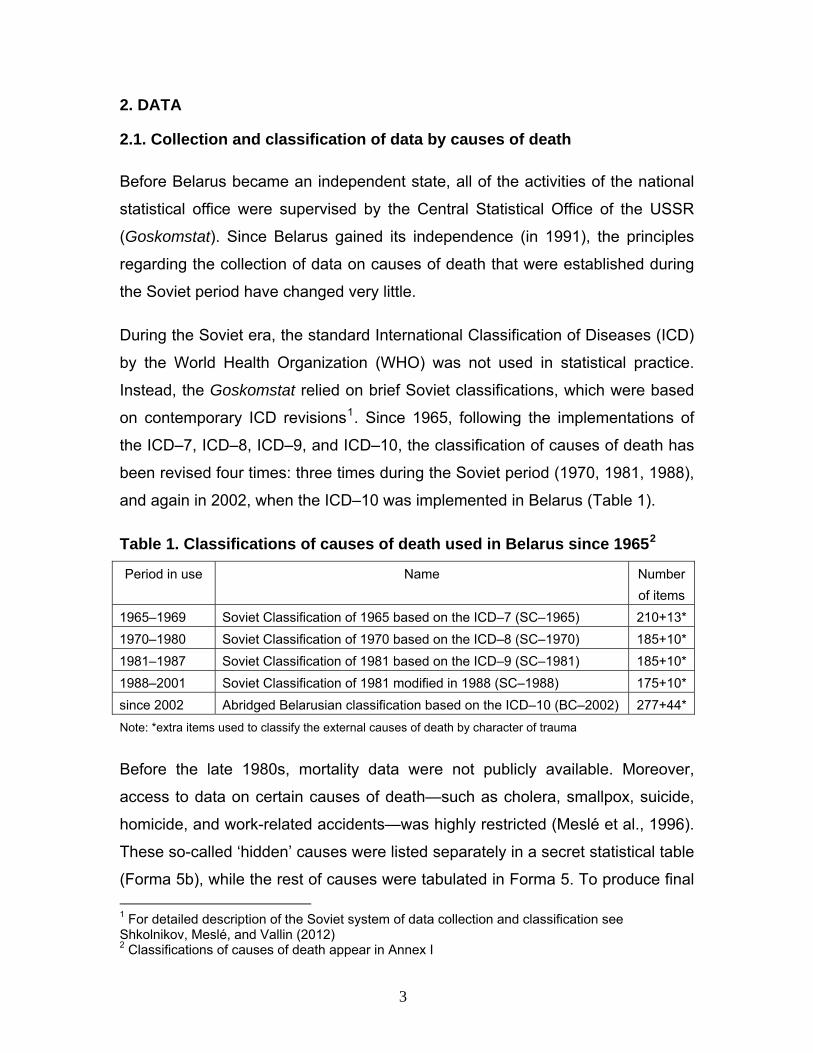
2. DATA

2.1. Collection and classification of data by causes of death

Before Belarus became an independent state, all of the activities of the national

statistical office were supervised by the Central Statistical Office of the USSR

(Goskomstat). Since Belarus gained its independence (in 1991), the principles

regarding the collection of data on causes of death that were established during

the Soviet period have changed very little.

During the Soviet era, the standard International Classification of Diseases (ICD)

by the World Health Organization (WHO) was not used in statistical practice.

Instead, the Goskomstat relied on brief Soviet classifications, which were based

on contemporary ICD revisions1. Since 1965, following the implementations of

the ICD–7, ICD–8, ICD–9, and ICD–10, the classification of causes of death has

been revised four times: three times during the Soviet period (1970, 1981, 1988),

and again in 2002, when the ICD–10 was implemented in Belarus (Table 1).

Table 1. Classifications of causes of death used in Belarus since 19652

Period in use Name Number of items

1965–1969 Soviet Classification of 1965 based on the ICD–7 (SC–1965) 210+13* 1970–1980 Soviet Classification of 1970 based on the ICD–8 (SC–1970) 185+10* 1981–1987 Soviet Classification of 1981 based on the ICD–9 (SC–1981) 185+10* 1988–2001 Soviet Classification of 1981 modified in 1988 (SC–1988) 175+10* since 2002 Abridged Belarusian classification based on the ICD–10 (BC–2002) 277+44* Note: *extra items used to classify the external causes of death by character of trauma

Before the late 1980s, mortality data were not publicly available. Moreover,

access to data on certain causes of death—such as cholera, smallpox, suicide,

homicide, and work-related accidents—was highly restricted (Meslé et al., 1996).

These so-called ‘hidden’ causes were listed separately in a secret statistical table

(Forma 5b), while the rest of causes were tabulated in Forma 5. To produce final 1 For detailed description of the Soviet system of data collection and classification see Shkolnikov, Meslé, and Vallin (2012) 2 Classifications of causes of death appear in Annex I

3

statistical tables by causes of death, the total number of deaths from Forma 5b

was added to the number from Forma 5. To ensure that the sum of all the items

in Forma 5 yielded the total, all of the ‘hidden’ causes were assigned to ill-defined

causes. In 1988, Gorbachev’s new policy of glasnost resulted in the release of

mortality statistics, and the notion of ‘hidden’ causes was abolished. Since then,

the cause-of-death data for Belarus have been produced in the format of the

electronic statistical Table C51. Over the entire period since 1965, cause-specific

mortality data have been reported using the same age grouping scale: 0, 0-27

days, 1, 2, 3, 4, 5-9, 10-14,…, unknown age, 85+, all ages combined.

2.2. Collected data

The collection, verification, and systematic arrangement of cause-specific

mortality data proved to be time-consuming tasks. Fortunately, the Belarusian

data of the Soviet period (1965–1990) were readily available to us in

computerized format, thanks to the work done by a joint project of the Russian

Center for Demography and Human Ecology and the French National Institute for

Demographic Studies. Within the framework of this project, which was launched

in 1990, cause-specific mortality data were gathered from archives and

computerized for all 15 republics of the former USSR (Shkolnikov, Meslé, Vallin,

1997). For the post-Soviet period (except 1991–1996), data were obtained

directly from the National Statistical Committee of Belarus (Belstat). The final

pieces of the data (1991–1996) were obtained in a computerized format from the

WHO Office for Europe.

2.3. Data consistency checks

We began our work by preparing and arranging the data. At this stage, it was

particularly important to ensure that the data were entered correctly, and they

were both internally and externally consistent. First, we performed a number of

checks, including, for example, of whether the death counts by age groups were

in line with the totals, and of whether the input data contained duplicated records.

Next, we compared our raw data (all causes combined) with the death counts

4

from the Human Mortality Database (HMD)1. The data available at the HMD

originated from the statistical table Forma 4 (now Table 42), “Distribution of

deaths by single year of age and sex.” In theory, there should be no differences

between two datasets: the total numbers of death from all causes of death in

Forma 5 (now Table C51) should be exactly equal to the death counts in the

HMD by each age group. In fact, there were some deviations, which were

corrected accordingly. Finally, after checking the data, we redistributed the

deaths of unknown age proportionally among the other age groups.

2.4. Data quality

Problems related to the quality of mortality statistics in Belarus were much more

significant in the past (the 1960s-1970s) than they have been in more recent

years. It is widely recognized that mortality data in the former Soviet Union

suffered from various kinds of measurement errors, such as the under-

registration of infant mortality, age heaping, and age exaggeration at old ages

(Anderson and Silver, 1986, 1997; Blum and Monnier 1989; Grigoriev 2007). One

of the most notable inconsistencies, which led to the distortion of overall mortality

statistics, was related to the reporting of infant deaths. For this reason, prior to

the reconstruction of mortality trends, we performed a correction of the infant

deaths (see Section 3). This adjustment was also necessary to ensure that the

statistics remained comparable with those of the other former Soviet republics,

for which reconstructed mortality trends were also adjusted for the under-

counting of infant deaths.

Many factors, such diagnostics, coding, and the specific characteristics of

medical schools (which also evolve over time), can affect the quality of cause-

specific mortality data. One of the most reliable ways to assess the quality of

mortality data is to conduct special surveys that examine the validity of diagnoses

in the medical death certificates. One such survey was conducted in the

Belarusian capital of Minsk in 1981-1982. Using a sample of medical death

certificates, qualified physicians checked both the validity of diagnoses and the 1www.mortality.org

5

correctness of their coding. According to the results of this survey, the overall

proportion of erroneous diagnoses constituted 6.6 per cent. The highest share

(23.2 per cent) of errors was observed in the diagnosis of infectious diseases,

followed by in the diagnosis of digestive (12.8 per cent) and respiratory (11.8 per

cent) diseases. In coding, most errors occurred while coding deaths from

diseases of the genitourinary system (11.8 per cent). For the remaining causes,

the share of errors did not exceed eight per cent. Since in many cases errors in

diagnostics and coding balanced each other out, the percentages of errors that

were finally reflected in the statistics turned to be quite acceptable at the level of

broad groups of causes (Shkolnikov, Meslé, Vallin, 2012).

To our knowledge, no surveys similar to one conducted in Minsk were

undertaken in post-Soviet Belarus. Generally, evidence regarding the validity and

reliability of recent mortality data for Belarus is scarce. It has been suggested

that the mortality data in the countries of the European part of the former USSR

are trustworthy. Anderson and Silver (1997) noted that the recent mortality data

in these countries “are generally reliable, especially at the working ages.” On the

basis of data quality indicators—such as timeliness, completeness, coverage of

death registration, and the proportion of deaths assigned to ill-defined causes

during the period 1981-2001—the WHO has assigned Belarus to the category of

countries with mortality data of medium quality (Mathers et al. 2005).

6

3. Correction for under-reported infant deaths

Before the 1970s, the infant death records in the USSR were incomplete. In 1974, with the introduction of a new certificate of perinatal death, the registration of infant mortality improved, and the infant mortality rate therefore increased1 (Anderson and Silver 1986). Yet a considerable share of the infant deaths remained unreported because of the use in Soviet statistical practices of a specific definition of live birth that was not in line with the standard WHO definition. According to the Soviet definition, infants born before 28 weeks of gestation who weighed less than 1,000 grams or who measured less than 35 centimeters in length were not counted as either live births or infant deaths, if they died before completing the first seven days of life.

The Soviet definition of live birth was in force in Belarus until 1994, when the transition to the WHO definition was officially announced. The adoption of the international standards of live and stillbirths was expected to lead to a considerable increase in early neonatal mortality, and thus in neonatal and infant mortality. For example, the implementation of the WHO definition in the Baltic countries resulted in a 50 per cent increase in early neonatal mortality (Estonian Medical Statistics Bureau, Latvian Medical Statistics Bureau, Lithuanian Medical Statistics Bureau, 1993). By contrast, our estimates based on official data indicate that the increase in early neonatal mortality in Belarus after the declared shift to the WHO definition constituted only 20 per cent. This suggests that the announced transition to the standard WHO definition was only partially implemented in Belarus.

According to the WHO definition, a newborn who breathes or shows any sign of life is counted as a live birth, regardless of the length of gestation. Yet the ‘new’ definition of live birth in Belarus imposes an additional requirement that the birth weight is greater than 500 grams, the body length is 25 cm or more, and the duration of gestation is at least 22 weeks. Thus, even the new definition does not conform to the WHO criteria. Moreover, after the announcement of the transition to the WHO definition, the statistical office of Belarus developed a system that

1 Some scholars argued that deteriorating infant mortality trends were real and attributable to the poor performance of the Soviet health care system (Davis and Feshbach 1980)

7

calculated infant mortality according to ‘old’ and ‘new’ criteria of viability. During 1994-2000, the infant mortality rate was, under the new definition, 8.8% to 12.9% higher than the rate based on the old criteria (Shakhotko 2003). It appears that, for a number of years after the new definition of live birth was adopted, the officially published infant mortality rates were calculated on the basis of the old Soviet definition of live birth.

However, an increase in neonatal mortality in 1994 suggests that there were indeed some changes in the registration of live births. One decade later, in 2005, there was again a noticeable increase in neonatal mortality in Belarus (Figure 1). It is likely that this undocumented change occurred not because of the change in the definition of live birth and in its practical interpretation, but simply because infant mortality rates were calculated on the basis of the new criteria for viability, which had finally been released for publication.

Figure 1. Neonatal and infant mortality rates in Belarus; both sexes, 1965-2010

8

Given the problems mentioned above, we considered it reasonable to correct the

data on infant deaths. Since the problems with the registration of infant mortality

were primarily related to the registration of deaths during the first days of life,

neonatal mortality rates were corrected first. On the basis of the adjusted

neonatal mortality rates, we calculated the under-counted neonatal deaths,

keeping in mind that these extra deaths should have also counted as live births.

Subsequently, the nominator and denominator of the infant mortality rates were

adjusted for missing deaths and live births, respectively. The correction was

accomplished in three steps. Figure 2 shows the results of these corrections.

Figure 2. Corrections of neonatal mortality and their effects on infant mortality in Belarus; both sexes, 1965-2010

9

First, we corrected neonatal mortality rates during 1965-1973. We applied the

correction factor1 of 20 per cent to account for the under-registration of neonatal

deaths during this period. Second, neonatal mortality trends during 1965-1993

were adjusted while taking into account the change that occurred in 1994. As

was mentioned above, no real transition to the standard WHO definition

happened at this point, but some changes regarding the definition of live birth did

indeed occur. To account for them, we applied the correction factor of 10 per

cent. This resulted in a further increase in the IMR. Finally, neonatal mortality

trends over 1965-2004 were adjusted using the correction factor of 25 per cent.

In the next step, we needed to make the adjusted IMR consistent with the data

on causes of death. To bring these figures into line, we first performed a

redistribution of the extra deaths among causes of death within the age group 0-

27 days. The numbers by each cause of death were then added to deaths at age

zero, and to the total number of deaths. All of these manipulations were

performed separately by sex. Population exposure was adjusted accordingly for

under-counted live births.

The adjustments for the under-counting of infant deaths and live births had

significant effects on the neonatal and infant mortality trends. But to what extent

did the adjusted IMR affect the dynamics of life expectancy at birth? To answer

this question, we computed life tables before and after the correction of the IMR

for each year since 1965. As expected, the correction of infant mortality did not

have a very significant impact on life expectancy trends in Belarus (Table 2). The

difference between the initial and the adjusted life expectancy throughout the

entire period did not exceed 0.3 years.

1 Applied correction factors are arbitrary values based on the assumption that neonatal mortality rates in the two successive years (before and after the change) remain at nearly the same level

10

Table 2. Life expectancy at birth in Belarus before and the correction of infant mortality by sex, 1965–2004 (in years)

Males Females Year

Before After Difference Before After Difference

1965 68.96 68.64 -0.32 76.14 75.86 -0.28

1970 67.86 67.53 -0.33 75.95 75.65 -0.31

1975 67.15 66.94 -0.21 76.25 76.08 -0.17

1980 65.94 65.69 -0.25 76.20 76.01 -0.19

1985 67.70 67.46 -0.24 76.29 76.12 -0.18

1990 65.52 65.31 -0.21 75.47 75.31 -0.16

1995 63.04 62.90 -0.14 74.30 74.19 -0.11

2000 62.75 62.67 -0.08 74.52 74.46 -0.06

2004* 63.17 63.11 -0.06 75.00 74.95 -0.05

*no correction after 2004

4. Method of reconstruction

How to bridge the gaps between the old and the new sets of causes of deaths is

the central problem to be solved. As the first step, the method assumes the

construction of two correspondence tables. The goal is to provide a systematic

comparison of the medical content between two successive revisions of causes

of death. The correspondence tables consist of two reciprocal directories. One

directory assigns to each item of the new classification all of the items of the old

classification that they share, or at least a portion of its medical content. In the

second directory, all of the mutual correspondences are listed again but sorted

by items of the old revision (Pechholdova, 2009). The correspondence tables

serve as the basis for building fundamental associations (FA), or the smallest

possible clusters of causes of death sharing the same medical content within two

successive revisions1. Depending on the complexity of the exchanges between

the items, four types of association could be defined. The simplest type, 1:1,

assumes a simple (one-to-one) correspondence between one item from the old

and one item from the new revision. Type (1:N) assumes that one item from the

1 Meslé and Vallin (1996) and Pechholdova (2009) provide detailed explanations on this point.

11

old revision corresponds to N (more than one) items in the new revision. Type

(N:1) refers to associations in which N items of the old revision correspond to one

item in the new revision. And, finally, type (N:N) assumes the complex exchange

between several items from the old revision and several items from the new

revision.

These fundamental associations allow us to estimate transition coefficients: i.e.,

positive values between zero and one that explicitly determine the mathematical

correspondence between items of the old and the new revisions. Finally,

transition coefficients are applied to the death counts of the old revision that are

to be transformed into respective items of the new revision. In the end, the

coherent time series of the new classification are obtained. During the

reconstruction work for Belarus, the procedure was refined by implementing the

concept of the so-called ‘transition matrix’. The transition matrix (TM) is a

summary table containing all of the transition coefficients, and therefore showing

the correspondence between all of the items in the old and the new revisions

simultaneously. After the transition matrix has been filled with transition

coefficients, the cause-specific ‘new’ death counts can be obtained by using the

following matrix equation:

D’=TM·D (1)

where D’ and D are the matrices of the new and the old death counts. The

explicit expression of the product is:

⎥⎥⎥⎥

⎦

⎤

⎢⎢⎢⎢

⎣

⎡

×

⎥⎥⎥⎥

⎦

⎤

⎢⎢⎢⎢

⎣

⎡

=

⎥⎥⎥⎥

⎦

⎤

⎢⎢⎢⎢

⎣

⎡

′′′

′′′′′′

mxmm

x

x

nmnn

m

m

nxnn

x

x

ddd

dddddd

tmtmtm

tmtmtmtmtmtm

ddd

dddddd

L

MOMM

L

L

L

MOMM

L

L

L

MOMM

L

L

21

22221

11211

21

22221

11211

21

22221

11211

(2)

where n and m is the number of items in the new and the old classifications,

respectively, and x is the number of age groups. Thus, the value of an element

tm12, for example, indicates the proportion of item 2 in the new revision to be

redistributed into item 1 of the old revision. Clearly, if an element tm is equal to

12

zero (which is in fact the case with most of the TM elements), then there is no

exchange between the respective items. Element d12 represents the number of

deaths from cause 1 in age group 2 of the old revision, while element d’12 refers

to the number of deaths in same age group, but this time classified as cause 1 in

accordance with the new revision.

Sometimes there is a need to reclassify death counts in accordance with the old

revision. In such cases, the same logic is applied, but the TM should be filled with

different transition coefficients. This time, the rows and columns of the TM will

refer to the number of items in the old and new classifications, respectively; and

an element tm will indicate the share of the item of the new revision to be

assigned to the item of the old revision.

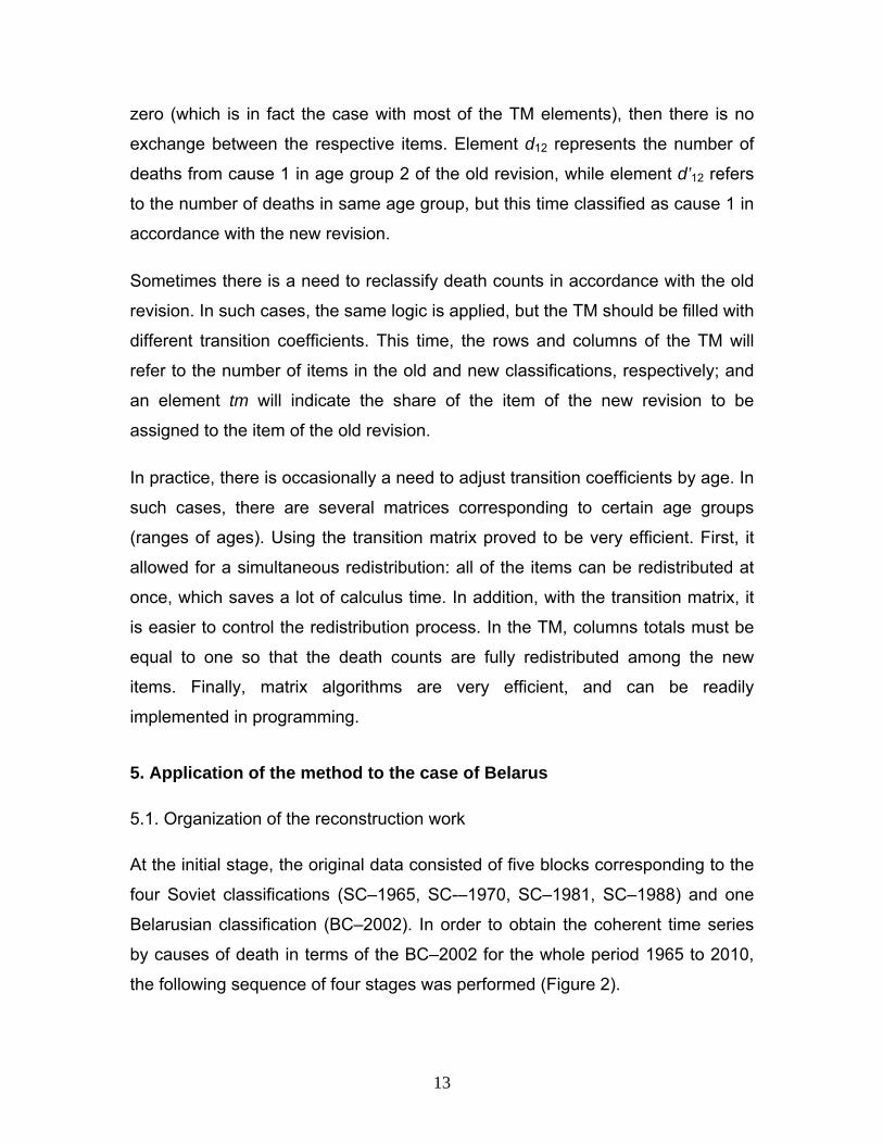
In practice, there is occasionally a need to adjust transition coefficients by age. In

such cases, there are several matrices corresponding to certain age groups

(ranges of ages). Using the transition matrix proved to be very efficient. First, it

allowed for a simultaneous redistribution: all of the items can be redistributed at

once, which saves a lot of calculus time. In addition, with the transition matrix, it

is easier to control the redistribution process. In the TM, columns totals must be

equal to one so that the death counts are fully redistributed among the new

items. Finally, matrix algorithms are very efficient, and can be readily

implemented in programming.

5. Application of the method to the case of Belarus

5.1. Organization of the reconstruction work

At the initial stage, the original data consisted of five blocks corresponding to the

four Soviet classifications (SC–1965, SC-–1970, SC–1981, SC–1988) and one

Belarusian classification (BC–2002). In order to obtain the coherent time series

by causes of death in terms of the BC–2002 for the whole period 1965 to 2010,

the following sequence of four stages was performed (Figure 2).

13

Initial stage SC–1965 1965–1969

(n=210)

SC–1970 1970–1980

(n=185)

SC–1981 1981–1987

(n=185)

SC–1988 1988–2001

(n=175)

BC–2002 2002–2010

(n=277)

Stage I 1965-1980 (n=185)

Stage II 1965-1987 (n=185)

Stage III 1965-2001 (n=175)

Stage IV 1965-2010 (n=277)

Figure 3. Four Major Stages of Reconstruction Note: n is number of items in the cause-of-death classification

The first stage of the reconstruction permitted us to overcome the transition from

the SC–1965 to the SC–1970, and to obtain coherent time series for 1965-1980

in terms of the SC–1970. The next stage included the reconstruction of cause-

specific mortality trends in terms of the SC–1981 for the period 1965-1987. The

third stage aimed at reconstructing cause-specific mortality trends in terms of the

SC–1988 for the period 1965–2001. Finally, we reconstructed continuous series

for the whole period of 1965 to 2010 in terms of the BC–2002.

5.2. Transition to the SC–1970: a detailed example

As it is impossible to provide all of the details of the laborious reconstruction

procedure, we will demonstrate only its principal steps by focusing on the

transition that occurred in 1970. Here, we will show how we reclassified the items

of the SC–1965 as items of the SC–1970. The main steps of the procedure

(defining the fundamental associations of items and estimating the transition

coefficients) will be accompanied by detailed examples. We will then briefly

address the main methodological issues related to the other transitions (SC–

1981, SC–1988, and BC–2002).

Fundamental associations

The first step of the reconstruction was to overcome the transition that occurred

in 1970. Formally, we were supposed to begin the reconstruction from the

14

construction of correspondence tables. Fortunately, we could skip this step and

rely on the results of similar work previously conducted for Russia (Meslé et al.,

1996). Theoretically, Belarus and Russia, belonged to a single system of data

collection and classification, and were supposed to follow the same coding rules

and instructions. Thus, the transition coefficients obtained for one country should

have been applicable to the other.

This was found to be only partially the case after we examined the time series by

each cause of death and applied the Russian TC. In some cases, the transition

coefficients fitted well, while in others they did not. In some cases, the precision

of the Russian TC (estimated for a much larger population) was not justified,

especially when the TC varied across ages. Taking all of these limitations into

account, we decided to start the work by rebuilding the FA. First, we filled the

existing Russian FA with the death counts for two successive years (1969 and

1970). We then visually inspected the statistical balance for each FA (Figure 4).

The strategy at this stage was to identify and then modify all of the ‘unbalanced’

FA (i.e., those exhibiting notable ruptures between the trends before and after

the transition year). After several rounds of inspections and modifications, the FA

were established.

15

Figure 3. Four types of fundamental associations and the initial (unreconstructed) items included in them Note: The labels on the left-hand side of the graphs (before year 1970) are numbers of items in the SC–

1965, while the labels on the right-hand side are numbers of items in the SC–1970. Their names are

provided below in the text.

Transition coefficients

Once the FA were determined, we could proceed to the estimation of the TC.

Obviously, in the case of a simple association, there is only one transition

coefficient equal to one. Thus, in association 49, item 59 of the SC–1965,

“Malignant neoplasm of the breast,” was reclassified as item 57 of the SC–1970.

16

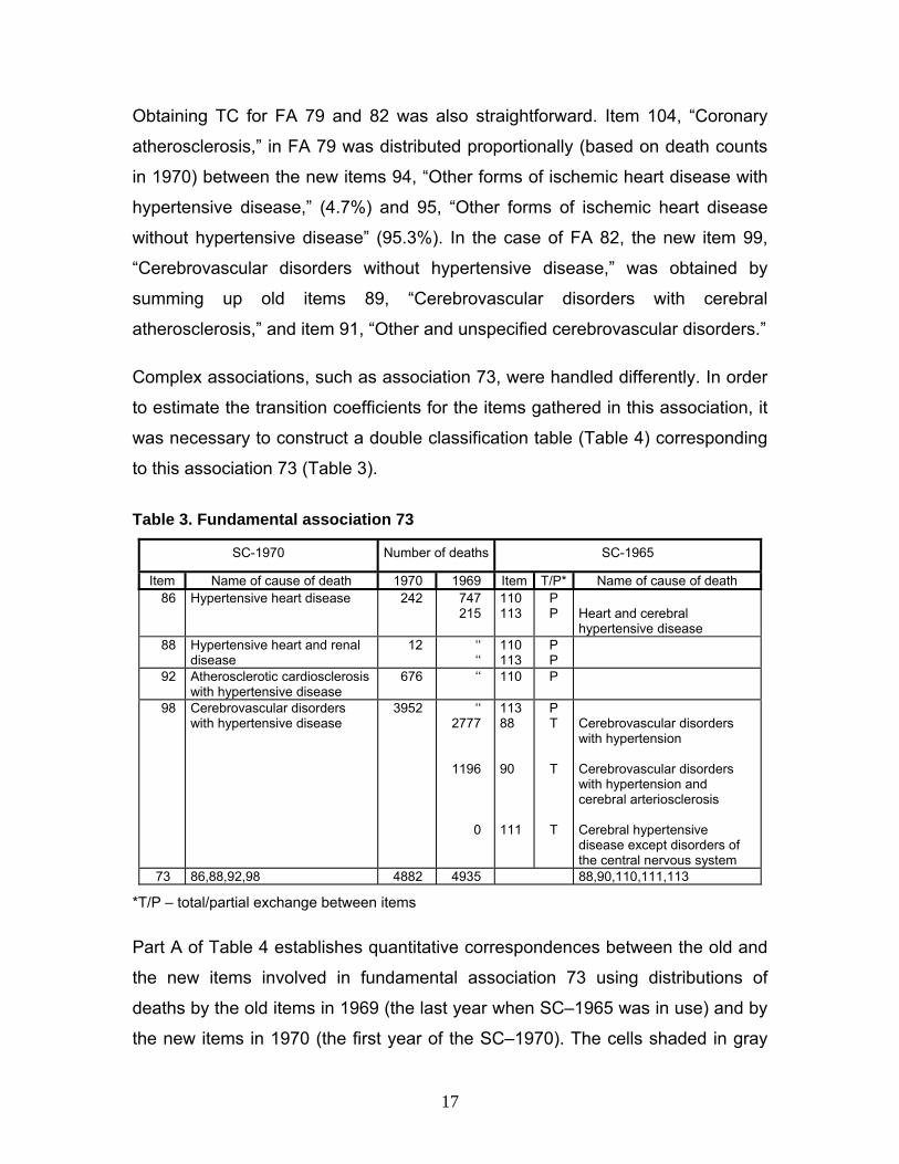
Obtaining TC for FA 79 and 82 was also straightforward. Item 104, “Coronary

atherosclerosis,” in FA 79 was distributed proportionally (based on death counts

in 1970) between the new items 94, “Other forms of ischemic heart disease with

hypertensive disease,” (4.7%) and 95, “Other forms of ischemic heart disease

without hypertensive disease” (95.3%). In the case of FA 82, the new item 99,

“Cerebrovascular disorders without hypertensive disease,” was obtained by

summing up old items 89, “Cerebrovascular disorders with cerebral

atherosclerosis,” and item 91, “Other and unspecified cerebrovascular disorders.”

Complex associations, such as association 73, were handled differently. In order

to estimate the transition coefficients for the items gathered in this association, it

was necessary to construct a double classification table (Table 4) corresponding

to this association 73 (Table 3).

Table 3. Fundamental association 73

SC-1970 Number of deaths SC-1965

Item Name of cause of death 1970 1969 Item T/P* Name of cause of death 86 Hypertensive heart disease 242 747

215 110113

P P

Heart and cerebral hypertensive disease

88 Hypertensive heart and renal disease

12 ‘‘‘‘

110113

P P

92 Atherosclerotic cardiosclerosis with hypertensive disease

676 ‘‘ 110 P

98 Cerebrovascular disorders with hypertensive disease

3952

‘‘2777

1196

0

11388 90 111

P T

T

T

Cerebrovascular disorders with hypertension Cerebrovascular disorders with hypertension and cerebral arteriosclerosis Cerebral hypertensive disease except disorders of the central nervous system

73 86,88,92,98 4882 4935 88,90,110,111,113

*T/P – total/partial exchange between items

Part A of Table 4 establishes quantitative correspondences between the old and

the new items involved in fundamental association 73 using distributions of

deaths by the old items in 1969 (the last year when SC–1965 was in use) and by

the new items in 1970 (the first year of the SC–1970). The cells shaded in gray

17

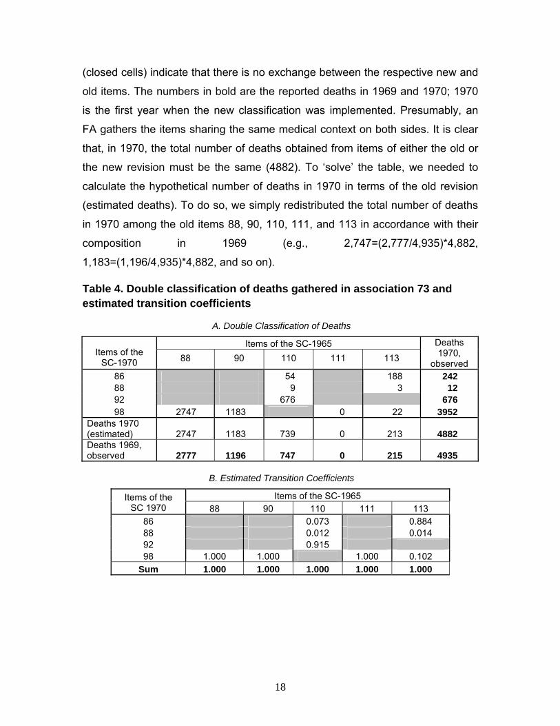
(closed cells) indicate that there is no exchange between the respective new and

old items. The numbers in bold are the reported deaths in 1969 and 1970; 1970

is the first year when the new classification was implemented. Presumably, an

FA gathers the items sharing the same medical context on both sides. It is clear

that, in 1970, the total number of deaths obtained from items of either the old or

the new revision must be the same (4882). To ‘solve’ the table, we needed to

calculate the hypothetical number of deaths in 1970 in terms of the old revision

(estimated deaths). To do so, we simply redistributed the total number of deaths

in 1970 among the old items 88, 90, 110, 111, and 113 in accordance with their

composition in 1969 (e.g., 2,747=(2,777/4,935)*4,882,

1,183=(1,196/4,935)*4,882, and so on).

Table 4. Double classification of deaths gathered in association 73 and estimated transition coefficients

A. Double Classification of Deaths

Items of the SC-1965 Items of the

SC-1970 88 90 110 111 113

Deaths 1970,

observed 86 54 188 242 88 9 3 12 92 676 676 98 2747 1183 0 22 3952

Deaths 1970 (estimated) 2747 1183 739 0 213 4882 Deaths 1969, observed 2777 1196 747 0 215 4935

B. Estimated Transition Coefficients

Items of the SC-1965 Items of the SC 1970 88 90 110 111 113

86 0.073 0.884 88 0.012 0.014 92 0.915 98 1.000 1.000 1.000 0.102

Sum 1.000 1.000 1.000 1.000 1.000

18

The next step was to redistribute deaths among the non-shaded cells of the table

so that the column and row totals equaled the known marginal totals shown in

bold. To accomplish this, we first filled in the cells corresponding to a 100-per

cent exchange between the old and the new items. All of the 2,747 deaths of old

item 88 were distributed into new item 98.

The same logic applied to old items 90 and 111, for which all deaths had to be

transferred to new item 98. New item 92 took 676 deaths from old item 110. We

could then see that the number of deaths corresponding to items 98 and 113

must have been equal to 22 (22=3,952-2,747-1,183-0). After this was done, there

was not a unique solution for the redistribution of deaths among the remaining

cells. This could have been applied in several different ways. In this particular

case, we assumed that the total number of 12 deaths in new item 88 could be

distributed between old items 110 and 113 according to their shares in 1969

(78=747/(747+215)*100 and 22=215/(747+215)*100 per cent, respectively.

Consequently, new item 88 received nine deaths (78 per cent) from old item 110,

and three deaths (22 per cent) from old item 113. Finally, the remaining non-

shaded cells were filled in by subtraction. Once the deaths had been

redistributed and the totals were verified, we could obtain the transition

coefficients (Part B of Table 4). These TC were linked to the transition matrix in

such a way that they could be filled in and updated automatically. Table 5 depicts

a fragment of the transition matrix filled with the transition coefficients estimated

from the association. The items of the SC-1965 (from one to 210) appear in

columns (from left to right), and the items of the SC-1970 (from one to 185)

appear in rows (from top to bottom). The sum of the transition coefficients always

had to be equal to one to ensure that no deaths ‘got lost’ during the transition to a

new classification.

Applying equation (1) allowed us to estimate the new death counts for all causes

simultaneously. Figure 4 depicts the results, including the trends by each cause

of death involved in association 73 before and after the reconstruction.

19

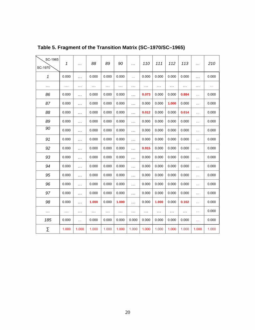
Table 5. Fragment of the Transition Matrix (SC–1970/SC–1965)

SC-1965

SC-1970 1 … 88 89 90 … 110 111 112 113 … 210

1 0.000 … 0.000 0.000 0.000 … 0.000 0.000 0.000 0.000 … 0.000

… … … … … … … … … … … … …

86 0.000 … 0.000 0.000 0.000 … 0.073 0.000 0.000 0.884 … 0.000

87 0.000 … 0.000 0.000 0.000 … 0.000 0.000 1.000 0.000 … 0.000

88 0.000 … 0.000 0.000 0.000 … 0.012 0.000 0.000 0.014 … 0.000

89 0.000 … 0.000 0.000 0.000 … 0.000 0.000 0.000 0.000 … 0.000

90 0.000 … 0.000 0.000 0.000 … 0.000 0.000 0.000 0.000 … 0.000

91 0.000 … 0.000 0.000 0.000 … 0.000 0.000 0.000 0.000 … 0.000

92 0.000 … 0.000 0.000 0.000 … 0.915 0.000 0.000 0.000 … 0.000

93 0.000 … 0.000 0.000 0.000 … 0.000 0.000 0.000 0.000 … 0.000

94 0.000 … 0.000 0.000 0.000 … 0.000 0.000 0.000 0.000 … 0.000

95 0.000 … 0.000 0.000 0.000 … 0.000 0.000 0.000 0.000 … 0.000

96 0.000 … 0.000 0.000 0.000 … 0.000 0.000 0.000 0.000 … 0.000

97 0.000 … 0.000 0.000 0.000 … 0.000 0.000 0.000 0.000 … 0.000

98 0.000 … 1.000 0.000 1.000 … 0.000 1.000 0.000 0.102 … 0.000

… … … … … … … … … … … … 0.000

185 0.000 … 0.000 0.000 0.000 0.000 0.000 0.000 0.000 0.000 … 0.000

∑ 1.000 1.000 1.000 1.000 1.000 1.000 1.000 1.000 1.000 1.000 1.000 1.000

20

Items of SC 1965 Items of SC 1970

88 Cerebrovascular disorders with hypertension

86 Hypertensive heart disease

90 Cerebrovascular disorders with hypertension and cerebral arteriosclerosis

88 Hypertensive heart and renal disease

110 Hypertensive heart disease except myocardial infarction

92 Atherosclerotic cardiosclerosis with hypertensive disease

111 Cerebral hypertensive disease except disorders of the central nervous system

98 Cerebrovascular disorders with hypertensive disease

113 Heart and cerebral hypertensive disease

Figure 4. Trends in deaths by causes of death involved in association 73 before and after the reconstruction

21

5.3. Other transitions

Applying the described procedures, we overcame incrementally the three

remaining transitions of 1981, 1988, and 2002. In the following, we will briefly

highlight the main issues related to these transitions.

Soviet Classification of 1981 (SC–1981)

The transition to the SC–1981 was conducted in the same manner as the

previous one. As in the case of the transition to the SC–1970, the direct

application of the Russian TC on Belarusian data was not enough to eliminate

discontinuities in trends produced by the implementation of the new classification

in 1981. Once again, the best strategy was to use the earlier experience, and to

rely on the Russian FA at the initial stage. Thus, we first filled the Russian FA

with Belarusian death counts. We then checked the statistical balance for each

association, re-built the FA when necessary, and compiled the final list of FA to

be used for estimating the TC. After applying the newly estimated TC, we

extended the series up to 1987.

Soviet Classification of 1988 (SC-1988)

The next step was to bridge 185 reconstructed items (1965-1987) with 175 items

of the SC–1988 , and extend the series until 2001. In 1988, the notion of ‘hidden’

causes of death was abolished. It was also decided that work-related accidents

would no longer be classified as separate items. For example, deaths from

accidental falls had previously been assigned to two separate items: “accidental

falls” and “work-related accidental falls.” After the change, all deaths from

accidental falls were assigned to just one item, “accidental falls.” As a result,

items 160 to 185 in the SC–1981 were transformed into items 160 to 175. Since

the first 159 items in the modified classification remained unchanged, and the

correspondences between the remaining items were simple, dealing with the

changes introduced in 1988 was not problematic.

22

Belarusian abridged version of the ICD–10 (BC–2002)

There are two principal differences between the classification changes

implemented during the Soviet era and the transition to the ICD–10. First, unlike

in the case of this transition, the earlier classification changes were outlined and

implemented in Belarus under the centralized supervision of the Goskomstat.

The role of the local statistical authorities was simply to ensure the proper

execution of the process. Second, and more importantly, the implementation of

the ICD–10 produced many more changes than the previous revisions. The

complexity of the ICD–10, the lack of experience of the governmental bodies

responsible for the process, and the financial constraints of the transition period

might explain why the ICD–10 implementation in Belarus occurred relatively late,

in 2002. Unlike for the previous transitions, we could not rely upon the Russian

experience. Instead, we used the official document released by the Ministry of

Statistics and Analysis of Belarus in 2004 as the starting point for our work. This

document contains the items of the so-called “abridged nomenclature” based on

the ICD–10, their correspondences to the full list of the ICD–10 items, as well as

the theoretical correspondences to the items of the previous nomenclature (SC–

1988).

The existence of the theoretical associations between items was very helpful. But

after filling in the death counts in these associations and checking the statistical

balance, we found that many of the associations seemed implausible, and thus

required modifications. After several rounds of adjustments, we were finally able

to compile the ultimate list of associations. Then, by following the sequence of

standard steps, we overcame the last transition, and extended the harmonized

series up to 2010.

We encountered much more complex problems during the last transition than in

the previous transitions. These problems were not only related to the transition

year, but also to the period thereafter. One of them was the diagnosis of

cardiovascular diseases (CVD) with the distinction of conditions either involving

23

or not involving hypertensive heart disease (HHD). Unlike the original ICD-10, the

special abridged version of the ICD-10 currently used in Belarus makes this

distinction. The dynamics of the reconstructed trends indicated an almost

symmetrical exchange between items with and without HHD after the transition in

2002 (Figure 5).

It appeared that there were significant changes in the diagnosis of cardiovascular

mortality, as growing numbers of deaths from CVD were diagnosed as involving

HHD. Clearly, in this case, breaks in the time series could not be eliminated

through a reconsideration of the associations between items. To overcome the

problem, other solutions had to be considered. Aggregating items into bigger

groups (e.g., ischemic heart diseases, cerebrovascular diseases) appeared to be

an appropriate solution, as it allowed us to avoid making the distinction between

problematic hypertensive and non-hypertensive CVD deaths.

24

Figure 5. Trends by selected causes of death after the transition to the BC-2002; both sexes, 1965-2010 Notes:

134 “Atherosclerotic cardiosclerosis with HHD”

135 “Atherosclerotic cardiosclerosis without HHD”

136 “Other forms of chronic ischemic heart disease with HHD”

137 “Other forms of chronic ischemic heart disease without HHD”

148 “Cerebral infarction with HHD”

149 “Cerebral infarction without HHD”

152 “Other cerebrovascular disorders with HHD”

153 “Other cerebrovascular disorders without HHD”

25

5.4. Beyond classification change: a posteriori corrections

Not all of the discontinuities observed in the reconstructed trends are related to

official classification changes. Independent of the transitions to new

classifications, changes in coding practices might occur at any time. In such

cases, the trends are subject to so-called a posteriori corrections.

Let us recall the reconstructed trends of association 73 (see Figure 4). The

trends show no ruptures around the transition year. However, in 1966, there was

an unusually large increase in the number of deaths in item 98 which was not

related to the transition to the SC–1970. Presumably, in 1965, some share of the

deaths belonging to item 98, “Cerebrovascular disorders with hypertensive

disease,” were mistakenly classified as item 99, “Cerebrovascular disorders

without hypertensive disease.” A closer examination of the trends of both items

revealed that the exchange between the two items occurred due to incorrect

registration at old ages. Figure 6 shows the results of an a posteriori correction,

applied in this case to ages 75 and above.

26

Figure 6. A posteriori corrections of items 98 and 99; 1965, both sexes, ages 75+, 20 per cent

Notes:

Item 98, “Cerebrovascular disorders with hypertensive disease”

Item 99, “Cerebrovascular disorders without hypertensive disease”

For this correction, we assumed that 20 per cent of the deaths assigned to item

99 should be reclassified into item 99. Figure 7 shows the effect of the correction

at ages 75, and on the mortality trends from all ages combined.

27

Figure 7. Results of a posteriori corrections of Items 98 and 99

Notes:

Item 98, “Cerebrovascular disorders with hypertensive disease”

Item 99, “Cerebrovascular disorders without hypertensive disease”

Another source of the discontinuities observed in the reconstructed trends could

be the changes in coding practices after the transition to a new classification.

Figure 8 depicts an example of the severe discontinuity in the trends in the

numbers of deaths from “other congenital anomalies of the central nervous

system” (item 149) and from “other congenital anomalies of the circulatory

system” (item 151), which occurred in Belarus in 1974.

28

Figure 8. A posteriori correction items 149 and 151; 1965–1973, both sexes, ages 0–14, 75 per cent

The corrections shown are based on the reasonable assumption that, prior 1974,

deaths from “other congenital anomalies of central nervous system” were

classified as “other congenital anomalies of the circulatory system.”

The last example (Figure 9) shows how the erroneous exchange in 1981 of item

48, “Malignant neoplasms of small intestine,” with item 49, “Malignant neoplasms

of colon,” was corrected. Prior the transition, both of these items were classified

in the SC–1970 as item 49, “Malignant neoplasm of intestine including

duodenum.” It appears that in the transition year (1981), a large proportion of the

deaths belonging to item 49 were classified as item 48.

29

Figure 9. A posteriori correction of items 48 and 49, 1981, both sexes, ages 25+, 55 per cent

5.5. Redistribution of ill-defined causes

The final stage of our work was to deal with ill-defined causes of death. The

share of ill-defined causes of death in the total number of deaths varies not only

among countries, but also over time. In order to ensure the comparability of

mortality trends, a redistribution of the ill-defined causes of death had to be

considered. Under the assumption of independence, ill-defined causes can be

redistributed proportionally among the other causes. Alternatively, they can be

redistributed only among certain items that are believed to be related to ill-

defined deaths.

In 1989, the Ministry of Health of the USSR issued an order regarding the

registration of senility and diseases of the circulatory system among individuals

aged 80 and older. Under the new instructions, all cases of death after age 80

had to be classified as senility, with the exception of violent deaths and deaths

30

for which diagnoses were confirmed by autopsy or medical record. In addition, all

of the cases of death from acute cardiovascular conditions under age 80 had to

be confirmed by autopsy. Otherwise, they had to be classified as ill-defined

(Meslé et al., 1996). Figure 10 demonstrates the sudden rise of senility in Belarus

after the implementation of the new rule.

Figure 10. Deaths from senility and atherosclerotic cardiosclerosis; both sexes, 1965-2010

In 1988, senility was reported in just 0.07 per cent of the total number of deaths.

But in the years that followed, the share of deaths attributed to senility rose

dramatically: to two per cent 1989, to nine per cent in 1990, and to 12 per cent in

1991. Over the same period, the share of deaths from “atherosclerotic

cardiosclerosis without hypertensive heart disease” (item 135 in BC–2002)

underwent an almost symmetrical decrease. This decrease is implausible given

the fact that, in the early 1990s, overall mortality in Belarus was rising. Because

of these problems, and also because there were reasons to suspect an

exchange between senility and item 135 (Meslé and Vallin, 2003, Vallin et al.,

31

2005), we decided to combine these items. Figure 11 shows the results of this

correction. The other ill-defined causes were redistributed proportionally among

all of the causes.

Figure 11. Deaths from atherosclerotic cardiosclerosis (item 135) before and after aggregating this cause with senility, both sexes, 1965-2010

6. Conclusion As a result of our work, Belarusian mortality series by causes of death, classified

according to the Belarusian classification of 2002, for the period 1965-2010 are

now freely available. If you are interested in using the data, please refer to the

annex of this report. It contains brief technical documentation, as well as a

description of the structure of the data files produced.

Acknowledgments This work benefited from the joint ANR-DFG research grant, “European

Divergence and Convergence in Causes of Death.” The authors are very grateful

to Vladimir Shkolnikov for his active participation in the project, as well as for his

constructive comments and suggestions for this report.

32

REFERENCES

Anderson, B. and Silver, B. (1986). Infant mortality in the Soviet Union: regional differences and measurement issues. Population and Development Review, 12(4), pp.705-738.

Anderson, B. and Silver, B. (1997). Issues of data quality in assessing mortality trends and levels in the New Independent States. In J. L. Bobadilla, C. Costello & F. Mitchell (Eds.), Premature death in the New Independent States (pp.120-155). Washington, DC, USA: National Academy Press

Blum, A. and Monnier, A. (1989). Recent mortality trends in the USSR: new evidence, Population Studies, 43(2), pp.211-241.

Davis, C. and Feshbach, M. (1980). Rising Infant Mortality in the USSR in the 1970s. International Population Reports. Series P-95, No. 7. Washington, D.C.: U.S. Government Printing Office.

Estonian Medical Statistics Bureau, Latvian Medical Statistics Bureau, Lithuanian Medical Statistics Bureau (1993). Health in the Baltic Countries, 1st edition. Tallin, Riga, Vilnius.

Fihel A., Meslé F., Vallin J. (2010). Mortality by causes of death in Poland 1970-2007: preliminary findings. Third Human Mortality Database Symposium, Paris 17-19 June 2010, 21 slides.

Grigoriev, P. (2007). About mortality data for Belarus. Human Mortality Database: Background and Documentation. University of California, Berkeley and Max Planck Institute for Demographic Research. Available at: http://www.mortality.org

Hertrich, V. and Meslé, F. (1997). Mortality by cause in the Baltic countries since 1970: a method for reconstructing time series. Revue Baltique, 10, pp.145–164.

Mathers, CD et al. (2005). Counting the Dead and What They Died From: an Assessment of the Global Status of Cause of Death Data. Bulletin of the World Health Organization. Vol. 83, No. 3, pp. 171-177.

33

Meslé, F., Shkolnikov, V., Vallin, J.(1992). Mortality by cause in the USSR population in the 1970-1987: The reconstruction of time series. European Journal of Population, 8, pp. 281-308.

Meslé, F. and Vallin, J. (2003). Mortalite et causes de deces en Ukraine au XXe siecle: la crise sanitaire dans les pays de l'ex-URSS. Paris, Les Cahiers de l'INED, 152.

Meslé, F., Shkolnikov, V., Hertrich, V., Vallin, J. (1996). Recent trends in mortality by causes of death in Russia during 1965-1994 [In French and Russian], Paris-Moscow.

Meslé, F. and Vallin, J. (1996). Reconstructing long-term series of causes of death. Historical methods, 29 (2), pp.72-87.

Meslé, F. and Vallin, J. (2012). Reconstructing series of deaths by cause with constant definitions. In Mortality and Causes of death in 20th-Century Ukraine. Demographic Research Monographs: a series of the Max Planck Institute for Demographic Research. pp. 131-152.

Vallin, J. and Meslé, F. (1988). Les causes de décès en France de 1925 à 1978, Paris, INED, PUF, Travaux et Documents, Cahier 115, 608 p.

Vallin, J., Andreev, E., Meslé, F., Shkolnikov, V. (2005). Geographical diversity of cause of death patterns and trends in Russia. Demographic Research 12(13), pp. 323-380.

Pechholdova, M. (2009). Results and observations from the reconstruction of continuous time series of mortality by cause of death: Case of West Germany, 1968-1997. Demographic Research, 21 (18), pp. 535-568.

Pechholdova M. (2010). Four decades of cause-specific mortality in the Czech Republic, West Germany and France, Prague, Charles University, 184 p. + CD-ROM (PhD Thesis).

Pechholdová, M., Meslé, F., Vallin, J. (2011). Metoda rekonstrukce souvislých řad úmrtí dle příčin: výsledky aplikace na Českou republiku. [The reconstruction of continuous time series of mortality by cause of death: application to the Czech Republic]. Demografie, 2011, 53: pp. 5–18.

34

Penina, O., Meslé, F., Vallin, J., 2010, “What causes of are driving life expectancy in Moldova”, Paper presented at the European Population Conference, Vienna.

Shkolnikov, V., Meslé, F., Vallin, J. (2012). Data collection, data quality and the history of cause-of-death classification. In Mortality and Causes of death in 20th-Century Ukraine. Demographic Research Monographs: a series of the Max Planck Institute for Demographic Research. pp. 121-130.

Shkolnikov, V., Meslé, F., Vallin, J. (1997). Recent trends in life expectancy and causes of death in Russia, 1970-1993. In: Bobadilla, J. L., Costello, C. and Mitchell, F. (eds.), Premature death in the New Independent States, Washington, DC, National Academy Press, pp.34-65.

Shakhotko, L. (2003). The Trends of Morbidity, Mortality and Life Expectancy of the Population of Belarus. Monograph [in Russian]. Minsk: The Research Institute of Statistics of the Ministry of Statistics and Analysis of Belarus.

35