reconciling the differences between tolerance … the differences between tolerance specification...

Reconciling The Differences Between Tolerance Specification

And Measurement Methods

by

Prabath Vemulapalli

A Thesis Presented in Partial Fulfillment

of the Requirements for the Degree

Master of Science

Approved June 2014 by the

Graduate Supervisory Committee:

Jami Shah, Chair

Joseph Davidson

Timothy Takahashi

ARIZONA STATE UNIVERSITY

December 2014

i

ABSTRACT

Dimensional Metrology is the branch of science that determines length, angular,

and geometric relationships within manufactured parts and compares them with required

tolerances. The measurements can be made using either manual methods or sampled

coordinate metrology (Coordinate measuring machines). Manual measurement methods

have been in practice for a long time and are well accepted in the industry, but are slow

for the present day manufacturing. On the other hand CMMs are relatively fast, but these

methods are not well established yet. The major problem that needs to be addressed is the

type of feature fitting algorithm used for evaluating tolerances. In a CMM the use of

different feature fitting algorithms on a feature gives different values, and there is no

standard that describes the type of feature fitting algorithm to be used for a specific

tolerance. Our research is focused on identifying the feature fitting algorithm that is best

used for each type of tolerance. Each algorithm is identified as the one to best represent

the interpretation of geometric control as defined by the ASME Y14.5 standard and on

the manual methods used for the measurement of a specific tolerance type. Using these

algorithms normative procedures for CMMs are proposed for verifying tolerances. The

proposed normative procedures are implemented as software. Then the procedures are

verified by comparing the results from software with that of manual measurements.

To aid this research a library of feature fitting algorithms is developed in parallel.

The library consists of least squares, Chebyshev and one sided fits applied on the features

of line, plane, circle and cylinder. The proposed normative procedures are useful for

evaluating tolerances in CMMs. The results evaluated will be in accordance to the

ii

standard. The ambiguity in choosing the algorithms is prevented. The software developed

can be used in quality control for inspection purposes.

iii

ACKNOWLEDGEMENTS

I would like to thank my advisor, Dr. Jami Shah for his valuable guidance and

support throughout this work. All of the progress made and things I learned would not

have been possible without his guidance. I would also like to thank Dr. Davidson for

taking out time to serve on my committee.

I am deeply thankful to my present members of DAL lab for their friendship,

support and guidance.

Finally, I would like to acknowledge the financial support from NSF (national

Science Foundation), Grant No. CMMI-0969821.

iv

TABLE OF CONTENTS

Page

LIST OF TABLES .…………………………………………………………………... viii

LIST OF FIGURES...……….……………………………………………………......... ix

CHAPTER

1. INTRODUCTION ...........................................................................................................1

1.1. Dimensional Metrology ..........................................................................................1

1.2. Coordinate Measuring Machines – GIDEP Alert ...................................................2

1.3. Case Study ..............................................................................................................4

1.4. Problem Statement .................................................................................................6

2. LITERATURE REVIEW ................................................................................................7

2.1. Geometric Dimensioning and Tolerancing ............................................................7

2.2. Feature Fitting Algorithms .....................................................................................8

2.3. ASME Standard Y14.5.1 ......................................................................................15

3. INTRODUCTION TO COORDINATE MEASURING MACHINES .........................17

3.1. Coordinate Measuring Machines ..........................................................................17

3.2. Preliminary Tasks in a CMM ...............................................................................18

3.3. Working of a CMM ..............................................................................................20

3.4. Test Run ...............................................................................................................21

4.NORMATIVE PROCEDURES FOR COORDINATE MEASURING MACHINES ..22

4.1. Approach ..............................................................................................................22

v

CHAPTER Page

4.2. Size .......................................................................................................................23

4.3. Form Tolerances ...................................................................................................28

Straightness .............................................................................................28 4.3.1.

Flatness of a Surface ...............................................................................33 4.3.2.

Flatness of a Median Plane .....................................................................34 4.3.3.

Cylindricity .............................................................................................36 4.3.4.

Circularity ...............................................................................................38 4.3.5.

4.4. Orientation Tolerances .........................................................................................40

Parallelism...............................................................................................41 4.4.1.

Perpendicularity ......................................................................................46 4.4.2.

Angularity ...............................................................................................50 4.4.3.

4.5. Position Tolerance ................................................................................................54

4.6. Runout Tolerance .................................................................................................59

4.7. Profile Tolerances .................................................................................................62

5. SOFTWARE ..................................................................................................................64

5.1. System Architecture .............................................................................................64

5.2. Input and Output Formats .....................................................................................67

5.3. Software Interfaces ...............................................................................................69

Size of a Cylinder....................................................................................70 5.3.1.

vi

CHAPTER Page

Size of a Width feature ...........................................................................71 5.3.2.

Straightness: ............................................................................................73 5.3.3.

Cylindricity .............................................................................................74 5.3.4.

Flatness ...................................................................................................75 5.3.5.

Circularity ...............................................................................................75 5.3.6.

Parallelism-Plane ....................................................................................77 5.3.7.

Parallelism-Cylinder ...............................................................................78 5.3.8.

Perpendicularity-Plane: ...........................................................................79 5.3.9.

Perpendicularity-Cylinder: ......................................................................80 5.3.10.

Position Width ........................................................................................82 5.3.11.

Position Cylinder ....................................................................................83 5.3.12.

Circular Runout .......................................................................................85 5.3.13.

Total Runout ...........................................................................................86 5.3.14.

6. VALIDATION AND VERIFICATION ........................................................................88

6.1. Size Verification ...................................................................................................89

6.2. Form Verification .................................................................................................90

6.3. Orientation Verification .......................................................................................91

6.4. Position Verification .............................................................................................92

6.5. Runout Verification ..............................................................................................93

vii

CHAPTER Page

6.6. Case Study – Cylinder Cap ..................................................................................93

7. CONCLUSIONS............................................................................................................96

7.1. Normative Procedures ..........................................................................................96

7.2. Software ................................................................................................................97

7.3. Validation .............................................................................................................98

7.4. Future Work .........................................................................................................99

REFERENCES…………………………………………………………………………100

APPENDIX

A C++ SUBROUTINES FOR THE SOFTWARE ................................................103

viii

LIST OF TABLES

Table Page

2.1: Classification of Feature Fitting………………………………………………… 15

4.1 (a): Feature Fitting Algorithms for Planar Datums……………………………….. 57

4.1 (b): Feature Fitting Algorithms for Hole/Pin (Datum Features)…………………… 57

4.1 (c): Feature Fitting Algorithms for Tab/Slot (Datum Features)…………………….58

4.2 (a): Feature Fitting Algorithms for Tab/Slot (Target Features)……………………..58

4.2 (b): Feature Fitting Algorithms for Hole/Pin (Target Features)…………………….58

5.1: Keywords for Tolerance Type……………………………………………………. 69

6.1: Output for Cylinder Cap Test Case………………………………………………. 95

ix

LIST OF FIGURES

Figure Page

1.1: Typical Types of CMM Machines: Portable CMM and Gantry Type……………. 3

1.2: Different Feature Fittings on a Cylinder…………………………………………... 5

2.1: Classification of Tolerances……………………………………………………......7

2.2: Least Square Fits for Line, Plane, Circle, Cylinder……………………………….. 9

2.3: Minimum Zone Fits……………………………………………………………….. 12

2.4: One Sided Fits…………………………………………………………………….. 13

3.1: CMM Configurations and Their Application……………………………………... 17

4.1: Size Definition…………………………………………………………………….. 25

4.2: Size of Unconstrained and Constrained Hole…………………………………….. 27

4.3: Size of Constrained and Unconstrained Slot……………………………………… 28

4.4: Straightness on Cylindrical Feature……………………………………………….. 29

4.5: Straightness on a Planar Surface…………………………………………………... 29

4.6: Straightness of Surface……………………………………………………………. 31

4.7: Straightness of Axis……………………………………………………………….. 33

4.8: Flatness of a Surface………………………………………………………………. 33

4.9: Flatness of Medial Plane…………………………………………………………... 35

4.10: Block Layout for Flatness Measurement………………………………………… 36

4.11: Cylindricity………………………………………………………………………. 37

4.12: Circularity for a Cylinder………………………………………………………… 38

4.13: Parallelism Defined by Zone Bounded by Two Parallel Planes…………………. 41

4.14: Parallelism Defined by a Cylindrical Zone……………………………………….41

4.15: Measurement of Parallelism of a Cylinder Parallel to a Datum Plane…………... 44

4.16: Measurement of Parallelism of a Cylinder Parallel to a Cylindrical Datum…….. 45

x

Figure Page

4.17: Perpendicularity Specified to a Cylinder………………………………………… 46

4.18: Perpendicularity Specified for a Planar Surface…………………………………. 46

4.19: Angularity Specified on a Cylinder……………………………………………… 50

4.20: Angularity Specified for a Planar Surface……………………………………….. 51

4.21: Positional Tolerance……………………………………………………………... 54

4.22: Measurement of Positional Tolerance…………………………………………… 57

4.23: Circular and Total Runouts………………..…………………………………….. 59

5.1: Software Architecture……………………………………………………………... 65

5.2: Input Format for Feature Information…………………………………………….. 67

5.3: Output Format……... ………………………………………………………………68

5.4: Tolerance Input, Size Cylinder……………………………………………………. 70

5.5: Tolerance Input, Size Width………………………………………………………. 72

5.6: Tolerance Input, Straightness Axis………………………………………………... 73

5.7: Tolerance Input, Cylindricity……………………………………………………… 74

5.8: Tolerance Input, Flatness………………………………………………………….. 75

5.9: Tolerance Input, Circularity……………………………………………………….. 76

5.10: Tolerance Input, Parallelism Plane………………………………………………. 77

5.11: Tolerance Input, Parallelism Cylinder…………………………………………… 78

5.12: Tolerance Input, Perpendicularity Plane…………………………………………. 79

5.13: Tolerance Input, Perpendicularity Cylinder………………………………………81

5.14: Tolerance Input, Position Width…………………………………………………. 82

5.15: Tolerance Input, Position Cylinder………………………………………………. 84

5.16: Tolerance Input, Runout Circular………………………………………………... 85

5.17: Tolerance Input, Runout Total…………………………………………………… 86

xi

Figure Page

6.1: (a) Part 1, (b) Part 2, (c) Part 3 & Part 4…………………………………………... 88

6.2: (a) Part 5, (b) Part 6……………………………………………………………….. 89

6.3: Manual Inspection of Parts 2 & 5…………………. ………………………………91

6.4: Datum and Target Faces in Part 5…………………………………………………. 92

6.5: Manual Inspection of Part 6……………………………………………………….. 92

6.6: Cylinder Cap………………………………………………………………………. 93

6.7: Cylinder Cap, GD&T ………………………………………………………………94

1

CHAPTER 1

INTRODUCTION

Most of the mechanical components need some sort of manufacturing process for their

production. These processes help bring the part to its final shape. But these processes are

associated with some geometric imperfections. These imperfections if are under a certain

limit the parts can function properly. These limits with in which the parts function

properly without any problem are called tolerances. Tolerance is formally defined as

acceptable limit of dimensional variation allowed on a feature of the part.

Tolerance specification on a feature depends on the functional intent of the feature in an

assembly. It is necessary to check the conformance of these features to these

specifications for smooth functioning of the assembly. This process of validating the

features to tolerance specification is called dimensional metrology.

1.1. Dimensional Metrology

Dimensional Metrology determines length, angular, and geometric relationships within

manufactured parts and compares them with required tolerances. Dimensional metrology

(synonymous with dimensional inspection or dimensional measurement) is inextricably

linked to the overall manufacturing process and is an important element in the assessment

of the quality of manufactured parts. It plays an important role in making the parts

correctly. The measurements can be made using either manual methods or sampled

coordinate metrology (Coordinate measuring machines).

Manual methods are well defined and have been used in practice for a long time. In

manual methods the inspection of the geometric surfaces is done using instruments such

as Vernier calipers, dial indicators, precision parallels, sine gauges, optical gauges etc.

2

Inspection using these methods might require multiple measurements and also multiple

setups. For example to measure the size of a cylinder multiple measurements are taken

across the feature. A much easier method to check size is to use hard gauges. Using hard

gauges it can be easily identified whether a part is within the limits or not. Also some

times the measurements are only approximate like the form measurements and cannot

capture the surface variations entirely because of the limited sampling done in manual

measurements. The measurement process using the non-automated instruments is

sometimes tedious depending on the type of tolerance to be measured. On the other hand

measuring with hard gauges is easy but these inspections only help to check if the feature

is within the extreme limits. They do not give any insight into the actual values of the

features. And the manual methods are also prone to human error and are difficult to

automate. A better solution to these problems is the Coordinate Measuring Machine

(CMM). Using the CMM the part can be inspected in one or two setups. This makes the

inspection faster compared to manual methods. Also the surfaces can be sampled

extensively than manual methods without a lot of effort. So, this has led to the

widespread use of CMM’s as a means for measuring tolerance variation at least in mass

production of high value manufacturing.

1.2. Coordinate Measuring Machines – GIDEP Alert

A CMM is a versatile measuring machine that assesses and records the coordinates of a

point when it is brought in contact with a surface [Figure 1.1]. CMMs measure such

points in large numbers on a surface. These points are then processed by the CMM

software to generate a substitute feature corresponding to these points. The parameters of

the substitute feature are then used to assess the deviations of the actual surface.

3

The CMM software is a set of algorithms that reduce the points into substitute features

for tolerance verification. These algorithms are called feature fitting algorithms. The most

commonly used algorithms are Least squares and Chebyshev fits. Each of these

algorithms has its own merits and demerits. These are fast and robust. But these

algorithms may not conform to the minimum zones for some tolerances defined in the

standards. On the other hand Chebyshev algorithms are in conformance with the

minimum zone definitions in standards. But these algorithms are complex and require

large computational power. So CMMs provide the user with the option to choose the

algorithm of interest. Sometimes the algorithms used in CMMs are fixed and the user has

no say on it. But these features of CMM give rise to another problem. The substitute

features generated are different for different types of feature fitting algorithms. Different

substitute features means different results for tolerance verification. So if the users use

different algorithms in a CMM for evaluating a feature or if the feature is evaluated in

different CMMs that use different algorithms, the results obtained will be different for the

same set of measured points. This tendency of different results from different CMMs was

Figure 1.1: Typical Types of CMM Machines: Portable CMM

(Left) and Gantry Type (Right)

4

observed by Government Industry Data Exchange Program (GIDEP) and an industrial

alert was issued in 1988.

1.3. Case Study

For example consider a cylindrical face whose diameter is to be determined. For that a

CMM is used to measure coordinates of points on the cylindrical surface. A substitute

feature has to be fit to the points measured on this surface. But there are various types of

algorithms available for fitting a substitute feature. There are least square fits, one sided

fits and two sided fits. Also the fit can be a constrained or an unconstrained one. All of

these fits give different values of diameters when used for fitting a cylindrical feature to

the points. But which among these is the correct value of diameter, i.e., the most useful in

deciding whether or not the manufactured part will fulfill the design functions. Using the

least square fit might give a smaller size than the actual one which can result in problems

during assembly. The two sided fit gives a zone in which all the points of the surface lie.

But it is not clear whether to use the inner diameter or outer diameter or the average as

the size value. Using inner or average diameters might cause the same problem as that of

least square fit. And the use of outer diameter might result in a value greater than that of

the actual value. Also the use of constrained and unconstrained fits gives different values

of size. Thus an incorrect choice of feature fitting algorithm might result in wrong values

of size.

5

Figure 1.2 shows measured points around a cross section of a part with a hole and

different algorithms applied for size evaluation. Figure 1.2(a) shows the points measured

on the hole. Figure 1.2(b) shows one sided fit applied to the hole, the diameter of the hole

in this case is d1. In Figure 1.2(c) least square fit is applied, the diameter of the hole in

this case is d2. Figure 1.2(d) shows both the least square and one sided fits. As can be

seen from the figure, the diameters of the hole obtained from these two different fits are

not equal. And in Figure 1.2(e) a constrained one sided fit is compared to an

unconstrained one sided fit. The diameters are again different for these two fits. So as can

be seen from the figures, different fitting algorithms give different results.

(a) Points Measured by CMM on Hole.

(b) One Sided Fit on the Measured Points

(c)Least Square Fit on the Measured Points

(d) Comparison of Least Square Fit and One Sided Fit

(e) Comparison of Constrained and Unconstrained One Sided Fit

Figure 1.2: Different Feature Fittings on a Cylinder

6

1.4. Problem Statement

The use of different feature fitting algorithms in different CMM softwares, results in

different values for the same feature. Also the use of incorrect algorithm within a CMM,

for evaluating a tolerance results in wrong values. So our efforts in this research are

focused on proposing the right definition of algorithms to be used for evaluating a

tolerance in CMMs. Thus this work aims at proposing normative algorithms which

remove the ambiguity caused by using different feature fitting algorithms in different

CMMs. This work does not define any benchmark for the efficiency of the feature fitting

algorithms. The work presented in this paper discusses feature fittings for different types

of tolerance defined in ASME standard Y14.5 [1]. The tolerance types addressed are size,

form, orientation and position applied on cylindrical and planar features. Each tolerance

type is discussed considering the standard definitions and the manual methods [3] and

then a normative algorithm is proposed that complies with both of them. The

mathematical definitions of these tolerances defined in Y14.5.1M [4] are also considered

in defining the normative algorithms.

7

CHAPTER 2

LITERATURE REVIEW

2.1. Geometric Dimensioning and Tolerancing

Geometric dimensioning and tolerancing is a means of specifying engineering design and

drawing requirements on a part. It is the language of tolerances that defines the symbols,

applications and rules for applying these tolerances. The use of GD&T helps in

communicating the functional and relational requirements of the features in the part

among design, production and inspection groups. The application of GD&T also helps in

reducing the manufacturing and inspection costs, attaining maximum production

tolerances and interchangeability of mating parts in an assembly. It also helps in adopting

computerization techniques in design and manufacturing.

The authoritative document for GD&T in the United States is ASME standard Y14.5M

[1]. The standard gives the definitions of tolerances and the rules for applying these

tolerances. It also specifies the applications. The tolerances in new GD&T are classified

Figure 2.1: Classification of Tolerances

Figure:

8

as size and geometric tolerances. The geometric tolerances are further classified as form,

orientation, location, profile and runout tolerances [Figure 2.1]. The classification of

these tolerances is given in table below. Size tolerances are specified as limits while

geometric tolerances are specified as zones. Geometric tolerances are specified using

feature control frames. Tolerance specifications contain a tolerance type symbol,

tolerance value, and optional information, such as datum references and condition.

2.2. Feature Fitting algorithms

CMMs measure coordinate points on a surface. These points must be reduced into a

representative feature for the purpose of tolerance verification. This process is called

feature fitting and the algorithms that are used for this are called feature fitting

algorithms. These algorithms in general optimize an error function. The function is

defined by Lp norm equation given below [5]:

pn

i

p

ip rn

L

1

1

In the above equation n is the total number of coordinate points, ri is the residual error

between the ith

point and the substitute feature, p is the exponent term. The value of

exponent in the above equation can be varied from zero to infinity. And different fitting

criterion can be obtained for different values of the exponent. But the most commonly

used for feature fitting are least square, Chebyshev and one sided criterion.

Corresponding values of the exponent are 2, ∞ and ∞. The algorithms obtained by using

these criteria are called least square, Chebyshev and one sided algorithms. Constraints

can be applied on these algorithms which results in another classification of constrained

and unconstrained algorithms. Each of these fits is explained below in detail.

9

Least square algorithms minimize the error function such that the least square sum of the

errors is minimum. These algorithms are fast and robust compared to others. Because of

these advantages they are widely used in industry. Least square fittings for some of the

features are shown in the Figure 2.2.

Least square algorithms can be classified into two types – linear and nonlinear. Linear

least squares can be either ordinary linear least squares or total linear least squares. In

ordinary linear least squares the errors are assumed to be vertical or horizontal to the

coordinate axes. Ordinary least square fitting is also called linear regression in a

statistical context [6]. In total least squares the errors are assumed to be perpendicular to

the feature. This is also called orthogonal least squares. This is the simplest algorithm

used in coordinate metrology. Linear Least squares, whether ordinary or orthogonal, can

be solved directly by simple methods such as Singular Value Decomposition and

Principal Component Analysis [7].

Nonlinear Least Squares are solved by using iterative methods. Some of the non-linear

elements of interest in coordinate metrology are circles, cylinders, spheres, cones and

tori. The non-linear problems require an initial guess for a solution. Three most used

algorithms are Gauss-Newton, Levenberg-Marquart and true region. These algorithms

Figure 2.2: Least Square Fits for Line, Plane, Circle, Cylinder

10

only converge to a local minimum only close to the initial guess, so it is important to

have a good initial guess [7].

In [7], Shakarji and Srinivasan presented a weighted least squares method where different

weights can be assigned to the points. In this method different weights can be assigned to

different points to compliment non uniform measurements done on a surface. Higher

weights are assigned to the points from a sparse sampling area compared to those from a

dense sampling area. These points are then evaluated using singular value decomposition

(SVD). The advantage of this method is that, if values of all the weights are equal to one

then it becomes unweighted least-squares.

The method of moving least-square (MLS) is another popular method used for surface

approximation in recent studies. The method involves fitting a polynomial of small

degree (usually 2 or 3) for each point in a cloud in least square sense using neighboring

points. However, good approximation depends on selection of neighboring points.

Traditionally the choice of neighboring points is based on heuristic approaches. Lipman

et al [9] propose a method to determine neighboring points based on error analysis. In

their method they use the lower error bound as the criterion for choosing the neighboring

points. From the metrology point of view, the method may be useful for free form

surfaces. However, it may not be suitable for fitting a geometry that is not free form, such

as square boss.

Polini et al [10] introduce an approach of least squares fit for revolute profiles. Revolute

profile is that, which is invariant about an axis. In this approach the measurement data is

transformed through a homogeneous transformation matrix to minimize distance between

the measured points and the surface in least squares sense. The best fit parameters for the

11

transformation matrix are determined by minimizing the distance between point cloud

and the revolute surface. Then the form errors are evaluated using these surface

parameters. Polini et al claim that the method may be used for any type of surface profile.

However, the formulation and examples are presented only for revolute profiles.

Savaliya S.B. [11] presents a new method to improve the quality control of a

manufacturing process by converting measured points on a part to a geometric entity that

can be compared directly with tolerance specifications. In their research, they developed

a new computational method for obtaining the least-squares fit of a set of points that have

been measured with a coordinate measurement machine along a line-profile. The pseudo-

inverse of a rectangular matrix is used to convert the measured points to the least-squares

fit of the profile. A convex line profile that is formed from line and circular arc segments

is used to demonstrate their method.

But least square algorithms have some drawbacks. The substitute features obtained from

these algorithms are average fits that pass through the point cloud. These fits at times do

not confirm to the standard’s definition of tolerances and do not determine function or

design intent. Also they do not simulate the features in the way that hard gauges do.

Chebyshev algorithms minimize the maximum value of signed distances between

sampled data points. These algorithms are also called minimum zone algorithms as they

result in a region that is bounded by two parallel features which are separated by a

minimum distance and include all the measured data points between them. The value of

the p for these algorithms is infinity (∞). If the substitute geometry element is described

using the vector of parameters u and di(u) denotes the distance from the ith

data point to

the element defined by u, the optimization problem can be represented by:

12

Objective fn: Min (Max |di(u)|)

The figures for some of the two sided fits are given in Figure 2.3:

One sided algorithms are a variation of the Chebyshev algorithms. These algorithms

optimize the signed distances between sampled data points. Subclasses of these one-sided

fitting problems are the Minimum Inscribed (MI) and Maximum Circumscribed (MC)

fits. These are used to fit circular and cylindrical features. The objective function for the

MI and MC problems are listed below.

Min (Max |di(u)|), subject to the constraint, di(u) <= 0 or Min (Max |di(u)|), subject to the

constraint, di(u) >= 0.

Figure 2.4 shows different cases of one sided fits.

Line Fit Plane Fit Circle Fit Cylinder Fit

Figure 2.3: Minimum Zone Fits

13

There is a lot of literature on feature fitting algorithms. Murthy and Abdin [12] discusses

different methods to evaluate the minimum zones of spherical, cylindrical and flat

surfaces for sphericity, circularity, flatness etc. They compare Monte Carlo, simplex,

spiral search techniques and normal least square methods for evaluation of minimum

zone. And conclude that these three methods are suitable for evaluating minimum zones.

In general, computational requirement of these methods increases with the number of

feature parameters. They propose to use the normal least squares as the initial guess to

reduce the computational requirement.

Kanada and Suzuki [13] present some non-linear optimization techniques for the

evaluation of minimum zone flatness. They compared two optimization techniques– the

downhill simplex method and the repetitive bracketing method with the least squares

Line Fit Plane Fit Circumscribed Circle Circumscribed cylinder

Inscribed Circle Inscribed Cylinder

Figure 2.4: One Sided Fits

14

method for computational efficiencies. They observed that the downhill simplex method

is advantageous in terms of number of iterative calculations and calculating time.

J. Meijer and W. de Bruin presented a method to evaluate flatness from straightness

measurements in [14]. This method is applicable to medium and larger surfaces. The

reference straight lines are coupled into a reference flat plane using the proposed method.

Then the flatness is evaluated from the obtained reference plane. Carr and Ferreira

developed a method to evaluate form tolerances [15]. Their method is useful for

evaluating the cylindricity and straightness of median line problems. They solved the

non-linear optimization problem by a sequence of linear programs which converges to

non-linear optimization. This method is applied to lines, planes, axes and circular

features.

Choi and Kurfess [16] present a method to determine whether a point cloud, by

homogeneous transformation, can fit into the tolerance zone for any kind of profile. Then

the method is extended for minimum zone fit around measured points for profiles in [17].

The objective function is a truncated square function, which does not include the points

between the minimum-zone boundaries of the current iteration. The authors claim that the

method works for all types of profile. Examples used for demonstration are plane surface,

and truncated cone. For the truncated cone, minimum zone is evaluated on the entire

surface: two planar ends and the truncated cone between.

NIST and NPL have standardized the least square and Chebyshev algorithms for the

geometric elements of lines, planes, circles, spheres, cylinders and cones. [18], [19]

describe the least square fits developed by NPL and NIST respectively. [20], [21]

describes the Chebyshev and One sided fitting algorithms developed by NIST and NPL.

15

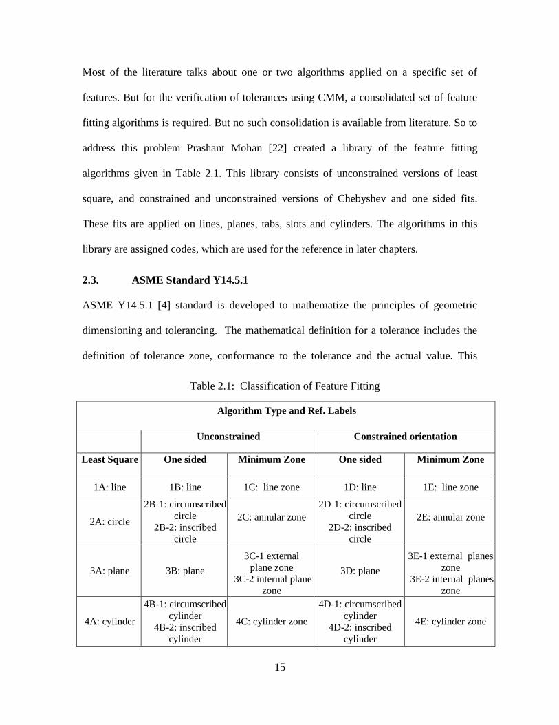
Table 2.1: Classification of Feature Fitting

Algorithm Type and Ref. Labels

Unconstrained Constrained orientation

Least Square One sided Minimum Zone One sided Minimum Zone

1A: line 1B: line 1C: line zone 1D: line 1E: line zone

2A: circle

2B-1: circumscribed

circle

2B-2: inscribed

circle

2C: annular zone

2D-1: circumscribed

circle

2D-2: inscribed

circle

2E: annular zone

3A: plane 3B: plane

3C-1 external

plane zone

3C-2 internal plane

zone

3D: plane

3E-1 external planes

zone

3E-2 internal planes

zone

4A: cylinder

4B-1: circumscribed

cylinder

4B-2: inscribed

cylinder

4C: cylinder zone

4D-1: circumscribed

cylinder

4D-2: inscribed

cylinder

4E: cylinder zone

Most of the literature talks about one or two algorithms applied on a specific set of

features. But for the verification of tolerances using CMM, a consolidated set of feature

fitting algorithms is required. But no such consolidation is available from literature. So to

address this problem Prashant Mohan [22] created a library of the feature fitting

algorithms given in Table 2.1. This library consists of unconstrained versions of least

square, and constrained and unconstrained versions of Chebyshev and one sided fits.

These fits are applied on lines, planes, tabs, slots and cylinders. The algorithms in this

library are assigned codes, which are used for the reference in later chapters.

2.3. ASME Standard Y14.5.1

ASME Y14.5.1 [4] standard is developed to mathematize the principles of geometric

dimensioning and tolerancing. The mathematical definition for a tolerance includes the

definition of tolerance zone, conformance to the tolerance and the actual value. This

16

standard presents a formal mathematical definition for each tolerance and a mathematical

inequality for conformance to this tolerance. The purpose of this standard is to serve as a

guide to the CMMs for the correct interpretation of standard definitions. But this standard

only gives a mathematical definition for tolerance. But it does not define how to reduce

the point set in a CMM to a substitute feature, that is, it does not define the type of

feature fitting algorithm to be used for reducing the point set.

17

CHAPTER 3

INTRODUCTION TO COORDINATE MEASURING MACHINES

3.1. Coordinate Measuring Machines

Coordinate Measuring Machines are the most versatile and widely used metrology

machines. They are flexible and accurate and help in decreasing the cost and time of

measurements. Their function is to measure the actual surface and identify the geometric

variations on this surface. Measurement of surface involves measuring characteristic

points on the surface. The points can be continuous or discrete and depends on type of

sensor used. These points are then processed to generate the substitute features for these

surfaces which can then be used for calculating geometric variations. Some important

advantages of CMM’s are: the need for aligning the part with reference frames is

eliminated, the need for gages, fixtures etc. is eliminated, all the size, form, orientation

and position requirements can be measured in a single setup [24].

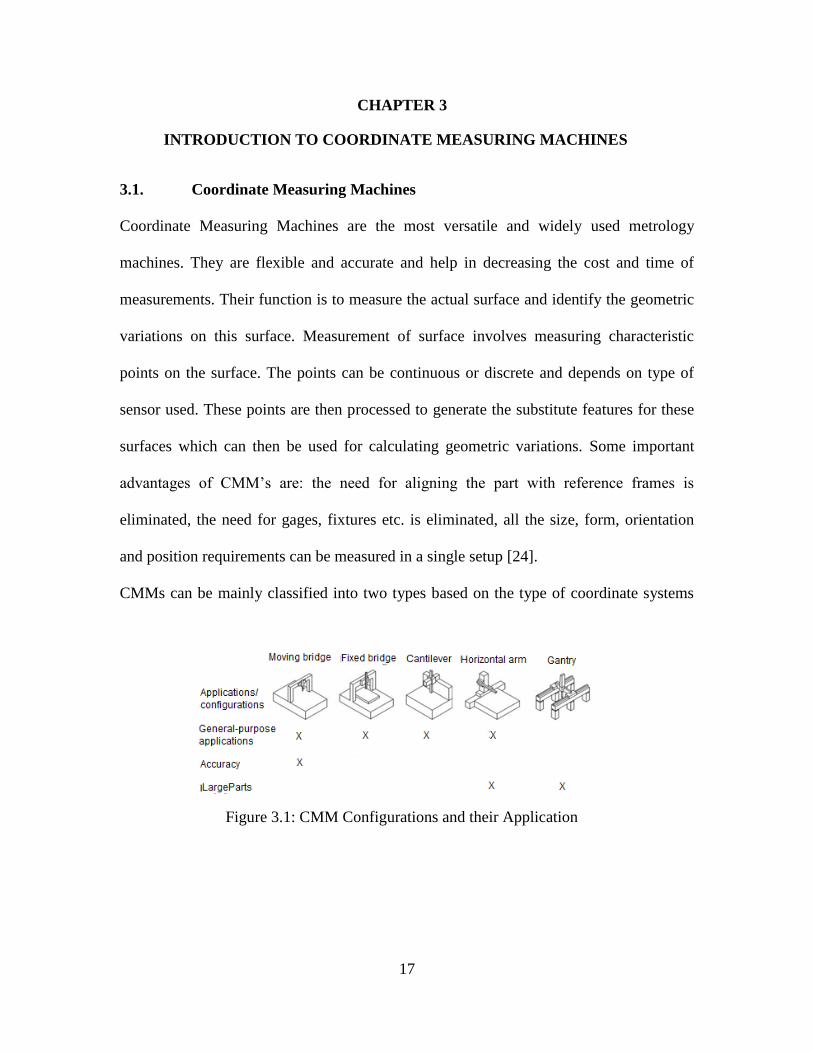
CMMs can be mainly classified into two types based on the type of coordinate systems

Figure 3.1: CMM Configurations and their Application

18

they are based upon. One is Cartesian coordinate systems and the other is Non-Cartesian

coordinate systems. Cartesian coordinate systems have rectilinear moving axes. The most

common configurations of this type are moving bridge, fixed bridge, cantilever,

horizontal arm and gantry [Figure 3.1]. These are considered to be more accurate and

reliable and are the widely used in industry. But with the increase in size of the parts to

be measured, the size and cost of these machines increases. Also the handling of the parts

becomes difficult.

Non Cartesian coordinate systems are composed of distributed components rather than

solid machines. Measurements are made using one of the several approaches: articulated

arms, triangulation method, spherical coordinate systems and multiple reference points.

The articulated arm CMM’s consist of several arms connected to each other and equipped

with angular encoders. The angles of rotation obtained from the angular encoders are

used to calculate the coordinates of the characteristic point.

3.2. Preliminary Tasks in a CMM

Even with the most advanced software and user interface, working with a CMM requires

knowledge and experience. To save time with programming and use of CMM six

preliminary tasks are recommended. The first task is observing the safety. Before starting

any measurements the bearing surface should be kept free of any objects used, keeping

all the manufacturer supplied covers, avoiding pinch points and keeping the pendant with

its emergency stop switch within reach. Proper lifting techniques should be used to place

and remove the work piece from the bearing surface.

The second task is starting the machine. Every machine has a check list given by the

manufacturer for startup. But there are few points that are common to every machine. The

19

bearing surfaces should be cleaned before use. All probes and stylus assemblies should be

ensured for tightness. CMM should be homed after every start up from power off state.

The third is identifying the GD&T and the surfaces to be inspected. Often there are few

critical features or key characteristics that are important than others. According to [24],

the programmer must look through the questions listed below before creating a plan for

inspection.

What datum features should be considered to construct the datum reference frames

for inspection.

Will it be possible to measure all the points in a single setup or the part should be

reoriented to reach all the features.

Are there groups of features that need to be evaluated as patterns?

Will it be possible to attain a small enough task specific measuring uncertainty for

each of the tolerances so that a 4:1 tolerance to uncertainty ratio can be achieved?

Fourth task is choosing the probes. The criterion for choosing the probes and styli is the

approachability of the features to be measured. They must be chosen such that all the

features can be measured with one probe stylus when possible. Addition of more probe

stylus combinations will increase the uncertainty in measurement. It is often better to

change the orientation of the part for better probe access than using a stylus configuration

that is awkward, unsteady or difficult to calibrate.

Fifth is fixturing. The parts need to be held rigidly. But the measuring forces are small.

So the fixtures need not be massive and restraining. One common technique is using

epoxy or super glue to fix the parts. Also the parts should be clamped away from the

CMM table to have good accessibility of all the part features. Otherwise multiple setups

20

might be required which increases both the measuring time and uncertainty. And the sixth

task is record keeping.

3.3. Working of a CMM

The first step is determination of the effective diameter and apparent form of the probe. It

is necessary to qualify the probes before using them for measurements. The second step

is the alignment process. The parts have to be aligned after qualification. Alignment is the

process of creating a coordinate system on the part. Alignment is a two-step process. At

first a rough coordinate system is created by measuring the points manually on the

features. Then a more accurate coordinate system is established by measuring the points

in automatic (DCC) mode. Sometimes the measurements in DCC mode are repeated to

get a stable and repeatable coordinate system. After establishing the coordinate systems,

datums are measured to establish the reference frame. If the parts are simple and have

only one DRF, the datum features will be used for generating the coordinate system. But

if the part has multiple DRF’s, multiple datums have to be measured. The next step

would be inspection. As the DRF’s and measurement strategies are developed

beforehand, inspection of the parts is easy. During inspection measuring features that are

nearer to each other will save time, even if they do not belong to same reference frame.

These measurements are then analyzed for tolerance verification. The analysis involves

fitting the substitute features and is sometimes done automatically using the least square

algorithms. On other times, user can choose the type of feature fitting algorithm to be

used for verifying the tolerance. The results of the analysis are presented in various ways.

The simplest is the text based output consisting of the list of features measured, the

attributes of the feature, tolerances on these attributes and a bar graph showing the

21

position of actual value in a tolerance band. Graphical outputs showing the location of the

actual feature in a CAD model are also available. But they take more time.

3.4. Test Run

It is better to make a test run after the program is complete. Test run helps to identify

collisions if any between the part and the probe. It is better to do the test runs at a slow

speed as it helps to avoid the damage of probe and parts. The test run also helps to go

through the report to check if all the features are measured, if proper tolerances are being

checked for the features and the format of the report.

22

CHAPTER 4

NORMATIVE PROCEDURES FOR COORDINATE

MEASURING MACHINES

4.1. Approach

As discussed in the previous chapter CMM’s evaluate tolerances by fitting a substitute

feature to the measured points. CMM’s provide two options to the user for the feature

fitting algorithms to be used. The first option is the default use of least squares algorithms

and the second option for user is the flexibility to choose the algorithm. But there are a

few concerns with these two approaches. The first one is “Do the least square fittings

confirm to the standard’s definition of tolerances?” The second one is “Does the use of

different algorithms give the same result? If not then which algorithm should be used for

evaluating a particular tolerance?” So to address this issue, in this research we are

proposing normative algorithms which provide the user with the best choice of feature

fitting algorithms to be used for verifying tolerances.

The normative algorithms that are being proposed are based on the interpretation of

standard definitions and the manual inspection practices. The ASME Y14.5 standard

gives clear definition of the tolerances and the rules for their application. Interpretation of

these definitions gives an understanding of the type of the feature fitting algorithms to be

used in CMM. For example, the standard defines form tolerances as zones that are free to

move within the limits set by size or orientation tolerances. So, to be in agreement with

this definition it would be appropriate to use an algorithm that fits a zone and is

unconstrained. Also, manual inspection practices have acted as a base for standard

23

definitions. So, these practices are also taken into consideration for proposing the

normative algorithms.

In the following sections each tolerance type is discussed one by one for the selection of

algorithms. Standard definitions and manual inspection practices are presented for each

case and are interpreted to see what type of feature fitting algorithm fits the particular

tolerance. Then based on these interpretations, suitable algorithm for verifying those

tolerances is selected from the library [Table 2.1]. It has been observed that not all the

manual inspection practices comply with standard definitions. The reason being that, it is

difficult to simulate the measuring conditions that satisfy the standard definition, as in

cylindricitiy. Also in some cases, the standard has multiple definitions, e.g. for size. In

such cases the choice of algorithms is based on design or assembly criterion.

4.2. Size

The term 'size' refers to the dimension applied to features of size. There are three features

of size- circle, cylinder and parallel faces that are most commonly used in any part. These

features of size form the interfaces between parts in an assembly. So the inspection of

these features plays an important role in determining the acceptability and assemblability

of these parts. It is also important to evaluate size for calculating bonus and shift

tolerances. The sections below give the details about standard definitions for size, manual

measurement process and the proposed normative algorithm for determining size in

CMMs. It is also necessary to mention that the definition of size is not unique and clear in

the standard. There are two different definitions for size. One is actual local size and the

other is actual mating size.

24

a. Standard Y14.5M Definitions

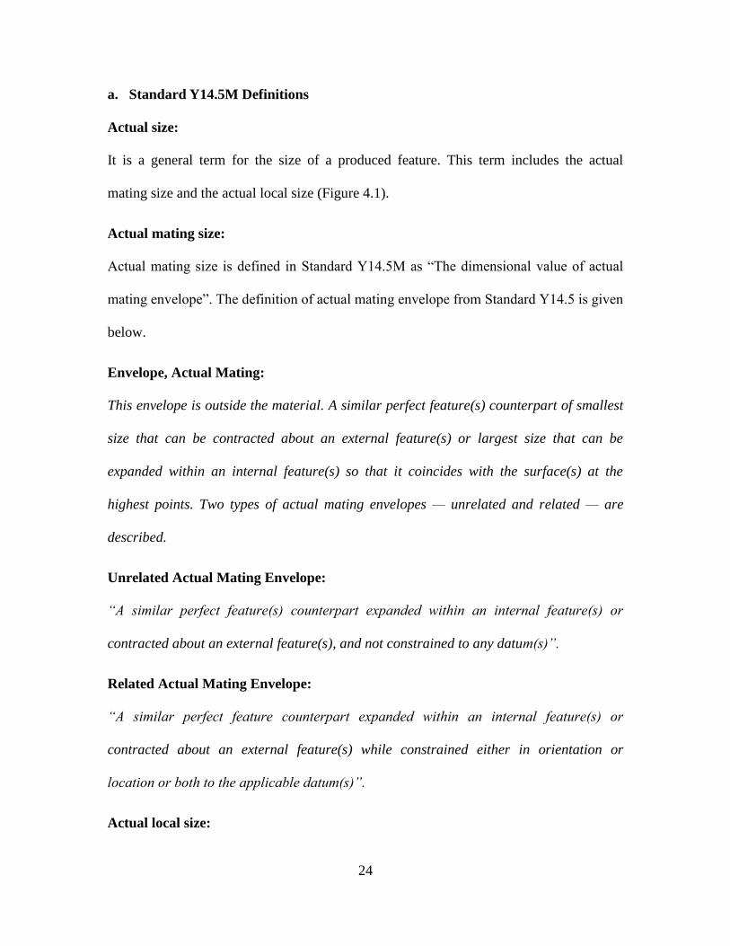
Actual size:

It is a general term for the size of a produced feature. This term includes the actual

mating size and the actual local size (Figure 4.1).

Actual mating size:

Actual mating size is defined in Standard Y14.5M as “The dimensional value of actual

mating envelope”. The definition of actual mating envelope from Standard Y14.5 is given

below.

Envelope, Actual Mating:

This envelope is outside the material. A similar perfect feature(s) counterpart of smallest

size that can be contracted about an external feature(s) or largest size that can be

expanded within an internal feature(s) so that it coincides with the surface(s) at the

highest points. Two types of actual mating envelopes — unrelated and related — are

described.

Unrelated Actual Mating Envelope:

“A similar perfect feature(s) counterpart expanded within an internal feature(s) or

contracted about an external feature(s), and not constrained to any datum(s)”.

Related Actual Mating Envelope:

“A similar perfect feature counterpart expanded within an internal feature(s) or

contracted about an external feature(s) while constrained either in orientation or

location or both to the applicable datum(s)”.

Actual local size:

25

The value of any individual distance at any cross section of a feature measured between

two points located opposite to each other.

b. Manual Inspection Methods

The size of a shaft is measured at various cross sections and the maximum reading is

considered the diameter of the shaft. Similarly for a hole, the minimum value of the

measurements taken at various cross sections gives the diameter of the hole. These

measurements are usually made with vernier scales and micrometers.

c. Justification

As described above, the standard gives multiple definitions for size, the actual local size

and the actual mating size. To determine the acceptance of a part, both of them have to be

evaluated. Actual mating size can be measured with a CMM. But it is not easy to

measure actual local size. Actual local size is the distance between two diametrically

opposite points. To find this with a CMM the user has to measure two diametrically

opposite points on a cross section. But, locating the diametrically opposite points on a

cross section is not possible with the available feature fitting algorithms in a CMM. On

Figure 4.1: Size Definition

26

the other hand, it is relatively easy to measure local sizes manually. So, it is advised to

measure local sizes manually.

Comparing the two definitions of size, from assemblability point of view, actual mating

size is important. This size is important as it is used in determining the bonus and shift

tolerances. This size is also useful in verifying the parts conformance to Rule #1 in

standard.

Actual mating size refers to the size of envelope that touches the actual feature at the

extreme most points. If the feature is external, the envelope touches the outermost points

and encloses all the points on the feature. If the feature is internal the envelope touches

the innermost points. The feature fitting algorithms that best suit this are the one sided

fits. For an external feature, minimum circumscribed fit should be used and for an

internal feature, maximum inscribed feature should be used. For width features, the

related fit would be minimum zone internal fit for an internal feature and minimum zone

external for an external feature. The proposed normative procedure for verifying size on

different features of size is explained below.

d. Proposed Normative Algorithms

Cylindrical Features:

1) Measure the points on the cylindrical feature.

2) If the feature is internal use unconstrained Maximum Inscribed fit (algorithm 4B-2,

Table 2.1) and if the feature is external use unconstrained Minimum Circumscribed fit

(algorithm 4B-1, Table 2.1).

3) The diameter of these one sided fits gives the size of that feature.

Figure 4.2 shows the unconstrained and constrained fits for hole to evaluate size.

27

Slot and Tab:

1) Measure points on both the faces of the slot or tab which form the FOS.

2) For a tab, consider the points on both the surfaces as one set and then fit an

unconstrained two sided plane fit (algorithm 3C-1, Table 2.1) which is external to the

points.

3) For a slot, fit an unconstrained two-sided plane fit (algorithm 3C-2, Table 2.1) which

is internal to the measured points.

4) The distance between the two planes gives the size of the tab or slot.

If the feature of size is target or primary datum, above algorithms should be used without

any constraints applied to the feature. But, if the feature of size is a secondary or tertiary

datum, necessary constraints have to be applied to the feature. Figure 4.3 shows

unconstrained and constrained fits for a slot.

Figure 4.2: Size of Unconstrained and Constrained Hole

28

Note: The size obtained from unconstrained fits includes form tolerance, and constrained

fits includes orientation tolerance.

4.3. Form Tolerances

Form tolerances are the group of tolerances that control the surface characteristics of a

feature. These are straightness, circularity, flatness and cylindricitiy. These tolerances are

not referenced to any datums. Following rule #1 in the standard, they are free to rotate

and translate within the limits set by size. [Rule #1 says that the form tolerance should

not exceed the MMC limit on a feature.] In standard Y14.5, these tolerances are defined

as zones. Each of the form tolerances is discussed in the following sections with respect

to the standard definitions, manual measurement practices and proposed normative

procedures.

Straightness 4.3.1.


Cylindrical features

According to the standard, each longitudinal element of the cylindrical surface must lie

within the straightness limits and also the size of the feature should be within the limits,

without violating the MMC condition. The definition as given in the standard is described

below:

Figure 4.3: Size of Constrained and

Unconstrained Slot

29

“Each longitudinal element of the surface must lie between two parallel lines separated

by the amount of the prescribed straightness tolerance and in a plane common with the

axis of the unrelated actual mating envelope of the feature. (Figure 4.4)”

Planar features

The line elements must lie in a tolerance zone between two lines separated by the

straightness tolerance (Figure 4.5). The direction of line elements depends on the view of

drawing on which callout is specified. The tolerance zone can tilt and shift within the size

tolerance to accommodate gross surface undulations.


Straightness for cylindrical parts is measured using jack screws and dial indicator. To

measure straightness few line elements are randomly selected on the surface. Then the

straightness error for each line element is calculated separately. The line element on the

Figure 4.5: Straightness on a Planar Surface

Figure 4.4: Straightness on Cylindrical Feature

30

surface is adjusted to be parallel to surface plate using jackscrews. Then straightness is

measured using a dial indicator. The full indicator movement of the dial indicator gives

the straightness error of the line element. The process is repeated for four times at

different angular locations and the maximum value of full indicator movement obtained

is considered as the straightness error. Straightness can also be measured using a

straightedge and feeler wires. For non-cylindrical parts e.g., a cone, straightness is

measured using jackscrew and dial indicator following the same procedure of cylindrical

parts.

c. Justification

To evaluate straightness on a cylindrical or planar surface the points are measured on the

surface along a straight line (approximately). These measurements have to be taken on

multiple lines. The number of lines is dependent on the quality of manufacturing process

used for producing the part and is beyond the scope of this book. But a minimum of four

lines is proposed in the normative algorithm based on the reference [3].

According to the standard definition, straightness is defined as a zone formed by two

parallel lines, which encapsulate all the measured points and are separated by a minimum

distance possible. A zone can be calculated using both the least squares fit and minimum

zone fits. But among these two the minimum zone fits give a minimum value to the

zones. So an unconstrained minimum zone line fit is used to evaluate the straightness. For

using this fit, the points measured must be in a plane. But the points measured using the

CMM are dispersed in 3D space. So they are projected onto a plane before using the

feature fitting algorithm. From the standard, this plane should pass through the axis of

unrelated mating envelop of the cylinder. To find the unrelated mating envelope, an

31

unconstrained maximum inscribed cylinder has to be used for hole and an unconstrained

minimum circumscribed cylinder has to be used for pin.

For planar surface, the procedure is same, except that the plane on which the points are

projected is in alignment with the CAD drawing of the part. The normative procedure

proposed outlines the process for calculating the straightness.

d. Proposed Normative Algorithms

Cylindrical features:

1) Measure points on the surface of cylinder (external feature) along a straight line

(Figure 4.6: Straightness of Surface (a)).

2) Repeat the measurements to a minimum of four lines that span the surface.

3) Fit an unconstrained minimum circumscribed cylinder to the points using algorithm

4B-1 from Table 2.1.

Figure 4.6: Straightness of Surface

32

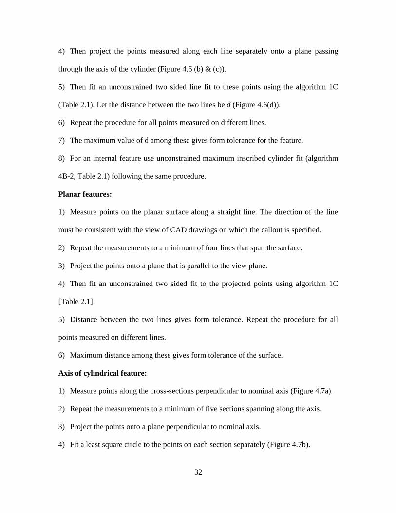
4) Then project the points measured along each line separately onto a plane passing

through the axis of the cylinder (Figure 4.6 (b) & (c)).

5) Then fit an unconstrained two sided line fit to these points using the algorithm 1C

(Table 2.1). Let the distance between the two lines be d (Figure 4.6(d)).

6) Repeat the procedure for all points measured on different lines.

7) The maximum value of d among these gives form tolerance for the feature.

8) For an internal feature use unconstrained maximum inscribed cylinder fit (algorithm

4B-2, Table 2.1) following the same procedure.

Planar features:

1) Measure points on the planar surface along a straight line. The direction of the line

must be consistent with the view of CAD drawings on which the callout is specified.

2) Repeat the measurements to a minimum of four lines that span the surface.

3) Project the points onto a plane that is parallel to the view plane.

4) Then fit an unconstrained two sided fit to the projected points using algorithm 1C

[Table 2.1].

5) Distance between the two lines gives form tolerance. Repeat the procedure for all

points measured on different lines.

6) Maximum distance among these gives form tolerance of the surface.

Axis of cylindrical feature:

1) Measure points along the cross-sections perpendicular to nominal axis (Figure 4.7a).

2) Repeat the measurements to a minimum of five sections spanning along the axis.

3) Project the points onto a plane perpendicular to nominal axis.

4) Fit a least square circle to the points on each section separately (Figure 4.7b).

33

5) Find the centers of all the sections and fit an unconstrained minimum cylinder fit to

these centers (Figure 4.7c).

6) The diameter of the cylinder gives the straightness error of the axis.

Flatness of a Surface 4.3.2.

a. Standard Y14.5 Definition

“Flatness is the condition of a surface having all elements in one plane. A flatness

tolerance specifies a tolerance zone defined by two parallel planes within which the

surface must lie” (Figure 4.8).

Figure 4.8: Flatness of a Surface

Figure 4.7: Straightness of Axis

34


Flatness is measured using jackscrew and dial indicator. The surface is held parallel to

the surface plate by adjusting jackscrews. Then dial indicator is traversed over the entire

surface and the full indicator movement gives the flatness measurement. For measuring

tight tolerances optical flats are used.

c. Justification

The standard defines the flatness tolerance as a zone. And it is free to rotate within the

limits of size. The manual inspection practices also simulate a zone by measuring the

measuring the distance between farthest and nearest points on the surface. So considering

both the standard and manual inspection practices an unconstrained zone fit would be

suitable for measuring flatness. The corresponding algorithm from Table 2.1 is

unconstrained external minimum zone plane fit (3B-1).

d. Proposed Normative Algorithm

1) Measure points spanning the planar surface whose flatness is to be determined.

2) Fit an unconstrained minimum zone plane fit (algorithm 3B-1, Table 2.1) external to

the points measured on the surface.

3) The distance between two planes gives the flatness variation of the surface.

Flatness of a Median Plane 4.3.3.


Flatness is the condition of a derived median plane having all elements in one plane. A

flatness tolerance specifies a tolerance zone defined by two parallel planes within which

the derived median plane must lie (Figure 4.9). The individual elements of the feature

should be within the given size limits.

35

b. Justification

According to the standard, the points on the derived median plane should be within the

specified tolerance. But, the problem is finding the derived median plane. The points on

the derived median are the midpoints of features actual local sizes. But, it is not possible

to measure actual local sizes using the CMMs. So, to overcome this problem, the

following method is proposed. A grid of perpendicularly intersecting lines is overlaid on

both the end faces of the feature. Coordinate measurements are made at the intersections

of the grid lines on both the surfaces. Then the points on the median plane are obtained

by calculating the mid values of the correspondingly opposite points on the surfaces.

c. Proposed Normative Algorithm

For measuring the flatness of median plane, the following procedure is suggested.

1) Overlay a grid of intersecting lines (solid lines in Figure 4.10) on both the surfaces of

the feature.

2) Take coordinate measurements at the intersection of the grid lines on both the

surfaces.

Figure 4.9: Flatness of Medial Plane.

36

3) Calculate the midpoints of the corresponding opposite points of the surfaces.

4) Fit a two sided external plane zone to the midpoints using the algorithm 3C-1 (Table

2.1).

5) The distance between the two planes of the zone gives the flatness of the medial

plane.

Figure 4.10 shows the grid layout for the part given in Figure 4.9.

Cylindricity 4.3.4.

a. Standard Y14.5M Definition

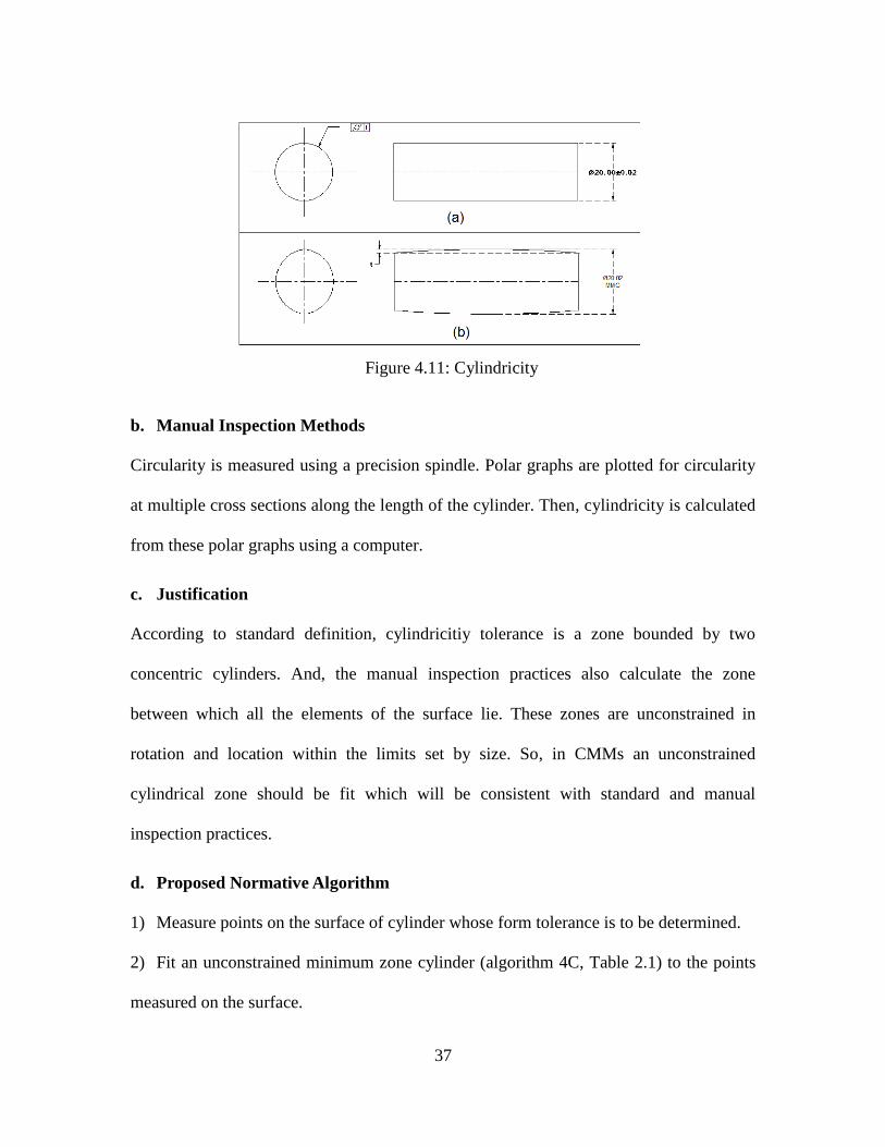
“A cylindricity tolerance specifies a tolerance zone bounded by two concentric cylinders

within which the surface must lie” (Figure 4.11).

Figure 4.10: Block Layout for Flatness

measurement

37


Circularity is measured using a precision spindle. Polar graphs are plotted for circularity

at multiple cross sections along the length of the cylinder. Then, cylindricity is calculated

from these polar graphs using a computer.

c. Justification

According to standard definition, cylindricitiy tolerance is a zone bounded by two

concentric cylinders. And, the manual inspection practices also calculate the zone

between which all the elements of the surface lie. These zones are unconstrained in

rotation and location within the limits set by size. So, in CMMs an unconstrained

cylindrical zone should be fit which will be consistent with standard and manual

inspection practices.


1) Measure points on the surface of cylinder whose form tolerance is to be determined.

2) Fit an unconstrained minimum zone cylinder (algorithm 4C, Table 2.1) to the points

measured on the surface.

Figure 4.11: Cylindricity

38

3) The radial distance between the two concentric cylinders gives the cylindricity error.

Circularity 4.3.5.


“Circularity tolerance specifies a tolerance zone bounded by two concentric circles

within which the circular element of the surface must lie, and applies independently at

any plane described below. For a feature other than a sphere, the plane is perpendicular

to an axis or spine (curved line) of the feature and for a sphere, the plane that passes

through a common center (Figure 4.12)”


Circularity is measured using V-block and a dial indicator. The angle of V-block to be

used for measurement is calculated from the number of lobes on the part. A precision

spindle can be used to measure the number of lobes on the part surface. For measuring

circularity, the part is mounted on the V-block and the dial indicator is placed on top dead

center of the part. Now, the part is rotated through 180°. The dial indicator movement

obtained is divided by the appropriate correction factor to find the circularity error at that

section. The process is repeated at various (minimum of four) sections and the maximum

of the errors obtained is considered as circularity error of the part.

Figure 4.12: Circularity for a Cylinder

39

c. Justification

In manual inspection, the circularity is measured by calculating the difference between

maximum and minimum diameters. And, the diameters are assumed to be concentric with

each other in this process. So, this process gives a zone bounded by two concentric

circles. The inner diameter of the zone is the minimum diameter and the outer diameter of

the zone is the maximum diameter.

The standard also says that the circular element at any given cross section must lie

between two concentric circles. In the definition, it is also mentioned that the section in

which points are measured must be perpendicular to the actual axis\spine. But,

considering the amount of straightness deviation allowed on the axis, the error that results

by making the measurements in the planes perpendicular to the nominal axis will be

negligible. Also, the type of zone that is to be fitted to the measured points on the cross

section is not mentioned in the standard. But, based on the recommendations in standard

B89.3.1 [25] for measurement of roundness errors, minimum zone is used for evaluating

circularity of error.


1) Measure the points on various cross sections that are perpendicular to the nominal

axis.

2) Project the points at each cross section onto a plane that is perpendicular to the

nominal axis.

3) Then fit a minimum zone circle fit to these projected points (algorithm 2C, Table

2.1).

4) Let the radial distance between two circles of the fit be d.

40

5) Repeat this for the points measured at other cross sections also. The maximum of the

distances d gives the circularity error of the feature.

4.4. Orientation Tolerances

Orientation tolerances control parallelism, perpendicularity and angularity of a feature.

These tolerances control the rotational degrees of freedom of a feature. They do not

control translation. The orientation tolerances control the form of the feature to the extent

of orientation tolerance. But, they do not control location of the feature. Since, these

tolerances do not control translational degrees of freedom, the feature being controlled is

only oriented to the datum reference frame. Multiple datums might be required to control

the required rotational degrees of freedom depending on the number of degrees of

freedom controlled by each.

The standard specifies four types of tolerance zones for orientation tolerances. These four

types differ in the type of target features being controlled. The datum features are either

planes or cylinders in all the cases. And the tolerance zones are oriented at the specified

angle or parallel or perpendicular to the datums. These four types as defined by the

standard are:

1) A tolerance zone defined by two parallel planes within which the surface or center

plane of the controlled feature must lie.

2) A tolerance zone defined by two parallel planes within which the axis of the

controlled feature must lie.

3) A cylindrical tolerance zone within which the axis of the controlled feature must lie.

4) A tolerance zone defined by two parallel lines within which the line element of the

surface of must lie.

41

Parallelism 4.4.1.


The standard defines parallelism as a condition in which the target plane or axis is

equidistant to a datum feature at all points. And the parallelism tolerance is defined as a

zone parallel to a datum plane or axis within which the surface or center plane or axis of

the feature must lie. The tolerance zone is either defined by a cylinder or two parallel

planes and this depends on the type of datum and target features (Figure 4.13 & Figure

4.14).

Figure 4.14: Parallelism Defined by a Cylindrical Zone

Figure 4.13: Parallelism Defined by Zone Bounded by

Two Parallel Planes

42


The manual measurement methods for the inspection of parallelism are aimed at

measuring the width of the zone within which all the surface elements of the controlled

feature lie. In case of planar features this is achieved using a surface plate and a dial

indicator. And, in case of cylindrical features this is achieved using gage pins and dial

indicator. The orientation of the measured zone is held parallel to the datum feature in

both the cases. The process of inspection for both types of features is detailed in the

following paragraphs.

Planar Features

Parallelism is measured by using a surface plate and a dial indicator. The part is placed

on the surface plate with datum surface facing the surface plate. Then a dial indicator is

traversed over the surface for which parallelism is to be determined. The full indicator

movement of the dial indicator gives the parallelism error.

Cylindrical Features

To measure the parallelism of the axis of a cylinder, a gage pin of largest possible size is

inserted into the cylindrical feature. Then, using the dial indicator, readings are taken

over the top dead center of the pin next to the hole on both sides. The difference between

the two readings gives the parallelism error. In case the datum is a cylindrical feature

rotate the setup through 90° and repeat the experiment. The root of sum of squares of the

two values gives parallelism error.

c. Justification

To measure parallelism of any feature, datum features need to be established first. Datum

feature can be a plane or a cylinder or a width feature. In manual inspection practices

43

datums are simulated by placing the datum feature on a nearly perfect counterpart. This

counterpart touches the datum features at its highest points. So, to simulate datums in a

CMM following the same principle, planar features have to be fit with one sided

unconstrained plane fit, cylindrical datums have to be fit with unconstrained maximum

inscribed or minimum circumscribed fit and width features with unconstrained internal or

external minimum zone plane fit. These fits also comply with the 3-2-1 rule described in

standard for datums.

According to the standard, parallelism is defined as the condition of target feature being

equidistant from the datum feature at all points. So to measure parallelism, the deviation

of the points on target feature from the datum feature has to be measured. For a planar

feature, with a planar datum, the difference of the farthest and nearest points on the

feature from the datum gives this deviation. For a cylindrical feature, with a planar

datum, the deviation of the axis from the datum feature gives the parallelism error.

According to the standard this axis should be derived from an unconstrained one sided fit.

This also complies with the manual inspection practices, which use a gauge pin of

maximum possible size for verifying parallelism.


Planar Features

1) Measure points on both the datum plane and target plane.

2) Fit an unconstrained one sided plane fit to the points on the datum plane using the

algorithm 3B.

3) Then find the farthest and nearest points of the target feature from the datum plane.

4) The distance between the two points gives the parallelism error.

44


1) Measure the points on both datum and target surfaces (Figure 4.15b, Figure 4.16c).

2) If datum is a planar feature,

a) fit an unconstrained one sided plane to the points using the algorithm 3B.

b) Now fit an unconstrained one sided fit to the points on the target feature- MC cylinder

if the feature is external (algorithm 4B-1) or MI cylinder if the feature is internal

(algorithm 4B-2) (Figure 4.15d).

Following the standard definition for parallelism tolerance, a parallel plane zone has to be

fit to the axis of the cylinder. Then the width of zone gives the parallelism error. Instead

the same error can be obtained by projecting the length of axis on to the normal of the

datum plane. The latter method for calculating the parallelism error reduces the

computation.

c) Project the axis of the cylinder on to the normal of the datum plane. The length of the

projection gives the parallelism error (Figure 4.15e).

3) If the datum is a cylindrical feature, then:

a) fit an unconstrained minimum circumscribed cylinder to the points if the feature is

external (algorithm 4B-1, Table 2.1) or maximum inscribed cylinder if the feature is

internal (algorithm 4B-2) (Figure 4.16d).

Figure 4.15: Measurement of Parallelism of a Cylinder Parallel to a Datum

plane

45

b) Now fit another unconstrained one sided fit to the points on the target feature (Figure

4.16d).

According to the standard definition, a cylindrical zone has to be fit to the axis of the one

sided fit. And, the diameter of the zone gives the parallelism error. Instead, the axis is

projected on to the plane perpendicular to the datum feature and the length of projection

gives parallelism error.

c) Project the axis of the cylinder on to the plane perpendicular to the datum feature. The

length of projection gives the parallelism error (Figure 4.16e).

For cylindrical datum features unconstrained one sided fit (ref: section 4.11.4 (a) of

standard Y14.5M) has to be used.

Figure 4.16: Measurement of Parallelism of a Cylinder Parallel to a

Cylindrical Datum

46

Perpendicularity 4.4.2.


According to the standard, perpendicularity tolerance specifies a tolerance zone

perpendicular to a datum plane or axis within which the surface or center plane or axis of

the feature must lie. The tolerance zone is either cylindrical (Figure 4.18) or bounded by

two parallel planes (Figure 4.17) and the choice depends on target feature.

Figure 4.18: Perpendicularity Specified for a Planar Surface

Figure 4.17: Perpendicularity Specified to a Cylinder

47


The manual measurement methods for measuring perpendicularity aim at finding the

minimum width of zone within which all the points on the controlled surface lie. The

orientation of the measured zone is maintained perpendicular to the datum. The

measurement methods are different for planar and cylindrical features. In the case of

planar features, the measurement is made using surface plate and dial indicator. And, for

cylindrical features the measurements are made using gage pin and dial indicator. The

details of inspection are detailed below.

Planar Features

Perpendicularity is measured by using a surface plate and a dial indicator. The part is

placed on the surface plate with datum surface facing the surface plate. Then a dial

indicator is traversed over the surface for which perpendicularity is to be determined. The

part is rocked until a minimum reading is obtained. The minimum of full indicator

movements of the dial indicator gives the perpendicularity error.


To measure the perpendicularity of a cylinder, a gage pin of largest possible size is

inserted into the cylindrical feature. Then, using the dial indicator, readings are taken

over the top dead center of the pin, next to the hole, on both sides. Then the setup is

rotated through 90° to repeat the measurement. The root of sum of squares of the two

values gives parallelism error. If the datum feature is a cylinder, then measurements are

done only in one orientation and difference between the readings is considered as the

perpendicularity error.

48

c. Justification

Verification of perpendicularity first requires the simulation of datums and then the target

features. The datums can be any of the features of plane, cylinder or parallel faces. Datum

simulation is again done using one sided unconstrained fits to match the standard

definition and manual inspection practices.

Perpendicularity tolerance, in the standard, is defined as a zone of minimum thickness

that encloses all the points on the feature and is perpendicular to datums [4]. The manual

measurement methods also find the minimum possible width, perpendicular to the datum

that encloses all the points on the measured surface. In both the standard and the manual

inspection practices, perpendicularity tolerance is considered as a zone that is constrained

perpendicular to the datums. The feature fitting algorithm that gives such a zone for

planar features is the constrained external minimum zone plane fit.

For cylindrical features, perpendicularity is measured for the derived features. So these

derived features have to be found, before calculating the perpendicularity. These derived

features can be found either by using the least square fits or one sided fits or the

minimum zone fits. As per the standard definitions unconstrained actual mating

envelopes have to be used to calculate these derived features. The manual inspection

practices also use gauge pins and precision parallels of maximum possible width in

measuring the tolerances. These instruments agree with the actual mating envelop

definition of the standard. So, in CMMs, actual mating envelopes have to be simulated.

And the feature fitting algorithms that fit this purpose are: unconstrained minimum

circumscribed cylinder for pins, unconstrained maximum circumscribed cylinder for

49

holes. The following paragraphs detail the normative procedures for CMM using the

above fits.


Planar Features


2) Fit a one sided plane fit to the points on the datum plane using the algorithm 3B.

3) Then fit a minimum zone fit external to the points on the target plane constrained

perpendicular to the datum plane using the algorithm 3E-1.

4) If there are multiple datums in the feature control frame, then the zone has to be

constrained to all the datums.

5) The distance between the planes of minimum zone obtained gives the

perpendicularity error.


1) Measure the points on both datum and target surfaces.

2) If the datum is a planar surface, then:

a) fit an unconstrained one sided plane to the points on the datum plane (algorithm 3B,

Table 2.1).

b) Fit an unconstrained minimum circumscribed cylinder if the feature is external

(algorithm 4B-1) and an unconstrained maximum inscribed cylinder if the feature is

internal (algorithm 4B-2, Table 2.1).

c) Project the axis of this one sided fit on to the datum plane. The length of projected

axis gives the perpendicularity error.

3) If the datum feature is a cylinder, then:

50

a) Fit an unconstrained minimum circumscribed cylinder to the datum points if the

feature is external (algorithm 4B-1, Table 2.1) and a maximum inscribed cylinder if the

feature is internal (algorithm 4B-2, Table 2.1).

b) Now fit an unconstrained one sided fit to the points on the target feature. Project the

axis of this unconstrained fit on to the axis of datum feature.

c) The projected length of the axis gives the perpendicularity error.

Angularity 4.4.3.

a. Standard Y14.5M definitions

An angularity tolerance specifies a tolerance zone oriented at the given angle to a datum

plane or axis within which the surface or center plane or axis of the feature must lie. The

tolerance zone is either cylindrical or defined by two parallel planes and the choice

depends on target feature (Figure 4.20 & Figure 4.19). The surface or the axis of the

feature must lie within the specified tolerance limits.


Figure 4.19: Angularity Specified on a Cylinder

51

Similar to parallelism and perpendicularity, the manual measurement methods for

measuring angularity also find the thickness of the zone that encloses all the points on a

target surface. For measuring angularity on planar surfaces, a dial indicator and a sine bar

are used. For measuring cylindrical features, gage pins and dial indicator are used.

Planar Features

Angularity is measured by using a surface plate, sine bar and a dial indicator. The part is

placed on the sine bar with datum surface on the sine bar. And, the part is held such that

the target feature is parallel to the surface plate. Then, a dial indicator is traversed over

the surface for which perpendicularity is to be determined. The part is rocked until a

minimum reading is obtained. The minimum of full indicator movements of the dial

indicator gives the angularity error.


To measure the perpendicularity of axis of cylinder, a gage pin of largest possible size is

inserted into the cylindrical feature. Then, using the dial indicator, take readings over the

top dead center of the pin next to the hole on both sides. Calculate the difference between

Figure 4.20: Angularity Specified for a Planar Surface

52

two readings. Rock the part until a minimum value of the difference between the readings

is obtained.

c. Justification

Similar to parallelism and perpendicularity, angularity tolerance is also defined as a zone.

And the angularity error is defined as the width of a zone of smallest possible thickness

that can enclose all the points on the feature being controlled. The zone is oriented to the

datum. The manual measurement methods also evaluate the same. So, in CMMs a feature

fitting algorithm that gives a constrained minimum zone has to be used. This can be

achieved using the constrained minimum zone fits for a plane.

For a feature of size, angular tolerance is applicable to the derived feature. As per the

standard definition this derived feature must be calculated from an unconstrained mating

envelope. In the manual inspection practices, gauge pins or adjustable precision parallels

are used to calculate the angularity. These boundary measured by these instruments is

equivalent to the unconstrained mating envelop definition of the standard. To be in

conformance with the standard and the manual inspection practices, an unconstrained

mating envelop has to be used for calculating the derived features in CMMs. The feature

fitting algorithms for cylinders that best suit this purpose are unconstrained maximum

inscribed cylinder for hole and unconstrained minimum circumscribed cylinder for pin.

The algorithms in the next two paragraphs describe how to evaluate angularity on planar

and cylindrical features using these fits.


Planar Features


53

2) Fit an unconstrained one sided plane fit to the points on the datum plane using the

algorithm 3B in Table 2.1.

3) Then fit a constrained minimum zone fit external to the points on the target plane

oriented at required angle to the datum plane using the algorithm 3E-1, Table 2.1.

4) If there are multiple datums in the feature control frame, then the zone has to be

constrained to all the datums.

5) The distance between the planes of minimum zone gives the angularity error.


1) Measure the points on both datum and target surfaces.

2) If the datum is a planar feature, then:

a) Fit an unconstrained one sided plane to the points on the datum plane using the

algorithm 3B, Table 2.1.

b) Now fit a minimum circumscribed cylinder to the points on the cylindrical target

feature if the feature is external (algorithm 4B-1, Table 2.1) or a maximum inscribed

cylinder if the feature is internal (algorithm 4B-2, Table 2.1).

c) Find a plane oriented perpendicular to the nominal axis of the target feature. The

projected length of the axis on to the new plane gives the angularity error.

3) If the datum feature is a cylinder, then:

a) fit an unconstrained minimum circumscribed cylinder to the points on datum feature

if the feature is external (algorithm 4B-1, Table 2.1) or a maximum inscribed cylinder if

the feature is internal (algorithm 4B-2, Table 2.1).

b) Fit an unconstrained one sided fit to the points on the target feature.

54

c) Then find a plane oriented perpendicular to the nominal axis of the target feature. The

projected length of the axis on to the new plane gives the angularity error.

d) If the tolerance zone is not cylindrical then find a perpendicular to the datum that lies

in the plane normal to the nominal axis. The projected length of the axis of the target

feature along this perpendicular gives the angularity error.

4.5. Position Tolerance


According to standard a positional tolerance defines either of the following:

(a) a zone within which the center, axis, or center plane of a feature of size is permitted to

vary from a true (theoretically exact) position

(b) (where specified on an MMC or LMC basis) a boundary, defined as the virtual

condition, located at the true (theoretically exact) position, that may not be violated by

the surface or surfaces of the considered feature of size.

Figure 4.21 shows position tolerance applied on a hole. The feature is referenced to three

planar datums labelled A, B and C. The hole is toleranced using RFS condition.

Figure 4.21: Positional Tolerance

55


The position tolerance can be measured using a gage pin of largest size that can be

inserted into the hole, a dial indicator and a surface plate. During measurement, the pin is

inserted into the hole such that it does not protrude past the datum. The part is mounted

onto the accessories such that the pin is horizontal. The distance of the top of the gage pin

at the ends of the hole is measured from the appropriate datum surface. Then the part is

rotated through 90° and the distance of the top of the gage pin is measured from the other

datum. By subtracting one-half the size of pin and the basic dimensions from the

readings, the position deviations for hole are obtained along two perpendicular directions.

The root of sum of squares of position deviations gives the diameter of the position

tolerance.

c. Justification:

Position tolerance is applicable to features of size and is referenced to datums. So, in a

CMM to find the position tolerance, it is necessary to find datum features first. To

simulate datums, one sided fits are used. These one sided fits comply with the standard

and the manual inspection practices.

Position tolerance is defined as a zone, applicable for derived features of features of size.

The derived feature for cylinder is axis and for width features is mid plane. There are

three types of these feature fittings that are available for calculating these feature fittings -

least square, minimum zone and one sided fits. Each of them gives a different result from

the other. So to decide on the normative procedure to be used, the standard and the

manual inspection practices are interpreted. As per the standard, unconstrained actual

mating envelop should be used for calculating the derived features. And in manual

56

inspection practices, gauge pins and adjustable parallels are used. These instruments

reciprocate the actual mating envelope of the standard definitions. So the actual mating

envelope should be used in CMM measurements. Of the three feature fittings, one sided

fits are suitable for cylinders and minimum zone fits are suitable for parallel faces. For a

pin it is minimum circumscribed cylinder, for a hole it is maximum inscribed cylinder,

for a tab it is external minimum zone plane fit, for a slot it is internal minimum zone fit.

All these fits should be unconstrained. After finding the derived features, the position

tolerance should be calculated by fitting zones to the derived features. Since these derived

features are calculated using feature fittings, we have the mathematical parameters

associated with them. These mathematical parameters are used for finding the zones

directly, instead of using the feature fitting algorithms. The details of finding the zones

are given in the algorithm below.


1) Measure points on the datum and target features spanning the surface.

2) For datum and target features use the feature fitting algorithms listed in the Table 4.1

and Table 4.2.

3) After feature fitting to targets, calculate the plane that is at a distance equal to the

nominal height of the feature of size.

4) Then find the intersection points of the axis/mid plane of target feature with the

datum plane.

5) The distance of the farthest point of intersection from nominal axis\mid plane (r1 in

Figure 4.22) gives half the position tolerance.

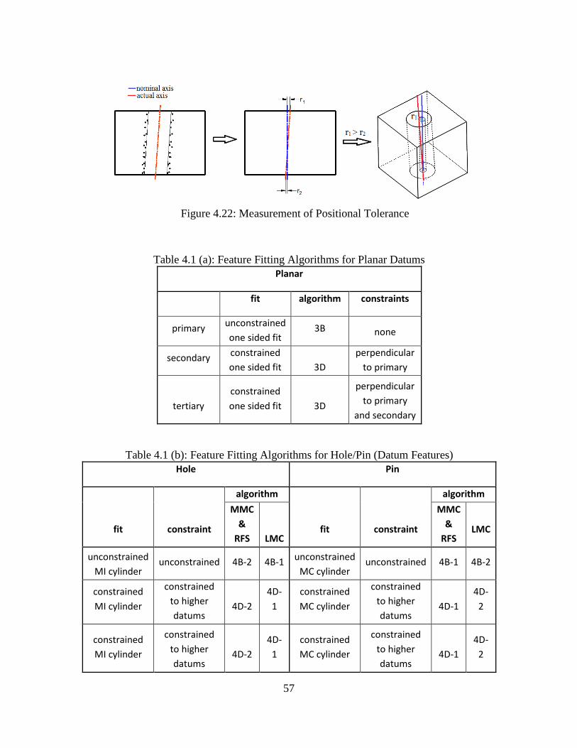
57

Figure 4.22: Measurement of Positional Tolerance

Table 4.1 (a): Feature Fitting Algorithms for Planar Datums

Planar

fit algorithm constraints

primary unconstrained

one sided fit 3B none

secondary constrained

one sided fit 3D

perpendicular

to primary

tertiary

constrained

one sided fit 3D

perpendicular

to primary

and secondary

Table 4.1 (b): Feature Fitting Algorithms for Hole/Pin (Datum Features)

Hole Pin

fit constraint

algorithm

fit constraint

algorithm

MMC

&

RFS LMC

MMC

&

RFS LMC

unconstrained

MI cylinder unconstrained 4B-2 4B-1 unconstrained

MC cylinder unconstrained 4B-1 4B-2

constrained

MI cylinder

constrained

to higher

datums 4D-2

4D-

1

constrained

MC cylinder

constrained

to higher

datums 4D-1

4D-

2

constrained

MI cylinder

constrained

to higher

datums 4D-2

4D-

1

constrained

MC cylinder

constrained

to higher

datums 4D-1

4D-

2

58

Table 4.1 (c): Feature Fitting Algorithms for Tab/slot (Datum Features)

Slot Tab

fit constraint

algorithm

fit constraint

algorithm

MMC

& RFS LMC

MMC

& RFS LMC

unconstrained

two sided

internal zone

Unconstrain

-ed 3C-2 3C-1

unconstrained

two sided

external zone

Unconstrain

-ed 3C-1 3C-2

constrained

two sided

internal zone

constrained

to higher

datums

3E-2 3E-1

constrained

two sided

external zone

constrained

to higher

datums

3E-1 3E-2

constrained

two sided

internal zone

constrained

to higher

datums

3E-2 3E-1

constrained

two sided

external zone

constrained

to higher

datums

3E-1 3E-2

Table 4.2(a): Feature Fitting Algorithms for Tab/Slot (Target Features)

Material

condition

slot tab

fit constraint algorthm fit constraint algorthm

MMC and

RFS

unconstrained

two sided

internal

none 3C-2

unconstrained

two sided

external

none 3C-1

LMC

unconstrained

two sided

external

none 3C-1

unconstrained

two sided

internal

none 3C-2

Table 4.2(b): Feature Fitting Algorithms for Hole/Pin (Target Features)

Material

condition

cylinder-hole cylinder-pin

fit constraint algorthm fit constraint algorthm

MMC and

RFS

unconstrained

MI cylinder

Unconstra

-ined 4B-2

unconstrained

MC cylinder

Unconstra

-ined 4B-1

LMC unconstrained

MC cylinder

Unconstra

-ined 4B-1

unconstrained

MI cylinder

Unconstra

-ined 4B-2

59

4.6. Runout Tolerance


According to standard, runout is a tolerance that controls functional relationship of one or

more features to a datum axis. The features that are controlled by runout tolerance are

those that are constructed around a datum axis and those constructed at right angles to a

datum axis. The datum axis is established from a datum feature specified at regardless of

material boundary condition (RMB). And the full indicator movement on any of the

controlled surface obtained by rotating the part about the datum axis should be within the

tolerance specified. Figure 4.23 shows the conditions of circular and total runout applied

on a cylindrical surface.

Runout tolerance is classified into two types – circular runout and total runout. Circular

runout controls the circular elements of a surface. Tolerance is applied independently on

(a) Circular Runout (b) Total Runout

Figure 4.23: Circular and Total Runout

60

each circular element. Total runout controls the entire surface. Tolerance is applied

simultaneously on the entire surface.

b. Manual Inspection Method

Manual inspection involves the measurement of full indicator movement of the surface of

interest. The tools required are V-block, dial indicator, surface plate and height gauge.

The part is mounted on the V-block with datum surface resting on the block to simulate

the datum axis. Dial indicator mounted on the height gauge is adjusted such that its tip is

perpendicular to the surface of interest. Then the part is rotated 360° on the V-block. The

resulting full indicator movement form the dial indicator gives the circular runout at that

particular element. The measurements are made at different axial locations and the

maximum of these measurements gives the circular runout for that surface. If total runout

is to be measured then the height gauge should be moved parallel to the V- block

simultaneously. The resulting single value of the full indicator movement gives the total

runout.

c. Justification

According to the standard, the tolerance zone for runout control is coaxial with the axis of

datum feature and contains all the points on the elements or surfaces of interest. Manual

inspection methods also measure the deviation of target element with respect to datum

axis. So the manual inspection practices are in agreement with the standard. So to be

consistent with standard and manual inspection methods the tolerance zone obtained from

CMM must be coaxial with the datum axis and should contain all the points measured on

the surface. Such a zone can be obtained by least squares fit or Chebyshev fit that is

constrained to be coaxial with the datum axis. But it is possible to obtain this zone

61

without the use of feature fitting algorithms, because of the presence of the coaxiality

constraint. This requires the measurement of distances between measured points and

datum axis. The difference between the smallest and largest of these values gives the

runout error for the surface. This method does not require any optimization and hence is

faster than least squares fit or the Chebyshev fit.


Normative procedures for measuring circular runout and total runout are described below.

Normative procedure for circular runout

1) Measure the points on the datum features.

2) If the primary datum is cylindrical, fit an unconstrained one sided fit using algorithm

4B-1 or 4B-2. Else if the primary datum is a planar feature, use algorithm 3B to fit a one

sided plane fit.

3) For the secondary datum use constrained fits - 4D-1 and 4D-2 for cylindrical features

and 3D for planar features.

4) Measure points on different cross sections of the target surface located axially at

different positions.

5) Project the points of a circular cross section on to a plane perpendicular to the axis of

the datum feature.

6) Measure the difference between the smallest and largest distances of the points from

the datum axis for each circular element.

7) Repeat the measurements for other cross sections. The highest of these differences

gives the circular runout.

62

Normative procedure for total runout

1) Measure the points on the datum features.

2) If the primary datum is cylindrical, fit an unconstrained one sided fit using algorithm

4B-1 or 4B-2. Else if the primary datum is a planar feature, use algorithm 3B to fit a one

sided plane fit.

3) For the secondary datum use constrained fits - 4D-1 and 4D-2 for cylindrical features

and 3D for planar features.

4) Measure points on the target surface.

5) Project the points on to a plane perpendicular to the axis of the datum feature.

6) Measure the difference between the smallest and largest distances of the points from

the datum axis. This value gives the total runout error.

Circular runout and total runout differ in their application. Circular runout is applied

independently at each circular element of the surface of interest. On the other hand total

runout is applied simultaneously at all the circular and profile measuring positions. So the

normative procedures are different for the circular and total runout.

4.7. Profile Tolerances


Profile: A profile is defined as the surface that is a combination of one or more features

or a two dimensional element of one or more features. A true profile is defined by basic

radii, basic angular dimensions, basic coordinate dimensions, basic size dimensions,

undimensioned drawings, formulas, or mathematical data, including design models. The

profiles that are discussed here are planes and cylinders.

63

A profile tolerance can control size, form, orientation and position of a feature. When the

profile tolerance is specified as a refinement of size, it should be contained within size

limits. It can be a uniform or a non-uniform zone. A uniform zone is one which has a

uniform width all over the profile. In the uniform zone, the zone can be equally or

unequally disposed about the true profile. A non-uniform zone is one whose width

changes across the profile. The change in width can be uniform or abrupt.

Profile tolerances are of two types: One is Profile of a surface and other is Profile of a

line.

Profile of a surface: The tolerance zone established by the profile of a surface tolerance

is three dimensional (a volume), extending along the length and width (or circumference)

of the considered feature or features.

Profile of a line: The tolerance zone established by the profile of a line tolerance

requirement is two-dimensional (an area) and the tolerance zone is normal to the true

profile of the feature at each line element.

b. Proposed Normative Procedures

Profile tolerances can control size, form, orientation and position of a feature. The type of

control exercised depends on the datum specified in the feature control frame. If there are

no datums specified, then the type of tolerance controlled is form. If there are datums

specified, then orientation and position are controlled. The normative procedures

discussed for form, orientation and position tolerances are also applicable for profile

tolerances.

64

CHAPTER 5

SOFTWARE

A software module is built implementing the proposed procedures. The software is

implemented in C++. The classes are built in object oriented format. Base classes and

then the child classes are defined covering different types of tolerances. Base classes

contain the information that is relevant to the entire group. And child classes contain

information specific to a particular tolerance. The classes are also designed to utilize the

polymorphism of C++. The five base classes representing each tolerance type are CSize,

CForm, COrientation, CPosition, CRunout. Profile tolerances are evaluated as form,

position and orientation tolerances depending on the application. Child classes are

derived based on feature and tolerance type. Apart from the above classes, a class for

datums called CDatum is also defined. The child classes derived from each base class are

listed in Appendix A.

5.1. System Architecture

This system is developed as a single module. The system is a toolbox which takes in the

user input on tolerance type to be evaluated. Then the system determines the type of input

and the appropriate feature fitting algorithm required for evaluating that tolerance. The

input is taken from the user and feature fitting algorithms are selected from the feature

fitting library. Also depending on the algorithm the toolbox also requires some

mathematical functions which are available from the math toolbox. The system thus takes

in the input from different sources and calculates the dimensional error on the measured

points. Figure 5.1 shows the architecture in a graphical layout.

65

The input to the software consists of two text files. One file contains the feature

information and the other contains tolerance information. Two modules Feature Input

Parser and Tolerance Input Parser from the software have the code for reading these

input files. Among these two inputs, the feature information is read first and the tolerance

information later. A single feature information text file contains the features that belong

to a single part. The feature information for each part is stored as a separate datastructure.

These features are referenced using the face ID’s. The input is read by software in two

stages. The information that is available for a feature is pointcloud, nominal values of

size, feature normal and basepoint, face ID and in case the feature consists of multiple

faces, then the number of points on each face. The tolerance information consists of

tolerance limits, constraints, their directions and face IDs of target and datum features.

Apart from these the tolerance information also contains some data that varies from

feature to feature and from tolerance to tolerance.

The feature fitting module then processes the input to decide on the normative procedure

Figure 5.1: Software Architecture

66

and the feature fitting routines to be used for evaluating tolerances. The feature fitting

routines are available from the ASU DAL feature fitting library. The module fits the

appropriate feature fittings to the target and datum features following the normative

procedures. For some of the tolerance evaluations the process ends here and then the

feature parameters are used for toelrance evaluation. For others, these feature parameters

have to be further processed to obtain the geometric errors. This is done in the post

processing module. Post processing requires math functions that are available from ASU

DAL math library. Post processing mostly involves matrix and geometric related

calculations. The results from post processer are then validated in tolerance evaluation

module. The tolerance verification module compares the results with the given values to

decide if the feature confirms to tolerance specifications. The results are then written to a

text file using the output writer module. The format for input and output, C++ class

interface and the pseudo code for each of the tolerances are given below.

67

5.2. Input and Output Formats

This section contains the input format for feature information. The input format (Figure

5.2) for the feature information is same for all the tolerances. The words PARTID,

FACEID, etc. marked in yellow are the keywords used by input parser to identify the

type of data they are reading. The keywords are chosen such that the user of this software

can easily identify the type of data to be associated with it. The inputs for PARTID and

FACEID are IDs of part and face, for FACETYPE it is PLANE, PIN, HOLE, SLOT and

TAB, for NOMINALAXIS it is the nominal axis of the feature, for BASEPOINT it is a

point on the feature for a plane, for PIN, HOLE, SLOT and TAB it is a point on the

derived feature, for WIDTH it is nominal width of a SLOT or TAB, for RADIUS it is

(a)Plane (b) Slot and tab (c) Pin and hole

Figure 5.2: Input Format for Feature Information

68

nominal radius of a PIN or HOLE and for FCOUNT it is number of points on one of the

faces for a TAB and SLOT. The input has to be given in the same order as given in

Figure 5.2.

The tolerance information consists of the information about the tolerance type

(TOLERANCE), face id (FACEID), type of constraint (CONSTRAINT), direction of the

constraint (CSTRDIRECTION), tolerance limits (LIMITS), number of points to be

considered for least square fitting (NoofpointsLSfit), number of sections for a cylindrical

feature (NOOFSECTIONS) and number of points measured on each of these sections

(POINTCOUNT). The types of constraints that a user can specify are NOCONSTRAINT

standing for unconstrained, PARALLEL and PERPENDICULAR. The input to the

tolerance type should be used following the Table 5.1. The input format explains what

inputs are needed for each normative procedure, in addition to the feature information.

The number and type of inputs vary from procedure to procedure. The input format for

the tolerance information is explained along with the C++ interfaces in the next section.

The output format for the software is given in Figure 5.3: Output Format. The output from

the software consists of part ID, tolerance type, face ID, designer tolerance, calculated

tolerance value and the acceptance of the part. The output is written to a text file

Output.txt. The text file contains output for an entire part.

Figure 5.3: Output Format

69

Table 5.1: Keywords for Tolerance Type

Tolerance Type Keyword for input

Size Cylinder SizeCylinder

Size width SizeWidth

Straightness StraightnessAxis

Flatness Flatness

Circularity Circularity

Cylindricity Cylindricity

Parallelism Plane ParallelismPln

Parallelism Cylinder ParallelismCylndr

Perpendicularity Plane PerpendicularityPln

Perpendicularity Cylinder PerpendicularityClndr

Position Width PositionWidth

Position Cylinder PositionClndr

Runout circular RunoutCircular

Runout total RunoutTotal

5.3. Software Interfaces

C++ interfaces are the functions that a user can use to evaluate the normative procedures.

These are designed as the Object oriented programming (OOPs) classes, so that a user

can evaluate multiple features at a time by using different objects. The same goes with

the input parsers also. The parsers are also designed as OOPs classes. So with the C++

interfaces and input parsers the user can evaluate multiple parts at a time.

70

The interfaces and the required inputs are explained in detail in this section. This section

also includes the Pseudo code for the normative procedures implemented in the C++

interfaces and the input format for tolerance information.

Size of a Cylinder 5.3.1.

a. C++ interface

CSizeCylinder (cls::matrix<double>& points, bool pin_tab, Constraint cstr,

cls::matrix<double>& vec, cls::matrix<double>& axis, cls::matrix<double>& point,

double R)

The normative procedure for finding the size of a cylinder is implemented in this class.

The class has implementation for both constrained and unconstrained versions. The

constraints applicable to this class are parallel and perpendicular. The inputs required are

points measured on the surface (points), information about the feature – whether pin or

hole (pin_tab), type of constraint (cstr), constraint direction (vec), initial estimate of the

direction of the axis (axis), initial estimate of the point on the axis (point) and initial

estimate of radius (R).

b. Tolerance input format

c. Pseudo code

Read the tolerance information

Figure 5.4: Tolerance Input, Size Cylinder

71

Identify the feature from the datastructure and fetch the information

Instantiate the CSizeCylinder class

If the feature is unconstrained

If the feature is external

fit an unconstrained minimum circumscribed fit to the input points

else if the feature is internal

fit an unconstrained maximum inscribed fit to the points

Size of the feature is equal to the diameter of the fits

If the feature is constrained


fit a constrained minimum circumscribed fit to the input points


fit a constrained maximum inscribed fit to the points

Size of the feature is equal to the diameter of the fits

Size of a Width Feature 5.3.2.

a. C++ interface

CSizeWidth(cls::matrix<double>& inpoints, bool pin_tab, Constraint cstr,

cls::matrix<double>& vec, int N1, int N2, int N3)

This class has the implementations for finding the size of slot and tabs. Both constrained

and unconstrained versions are implemented. The constraints applicable are parallel and

perpendicular. The inputs required are points measured on the surface (inpoints),

information about the feature- whether it is a pin or a tab (pin_tab), type of constraint

72

(cstr), constraint direction (vec), number of points required for generating the least square

fit (N1), number of points on each plane (N2, N3). The output is the width of tab or slot.


c. Pseudo code



Instantiate the CSizeWidth class

If the feature is unconstrained


fit an unconstrained external minimum zone plane fit to the input points


fit an unconstrained internal minimum zone plane fit to the points

Width of the feature is equal to the diameter of the fits

If the feature is constrained


fit a constrained external minimum zone plane fit to the input points


Figure 5.5: Tolerance Input, Size Width

73

fit a constrained internal minimum zone plane fit to the points

Width of the feature is equal to the diameter of the fits

Straightness: 5.3.3.

a. C++ interface

CStraightnessAxis(cls::matrix<double>& pts, bool pin_tab, int nlines, int* pcount,

cls::matrix<double> RefPts).

This class is also derived from CFormStraightness. This class consists of normative

algorithm for evaluating straightness of axis. The input required for the function are

points measured on the surface (pts), feature type (pin_tab), number of lines (nlines),

number of points in each line (pcount) and reference point (RefPts). The output is the

error of straightness on axis.


c. Pseudo code



Instantiate the CStraightnessAxis class

For each section

Figure 5.6: Tolerance Input, Straightness

Axis

74

Fit a least square fit to the points. Find the center of this fit

Fit an unconstrained maximum inscribed cylinder to these center points

Diameter of this fit gives straightness error on the axis

Cylindricity 5.3.4.

a. C++ interface

CFormCylindricity(cls::matrix<double>& pts, cls::matrix<double> axis,

cls::matrix<double> basepoint, double R)

This class contains implementation for finding the cylindricity of a cylinder. The inputs

required for this function are points measured on surface (pts), initial estimate of the axis

of the cylindrical zone (axis), initial estimate of a point on the axis (basepoint) and initial

estimate of the radius (R). The output is the width of the zone.


c. Pseudo code



Instantiate the CFormCylindricity class

Fit an unconstrained minimum zone cylindrical fit to these points

The width of the zone gives the cylindricity error.

Figure 5.7: Tolerance Input,

Cylindricity

75

Flatness 5.3.5.

a. C++ interface

CFormFlatness(cls::matrix<double>& pts, int LSFit, int Total)

This class has the implementation for finding the flatness of a given plane. The inputs for

this function are points measured on the surface (pts), number of points to be used for

least square fit (LSFit) and total number of points measured (Total). The output is the

width of zone.


c. Pseudo code



Instantiate the CFormFlatness class

Fit an unconstrained minimum zone plane fit to the points

The width of the zone gives flatness error

Circularity 5.3.6.

a. C++ interface

CFormCircularity(cls::matrix<double>& pts, bool pin_tab, int nlines, int* pcount,

cls::matrix<double>& RefPts)

Figure 5.8: Tolerance Input, Flatness

76

This class is defined to evaluate the circularity errors on a cylinder. The inputs required

for the evaluation of circularity are: points measured on the circular cross-sections (pts),

feature type whether pin or hole (pin_tab), number of cross sections at which the

measurements are made (nlines), number of points measured at each cross section

(pcount) and the points on the reference plane cloud (RefPts). The output is the width of

the zone that is maximum of all the sections.


c. Pseudo Code



Instantiate the CFormCircularity class

Fit a least square line fit to the points on the cylinder

Calculate the transformation matrix required to align the axis to Z-axis

Transform the points with the obtained transformation matrix

Project the transformed points onto XY plane (ignore the Z-axis of the points)

Fit a minimum zone fit to the points on each section

The maximum width of the zone among the sections gives the circularity error

Figure 5.9: Tolerance Input, Circularity

77

Parallelism-Plane 5.3.7.

a. C++ interface

CParallelismPlane::CParallelismPlane(cls::matrix<double>& pts, CDatum datum)

This class consists of implementation for evaluating parallelism of a plane. Inputs for the

class are pointcloud (pts), datum information (datum) and the output is width of the zone.


c. Pseudo code


Identify the datum feature from the datastructure

If the datum is a plane

Fit an unconstrained one sided plane to the points

Identify the target feature from the datastructure and fetch the information

Instantiate the CParallelismPlane class with the feature and datum information

Find the minimum and maximum distances of the points on target feature from the

datum

The difference between the two gives the parallelism error

Figure 5.10: Tolerance Input, Parallelism

Plane

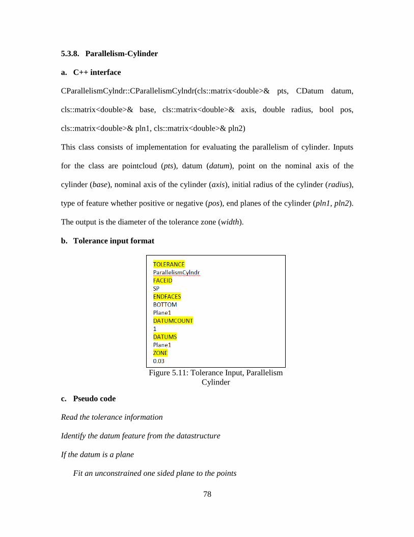
78

Parallelism-Cylinder 5.3.8.

a. C++ interface

CParallelismCylndr::CParallelismCylndr(cls::matrix<double>& pts, CDatum datum,

cls::matrix<double>& base, cls::matrix<double>& axis, double radius, bool pos,

cls::matrix<double>& pln1, cls::matrix<double>& pln2)

This class consists of implementation for evaluating the parallelism of cylinder. Inputs

for the class are pointcloud (pts), datum (datum), point on the nominal axis of the

cylinder (base), nominal axis of the cylinder (axis), initial radius of the cylinder (radius),

type of feature whether positive or negative (pos), end planes of the cylinder (pln1, pln2).

The output is the diameter of the tolerance zone (width).


c. Pseudo code





Figure 5.11: Tolerance Input, Parallelism

Cylinder

79

Identify the target feature and end planes from the datastructure and fetch the

information

Instantiate the CParallelismCylndr class with the feature and datum information

If the target feature is a hole fit an unconstrained maximum inscribed cylinder

Else fit an unconstrained minimum circumscribed cylinder to the pin

Calculate the intersection points of the axis with the end planes

Find the distances of these points from datum plane

The difference between these distances gives the parallelism error.

Perpendicularity-Plane: 5.3.9.

a. C++ interface

CPerpendicularityPlane(cls::matrix<double>& pts, CDatum datum)

This class implements the code for evaluating the perpendicularity of plane. Inputs for the

class are pointcloud (pts) and datum (datum). The output of the function is the width of

the tolerance zone.


c. Pseudo code



Perpendicularity Plane

80




If the datum is a hole

Fit an unconstrained maximum inscribed cylinder to the points

If the datum is a pin

Fit an unconstrained minimum circumscribed cylinder to the points

Identify the target feature from the datastructure and fetch the information

Instantiate the CPerpendicularityPln class with the feature and datum information

If the datum is plane

Fit a constrained minimum zone plane fit to the points on target feature

The width of zone gives perpendicularity error

If the datum is cylinder

Find the farthest and nearest points to the basepoint on the axis of datum, measured

along the direction of axis

The difference between the two distances gives perpendicularity error

Perpendicularity-Cylinder: 5.3.10.

a. C++ interface

CPerpendicularityCylndr(cls::matrix<double>& pts, CDatum datum,



This class implements the code for evaluating the perpendicularity of the cylinder. The

inputs required for this class are pointcloud (pts), datum (datum), point on the nominal

81

axis of the cylinder (base), nominal axis of the cylinder (axis), initial radius of the

cylinder (radius), type of feature whether positive or negative (pos), end planes of the

cylinder (pln1, pln2). The output is the diameter of the tolerance zone (width).


c. Pseudo code



Fit an unconstrained one sided plane to the points on the datum plane


information

Instantiate the CPerpendicularityCylndr class with the feature and datum information


Else fit an unconstrained minimum circumscribed cylinder

Calculate the intersection points of the axis with the end planes

Find the projection of these points on to the datum plane

The distance between the projected points gives the perpendicularity error.


Perpendicularity Cylinder

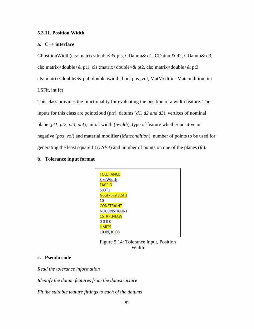
82

Position Width 5.3.11.

a. C++ interface

CPositionWidth(cls::matrix<double>& pts, CDatum& d1, CDatum& d2, CDatum& d3,

cls::matrix<double>& pt1, cls::matrix<double>& pt2, cls::matrix<double>& pt3,

cls::matrix<double>& pt4, double iwidth, bool pos_vol, MatModifier Matcondition, int

LSFit, int fc)

This class provides the functionality for evaluating the position of a width feature. The

inputs for this class are pointcloud (pts), datums (d1, d2 and d3), vertices of nominal

plane (pt1, pt2, pt3, pt4), initial width (iwidth), type of feature whether positive or

negative (pos_vol) and material modifier (Matcondition), number of points to be used for

generating the least square fit (LSFit) and number of points on one of the planes (fc).


c. Pseudo code


Identify the datum features from the datastructure

Fit the suitable feature fittings to each of the datums

Figure 5.14: Tolerance Input, Position

Width

83


information

Instantiate the CPositionWidth class with the feature and datum information

If the target feature is a slot fit an unconstrained internal minimum zone fit to the

points

Else fit an unconstrained external minimum zone fit to the points

For the mid-plane obtained from these fittings calculate the distances of its vertices

from the nominal plane

The position tolerance is equal to twice the maximum of these distances

Position Cylinder 5.3.12.

a. C++ interface

This is the child class of CPosition class providing the full functionality for evaluating the

position of a cylinder. The functional interface for this class is:

CPositionClndr(cls::matrix<double>& pts, CDatum& d1, CDatum& d2, CDatum& d3,

cls::matrix<double>& pln1, cls::matrix<double>& pln2, cls::matrix<double>& naxis,

cls::matrix<double>& npoint, double iradius, bool pos_vol, MatModifier Matcondition)

The inputs for this class are pointcloud (pts), datums (d1, d2 and d3), end planes of

cylinder (pln1, pln2), nominal axis of the cylinder (naxis), point on the nominal axis

(npoint), initial radius (iradius), type of feature whether positive or negative (pos_vol)

and material modifier (Matcondition). There are different combinations of datum

reference frames that can be applied to a position tolerance. But because of the number

and type of constraints that can be evaluated using the feature fitting library, only the

plane-plane-plane and plane-cylinder-slot/tab are implemented.

84


c. Pseudo code



Fit the suitable feature fittings to each of the datums


information

Instantiate the CPositionCylndr class with the feature and datum information


Else fit an unconstrained minimum circumscribed cylinder

Figure 5.15: Tolerance Input, Position

Cylinder

85

Find the intersection points of the axis with the end planes

Calculate the distances of these intersection points from the nominal axis

The position tolerance is equal to twice the maximum of these distances

Circular Runout 5.3.13.

a. C++ interface

CRunoutCircular(cls::matrix<double>& pts, CDatum& d1, CDatum& d2, int nlines, int*

pcount)

This class implements the functionality for evaluating the circular runout of a surface.

The inputs required for evaluating circular runout are pointcloud (pts), datums (d1, d2),

number of cross sections at which measurements are made (nlines) and a number of

points measured at each cross section (pcount). The output is the width of the tolerance

zone (width).


c. Pseudo code



Figure 5.16: Tolerance Input, Runout

Circular

86

Fit appropriate datums to the features

Identify the target feature from the datastructure

Instantiate the CRunoutCircular class with the feature and datum information

For each section of the target feature

Find the perpendicular distance between datum axis for each point

Find the maximum and minimum of these distances

The difference between these two gives the circular runout for that section

The maximum value of the runout among all the sections is the runout error for the target

feature

Total Runout 5.3.14.

a. C++ interface

CRunoutTotal(cls::matrix<double>& pts, CDatum& d1, CDatum& d2)

This class implements the functionality for evaluating the total runout of a surface. The

inputs required for evaluating circular runout are pointcloud (pts), datums (d1, d2). The

output is the width of the tolerance zone.


Figure 5.17: Tolerance Input, Runout

Total

87

c. Pseudo code



Fit appropriate datums to the features

Identify the target feature from the datastructure

Instantiate the CRunoutTotal class with the feature and datum information

Find the perpendicular distance between datum axis for each point

Find the maximum and minimum of these distances

The difference between these two gives the total runout for the feature.

88

CHAPTER 6

VALIDATION AND VERIFICATION

In this chapter the validation of the proposed algorithms is presented. The validation is

done by comparing the results obtained from the software with that of manual

measurements. To validate the proposed algorithms a sample of parts with known

variations are created. The parts are modeled with various types of geometric errors like

bowness, multiple lobes, surface waviness etc. so that they will be suitable for verifying

different tolerance types. The parts are modeled with possibly large values of errors so

Part 1

Part 2

Part 3 & 4

Figure 6.1: (a) Part 1, (b) Part 2, (c) Part 3 & Part 4

Part 3

89

Part 5 Part 6

Figure 6.2: (a) Part 5, (b) Part 6

that the errors caused by other factors will become negligible. The other factors that

influence the errors are angle of contact of CMM probe, diameter of CMM probe and the

errors caused in machining. The parts are shown in Figure 6.1 & Figure 6.2.

Part 1(Figure 6.1a) is a cylindrical pin modeled to measure size and form variations. Part

2 (Figure 6.1b) is modeled to measure flatness variations and also width variations. Part 3

(Figure 6.1c) is modeled to measure width variations and Part 4 (Figure 6.1c) is modeled

to measure form (circularity and cylindricity) variations. Part 5 is modeled to measure

orientation tolerances. The algorithms are verified based on the points measured on these

parts.

6.1. Size Verification

Size verification involves the verification of diameter or width of the features. So the

verification can be broadly classified into two categories- diameter verification and width

verification.

To verify diameter, Part 1 and Part 5 are used. Points are measured that are spread over

the surface of the work pieces. Then the points are taken as input and one sided fits are fit

to these points. The values of size obtained from the normative algorithms are: 20.12,

90

20.46. These values are validated by comparing them to the manual measurements. In

manual inspection size is measured at different cross sections of these parts. Then the

maximum value obtained between these is taken as the representative size of this part.

The sizes thus obtained from the manual inspections for part 1 and part 5 are 20.10,

20.43. These values are in comparison to that obtained from the software.

Verification of width is done using part 3 and part 4. Part 3 has a tab and part 4 has slot.

The sides of the tab and slot are modeled with considerable form errors in the order of

millimeters. Points are measured on each of the plane on each slot and tab. Then a

minimum zone fit is fit to these points. The value of size obtained from the fit is 20.87 for

tab and 19.07 for slot. Also the size is measured manually using precision parallels and

dial indicator. The value of size obtained is 20.87 for tab and 19.05 for slot.

6.2. Form Verification

In form verification, all the four types – straightness, flatness, circularity, cylindricity are

evaluated. Circularity and cylindricity are evaluated using Part 5. Part 5 is modeled with

form errors along the circumference with five lobes. The value of circularity obtained

from manual and normative procedures is 0.85 and 0.82. And the value of cylindricity is

0.85 from manual measurements and 0.82 from normative procedures.

Straightness and flatness are evaluated using Part 2. One of the faces of Part 2 is modeled

with surface waviness as the form error. Straightness is measured along four lines on the

surface using both the manual measurements and normative algorithms. The

corresponding values of straightness are 2.08 and 2.12. Also the flatness is measured

along the surface. The values of flatness obtained from manual measurements and

91

(a) (b)

Figure 6.3: Manual Inspection of Parts 2 & 5. (a) Flatness and

Straightness Measurements (b) Circularity, Cylindricity and Size

Verification

normative algorithms are 3.137 and 3.117. The manual measurements are taken using a

dial indicator, V-block and surface gauge [Figure 6.3].

6.3. Orientation Verification

In orientation, parallelism and perpendicularity are verified. Part 6 is used for the

verification of these. The “target face” in the figure is machined with surface variations

of known magnitude. The perpendicularity and parallelism variations of this “target face”

are evaluated with respect to the faces “Datum A” and “Datum B”. Parallelism is

evaluated between the “target face” and “Datum B”. The values of parallelism obtained

from manual measurements and normative algorithms are 18.71 and 18.84 respectively.

92

Perpendicularity is evaluated between “target face” and “Datum A”. The values of

perpendicularity obtained from manual measurements and normative algorithms are 3.89

and 3.97. In manual inspection the tolerances are evaluated using dial indicator, height

gauge and surface plate [Figure 6.5].

6.4. Position Verification

The position is verified using Part 6. Part 6 is modeled with a pin referred to three planar

datums. The part is modeled such that the pin has an initial orientation to the normal of

the primary datum. And the datums are modeled without any errors.

Figure 6.4: Datum and Target Faces in Part 5

Figure 6.5: Manual Inspection of Part 6

93

6.5. Runout Verification

Runout is verified using part 1. Part 1 has a perfect cylinder on some portion of the

length. And the other portion has variations. By taking the perfect part as the datum and

then measuring the variations on the other portion the runout tolerance can be verified.

The values of the runout obtained from the manual measurement methods and normative

procedures are 2.76 and 2.79.

In the above verification the values from manual inspection are in comparison with that

of the normative procedures. And as discussed in Section 4.1, both the GD&T standard

and manual inspection practices evolved together. So the confirmation of normative

procedures to the manual inspection methods shows the validity of normative procedures.

6.6. Case Study – Cylinder Cap

The verifications provided in the previous sections are evaluated separately. But the

software can evaluate multiple features in a part in a single instance. To demonstrate this

Figure 6.6: Cylinder Cap

94

capability the part shown in the Figure 6.6 is evaluated for position tolerance. In the

process the form and orientation tolerances of the datum features are also evaluated.

The part shown in the figure is the cap of a hydraulic cylinder. The part is fully

toleranced to meet the functional needs. The features that are functionally important are

the boss (SP in Figure 6.6), slot (slot), planar face (Plane 1) and the three holes (Hole1,

Hole2 and Hole3). Figure 6.7 shows the part with applied tolerances.

Points are measured on the functional features using a CMM. The points along with the

initial estimates are collected into a text file Cylinder_Cap.txt, in the format explained in

section 5.2. The tolerance information is also written to another text file Tolerances.txt.

The tolerances are evaluated using the developed software and the results are written to

the file Output.txt. Table 6.1 shows the results for this part.

Figure 6.7: Cylinder Cap, GD&T

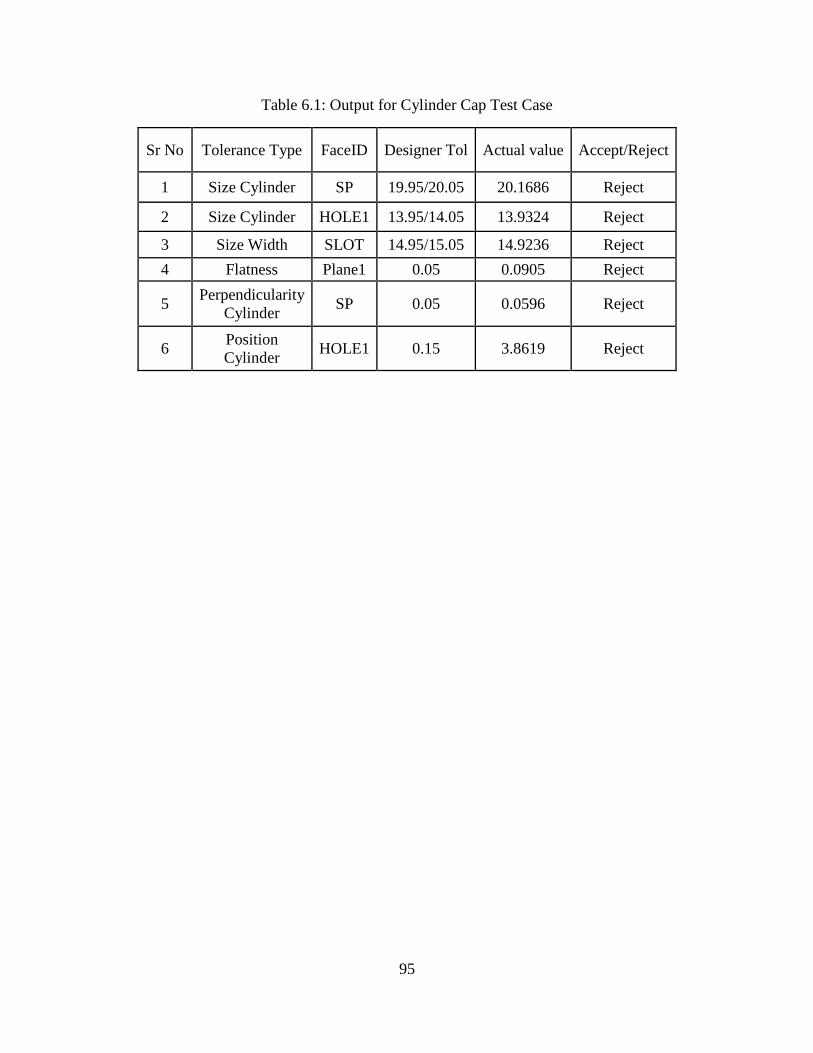
95

Table 6.1: Output for Cylinder Cap Test Case

Sr No Tolerance Type FaceID Designer Tol Actual value Accept/Reject

1 Size Cylinder SP 19.95/20.05 20.1686 Reject

2 Size Cylinder HOLE1 13.95/14.05 13.9324 Reject

3 Size Width SLOT 14.95/15.05 14.9236 Reject

4 Flatness Plane1 0.05 0.0905 Reject

5 Perpendicularity

Cylinder SP 0.05 0.0596 Reject

6 Position

Cylinder HOLE1 0.15 3.8619 Reject

96

CHAPTER 7

CONCLUSIONS

7.1. Normative Procedures

The commercial software in CMMs provides the user with different types of feature

fitting algorithms for evaluating tolerances. But using different types of feature fitting

algorithms for evaluating the tolerance on same feature gives different results. The type

of algorithm to be used is left to the discretion of the user. And there is no standard that

prescribes the type of feature fitting algorithms to be used for evaluating tolerances in

CMMs. To address these problems, normative procedures are proposed in this research.

These procedures are based on the standard definitions for tolerances and the manual

inspection practices used in the shop floor for measuring these tolerances. For proposing

the normative procedures, the standard definitions for each tolerance are interpreted to

understand the type of feature fitting that fits the definition. Then the manual inspection

practices are interpreted for understanding the type of feature fitting to be used. Then

both the interpretations are compared to decide on the type of feature fitting to be used

for evaluating the tolerances. During these interpretations it was found that some of the

manual inspection practices are not in agreement with the standard definitions. In such

cases, the criterions that dictate the assembly of features are used for deciding the

algorithms. Following this approach normative procedures are proposed for size, form,

orientation, position, runout and profile tolerances applied to line, plane, circle, cylinder

and width features. Some of these normative procedures are straightforward and the use

of feature fittings directly results in the geometric errors on the feature. But for some,

these results need to be further processed to obtain the geometric errors.

97

7.2. Software

The proposed normative procedures are implemented as software in C++. The feature

fitting library given in Table 2.1 is the base for implementing this software. It has all the

feature fitting algorithms required for implementing the normative procedures assorted

into a single place. The software functions by taking in the feature and tolerance

information from a text file and passing it to these algorithms. The results from these

algorithms are further processed if required for tolerance verification. Then the end

results of tolerance verification are written to a text file.

The software is object oriented and has the advantage that the user can evaluate the

tolerances of an entire part at one go. The same dataset for a feature can be used to

evaluate different tolerances on the feature. The sections below give the implementation

details of the software for different tolerances.

Size:

Normative procedures are proposed for verification of size on cylindrical and width

features. Constrained one sided fits are used for verification of size on datum features and

unconstrained one sided fits are used on the other features for evaluation of size.

Form:

Normative procedures for verification of straightness, flatness, circularity and cylindricity

are proposed. For straightness, unconstrained minimum zone line fits are used, for

flatness, unconstrained minimum zone plane fits are used, for circularity unconstrained

minimum zone circle fits are used and for cylindricity, unconstrained minimum zone

cylinder fits are used. Straightness and circularity are measured at multiple sections and

then the maximum value is taken as the corresponding form error.

98

Orientation:

In orientation, normative procedures for parallelism, perpendicularity and angularity are

proposed. In the case of planar features, constrained two sided fits are used for all of the

orientation tolerances. The width of the two sided fits gives the orientation error for

planar features. And for cylindrical features unconstrained one sided fits are used.

Position:

Position tolerances are evaluated by using unconstrained one sided fits. The axis/mid-

plane obtained from these fits, along with the datums, is used in calculating the positional

error of the feature.

Runout:

The normative procedures for runout tolerances do not need any feature fitting on the

target features. Instead of fitting a feature to the point cloud of the target feature, the

distances of these points from the datum axis are calculated and used for finding the

runout error. This helps save a lot of computation that goes into the feature fitting.

Profile:

Profile tolerances control size, form, orientation and position of a feature. Depending on

the type of control exercised by the profile, the normative procedures corresponding to

that tolerance control can be used.

7.3. Validation

To propose normative procedures the standard and the manual inspection practices are

compared with each other. Then suitable procedures are proposed for evaluating the

tolerances in CMMs. So to validate these procedures, the results from these procedures

are compared with manual inspection practices. Most of the results from the normative

99

procedures are in agreement with the manual inspection practices. For the results that are

not in agreement, the manual inspection practices differ from the standard definitions. A

case study is also presented to establish the usability of the software.

7.4. Future Work

In size verification, it is proposed to verify actual local sizes manually because of the

limitations in CMMs. If the CMMs can measure diametrically opposite points in future,

then the procedure for size verification has to be modified. Normative procedures for

coaxial features, pattern features, profiles other than circles and cylinders are not

proposed in this research. They can be developed in future. The feature fitting library

does not have algorithms that take angular constraints. So the normative procedures for

evaluating angular tolerances are not implemented. They can be developed in future if the

feature fitting library is extended. The software can be improved to have graphical output

of the data and feature fittings. Many of the feature fitting algorithms require initial

estimates of the feature. This can be automated by integrating the software with

geometric kernels like ACIS and then calculating the initial estimates from a CAD file.

100

REFERENCES

[1] American National Standard ASME Y14.5M. (2009). Dimensioning and Tolerancing,

The American Society of Mechanical Engineers, NY.

[2] American National Standard ASME Y14.5M. (1994). Dimensioning and

Tolerancing, The American Society of Mechanical Engineers, NY.

[3] Gary K Griffith, Geometric Dimensioning and Tolerancing Applications and

Inspection, second edition, Prentice Hall, 2001.

[4] ASME Y14.5.1, 1994, Mathematical Definition of Dimensioning and Tolerancing

Principles, The American Society of Mechanical Engineers, NY.

[5] T H Hopp, Computational Metrology Vol. 6, No. 4, Manufacturing Review,

American Society of Mechanical Engineers, New York (1993) pp 295-304.

[6] Stigler, S. M., 1990, The History of Statistics: The Measurement of Uncertainty

Before 1900, Belknap Press of Harvard University Press, Cambridge, MA.

[7] Vijay Srinivasan, Craig M Shakarji, Edward P Morse, On an Enduring Appeal of

Least Squares Fitting in Computational Metrology, Journal of Computing and

Information Science in Engineering, March 2012, Volume 12.

[8] Shakarji CM, Srinivasan V, (2012). Fitting weighted total least-squares planes and

parallel planes to support tolerancing Standards. CD-Rom Proceedings of the 32nd

ASME Computer and Information in Engineering Conf. Chicago, IL, August 12-15.

[9] Lipman Y, Cohen-Or D and Levin D. Error bounds and optimal neighborhoods for

MSL approximation. Proceedings of the 4th Eurographics symposium on Geometry

processing 2006;71-80.

[10] Polini W, Prisco U, Giorleo G. A new Algorithm to Assess Revolute Surface

through Theory of Surface Continuous Symmetry. In Models for Computer-Aided

Tolerancing in Design and Manufacturing (ed. J. K. Davidson), (Proc., 9th CIRP

Int'l Seminar on CAT, April 10-12, 2005, Tempe, AZ, USA). Springer, Dordrecht,

Netherlands;2007:157-166.

[11] Davidson, J.K., Savaliya, S.B., He, Y., and Shah, J.J., (2012). Methods of robotics

and the pseudoinverse to obtain the least-squares fit of measured points on line-

profiles. CD-Rom Proceedings of the 17th ASME Design for Mfg. and the Life

Cycle Conf. Chicago, IL, August 12-15.

101

[12] T.S.R. Murthy, S.Z. Abdin, Minimum zone evaluation of surfaces,

International Journal of Machine Tool Design and Research, 1979, Volume 20,

Issue 2, Pages 123-136

[13] Tohru Kanada, Soichiroh Suzuki, Evaluation of minimum zone flatness by means

of nonlinear optimization techniques and its verification, Precision Engineering,

1993, Volume 15, Issue 2, Pages 93-99.

[14] J. Meijer, W. de Bruin, Determination of flatness from straightness measurements

and characterization of the surface by four parameters, Precision Engineering, 1981,

Volume 3, Issue 1, Pages 17-22.

[15] Carr K, Ferreira P, Verification of form tolerances, part II: cylindricity and

straightness of a median line, Precision Engineering, 17(2), 1995, pp. 144-56.

[16] Choi W, Kurfess TR. Dimensional measurement data analysis, part 1: A zone fitting

algorithm. J Manuf Sci Eng 1999;121:238-45.

[17] Choi W, Kurfess TR. Dimensional measurement data analysis, part 2: Minimum

zone evaluation. J. Manuf. Sci. Eng 1999;121:246-50.

[18] Alistair B Forbes, 1991 (Revised Edition), Least Squares Best Fit Geometric

Elements, NPL Report DITC140/89, 1991.

[19] Craig M. Shakarji, Least Squares Fitting Algorithms of the NIST Algorithm Testing

System, Journal of research of the National Institute of Standards and Technology,

103(6), 1998.

[20] Craig M. Shakarji, Reference Algorithm for Chebyshev and One-Sided Data Fitting

for Coordinate Meteorology, CIRP Annals –Manufacturing Technology, 53(1), pp.

439-442, 2004.

[21] G.T. Anthony, H.M. Anthony, B. Bittner, B.P. Butler, M.G.Cox, R. Drieschner, R.

Elligsen, A.B. Forbes, H. Gross, S.A. Hannaby, P.M. Harris, J. Kok, Reference

software for finding Chebyshev best-fit geometric elements, Precision Engineering,

Volume 19, Issue 1, July 1996, Pages 28–36.

[22] Prashant Mohan, Development and verification of a library of feature fitting

algorithms for CMMs, Design Automation Lab, Master’s Thesis, 2014.

[23] Davidson J.K, Shah J.J. (2002), Goemtric tolerances: a new application for line

geometry and screws, IMechE J. of Mechanical Eng. Science, Part C;216:95-104.

102

[24] Robert J Hocken, Paulo H Pereira, Coordinate measuring machines and systems,

Second Edition, CRC Press, 2011.

[25] ANSI B89.3.1-1972 (R2003), Measurement of Out-of-Roundness.

[26] IMTI, A Roadmap for Metrology Interoperability (Integrated Manufacturing

Technology Initiative IMTI, Inc (2006).

103

APPENDIX-A

C++ SUBROUTINES FOR THE SOFTWARE

104

Size:

CSize: CSizeWidth, CSizeCircle, CSizeCylinder

CSizeWidth: This class has the implementations for finding the size of slot and tabs. Both

constrained and unconstrained versions are implemented. The constraints applicable are

parallel and perpendicular. The constructor for this class with all the inputs is given

below.

CSizeWidth(cls::matrix<double>& inpoints, bool pin_tab, Constraint cstr,

cls::matrix<double>& vec, int N1, int N2, int N3)

The inputs required are points measured on the surface (inpoints), information about the

feature- whether it is a pin or a tab (pin_tab), type of constraint (cstr), constraint direction

(vec), number of points required for generating the least square fit (N1), number of points

on each plane (N2, N3). The output is the width of tab or slot.

CSizeCircle: This class has the implementation for finding the size of circles. The

constructor for this class is given below.

CSizeCircle::CSizeCircle(cls::matrix<double>& points, bool pin_tab, Constraint cstr,

cls::matrix<double>& vec)

The inputs required for this class are the points measured on the circle (points),

information about the feature- whether pin or hole (pin_tab), type of constraint (cstr) and

the constraint direction (vec).

CSizeCylinder: The normative procedure for finding the size of a cylinder is

implemented in this class. The class has implementation for both constrained and

unconstrained versions. The constraints

applicable to this class are parallel and perpendicular. The constructor for this class is:

105

CSizeCylinder(cls::matrix<double>& points, bool pin_tab, Constraint cstr,

cls::matrix<double>& vec, cls::matrix<double>& axis, cls::matrix<double>& point,

double R)

The inputs required are points measured on the surface (points), information about the

feature – whether pin or hole (pin_tab), type of constraint (cstr), constraint direction

(vec), initial estimate of the direction of the axis (axis), initial estimate of the point on the

axis (point) and initial estimate of radius (R).

Form:

CForm: CFormStraightness, CFormFlatness, CFormCylindricity, CFormCircularity

CFormStraightness: This is a base class for straightness tolerance. It is an abstract class.

The algorithms for finding the straightness are different for planar and cylindrical

features. So two classes CStraightnessPlane, CStraightnessAxis are derived from this

class which contain the implementations for planar and cylindrical features respectively.

CStraightnessPlane: This class is derived from CFormStraightness. The algorithm for

defining straightness of a planar surface is defined in this class. The constructor for this

class is defined below:

CStraightnessPlane(cls::matrix<double>& pts, bool pin_tab, int nlines, int* pcount,

cls::matrix<double> RefPts)

The input required for this function are points measured on the surface (pts), feature type

– whether pin or tab (pin_tab), number of cross sections or lines (nlines), number of

points on each line (pcount) and points on the reference plane (RefPts). The output is the

width of the form zone.

106

CStraightnessAxis: This class is also derived from CFormStraightness. This class

consists of normative algorithm for evaluating straightness of axis. The constructor for

this class is

CStraightnessAxis(cls::matrix<double>& pts, bool pin_tab, int nlines, int* pcount,

cls::matrix<double> RefPts).

The input required for the function are points measured on the surface (pts), feature type

(pin_tab), number of lines (nlines), number of points in each line (pcount) and reference

point (RefPts). The output is the error of straightness on axis.

CFormFlatness:This class has the implementation for finding the flatness of a given

plane. The constructor for this class is defined below:

CFormFlatness(cls::matrix<double>& pts, int LSFit, int Total)

The inputs for this function are points measured on the surface (pts), number of points to

be used for least square fit (LSFit) and total number of points measured (Total). The

output is the width of zone

CFormCylindricity: This class contains implementation for finding the cylindricity of a

cylinder. The constructor for this class is:

CFormCylindricity(cls::matrix<double>& pts, cls::matrix<double> axis,

cls::matrix<double> basepoint, double R)

The inputs required for this function are points measured on surface (pts), initial estimate

of the axis of the cylindrical zone (axis), initial estimate of a point on the axis (basepoint)

and initial estimate of the radius (R). The output is the width of the zone.

CFormCircularity: This class is defined to evaluate the circularity errors on a cylinder.

The functional interface for initializing the class with the required inputs is given below.

107

CFormCircularity(cls::matrix<double>& pts, bool pin_tab, int nlines, int* pcount,

cls::matrix<double>& RefPts)

The inputs required for the evaluation of circularity are: points measured on the circular

cross-sections (pts), feature type whether pin or hole (pin_tab), number of cross sections

at which the measurements are made (nlines), number of points measured at each cross

section (pcount) and the points on the reference plane cloud (RefPts). The output is the

width of the zone that is maximum of all the sections.

Orientation:

COrientation: CParallelismPlane, CParallelismCylndr, CPerpendicularityPln,

CPerpendicularityCylndr

COrientation: COrientation is an abstract class for evaluating parallelism. The classes for

evaluating parallelism and perpendicularity of different types of features are derived from

this class. The child classes are defined below:

CParallelismPlane: This class consists of implementation for evaluating parallelism of a

plane. The functional interface for this class is:

CParallelismPlane::CParallelismPlane(cls::matrix<double>& pts, CDatum datum)

Inputs for the class are pointcloud (pts), datum information (datum) and the output is

width of the zone.

CParallelismCylndr: This class consists of implementation for evaluating the parallelism

of cylinder. The functional interface for instantiating this class is:

CParallelismCylndr::CParallelismCylndr(cls::matrix<double>& pts, CDatum datum,



108

Inputs for the class are pointcloud (pts), datum (datum), point on the nominal axis of the

cylinder (base), nominal axis of the cylinder (axis), initial radius of the cylinder (radius),

type of feature whether positive or negative (pos), end planes of the cylinder (pln1, pln2).

The output is the diameter of the tolerance zone (width).

CPerpendicularityPln: This class implements the code for evaluating the perpendicularity

of plane. The interface for this class is:

CPerpendicularityPlane(cls::matrix<double>& pts, CDatum datum)

Inputs for the class are pointcloud (pts) and datum (datum). The output of the function is

the width of the tolerance zone.

CPerpendicularityCylndr: This class implements the code for evaluating the

perpendicularity of the cylinder. The interface for declaring this class is:

CPerpendicularityCylndr(cls::matrix<double>& pts, CDatum datum,



The inputs required for this class are pointcloud (pts), datum (datum), point on the

nominal axis of the cylinder (base), nominal axis of the cylinder (axis), initial radius of

the cylinder (radius), type of feature whether positive or negative (pos), end planes of the

cylinder (pln1, pln2). The output is the diameter of the tolerance zone (width).

Position:

CPosition: CPosition is a base class providing the required member variables and the

functions for evaluating parallelism. This class only provides the basic structure and is

fully defined in child class. The child classes are CPositionSlotTab and

CPositionCylinder.

109

CPositionCylinder: This is the child class of CPosition class providing the full

functionality for evaluating the position of a cylinder. The functional interface for this

class is:

CPositionClndr(cls::matrix<double>& pts, CDatum& d1, CDatum& d2, CDatum& d3,

cls::matrix<double>& pln1, cls::matrix<double>& pln2, cls::matrix<double>& naxis,

cls::matrix<double>& npoint, double iradius, bool pos_vol, MatModifier Matcondition)

The inputs for this class are pointcloud (pts), datums (d1, d2 and d3), end planes of

cylinder (pln1, pln2), nominal axis of the cylinder (naxis), point on the nominal axis

(npoint), initial radius (iradius), type of feature whether positive or negative (pos_vol)

and material modifier (Matcondition).

Runout:

CRunOut: This is the base class of the implementation of runout tolerances. This class

defines the basic structure for the runout tolerances. The parameters and functions that

are common to either of the two circular runouts are declared in this class, but are not

fully defined. Their complete definitions are given in child classes CRunoutCircular and

CRunoutTotal derived from this base class.

CRunoutCircular: This class implements the functionality for evaluating the circular

runout of a surface. The functional interface for the class is:

CRunoutCircular(cls::matrix<double>& pts, CDatum& d1, CDatum& d2, int nlines, int*

pcount)

The inputs required for evaluating circular runout are pointcloud (pts), datums (d1, d2),

number of cross sections at which measurements are made (nlines) and a number of

110

points measured at each cross section (pcount). The output is the width of the tolerance

zone (width).

CRunoutTotal: This class implements the functionality for evaluating the total runout of a

surface. The functional interface for the class is:

CRunoutTotal(cls::matrix<double>& pts, CDatum& d1, CDatum& d2)

The inputs required for evaluating circular runout are pointcloud (pts), datums (d1, d2).

The output is the width of the tolerance zone.

reconciling the differences between tolerance … the differences between tolerance specification...

Documents