Recent sea level and upper ocean temperature variabilityand trends; cook islands regional results and perspective

D. E. Harrison & Mark Carson

Received: 12 January 2012 /Accepted: 27 August 2012 /Published online: 18 September 2012# U.S. Government 2012

Abstract The goal of this paper is to provide information on the sea level and upper oceantemperature variability and trends in the Cook Islands region within a global context. Oceanicfisheries variability and change take place within the physical environment. Because the state ofthe historical data set is not as would be desired, we begin with some review of data distributionissues. We provide some new results from the Cook Islands region but draw upon previouswork for information about the global and ocean-basin scale context. There are clear trends overrecent decades in sea level and, generally, in upper ocean temperature, but there is alsosubstantial interannual and interdecadal variability, which are larger locally than globally.Because of this variability, it is not possible to say if recent Cook Islands regional trends arerepresentative of longer-term trends, or if longer-term trends have increased recently. Trends inthe Cook Islands region over the last four decades are ~0.1–0.3 °C per decade in near surfacetemperature and ~2–3 cm sea level per decade.

1 Introduction

Oceanic fisheries are subject to variability and trends from many sources, which fisheriesmanagers and international treaty organizations seek to understand and respond to appro-priately. In the last few decades, concern about the possible effects of variability and trendsin the oceanic physical and chemical environment has risen (e.g., Mantua et al. 1997, Millerand Schneider 2000, Easterling et al. 2007). Increasing temperatures, sea level rise, areas ofanoxia, and ocean acidification are factors of interest, among others (e.g., Bindoff et al.2007). The need for summary level information appropriate to the fisheries community hasbeen identified. The Intergovernmental Panel on Climate Change (IPCC) Assessment

Climatic Change (2013) 119:37–48DOI 10.1007/s10584-012-0580-8

This article is part of the Special Issue on “Climate and Oceanic Fisheries” with Guest Editor James Salinger

D. E. Harrison (*)NOAA/PMEL and University of Washington, Seattle, WA, USAe-mail: d.e.harrison@noaa.gov

M. CarsonUniversity of Hamburg, KlimaCampus, Hamburg, Germany

Reports have focused on and summarized much useful global-scale information abouttrends, and oceanic variability is receiving increased attention. Unfortunately, the openocean marine environment has not been systematically and globally monitored, even fortemperature, salinity, and sea level, until quite recently (e.g., Harrison and Carson 2008).Thus it is challenging to construct reliable estimates of regional and local behavior in manyareas of limited observations. There even remain issues about how effectively long-termglobal averages can be computed with the historical data sets (e.g., Lyman and Johnson2008). Of particular interest, but also a particular challenge, is the detection of recentincreases in trends which might indicate a need for enhanced management activity.

The estimation of oceanic trends on fisheries must be considered in the context of oceanicvariability, which can be quite strong regionally and locally. The seasonal cycle of surfaceocean temperature can be several degrees celsius, even in the tropics (up to 5 °C, peak topeak in long-term sea surface temperature, (SST) climatologies), and over 10 °C in somewestern boundary current areas, with decreasing but substantial magnitude ( >5 °C) near themixed layer (not shown, cf. Locarini et al. 2006). The El Niño-Southern Oscillation (ENSO)involves interannual changes in upper ocean temperature of more than 4 °C in some regions,with sea level changes greater than 10 cm in many tropical areas. There can be alsosubstantial decadal variability. Harrison and Carson (2007, 2008) (and updated in Carsonand Harrison 2010) showed 20-year trends of near surface ocean temperatures, which rangeup to 2 °C (20 year)−1 across extensive regions. There are regions of warming and cooling inevery analysis we have performed, so estimates of the world ocean average are affected byhow interpolation is done across data-poor areas. Moreover, different 20-year trend periodsgenerally lead to regions that were cooling in one time period are found to be warming inanother. Decadal trends in local sea level can easily vary by several cm/decade.

Our ability to determine the characteristics of the variability and trends of oceanic sea level,temperature, and heat content is strongly affected by the historical distribution (and quality) ofobservations. Much effort has been devoted to estimating world-ocean-average upper oceanheat content trends, and early results from Levitus et al. (2000) compared well to detection andattribution model studies (Barnett et al. 2001). Subsequently, issues with the historical data sethave led to adjustments and some results have been revised downward (e.g., global ocean heatcontent by 5.5×1022J between Levitus et al. 2000 and Levitus et al. 2009). However, all studiesagree that there has been net upper ocean warming since the 1970s.

It is worthwhile to revisit the historical spatial distribution of oceanic temperatureobservations in a recent version of the World Ocean Atlas (WOA05, Locarini et al. 2006;Fig. 1). Figure 1 presents the total number of observations over the entire 150-year period,prior to deployment of the Argo drifting float array. Data coverage has increased substan-tially in the last decade since Argo was deployed, but for historical estimates, the figureillustrates many of the challenges. The deeper the depth of interest, the poorer the sampling.Overall, the Southern Hemisphere has been poorly sampled, but a surprising number ofNorthern Hemisphere regions also have not been well sampled. The majority of the oceanvolume has, over most of the historical record, not been sampled adequately for meaningfullocal or, often, regional long-term trend estimation.

Much attention has been given recently to estimates of global average sea level risebecause global climate model projections suggest that sea level rise will increase in comingdecades, and because sea level rise has been observed at most long-term tide gauge stations.While sea level change does not have the impact on fisheries that temperature and chemicalchanges do, it is important for low-lying islands and nearshore regions. Making centurytime-scale estimates of the rise in sea level is challenging because there are not many tidegauges with climate-useful records of this length and because the tide gauge network of

38 Climatic Change (2013) 119:37–48

suitable gauges has changed greatly over time (See Fig. 2). Various statistical approacheshave been used to try to extract the global scale signal from the tide gauge network, and thework of Church and White (e.g., Church et al. 2004; Church and White 2006) is widelyreferenced. They find that the average rate of increase over the last century has been +1.7±0.2 mmyr−1.

A major advance in knowledge of sea surface height (SSH) variability took place with theflight of the TOPEX/POSEIDON precision altimeter mission in 1992, which providednearly complete coverage of the ice-free world ocean, with repeat coverage after every21 days. This altimetric mission was followed by successor high-precision missions,JASON-1 and JASON-2, to produce a 20-year record. The precision-altimeter-mission-eratime series of mean sea level can be smoothed in various ways to reduce the substantialinterannual variability, but the full-record global trend is about 3 mmyr−1. This is in goodagreement with tide gauge estimates of global sea level rise over the same period (Churchand White 2011). Whether this represents an increase in the historical century-scale trend ormulti-decadal trend variability only will become clear in the future (particularly if precisionaltimeter missions continue to be flown).

There is very substantial spatial variation in the satellite-era trend (see Aviso, http://www.aviso.oceanobs.com/en/news/ocean-indicators/mean-sea-level/), with the greatestregional increases in the western tropical Pacific, where ENSO variability is strongand known to have a large decadal variability, (e.g., Lee and McPhaden 2008; Wangand Mehta 2008). Local observations are critical to provide accurate local sea levelrise information.

Fig. 1 Number of temperature observations in World Ocean Atlas 2005 (thus the counts are mostly prior toArgo) by 2°×2° regions, after Fig. 2 in Harrison and Carson (2007). Only regions with 10 or moreobservations are colored. Depth bins shown are: a 100; b 300; c 500; d 600; e 1000; and f 2000 m

Climatic Change (2013) 119:37–48 39

However, low-frequency variability is indistinguishable from a trend over data sets ofonly a few decades, yet the management response to cyclical temperature variability likelyought to be quite different to that from a long-term trend. Caution in the interpretation oftrends estimated from 20- to 30-year data sets seems very much in order, until longer datarecords are obtained and analyzed. We shall illustrate this with examples from the CookIslands region in Section 3.

Because regional observations show larger interannual and interdecadal variability thanbasin-scale or global averages, management decisions in local waters would be wise to focuson what has been observed locally and regionally. Local and regional variability will oftenhave larger consequences in the next few decades than will global change trends. Of courseit is important for regional managers also to keep an eye on the longer-term temperature andsea-level trends from climate model projections, and to see how well local conditions

Fig. 2 From Church and White (2011, their Fig. 1). Number of tide gauge locations available in the PSMSLarchive by hemisphere and year (a), and spatially by decade (b–f)

40 Climatic Change (2013) 119:37–48

compare with the projections. Hopefully the climate change models will be increasingly ableto provide useful information about the magnitude of local future trends. It is critical tosustain the enhanced ocean observing activities that have been undertaken over recentdecades if policy makers and managers are to have accurate local and regional informationto determine rates of local change, and against which to evaluate model projections.

2 Data and methods

To explore the variability and recent evolution of SSH and upper ocean temperature, bothglobally and in the vicinity of the Cook Islands, an assortment of data was used. For SSH,Aviso provides a merged satellite data product, which combines all altimetry data backthrough late 1992 with the advent of TOPEX / POSEIDON (Aviso, accessed Oct. 2010). Aversion of this satellite data is also provided by the Commonwealth Scientific and IndustrialResearch Organisation (CSIRO, http://www.cmar.csiro.au/sealevel; accessed Nov. 2011).Church and White (2011, CW11, data accessed July 2011) use this CSIRO data set ofglobal SSH observations to estimate large-scale variability using empirical orthogonalfunctions (EOFs), and with these loading patterns, extend the regional SSH record back intime by constraining the patterns to available tide gauge data. These two data sets are bothuseful to establish a global picture of SSH variability, although it is unclear how much theEOF-interpolated dataset captures the real historical SSH variability of the open ocean.

Tide gauges themselves are, of course, bound to land and are susceptible to a variety ofpotential biases, most of which are discussed in Church et al. (2004). Annual tide gauge dataare examined here for some stations around the Cook Islands, and were downloaded fromthe Permanent Service for Mean Sea Level (PSMSL 2011, www.psmsl.org, accessed March2011; Woodworth and Player 2003). There was no extra processing of the tide gauge data,the consequences of which are discussed under the Results section below.

The temperature and salinity data came from available historical temperature and salinityprofiles stored in the World Ocean Database 2009 (WOD09; Boyer et al. 2009). However, asnoted above, the data can be exceedingly sparse in regions prior to the Argo float era (i.e.,2004), so two data sets that use objective interpolation schemes to fill data gaps were alsoused: the Historical Ocean Subsurface Temperature Analysis, v. 6.7, Ishii and Kimoto (2009,Ish6.7); and the NODC Global Ocean Heat Content seasonal temperature anomaly fields,Levitus et al. (2009, LEV09). SST from HadISST v1.1 (Rayner et al. 2003) is also analyzed.

All datasets, except for the annual average PSMSL tide gauge data and one version of theCSIRO-processed satellite data, are either provided as monthly or seasonal anomalies (theseasonal cycle has been removed), or have climatologies estimated from their data andmonthly anomalies calculated. Seasonal variability was computed from the estimated cli-matologies, interdecadal variability from 10-year running means of the anomalies (using aHanning window for smoother results), and interannual variability from the monthlyanomalies minus the 10-year running mean.

3 Results

3.1 Sea level

Sea level rise is of great concern to low-lying islands and coastal areas, both on its own, andbecause positive trends increase the probability and severity of flooding events from severe

Climatic Change (2013) 119:37–48 41

weather. Ultimately, nations are interested in regional and local sea level rise, since it is thiswhich most strongly affects their interests. There is no substitute for climate-quality tidegauge records to provide local information. However, an accurate very long-term trend, orclimate change signal, in these records is seldom easily identified. As noted previously, thisis because, typically, there is sufficient interannual to decadal variability in individual tidegauge records to seriously alias longer-term trend estimates. Particularly in the developingworld, long climate-quality records are not available in many areas. Typically, at best, a fewdecades of data are available.

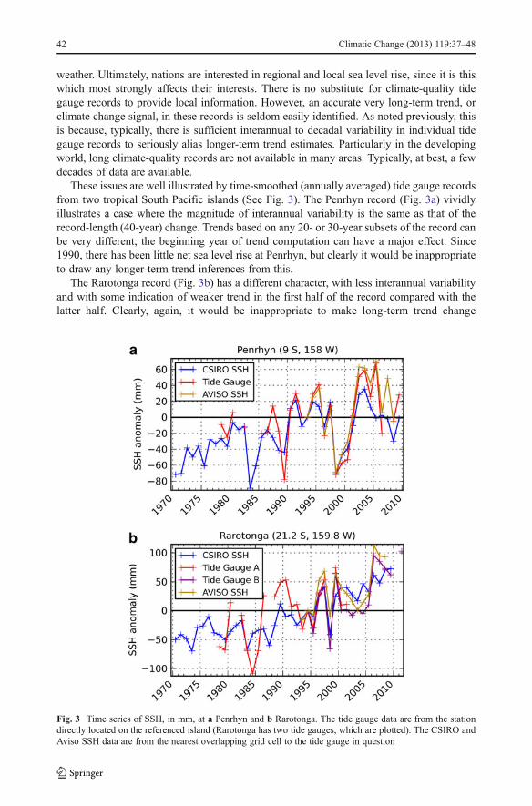
These issues are well illustrated by time-smoothed (annually averaged) tide gauge recordsfrom two tropical South Pacific islands (See Fig. 3). The Penrhyn record (Fig. 3a) vividlyillustrates a case where the magnitude of interannual variability is the same as that of therecord-length (40-year) change. Trends based on any 20- or 30-year subsets of the record canbe very different; the beginning year of trend computation can have a major effect. Since1990, there has been little net sea level rise at Penrhyn, but clearly it would be inappropriateto draw any longer-term trend inferences from this.

The Rarotonga record (Fig. 3b) has a different character, with less interannual variabilityand with some indication of weaker trend in the first half of the record compared with thelatter half. Clearly, again, it would be inappropriate to make long-term trend change

Fig. 3 Time series of SSH, in mm, at a Penrhyn and b Rarotonga. The tide gauge data are from the stationdirectly located on the referenced island (Rarotonga has two tide gauges, which are plotted). The CSIRO andAviso SSH data are from the nearest overlapping grid cell to the tide gauge in question

42 Climatic Change (2013) 119:37–48

inferences from this record. Despite their proximity, the very different behavior exhibitedillustrates the importance of local information for local decision-making.

Despite the difficulties of speaking to the absolute magnitude of sea level rise, it is clearthat these stations have experienced rising sea level over the period of their tide gaugerecords. A rough trend of ~2 mmyr−1 is evident at Penrhyn and of ~3 mmyr−1 at Rarotonga.If these trends persist, this sector of the South Pacific will experience a sea level rise of ~20–30 cm (~8–12 in) over the coming century. For CMIP3 projections using the Special Reporton Emission Scenarios A1B scenario, the local sea level change is projected to increase over40 cm by 2100, though with significant model spread (some project over 50 cm rise in thisregion of the Pacific by 2100; Slangen et al. 2012).

We can illustrate roughly the importance of climate variability by comparing it to both themagnitude of the seasonal cycle and the available trend estimates. We have used the 18 yearsof data from the satellite altimeter era to estimate regional seasonal and “interannual”variability variances (Fig. 4). (Note that the “interannual” variability here includes allvariability over periods longer than a year, since there is not enough satellite data to performa useful 10-year running mean low-pass filter with good temporal coverage, as is done withother data sets.) The variability on these shorter time scales is large for individual locations,with seasonal standard deviation of SSH of about 20 mm at Rarotonga, and about 24 mmnear Penrhyn (Fig. 4a). The interannual variability, on the other hand, is ~25–30 mm for thesouthern islands, and reaches 45 mm for the northern islands (Fig. 4b). The ratio ofinterannual to seasonal variability is above 1 for most of this entire region (Fig. 4c). Theinterannual variability to decadal trend ratio (Fig. 4d) is large nearer to the equator, and dropsto less than 1 for the southern Cook Islands.

This means that year-to-year changes can easily be larger than the longer-term trend inSSH in the north, and is comparable to it in the south. Even in the south year-to-yearfluctuations can be much larger than the longer-term trend (cf., e.g., the tide gauge datachanges between 2005 and 2006 in Fig. 3b). This means that in the short term (the next 10 to20 years) interannual variability is likely to provide a larger impact on low-lying islands thanthe change in sea level over the same period. But in the long term (century time scale) thepermanent change in sea level (if projections prove correct) will be a big concern, especiallygiven that interannual variability will be superimposed on a higher background sea levelstate.

3.2 Temperature/heat content

As mentioned above, long-term temperature change and variability can be an importantfactor to ecosystems and the fisheries industry as changing environment can lead to largeshifts in commercial fisheries locations as well as affecting local conditions (like coral reefecosystems). Since SST is better measured across this region than SSH (and subsurfacetemperatures too), an analysis of the variability on different time scales is more trustworthyfor this property (Fig. 5). We decompose the variance in the observations as described above,into seasonal, interannual, and decadal components, to illustrate the magnitude of climatevariability effects. The temperature variability for the southern Cook Islands is strongest onseasonal time scales, as the annual cycle is stronger in the subtropical gyre than along theequatorial band. The inverse is roughly true of interannual time scales, where the variabilityis strongest along the equator, although there is a minimum distinguishable between theequatorial band and the subtropical gyre. This pattern is similarly reproduced on longer timescales, where both the northern and southern Cook Islands are in the regions of strongerinterdecadal variability, with the band of weaker variability separating them (Fig. 5c).

Climatic Change (2013) 119:37–48 43

However, for the entire region, it appears that interdecadal variability is larger than thedecadal trend (Fig. 5d). Thus, at least for surface temperatures in the next few decades, thelong-term SST change factor is not as large an element in the local climate system as is thedecadal time scale variability.

Keeping in mind that the subsurface ocean has been poorly sampled over the course ofdecades, especially south of the equator, some local details of the subsurface timescales ofvariability nonetheless are shown in Fig. 6. The seasonal variability, stronger in the southernsubtropical gyre near the surface as seen above, decreases with depth in that region, whereasit increases to a subsurface maximum at the equator. Here it is focused along the

Fig. 4 SSH variability in the vicinity of the Cook Islands, from the CSIRO-gridded satellite altimetry data(1993–2011). No inverse barometer correction has been made, so that the full local impact of changing SSH isshown. (a) Seasonal variability, in mm; (b) interannual variability, from yearly averages of monthly anomalies,detrended, in mm; (c) ratio of interannual to seasonal variability; and (d) ratio of interannual variability to themagnitude of the decadal trend (i.e., in mm [10 year]−1). White blocks in the upper right portion of (d) arelocations where the SSH trend is nearly zero in the altimetry data

44 Climatic Change (2013) 119:37–48

thermocline, coincident with the equatorial countercurrent (not shown). The localmaximum for interdecadal variability is also located within the thermocline, and is alarge fraction of the seasonal variability in the vicinity of the thermocline, and belowit, from the equatorial band to the subtropical gyre (Fig. 6, lower panel). Schneider etal. (1999) found decadal anomalies propagating in the thermocline from the ventilatedregions poleward of the subtropical gyre toward the tropics in the North Pacific.Further reviews of mechanisms of decadal variability in the Pacific oceans betweenthe tropics and extratropics are presented in Liu and Alexander (2007). Regardless ofmechanism, a significant portion of the low-frequency thermosteric SSH changes inthis region are probably traceable to low-frequency temperature changes in and belowthe seasonal thermocline.

Fig. 5 SST variability from the HadISST1.1 for the Cook Islands region (1950–2009 period). a Seasonalvariability (°C); b interannual variability (from high-passed monthly anomalies, °C); c interdecadal variability(from low-passed monthly anomalies, 121-month Hanning window, °C); and d interdecadal variability todecadal trend ratio [decadal trend calculated as °C (10 year)−1 over the 1970–2009 period

Climatic Change (2013) 119:37–48 45

4 Summary and discussion

We have used observations from the Cook Island region to illustrate the challenges of tryingto identify very long-term (climate change) trends in our highly variable ocean environment.We have also used earlier published work to provide global context for perspective on theresults for the Cook Island region.

There are clear trends over the past 40 years in SST, upper ocean temperature, and sealevel in the Cook Island region. Sea level has been rising in the range of 2–3 cm/decade andtemperature has been increasing in the range of 0.1–0.3 °C/decade. Both sea level and upperocean temperature trends fall within the ranges estimated for recent global mean trends.However, there is sufficient interannual to decadal variability in the regional results toconfound efforts to determine if the rates of increase are increasing (or decreasing).

Due to the magnitude of climate variability, regional climate variability is likely to morestrongly influence the regional fisheries environment over the next few decades than will theclimate change signal. Only on the century time scale, based on present trends, will climatechange environmental signals come to clearly stand out compared with climate variability.Thus fishery managers in most regions should pay at least as much attention to climatevariability as to estimates of climate change over the coming decades. Policy makers areadvised to not overreact to the appearance of changes (increases or decreases) in local or

Fig. 6 Temperature section, in °C, along 150°W (the meridian along which WOCE section P16 is repeated).Seasonal variability is calculated as the standard deviation of the monthly climatology, and the decadalvariability as the standard deviation of the detrended 10-year running mean of monthly anomalies. The bottompanel shows the ratio of seasonal and decadal variability (the top left panel divided by the top right one)

46 Climatic Change (2013) 119:37–48

regional multi-year trends. We strongly encourage regional fisheries managers to understandthe magnitude of climate variability in the regions of concern to them.

There is a strong need for ongoing investment in local, regional, and global oceanobserving systems, particularly to identify local rates of change in environmental conditionsas well as to evaluate the plausibility of climate change model projections. Qualitativeknowledge of historical patterns of species biomass and recruitment variability meritconsideration as well. We must learn as much as we can about climate variability as wellas projections of climate change if wise decision-making is to take place in coming decades.

Acknowledgments This work was supported by the NOAA Office of Climate Observations and NOAA’sPacific Marine Environment Laboratory. “The altimeter products were produced by Ssalto/Duacs anddistributed by Aviso, with support from Cnes (http://www.aviso.oceanobs.com/duacs/).” The tide gauge datawas provided by the Permanent Service for Mean Sea Level.

References

Aviso. http://www.aviso.oceanobs.com. Accessed October 2010Barnett TP, Pierce DW, Schnur R (2001) Detection of anthropogenic climate change in the world’s oceans.

Science 292:270–274Bindoff NL, Willebrand J, Artale V, Cazenave A, Gregory J, Gulev S, Hanawa K, Le Quéré C, Levitus S,

Nojiri Y, Shum CK, Talley LD, Unnikrishnan A (2007) Observations: oceanic climate change and sealevel. Climate change 2007: the physical science basis. In: Solomon S, Qin D, Manning M, Chen Z,Marquis M, Averyt KB, Tignor M, Miller HL (eds) Contribution of working group I to the fourthassessment report of the intergovernmental panel on climate change. Cambridge University Press,Cambridge, pp 385–432

Boyer TP, et al (2009) World Ocean Database 2009. NOAA Atlas NESDIS 66, p 216Carson M, Harrison DE (2010) Regional interdecadal variability in bias-corrected ocean temperature data. J

Climate 23:2847–2855Church JA, White NJ (2006) A 20th century acceleration in global sea-level rise. Geophys Res Lett 33:

L01602. doi:10.1029/2005GL024826Church JA, White NJ (2011) Sea-level rise from the late 19th to the early 21st century. Surv Geophys 32:585–

602Church JA, White NJ, Coleman R, Lambeck K, Mitrovica JX (2004) Estimates of regional distribution of sea

level rise over the 1950–2000 period. J Climate 17:2609–2625Easterling WE, Aggarwal PK, Batima P, Brander KM, Erda L, Howden SM, Kirilenko A, Morton J, Soussana

JF, Schmidhuber J, Tubiello FN (2007) Food, fibre and forest products. Climate change 2007: impacts,adaptation and vulnerability. In: Parry ML, Canziani OF, Palutikof JP, van der Linden PJ, Hanson CE(eds) Contribution of working group II to the fourth assessment report of the intergovernmental panel onclimate change. Cambridge University Press, Cambridge, pp 273–313

Harrison DE, Carson M (2007) Is the world ocean warming? Upper-ocean temperature trends: 1950–2000. JPhys Oceanogr 37:174–187

Harrison DE, Carson M (2008) Upper ocean warming: Spatial patterns of trends and interdecadal variability.NOAA Tech Memo OAR PMEL-138, p 35 [Available online at http://www.pmel.noaa.gov/pubs/PDF/harr3144/harr3144.pdf]

Ishii M, Kimoto M (2009) Reevaluation of historical ocean heat content variations with time-varying XBTandMBT depth bias corrections. J Oceanogr 65:287–299

Lee T, McPhaden MJ (2008) Decadal phase change in the large-scale sea level and winds in the Indo-Pacificregion at the end of the 20th century. Geophys Res Lett 35:L01605. doi:10.1029/2007GL032419

Levitus S, Antonov JI, Boyer TP, Stephens C (2000) Warming of the World Ocean. Science287:2225–2229

Levitus S, Antonov JI, Boyer TP, Locarini RA, Garcia HE, Mishonov AV (2009) Global ocean heat content1955–2008 in light of recently revealed instrumentation problems. Geophys Res Lett 36:L07608.doi:10.1029/2008GL037115

Climatic Change (2013) 119:37–48 47

Liu Z, Alexander M (2007) Atmospheric bridge, oceanic tunnel, and global climatic teleconnections. RevGeophys 45:RG200, doi: 10.1029/2005RG000172

Locarini RA, Mishonov AV, Antonov JI, Boyer TP, Garcia HE (2006) Temperature. Vol 1, World Ocean Atlas2005, NOAA Atlas NESDIS 61, p 182

Lyman JM, Johnson GC (2008) Estimating annual global upper-ocean heat content anomalies despite irregularin situ ocean sampling. J Climate 21:5629–5641

Mantua NJ, Hare SR, Zhang Y, Wallace JM, Francis RC (1997) A Pacific interdecadal climate oscillation withimpacts on salmon production. Bull Amer Meteor Soc 78:1069–1079

Miller AJ, Schneider N (2000) Interdecadal climate regime dynamics in the North Pacific Ocean: theories,observations, and ecosystem impacts. Prog Oceanogr 47:355–379

Permanent Service for Mean Sea Level (PSMSL) (2011) “Tide Gauge Data” http://www.psmsl.org/data/obtaining/. Accessed 23 Mar 2011

Rayner NA, Parker DE, Horton EB, Folland CK, Alexander LV, Rowell DP, Kent EC, Kaplan A (2003)Global analyses of sea surface temperature, sea ice, and night marine air temperature since the latenineteenth century. J Geophys Res 108:4407. doi:10.1029/2002JD002670

Schneider N, Miller AJ, Alexander MA, Deser C (1999) Subduction of decadal North Pacific temperatureanomalies: observations and dynamics. J Phys Oceanogr 29:1056–1070

Slangen ABA, Katsman CA, van de Wal RSW, Vermeersen LLA, Riva REM (2012) Towards regionalprojections of twenty-first century sea-level change based on IPCC SRES scenarios. Clim Dyn38:1191–1209

Wang H, Mehta VM (2008) Decadal variability of the Indo-Pacific warm pool and its association withatmospheric and oceanic variability in the NCEP-NCAR and SODA reanalyses. J Climate 21:5545–5565

Woodworth PL, Player R (2003) The permanent service for mean sea level: an update to the 21st century. JCoastal Res 19:287–295

48 Climatic Change (2013) 119:37–48