recent progress in preliminary design of mechanical
TRANSCRIPT
OPTIMALITY CRITERIA
Pierre DUYSINX
LTAS – Automotive Engineering
Academic year 2020-2021
1

LAYOUT OF THE LESSON
Introduction & Motivation
Analysis using Principle of Virtual Work and Finite Element Method
Optimality criteria for fully stressed design
Berke’s approximation of displacement
Optimality criteria for a single displacement constraint
Optimality criteria for several displacement and stress constraints
2

INTRODUCTION & MOTIVATION
3
Introduction: Historical Context
▪ First developments: 1960 L. Schmit
▪ Extension of the approach carried out in economy, in chemical engineering, etc.
▪ Structural analysis: first Finite Element Models.
▪ Only simple elements: bars, shear panels, plates, beams, shells…
▪ Conquest of air and space: lightweight thin-wall structures
▪ Geometrical modelling, free mesh generation, sensitivity analysis, etc. are not yet developed
▪ Design variables are sizing variables attached to the F.E.
▪ Development of computers and their application to engineering
4
Introduction: Historical Context
▪ Mathematical Programming methods are under construction
▪ Unconstrained minimization → OK
▪ Linear programming (linear objective function subject to linear constraints) → OK
▪ Nonlinear programming: nonlinear objective function subject to nonlinear constraints → Under development in
the 1960ies
▪ Extension of optimization methods for linear constraints
▪ Strategy based on the following the active constraints
▪ Alternating minimization phases and restoring phases to come to feasible domain → projection methods
▪ Feasible direction methods
➔ Costly and so not applicable to engineering problems
because non explicit problems requires one FE analysis at each function evaluation 5
Introduction: Historical Context
▪ Focus on sizing problems of linear elastic structures with thin walls
▪ Design variables are the cross-sectional areas and plate thicknesses
▪ Typical problems: n-bar truss…
▪ Mass minimization
▪ Research for the development of fast convergence and reliable algorithms involving little novel concepts (apart from the sensitivity analysis)
▪ No additional development at F.E. level
▪ Design variables are properties of F.E. (fixed mesh, discrete variables)
6
Introduction: Historical Context
▪ Search for an alternative approach to Mathematical Programming methods, which are too costly.
▪ Optimization becomes a particular field concerned with aerospace and research.
7
Introduction: Mathematical Programming approach
▪ MP approach aims at solving structural optimization problems combining a general numerical optimization algorithm and a computer simulation code (e.g. FEM)
▪ Different approaches are possible
▪ Direct methods
▪ Projection methods
▪ Feasible direction (Zoutendijk)
▪ Reduced gradient
▪ Solution cost is proportional to the problem size
8

Introduction: Mathematical Programming approach
▪ Transformation methods:
▪ The solution cost of the transformed problem growths with its size.
▪ The number of transformed problems to build and solve depends on the quality (accuracy, precision…) of the transformation
▪ Two main groups of approaches
▪ Unconstrained minimization methods
▪ Methods based on approximations
9
Introduction: Mathematical Programming approach
▪ Transformation methods:
▪ Unconstrained minimization methods
▪ Interior penalty methods
▪ Exterior penalty methods
▪ Extended interior penalty methods
▪ Augmented Lagrangian method
▪ Methods based on approximations
▪ Linear Sequential Programming
▪ Quadratic Sequential Programming
▪ Sequential Convex Linearization (CONLIN, MMA…)
10
Introduction: Mathematical Programming approach
▪ In any cases,
▪ Mathematical Programming approach is generally reliable
▪ The sensitivity analysis is necessary because MP are based on the derivatives (at least first order derivatives, the gradients)
▪ Older methods are not applicable to structural optimization because of their poor performance
▪ Research since the 60ies
▪ Reduction of the cost of sensitivity analysis
▪ Automatic differentiation, iterative methods, approximate re-analysis
▪ Development of optimality criteria methods
▪ Development of approximation concepts11
Introduction: Optimality Criteria methods
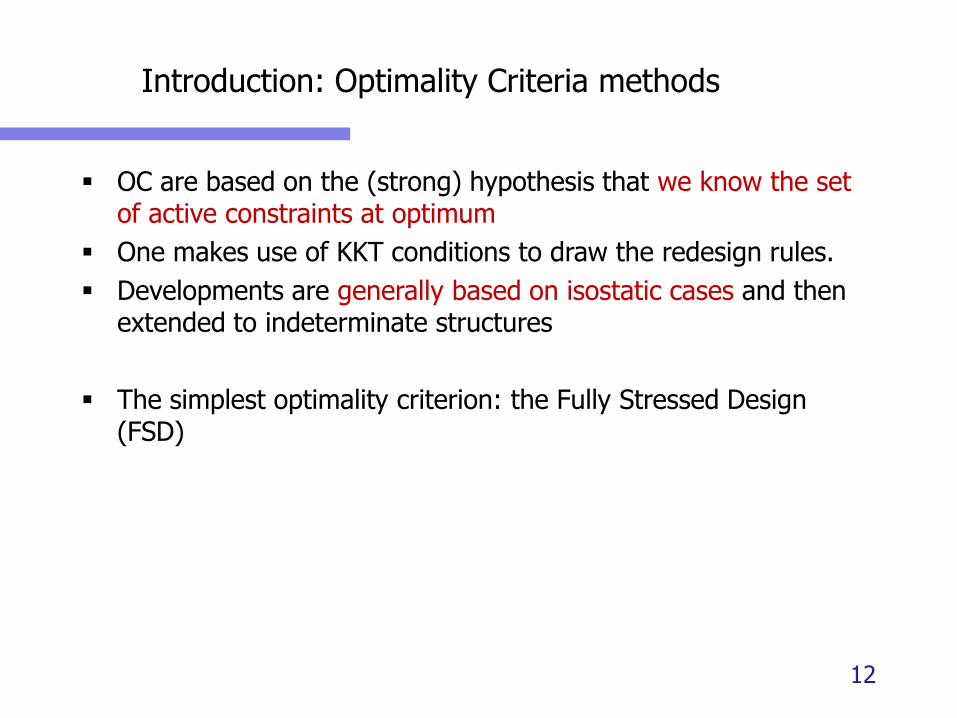
▪ OC are based on the (strong) hypothesis that we know the set of active constraints at optimum
▪ One makes use of KKT conditions to draw the redesign rules.
▪ Developments are generally based on isostatic cases and then extended to indeterminate structures
▪ The simplest optimality criterion: the Fully Stressed Design (FSD)
12
Introduction
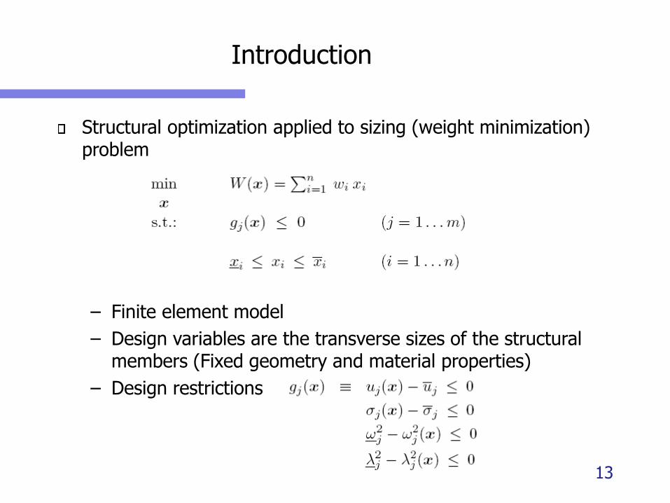
Structural optimization applied to sizing (weight minimization) problem
– Finite element model
– Design variables are the transverse sizes of the structural members (Fixed geometry and material properties)
– Design restrictions
13

Introduction
Design constraints gj(x)<0
– Implicit functions
– Nonlinear functions
– One constraint evaluation requires a complete FE analysis
Side constraints: simple and explicit
– Fabrication / technological / physical constraints
– Treated separately in most methods
Iterative process ➔ HIGH COST
14

INTRODUCTION
Optimality criteria techniques (OC)
– Highly specific
– Intuitive techniques, simple
– Convergence to a design that is not necessarily optimal (KKT conditions)
– Difficulties in identifying the set of active constraints
– Convergence instabilities
– Small number of reanalyses, independent of the number of design variables
Résumé
– Low cost
– But uncertainty convergence
15
INTRODUCTION
Pure Mathematical Programming methods
– Very general
– Rigorous methods, quite elaborated
– Convergence to a local minimum
– Stable and monotonic convergence
– Large number of reanalyzes, growing with the number of design variables
Résumé
– Rigorous framework & guaranteed convergence
– High cost (Growing computational cost with the size of the problem)
16

ANALYSIS USING PRINCIPE OF VIRTUAL WORK
AND FINITE ELEMENT
17
STATICALLY DETERMINATE AND INDETERMINATE STRUCTURES
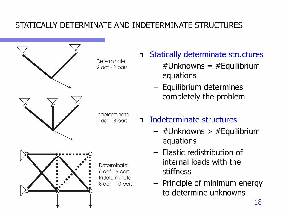
Statically determinate structures
– #Unknowns = #Equilibrium equations
– Equilibrium determines completely the problem
Indeterminate structures
– #Unknowns > #Equilibrium equations
– Elastic redistribution of internal loads with the stiffness
– Principle of minimum energy to determine unknowns
18

PRINCIPLE OF VIRTUAL WORK
▪ Let's define two unrelated states for the body:
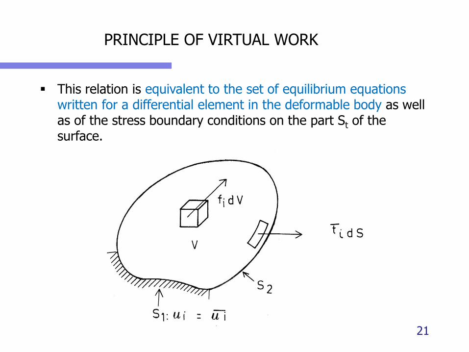
▪ The s-state : This shows external surface forces t, body forces f, and internal stresses s in equilibrium.
▪ The e-state : This shows continuous displacements u* and consistent strains e*.
▪ The superscript * emphasizes that the two states are unrelated.
▪ The principle of virtual work then states: External virtual work is equal to internal virtual work when equilibrated forces and stresses undergo unrelated but consistent displacements and strains.
19

PRINCIPLE OF VIRTUAL WORK
▪ We may specialize the virtual work equation and derive the principle of virtual displacements in variational notations :
▪ Virtual displacements and strains as variations of the real displacements and strains using variational notation such as du = u* and de = e*;
▪ Virtual displacements be zero on the part of the surface that has prescribed displacements, and thus the work done by the reactions is zero. There remains only external surface forces on the part St that do work.
▪ The virtual work equation then becomes the principle of virtual displacements:
20
PRINCIPLE OF VIRTUAL WORK
▪ This relation is equivalent to the set of equilibrium equations written for a differential element in the deformable body as well as of the stress boundary conditions on the part St of the surface.
21

ANALYSIS OF FE DISCRETIZED STRUCTURES
▪ Let's suppose that the body is discrete in nature, for instance truss structure, or it is discretized into finite elements, i.e. continuum structure.
22
▪ The continuous displacement field u(x) in the elements can be approximated using local shape functions N(x) while the unknowns are the nodal displacements, which can be collected in the unknown vector q.
ANALYSIS OF FE DISCRETIZED STRUCTURES
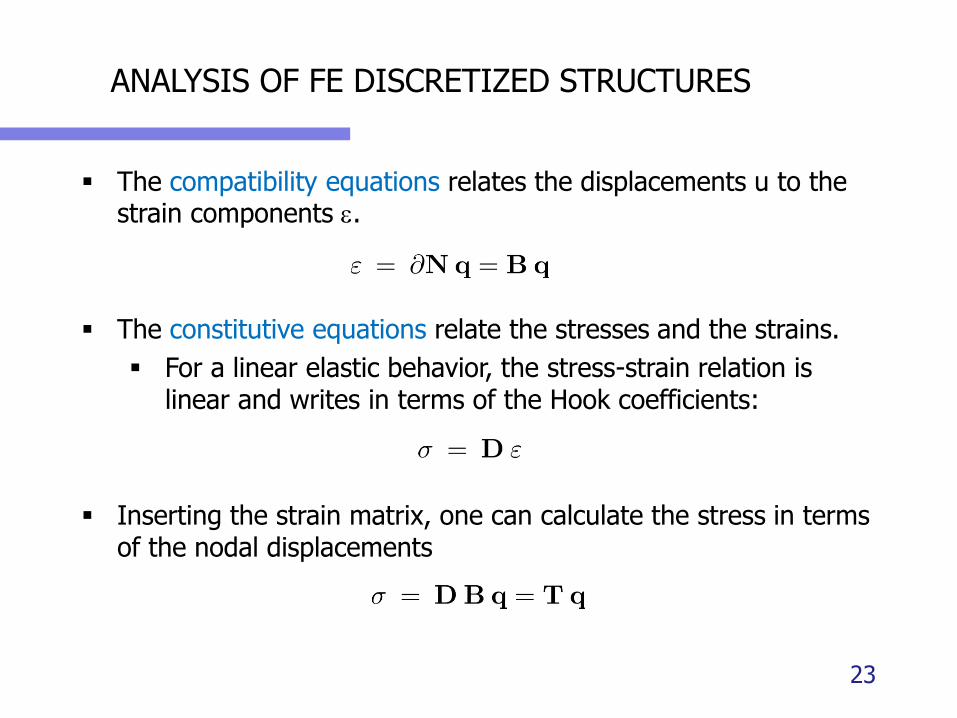
▪ The compatibility equations relates the displacements u to the strain components e.
▪ The constitutive equations relate the stresses and the strains.
▪ For a linear elastic behavior, the stress-strain relation is linear and writes in terms of the Hook coefficients:
▪ Inserting the strain matrix, one can calculate the stress in terms of the nodal displacements
23
ANALYSIS OF FE DISCRETIZED STRUCTURES
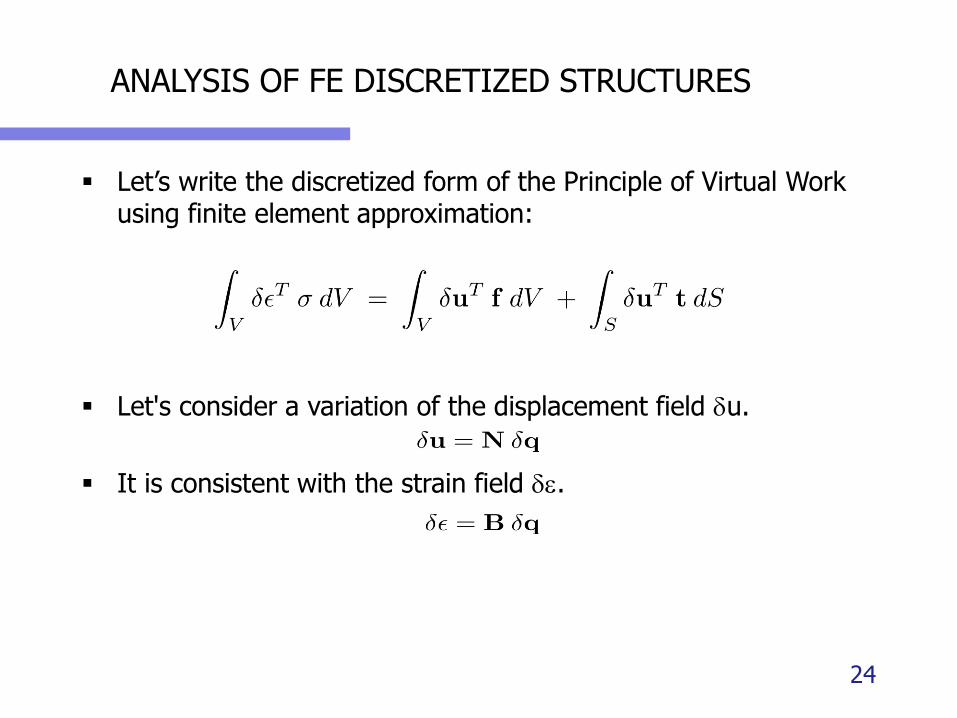
▪ Let’s write the discretized form of the Principle of Virtual Work using finite element approximation:
▪ Let's consider a variation of the displacement field du.
▪ It is consistent with the strain field de.
24
ANALYSIS OF FE DISCRETIZED STRUCTURES
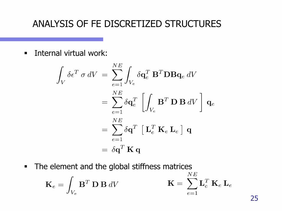
▪ Internal virtual work:
▪ The element and the global stiffness matrices
25

ANALYSIS OF FE DISCRETIZED STRUCTURES
▪ We have now to express the element degrees of freedom in terms of the degrees of freedom of the whole structure. Formally, the element displacement vector can be extracted from la the structural displacement vector by using a localization matrix Le made of a few identity terms placed at the terms to be extracted.
▪ with
26
ANALYSIS OF FE DISCRETIZED STRUCTURES
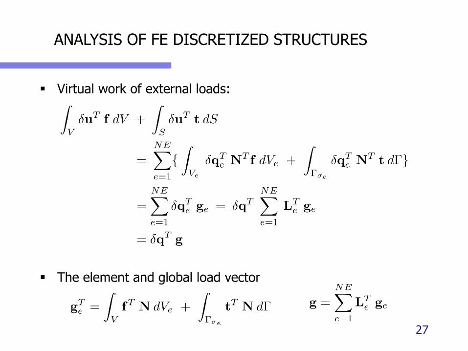
▪ Virtual work of external loads:
▪ The element and global load vector
27

ANALYSIS OF FE DISCRETIZED STRUCTURES
The principle of virtual work discretized with Finite Element approximation writes:
The virtual displacement being arbitrary, the principle of virtual work yields the equilibrium equation
28
INTRODUCTION TO OPTIMALITY CRITERIATWO BAR TRUSS
29
TWO-BAR TRUSS
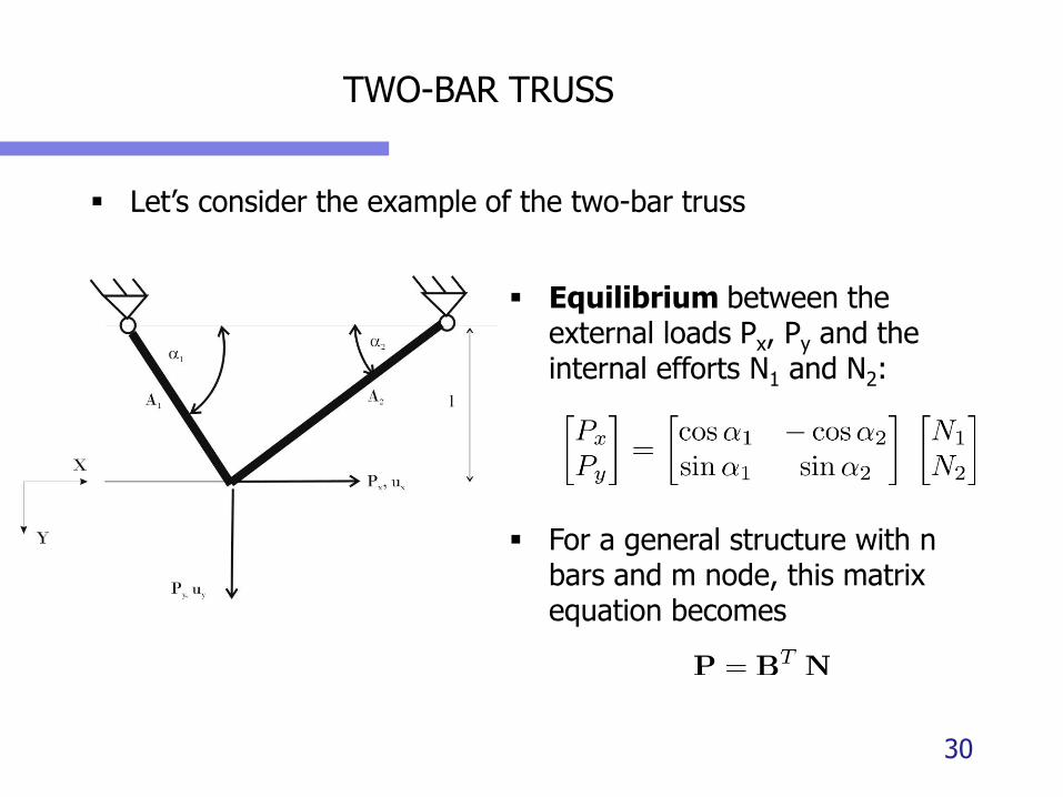
▪ Let’s consider the example of the two-bar truss
30
▪ Equilibrium between the external loads Px, Py and the internal efforts N1 and N2:
▪ For a general structure with n bars and m node, this matrix equation becomes
TWO-BAR TRUSS
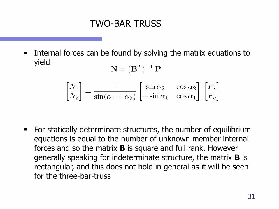
▪ Internal forces can be found by solving the matrix equations to yield
▪ For statically determinate structures, the number of equilibrium equations is equal to the number of unknown member internal forces and so the matrix B is square and full rank. However generally speaking for indeterminate structure, the matrix B is rectangular, and this does not hold in general as it will be seen for the three-bar-truss
31

TWO-BAR TRUSS
▪ Thus for statically determinate structures, the internal bar forces depends only on the applied loads and of the direction cosines of the individual bars.
▪ Stresses
▪ They also depend on the applied load the geometry of the structure and the bar cross sectional areas x*.
32
TWO-BAR TRUSS
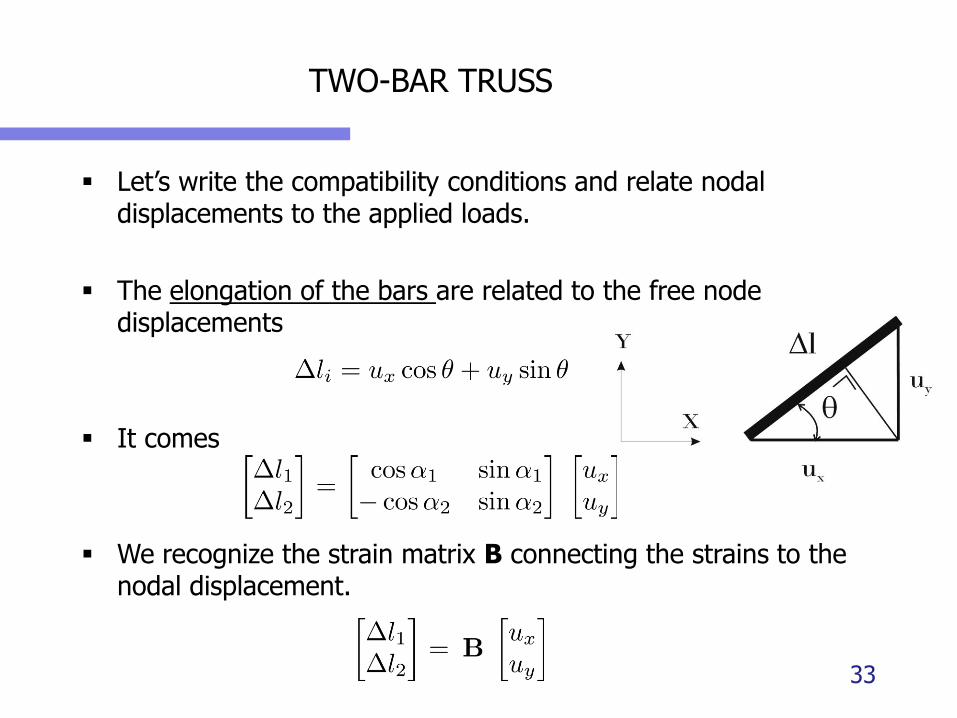
▪ Let’s write the compatibility conditions and relate nodal displacements to the applied loads.
▪ The elongation of the bars are related to the free node displacements
▪ It comes
▪ We recognize the strain matrix B connecting the strains to the nodal displacement.
33
TWO-BAR TRUSS
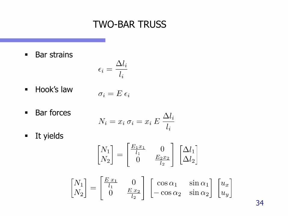
▪ Bar strains
▪ Hook’s law
▪ Bar forces
▪ It yields
34
TWO-BAR TRUSS
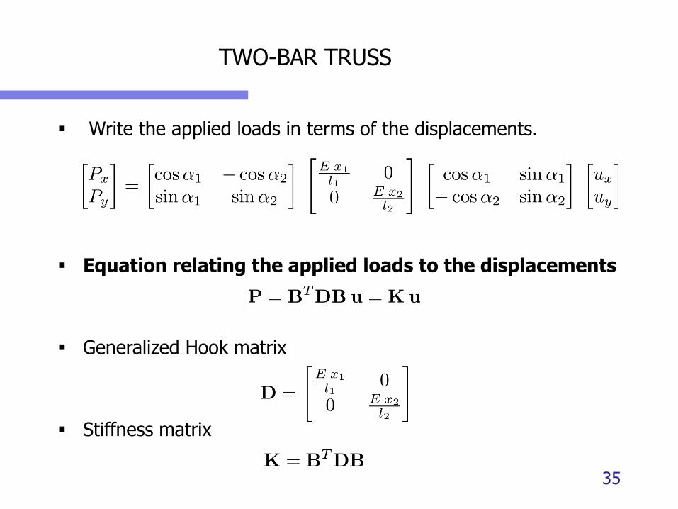
▪ Write the applied loads in terms of the displacements.
▪ Equation relating the applied loads to the displacements
▪ Generalized Hook matrix
▪ Stiffness matrix
35
TWO-BAR TRUSS
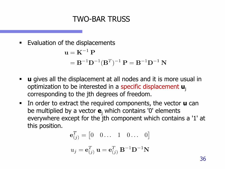
▪ Evaluation of the displacements
▪ u gives all the displacement at all nodes and it is more usual in optimization to be interested in a specific displacement uj
corresponding to the jth degrees of freedom.
▪ In order to extract the required components, the vector u can be multiplied by a vector ej which contains '0' elements everywhere except for the jth component which contains a '1' at this position.
36
TWO-BAR TRUSS
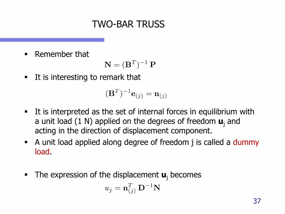
▪ Remember that
▪ It is interesting to remark that
▪ It is interpreted as the set of internal forces in equilibrium with a unit load (1 N) applied on the degrees of freedom uj and acting in the direction of displacement component.
▪ A unit load applied along degree of freedom j is called a dummy load.
▪ The expression of the displacement uj becomes
37
TWO-BAR TRUSS
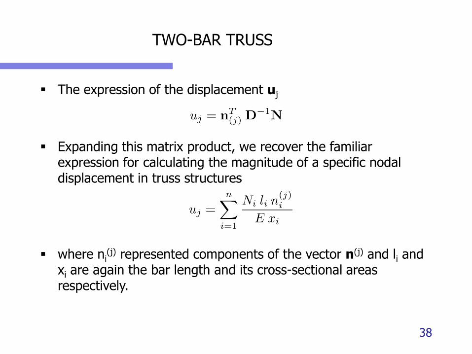
▪ The expression of the displacement uj
▪ Expanding this matrix product, we recover the familiar expression for calculating the magnitude of a specific nodal displacement in truss structures
▪ where ni(j) represented components of the vector n(j) and li and
xi are again the bar length and its cross-sectional areasrespectively.
38
TWO-BAR TRUSS
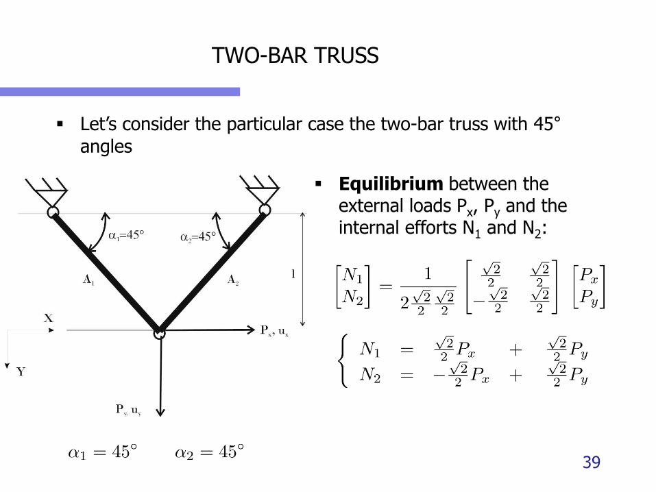
▪ Let’s consider the particular case the two-bar truss with 45°angles
39
▪ Equilibrium between the external loads Px, Py and the internal efforts N1 and N2:
TWO –BAR TRUSS
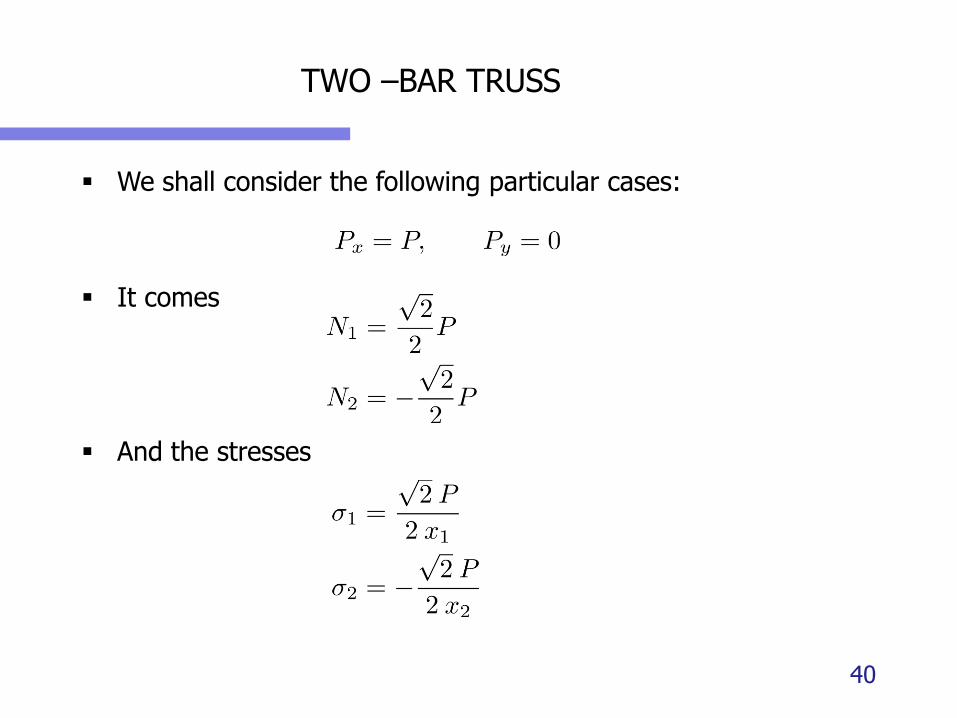
▪ We shall consider the following particular cases:
▪ It comes
▪ And the stresses
40
TWO-BAR TRUSS
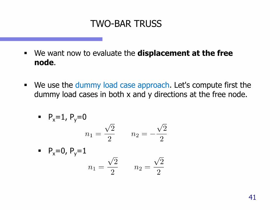
▪ We want now to evaluate the displacement at the free node.
▪ We use the dummy load case approach. Let's compute first the dummy load cases in both x and y directions at the free node.
▪ Px=1, Py=0
▪ Px=0, Py=1
41
TWO-BAR TRUSS
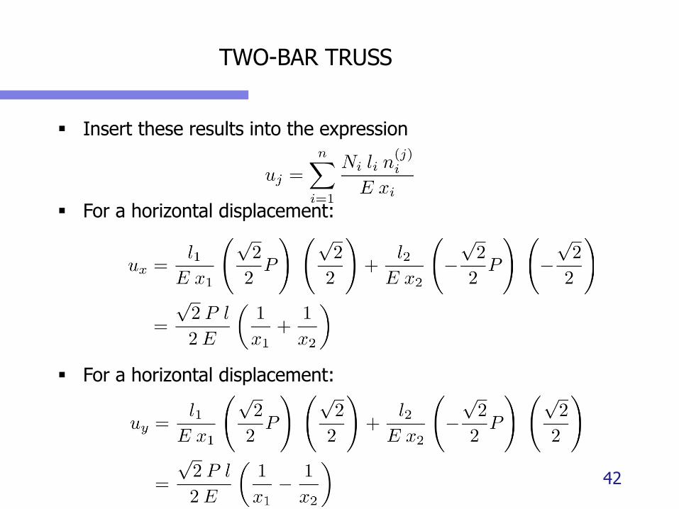
▪ Insert these results into the expression
▪ For a horizontal displacement:
▪ For a horizontal displacement:
42
TWO-BAR TRUSS
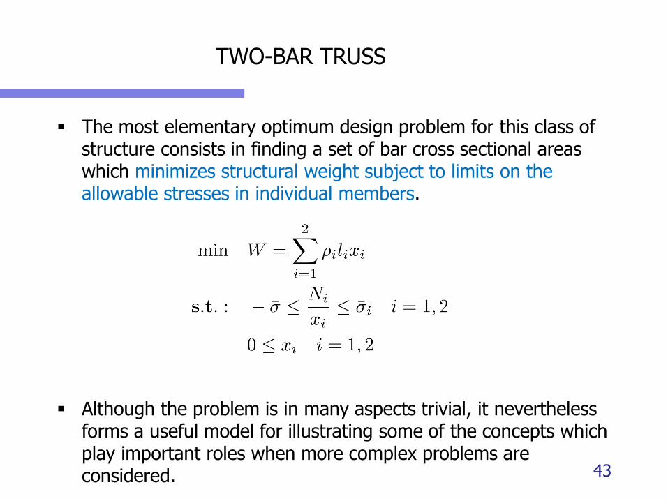
▪ The most elementary optimum design problem for this class of structure consists in finding a set of bar cross sectional areas which minimizes structural weight subject to limits on the allowable stresses in individual members.
▪ Although the problem is in many aspects trivial, it nevertheless forms a useful model for illustrating some of the concepts which play important roles when more complex problems are considered. 43
TWO-BAR TRUSS
44
TWO-BAR TRUSS
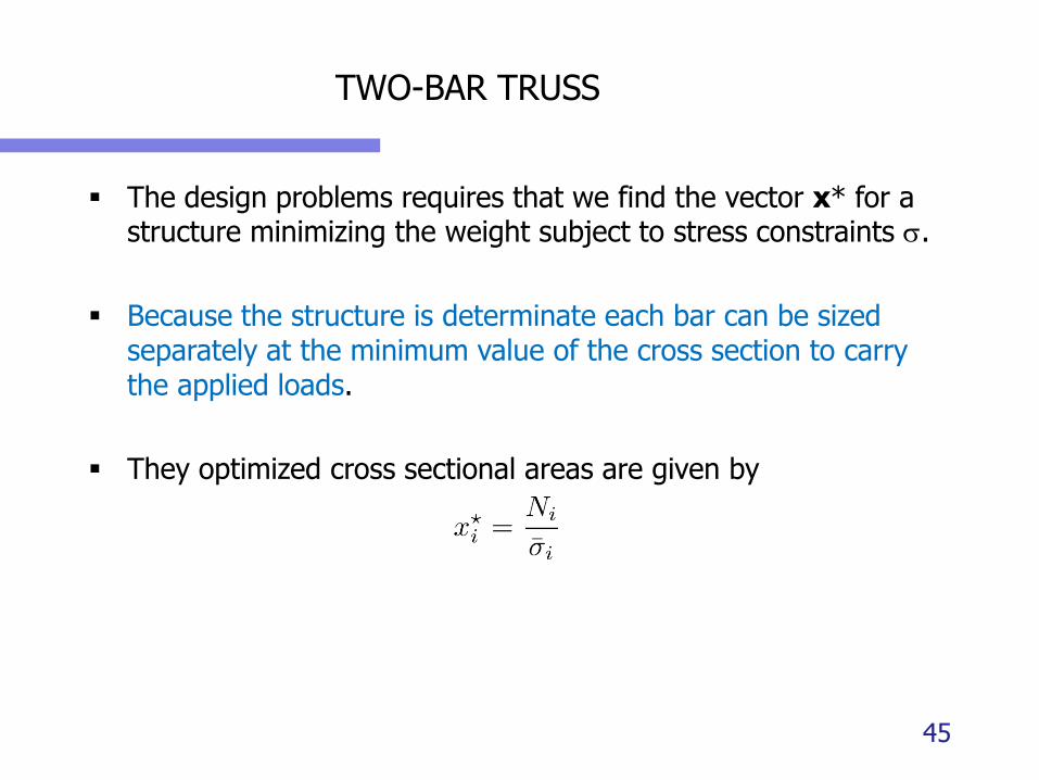
▪ The design problems requires that we find the vector x* for a structure minimizing the weight subject to stress constraints s.
▪ Because the structure is determinate each bar can be sized separately at the minimum value of the cross section to carry the applied loads.
▪ They optimized cross sectional areas are given by
45
TWO-BAR TRUSS
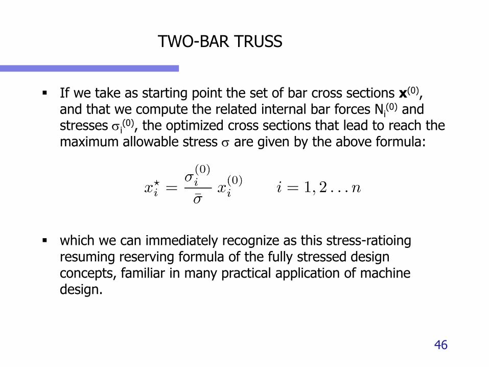
▪ If we take as starting point the set of bar cross sections x(0), and that we compute the related internal bar forces Ni
(0) and stresses si
(0), the optimized cross sections that lead to reach the maximum allowable stress s are given by the above formula:
▪ which we can immediately recognize as this stress-ratioing resuming reserving formula of the fully stressed design concepts, familiar in many practical application of machine design.
46
TWO BAR TRUSS
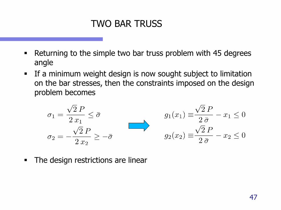
▪ Returning to the simple two bar truss problem with 45 degrees angle
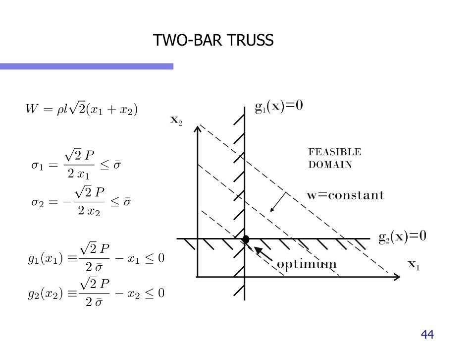
▪ If a minimum weight design is now sought subject to limitation on the bar stresses, then the constraints imposed on the design problem becomes
▪ The design restrictions are linear
47

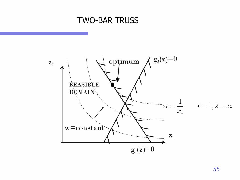
TWO-BAR TRUSS
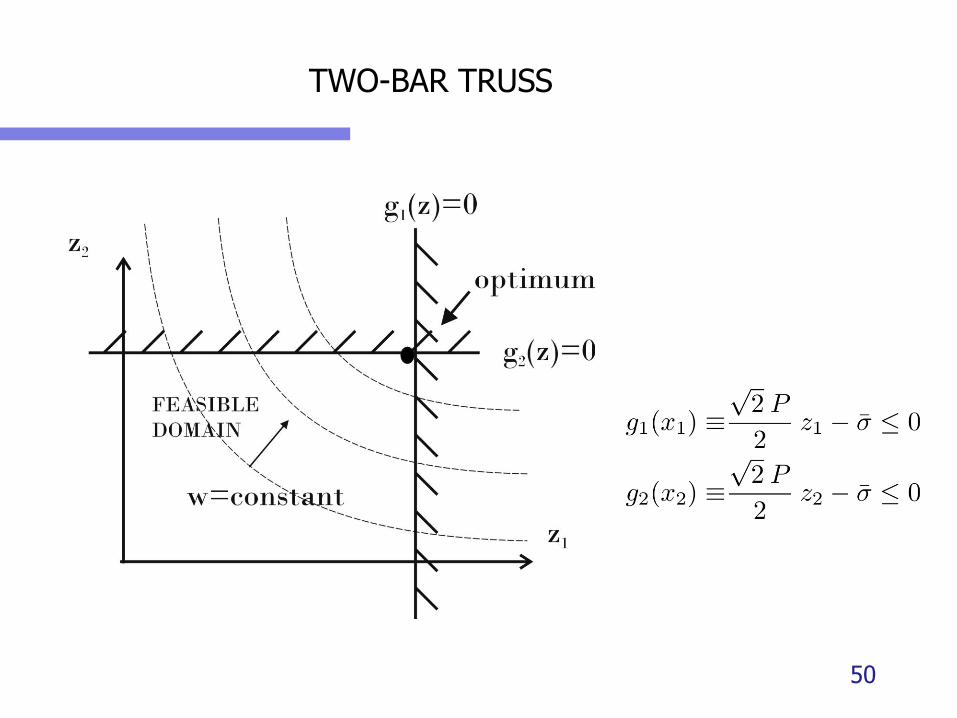
▪ The problem is linear, and the constraints are parallel to the axis defined by the design variables x1, and x2.
▪ It is clearly seen that each of these variable is associated with one and only one constraint and then the optimum design occurs at a vertex in design space.
▪ The optimum can therefore be fought by seeking to simultaneously satisfy the design constraints rather than seeking to actually minimize the objective function.
48
TWO-BAR TRUSS
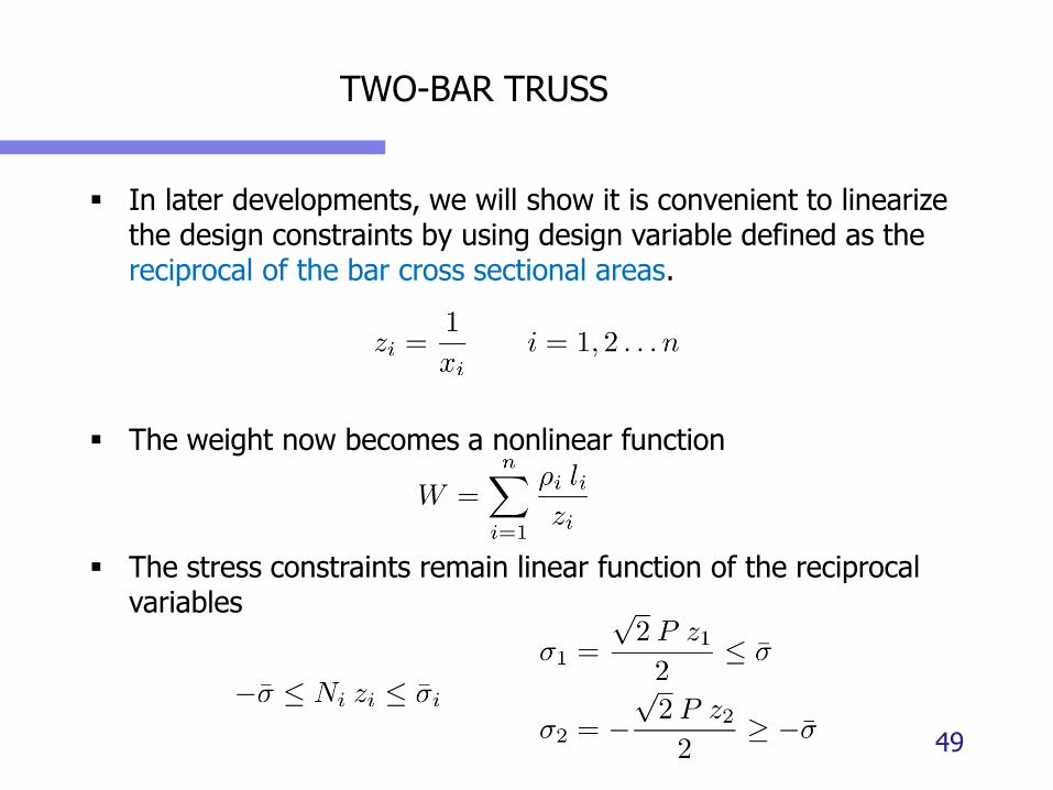
▪ In later developments, we will show it is convenient to linearize the design constraints by using design variable defined as the reciprocal of the bar cross sectional areas.
▪ The weight now becomes a nonlinear function
▪ The stress constraints remain linear function of the reciprocal variables
49
TWO-BAR TRUSS
50
TWO-BAR TRUSS
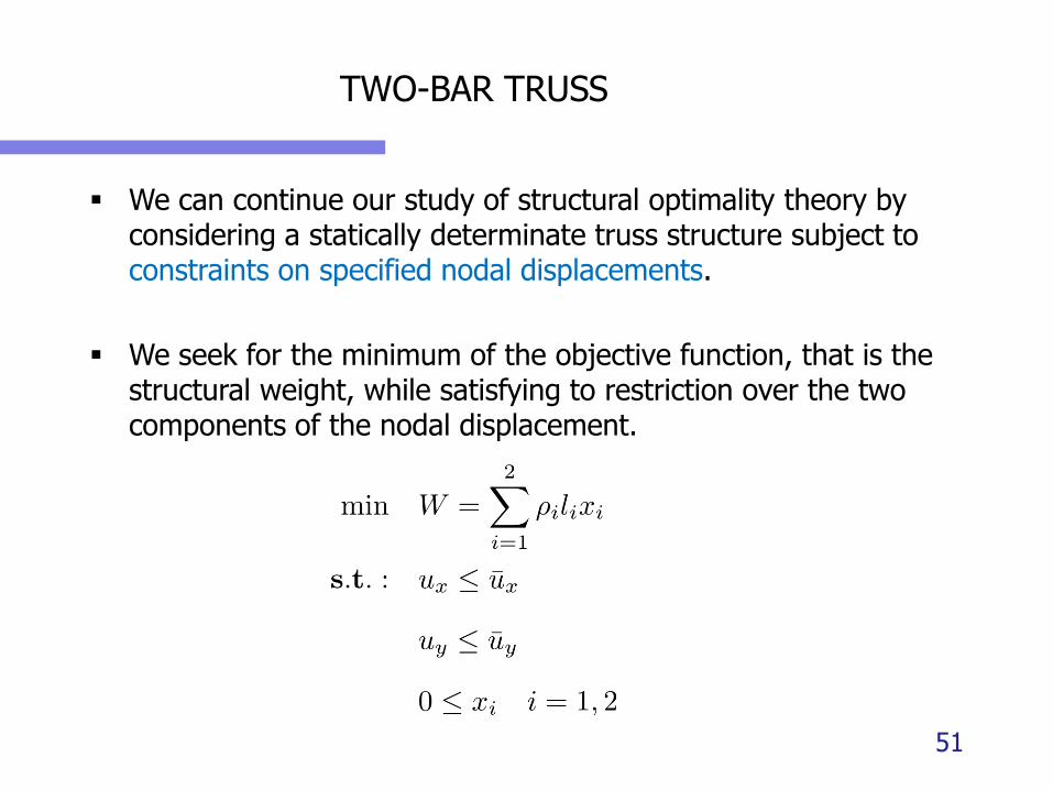
▪ We can continue our study of structural optimality theory by considering a statically determinate truss structure subject to constraints on specified nodal displacements.
▪ We seek for the minimum of the objective function, that is the structural weight, while satisfying to restriction over the two components of the nodal displacement.
51
TWO-BAR TRUSS
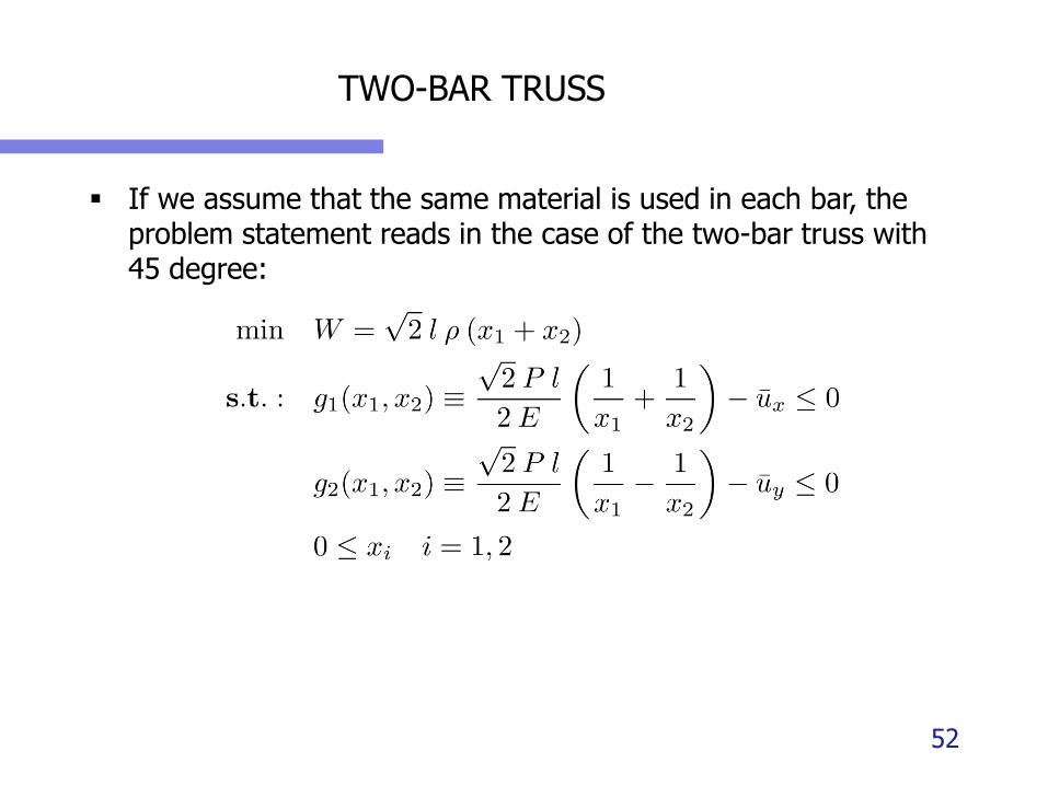
▪ If we assume that the same material is used in each bar, the problem statement reads in the case of the two-bar truss with 45 degree:
52

TWO-BAR TRUSS
▪ If the cross-sectional areas are taken as design variables, the problem may not be convex as it is usually illustrated by returning to the two-bar example.
53
TWO-BAR TRUSS
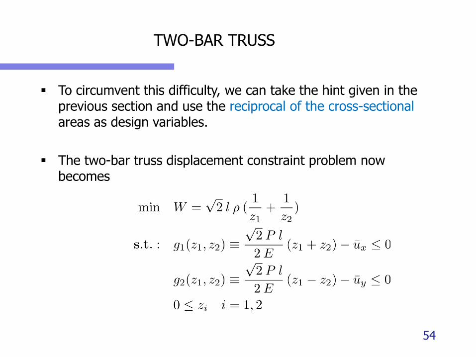
▪ To circumvent this difficulty, we can take the hint given in the previous section and use the reciprocal of the cross-sectional areas as design variables.
▪ The two-bar truss displacement constraint problem now becomes
54
TWO-BAR TRUSS
55

OPTIMALITY CRITERIA
Principle of Virtual Work and Finite Element notations
Optimality criteria for fully stressed design
Berke’s approximation of displacement
Optimality criteria for a single displacement constraint
Optimality criteria for several displacement and stress constraints
5656

OPTIMALITY CRITERIA
▪ General approach adopted by Optimality Criteria applied to the mass minimization problems
▪ Write a priori the conditions that must be satisfied by theoptimal design.
▪ KKT conditions of the optimum design problem
▪ Based on isostatic problems
▪ Deduce a recursive relation to be iteratively applied to obtain the optimal design
▪ “Primal design variables” (sizing variables) are given in term of the “dual variables” (Lagrange multipliers)
▪ Update of “dual variables” (Lagrange multipliers) to satisfy the active constraints (and KKT conditions)
57
OPTIMALITY CRITERIA
▪ 1/ Optimality conditions are derived for isostatic (determinate) structures.
▪ ➔ exact solution in that particular case
▪ ➔ convergence in 1 iteration
▪ 2/ Extension to the general case of hyperstatic (indeterminate) structures
▪ ➔ approximate solution
▪ ➔ iterative scheme
58
OPTIMALITY CRITERIA
▪ Identified difficulties
▪ Select a priori the set of active constraints that will be used in the optimality conditions
▪ Convergence to design points which are not necessarily KKTpoint for the general case
59
OPTIMALITY CRITERIA
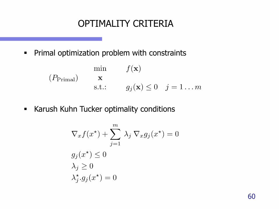
▪ Primal optimization problem with constraints
▪ Karush Kuhn Tucker optimality conditions
60

FULLY STRESSED DESIGN
61

FULLY STRESSED DESIGN
▪ The first considered optimality criteria is the most famous one: Fully Stressed Design
▪ It is founded on the intuitive hypothesis, but non analytically justified, that all components in the optimized structure reach simultaneously their maximum allowable stress, generally calculated based on a linear elastic analysis.
▪ It is simple, easy to implement, fast convergent
▪ Often used by engineers in practice for structures subject to stress restrictions only.
62
FULLY STRESSED DESIGN
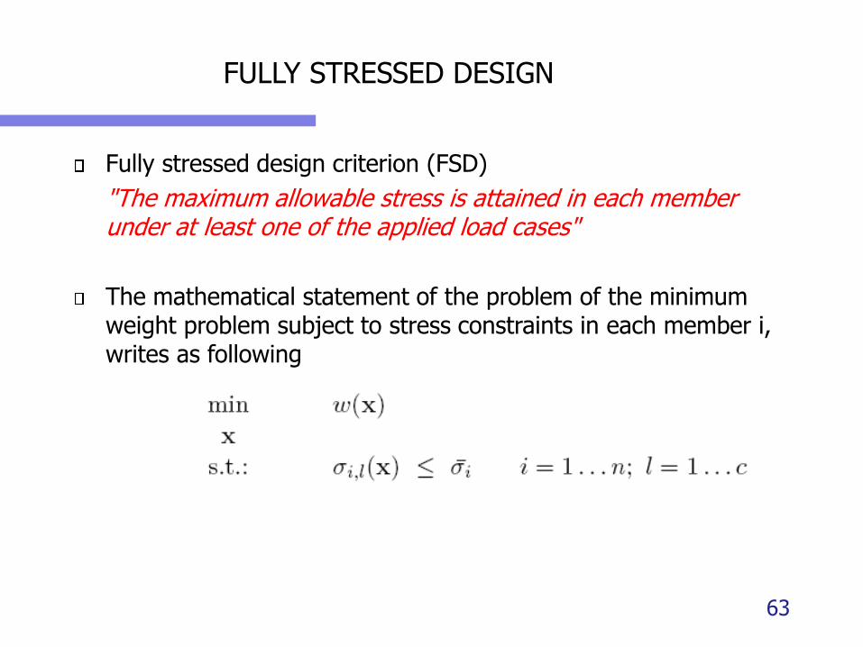
Fully stressed design criterion (FSD)
"The maximum allowable stress is attained in each member under at least one of the applied load cases"
The mathematical statement of the problem of the minimum weight problem subject to stress constraints in each member i, writes as following
63
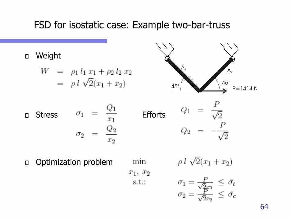
FSD for isostatic case: Example two-bar-truss
Weight
Stress Efforts
Optimization problem
64

FSD for isostatic case: Example two-bar-truss
Optimum (analytical solution)
Redesign formula
If one performs a first analysis (which is not optimal) with the set of design variables x(0):
65

FSD for isostatic case: Example two-bar-truss
FSD is exact in this case, because the two-bar-truss is a determinate structure.
It is true for all statically determinate structures, because the internal efforts are constant and do not depend on the stiffness distribution.
If one adds one bar (three bar truss), the truss is indeterminate, and the efforts depends on all the design variables. ➔ FSD
becomes an approximation
66
FULLY STRESSED DESIGN
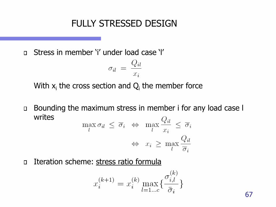
Stress in member ‘i’ under load case ‘l’
With xi the cross section and Qi the member force
Bounding the maximum stress in member i for any load case l writes
Iteration scheme: stress ratio formula
67

FULLY STRESSED DESIGN
Stress ratio formula
The formula is rigorous for one single load case, one material.
For statically indeterminate structures, the FSD is approximate.
FSD can be extended to other elements than truss structures, for instance by considering the von Mises stress (e.g. in plane stress plate) in the stress ratio formula
68
FULLY STRESSED DESIGN
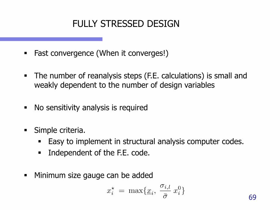
▪ Fast convergence (When it converges!)
▪ The number of reanalysis steps (F.E. calculations) is small and weakly dependent to the number of design variables
▪ No sensitivity analysis is required
▪ Simple criteria.
▪ Easy to implement in structural analysis computer codes.
▪ Independent of the F.E. code.
▪ Minimum size gauge can be added
69
FULLY STRESSED DESIGN
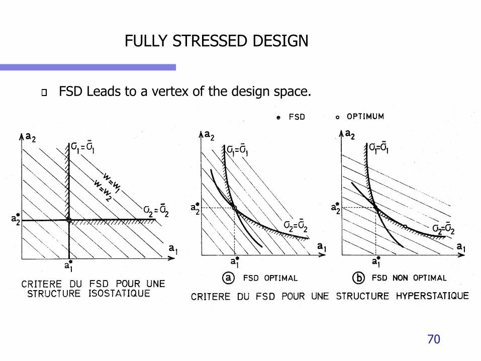
FSD Leads to a vertex of the design space.
70

FSD for general case (hyperstatic)
▪ FSD replaces the stress restrictions by hyperplanes parallel to the axes
▪ The objective function disappears from the formulation
▪ Provided that all coefficient in the objective function are positive
▪ Solution is always located in a vertex of the design space
▪ Not always the case when strongly hyperstatic problems with redistribution of the internal loads
▪ In these cases, it can lead to non optimal solutions and oscillatory convergence processes.
71
72
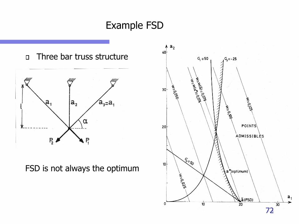
Example FSD
Three bar truss structure
FSD is not always the optimum
72
73
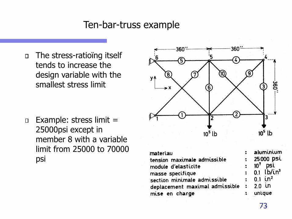
Ten-bar-truss example
The stress-ratioïng itself tends to increase the design variable with the smallest stress limit
Example: stress limit = 25000psi except in member 8 with a variable limit from 25000 to 70000 psi
73

Ten-bar-truss example
74
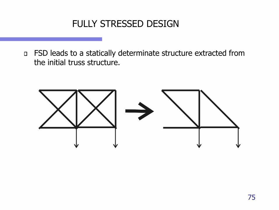
FULLY STRESSED DESIGN
FSD leads to a statically determinate structure extracted from the initial truss structure.
75
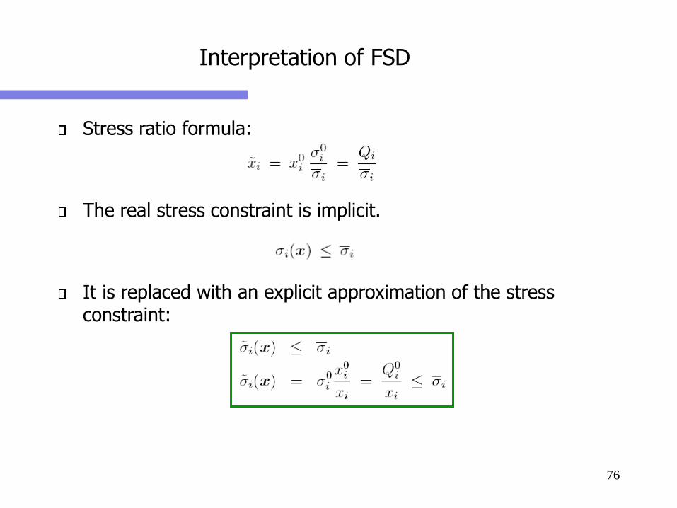
Interpretation of FSD
Stress ratio formula:
The real stress constraint is implicit.
It is replaced with an explicit approximation of the stress constraint:
76

Interpretation of FSD
The value of the approximation is exact in x0
It is also exact along the scaling line
The derivatives are not respected
FSD ➔ Zero order approximation
in x0 (and also along the scaling line)
77
Berke’s approximation
78

ANALYSIS OF FE DISCRETIZED STRUCTURES
▪ Let's consider a system with known actual deformations e, which are supposedly consistent, giving rise to displacements u throughout the system.
▪ For example, a point P has moved to P', and one wants to compute the displacement uP of P in a considered direction n.
▪ For this particular purpose, we choose the following virtual unit force system:
▪ The unit force F(1) is located at P and acts in the direction of n so that the external virtual work done by F(1) is, noting that the displacement in P along direction n.
▪ The internal virtual work done by the virtual stresses is
79
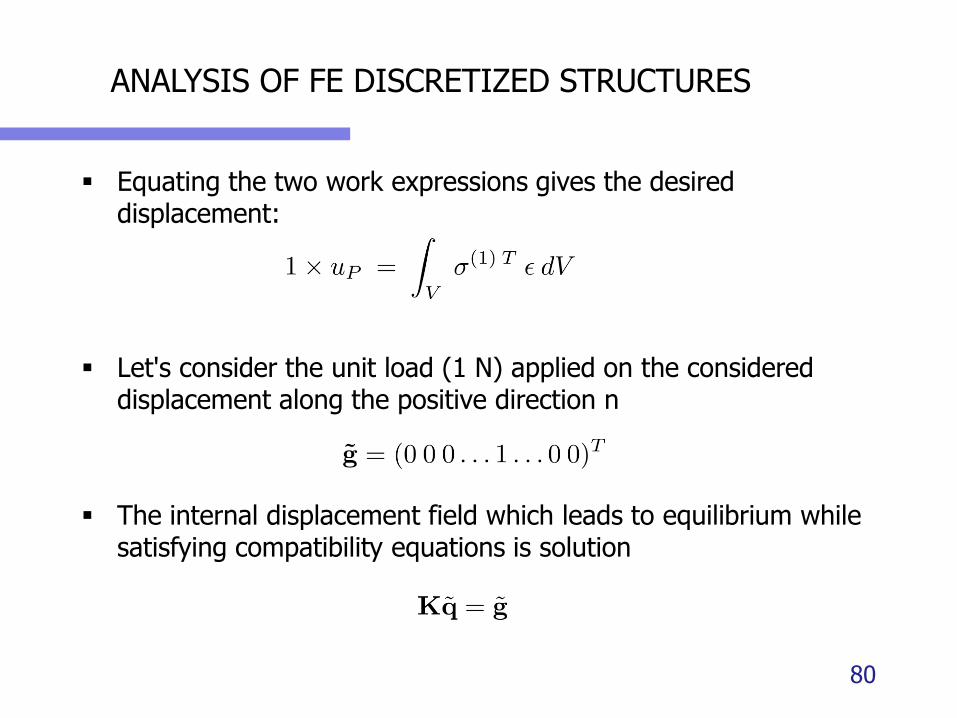
ANALYSIS OF FE DISCRETIZED STRUCTURES
▪ Equating the two work expressions gives the desired displacement:
▪ Let's consider the unit load (1 N) applied on the considered displacement along the positive direction n
▪ The internal displacement field which leads to equilibrium while satisfying compatibility equations is solution
80
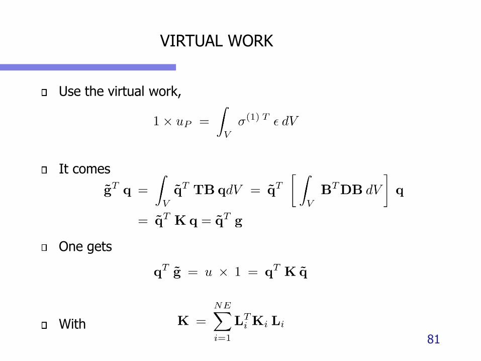
VIRTUAL WORK
Use the virtual work,
It comes
One gets
With 81

VIRTUAL WORK
For many design variables, the stiffness matrix takes the interesting form:
For instance:
– Truss structures xi =Ai
– Plate structures xi =ti– Beam structures xi =hi³
– Shell structures xi =ti³
82
VIRTUAL WORK
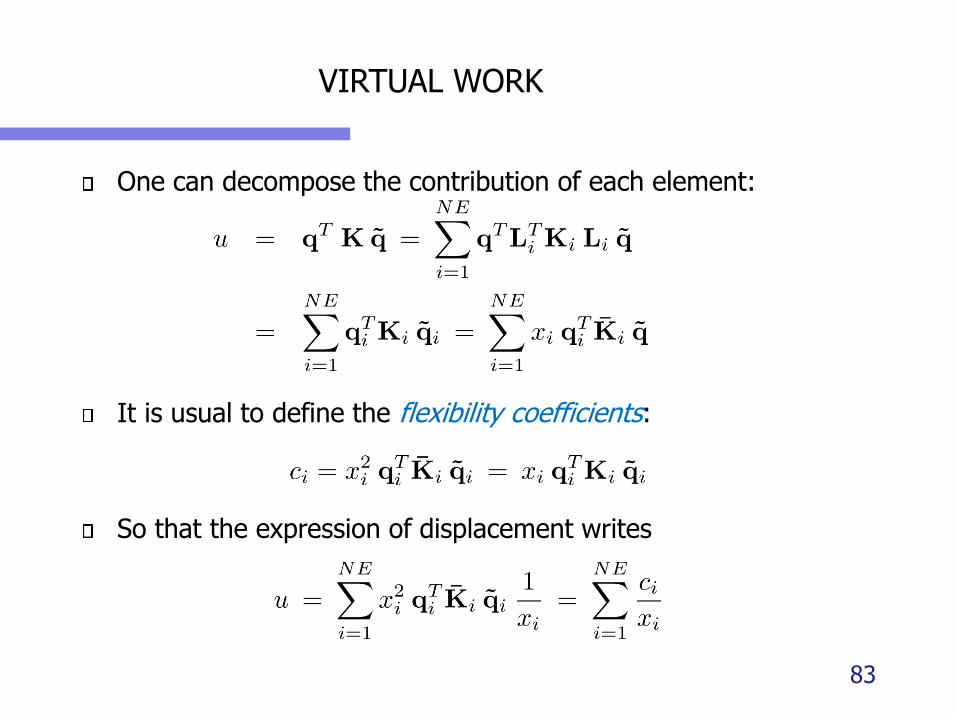
One can decompose the contribution of each element:
It is usual to define the flexibility coefficients:
So that the expression of displacement writes
83
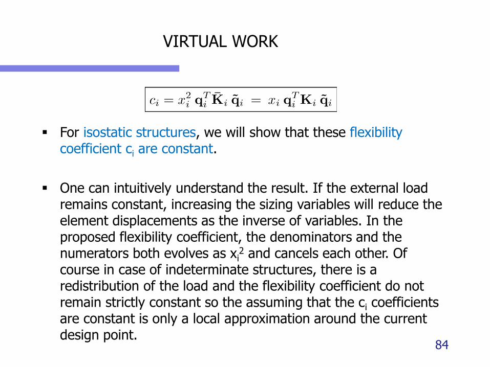
VIRTUAL WORK
▪ For isostatic structures, we will show that these flexibility coefficient ci are constant.
▪ One can intuitively understand the result. If the external load remains constant, increasing the sizing variables will reduce the element displacements as the inverse of variables. In the proposed flexibility coefficient, the denominators and the numerators both evolves as xi
2 and cancels each other. Of course in case of indeterminate structures, there is a redistribution of the load and the flexibility coefficient do not remain strictly constant so the assuming that the ci coefficients are constant is only a local approximation around the current design point.
84
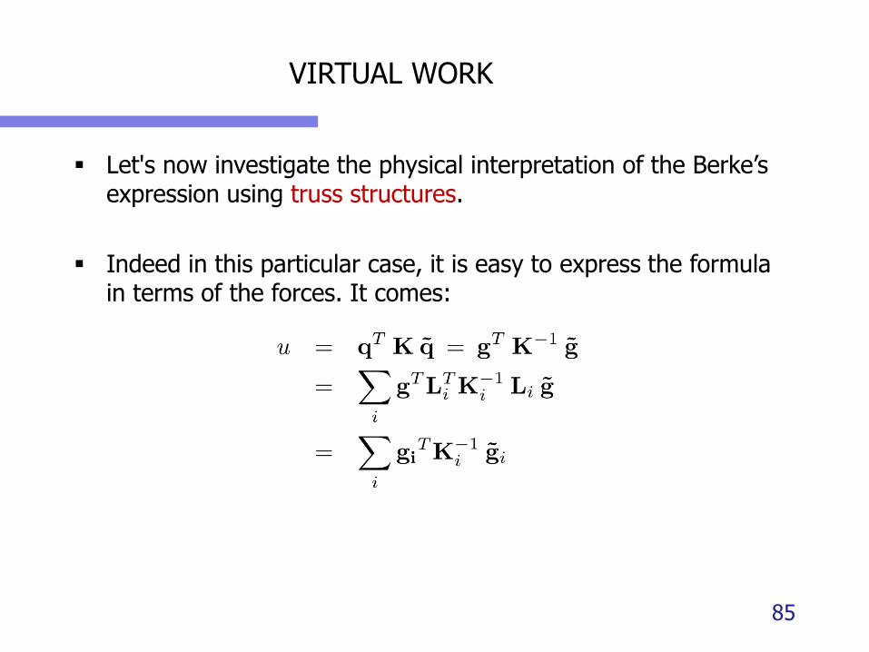
VIRTUAL WORK
▪ Let's now investigate the physical interpretation of the Berke’s expression using truss structures.
▪ Indeed in this particular case, it is easy to express the formula in terms of the forces. It comes:
85
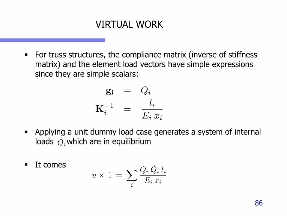
VIRTUAL WORK
▪ For truss structures, the compliance matrix (inverse of stiffness matrix) and the element load vectors have simple expressions since they are simple scalars:
▪ Applying a unit dummy load case generates a system of internal loads which are in equilibrium
▪ It comes
86
VIRTUAL WORK
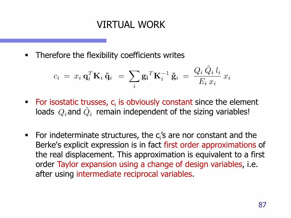
▪ Therefore the flexibility coefficients writes
▪ For isostatic trusses, ci is obviously constant since the element loads and remain independent of the sizing variables!
▪ For indeterminate structures, the ci’s are nor constant and the Berke's explicit expression is in fact first order approximations of the real displacement. This approximation is equivalent to a first order Taylor expansion using a change of design variables, i.e. after using intermediate reciprocal variables.
87
VIRTUAL WORK
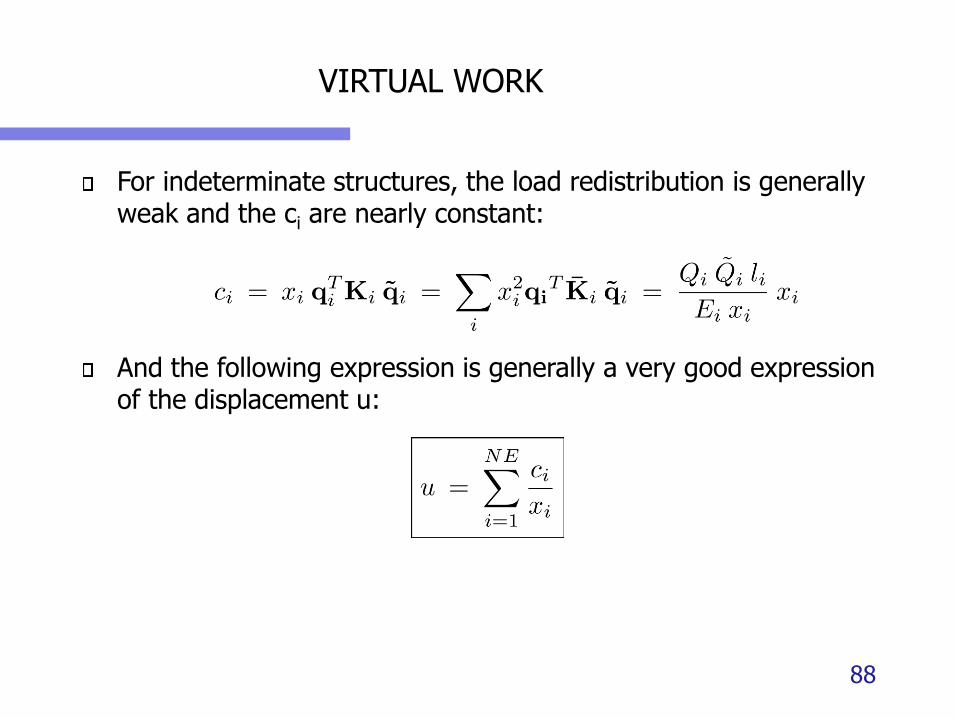
For indeterminate structures, the load redistribution is generally weak and the ci are nearly constant:
And the following expression is generally a very good expression of the displacement u:
88
Berke’s expression is a first order approximation
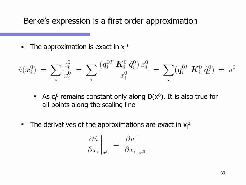
▪ The approximation is exact in xi0
▪ As ci0 remains constant only along D(x0). It is also true for
all points along the scaling line
▪ The derivatives of the approximations are exact in xi0
89
Berke’s expression is a first order approximation
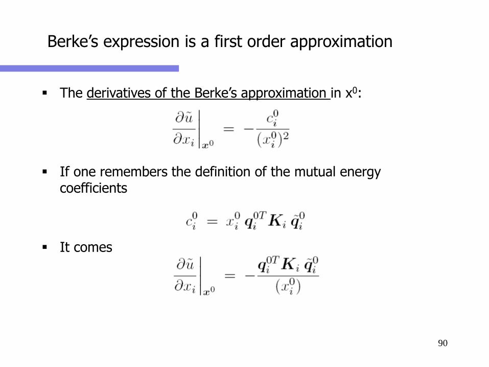
▪ The derivatives of the Berke’s approximation in x0:
▪ If one remembers the definition of the mutual energy coefficients
▪ It comes
90

Berke’s expression is a first order approximation
▪ The true derivative of the displacement function with respect to xi can be calculated as follows
▪ It comes
91
Berke’s expression is a first order approximation
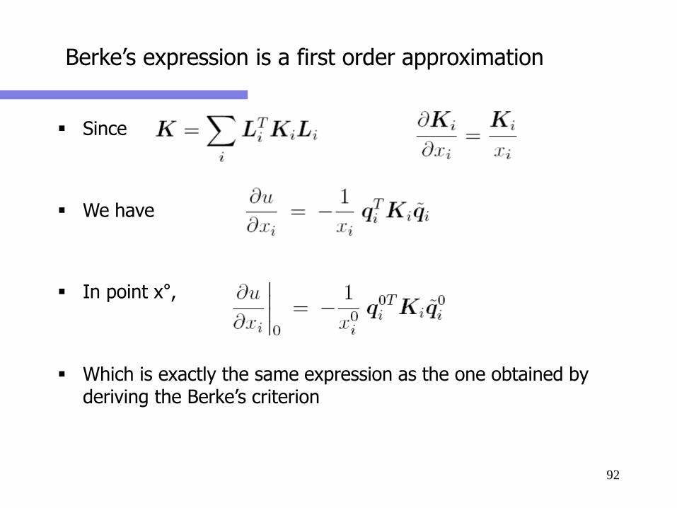
▪ Since
▪ We have
▪ In point x°,
▪ Which is exactly the same expression as the one obtained by deriving the Berke’s criterion
92
Berke’s expression is a first order approximation
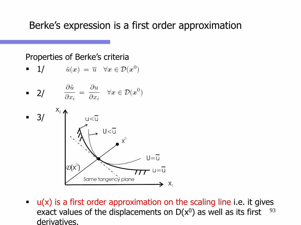
Properties of Berke’s criteria
▪ 1/
▪ 2/
▪ 3/
▪ u(x) is a first order approximation on the scaling line i.e. it gives exact values of the displacements on D(x0) as well as its first derivatives.
93
OPTIMALITY CRITERIA FOR A SINGLE DISPLACEMENT
CONSTRAINT
94

Single displacement constraint
Let's come back to the minimum weight design problem. One considers the problem with a single displacement constraint:
Virtual loading case (unit load) in the direction of the displacement u
Decomposition in the contributions of each element:
– ci constant for a statically determinate structure.95

Single displacement constraint
Explicit problem:
Let’s introduce a Lagrange multiplier and shape the Lagrange function
Stationary conditions
96

Single displacement constraint
If ci is positive: OK!
If ci is less or equal to zero: → passive variables
To identify the Lagrange variable , one substitutes the xi by its value into the constraint that displacement an equality constraint:
Let’s define
97

Single displacement constraint
Let’s identify the Lagrange multiplier :
So it comes
98

Single displacement constraint
Physical meaning of the optimality criteria
– Strain energy
– Virtual strain energy
Let's define the virtual strain energy of bar ‘i’
The energy density of bar ‘i’ is the energy of bar ‘i’ divided by the weight of this bar
99
Single displacement constraint
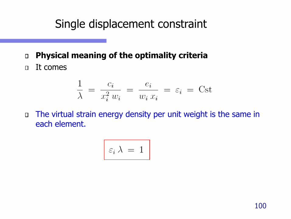
Physical meaning of the optimality criteria
It comes
The virtual strain energy density per unit weight is the same in each element.
100
Single displacement constraint
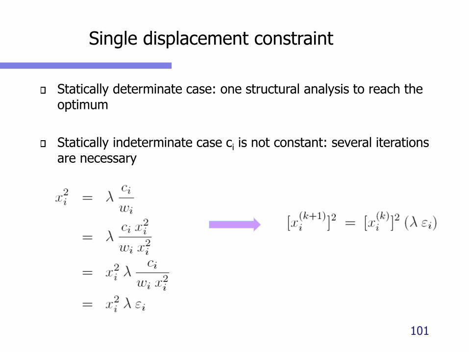
Statically determinate case: one structural analysis to reach the optimum
Statically indeterminate case ci is not constant: several iterations are necessary
101
Single displacement constraint
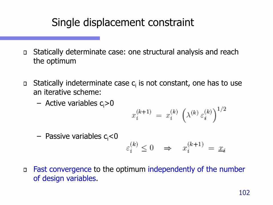
Statically determinate case: one structural analysis and reach the optimum
Statically indeterminate case ci is not constant, one has to use an iterative scheme:
– Active variables ci>0
– Passive variables ci<0
Fast convergence to the optimum independently of the number of design variables.
102

Two bar truss example
Minimum weight design subject to a horizontal displacement constraint
The virtual work theorem
Weight of the truss
103
Two bar truss example
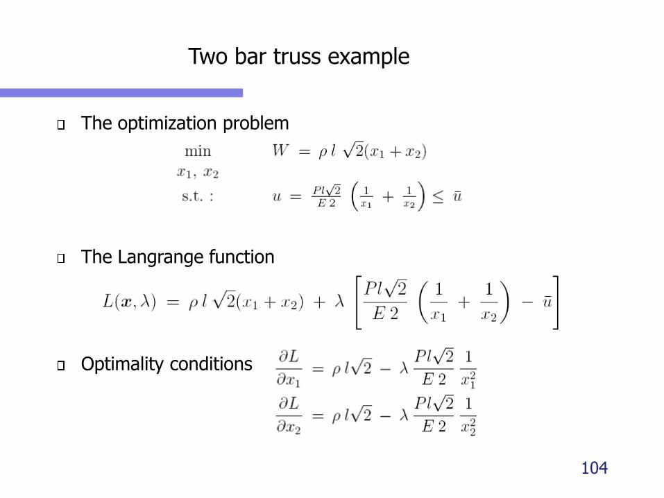
The optimization problem
The Langrange function
Optimality conditions
104
Two bar truss example
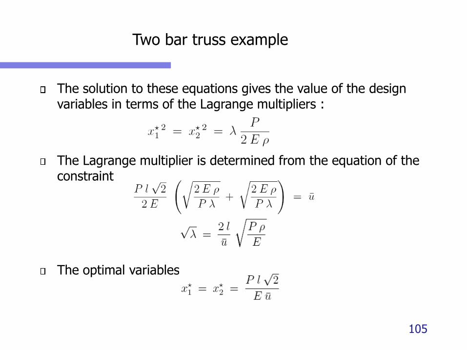
The solution to these equations gives the value of the design variables in terms of the Lagrange multipliers :
The Lagrange multiplier is determined from the equation of the constraint
The optimal variables
105
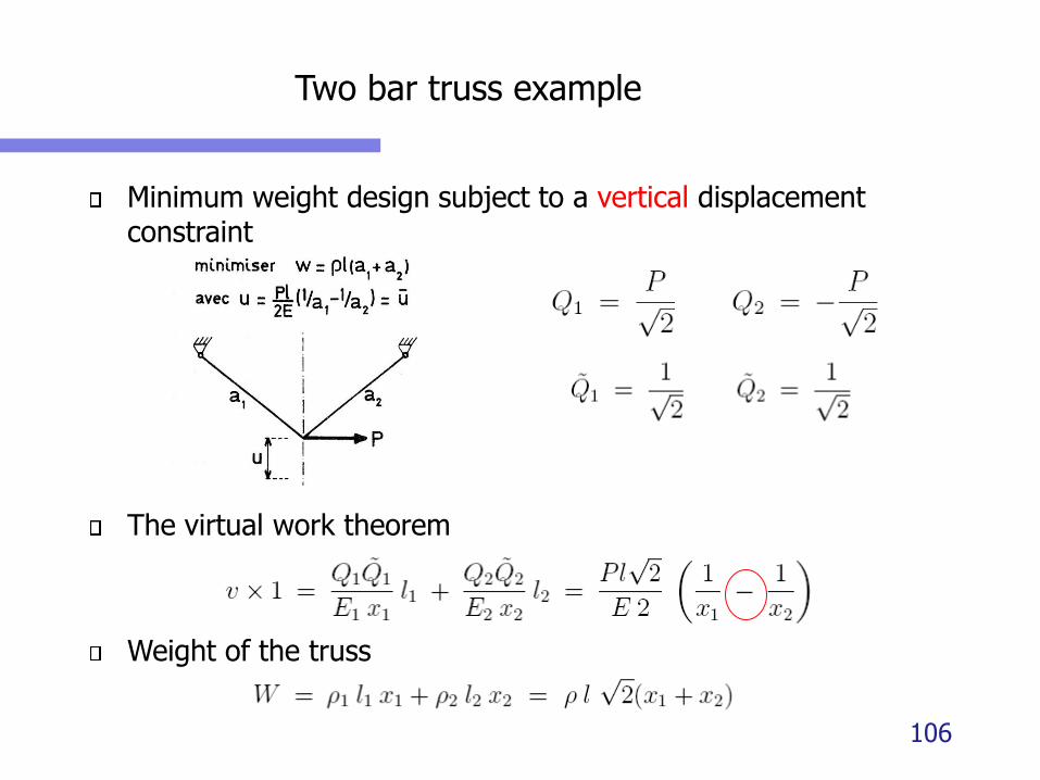
Two bar truss example
Minimum weight design subject to a vertical displacement constraint
The virtual work theorem
Weight of the truss
106
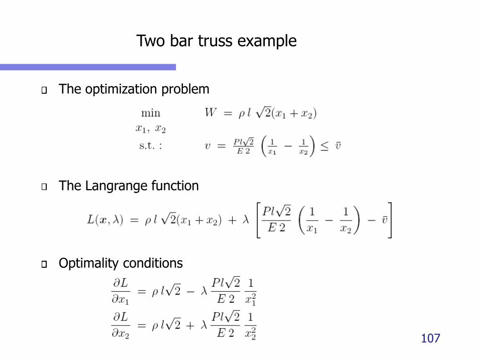
Two bar truss example
The optimization problem
The Langrange function
Optimality conditions
107

Two bar truss example
This means that the variables x1 and x2 can be as small as we want while satisfying the constraint on the displacement constraint on v. It is the minimum gauge on x2 which determines the optimum
108
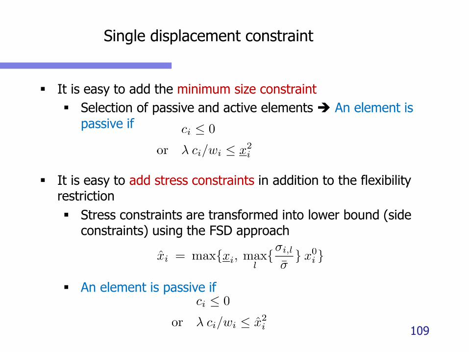
Single displacement constraint
▪ It is easy to add the minimum size constraint
▪ Selection of passive and active elements ➔ An element is
passive if
▪ It is easy to add stress constraints in addition to the flexibility restriction
▪ Stress constraints are transformed into lower bound (side constraints) using the FSD approach
▪ An element is passive if
109
Single displacement constraint
▪ For isostatic structures,
▪ Solution exact in one structural (Finite Element) analysis
▪ Redesign criteria must may be applied iteratively when the active / passive design variable set has to be selected when restrictions are imposed on the minimum size or by stress constraints (FSD)
▪ For hyperstatic structures
▪ Ci’s are not constant because of the load redistribution
▪ Redesign criteria must be applied iteratively.
▪ Fast convergence.
▪ Generally non convergence problems are related to the stress constraints which are not accounting (approximated) accurately
110
OPTIMALITY CRITERIA :MULTIPLE DISPLACEMENT AND STRESS CONSTRAINTS
111
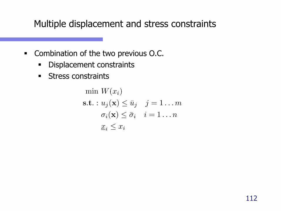
Multiple displacement and stress constraints
▪ Combination of the two previous O.C.
▪ Displacement constraints
▪ Stress constraints
112
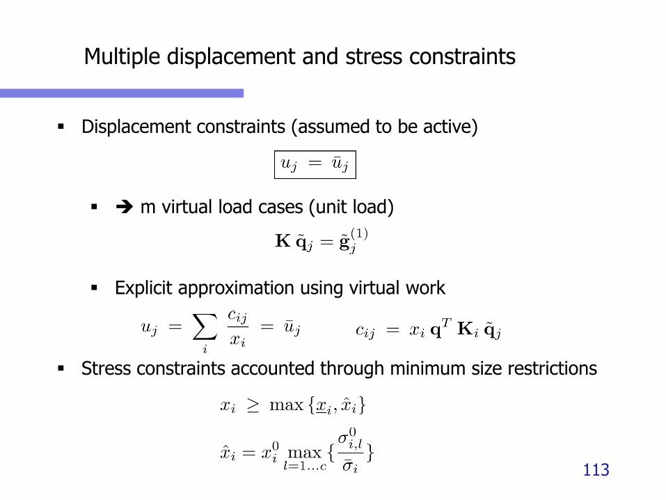
Multiple displacement and stress constraints
▪ Displacement constraints (assumed to be active)
▪ ➔ m virtual load cases (unit load)
▪ Explicit approximation using virtual work
▪ Stress constraints accounted through minimum size restrictions
113
Multiple displacement and stress constraints
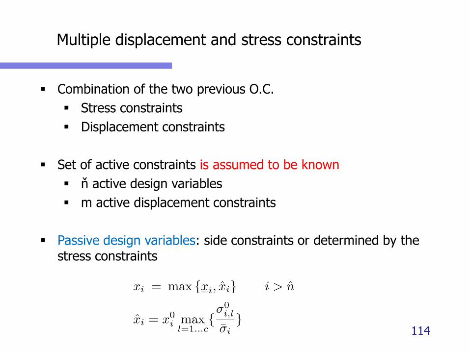
▪ Combination of the two previous O.C.
▪ Stress constraints
▪ Displacement constraints
▪ Set of active constraints is assumed to be known
▪ ň active design variables
▪ m active displacement constraints
▪ Passive design variables: side constraints or determined by the stress constraints
114

Multiple displacement and stress constraints
▪ Active variables ➔ optimality conditions w.r.t. displacement
constraints (assumed to be active)
▪ Lagrange function
▪ ➔ m Lagrange multipliers j
▪ Explicit approximation using virtual work
115
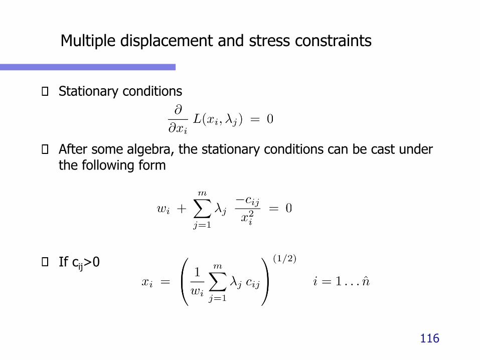
Multiple displacement and stress constraints
Stationary conditions
After some algebra, the stationary conditions can be cast under the following form
If cij>0
116

Multiple displacement and stress constraints
▪ After some algebra, the stationary conditions can be rewritten under the following form
▪ With the virtual (mutual) strain energy densities
▪ In optimized structure, we have in each element the same combined virtual energy density, equal to unity
117
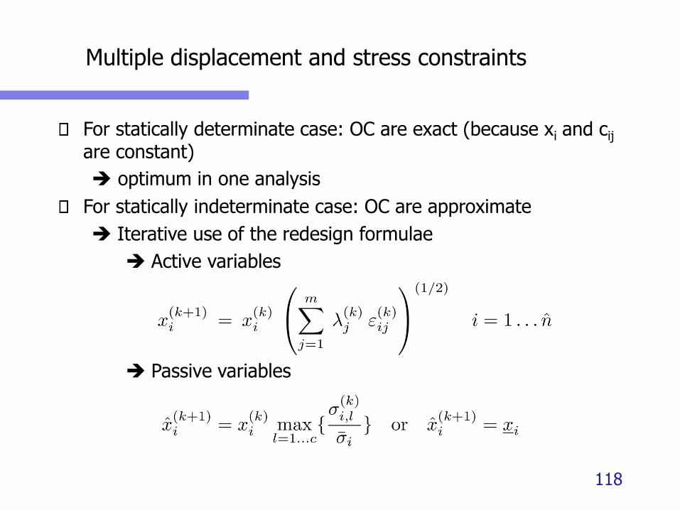
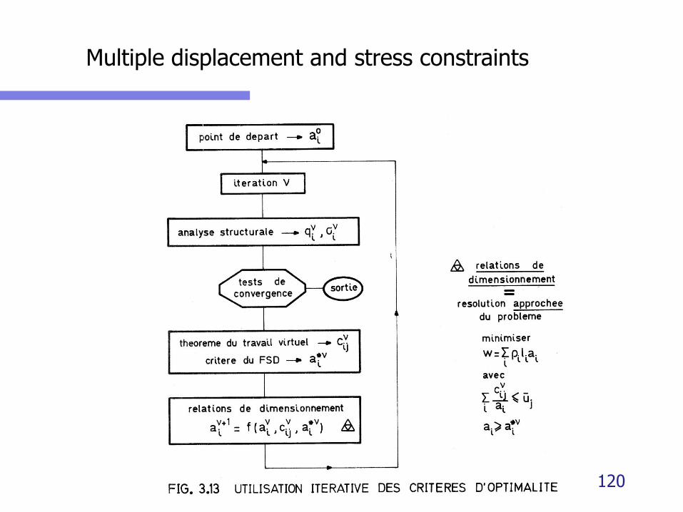
Multiple displacement and stress constraints
For statically determinate case: OC are exact (because xi and cij
are constant)
➔ optimum in one analysis
For statically indeterminate case: OC are approximate
➔ Iterative use of the redesign formulae
➔ Active variables
➔ Passive variables
118
Multiple displacement and stress constraints
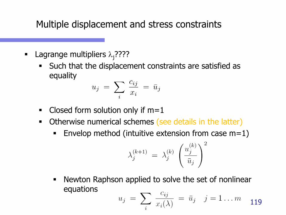
▪ Lagrange multipliers j????
▪ Such that the displacement constraints are satisfied as equality
▪ Closed form solution only if m=1
▪ Otherwise numerical schemes (see details in the latter)
▪ Envelop method (intuitive extension from case m=1)
▪ Newton Raphson applied to solve the set of nonlinear equations
119
Multiple displacement and stress constraints
120

Envelop method (Gellatly & Berke, 1971)
▪ Intuitive method, simple use, close to FSD
▪ Each displacement constraint is first considered alone and independently.
▪ For constraint j only
▪ and
▪ Then, one takes the maximum size for all displacement constraints (envelop)
121
Envelop method (Gellatly & Berke, 1971)
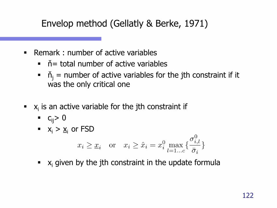
▪ Remark : number of active variables
▪ ň= total number of active variables
▪ ňj = number of active variables for the jth constraint if it was the only critical one
▪ xi is an active variable for the jth constraint if
▪ cij> 0
▪ xi > xi or FSD
▪ xi given by the jth constraint in the update formula
122
Envelop method (Gellatly & Berke, 1971)
▪ Formula must be repeated 2 or 3 times before stabilizing the sets of active design variables for each constraint
▪ The approach produces satisfactory results if the number of constraints is not too large
▪ Advantages
▪ Easy implementation
▪ No numerical difficulties
123
Newton-Raphson iteration (Taig & Kerr, 1973)
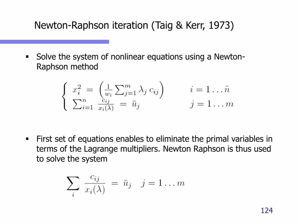
▪ Solve the system of nonlinear equations using a Newton-Raphson method
▪ First set of equations enables to eliminate the primal variables in terms of the Lagrange multipliers. Newton Raphson is thus used to solve the system
124
Newton-Raphson iteration (Taig & Kerr, 1973)
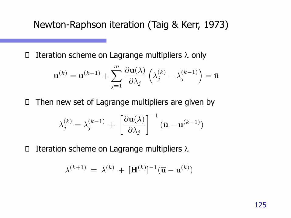
Iteration scheme on Lagrange multipliers only
Then new set of Lagrange multipliers are given by
Iteration scheme on Lagrange multipliers
125
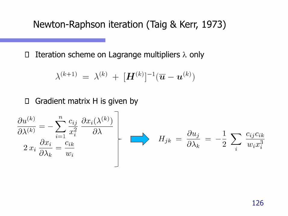
Newton-Raphson iteration (Taig & Kerr, 1973)
Iteration scheme on Lagrange multipliers only
Gradient matrix H is given by
126

Newton-Raphson iteration (Taig & Kerr, 1973)
▪ Difficulties
▪ Select appropriate initial (0)
▪ Find the correct set of active / passive design variables
▪ Identify the set of estimated active behaviour constraints (i.e. nonzero j’s)
▪ H might become singular at some stage of the process
▪ Solution: dual methods
▪ H is indeed the Hessian matrix of the dual function
▪ Iteration is the quadratic programming ascent direction in dual space
127

Ten-bar-truss example
▪ The stress-ratioïng itself tends to increase the design variable with the smallest stress limit
▪ Example: stress limit = 25000psi except in member 8 with a variable limit from 25000 to 70000 psi
128
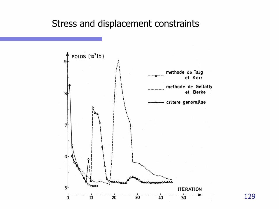
Stress and displacement constraints
129