recent attempts in the analysis of black hole radiation
TRANSCRIPT

arX
iv:1
003.
5534
v1 [
hep-
th]
29
Mar
201
0
Recent Attempts in the Analysisof Black Hole Radiation
Koichiro Umetsu 1
Graduate School of Quantum Science and Technology,Nihon University, Tokyo 101-8308, Japan
January, 2010
A Dissertation in candidacy for the degreeof Doctor of Philosophy
1E-mail: [email protected]


Abstract
In this thesis, we first present a brief review of black hole radiation which is commonly calledHawking radiation. The existence of Hawking radiation by itself is well established by now becausethe same result is derived by several different methods. On the other hand, there remain severalaspects of the effect which have yet to be clarified. We clarify some arguments in previous workson the subject and then attempt to present the more satisfactory derivations of Hawking radiation.To be specific, we examine the analyses in the two recent derivations of Hawking radiation whichare based on anomalies and tunneling; both of these derivations were initiated by Wilczek and hiscollaborators. We then present a simple derivation based on anomalies by emphasizing a systematicuse of covariant currents and covariant anomalies combined with boundary conditions which haveclear physical meaning. We also extend a variant of the tunneling method proposed by Banerjeeand Majhi to a Kerr-Newman black hole by using the technique of the dimensional reduction nearthe horizon. We directly derive the black body spectrum for a Kerr-Newman black hole on thebasis of the tunneling mechanism.
i

ii

Contents
1 Introduction 1
2 Properties of Black Hole 5
2.1 General Theory of Relativity and Black Hole . . . . . . . . . . . . . . . . . . . . . 5
2.2 Penrose Diagram . . . . . . . . . . . . . . . . . . . . . . . . . . . . . . . . . . . . . 10
2.3 Energy Extraction from Rotating Black Holes . . . . . . . . . . . . . . . . . . . . . 18
2.3.1 Penrose process . . . . . . . . . . . . . . . . . . . . . . . . . . . . . . . . . . 18
2.3.2 Superradiance . . . . . . . . . . . . . . . . . . . . . . . . . . . . . . . . . . . 22
2.4 Dimensional Reduction near the Horizon . . . . . . . . . . . . . . . . . . . . . . . . 26
2.5 Analogies between Black Hole Physics and Thermodynamics . . . . . . . . . . . . 29
2.6 Black Holes and Entropy . . . . . . . . . . . . . . . . . . . . . . . . . . . . . . . . . 34
2.6.1 Entropy in information theory . . . . . . . . . . . . . . . . . . . . . . . . . 35
2.6.2 The minimum increase of the black hole area . . . . . . . . . . . . . . . . . 36
2.6.3 Information loss and black hole entropy . . . . . . . . . . . . . . . . . . . . 40
3 Black Hole Radiation 45
3.1 Hawking’s Original Derivation . . . . . . . . . . . . . . . . . . . . . . . . . . . . . . 46
3.2 Previous Works on Hawking Radiation . . . . . . . . . . . . . . . . . . . . . . . . . 59
4 Hawking Radiation and Anomalies 65
4.1 Quantum Anomaly . . . . . . . . . . . . . . . . . . . . . . . . . . . . . . . . . . . . 65
4.2 Derivation of Hawking Radiation from Anomalies . . . . . . . . . . . . . . . . . . . 69
4.3 Ward Identity in the Derivation of Hawking Radiation from Anomalies . . . . . . . 72
iii

4.3.1 The case of a Kerr black hole . . . . . . . . . . . . . . . . . . . . . . . . . . 72
4.3.2 Comparison with previous works . . . . . . . . . . . . . . . . . . . . . . . . 77
4.3.3 The case of a Reissner-Nordstrom black hole . . . . . . . . . . . . . . . . . 82
5 Hawking Radiation and Tunneling Mechanism 87
5.1 Hawking Radiation as Tunneling . . . . . . . . . . . . . . . . . . . . . . . . . . . . 89
5.2 Tunneling Mechanism in the Canonical Theory . . . . . . . . . . . . . . . . . . . . 93
5.3 Hawking Black Body Spectrum from Tunneling Mechanism . . . . . . . . . . . . . 96
5.4 Hawking Radiation from Kerr-Newman Black Hole and Tunneling Mechanism . . . 103
5.4.1 Kruskal-like coordinates for the effective 2-dimensional metric . . . . . . . . 104
5.4.2 Tunneling mechanism . . . . . . . . . . . . . . . . . . . . . . . . . . . . . . 108
5.4.3 Black body spectrum and Hawking flux . . . . . . . . . . . . . . . . . . . . 112
6 Discussion and Conclusion 117
Appendix . . . . . . . . . . . . . . . . . . . . . . . . . . . . . . . . . . . . . . . . . . . . 121
A Killing Vectors and Null Hypersurfaces . . . . . . . . . . . . . . . . . . . . . . . . . 121
B The First Integral by Carter . . . . . . . . . . . . . . . . . . . . . . . . . . . . . . . 123
C Bogoliubov Transformations . . . . . . . . . . . . . . . . . . . . . . . . . . . . . . . 126
D Solutions of Klein-Gordon Equation in Schwarzschild Space-time . . . . . . . . . . 127
E Calculation of Bogoliubov Coefficients . . . . . . . . . . . . . . . . . . . . . . . . . 133
iv

Chapter 1
Introduction
General theory of relativity and quantum theory are two fundamental theories in modern
physics. According to the current understanding of physics, it is well known that all the forces
which have been identified in nature can be explained by the electromagnetic force, weak force,
strong force and gravity. The first three of them are described by quantum field theory and the
remaining gravity is described by the general theory of relativity.
Furthermore, the idea of a unified field theory, which can describe the four forces by a single
theory, was advanced. Electromagnetic and weak forces were unified byWeinberg-Salam theory and
a grand unified theory which combines the strong interaction with the electroweak interactions was
proposed. However, gravity has yet to be successfully included in a theory of everything. A simple
attempt to combine the gravitational interaction with the strong and electroweak interactions
runs into fundamental difficulties since the resulting theory is not renormalizable. This means
that physically meaningful observables contain nonremovable infinities. The string theory has
potentiality which solves these problems. However, we have not obtained any solid result in string
theory yet and it depends on the future progress. We have not yet formulated a widely accepted,
consistent theory that combines the general theory of relativity with the principle of quantum
theory. In any case, we must study a framework where both of the general theory of relativity and
quantum theory are consistently incorporated.
From the above point of view, the black hole radiation which was suggested by Hawking is
very interesting. Although we have not yet confirmed that black holes do really exist, it has been
predicted that they exist as a consequence of the general theory of relativity, namely, as special
solutions of the basic Einstein equation. According to the Einstein equation, the space-time is
curved by the effects of gravity. The space-time curved by a very strong gravity can form a closed
1

region from which nothing, not even photons, can escape. The closed region is the black hole.
Thus black holes cannot classically allow the emission of radiation. However, by using quantum
field theory in black hole physics, a mechanism by which black holes can radiate was proposed
by Hawking [1, 2]. The radiation from the black hole is commonly called the Hawking radiation.
In this sense, it can be said that Hawking radiation is one of precious phenomena where both of
the general theory of relativity and quantum theory play a role at the same time. When any new
theory of quantum gravity is constructed, it must be checked if it correctly describes Hawking
radiation in the proposed theory.
Hawking’s original derivation is very direct and physical [2]. The analysis calculates the Bo-
goliubov coefficients between the in- and out-states for a body collapsing to form a black hole.
It is well-known that the characteristic spectrum found in the original derivation agrees with the
black body spectrum with a characteristic temperature associated with the black hole if we ignore
the back scattering of particles falling into the black hole. Namely, it was found that a black hole
behaves as a black body and the black hole emits radiation.
After Hawking’s original derivation, various derivations of Hawking radiation have been sug-
gested. All of them reproduce the same result that the black hole entropy is described by the
surface area of the black hole and the temperature of the black hole is described by a surface grav-
ity of the black hole. Hawking radiation is thus one of the most striking effects which are widely
accepted by now. However, there are several aspects which have not been completely clarified yet.
In particular, although the entropy is interpreted as a count of the number of states in statistical
mechanics, the entropy of a black hole with a finite temperature has not been derived by counting
the number of quantum states associated with the black hole. It is considered that this problem
is closely related to the fact that quantum theory of gravity has not been explicitly formulated
yet, and it is very difficult to construct a consistent quantum gravity. By examining the various
derivations of Hawking radiation, we find that each derivation has both merits and demerits. In
this sense, it may be fair to say that these known derivations of Hawking radiation have not reached
an impeccable conclusion yet.
Recently, Robinson and Wilczek suggested a new method of deriving Hawking radiation by the
consideration of anomalies [3]. The basic idea of the approach is that the flux of Hawking radiation
is determined by anomaly cancellation conditions in the background of a Schwarzschild black hole.
Iso, Umetsu and Wilczek improved the approach by Robinson and Wilczek, and they extended
the method to a charged black hole [4] and a rotating black hole [5]. The approach of Iso, Umetsu
2

and Wilczek [5] is very transparent and interesting. However, there remain several points to be
clarified. We have presented arguments which clarify the basic idea of the derivation and given
a simple derivation by using the Ward Identities and boundary conditions [6]. We would like to
explain our simple derivation as comprehensibly as possible in the present thesis.
A straightforward derivation on the basis of the tunneling mechanism was also suggested by
Parikh and Wilczek [7]. The analysis of tunneling mechanism was mainly confined to the derivation
of the temperature of a black hole, and the black body spectrum itself has not been much discussed.
More recently, this problem of the black body spectrum was emphasized by Banerjee and Majhi [8].
They showed how to reproduce the black body spectrum directly, which agrees with Hawking’s
original result, by using the properties of the tunneling mechanism. Thus the derivation on the
basis of the tunneling mechanism became more satisfactory. Their result is valid only for black
holes with a spherically symmetric geometry. However, it is known that 4-dimensional black holes
have not only a mass and a charge but also angular momentum, and the geometry of a rotating
black hole becomes spherically asymmetric because of its own rotation. We have recently attempted
to extend Banerjee and Majhi’s method to a rotating black hole by using a technique valid only
near the horizon, which is called the dimensional reduction [9]. We showed that the result agrees
with the previous result. We explain our method which shows how to directly derive the black
body spectrum for a rotating black hole on the basis of the tunneling mechanism in this thesis.
To the best of my knowledge, there is no derivation of the spectrum by using the technique of
the dimensional reduction in the tunneling mechanism. Therefore, we believe that this derivation
clarifies some aspects of the tunneling mechanism.
The contents of the present thesis are as follows. In Chapter 2, we review some properties of
black holes. These properties will be useful to understand the contents of the following chapters.
In Chapter 3, we review the original derivation of Hawking radiation by Hawking and briefly
explain other representative derivations of Hawking radiation. It will be argued that there are
several aspects to be clarified in the existing derivations of Hawking radiation. In Chapter 4,
we discussed the derivation of Hawking radiation which is based on anomalies. We clarify some
aspects in previous works on this subject and present a simple derivation of Hawking radiation
from anomalies. In Chapter 5, we discussed the derivation of Hawking radiation which is based
on quantum tunneling. We present a generalization of the derivation of Hawking radiation by
Banerjee and Majhi on the basis of the tunneling mechanism to a rotating black hole and also
give some clarifying comments. Chapter 6 is devoted to discussion and conclusion. Some of the
3

technical details are given in appendices.
In this paper, we use the natural system of units
c = G = ~ = 1 (1.0.1)
unless stated otherwise, where c is the speed of light in vacuum, G is the gravitational constant
and ~ is the Planck constant (Dirac’s constant).
4

Chapter 2
Properties of Black Hole
The existence of black holes has been predicted by the general theory of relativity. To under-
stand Hawking radiation, we have to know some classical properties of black holes first. In this
chapter we would like to review some properties of black holes.
The contents of this chapter are as follows. In Section 2.1, we review the general theory of
relativity and black holes. We would also like to mention various types of black holes. In Section
2.2, we refer to the Penrose diagram and show how to describe it. In Section 2.3, we discuss how
to extract energy from a rotating black hole classically. In Section 2.4, we would like to discuss the
dimensional reduction near the event horizon which is a boundary between our universe and a black
hole. By using the technique of the dimensional reduction, we show that a 4-dimensional metric
associated with a charged and rotating black hole effectively becomes a 2-dimensional spherically
symmetric metric. In Section 2.5, we would like to discuss analogies between black hole physics
and thermodynamics. In Section 2.6, we review the argument, which was suggested by Bekenstein,
that black holes have entropy. These introductory discussions will be useful to understand the
contents of the following chapters.
2.1 General Theory of Relativity and Black Hole
General theory of relativity is the theory of space-time and gravitation formulated by Einstein
in 1915 [10]. The Einstein equation which describes the general theory of relativity is given by [11]
Rµν − 1
2Rgµν =
8πG
c4Tµν , (2.1.1)
where Rµν is the Ricci tensor, R is the Ricci scalar, gµν is the metric of space-time, G is the
gravitational constant, c is the speed of light, and Tµν is the energy-momentum tensor. These
5

quantities are defined by
R ≡ Rµµ = gµνRνµ (2.1.2)
Rµν ≡ Rρµνρ (2.1.3)
Rρµνσ ≡ ∂νΓ
ρµσ − ∂σΓ
ρµν + Γα
µσΓραν − Γα
µνΓρασ (2.1.4)
Γρµν ≡ 1
2gρα (∂νgαµ + ∂µgαν − ∂αgµν) (2.1.5)
ds2 ≡ gµνdxµdxν , (2.1.6)
where Rρµνσ is the Riemann-Christoffel tensor or the curvature tensor, Γρ
µν is the Christoffel symbol,
and ds is the line element. The expression on the left-hand side of the equation (2.1.1) represents
the curvature of space-time as determined by the metric, and the expression on the right-hand side
represents the distribution of matter fields. The Einstein equation is then interpreted as a set of
equations dictating how the curvature of space-time is related to the distribution of matter and
energy in the universe.
It is difficult to solve the general solution for the Einstein equation because the Einstein equation
is the quadratic nonlinear differential equation. However, it is known that there are several exact
solutions for the Einstein equation. In 1916, Schwarzshild found an exact solution for the Einstein
equation [12] which describes the gravitational field outside a black hole which depends only on
the mass.
It is considered that black holes are formed as a result of the gravitational collapse of a star
with a very large mass. The original stars which will form the black hole have various physical
quantities and properties. As soon as a black hole is formed by the gravitational collapse, the state
of the black hole becomes a stationary state. It is known that the stationary state is characterized
by only three physical parameters, namely, the mass, the angular momentum and the electrical
charge. This means that a black hole does not retain the various information of the original
star except for these three parameters. In other words, a black hole can uniquely be decided
by the mass, the angular momentum and the charge. This consequence is called the black hole
uniqueness theorem [13–15] or the no-hair theorem [16], and the uniqueness theorem is shown in a
4-dimensional theory if the solutions of the Einstein equation satisfy the four conditions
1. Only electromagnetic field exits.
2. Asymptotically flat.
3. Stationary.
4. No singularity exists on and outside the event horizon.
6

Here the fourth condition is based on the cosmic censorship hypothesis proposed by Penrose [17].
Black holes are divided into four groups by depending on parameters and each has its own
name (Tab. 2.1). The Schwarzschild black hole depends on only the mass. The Schwarzschild
metric, which describes the space-time outside the Schwarzschild black hole, is given by
ds2 = −(
1− 2M
r
)
dt2 +1
1− 2Mr
dr2 + r2dθ2 + r2 sin2 θdϕ2, (2.1.7)
where r, θ and ϕ are commonly used variables in polar coordinates, andM is the mass of the black
hole. The Reissner-Nordstrom black hole depends on both the mass and the charge. The Kerr
black hole depends on both the mass and the angular momentum. The Kerr-Newman black hole
depends on the mass, the charge and the angular momentum. The Kerr-Newman metric is given
by
ds2 =− ∆− a2 sin2 θ
Σdt2 − 2a sin2 θ
Σ(r2 + a2 −∆)dtdϕ
− a2∆sin2 θ − (r2 + a2)2
Σsin2 θdϕ2 +
Σ
∆dr2 +Σdθ2, (2.1.8)
where a is defined in order to adjust the dimensions by
a ≡ L
M, (2.1.9)
and for simplicity, the symbols are respectively defined by
Σ ≡ r2 + a2 cos2 θ, (2.1.10)
∆ ≡ r2 − 2Mr + a2 +Q2. (2.1.11)
In 4 dimensions, the Kerr-Newman black hole is the most general black hole. We can thus obtain
the Kerr metric by taking Q = 0 in the metric (2.1.8), and we also obtain the Reissner-Nordstrom
metric by taking L = 0, namely, a = 0. Of course, by taking both Q = 0 and a = 0 in (2.1.8), it
can be checked that the Kerr-Newman metric (2.1.8) actually becomes the Schwarzschild metric
(2.1.7). We also note that the metric (2.1.8) is asymptotically flat, i.e., it approaches the Minkowski
metric
ds2 = ηµνdxµdxν = −dt2 + dx2 + dy2 + dz2. (2.1.12)
which stands for the flat space-time in our universe.
7
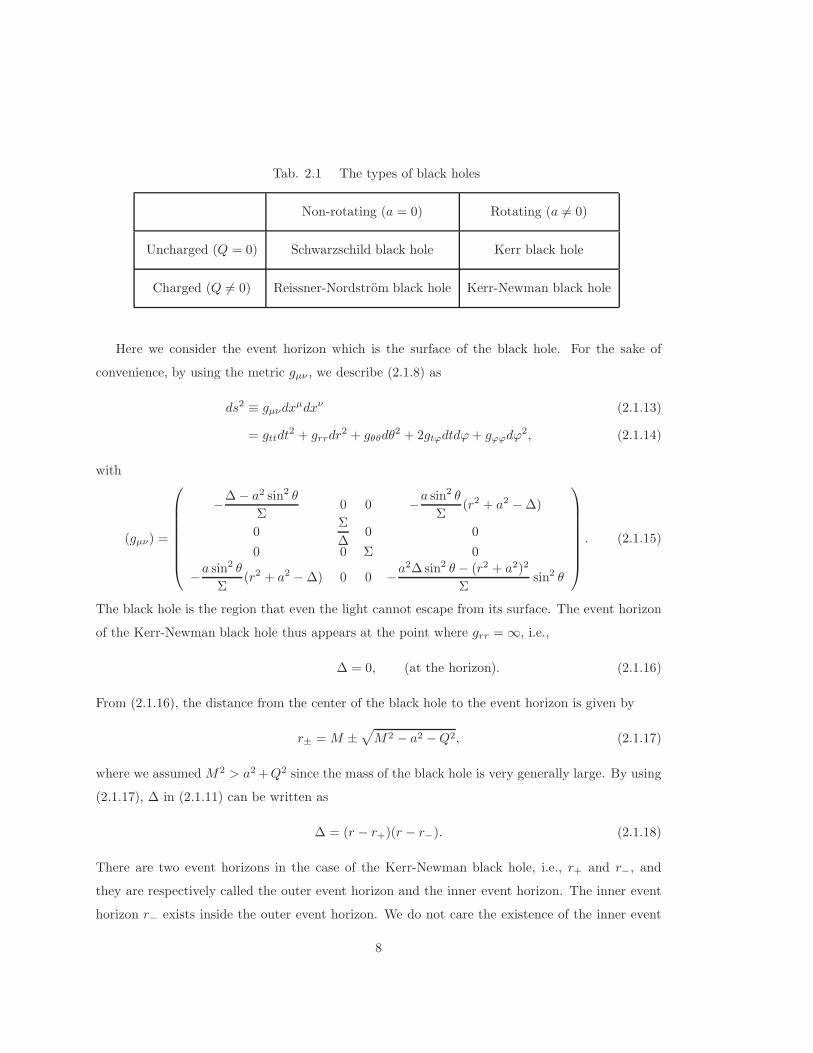
Tab. 2.1 The types of black holes
Non-rotating (a = 0) Rotating (a 6= 0)
Uncharged (Q = 0) Schwarzschild black hole Kerr black hole
Charged (Q 6= 0) Reissner-Nordstrom black hole Kerr-Newman black hole
Here we consider the event horizon which is the surface of the black hole. For the sake of
convenience, by using the metric gµν , we describe (2.1.8) as
ds2 ≡ gµνdxµdxν (2.1.13)
= gttdt2 + grrdr
2 + gθθdθ2 + 2gtϕdtdϕ+ gϕϕdϕ
2, (2.1.14)
with
(gµν) =
−∆− a2 sin2 θ
Σ0 0 −a sin
2 θ
Σ(r2 + a2 −∆)
0Σ
∆0 0
0 0 Σ 0
−a sin2 θ
Σ(r2 + a2 −∆) 0 0 −a
2∆sin2 θ − (r2 + a2)2
Σsin2 θ
. (2.1.15)
The black hole is the region that even the light cannot escape from its surface. The event horizon
of the Kerr-Newman black hole thus appears at the point where grr = ∞, i.e.,
∆ = 0, (at the horizon). (2.1.16)
From (2.1.16), the distance from the center of the black hole to the event horizon is given by
r± =M ±√
M2 − a2 −Q2, (2.1.17)
where we assumed M2 > a2+Q2 since the mass of the black hole is very generally large. By using
(2.1.17), ∆ in (2.1.11) can be written as
∆ = (r − r+)(r − r−). (2.1.18)
There are two event horizons in the case of the Kerr-Newman black hole, i.e., r+ and r−, and
they are respectively called the outer event horizon and the inner event horizon. The inner event
horizon r− exists inside the outer event horizon. We do not care the existence of the inner event
8

horizon since we cannot know information inside the outer horizon. In what follows, we simply
describe the outer event horizon as the horizon.
On the horizon r = r+, the metric (2.1.8) becomes the intrinsic metric given by
ds2 = −a2∆+ sin2 θ − (r2+ + a2)2
Σ+sin2 θdϕ2 +Σ+dθ
2, (2.1.19)
since both t and r are constant on the horizon, i.e., dt = dr = 0. Here we defined ∆+ ≡ ∆(r+) = 0
and Σ+ ≡ Σ(r+). We thus find that the area of the black hole A is given by
A =
∫
√
gθθ(r+)gϕϕ(r+)dθdϕ = 4π(r2+ + a2). (2.1.20)
From ∆+ = r2+ − 2Mr+ + a2 +Q2 = 0, we can also write the black hole area as
A = 4π(2Mr+ −Q2). (2.1.21)
By taking the total differentiation of (2.1.21), we obtain
dM =κ
8πdA+ΩHdL+ΦHdQ, (2.1.22)
where κ, ΩH and ΦH are respectively the surface gravity, the angular velocity and the electrical
potential on the horizon, which are defined by
κ ≡ 4π(r+ −M)
A, (2.1.23)
ΩH ≡ 4πa
A, (2.1.24)
ΦH ≡ 4πr+Q
A. (2.1.25)
It is known that the relation (2.1.22) is the energy conservation law in black hole physics. It is
easy to find that the each term has the dimension of the energy in the natural system of units.
Before closing this section, we would like to state black holes in various dimensions. It is
known that a vacuum solution of the Einstein equation without the cosmological constant in three
dimensions ((2+1)-dimensions), corresponds to a flat solution and no black hole solution exists.
However, when we consider the Einstein equation with a negative cosmological constant which
behaves as attraction, we can obtain black hole solutions in 3-dimensions. It is called the BTZ
black hole, which was found by Banados, Teitelboim and Zanelli [19,57]. It is known that it is the
lowest dimensional black hole.
In dimensions higher than four, there are several black hole solutions because the restriction
of topology with respect to the horizon is alleviated. Therefore, a black hole cannot be uniquely
9

decided even if the mass, the angular momentum and the charge are given. This suggests that the
uniqueness theorem is not satisfied. For example, in five dimensions, there are the Myers-Perry
black hole which has two independent rotation parameters [20] and the black ring [21]. We thus
have these two solutions with the same mass and the same angular momenta. It is thus known
that the black hole uniqueness theorem does not hold in the higher dimensional theory.
2.2 Penrose Diagram
Penrose diagram is very useful to understand the global structure of black hole space-time. It
was proposed by Penrose in 1964 [22]. In this section, we would like to recall the advantages of
using the Penrose diagram. Then we will show how to describe the Penrose diagram.
For simplicity, we consider the case of the Schwarzschild black hole. The Schwarzschild metric
is given by
ds2 = −(
1− 2M
r
)
dt2 +1
1− 2Mr
dr2 + r2dΩ2, (2.2.1)
where dΩ2 stands for a 2-dimensional unit sphere defined by
dΩ2 ≡ dθ2 + sin2 θdϕ2. (2.2.2)
It follows from the expression (2.2.1) that there are two singularities r = 0 and r = 2M in
the Schwarzschild metric. A singularity at r = 0 is the curvature singularity which cannot be
removed while the other at r = 2M is a fictitious singularity arising merely from an improper
choice of coordinates. We therefore know that the singularity at r = 2M can be removed by using
appropriate coordinates.
The Penrose diagram is drawn for the Schwarzschild metric as in Fig. 2.1. The notations I0,
I± and J ± appearing in Fig. 2.1, respectively stand for the following regions
I0 =
t ; finiter → ∞ ,
I± =
t→ ±∞r ; finite ,
(2.2.3)
J − =
t → −∞r → +∞ ,
J + =
t→ +∞r → +∞ ,
(2.2.4)
and two double lines of R stand for the curvature singularity of the Schwarzschild metric. The
heavy lines H+ and H− also stand for
H+ =
t → +∞r = 2M ,
H− =
t→ −∞r = 2M ,
(2.2.5)
and H+ and H− are respectively called the future event horizon and the past event horizon.
10

I0
I+
I−
R
J +
J −
H+H−
r = const.
Fig. 2.1 The Penrose diagram for the Schwarzschild solution.
We can draw the Penrose diagram through some coordinate transformations (see, for example,
[23]). As a first step of coordinate transformations, we use the tortoise coordinate defined by [24,25]
dr∗ ≡ 1
1− 2Mr
dr. (2.2.6)
The metric (2.2.1) is then written by
ds2 = −(
1− 2M
r
)
(dt− dr∗)(dt+ dr∗) + r2dΩ2. (2.2.7)
By integrating (2.2.6) over r from 0 to r, we obtain
r∗ = r + 2M ln∣
∣
∣
r
2M− 1∣
∣
∣ . (2.2.8)
As the second step we use the Eddington-Finkelstein coordinates defined by [26, 27]
v ≡ t+ r∗ = t+ r + 2M ln∣
∣
∣
r
2M− 1∣
∣
∣ ,
u ≡ t− r∗ = t− r − 2M ln∣
∣
∣
r
2M− 1∣
∣
∣ ,(2.2.9)
where v is called the advanced time and u is called the retarded time. The metric (2.2.7) is then
written as
ds2 = −(
1− 2M
r
)
dvdu + r2dΩ2. (2.2.10)
11

As the third step we use the Kruskal-Szekeres coordinates [28, 29]. When r > 2M , these
coordinates are defined by
V ≡ exp[ v
4M
]
,
U ≡ − exp[
− u
4M
]
,(2.2.11)
and the metric (2.2.10) is written as
ds2 = −32M3
rexp
[
− r
2M
]
dV dU + r2dΩ2, when r > 2M. (2.2.12)
When r < 2M , these coordinates are defined by
V ≡ exp[ v
4M
]
,
U ≡ exp[
− u
4M
]
,(2.2.13)
and the metric (2.2.10) is then written as
ds2 =32M3
rexp
[
− r
2M
]
dV dU + r2dΩ2, when r < 2M. (2.2.14)
As the fourth step we use the following coordinate transformations defined by
V = tan−1
(
V
4M√2M
)
,
U = tan−1
(
U
4M√2M
)
.
(2.2.15)
We find that infinities appeared in V or U are converted to finite values such asπ
2or −π
2.
As the final step we use the following coordinate transformations defined by
T =1
2
(
V + U)
,
R =1
2
(
V − U)
.
(2.2.16)
Penrose diagram is drawn by choosing the vertical axis as T and the horizontal axis as R.
As an illustration, we draw I+ and J+. First, I+ is expressed by
I+ =
t→ +∞r ; finite .
(2.2.17)
Since r is finite, we need to consider two cases of r > 2M and r < 2M . When r > 2M , by
substituting (2.2.17) into (2.2.9), v and u become
I+ =
v → +∞u→ +∞ .
(2.2.18)
12

While when r < 2M , by substituting (2.2.17) into (2.2.13), v and u agree with (2.2.18). By
substituting (2.2.18) into (2.2.11), V and U become
I+ =
V → +∞U → 0 ,
(2.2.19)
and by substituting (2.2.19) into (2.2.15), V and U become
I+ =
V → +π
2U → 0 .
(2.2.20)
By substituting (2.2.20) into (2.2.16), T and R become
I+ =
T → +π
4
R → +π
4.
(2.2.21)
We thus find that the region I+ as in (2.2.17) is represented by (R, T ) =(π
4,π
4
)
in the Penrose
diagram, when r takes finite values except r = 2M (Fig. 2.2).
I+
T
0R
π4
π4
(π4 ,π4 )
Fig. 2.2 The region of I+ in the Penrose diagram.
Next, we similarly draw J+. The region J + is expressed by
J+ =
t→ +∞r → +∞u ; finite .
(2.2.22)
Since r is at infinity, we have only to consider the case of r > 2M . By substituting (2.2.22) into
(2.2.9), v and u become
J + =
v → +∞u ; finite .
(2.2.23)
13

By substituting (2.2.23) into (2.2.11), V and U become
J+ =
V → +∞U ; finite ,
(2.2.24)
and by substituting (2.2.24) into (2.2.15), V and U become
J + =
V → +π
2U ; finite .
(2.2.25)
Finally, by substituting (2.2.25) into (2.2.16), T and R become
J + =
T =1
2
(π
2+ U
)
R =1
2
(π
2− U
)
.
(2.2.26)
From these two relations (2.2.26), we thus find that the region J + as in (2.2.22) is represented by
the segment of a line
T =π
2− R (2.2.27)
in the Penrose diagram (Fig. 2.3).
J+
T
0R
(π4 ,π4 )
π4
π4
π2
π2
Fig. 2.3 The region of J+ in the Penrose diagram.
We can similarly draw other points and segments (Tab. 2.2). In Tab. 2.2, when a variable is
finite and is not uniquely fixed, the name of the variable is retained. The diagram drawn by using
14

Tab. 2.2, is expressed as in Fig. 2.4. The regions R+ and R− respectively stand for the following
regions
R+ =
t→ +∞r = 0 ,
R− =
t→ −∞r = 0 ,
(2.2.28)
and the double line R combines between R+ and R−. The region R stands for r = 0 with finite
t, but we cannot uniquely decide the point in the region R. This means that we do not know how
to draw an exact line of the region R. We therefore drew a double line as the line R. Also by
comparison with Fig. 2.1, there are some missing parts in Fig. 2.4. We can draw them by defining
the other universe where time proceeds reversely by comparison with our universe. We however
skip them because they are not important in the body of the present thesis.
Tab. 2.2 Coordinate values in each region
Region (t, r) (v, u) (V, U)(
V , U) (
T , R)
I+ (+∞, r) (+∞,+∞) (+∞, 0)(
+π
2, 0) (
+π
4,+
π
4
)
I− (−∞, r) (−∞,−∞) (0,−∞)(
0,−π2
) (
−π4,+
π
4
)
I0 (t,+∞) (+∞,−∞) (+∞,−∞)(
+π
2,−π
2
) (
0,+π
2
)
J + (+∞,+∞) (+∞, u) (+∞, U)(π
2, U)
T =π
2− R
J − (−∞,+∞) (v,−∞) (V,−∞)(
V ,−π2
)
T = R− π
2
H+ (+∞, 2M) (v,+∞) (V, 0)(
V , 0)
T = R
H− (−∞, 2M) (−∞, u) (0, U)(
0, U)
T = −R
R+ (+∞, 0) (+∞,+∞) (+∞, 0)(
+π
2, 0) (
+π
4,+
π
4
)
R− (−∞, 0) (−∞,−∞) (0,∞)(
0,+π
2
) (
+π
4,−π
4
)
15

I0
I+
I−
R
J +
J−
H+H−
T
R
R+R−
Fig. 2.4 The Penrose diagram corresponding to Tab. 2.1.
As above, the Penrose diagram can represent infinite time or radial coordinates as points or
lines. In this diagram null geodesics is also represented as lines of ±45 to the vertical. Each point
of the diagram represents a 2-dimensional sphere of area 4πr2. Namely, angular coordinates θ and
ϕ as in (2.2.1) are attached to each point of the coordinate. For this reason, the Penrose diagram
is also called the conformal diagram.
The Penrose diagram is divided into four regions by the two diagonal lines H+ and H− (Fig.
2.5). The region I represents our universe. The region II represents a black hole. The region III
represents the other universe that time reversely proceeds by comparison with our universe. The
region IV represents a white hole which is the time reversal of a black hole and ejects matter from
the horizon. For example, we find that null geodesics in the region I can arrive at J+ or the black
hole through the horizon H+ but null geodesics in the region II (inside the black hole) cannot arrive
at our universe through the horizon H+.
16

I0
I+
I−
r = 0
J +
J −
H+H−
II
IIII
IV
Fig. 2.5 The Penrose diagram for the Schwarzschild solution.
Now we consider that a black hole is formed by the gravitational collapse of a star with a
heavy mass. This was comprehensibly discussed by Hawking in the literature [2]. Hence we would
faithfully like to present the argument by following Hawking’s exposition. For simplicity, we assume
that the gravitational collapse is spherically symmetric. Such a object starts to collapse at the
point I−. Since the collapsing object has a mass, the passing is later than light (Fig. 2.6). In Fig.
2.6, the time-like geodesic with an angle, which is smaller than 45, represents the surface of the
collapsing object and the shaded region represents inside the collapsing object.
I0
I+
I−
r = 0
J +
J −
Fig. 2.6 The development of the collapsing object in the Penrose diagram.
In the case of exactly spherical collapse, the metric is exactly the Schwarzschild metric every-
where outside the surface of the collapsing object. O the other hand, inside the object the metric
17

is completely different. Thus, the past event horizon, the past curvature singularity and the other
asymptotically flat region do not exist and are replaced by a time-like curve representing the origin
of polar coordinates. The appropriate Penrose diagram is shown in Fig. 2.7. We represented the
origin as the vertical dotted line because the metric inside the object might be nonsingular at the
origin.
singularity
J +
J−
I−
r = 0
H+
origin ofcoordinate
Fig. 2.7 The Penrose diagram of a spherically symmetric
collapsing body producing a black hole.
2.3 Energy Extraction from Rotating Black Holes
By definition, a black hole is a “region of no escape.” It might thus seem that energy cannot be
extracted from a black hole. However, the mechanism of energy extraction from a rotating black
hole was proposed by Penrose [30]. The process is called the Penrose process and the radiance is
called the black hole superradiance. This can be explained in the classical theory.
2.3.1 Penrose process
In this subsection, we would like to show how to extract energy from a rotating black hole. To
begin with, we shall present an intuitive explanation. The metric of a rotating black hole is given
18
by the Kerr metric
ds2 =− ∆− a2 sin2 θ
Σdt2 − 2a sin2 θ
Σ(r2 + a2 −∆)dtdϕ
− a2∆sin2 θ − (r2 + a2)2
Σsin2 θdϕ2 +
Σ
∆dr2 +Σdθ2. (2.3.1)
This form agrees with the Kerr-Newman metric (2.1.8) but the contents of both ∆ and Σ are
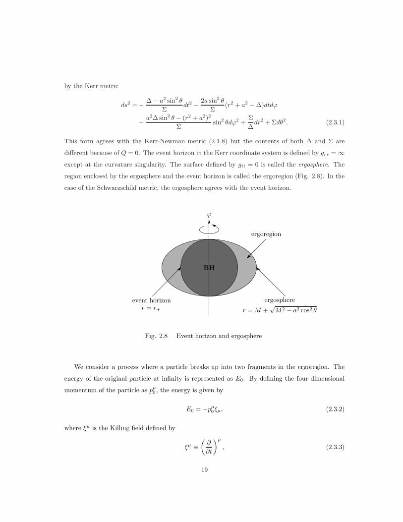
different because of Q = 0. The event horizon in the Kerr coordinate system is defined by grr = ∞except at the curvature singularity. The surface defined by gtt = 0 is called the ergosphere. The
region enclosed by the ergosphere and the event horizon is called the ergoregion (Fig. 2.8). In the
case of the Schwarzschild metric, the ergosphere agrees with the event horizon.
event horizonr = r+
ϕ
ergoregion
r =M +√M2 − a2 cos2 θ
ergosphere
BH
Fig. 2.8 Event horizon and ergosphere
We consider a process where a particle breaks up into two fragments in the ergoregion. The
energy of the original particle at infinity is represented as E0. By defining the four dimensional
momentum of the particle as pµ0 , the energy is given by
E0 = −pµ0 ξµ, (2.3.2)
where ξµ is the Killing field defined by
ξµ ≡(
∂
∂t
)µ
, (2.3.3)
19

which becomes a time translation asymptotically at infinity and is space-like in the ergoregion.
When the particle enters the ergoregion, we arrange to have it break up into two fragments (Fig.
2.9). By the local momentum conservation law, we have
pµ0 = pµ1 + pµ2 , (2.3.4)
where pµ1 and pµ2 are the four dimensional momenta of the two fragments. By contracting the
equation (2.3.4) with ξµ, we obtain the local energy conservation law
E0 = E1 + E2. (2.3.5)
The energy need not be positive in the ergoregion since ξµ is space-like there. We can arrange the
breakup so that one of the fragments has negative total energy,
E1 < 0. (2.3.6)
The fragment with the negative energy falls into the black hole through the event horizon, while
the other can escape to infinity since it does not pass through the event horizon. Therefore, we
can obtain
E2 > E0. (2.3.7)
This means that energy can be classically extracted from a black hole. The above process is called
the Penrose process.
BH E1
E0
E2
Fig. 2.9 Energy extraction from black hole.
20
Of course, all energy cannot be extracted from the black hole by the Penrose process. The
negative energy particle also carry a negative angular momentum, i.e., the angular momentum
opposite to that of the black hole. As a result, the black hole gradually decreases its angular
momentum. When the black hole loses the total angular momentum, it becomes a Schwarzschild
black hole. Since the ergosphere no longer exist in the case of a Schwarzschild black hole, no further
energy extraction can occur.
To see the limit on energy extraction, we use the Killing field χµ defined by
χµ ≡ ξµ +ΩHψµ, (2.3.8)
where ΩH is the angular velocity defined by (2.1.24) and ψµ is the axial Killing field defined by
ψµ ≡(
∂
∂ϕ
)µ
. (2.3.9)
The Killing field is tangent to the null geodesic generators of the horizon and is future directed
null on the horizon. Since the Killing field (2.3.8) is future directed null on the horizon and pµ is
future-directed timelike or null, we have
−pµχµ ≥ 0. (2.3.10)
By substituting (2.3.8) into (2.3.10), we obtain
−pµ(ξµ +ΩHψµ) = ω −mΩH ≥ 0, (2.3.11)
where ω is the energy of the fragment which enters the black hole and m = pµψµ is an angular
momentum of it. In a Kerr black hole background, the system is stationary and has the axial
symmetry. We therefore find that both the energy and the angular momentum are conserved and
these quantities are identified at asymptotic infinity (the Minkowski space). The relation (2.3.11)
is also written as
m ≤ ω
ΩH. (2.3.12)
If ω is negative, m is also negative. Thus the angular momentum of the black hole is reduced. The
mass and the angular momentum of the black hole are respectively M + δM and L + δL where
δM = ω and δL = m. Thus we obtain
δL ≤ δM
ΩH=
2M(
M2 +√M4 − L2
)
LδM, (2.3.13)
21

where we used the formula for ΩH. This is equivalent to
δ
(
1
2
[
M2 +√
M4 − J2]
)
≥ 0. (2.3.14)
Christodoulou defined the irreducible mass Mir by [31]
M2ir ≡
1
2
[
M2 +√
M4 − J2]
(2.3.15)
=1
2
[
M2 +M√
M2 − a2]
. (2.3.16)
The irreducible mass can also be written in terms of the black hole area as in (2.1.20), i.e.,
M2ir =
A
16π. (2.3.17)
By substituting (2.3.17) into (2.3.14), the energy extraction by Penrose process is thus limited by
the requirement that
δA ≥ 0. (2.3.18)
This result agrees with Hawking’s black hole area theorem that the black hole area never decreases
[32].
2.3.2 Superradiance
There is a wave analog of the Penrose process [33, 34]. It is called superradiant scattering or
superradiance. It is known that scalar fields display superradiance. To find this, we consider the
energy current defined by
Jµ ≡ −Tµνξν , (2.3.19)
where Tµν is an energy-momentum tensor which is a symmetric tensor in this case. We take the
covariant derivative ∇µ of (2.3.19)
∇µJµ = −(∇µTµν)ξν − Tµν(∇µξν). (2.3.20)
By the general coordinate invariance, the energy-momentum tensor satisfies
∇µTµν = 0. (2.3.21)
We thus find that the relation (2.3.20) becomes
∇µJµ = −Tµν(∇µξν) (2.3.22)
= −1
2Tµν(∇µξν +∇νξµ) (2.3.23)
= 0, (2.3.24)
22

where we used the facts that the energy-momentum tensor is a symmetric tensor and Killing fields
satisfy the Killing equation
∇µξν +∇νξµ = 0. (2.3.25)
If we integrate (2.3.24) over the region K of space-time whose boundary consists of two spacelike
hypersurfaces Σ1 at t and Σ2 at t+ δt (the constant time slice Σ2 is a time translate of Σ1 by δt)
and two timelike hypersurfaces H (the event horizon at r = r+) and S (∞) (large sphere at spatial
infinity r → ∞), we can know the presence or absence of the superradiance. The intuitive figure
is shown in Fig. 2.10. Strictly speaking, this figure is not precise. The precise figure is shown in
Fig. 2.11 by using Penrose diagram.
nµ
nµ
nµ
nµ
Σ2(t+ δt)
Σ1(t)
δtK
S (∞)H(r+)
Fig. 2.10 Intuitive figure with respect to Gauss’s theorem
I+
I0
H+
nµ
nµ
nµ
Σ2
Σ1
K
Fig. 2.11 Precise figure using the Penrose diagram
23

By using Gauss’s theorem, we obtain
0 =
∫
K
√−gd4x(∇µJµ) (2.3.26)
=
∫
∂K
dΣµJµ (2.3.27)
=
∫
Σ1(t)
nµJµdΣ +
∫
Σ2(t+δt)
nµJµdΣ +
∫
H(r+)
nµJµdΣ +
∫
S (∞)
nµJµdΣ, (2.3.28)
where ∂K is the boundary of the region K, dΣµ ≡ nµdΣ is a 3-dimensional suitable area element
and the unit vector nµ is outwardly normal to the region K. In the last line, the first two terms
cancel with each other because the system has the time translation symmetry and the two directions
of nµ are opposite to each other. The third term represents the flow of the net energy current flux
into the black hole. The last term represents the net energy current flux flow out of K to infinity.
Thus the relation (2.3.28) becomes∫
S (∞)
nµJµdΣ = −
∫
H(r+)
nµJµdΣ. (2.3.29)
If the quantity on the right-hand side in (2.3.29) is positive (negative), this means that the outgoing
energy current flux is larger (smaller) than the incident one and the superradiance is present
(absent).
We would like to evaluate the quantity on the right-hand side in (2.3.29). The vector nµ is
normal to the event horizon. The normal vector nµ can be written in terms of the Killing field χµ
as
nµ = −χµ, (2.3.30)
where χµ is the Killing field defined by (2.3.8). As already stated, one may recall that the Killing
field is tangent to the horizon. One might therefore wonder the appearance of the relation (2.3.30).
This result is known by the fact that the vector which is normal to the horizon is tangent to itself
on the horizon (the null hypersurface). We show a proof in Appendix A. The sign of (2.3.30) is
decided by the direction of nµ toward the horizon which is opposite to the future directed Killing
field. We thus obtain∫
H(r+)
nµJµdΣ = −
∫
H(r+)
χµJµdΣ (2.3.31)
= −∫
H(r+)
χµ (−T µνξ
ν) dΣ (2.3.32)
=
∫
H(r+)
χµTµνξνdΣ, (2.3.33)
24

where we used the definition (2.3.19).
Here we would like to find a concrete form of the energy-momentum tensor Tµν . For sake
of simplicity, we consider the action for a massless scalar field without interactions. In curved
space-time, the action is given by
S ≡∫ √
−gd4x [L] (2.3.34)
=
∫ √−gd4x
[
1
2∇µφ∇µφ
]
, (2.3.35)
where L is the Lagrangian density. According to field theory, the energy-momentum tensor Tµν is
then defined by
Tµν ≡ ∂L∂ (∇µφ)
∇νφ− gµνL (2.3.36)
=1
2(∇µφ)(∇νφ)−
1
2gµν(∇αφ)(∇αφ), (2.3.37)
where we used the Lagrangian density in (2.3.35). By substituting (2.3.37) into (2.3.33), we obtain∫
H(r+)
nµJµdΣ =
∫
H(r+)
dΣ
[
1
2(χµ∇µφ) (ξ
µ∇µφ)−1
2χµξµ (∇αφ) (∇αφ)
]
(2.3.38)
=
∫
H(r+)
dΣ
[
1
2(χµ∇µφ) (ξ
µ∇µφ)
]
, (2.3.39)
where we used the fact that χµξµ = 0 on the horizon. Since we consider the case of a Kerr black
hole which is stationary and axisymmetric, the scalar field can be written asymptotically as
φ(x) = φ0(r, θ) cos(ωt−mϕ). (2.3.40)
Also we asymptotically have
χµ∇µ =∂
∂t+ΩH
∂
∂ϕ, (2.3.41)
ξµ∇µ =∂
∂t. (2.3.42)
We then find that the integrand of (2.3.39) asymptotically becomes
1
2(χµ∇µφ) (ξ
µ∇µφ) =1
2ω(ω −mΩH)φ
2(x) (2.3.43)
where we defined φ(x) ≡ φ0(r, θ) sin(ωt−mϕ). This quantity carried by the Killing field is invariant
on the horizon. The relation (2.3.39) is thus given by∫
H(r+)
nµJµdΣ =
1
2ω(ω −mΩH)
∫
H(r+)
dΣφ2(x). (2.3.44)
25

We note that dΣ = dAdv on the horizon where A is the surface area of the horizon and the retarded
time v is an affine parameter on the horizon. The relation (2.3.44) generally diverges because of
the integration with respect to v. We hence evaluate the energy current flux per unit time. The
time averaged flux becomes∫
S (∞)
nµJµdA = −
∫
H(r+)
nµJµdA (2.3.45)
= −1
2ω(ω −mΩH)
∣
∣
∣φ0
∣
∣
∣
2
. (2.3.46)
where we defined∣
∣
∣φ0
∣
∣
∣
2
≡∫
H(r+)
dAφ2(x). The right-hand side of (2.3.46) is positive for ω in the
range
0 < ω < mΩH. (2.3.47)
Therefore we find that the outgoing energy current flux is larger than the incident one and the
superradiance is present for the scalar field. The above discussion can be similarly performed for
fermion fields. However, it is known that the right-hand side of (2.3.29) alway becomes zero and
the superradiance is hence absent in the fermionic case [35, 36].
2.4 Dimensional Reduction near the Horizon
As stated in Section 2.1, the black hole uniqueness theorem is valid only in four dimensions and
the Kerr-Newman solution is the most general solution in the 4-dimensional theory. The space-time
outside the Kerr-Newman black hole is represented by the Kerr-Newman metric and its geometry
becomes spherically asymmetric because of its own rotation. It is known that the 4-dimensional
Kerr-Newman metric effectively becomes a 2-dimensional spherically symmetric metric by using
the technique of the dimensional reduction near the horizon.
The essential idea is as follows: We consider the action for a scalar field. We can then ignore the
mass, potential and interaction terms in the action because the kinetic term dominates in the high-
energy theory near the horizon. By expanding the scalar field in terms of the spherical harmonics
and using the above properties at horizon, we find that the integrand in the action dose not depend
on angular variables. Thus we find that the 4-dimensional action with the Kerr-Newman metric
effectively becomes a 2-dimensional action with a spherically symmetric metric.
In this section, we would like to discuss the dimensional reduction near the event horizon and
actually show that the 4-dimensional Kerr-Newman metric effectively becomes a 2-dimensional
spherically symmetric metric by using the technique of the dimensional reduction near the horizon.
26

For simplicity, we consider the 4-dimensional action for a complex scalar field
S =
∫
d4x√−ggµν(∂µ + ieVµ)φ
∗(∂ν − ieVν)φ+ Sint, (2.4.1)
where the first term is the kinetic term and the second term Sint represents the mass, potential
and interaction terms. The gauge field Vµ associated with the Coulomb potential of the black hole,
is given by
(Vµ) =
(
− Qr
r2 + a2, 0, 0, 0
)
. (2.4.2)
By substituting both the Kerr-Newman metric (2.1.8) and (2.4.2) to (2.4.1), we obtain
S =
∫
dtdrdθdϕ sin θφ∗
[
(
(r2 + a2)2
∆− a2 sin2 θ
)(
∂t +ieQr
r2 + a2
)2
+ 2ia
(
r2 + a2
∆− 1
)(
∂t +ieQr
r2 + a2
)
Lz − ∂r∆∂r + L2 − a2
∆L2z
]
φ+ Sint, (2.4.3)
where we used
L2 = − 1
sin θ∂θ sin θ∂θ −
1
sin2 θ∂2ϕ, (2.4.4)
Lz = −i∂ϕ. (2.4.5)
By performing the partial wave decomposition of φ in terms of the spherical harmonics
φ =∑
l,m
φlm(t, r)Ylm(θ, ϕ), (2.4.6)
we obtain
S =
∫
dtdrdθdϕ sin θ∑
l′,m′
φ∗l′m′Y ∗l′m′
[
(r2 + a2)2
∆
(
∂t +ieQr
r2 + a2
)2
− a2 sin2 θ
(
∂t +ieQr
r2 + a2
)2
+ 2imar2 + a2
∆
(
∂t +ieQr
r2 + a2
)
− 2ima
(
∂t +ieQr
r2 + a2
)
− ∂r∆∂r + l(l+ 1)− m2a2
∆
]
×∑
l,m
φlmYlm + Sint, (2.4.7)
where we used eigenvalue equations for L2 and Lz
L2Ylm = l(l+ 1)Ylm, (2.4.8)
LzYlm = mYlm. (2.4.9)
27

Here l is the azimuthal quantum number and m is the magnetic quantum number. Now, we
transform the radial coordinate r into the tortoise coordinate r∗ defined by
dr∗dr
=r2 + a2
∆≡ 1
f(r). (2.4.10)
After this transformation, the action (2.4.7) is written by
S =
∫
dtdr∗dθdϕ sin θ∑
l′,m′
φ∗l′m′Y ∗l′m′
[
(r2 + a2)
(
∂t +ieQr
r2 + a2
)2
− f(r)a2 sin2 θ
(
∂t +ieQr
r2 + a2
)2
+ 2ima
(
∂t +ieQr
r2 + a2
)
− F (r)2ima
(
∂t +ieQr
r2 + a2
)
− ∂r∗(r2 + a2)∂r∗
+ f(r)l(l + 1)− m2a2
r2 + a2
]
∑
l,m
φlmYlm + Sint. (2.4.11)
Here we consider this action in the region near the horizon. Since f(r+) = 0 at r → r+, we
only retain dominant terms in (2.4.11). We thus obtain the effective action near the horizon S(H)
S(H) =
∫
dtdr∗dθdϕ sin θ∑
l′,m′
φ∗l′m′Y ∗l′m′
[
(r2 + a2)
(
∂t +ieQr
r2 + a2
)2
+ 2ima
(
∂t +ieQr
r2 + a2
)
− ∂r∗(r2 + a2)∂r∗ −
m2a2
r2 + a2
]
∑
l,m
φlmYlm, (2.4.12)
where we ignored Sint by using f(r+) = 0 at r → r+. Because the theory becomes the high-energy
theory near the horizon and the kinetic term dominates, we can ignore all the terms in Sint. For
example, we consider the case of a mass term. In this case, a mass term is usually given by∫
dx4(
µ2φ∗φ)
=
∫
dtdrdθdϕ sin θ(
µ2φ∗φ)
(2.4.13)
=
∫
dtdr∗dθdϕ sin θ(
f(r)µ2φ∗φ)
, (2.4.14)
where µ is a mass of the scalar field and we used (2.4.10) in the last line. We find that the term
vanishes by using f(r+) = 0 at r → r+. The same is equally true of other interaction terms Sint.
After this analysis, we return to the expression written in terms of r, and we obtain
S(H) = −∑
l,m
∫
dtdr(r2 + a2)φ∗lm
[
− r2 + a2
∆
(
∂t +ieQr
r2 + a2+
ima
r2 + a2
)2
+ ∂r∆
r2 + a2∂r
]
φlm,
(2.4.15)
where we used the orthonormal condition for the spherical harmonics∫
dθdϕ sin θY ∗l′m′Ylm = δl′,lδm′,m. (2.4.16)
28

From (2.4.15), we find that φlm can be considered as a (1+1)-dimensional complex scalar field
in the backgrounds of the dilaton Φ, metric gµν and two U(1) gauge fields Vµ, Uµ
Φ = r2 + a2, (2.4.17)
gtt = −f(r), grr =1
f(r), grt = 0, (2.4.18)
Vt = − Qr
r2 + a2, Vr = 0, (2.4.19)
Ut = − a
r2 + a2, Ur = 0. (2.4.20)
There are two U(1) gauge fields: One is the original gauge field as in (2.4.2) while the other is the
induced gauge field associated with the isometry along the ϕ direction. The induced U(1) charge
of the 2-dimensional field φlm is given by m. Then the gauge potential At is a sum of these two
fields,
At ≡ eVt +mUt = − eQr
r2 + a2− ma
r2 + a2, Ar = 0. (2.4.21)
By using the above notations, the action (2.4.15) is rewritten as
S(H) = −∑
l,m
∫
dtdrΦφ∗lm
[
gtt (∂t − iAt)2 + ∂rg
rr∂r
]
φlm, (2.4.22)
From (2.4.18), we find that the 4-dimensional spherically non-symmetric Kerr-Newman metric
(2.1.8) effectively behaves as a 2-dimensional spherically symmetric metric in the region near the
horizon only
ds2 = −f(r)dt2 + 1
f(r)dr2. (2.4.23)
For confirmation, we show how to derive the surface gravity on the horizon of the Kerr-Newman
black hole from f(r) defined by (2.4.10). Actually by calculating the surface gravity, we can obtain
κ± ≡ 1
2f ′(r)
∣
∣
∣
∣
∣
r=r±
=r± − r∓
2(r2± + a2), (2.4.24)
where ′ represents differentiation with respect to r. This result agrees with the well-known
surface gravity on the horizon of the Kerr-Newman black hole as in (2.1.23).
2.5 Analogies between Black Hole Physics and Thermody-
namics
To understand properties of black holes, it is very useful to understand the black hole physics
in the context of generalized thermodynamics. The main reason is that there are various analogies
29

between the black hole physics and thermodynamics. It is said that the idea of making use of
thermodynamic methods in black hole physics appears to have been first considered by Greif. He
examined the possibility of defining the entropy of a black hole, but lacking many of the recent
results in black hole physics, he did not make a concrete proposal [37]. Afterward, properties of
black holes were analyzed by Bekenstein, Bardeen, Carter and Hawking and others, and analogies
between black hole physics and thermodynamics were clarified [38,39]. The discussion is as follows.
By definition, a black hole can absorb matter but nothing, not even light, can classically escape
from it. A black hole has a property that as a black hole absorbs matter, the black hole area
increases. For example, we consider that two Schwarzschild black holes with masses M1 and M2
merge and then a black hole with a mass M =M1 +M2 is formed (Fig. 2.12). Before the merger,
areas of two black holes are respectively A1 = 16πM21 and A2 = 16πM2
2 . An area of the black
hole after the merger is A = 16π(M1 +M2)2. Compared between the sum of two black hole areas
before the merger and the black hole area after the merger, we obtain an inequality for black hole
areas
A1 +A2 ≤ A. (2.5.1)
This means that a black hole area after the merger is the same as the sum of each black hole area
before the merger or is larger than it. A black hole area never classically decreases,
δA ≥ 0, (2.5.2)
since no black hole radiates matter or splits into any black holes. This result is known as Hawking’s
black hole area theorem [32].
30

+
A1 = 16πM21 A2 = 16πM2
2 A = 16π(M1 +M2)2
M1 M2 M
Fig. 2.12 The merger of black holes.
Here we would like to state the properties of entropy in thermodynamics. In thermodynamics,
entropy represents the degree of concentration of matter and energy in a system. As a famous
example of explaining entropy, we consider that one puts a drop of ink into a glass of water. At
first, a drop of ink localizes in a certain part of the water. This is a state with low entropy. As
time advances, a drop of ink distributes all over the water and the water achieve an even color at
some time. This is that entropy is a state with higher entropy. The entropy of an isolated system
S never decreases and rather increases over time, i.e.,
δS ≥ 0. (2.5.3)
This is well-known as the second law of thermodynamics. Thus, both of the black hole area and
entropy tend to increase irreversibly.
As with entropy, the black hole area is closely related to a degradation of energy, in other words,
an unavailable energy. In thermodynamics, an increase of entropy means that a part of energy
is unavailable, namely, the energy is no longer converted into work. There is the same relation
in black hole physics. In Section 2.3, we showed that a part of energy can be extracted from a
rotating black hole such as a Kerr black hole by the Penrose process. But all energy cannot be
extracted from the black hole. The Kerr black hole gradually decreases the angular momentum
by the Penrose process. When the black hole loses the total angular momentum, it becomes a
Schwarzschild black hole. By the Hawking’s black hole area theorem, the mass of the black hole
is then larger than a mass of a Schwarzschild black hole obtained by taking a = 0 for the original
Kerr black hole. This mass is called an irreducible mass. In the case of a Kerr-Newman black hole,
the irreducible mass Mir is given by
Mir =
√
A
16π. (2.5.4)
31

It is regarded as an inactive energy which cannot be converted to work. The increase of an
irreducible mass Mir, i.e., the increase of a black hole area A thus corresponds to a degradation of
the black hole energy in the thermodynamic sense.
As found from the above consideration, it is said that properties possessed by a black hole area
A are similar to ones possessed by the thermodynamic entropy and the Hawking’s black hole area
theorem corresponds to the second law of thermodynamics. Furthermore, by comparing the energy
conservation law in the black hole physics with the first law of thermodynamics, we would like to
clarify corresponding physical quantities in these two phenomena.
In general, the first law of thermodynamics is given by
dE = T dS − dW , (2.5.5)
where E is the energy of the system, T is the temperature, S is the entropy and W is the work
done by the system, while as already stated as in (2.1.22) of Section 2.1, the energy conservation
law in black hole physics is given by
dM =κ
8πdA+ΩHdL+ΦHdQ, (2.5.6)
Now we make comparisons between the relations (2.5.5) and (2.5.6). We make a table of the
corresponding relationships between physical quantities of black hole physics and thermodynamics
(Tab. 2.3). The correspondence relationship between the mass M and the energy E in the left
side of each relation is clear and it is well-known as the mass-energy equivalence by Einstein.
The second term and the third term in (2.5.6) stand for work terms done by the rotation and
the electromagnetism. It is considered that they correspond to the work term −dW done by the
system in thermodynamics. We shall compare the remaining first term in each relation, i.e.,κ
8πdA
and T dS. By making a black hole area correspond to entropy, we find that the surface gravity
corresponds to the temperature in thermodynamics.
32

Tab. 2.3 The corresponding relationships between physical
quantities of thermodynamics and black hole physics
Thermodynamics Black hole physics
Energy: E Mass: M
Temperature: T Surface gravity: κ
Entropy: S Black hole area: A
Work term done by system: Work terms done by rotation and−dW electromagnetism: ΩHdL+ΦHdQ
Here we recall properties of both the surface gravity of a black hole and temperature. By
definition, a surface gravity of the black hole represents the strength of the gravitational field on
the event horizon. As found from (2.1.23), the surface gravity κ is constant over the horizon in the
stationary black hole. In thermal equilibrium, temperature also possesses the same property. It is
well-known as the zeroth law of thermodynamics.
In passing, the third law of thermodynamics states that the temperature of the system cannot
achieve the absolute zero temperature by a physical process. This is also called Nernst’s theorem.
It corresponds to the speculation that the surface gravity cannot achieve κ = 0 by a physical
process in black hole physics. A reason for believing it is that if one could reduce it to zero by a
finite sequence of operations, then presumably one could carry the process further, thereby creating
a naked singularity.
From the above discussion, we find that the relationships between the laws of black hole physics
and thermodynamics may be more than an analogy (Tab. 2.4, [40]). However, we do not know
from only the above discussion that black holes actually have entropy and temperature. In the
next section, we would like to discuss the consideration that black holes have entropy, which is due
to Bekenstein.
33

Tab. 2.4 The corresponding relationships between the laws
of thermodynamics and black hole physics
Law Thermodynamics Black hole physics
Zeroth T constant throughout body κ constant over horizonin thermal equilibrium of stationary black hole
First dE = T dS − dW dM =κ
8πdA+ΩHdL +ΦHdQ
Second δS ≥ 0 in any process δA ≥ 0 in any process
Third Impossible to achieve T = 0 Impossible to achieve κ = 0by a physical process by a physical process
2.6 Black Holes and Entropy
In 1973, Bekenstein proposed that a black hole has its entropy. He stated that the black hole
entropy is represented by a function of the black hole area from the above analogies. If the black
hole entropy is related to the black hole area, it has to satisfy the black hole area theorem. From
this, he presumed that the black hole entropy is proportional to the black hole area.
Then, to find the proportionality coefficient, he considered that a particle with the least infor-
mation falls into a black hole. When the particle falls into a black hole, the information of the
particle is lost. In other words, it means an increase in the black hole entropy. He evaluated the
proportionality coefficient by the conjecture that the black hole entropy equals the minimum area
increased by dropping a matter into the black hole.
In this section, we would like to show the derivation of black hole entropy by Bekenstein.
In Subsection 2.6.1, we simply explain the entropy of a particle with the least information in
information theory. In Subsection 2.6.2, we explain that minimum entropy is increased when a
particle falls into a black hole. In Subsection 2.6.3, we evaluate the black hole entropy by using
assumptions that these two quantities are equal to each other.
34
2.6.1 Entropy in information theory
In physics, entropy represents a degree of concentration of matter and energies. The entropy
is defined by Boltzmann’s formula
S = k lnW, (2.6.1)
where W is the number of states and k is Boltzmann’s constant.
The connection between entropy and information is well-known [41,42]. In information theory,
the uncertain information and the missing information of the system are measured by the entropy.
The probability of the n-th state in all known states of the system is defined as Pn The entropy of
the system is then defined by Shannon’s formula
S = −∑
n
Pn lnPn. (2.6.2)
Here we note that entropy is dimensionless. We will present the discussion of dimensions later.
When a new piece of information is available for the system, we can find that probabilities Pn
are provided with some restrictions. For example, we consider the case of a die. The probabilities
are respectively 16 from 1 to 6. The entropy is then ln 6 from (2.6.2). Now if we get new information
that “There are odd numbers (or odd numbers are given)”, then the probability of getting even
numbers is zero, i.e., P2 = P4 = P6 = 0. The probability of getting odd numbers is 13 and thus the
entropy is ln 3. As found in the above discussion, as we get new information, the entropy locally
decreases. This property is given by Brillouin’s identification [43]
∆I = −∆S, (2.6.3)
where ∆I stands for the new information (bound information). This relation means that the
bound information corresponds to the decrease of the entropy.
Here we would like to discuss the dimensions of the physical quantities. Entropy appearing in
Boltzmann’s formula (2.6.1) has the dimension of the energy divided by the temperature. Although
it is possible to decide the dimension of information by using it, it is a custom in the information
theory to treat information as a dimensionless quantity. Thus we adopt a unit system that both
entropy and information is dimensionless. This means we select to measure temperature by the
unit of energy. Then Boltzmann’s constant is also dimensionless. By adopting the above unit
system, the equations (2.6.2) and (2.6.3) are satisfied as dimensionless quantities.
35

The conventional unit of information is the “bit” which may be defined as the information
available when the answer to a yes-or-no question is precisely known, i.e., the entropy is zero.
Of course, the unit is dimensionless. According to (2.6.3), a bit is also numerically equal to the
maximum entropy that can be associated with a yes-or-no question, i.e., the entropy when no
information whatsoever is available about the answer. From (2.6.2), the entropy in the yes-or-no
question is written as
S = −Pyes lnPyes − Pno lnPno (2.6.4)
= −Pyes lnPyes − (1− Pyes) ln(1− Pyes). (2.6.5)
We thus find that the entropy is the maximum value ln 2 when Pyes = Pno =1
2and one bit is equal
to ln 2 of information.
Let us now return to our original subject, black hole. We consider that a particle falls into
a black hole. An amount of information of the particle would depend on how much is known
about the internal states of the particle. The minimum information loss for the particle would
be contained in the answer to the question “Does the particle exist or not?” Before the particle
drops into the black hole, the answer is known to be “yes”. But after the particle drops into the
black hole, we have no information whatever about the answer. This is because one knows nothing
about the physical conditions inside the black hole, and thus one cannot assess the likelihood of
the particle continuing to exist or being destroyed. One must, therefore, admit the loss of one bit
of information at the very least. This means that the entropy is increased by
∆S = ln 2, (2.6.6)
before and after the particle with the tiniest information falls into the black hole.
2.6.2 The minimum increase of the black hole area
In this subsection, we calculate the minimum possible increase in the black hole area, which
must result when a spherical particle of rest mass µ and proper radius b is captured by a Kerr-
Newman black hole. Bekenstein used the “rationalized area” of a black hole α defined by
α ≡ A
4π, (2.6.7)
where A is the black hole area as in (2.1.20). The first law of black hole physics (2.1.22) is then
written as
dM = ΘHdα+ΩHdL+ΦHdQ, (2.6.8)
36

where ΘH is defined by
ΘH ≡ r+ −M
2α. (2.6.9)
There are several ways in which a particle may fall into a black hole. All these bring the increase
of the black hole area. We are interested in the method for inserting the particle which results
in the smallest increase. This method has already been discussed by Christodoulou in connection
with his introduction of the concept of irreducible mass [31, 44]. The essence of Christodoulou’s
method is that if a freely falling point particle is captured by a Kerr-Newman black hole, then
the irreducible mass and, consequently, the area of the black hole is left unchanged. Bekenstein
generalized Christodoulou’s method to a particle with a proper radius and showed the increased
area of the black hole is no longer precisely zero when the particle falls into the black hole.
We assume that a freely falling particle is neutral. The trajectory of the particle follows a
geodesic of the Kerr-Newman metric (2.1.8). The horizon is located at r = r+ where r± are
defined by (2.1.17).
First integrals for geodesic motion in the Kerr-Newman background have been given by Carter
[45]. Christodoulou used the first integral
E2[r4+a2(r2+2Mr−Q2)]−2E(2Mr−Q2)apϕ−(r2−2Mr+Q2)p2ϕ−(µ2r2+q)∆ = (pr∆)2, (2.6.10)
as a starting point of his analysis. We show the derivation in Appendix B. In (2.6.10), E = −ptis the conserved energy, pϕ is the conserved component of angular momentum in the direction of
the axis of symmetry, q is Carter’s fourth constant of the motion, µ is the rest mass of the particle
and pr is its covariant radial momentum.
By following Christodoulou, we solve (2.6.10) for E:
E = Bapϕ +
√
(
B2a2 +r2 − 2Mr +Q2
A
)
p2ϕ +(µ2r2 + q)∆ + (pr∆)2
A , (2.6.11)
where
A ≡ r4 + a2(r2 + 2Mr −Q2), (2.6.12)
B ≡ (2Mr −Q2)
A . (2.6.13)
The definitions (2.6.12) and (2.6.13) at the horizon as in (2.1.16) are written as
A(r = r+) ≡ A+ = (r2+ + a2)2, (2.6.14)
B(r = r+) ≡ B+ =1
r2+ + a2. (2.6.15)
37

Furthermore, at the horizon, we obtain
B+a = ΩH. (2.6.16)
where ΩH is defined by (2.1.24). The coefficient of p2ϕ at the horizon vanishes
B2+a
2 +r2+ − 2Mr+ +Q2
A+=
a2
(r2+ + a2)2+r2+ − 2Mr+ +Q2
(r2+ + a2)2=
∆
(r2+ + a2)2= 0, (2.6.17)
and the coefficient of µ2r2 + q also vanishes. However, since pr∆ cannot be defined at the horizon
because of pr = grrpr, we retain the term as
pr =Σ
∆pr (2.6.18)
⇔ pr∆ = (r2 + a2 cos2 θ)pr. (2.6.19)
If the particle’s orbit intersects the horizon, we then have from (2.6.11) that
E = ΩHpϕ +|pr∆|+√
A+
. (2.6.20)
As a result of the capture, the mass of the black hole increases by E and its component of the
angular momentum in the direction of the symmetry axis increases by pϕ. By comparing (2.1.22)
with (2.6.20), the black hole’s rationalized area α increases by|pr∆|+ΘH
√
A+
. As pointed out by
Christodoulou, by taking
|pr∆|+ = 0, (2.6.21)
the relation (2.6.20) becomes
E = ΩHpϕ, (2.6.22)
and the increase of the black hole area vanishes. The above analysis shows that it is possible for a
black hole to capture a point particle without increasing its area.
Here, by following Bekenstein’s extension, we would like to show how this conclusion is changed
if the particle has a nonzero proper radius b. The relation (2.6.11) always describes the motion
of the particle’s center of mass at the moment of capture. It should be clear that to generalize
Christodoulou’s result to the present case one should evaluate (2.6.11) not at r = r+, but r = r++δ,
where δ is determined by
∫ r++δ
r+
√grrdr = b. (2.6.23)
38

r = r+ + δ is a point a proper distance b outside the horizon. By using the component grr as in
(2.1.15), we find
b = 2
√
δ(r2+ + a2 cos2 θ)
r+ − r−, (2.6.24)
where we assumed that r+ − r− ≫ δ. Expanding the argument of the square root in (2.6.11) in
powers of δ, replacing δ by its value given by (2.6.24), and keeping only terms to O(b) we obtain
E = ΩHpϕ +
√
(
r2+ − a2
r2+ + a2
)
p2ϕ + µ2r2+ + q × 1
2br+ − r−(r2+ + a2)
× 1√
r2+ + a2 cos2 θ. (2.6.25)
This relation (2.6.25) is the generalization to O(b) of Christodoulou’s result (2.6.22). Carter’s
kinetic constant q is given by
q = cos2 θ
[
a2(µ2 − E2) +p2ϕ
sin2 θ
]
+ p2θ (2.6.26)
This constant appeared in the derivation of (2.6.10) (see Appendix B). We can obtain a lower
bound for it as follows. From the requirement that the θ momentum pθ is real in (2.6.26), we
obtain
q ≥ cos2 θ
[
a2(µ2 − E2) +p2ϕ
sin2 θ
]
, (2.6.27)
where the equality holds when pθ = 0. If we replace E in (2.6.27) by ΩHpϕ as in (2.6.22), we obtain
q ≥ cos2 θ
[
a2µ2 + p2ϕ
(
1
sin2 θ− a2Ω2
H
)]
. (2.6.28)
We know that1
sin2 θ≥ 1 and it is easily shown that a2Ω2
H ≤ 1
4for a Kerr-Newman black hole.
Since the coefficient of p2ϕ is positive, we can take the constant q as a smaller value
q ≥ a2µ2 cos2 θ, (2.6.29)
when pϕ = 0. By substituting (2.6.29) into (2.6.25), we obtain
E ≥ ΩHpϕ +1
2µbr+ − r−r2+ + a2
, (2.6.30)
where the equality holds when pϕ = pθ = pr = 0. This relation is correct to O(b). The increase in
the rationalized area of the black hole, computed by means of (2.6.8), (2.6.9) and (2.6.30), is given
by
∆α ≥ 2µb. (2.6.31)
39

This gives the fundamental lower bound on the increase in the rationalized area of the black hole
∆α,
(∆α)min = 2µb. (2.6.32)
We note that it is independent of M , Q and L.
We can make (∆α)min smaller by making b smaller. However, we must remember that b can
be no smaller than the particle’s Compton wavelength~
µ, or the Schwarzschild radius 2µ. If the
Compton wavelength is larger than the Schwarzschild radius~
µ≥ 2µ, namely, the mass of the
particle satisfies µ ≤√
~
2, we can make b smaller to
~
µ. If the Schwarzschild radius is larger than
the Compton wavelength~
µ< 2µ, namely, the mass of the particle satisfies µ >
√
~
2, we can make
b smaller to 2µ. The relation (2.6.32) is thus given by 2~, when b =~
µ, and given by 4µ2, when
b ≃ 2µ. Since 4µ2 > 2~, we can determine a lower bound of the rationalized area of a Kerr-Newman
black hole as
(∆α)min = 2~, (2.6.33)
when the black hole captures the particle.
2.6.3 Information loss and black hole entropy
In Section 2.5, we already stated that a black hole area is similar to the entropy in thermo-
dynamics. Although there are clear analogies between them, we do not know how to identify the
black hole area as the black hole entropy. In this subsection, we would like to present the discussion
by Bekenstein [38].
To begin with, we consider that a black hole is formed by the gravitational collapse of a
very heavy star. According to the no-hair theorem [16], the stationary state of the black hole
is completely characterized by three parameters, i.e., the mass, the angular momentum and the
charge. Thus black holes do not depend on the internal configuration of the collapsed body. This
means that a lot of information is lost by the gravitational collapse. It is then natural to introduce
the concept of black hole entropy as the measure of the inaccessibility of information to an exterior
observer. Furthermore, we consider that the black hole entropy is associated with the black hole
area.
40

Bekenstein assumed that the entropy of a black hole SBH is some monotonically increasing
function of its rationalized area as in (2.6.7):
SBH = f(α). (2.6.34)
The entropy of an evolving thermodynamic system increases due to the gradual loss of information
which is a consequence of the washing out of the most of the initial conditions. Now, as a black
hole approaches equilibrium, the effects of the initial conditions are also washed out (the black hole
loses its hair). One would thus expect that the loss of information about initial peculiarities of the
black hole will be reflected in a gradual increase in SBH. Indeed the relation (2.6.34) predicts just
this.
One possible choice for f in (2.6.34),
f(α) ∝√α, (2.6.35)
is untenable on some reasons. We consider two black holes which start off very distant from each
other. Since they interact weakly, we can take the total black hole entropy to be the sum of
SBH of each black hole. The black holes now move closer together and finally merge, and form
a black hole which settles down to equilibrium. In the process no information about the black
hole interior can become available. On the contrary, much information is lost as the final black
hole loses its hair. Thus, we expect the final black hole entropy to exceed the initial one. By the
assumption (2.6.35), this implies that the irreducible mass (2.5.4) of the final black hole exceeds
the sum of irreducible masses of the initial black holes. Now suppose that all three black holes
are Schwarzschild (M = Mir). We are then confronted with the prediction that the final black
hole mass exceeds the initial one. But this is nonsensical since the total black hole mass can
only decrease due to gravitational radiation losses. We thus see that the choice as in (2.6.35) is
untenable.
The next simplest choice for f is
f(α) = γα, (2.6.36)
where γ is a constant. Repetition of the above argument for this new f leads to the conclusion
that the final black-hole area must exceed the total initial black hole area. But we know this to be
true from Hawking’s theorem [32]. Thus the choice (2.6.36) leads to no contradiction. Therefore,
Bekenstein adopted (2.6.36) for the moment.
41

Comparison of (2.6.35) and (2.6.36) shows that γ must have the units of [length]−2. But there
is no constant with such units in classical general relativity. And so Bekenstein found only one
truly universal constant ~−1 with the correct units, where ~ is the Planck constant. Until now,
although we used the natural system of units (1.0.1), we shall clearly describe the constant ~ in
this subsection. Thus Bekenstein represented (2.6.34) as
SBH =ηα
~, (2.6.37)
where η is a dimensionless constant. This expression was also proposed by Bekenstein earlier from
a different point of view [46]. It is well known that the Planck constant ~ also appears in the
formulas for the entropy in thermodynamics, for example, the Sackur-Tetrode equation (see, for
example, [47]).
To determine the value of η, Bekenstein considered that a particle falls into a Kerr-Newman
black hole. In Subsection 2.6.1, we showed that the loss of one bit of information before and
after the particle with the least information falls into a black hole, i.e., the increased entropy is
∆S = ln 2. In Subsection 2.6.2, we showed that when a spherical particle with a radius, which is
as large as the Compton wavelength, falls into a black hole, the minimum increase of the black
hole area is given by (2.6.32). From (2.6.32), we obtain the increase of black hole entropy given by
(∆SBH)min = 2~df(α)
dα. (2.6.38)
Bekenstein conjectured that this entropy agrees with the loss of one bit of information (2.6.6) (see
Fig. 2.13). We thus obtain
2~df(α)
dα= ln 2. (2.6.39)
In the left-hand side of (2.6.39), the limit as in (2.6.33) can be attained only for a particle whose di-
mension is given by its Compton wavelength. Only such an “elementary particle” may be regarded
as having no internal structure. We can thus consider that the loss of information associated with
the loss of such a particle should be minimum. By integrating (2.6.39) over α, we obtain
f(α) =
(
1
2ln 2
)
α
~. (2.6.40)
From (2.6.34), we can obtain the black hole entropy
SBH =
(
1
2ln 2
)
α
~. (2.6.41)
This form agrees with that of (2.6.37).
42

ln 2
BH BH
SBH
Fig. 2.13 Information loss and increase of entropy
Bekenstein showed the dependence of the black hole entropy SBH on the black hole area α from
the above discussion, and the black hole entropy is given by
SBH =ln 2
8π
kc3
~GA, (2.6.42)
where we write the conventional units explicitly. However, he used some conjectures, and the
relation η = 12 ln 2 is derived by a certain assumption. The assumption is that the smallest possible
radius of a particle is precisely equal to its Compton wavelength whereas the actual radius is not
so sharply defined. Furthermore, an amount of information of such a particle might be more than
ln 2 because the particle has information for the mass and the radius. According to the current
understanding, the black hole entropy is given by
SBH =1
4
kc3
~GA. (2.6.43)
In comparison between (2.6.42) and (2.6.43), the value of η is slightly different. However, Beken-
stein had stated in his paper [38] that it would be somewhat pretentious to attempt to calculate
the precise value of the constantη
~without a full understanding of the quantum reality which
underlies a “classical” black hole. Surprisingly, he already suggested that the derivation of black
hole radiation needs the consideration of quantum theory.
Bekenstein also defined a characteristic temperature for a Kerr-Newman black hole by
1
TBH=
(
∂SBH
∂M
)
L,Q
, (2.6.44)
which is an analogue of the thermodynamic relation
1
T =
(
∂S∂E
)
V
. (2.6.45)
43

By using both (2.6.8) and (2.6.9) in (2.6.44), we can obtain
T =2~
ln 2ΘH. (2.6.46)
But Bekenstein did not regard this temperature as the temperature of the black hole. Because if
a black hole has a temperature, some radiation from the black hole may appear. This conflicts
with the classical definition. By definition, a black hole can only absorb matter but cannot radiate
matter. Bekenstein did not suggest that a black hole has a temperature for the above reason.
44
Chapter 3
Black Hole Radiation
In the classical theory, black holes can only absorb matter but cannot radiate matter. Beken-
stein proposed that a black hole has entropy from the point of view of information theory but
could not suggest that a black hole has a temperature from his reasoning. Therefore, the complete
correspondence between black hole physics and thermodynamics cannot be obtained. However,
Hawking showed that a black hole continuously radiates its energy by taking quantum effects into
account [2]. Furthermore, it was found that a black hole behaves as the a black body with a
certain temperature and continuously performs its radiation. This is consistent with the classical
definition of black holes. This black hole radiation is commonly called Hawking radiation.
The intuitive explanation is as follows [48]: According to quantum field theory, it is considered
that a particle-antiparticle pair is formed by a fluctuation of energy everywhere in our universe.
The antiparticle (negative energy state) formed by the pair creation can exist only for a very short
time since it is unstable in our universe. The particle-antiparticle pair therefore vanishes by the
pair annihilation after a certain short period of time.
Now we consider a pair creation very close to the event horizon outside a black hole. The pair
creation arises in globally curved space-time because general relativity is based on the assumption
that the space-time can be made locally flat. If a particle-antiparticle pair is formed very close to
the horizon, the antiparticle (negative energy state) can fall into the black hole through the horizon
in a certain short period of time. It is possible to show that the antiparticle can be put into a
realizable orbit inside the event horizon. For an external observer, the black hole decreases its
energy by absorbing the negative energy (antiparticle), while the particle with the positive energy,
which is the same amount as the decreased energy of the black hole, can escape to infinity, since it
can stably exist in our universe (Fig. 3.1). Therefore, we can understand that black holes radiate
45

particles. This is the mechanism of Hawking radiation.
BH−E
EBH
E
Hawking radiation
Fig. 3.1 Hawking mechanism
In this chapter, we would like to present several previous works on Hawking radiation. For
sake of simplicity, we consider the case of a Schwarzschild black hole. The contents of this chapter
are as follows. In Section 3.1, we review Hawking’s original derivation of Hawking radiation. In
Section 3.2, we would like to discuss some representative derivations of Hawking radiation briefly.
3.1 Hawking’s Original Derivation
Hawking showed that black holes radiate matter by using quantum field theory in black hole
physics. In this section, we would like to show the original derivation of Hawking radiation by
Hawking [2].
For sake of simplicity, we consider a free massless scalar field. In Minkowski space, it satisfies
the Klein-Gordon equation
ηµν∂µ∂νφ = 0, (3.1.1)
where φ is a massless hermitian scalar field, ηµν is the Minkowski metric (2.1.12) and ∂µ is the
partial derivative defined by
∂µ ≡ ∂
∂xµ. (3.1.2)
The ordinary derivative of φ is also written as φ,µ. We can decompose the field into positive and
negative frequency components
φ =∑
i
(ϕiai + ϕ∗ia
†i ), (3.1.3)
46

where ϕi are a complete orthonormal family of complex valued solutions of the wave equation
ηµν∂µ∂νϕ = 0. (3.1.4)
It contains only positive frequencies with respect to the usual Minkowski time coordinate. The
operators ai and a†i are interpreted as the annihilation and creation operators respectively for
particles in the i-th state. The vacuum state |0〉 is defined to be the state from which one cannot
annihilate any particle, i.e.,
ai|0〉 = 0, for all i. (3.1.5)
The orthonormal condition is then given by
ρM (ϕi, ϕj) ≡1
2i
∫
V
(ϕi∂tϕ∗j − ϕ∗
j∂tϕi)dx3 = δij , (3.1.6)
where V is a suitable closed space.
We considered quantum field theory in Minkowski space so far. Here, we would like to extend
Minkowski space-time to curved space-time which is produced by the intense gravity of a black
hole. In the curved space-time, the metric changes from the Minkowski metric to the metric of the
curved space-time. Also physical laws must hold in any coordinate system. The partial derivatives
contained in these laws must be replaced by the covariant derivatives in the curved space-time [49].
The covariant derivative is commonly represented by
∇µ ≡ φ;µ. (3.1.7)
The covariant derivative for a scalar field φ is given by
∇µφ = ∂µφ, (3.1.8)
and the covariant derivative for a vector field Aν is given by
∇µAν = ∂µAν + ΓανµAα, (3.1.9)
where Γανµ is the Christoffel symbol defined by (2.1.5). In curved space-time, the Klein-Gordon
equation for a massless hermitian scalar field is thus represented by
gµν∇µ∇νφ = 0. (3.1.10)
47

We can use the relation (3.1.3) in the flat space. However, we cannot decompose the field into
positive and negative frequency components in curved space. One can still require that the fiand the f∗
i together form a complete the basis for solutions of the wave equations with
ρ(ϕi, ϕj) = −1
2i
∫
Σ
(ϕi∇µϕ∗j − ϕ∗
j∇µϕi)dΣµ = δij , (3.1.11)
where dΣ stands for an area element and Σ is called a Cauchy surface which represents a suitable
surface.
Here we recall the Penrose diagram drawn in Fig. 2.7. In the past null infinity J−, the
Schwarzschild metric is asymptotically flat (the Minkowski metric) since r → ∞. We can thus
expand the field operator φ which satisfies the Klein-Gordon equation (3.1.10) as
φ =∑
i
fiai + f∗i a
†i, (3.1.12)
where fi is a family of solutions of the wave equation
ηµν∇µ∇νfi = 0. (3.1.13)
In a manner similar to (3.1.11), they satisfy the orthonormal condition at J −
ρ(fi, f∗j ) =
1
2i
∫
Σ
(fi∇µf∗j − f∗
j ∇µfi)dΣµ = δij , (3.1.14)
where we note that fi only contain positive frequencies with respect to the canonical affine
parameter on J−. It is natural that the operators ai and a†i are respectively regarded as the
annihilation and creation operators at J −. The vacuum at J− is thus defined by
ai|0−〉 = 0. (3.1.15)
Similarly, in the future null infinity J +, the Schwarzschild metric is asymptotically flat since
r → ∞. We can also expand the field operator φ by
φ =∑
i
pibi + p∗i b†i + qici + q∗i c
†i
, (3.1.16)
where pi are solutions of the wave equation which can escape to J+ and qi are solutions of the
wave equation which cannot escape to J + since they are absorbed by the future event horizon H+,
namely, pi are zero at H+ and qi are zero at J +. The operators bi and b†i respectively stand
for the annihilation and creation operators at J +, and the operators ci and c†i respectively stand
48

for the annihilation and creation operators at H+. The vacua at J + and H+ are thus defined by
bi|0+〉 = 0, (3.1.17)
ci|0H+〉 = 0, (3.1.18)
where we also note that pi contain positive frequencies only with respect to the canonical affine
parameter on J +. Although it is not clear whether one should impose some positive frequency
condition on qi, we would like to consider particles which start from J −, pass through the
collapsing body and can escape to J+. The choice of the qi does not affect the calculation of
the emission of particle to J + since the qi are zero at J+. We require that pi and p∗i are a
complete orthonormal family which satisfies
ρ′(pi, p∗j ) =
1
2i
∫
Σ′
(pi∇µp∗j − p∗j∇µpi)dΣ
′µ = δij . (3.1.19)
Here we would like to show that the relation (3.1.19) is satisfied even if one uses Σ which
appeared in (3.1.14) instead of Σ′. We thus consider ρ(pi, p∗j )− ρ′(pi, p
∗j ). If the stable surface Σ′
differs from Σ, Σ′ can smoothly intersect with Σ at certain points since Σ′ is not parallel to Σ. We
represent the 4-dimensional volume enclosed by these two surfaces as V (Fig. 3.2). By using the
4-dimensional Gauss theorem, we obtain
ρ(pi, p∗j )− ρ′(pi, p
∗j) =
∫
V
d4x√−g∇µ(pi∇µp
∗j − p∗j∇µpi), (3.1.20)
where g stands for the determinant of the metric gµν defined by
g ≡ det (gµν) , (3.1.21)
namely,√−g stands for the Jacobian with respect to the transformation from d4x to dΣ. By
calculating the integrand of the right-hand side in (3.1.20), we obtain
∇µ(pi∇µp∗j − p∗j∇µpi) =∇µpi∇µp
∗j + pi∇µ∇µp
∗j −∇µp∗j∇µpi − p∗j∇µ∇µpi
=pi∇µ∇µp∗j − p∗j∇µ∇µpi. (3.1.22)
By using the Klein-Gordon equation (3.1.10), the relation (3.1.22) becomes
∇µ(pi∇µp∗j − p∗j∇µpi) = 0. (3.1.23)
Since the right-hand side of (3.1.19) is zero, we obtain
ρ(pi, p∗j) = ρ′(pi, p
∗j ). (3.1.24)
49

This means that ρ(pi, p∗j) does not depend on Σ. Namely, if the Gauss theorem is satisfied, it
means that we can freely choose the surface Σ in (3.1.11)
ρ(pi, p∗j ) =
1
2i
∫
Σ
(pi∇µp∗j − p∗j∇µpi)dΣ
µ = δij . (3.1.25)
It is known that the above discussion is also valid for a scalar field with a mass [50].
Σ′
Σ
V
Fig. 3.2 The volume V enclosed by two surfaces Σ and Σ′
In the transitional time between fi and pi, a collapsing body will appear. We do not know
the corresponding solutions since we do not know the metric inside this region. By using the analogy
of the tunneling effect, we can represent pi which appear at J+ as the linear combinations of
fi with f∗i
pi =∑
j
(αijfj + βijf∗j ), (3.1.26)
where αij and βij are proportionality coefficients which stand for the amplitude ratio (Fig. 3.3).
We substitute (3.1.26) into (3.1.16). Since qi = 0 at J+, the relation (3.1.16) becomes
φ =∑
i
∑
j
(bjαij + b†jβ
∗ij)fi +
∑
j
(bjβij + b†jα
∗ij)f
∗i
. (3.1.27)
By comparison between (3.1.12) and (3.1.27), we obtain
ai =∑
j
(bjαij + b†jβ
∗ij), (3.1.28)
a†i =
∑
j
(bjβij + b†jα
∗ij). (3.1.29)
We also find that the inverse transformations with respect to bj and b†j are obtained by
bi =∑
j
(α∗ijaj − β∗
ija†j), (3.1.30)
b†i =
∑
j
(αija†j − βijaj). (3.1.31)
50

These transformations are called the Bogoliubov transformations. For details of this calculation,
see Appendix C.
fi
f∗i
pi
The collapsing bodyt → −∞Minkowski space Minkowski space
t → ∞
Fig. 3.3 The relationship between fi and pi
We already defined the initial vacuum as in (3.1.15). By operating the annihilation operator
bi on the initial vacuum state |0−〉, we obtain
bi|0−〉 =∑
j
(α∗ijaj − β∗
ija†j)|0−〉
=∑
j
−β∗ija
†j|0−〉 6= 0. (3.1.32)
Since βij 6= 0 in general, the initial vacuum state cannot be regarded as a vacuum state for an
observer on J +. This means that particles are created.
We would like to find how many particles are created at J+ from the initial vacuum |0−〉. Byusing the number operator Ni defined by
Ni ≡ b†ibi, (3.1.33)
we find that the vacuum expectation value of the particle number is given by
Ni ≡ 〈0−|Ni|0−〉 (3.1.34)
= 〈0−|b†ibi|0−〉 (3.1.35)
=∑
j,k
〈0−|βikβ∗ijaka
†j |0−〉. (3.1.36)
By using the commutation relation of the creation-annihilation operators given by
[ai,a†j] = δij , (3.1.37)
51

the relation (3.1.36) becomes
Ni =∑
j,k
βikβ∗ijδjk =
∑
j
|βij |2. (3.1.38)
This stands for the number of particles which propagate to infinity among the particle pairs created
by the vacuum. To determine the value, we calculate the coefficients βij .
By actually solving the Klein-Gordon equation (3.1.10), we obtain
fω′lm =Fω′(r)
r√2πω′
eiω′vYlm(θ, ϕ), (3.1.39)
pωlm =Pω(r)
r√2πω
eiωuYlm(θ, ϕ). (3.1.40)
For details of these calculations, see Appendix D. Here Ylm(θ, ϕ) is the spherical harmonics, l is
an azimuthal quantum number, m is a magnetic quantum number. The frequencies ω and ω′ are
eigenvalues given by
i∂tfω′lm = ω′fω′lm, (3.1.41)
i∂tpωlm = ωfωlm. (3.1.42)
Since the index of the state i is uniquely determined by ω′, l and m, we represent fi as fω′lm. The
advanced time v is an affine parameter at J −. The retarded time u is an affine parameter at J+.
They are defined as in (2.2.9). The solutions fω′lm and pωlm are obtained by approximating the
Klein-Gordon equation at r → ∞. Thus Fω′(r) and Pω(r) are integration constants containing a
tiny effect depending on r.
By taking a continuous limit in (3.1.26), the relation (3.1.26) can be represented as
pω =
∫ ∞
0
(αωω′fω′ + βωω′f∗ω′)dω′, (3.1.43)
where we dropped indices l and m since the wave functions with different indices l and m are not
connected to each other in a spherically symmetric system. In the continuous limit, the relations
(3.1.30) and (3.1.38) become
bω =
∫ ∞
0
(αωω′aω′ − β∗ωω′a
†ω′)dω
′, (3.1.44)
Nω =
∫ ∞
0
|βωω′ |2dω′. (3.1.45)
We can evaluate αij and βij by performing the Fourier transform in (3.1.43). By substituting
52

(3.1.39) into (3.1.43) and multiplying the both sides by
∫ ∞
−∞
dv exp(−iω′′v), we obtain
∫ ∞
−∞
dve−iω′′vpω = 2π
∫ ∞
0
dω′
[
αωω′
Fω′
r√2πω′
δ(ω′ − ω′′) + βωω′
Fω′
r√2πω′
δ(−ω′ − ω′′)
]
. (3.1.46)
The second term on the right-hand side vanishes since (ω′ + ω′′) 6= 0. We thus obtain
αωω′ =r√ω′
√2πFω′
∫ ∞
−∞
dve−iω′vpω. (3.1.47)
As for βij , we similarly obtain
βωω′ =r√ω′
√2πFω′
∫ ∞
−∞
dveiω′vpω. (3.1.48)
Both (3.1.47) and (3.1.48) contain u and v. We can derive the relation of between u and v from
the following connection condition: We consider the wave function pω which reached J +. When
we view it backwards, we can divide the wave function into two groups by how they propagate.
The first group, which will be scattered by the Schwarzschild field outside the collapsing body,
will propagate to J −. Then the wave function p(1)ω keeps the same frequency ω and propagate at
J−. The second group will enter the collapsing body where it will be partly scattered and partly
reflected through the center, eventually emerging to J−. It is this part p(2)ω which produces the
interesting effect. Since the retarded time u is infinite at the horizon, it is considered that the
effective frequency of p(2)ω is enormous near the horizon. When the frequency is enormous, we can
use the geometrical optics approximation. It means that the scattering of the wave function by
the gravitational field can be ignored. We use the Penrose diagram in order to analyze the phase
of p(2)ω (Fig. 3.4).
53

singularity
I−
r = 0
U0 = −Ce−κu0
v0
U = −ǫnµlµ
γH
γ
v
ǫ
ǫ
I0
reflection
Fig. 3.4 Penrose diagram for the phase analysis of pi
Although the Penrose diagram which contains the collapsing body is represented as in Fig.
2.7, we omit the collapsing body in Fig. 3.4 since we now consider the case that the frequency is
enormous near the horizon. A coordinate x is a point on the horizon outside the collapsing body,
lµ is a null vector which is tangent to the horizon at x and nµ is a null vector which is normal to
the horizon at x and is directed radially inwards. They are normalized so that
lµnµ = −1. (3.1.49)
The line J+ intersects the line H+ at a point. We represent the point by u0 which is the affine
parameter on J +. The γH is a null geodesic which goes back from J + to backward. The null
geodesic γH goes along the future event horizon H+, is reflected by following geometrical optics at
r = 0 and reaches J−. We then represent the point on J − by v0 which is the affine parameter on
J −. According to the Penrose diagram, an affine parameter v on J − is larger as it goes from I−
to I0. Thus, v0 is the latest time that it leaves J −, passes through the center of the collapsing
body and can escape to J +. Since the affine parameter v which is larger than v0 goes into the
black hole through the horizon, it cannot escape to J +. For a very small constant ǫ, a vector
−ǫnµ has a constant affine parameter u on J−. From (3.1.40), the phase of the wave function p(2)ω
is constant. We can also use geometrical optics approximation near the horizon because of a very
small constant ǫ. If null vectors lµ and nµ are translated along the null geodesic γH (the heavy line
in Fig. 3.4), the phase of p(2)ω on the null geodesic γ generated by −ǫnµ remains constant in the
54

case that it enters inside the collapsing body. The null geodesic γ is also reflected by geometrical
optics at r = 0 and reaches J −.
The parameter U is an affine parameter on the past event horizonH−. The parameter U is such
that at the point of intersection of the two horizon, U = 0 anddxµ
dU= nµ. The affine parameter U
is related to the retarded time u on the past horizon by
U = −Ce−κu, (3.1.50)
where C is a constant and κ is the surface gravity of the black hole defined by
∇νKµKν = −κKµ, (3.1.51)
with Kµ the time translation Killing vector. By using this definition, we find that the surface
gravity of a Schwarzschild black hole is given by
κ =1
4M. (3.1.52)
The affine parameter U is zero on the future horizon H+ and it satisfies U = −ǫ on the null
geodesic γ near the horizon. From (3.1.50), we obtain
u = − 1
κ(ln ǫ− lnC). (3.1.53)
The phase of the wave function p(2)ω is connected to a point on J− along γ. We represent the point
by an affine parameter v. As found from Fig. 3.4, we obtain ǫ = v0 − v on J −. Since the vector
nµ on J − is parallel to the Killing vector Kµ, the vector nµ is given by
nµ = DKµ, (3.1.54)
where D is a constant. We thus find that p(2)ω is zero for v > v0 because the particle is captured
by the black hole and cannot escape to J +, while the phase of p(2)ω is given by (3.1.53) for v > v0.
The wave function then becomes
p(2)ω ∼
0, (v > v0),P−ω
r√2πω
exp
[
−iωκln
(
v0 − v
CD
)]
, (v ≤ v0),(3.1.55)
where we used the fact that v0 − v is small and positive, and the definition P−ω ≡ Pω(2M). If we
assume that ω′ is very large, these would be determined by the asymptotic form
p(2)ω ∼ P−ω
r√2πω
exp
[
−iωκln
(
v0 − v
CD
)]
. (3.1.56)
55

We can actually perform integrations of both (3.1.47) and (3.1.48). As a result, we obtain
α(2)ωω′ ≈
1
2πP−ω (CD)
iωκ e−iω′v0
(√
ω′
ω
)
Γ
(
1− iω
κ
)
(−iω′)−1+ iωκ , (3.1.57)
β(2)ωω′ ≈ −iα(2)
ω(−ω′). (3.1.58)
For details of these calculations, see Appendix E. By expressing β(2)ωω′ in terms of α
(2)ωω′ from both
(3.1.57) and (3.1.58), we obtain
β(2)ωω′ = e2iω
′v0e[iω−1κ
] ln(−1)α(2)ωω′ , (3.1.59)
where we take ln(−1) = iπ because we used the anticlockwise continuation around the singularity
ω′ = 0. By substituting this relation into (3.1.59) and taking the absolute value, we obtain
|β(2)ωω′ | = e−
πωκ |α(2)
ωω′ |, (3.1.60)
where we note that this relation is valid for the large values of ω′.
The expectation value of the total number of created particles at J + in the frequency range ω to
ω+dω is dω
∫ ∞
0
dω′|βωω′ |2. Since |βωω′ | behaves as (ω′)−12 by (3.1.58), this integral logarithmically
diverges. It is considered that this infinite total number of created particles is caused since we
evaluate a finite steady rate of emission for an infinite time. To evaluate the finite rate of emission,
Hawking defined wave packets pjn by
p(2)jn ≡ ε−
12
∫ (j+1)ε
jε
e−2πinω
ε p(2)ω dω, (3.1.61)
where j and n are integers, j ≥ 0, ε ≥ 0. For small ε these wave packets would have frequency jε
and would be peaked around retarded time u =2πn
ε. We can expand pjn in terms of fω
p(2)jn =
∫ ∞
0
(α(2)jnω′fω′ + β
(2)jnω′f
∗ω′)dω′. (3.1.62)
By comparing (3.1.62) with the relation (3.1.61) which is obtained by using (3.1.40), we find that
the proportionality coefficient αjnω′ is defined by
α(2)jnω′ =
1√ε
∫ (j+1)ε
jǫ
e−2πinωǫα(2)ωω′dω. (3.1.63)
By substituting (3.1.57) into (3.1.63) for j ≫ ε and n≫ ε, we obtain
|α(2)jnω′ | =
∣
∣
∣
∣
P−ω
2π√ωΓ
(
1− iω
κ
)
1√εω′
∣
∣
∣
∣
∫ (j+1)ε
jε
exp
[
iω′′
(
−2πn
ε+
logω′
κ
)
dω′′
]
=
∣
∣
∣
∣
P−ω
π√ωΓ
(
1− iω
κ
)
sin 12εz
z√εω′
∣
∣
∣
∣
, (3.1.64)
56

where ω = jǫ and z =1
κ= lnω′ − 2πn
ε. In these transformations, the relation (3.1.60) remains
unchanged
|β(2)jnω′ | = e−
πωκ |α(2)
jnω′ |. (3.1.65)
Since the proportionality coefficient |βjnω′ | thus behaves as
√
ε
ω′, we can control the logarithmic
divergence of the integral by an effect of ε. Therefore, the expectation value of the number of
particles created and emitted to infinity J − in the wave-packet mode pjn, is given by
Njn =
∫ ∞
0
|β(2)jnω′ |2dω′. (3.1.66)
We have considered the wave-packet pjn propagating backwards from J +. Until now, we have
ignored the change in the amplitude of the wave function. However, a fraction of the particles would
actually be scattered at the horizon. As a result, a fraction of the wave packet with ρ(fjn, f∗jn) = 1
as in (3.1.14) will be scattered by the static Schwarzschild field and the others will enter the
collapsing body. Then the wave packets which reach J + would satisfy ρ(pjn, p∗jn) = Γjn < 1
where Γjn is called the gray body factor. The orthonormal condition (3.1.25) would become
Γjn =
∫ ∞
0
(
|α(2)jnω′ |2 − |β(2)
jnω′ |2)
dω′. (3.1.67)
By substituting (3.1.65) into (3.1.67), we obtain
∫ ∞
0
|β(2)jnω′ |2dω′ =
Γjn
exp(2πωκ
)− 1. (3.1.68)
From (3.1.66), the relation (3.1.68) is written as
Njn =Γjn
exp(2πωκ
)− 1. (3.1.69)
This stands for the total number of particles created in the mode p(2)jn . If we ignore the gray body
factor, the total number of particles N is given by
N =1
exp(2πωκ
)− 1. (3.1.70)
In thermodynamics, the total number of particles for the black body radiation obeying Bose-
Einstein statistics is given by
N =1
exp(
ωT
)
− 1, (3.1.71)
57

where ω is a frequency of the particle and T is temperature of the system. We thus find that a
black hole which has Hawking temperature TBH defined by
TBH =κ
2π(3.1.72)
behaves as a black body and the black hole continuously emits radiation. Here κ is the surface
gravity of the black hole and we find that the temperature of the black hole is proportional to
its surface gravity as already conjectured by the corresponding relationship between black hole
physics and thermodynamics. We also find the black hole entropy dSBH from a thermodynamic
consideration
dSBH =
(
dM
TBH
)
. (3.1.73)
By integrating Eq. (3.1.73), we obtain
SBH =A
4, (3.1.74)
where A is the black hole area and we find that the black hole entropy is proportional to its area.
Since it was shown that a black hole can radiate matter, we can regard that a black hole has
temperature and entropy.
From the above result, Hawking suggested that a black hole can evaporate. The temperature
of a Schwarzschild black hole is given by
TBH =1
8πM, (3.1.75)
where we used κ =1
4Min (3.1.75). Namely the temperature of the black hole is inversely pro-
portional to its mass. This means that the temperature is higher as the mass is smaller and the
temperature is lower as the mass is larger (Tab. 3.1). It is known that the temperature for a black
hole of the solar mass is much lower than the temperature of the cosmic microwave background
radiation. Thus black holes of this size would be absorbing radiation faster than they emitted
it and would be increasing its mass. However, there might be tiny black holes in the early uni-
verse [51,84]. If the temperature of a tiny black hole is higher than the temperature of the cosmic
microwave background radiation, such tiny black holes would be radiation-dominated. As this tiny
black hole radiates matter, the mass becomes smaller, the temperature becomes higher and then
it increasingly radiates matter. It would thus be expected that the black hole will evaporate at
some point.
58

Tab. 3.1 The behavior of black hole
Large ⇐= Mass =⇒ Small
Low ⇐= Temperature =⇒ High
Absorption-dominated ⇐= Behavior of black hole =⇒ Radiation-dominant
Hawking radiation can also be shown for not only a Schwarzschild black hole but also for other
black holes. In the case of a Kerr-Newman black hole, the relation (3.1.70) is extended to
N =1
exp[
2πκ(ω −mΩH − eΦH)
]
− 1, (3.1.76)
where m is a magnetic quantum number of the emitted matter field, e is the charge of the matter
field, ΩH is the angular velocity of the black hole, ΦH is the electrical potential of the black hole
and κ is given by not1
4Mbut by
4π(r+ −M)
Aas in (2.1.23).
Since the black holes actually have temperature and entropy, the first law of the black hole
physics is written as
dM = TBHdSBH +ΩHdL+ΦHdQ, (3.1.77)
and the second law is given by
∆SBH +∆SC = ∆(SBH + SC) ≥ 0, (3.1.78)
where SC is the entropy of the matter outside the black hole. It was shown that black holes can
radiate by using quantum effects. As was shown in Section 2.3, although a part of energy can
be extracted from a rotating black hole by the Penrose process, this cannot break the classical
Hawking’s black hole area theorem (2.5.2). On the other hand, Hawking radiation decreases its
black hole area, and the classical Hawking’s black hole area theorem is violated [54]. Thus one
needs to generalize the second law as in (3.1.78). This consideration was already performed by
Bekenstein [38, 53] before Hawking’s original paper [2]. The generalized second law always holds
in any physical process.
3.2 Previous Works on Hawking Radiation
After Hawking’s original derivation, various derivations of Hawking radiation have been sug-
gested. In this section, we would like to review some representative derivations of Hawking radiation
59

very briefly. For sake of simplicity, we consider the case of a Schwarzschild black hole unless stated
otherwise.
Firstly, we review the derivation by using the path integral [55], which was suggested by Gibbons
and Hawking. The basic 4-dimensional action for the gravitational field is commonly given by the
Einstein-Hilbert action,
S =1
16π
∫
M
d4x√−gR +
1
8π
∫
∂M
d3xñhK, (3.2.1)
where R is the scalar curvature, K is the trace of extrinsic curvature Kµν , ∂M is a suitable
boundary of a manifold M and h is the determinant of hµν which is the induced metric of the
boundary ∂M. Of course, we can derive the Einstein equation (2.1.1) by considering the variation
of gµν in (3.2.1).
Since we consider the case of a Schwarzschild background, the metric is given by the Schwarzschild
metric,
ds2 = −(
1− 2M
r
)
dt2 +1
1− 2Mr
dr2 + r2dΩ2. (3.2.2)
It is well known that the metric has singularities both at the origin and the horizon. To remove a
fictitious singularity at the horizon, the Kruskal-Szekeres coordinates are often used,
ds2 =32M3
rexp
(
− r
2M
)
(−dz2 + dy2) + r2dΩ2, (3.2.3)
where
−z2 + y2 =( r
2M− 1)
exp( r
2M
)
, (3.2.4)
y + z
y − z= exp
(
t
2M
)
. (3.2.5)
Here we define the imaginary time by
τ ≡ it. (3.2.6)
From (3.2.5), we then find that τ is periodic with the period of 8πM . By substituting the Euclidean
metric associated with (3.2.2) into the Euclidean action associated with (3.2.1), we can evaluate
the action integral.
According to quantum field theory, in the path integral approach to the quantization of a real
scalar field φ, we can represent the transition amplitude to go from φ1 at a time t1 to φ2 at a time
60
t2 as
〈φ2, t2|φ1, t1〉 =∫
DφeiS(φ), (3.2.7)
where the path integral is over all field configurations. On the other hand, in the operator formu-
lation, the transition amplitude is given by
〈φ2, t2|φ1, t1〉 = 〈φ2|e−iH(t2−t1)|φ1〉, (3.2.8)
where H is the Hamiltonian. We define a Euclidean time with a certain period as t2 − t1 = −iβand we then set φ1 = φ2. By taking the sums over all φ1, we obtain
∑
φ1
〈φ1|e−βH |φ1〉 = Tr(
e−βH)
. (3.2.9)
According to quantum statistical mechanics, the right-hand side of this relation just corresponds
to the partition function Z for the canonical ensemble consisting of the field φ at temperature
T =1
β, i.e.,
Z = Tr(
e−βH)
. (3.2.10)
We thus find that the partition function of the system is represented as the path integral with
a periodic Euclidean time. According to statistical mechanics, it is known that the entropy is
represented in terms of the partition function as
S = −(
β∂
∂β− 1
)
lnZ. (3.2.11)
In the black hole background, we found that the system has the period by taking the Euclidean
time in (3.2.5). Furthermore, the Euclidean path integral presents the partition function and
we can then derive the entropy by using the approximative treatment both of the path integral
and Smarr’s formula [56]. This agrees with Hawking’s original result. In this sense, Gibbons
and Hawking’s derivation is very simple and provides universal picture of the black hole entropy.
However, on the other hand, it reveals mysterious results that the black hole entropy is generated
simply by a Legendre transformation from Hamiltonian picture to Lagrangian picture in the path
integral.
In connection with this derivation, the approach which uses both the Legendre transformation
and the consideration based on the change of the topology, has been analyzed by Banados, Teit-
elboim and Zanelli [57], and also by Hawking and Horowitz [58]. In particular, the derivation of
61

Banados, Teitelboim and Zanelli using the Gauss-Bonnet theorem, is interesting. The Euclidean
Einstein-Hilbert action is written as
SE =1
16π
∫
M
d4x√ggµνRα
µαν +1
8π
∫
∂M
d3x√hK, (3.2.12)
while the Gauss-Bonnet theorem for a 2-dimensional manifold with a suitable boundary is written
as
1
2
∫
M
dx2√ggµνRα
µαν +
∫
∂M
dx√hK = 2πχ(M), (3.2.13)
where χ(M) is the Euler number of M which depends solely on its topology. For example,
χ(M) = 1 for a disk and χ(M) = 0 for an annulus. By using the Gauss-Bonnet theorem, the
important role of topologies becomes clear. The relationship between the action and the entropy
in the above arguments is also related by the Legendre transformation. Although this result agrees
with Hawking’s original one, it has not been presented in the past as an explicit manner as the basic
reason why the entropy is generated by the Legendre transformation and the change of topologies.
Secondly, the derivation of Hawking radiation from the calculation of the energy-momentum
tensor in a black hole background was suggested by Christensen and Fulling [59]. They determined
the form of the energy momentum tensor by using symmetry arguments and the conservation law
of the energy-momentum tensor by taking into consideration of the trace anomaly which is given
by
Tαα =
1
24πR, (3.2.14)
where R is the scalar curvature in a 2-dimensional theory (for example, see [60]). This anomaly
appears as a quantum contribution to the trace Tαα of the energy-momentum tensor. By requiring
that the energy-momentum tensor is finite as seen by a free falling observer at the horizon in a
2-dimensional Schwarzschild background and imposing the anomalous trace equation everywhere,
we can obtain the characteristic flux
FH =M
2
∫ ∞
2M
dr
r2Tα
α(r), (3.2.15)
which corresponds to the Hawking’s result. However, this result is valid for a 2-dimensional theory
only. In a 4-dimensional theory, there remains an indeterminable function and the all energy-
momentum tensor cannot be determined by symmetries alone. Therefore, this derivation has the
weakness that it is not valid for a 4-dimensional theory.
62

Thirdly, we would like to refer to the derivation of the black hole entropy based on the idea of
entanglement entropy. The entanglement entropy is understood as a measure of the information
loss due to a division of the system. We consider that the total system can be divided into two
subsystems. The Hilbert space of the total system H can be written as
H = H1 ⊗H2, (3.2.16)
where H1 and H2 stand for the two subsystems and ⊗ is the tensor product. Roughly speaking,
if a state cannot be written as a product of the states in each subspace, namely, the state is not
separable, it is called the entangled state. (Recently, the criterion of entanglement was quantita-
tively clarified by Fujikawa [61, 62]. ) The entanglement entropy is quantitatively defined by the
quantum von Neumann entropy
S12 = −Tr1(ρred ln ρred), (3.2.17)
where ρred is the reduced density matrix to the space H1 and the trace is taken over the states
of H1. This is understood as a generalization of usual entropy in thermodynamics. We also note
that one of the important properties of the entanglement entropy is that it is symmetric under an
interchange of the role of H1 and H2,
S12 = S21. (3.2.18)
Even if the sizes of two subspaces are different as drawn in Fig 3.5, it means that the two entropies
agree with each other. We find that the entanglement entropy possesses properties differing from
the usual entropy which is an extensive quantity in statistical mechanics. For details, see [63, 64].
S12 S21
Fig. 3.5 The symmetry of the entanglement entropy
63

The derivation of the black hole entropy based on the entanglement entropy was analyzed by
Terashima [65]. When the concept of the entanglement entropy is applied to the case of a black
hole, we can understand the black hole entropy as the information loss due to a spatial separation
by the appearance of the horizon. He regarded the outside and a thin region (of the order of the
Planck length) inside of the horizon as each subsystem and evaluated the entanglement entropy.
In this derivation, the origin of the black hole entropy is very clear, while the coefficient of the
black hole entropy cannot be exactly determined.
Fourthly, although it is not the case of a Schwarzschild black hole, we would like to state the
derivation of the black hole entropy based on the consideration of string theory [66, 67]. This
derivation was suggested by Strominger and Vafa [66]. In the 5-dimensional extremal black hole
made by “D-branes”, they directly evaluated the entropy by counting the number of the BPS states
which partly preserve supersymmetry. In this derivation, the origin of the black hole entropy is
very clear, and furthermore this result surprisingly agrees with the previous result including the
numerical coefficient of the black hole entropy. However, this derivation is valid for quite atypical
black holes only. The method has not been extended yet to the case of a well-known black hole
with a finite temperature such as a Schwarzschild black hole.
Finally, from the above discussions, we find that there are strengths and weaknesses in each
derivation. In the method directly deriving the black hole entropy from the point of view of
statistical mechanics or information theory [38, 65], we cannot determine the correct coefficient of
the black hole entropy for black holes with a finite temperature. The derivation by string theory
[66], where the origin of the entropy is clear and furthermore the result is correctly reproduced up
to the coefficient of the black hole entropy, is valid for black holes with zero temperature (extremal)
which means that the black hole does not exhibit any radiation. In the methods which derive the
temperature of the black hole [2, 3, 7, 55, 59], although approximation procedures are used in each
derivation, the correct result including the coefficient of the temperature is derived. We may say
that the origin of the black hole entropy is not sufficiently understood yet. As recent attempts
toward the better understanding of black hole radiation, we will discuss the derivation of Hawking
radiation from the tunneling mechanism [7] in chapter 5 and from anomalies [3] in chapter 4,
respectively.
64

Chapter 4
Hawking Radiation and Anomalies
Robinson and Wilczek suggested a new method of deriving Hawking radiation by the consid-
eration of anomalies [3]. The basic idea of their approach is that the flux of Hawking radiation is
determined by anomaly cancellation conditions in the Schwarzschild black hole background. Iso,
Umetsu and Wilczek, and also Murata and Soda, extended the method to a charged Reissner-
Nordstrom black hole [4] and a rotating Kerr black hole [5, 68], and they showed that the flux of
Hawking radiation can also be determined by anomaly cancellation conditions and regularity con-
ditions of currents at the horizon. Their formulation thus gives the correct Hawking flux for all the
cases at infinity and thus provides a new attractive method of understanding Hawking radiation.
We present some arguments which clarify this derivation [6]. We show that the Ward identities
and boundary conditions for covariant currents, without referring to the Wess-Zumino terms and
the effective action, are sufficient to derive Hawking radiation. Our method, which does not use
step functions, thus simplifies some of the technical aspects of the original formulation described
above.
The contents of this chapter are as follows. In Section 4.1, we briefly review quantum anomalies
in quantum field theory. In Section 4.2, we would like to discuss the connection between Hawking
radiation and quantum anomalies. In Section 4.3, we clarify some arguments in previous works with
respect to the derivation of Hawking radiation from anomalies and present a simplified derivation.
4.1 Quantum Anomaly
Quantum anomaly is one of important phenomena in quantum field theory. This phenomenon
is closely related to the concept of symmetry in field theory. The symmetry plays a very important
65

role in modern physics. It is well known that if a system has symmetries, there are corresponding
conserved quantities which are dictated by the Nother’s theorem [69]. For example, if a system has
the time translation symmetry, the corresponding conserved quantity is the energy of the system
and the energy conservation law holds. Also if a system has the rotational symmetry, the angular
momentum is conserved and the angular momentum conservation law holds.
From this viewpoint, a quantum anomaly represents the fact that Nother’s theorem can be
broken by quantization. Even if there is a certain symmetry and the corresponding conservation
law exists in a classical theory, it is possible that the symmetry is broken in a quantized theory.
This symmetry breaking is commonly called “quantum anomaly” or simply “anomaly”.
Historically the quantum anomaly was first discovered in the evaluation of the two-photon decay
of the neutral π meson by Fukuda and Miyamoto [70]. Afterward, it was clarified that the anomaly
is an inevitable phenomenon in the local field theory by Bell and Jackiw [71], and Adler [72]. In
the path integral formulation, it was shown that an anomaly is formulated by a Jacobian in the
change of path integral variables by Fujikawa [73].
The chiral symmetry is known as a famous symmetry which causes the anomaly. This symmetry
is a relatively-new symmetry which was discovered by the introduction of the Dirac equation. In
this section, we would like to discuss the chiral anomaly as an example of anomalies in 4-dimensional
Minkowski space-time.
Nother’s theorem and anomalies can be simply described in the path integral formulation. The
pass integral for a fermion field ψ(x) is defined by
∫
DψDψ exp iS , (4.1.1)
where S is the action of the system. The path integral measure is defined by
∫
DψDψ ≡∏
x
δ
δψ(x)
∏
y
δ
δψ(y), (4.1.2)
and the fermion field ψ(x) is also called the Dirac field which satisfies the anticommutation relation
(Grassmann number) in the classical level
ψ(x), ψ(y) =
ψ(x), ψ(y)
=
ψ(x), ψ(y)
= 0, (4.1.3)
and the Dirac conjugate ψ(x) is defined by
ψ(x) ≡ ψ†(x)γ0. (4.1.4)
66
In quantum electrodynamics, the action for a massless Dirac field is given by
S(ψ, ψ, Vµ) =
∫
d4xψ(x) [iγµ (∂µ − ieVµ(x))]ψ(x), (4.1.5)
where Vµ(x) is the gauge field, e is the charge of the fermion field and γµ is called the gamma
matrix or the Dirac matrix defined by
γµ, γν = 2ηµν , (4.1.6)
(γ0)† = γ0, (4.1.7)
(γk)† = −γk, (k = 1, 2, 3), (4.1.8)
where ηµν is the Minkowski metric. By substituting (4.1.5) into (4.1.1), we obtain the path integral
of quantum electrodynamics
∫
DψDψ exp
i
∫
d4xψ(x) [iγµ (∂µ − ieVµ(x))]ψ(x)
. (4.1.9)
First we consider the local U(1) gauge transformation defined by
ψ′(x) = eiα(x)ψ(x), (4.1.10)
ψ′(x) = ψ(x)e−iα(x), (4.1.11)
V ′µ(x) = Vµ +
1
e∂µα(x). (4.1.12)
We find that the action (4.1.5) is invariant under this transformation
S(ψ′, ψ′, V ′µ) = S(ψ, ψ, Vµ). (4.1.13)
By the fact that the value of a definite integral does not depend on the naming of integration
variables, we have the identity
∫
Dψ′Dψ′ exp
iS(ψ′, ψ′, V ′µ)
=
∫
DψDψ exp
iS(ψ, ψ, V ′µ)
. (4.1.14)
By substituting (4.1.13) into (4.1.14), we obtain
∫
DψDψ exp
iS(ψ, ψ, Vµ)
=
∫
DψDψ exp
iS(ψ, ψ, V ′µ)
, (4.1.15)
where we assumed that the integral measure is invariant under the above gauge transformation
Dψ′Dψ′ = DψDψ. (4.1.16)
67

The relation (4.1.15) is called the Ward identity. By substituting (4.1.12) into (4.1.5) and inte-
grating by parts, we obtain
S(ψ, ψ, V ′µ) =
∫
d4xψ(x) [iγµ (∂µ − ieVµ(x))]ψ(x) +
∫
d4xα(x)∂µ(ψ(x)γµψ(x)). (4.1.17)
The Ward identity (4.1.15) thus becomes
i
∫
d4xα(x)∂µ〈(ψ(x)γµψ(x))〉 = 0, (4.1.18)
where we chose α(x) as an infinitely small parameter and we defined the expectation value of an
operator O(x) by
〈O(x)〉 ≡∫
DψDψO(x) exp [iS] . (4.1.19)
From the identity (4.1.18), we can obtain the current conservation law
∂µJµ(x) = 0, (4.1.20)
where Jµ(x) is the Nother current defined by
Jµ(x) ≡ 〈(ψ(x)γµψ(x))〉, (4.1.21)
which stands for the quantized quantity in the operator formalism. From the above discussion,
Nother’s theorem corresponds to the fact that the integral measure is invariant under the trans-
formation of integration variables in the path integral formulation.
Next we consider the chiral transformation
ψ′(x) = eiγ5α(x)ψ(x), (4.1.22)
ψ′(x) = ψ(x)eiγ5α(x), (4.1.23)
where γ5 is defined by
γ5 ≡ iγ0γ1γ2γ3, (4.1.24)
γ5, γµ = 0. (4.1.25)
It is shown that the action becomes
S(ψ′, ψ′, Vµ) = S(ψ, ψ, Vµ) +
∫
d4xα(x)∂µ(ψ(x)γµγ5ψ(x)) (4.1.26)
68

under the chiral transformation and the integral measure is transformed as [75]
Dψ′Dψ′ = DψDψ exp
[
−i∫
d4xα(x)e2
16π2ǫαβµνFαβFµν
]
, (4.1.27)
where ǫαβµν is the Levi-Civita symbol and Fµν is the field strength tensor defined by
Fµν ≡ ∂µVν − ∂νVµ. (4.1.28)
For details of this calculation, see, for example, §5.1 in [75]. By using the Ward identity, it is shown
that the chiral anomaly is given by
∂µJµ5 (x) =
e2
16π2ǫαβµνFαβFµν , (4.1.29)
where Jµ5 (x) stands for the chiral current defined by
Jµ5 (x) ≡ 〈ψ(x)γµγ5ψ(x)〉. (4.1.30)
According to classical theory, it can be shown that both the gauge current Jµ(x) and the chiral
current Jµ5 (x) are conserved. By the quantization procedure, the gauge current is conserved as in
(4.1.20) and the gauge symmetry thus holds, while the chiral current is not conserved as in (4.1.29)
and the chiral symmetry is broken. As found from the form of (4.1.29), the current conservation
law is broken and we can therefore regard the “anomaly” as “generating a source of the current”
by quantization. This picture is useful to understand the following discussions.
4.2 Derivation of Hawking Radiation from Anomalies
Robinson and Wilczek demonstrated a new method of deriving Hawking radiation [3]. They
derived Hawking radiation by the consideration of quantum anomalies. Their derivation has an
important advantage in localizing the source of Hawking radiation near the horizon where anomalies
are visible. Since both of the anomalies and Hawking radiation are typical quantum effects, it is
natural that Hawking radiation is related to anomalies. Iso, Umetsu and Wilczek improved the
approach of [3] and extended the method to a charged Reissner-Nordstrom black hole [4]. This
approach was also extended to a rotating Kerr black hole and a charged and rotating Kerr-Newman
black hole by Murata and Soda [68] and by Iso, Umetsu and Wilczek [5].
The essential idea of Iso, Umetsu andWilczek [5] is the following. They consider a quantum field
in a black hole background. As shown in Section 2.4, by using the technique of the dimensional
reduction, the field can be effectively described by an infinite collection of (1 + 1)-dimensional
69

fields on (t, r) space near the horizon. Then the mass or potential terms of quantum fields can be
suppressed near the horizon. Therefore we can treat the 4-dimensional theories as a collection of 2-
dimensional quantum fields. In this 2-dimensions, outgoing modes near the horizon behave as right
moving modes while ingoing modes as left moving modes. Since the horizon is a null hypersurface,
all ingoing modes at the horizon can not classically affect physics outside the horizon (see Fig. 4.1,
where we utilized the Penrose diagram in the Schwarzschild background for simplicity). Then, if
we integrate the ingoing modes to obtain the effective action in the exterior region, it becomes
anomalous with respect to gauge or general coordinate symmetries since the effective theory is now
chiral at the horizon. The underlying theory is of course invariant under these symmetries and
these anomalies must be cancelled by quantum effects of the classically irrelevant ingoing modes.
They showed that the condition for anomaly cancellation at the horizon determines the Hawking
flux of the charge and energy-momentum. The flux is universally determined only by the value of
anomalies at the horizon.
ε
HH+
J +
J −
O
I0
I−
r = 0
singularity I+
BH
Fig. 4.1 The Penrose diagram relevant to the analysis of Robinson and Wilczek
The approach of Iso, Umetsu and Wilczek [5] is very transparent and interesting. However,
there remain several points to be clarified. First, Iso, Umetsu and Wilczek start by using both
70

the consistent and covariant currents. However, they only impose boundary conditions on covari-
ant currents. As discussed in [4], it is not clear why we should use covariant currents instead of
consistent ones to specify the boundary conditions at the horizon. Banerjee and Kulkarni consid-
ered an approach using only covariant currents without consistent currents [76]. However, their
approach heavily relies on the Wess-Zumino terms defined by consistent currents [77]. The Wess-
Zumino terms are also used in the approach of Iso, Umetsu and Wilczek. Therefore, Banerjee and
Kulkarni’s approach is not completely described by covariant currents only.
Second, in the approach of Iso, Umetsu and Wilczek the region outside the horizon must be
divided into two regions because the effective theories are different near and far from the horizon.
They thus used step functions to divide these two regions. We think that the region near the
horizon and the region far from the horizon are continuously related. Nevertheless, if one uses
step functions, terms with delta functions, which originate from the derivatives of step functions
when one considers the variation of the effective action, appear. They disregarded the extra terms
by claiming that these terms correspond to the contributions of the ingoing modes. This is the
second issue that we wish to address here. Banerjee and Kulkarni also considered an approach
without step functions [78]. They obtained the Hawking flux by using the effective actions and two
boundary conditions for covariant currents. However, they assumed that the effective actions are
2-dimensional in both the region near the horizon and the region far from the horizon [79,80]. As
already discussed in the approach of Iso, Umetsu and Wilczek, the original 4-dimensional theory
is the 2-dimensional effective theory in the region near the horizon. However, the effective theory
should be 4-dimensional in the region far from the horizon.
In contrast with the above approaches, we derive the Hawking flux using only the Ward identi-
ties and two boundary conditions for the covariant currents. We formally perform the path integral,
and the Nother currents are constructed by the variational principle. Therefore, we can naturally
treat the covariant currents [73,74,81]. We do not use the Wess-Zumino term, the effective action
or step functions. Therefore, we do not need to define consistent currents. Although we use the
two boundary conditions used in Banerjee and Kulkarni’s method, we use the 4-dimensional ef-
fective theory far from the horizon and the 2-dimensional theory near the horizon. In this sense,
our method corresponds to the method of Iso, Umetsu and Wilczek. It is easier to understand the
derivation of the Ward identities directly from the variation of matter fields than their derivation
from the effective action since we consider Hawking radiation as resulting from the effects of matter
fields.
71

Our approach is essentially based on the approach of Iso, Umetsu and Wilczek. However, we
simplify the derivation of Hawking radiation by clarifying the above issues. We only use the Ward
identities and two boundary conditions for covariant currents, and we do not use the Wess-Zumino
terms, the effective action or step functions, as stated above. In the next section, we will show our
simple derivation.
4.3 Ward Identity in the Derivation of Hawking Radiation
from Anomalies
In this section, we would like to clarify some arguments in previous works and present a simple
derivation of Hawking radiation from anomalies. By using the Ward identities and two boundary
conditions only, we show how to derive the Hawking flux.
The contents of this section are as follows. In Subsection 4.3.1, we show a simple derivation
of Hawking radiation from anomalies for the case of a Kerr black hole. In Subsection 4.3.2, we
discuss differences among our work and previous works. In Subsection 4.3.3, we also show that
the Hawking flux can be derived for the case of a Reissner-Nordstrom black hole by using our
approach.
4.3.1 The case of a Kerr black hole
To compare our method with the approach of Iso, Umetsu and Wilczek [5], we consider the
Kerr black hole background. By taking Q = 0 in the Kerr-Newman metric which is given by
(2.1.8), we obtain the Kerr metric
ds2 =− ∆ − a2 sin2 θ
Σdt2 − 2a sin2 θ
Σ(r2 + a2 −∆)dtdϕ
− a2∆sin2 θ − (r2 + a2)2
Σsin2 θdϕ2 +
Σ
∆dr2 +Σdθ2, (4.3.1)
with
Σ ≡ r2 + a2 cos2 θ, (4.3.2)
∆ ≡ r2 − 2Mr + a2 = (r − r+)(r − r−), (4.3.3)
where r+(−) is the radius of the outer (inner) horizon
r± =M ±√
M2 − a2. (4.3.4)
72

The action for a scalar field is given by
S(O) =1
2
∫
d4x√−ggµν∂µφ∂νφ+ Sint (4.3.5)
as in (2.4.1). We note that no gauge field exists in (4.3.5). By using the technique of the dimensional
reduction as shown in Section 2.4, we obtain the effective (1+1)-dimensional action near the horizon
S(H) = −∑
l,m
∫
dtdrΦφ∗lm
[
gtt (∂t − imUt)2+ ∂rg
rr∂r
]
φlm, (4.3.6)
with
Φ = r2 + a2, (4.3.7)
gtt = −f(r), grr =1
f(r), grt = 0, (4.3.8)
f(r) ≡ ∆
r2 + a2, (4.3.9)
Ut = − a
r2 + a2, Ur = 0, (4.3.10)
where Φ is the dilaton field, Uµ is the U(1) gauge field and m is the U(1) charge.
From (4.3.6), we find that the effective theory is the (1+1)-dimensional theory near the horizon.
However, we cannot simply regard the effective theory far from the horizon as (1 + 1)-dimensional
theory. We need to divide the region outside the horizon into two regions because the effective
theories are different near the horizon and far from the horizon. We define region O as the region
far from the horizon and region H as the region near the horizon. Note that the action in region
O is S(O)[φ, gµν
(4)] and the action in region H is S(H)[φ, gµν
(2), Uµ,Φ].
We can divide the field associated with a particle into ingoing modes falling toward the horizon
(left-handed) and outgoing modes moving away from the horizon (right-handed) using a Penrose
diagram [3–5] (Fig. 4.2). Since the horizon is a null hypersurface, none of the ingoing modes at the
horizon are expected to affect the classical physics outside the horizon. Thus, we ignore the ingoing
modes. Therefore, anomalies appear with respect to the gauge or general coordinate symmetries
since the effective theory is chiral near the horizon. Here, we do not consider the backscattering
of ingoing modes, i.e., the gray body radiation.
73

H+
O
H+; Future horizon
Region H ; 2-dimensional and chiral
Region O; 4-dimensional and anomaly-freeH
BH
Fig. 4.2 Part of the Penrose diagram relevant to our analysis. The dashed arrow in region H
represents the ignored ingoing mode falling toward the horizon.
We now present the derivation of Hawking radiation for the Kerr black hole. First, we consider
the effective theory in region O. The effective theory is 4-dimensional in region O, which we cannot
reduce to a 2-dimensional theory. In contrast to the case of a charged black hole, a 4-dimensional
gauge field such as the Coulomb potential Vt does not exist in a rotating Kerr black hole. Therefore,
we do not define the U(1) gauge current in region O. On the other hand, the effective theory in
region H is a 2-dimensional chiral theory and we can regard a part of the metric as a gauge field
such as (4.3.10), since the action of (4.3.6) is S(H)[φ, gµν
(2), Uµ,Φ].
Second, we consider the Ward identity for the gauge transformation in region H near the
horizon. Here, we pretend to formally perform the path integral for S(H)[φ, gµν
(2), Uµ,Φ], where the
Nother current is constructed by the variational principle, although we do not perform an actual
path integral. Therefore, we can naturally treat covariant currents [73]. As a result, we obtain the
Ward identity with a gauge anomaly
∇µJµ
(H) − C = 0, (4.3.11)
where we define covariant currents Jµ
(H)(r) and C is a covariant gauge anomaly. This Ward identity
is for right-handed fields. The covariant form of the 2-dimensional Abelian anomaly C is given by
C = ± m2
4π√−g(2)
ǫµνFµν , (µ, ν = t, r) (4.3.12)
where +(−) corresponds to right(left)-handed matter fields, ǫµν is an antisymmetric tensor with
ǫtr = 1 and Fµν is the field-strength tensor. Using the 2-dimensional metric (4.3.8), the identity
74

(4.3.11) is written as
∂rJr(H)(r) =
m2
2π∂rUt(r). (4.3.13)
By integrating Eq. (4.3.13) over r from r+ to r, we obtain
Jr(H)(r) =
m2
2π[Ut(r) − Ut(r+)] , (4.3.14)
where we use the condition
Jr(H)(r+) = 0. (4.3.15)
The condition (4.3.15) corresponds to the statement that free falling observers see a finite amount
of the charged current at the horizon, i.e., (4.3.15) is derived from the regularity of covariant
currents. This condition was used in the approach of Iso, Umetsu and Wilczek [5]. We regard
(4.3.14) as a covariant U(1) gauge current appearing in region H near the horizon.
Third, we consider the Ward identity for the general coordinate transformation in region O far
from the horizon. By improving the approach of [5], we define the formal 2-dimensional energy-
momentum tensor in region O from the exact 4-dimensional energy-momentum tensor in region
O and we connect the 2-dimensional energy-momentum tensor thus-defined in region O with the
2-dimensional energy-momentum tensor in region H . Since the action is S(O)[φ, gµν
(4)] in region O,
the Ward identity for the general coordinate transformation is written as
∇νTµν
(4) = 0, (4.3.16)
where T µν
(4) is the 4-dimensional energy-momentum tensor. Since the Kerr background is station-
ary and axisymmetric, the expectation value of the energy-momentum tensor in the background
depends only on r and θ, i.e., 〈T µν〉 = 〈T µν(r, θ)〉. The µ = t component of the conservation law
(4.3.16) is written as
∂r(√−gT r
t(4)) + ∂θ(√−gT θ
t(4)) = 0, (4.3.17)
where√−g = (r2 + a2 cos2 θ) sin θ. By integrating Eq. (4.3.17) over the angular coordinates θ and
ϕ, we obtain
∂rTr
t(2) = 0, (4.3.18)
where we define the effective 2-dimensional tensor T rt(2) by
T rt(2) ≡
∫
dΩ(2)(r2 + a2 cos2 θ)T r
t(4). (4.3.19)
75
We define T rt(2) ≡ T r
t(O) to emphasize region O far from the horizon. The energy-momentum tensor
T rt(O) is conserved in region O;
∂rTr
t(O) = 0. (4.3.20)
By integrating Eq. (4.3.20), we obtain
T rt(O) = ao, (4.3.21)
where ao is an integration constant.
Finally, we consider the Ward identity for the general coordinate transformation in region H
near the horizon. The Ward identity for the general coordinate transformation in the presence of
a gravitational anomaly is
∇νTν
µ(H)(r) − FµνJν(H)(r)−
∂µΦ√−g(2)
δS(H)
δΦ− Aµ(r) = 0, (4.3.22)
where both of the gauge current and the energy-momentum tensor are defined to be of the covariant
form and Aµ is the covariant form of the 2-dimensional gravitational anomaly. This Ward identity
corresponds to that of [76] when there is no dilaton field. The covariant form of the 2-dimensional
gravitational anomaly Aµ is given by [82–84]
Aµ =1
96π√−g(2)
ǫµν∂νR = ∂rN
rµ , (4.3.23)
where we define N rµ by
N rt ≡ ff ′′ − (f ′)2/2
96π, N r
r ≡ 0, (4.3.24)
and ′ represents differentiation with respect to r. The µ = t component of (4.3.22) is written
as
∂rTr
t(H)(r) = FrtJr(H)(r) + ∂rN
rt (r). (4.3.25)
Using (4.3.14) and integrating (4.3.25) over r from r+ to r, we obtain
T rt(H)(r) = −m
2
2πUt(r+)Ut(r) +
m2
4πU2t (r) +N r
t (r) +m2
4πU2t (r+)−N r
t (r+), (4.3.26)
where we impose the condition that the energy-momentum tensor vanishes at the horizon, which
is the same condition as (4.3.15):
T rt(H)(r+) = 0. (4.3.27)
76

We compare (4.3.21) with (4.3.26). By following Banerjee and Kulkarni’s approach [78], we
impose the condition that the asymptotic form of (4.3.26) in the limit r → ∞ is equal to (4.3.21):
T rt(O) = T r
t(H)(∞). (4.3.28)
Condition (4.3.28) corresponds to the statement that no energy flux is generated away from the
horizon region. Therefore, the asymptotic form of (4.3.26) has to agree with that of (4.3.21). From
(4.3.28), we obtain
ao =m2Ω2
H
4π+
π
12β2, (4.3.29)
where ΩH is the angular velocity of the black hole,
ΩH ≡ a
r2+ + a2, (4.3.30)
and we used both of the surface gravity of the black hole,
κ =2π
β=
1
2f ′(r+), (4.3.31)
and (4.3.24). As a result, we obtain the flux of the energy-momentum tensor in the region far from
the horizon from (4.3.28) as
T rt(O) =
m2Ω2H
4π+
π
12β2. (4.3.32)
This flux agrees with the Hawking flux. Our result corresponds to that of [5] in the limit r → ∞.
In contrast with the case in [5], our result does not depend on gauge fields in the region far from
the horizon where the radial coordinate r is large but finite. As can be seen from the action (4.3.5),
the gauge field does not exist in the Kerr black hole physics in a realistic 4-dimensional sense, and
only the mass and angular momentum appear. We thus consider that our picture presented here
is more natural than that of [5].
4.3.2 Comparison with previous works
In this subsection, we would like to state explicitly the differences among our approach and
previous works. When one compares our method with that of Iso, Umetsu and Wilczek [5],
one recognizes the following differences. To begin with, they define the gauge current by the ϕ
component of the 4-dimensional energy-momentum tensor T rϕ(4) in the region far from the horizon.
In contrast, we do not define the gauge current in the region far from the horizon, since no gauge
77

current exists in a Kerr black hole. This difference appears in the energy conservation condition;
we use (4.3.20), whereas Iso, Umetsu and Wilczek used the equation
∂rTr
t(2) − FrtJr(2) = 0. (4.3.33)
If we define gauge currents suitably, we might be able to consider the Kerr black hole in the same
way as the Reissner-Nordstrom black hole, as Iso, Umetsu and Wilczek attempt to do. However,
some subtle aspects are involved in such attempts to define gauge currents.
To be explicit, the authors in [5] regard part of the metrics as the gauge field by defining
Aµ ≡ −gµϕ(4), as in Kaluza-Klein theory. This definition is consistent with the initial definition of
the gauge field (4.3.10) near the horizon, i.e.,
At =gtϕ(4)
gϕϕ(4)=
a(r2 + a2 −∆)
a2∆sin2 θ − (r2 + a2)2∆→0−→ Ut = − a
r2 + a2. (4.3.34)
To maintain consistency, they simultaneously assume that the definition of (4.3.19) is modified
such that it leads to (4.3.33) by using the µ = t component of (4.3.16), i.e.,
T rt(2) =
∫
dΩ2
(
r2 + a2 cos2 θ)
(
T rt(4) − UtT
rϕ(4)
)
. (4.3.35)
In this way they maintain consistency. However, we consider that definition (4.3.19) is more
natural than this modified definition, since in definition (4.3.19) the formal 2-dimensional energy-
momentum tensor is defined by integrating the exact 4-dimensional energy-momentum tensor over
the angular coordinates without introducing an artificial gauge current in the region far from the
horizon. In our approach, which is natural for the Kerr black hole, no gauge field appears in the
region far from the horizon where the radial coordinate r is large but finite, in contrast to the
formulation in [5]. We thus believe that our formulation is more natural than the formulation
in [5], although both formulations give rise to the same physical conclusion.
Furthermore, in comparison between the derivation of Iso, Umetsu and Wilczek and ours, there
are important differences. Since they defined the gauge field away from the horizon, they can treat
the gauge current there. In the region away from the horizon, the current is conserved
∂rJr(O) = 0. (4.3.36)
On the contrary, in the near horizon region, the current obeys an anomalous equation
∂rJr(O) =
m2
4π∂rUt. (4.3.37)
78

The right-hand side is the gauge anomaly in a consistent form [86]. The current is accordingly a
consistent current which can be obtained from the variation of the effective action with respect
with the gauge field. One can solve these equations in each region as
Jr(O) = co, (4.3.38)
Jr(H) = cH +
m2
4π(Ut(r) − Ut(r+)) , (4.3.39)
where co and cH are integration constants.
Here, the authors in [5] consider the effective action W without the ingoing modes in the near
horizon. The variation of the effective action under the gauge transformation is then given by
−δW =
∫
d2x√
−g(2)λ∇µJµ, (4.3.40)
where λ is a gauge parameter and we note that all the currents are consistent forms. Since the
effective theories are different near and far from the horizon, they wrote the current as a sum in
two regions
Jr = Jr(O)Θ+(r) + Jr
(H)H(r), (4.3.41)
where Θ+(r) and H(r) are step functions defined by
Θ+(r) ≡ θ(r − r+ − ǫ), (4.3.42)
H(r) ≡ 1−Θ+(r). (4.3.43)
By substituting (4.3.41) into (4.3.40) and integrating by parts, we have
−δW =
∫
d2xλ
[
δ(r − r+ − ǫ)
(
Jr(O) − Jr
H +m2
4πUt
)
+ ∂r
(
m2
4πUtH(r)
)
]
. (4.3.44)
Both the coefficient of the delta function in the first term and the second term should vanish
because the total effective action must be gauge invariant. They have required that the second
term should be cancelled by quantum effects of the classically irrelevant ingoing modes related to
the Wess-Zumino term. By imposing the condition that the coefficient of the covariant current
at the horizon should vanish, they determined the current flux. Similarly the energy-momentum
tensor can also be determined.
We would like to note that they needed the quantum effects of the once ignored ingoing modes
because they used step functions for the continuously connected two regions. Also they used the
79

boundary condition for the covariant current in order to fix the value of the current, and they
hence used two kinds of currents (consistent and covariant), which complicate the analysis.
In other approaches, Banerjee and Kulkarni used the Ward identities for the covariant current
[76]. However they had to define the consistent current in order to use the Wess-Zumino terms.
The Wess-Zumino terms are also used in the approach of Iso, Umetsu and Wilczek [5]. Therefore,
their approach is not completely described by covariant currents only. They also considered an
approach without step functions [78]. They obtained the Hawking flux by using effective actions
and two boundary conditions for the covariant current. However, they assumed that the effective
actions are 2-dimensional in both the region near the horizon the region far from the horizon. As
discussed in the paper of Iso, Umetsu and Wilczek, the effective theory should be 4-dimensional
in the region far from the horizon. If one should assume this 4-dimensional theory as an effective
2-dimensional theory (in the sense of conformal field theory), one encounters a difficulty since one
cannot consider matter fields with mass and interactions away from the horizon in conformal field
theory according to our current understanding of conformal field theory.
In contrast with the above approaches, we do not use the consistent current at any stage of
our analysis since we use neither the Wess-Zumino term nor the effective action. Thus we only use
the covariant current. We now argue why we use the regularity conditions for covariant currents
instead of consistent currents. All the physical quantities should be gauge-invariant. Thus, physical
currents should be covariant. This is consistent with, for example, the well-known anomalous
baryon number current in the Weinberg-Salam theory [85]. Since we do not use any step function
either, we need not consider the quantum effect of the ingoing modes. Furthermore, in principle,
we can incorporate matter fields with mass and interactions away from the horizon. Therefore, we
believe that our approach clarifies some essential aspects of the derivation of Hawking flux from
anomalies.
We have shown that the Ward identities and boundary conditions for covariant currents, without
referring to the Wess-Zumino terms and the effective action, are sufficient to derive Hawking
radiation. The first boundary condition states that both the U(1) gauge current and the energy-
momentum tensor vanish at the horizon, as in (4.3.15) and (4.3.27). This condition corresponds to
the regularity condition that a free falling observer sees a finite amount of the charged current at
the horizon. The second boundary condition is that the asymptotic form of the energy-momentum
tensor which was originally defined in the region near the horizon is equal to the energy-momentum
tensor in the region far from the horizon in the limit r → ∞, as in (4.3.28). This condition means
80

that no energy flux is generated away from the near horizon region.
In passing, we mention that the Hawking flux is determined from (4.3.26) simply by considering
the direct limit
T rt(H)(r → ∞) =
m2
4πA2
t (r+)−N rt (r+), (4.3.45)
which agrees with (4.3.32). The physical meaning of this consideration is that Hawking radiation
is induced by quantum anomalies, which are defined in an arbitrarily small region near the horizon
since they are short-distance phenomena, and at any region far from the horizon the theory is
anomaly-free and thus, no further flux is generated. Namely, we utilize an intuitive picture on the
basis of the Gauss theorem, which is applied to a closed region surrounded by a surface S very
close to the horizon and a surface S′ far from the horizon in the asymptotic region (Fig. 4.3). If
no flux is generated in this closed region, the flux on the surface very close to the horizon and the
flux on the surface far from the horizon in the asymptotic region coincide.
S′
O
BH
HS
Fig. 4.3 Intuitive picture on the basis of the Gauss theorem. The total fluxes on S and S′ are
equal by the Gauss theorem.
Finally, we mention that there recently appeared many papers about the derivation of Hawking
radiation from anomalies. Further developments associated with this derivation are given in [87–
81

93]. This method is capable of wide application. For example, it has been extended to various black
holes [94–98], and higher spin generalization of the anomaly method have been discussed [99–102].
4.3.3 The case of a Reissner-Nordstrom black hole
In this subsection, we show that Hawking flux in a charged black hole can be obtained by using
our approach. Since we consider a charged Reissner-Nordstrom black hole, the external space is
given by the Reissner-Nordstrom metric
ds2 = f(r)dt2 − 1
f(r)dr2 − r2dθ2 − r2 sin2 θdϕ2, (4.3.46)
and f(r) is given by
f(r) = 1− 2M
r+Q2
r2=
(r − r+)(r − r−)
r2, (4.3.47)
where r± =M ±√
M2 −Q2 and r+ is the distance from the center of the black hole to the outer
horizon. We consider quantum fields in the vicinity of the Reissner-Nordstrom black hole. In 4
dimensions, the action for a complex scalar field is given by
S =
∫
d4x√−ggµν(∂µ + ieVµ)φ
∗(∂ν − ieVν)φ + Sint, (4.3.48)
where the first term is the kinetic term and the second term Sint represents the mass, potential
and interaction terms. In contrast with the Kerr black hole background, we note that the U(1)
gauge field Vt = −Qr
appears in the Reissner-Nordstrom black hole background. By performing
the partial wave decomposition of φ in terms of the spherical harmonics (φ =∑
l,m
φlmYlm) and
using the property f(r+) = 0 at the horizon, the action S(H) near the horizon is written as
S(H) = −∑
l,m
∫
dtdrΦφ∗lm[
gtt(∂t − ieVt)2 + ∂rg
rr∂r]
φlm, (4.3.49)
where we ignore Sint because the kinetic term dominates near the horizon in high-energy theory.
From this action, we find that φlm can be considered as (1 + 1)-dimensional complex scalar fields
in the backgrounds of the dilaton Φ, metric gµν and U(1) gauge field Vµ, where
Φ = r2, (4.3.50)
gtt = f(r), grr = − 1
f(r), grt = 0, (4.3.51)
Vt = −Qr, Vr = 0. (4.3.52)
82

The U(1) charge of the 2-dimensional field φlm is e. Note that the action in the region far from
the horizon is S(O)[φ, gµν
(4), Vµ] and the action in the region near the horizon is S(H)[φ, gµν
(2), Vµ,Φ].
We now present the derivation of Hawking radiation for the Reissner-Nordstrom black hole.
First, we consider the Ward identity for the gauge transformation in region O far away from
the horizon. Here, we formally perform the path integral for S(O)[φ, gµν
(4), Vµ], where the Nother
current is constructed by the variational principle. Therefore, we can naturally treat covariant
currents [73]. As a result, we obtain the Ward identity
∇µJµ
(4) = 0, (4.3.53)
where Jµ
(4) is the 4-dimensional gauge current. Since the Reissner-Nordstrom background is sta-
tionary and spherically symmetric, the expectation value of the gauge current in the background
depends only on r, i.e., 〈Jµ〉 = 〈Jµ(r)〉. Using the 4-dimensional metric, the conservation law
(4.3.53) is written as
∂r(√−gJr
(4)) + (∂θ√−g)Jθ
(4) = 0, (4.3.54)
where√−g = r2 sin θ. By integrating Eq. (4.3.54) over the angular coordinates θ and ϕ, we obtain
∂rJr(2) = 0, (4.3.55)
where we define the effective 2-dimensional current Jr(2) by
Jr(2) ≡
∫
dΩ(2)r2Jr
(4). (4.3.56)
We define Jr(2) ≡ Jr
(O) to emphasize region O far from the horizon. The gauge current Jr(O) is
conserved in region O,
∂rJr(O) = 0. (4.3.57)
By integrating Eq. (4.3.57), we obtain
Jr(O) = co, (4.3.58)
where co is an integration constant.
Second, we consider the Ward identity for the gauge transformation in the region H near the
horizon. When there is a gauge anomaly, the Ward identity for the gauge transformation is given
by
∇µJµ
(H) − B = 0, (4.3.59)
83

where we define the covariant current as Jµ
(H) and B is a covariant gauge anomaly. The covariant
form of the 2-dimensional gauge anomaly B is given by
B = ± e2
4π√−g(2)
ǫµνFµν , (µ, ν = t, r) (4.3.60)
where +(−) corresponds to the anomaly for right(left)-handed fields. Here ǫµν is an antisymmetric
tensor with ǫtr = 1 and Fµν is the field-strength tensor defined by
Fµν ≡ ∂µVν − ∂νVµ. (4.3.61)
Using the 2-dimensional metric (4.3.51), (4.3.59) is written as
∂rJr(H)(r) =
e2
2π∂rVt(r). (4.3.62)
By integrating (A.16) over r from r+ to r, we obtain
Jr(H)(r) =
e2
2π[Vt(r) − Vt(r+)], (4.3.63)
where we impose the condition
Jr(H)(r+) = 0. (4.3.64)
This condition corresponds to (4.3.15) in the present paper. We also impose the condition that
the asymptotic form of (4.3.63) is equal to that of (4.3.58),
Jr(O)(∞) = Jr
(H)(∞). (4.3.65)
From (4.3.65), we obtain the gauge current in region O as
Jr(O) = − e2
2πVt(r+). (4.3.66)
Third, we consider the Ward identity for the general coordinate transformation in the region O
far from the horizon. We define the formal 2-dimensional energy-momentum tensor in regionO from
the exact 4-dimensional energy-momentum tensor in region O and we connect the 2-dimensional
energy-momentum tensor in regionO with the 2-dimensional energy-momentum tensor thus defined
in region H . Since the action is S(O)[φ, gµν
(4), Vµ] in region O, the Ward identity for the general
coordinate transformation, which is anomaly-free is written as
∇νTν
µ(4) − FνµJν(4) = 0, (4.3.67)
84

where T µν
(4) is the 4-dimensional energy-momentum tensor. Since the Reissner-Nordstrom back-
ground is stationary and spherically symmetric, the expectation value of the energy-momentum
tensor in the background depends only on r, i.e., 〈T µν〉 = 〈T µν(r)〉. The µ = t component of the
conservation law (4.3.67) is written as
∂r
(√−gT r
t(4)
)
+(
∂θ√−g)
T θt(4) −
√−gFrtJ
r(4) = 0. (4.3.68)
By integrating (4.3.68) over θ and ϕ, we obtain
∂rTr
t(2) = FrtJr(2), (4.3.69)
where we define the effective 2-dimensional tensor T rt(2) by
T rt(2) ≡
∫
dΩ(2)r2T r
t(4), (4.3.70)
and Jr(2) is defined by (4.3.56). To emphasize region O far from the horizon, we write (4.3.69) as
∂rTr
t(O) = FrtJr(O). (4.3.71)
By substituting (4.3.66) into (4.3.71) and integrating it over r, we obtain
T rt(O)(r) = ao −
e2
2πVt(r+)Vt(r). (4.3.72)
Finally, we consider the Ward identity for the general coordinate transformation in region H
near the horizon. When there exists a gravitational anomaly, the Ward identity for the general
coordinate transformation is given by
∇νTν
µ(H) − FνµJν(H) −
∂µΦ√−gδS
δΦ− Aµ = 0, (4.3.73)
where both the gauge current and the energy-momentum tensor are defined to be of the covariant
form and Aµ is the covariant form of the 2-dimensional gravitational anomaly. This Ward identity
corresponds to that of [76] when there is no dilaton field. The covariant form of the 2-dimensional
gravitational anomaly Aµ agrees with (4.3.23). Using the 2-dimensional metric (4.3.51), the µ = t
component of (4.3.73) is written as
∂rTr
t(H)(r) = ∂r
[
− e2
2πVt(r+)Vt(r) +
e2
4πV 2t (r) +N r
t
]
. (4.3.74)
By integrating (4.3.74) over r from r+ to r, we obtain
T rt(H)(r) = − e2
2πVt(r+)Vt(r) +
e2
4πV 2t (r) +N r
t (r) +e2
4πV 2t (r+)−N r
t (r+), (4.3.75)
85
where we impose the condition that the energy-momentum tensor vanishes at the horizon, which
is the same as (4.3.27):
T rt(H)(r+) = 0. (4.3.76)
As for (4.3.28), we impose the condition that the asymptotic form of (4.3.75) in the limit r → ∞is equal to that of (4.3.72),
T rt(O)(∞) = T r
t(H)(∞). (4.3.77)
From (4.3.77), we obtain
ao =e2
4πV 2t (r+)−N r
t (r+). (4.3.78)
We thus obtain the flux of the energy-momentum tensor in the region far from the horizon as
T rt(O)(r) =
e2Q2
4πr2++
π
12β2+
e2Q
2πr+Vt(r). (4.3.79)
This result agrees with that of [4]. In contrast with the case of a rotating Kerr black hole, the energy
flux depends on the gauge field in the region far from the horizon, where the radial coordinate
r is large but still finite, since the gauge field exists in a charged Reissner-Nordstrom black hole
background. However, in the evaluation of Hawking radiation by setting r → ∞, the effect of the
gauge field Vt(r) disappears.
86

Chapter 5
Hawking Radiation and Tunneling
Mechanism
Parikh and Wilczek proposed a method of deriving Hawking radiation based on quantum
tunneling [7]. This derivation using the tunneling mechanism is intuitive and it is also capable
of wide application. The essential idea of the tunneling mechanism is that a particle-antiparticle
pair is formed close to the horizon. The ingoing mode is trapped inside the horizon while the
outgoing mode can quantum mechanically tunnel through the horizon and it is observed at infinity
as the Hawking flux (Fig. 5.1). As a background of this derivation, we might consider that for the
outgoing particles inside a black hole, the horizon plays a role as an infinite barrier. This infinite
barrier may be written as a potential of the delta-function type. The particles cannot classically
pass through the potential. According to quantum theory, it is well known that a part of particles
can pass through the potential by the quantum tunneling effect. By applying the above discussion
to the case of a black hole, we can regard the particles appeared outside the horizon as the radiation
from the black hole. Since both of the tunneling effect and Hawking radiation are typical quantum
effects, it is note that the quantum tunneling effect is related to Hawking radiation.
87

Horizon
Black Hole
PP
Our Universe
Radiation
Fig. 5.1 Intuitive picture of the tunneling mechanism
Parikh and Wilczek calculated the WKB amplitudes for classically forbidden paths. The first
order calculation is given by
Γ ∼ e−2ImS ∼ e−2πωκ , (5.0.1)
where Γ is the tunneling probability, S is the action of the system, ω is a frequency and κ is
the surface gravity of the black hole respectively. In comparison with the Boltzmann factor in a
thermal equilibrium state at a temperature T ,
ΓB = e−ωT , (5.0.2)
it is confined that the temperature of (5.0.1) agrees with the Hawking temperature,
TBH =κ
2π. (5.0.3)
However, the analysis is confined to the derivation of the Hawking temperature only by comparing
the tunneling probability of an outgoing particle with the Boltzmann factor. There exists no
discussion of the spectrum. Therefore, there remains the possibility that the black hole is not the
black but merely the thermal body. This problem was pointed out by Banerjee and Majhi [8].
They directly showed how to reproduce the black body spectrum with the Hawking temperature
from the expectation value of number operator by using the properties of the tunneling mechanism.
Thus the derivation from the tunneling mechanism became more satisfactory.
Their result is valid for black holes with spherically symmetric geometry such as Schwarzschild
or Reissner-Nordstrom black holes in the 4-dimensional theory. However, 4-dimensional black
holes have not only a mass and a charge but also angular momentum according to the black
88

hole uniqueness theorem (the no hair theorem) [14, 16]. In 4 dimensions, the Kerr-Newman black
hole, which has both the charge and angular momentum, is the most general black hole and its
geometry becomes spherically asymmetric because of its own rotation. There exist several previous
works for a rotating black hole in the tunneling method (see for example [103–107]), but they are
mathematically very involved.
We would like to extend the simplified derivation of Hawking radiation by Banerjee and Majhi
on the basis of the tunneling mechanism to the case of the Kerr-Newman black hole. In Section 2.4,
we have shown that the 4-dimensional Kerr-Newman metric effectively becomes a 2-dimensional
spherically symmetric metric by using the technique of the dimensional reduction near the horizon.
This technique was often used in the derivation of Hawking radiation from anomalies [5, 6].
We note that this technique is valid only for the region very close to the horizon. The use of
the same technique in the tunneling mechanism is justified since the tunneling effect is also the
quantum effect arising within the Planck length near the horizon region. By this procedure, the
metric for the Kerr-Newman black hole becomes an effectively 2-dimensional spherically symmetric
metric, and we can use the approach of Banerjee and Majhi which is valid for black holes with
spherically symmetric geometry. We can thus derive the black body spectrum and Hawking flux
for the Kerr-Newman black hole in the tunneling mechanism.
The contents of this chapter are as follows. In Section 5.1, we review the derivation of black
hole radiation by the tunneling mechanism due to Parikh and Wilczek. In Section 5.2, we discuss
the method of Parikh and Wilczek from a point of view of the canonical theory. In Section 5.3,
we review a variant of the derivation from the tunneling mechanism by Banerjee and Majhi. In
Section 5.4, we extend the method of Banerjee and Majhi to the case of a Kerr-Newman black
hole.
5.1 Hawking Radiation as Tunneling
Parikh and Wilczek proposed a method of deriving Hawking radiation based on quantum
tunneling [7]. In this section, we would like to review the derivation by Parikh and Wilczek. For
sake of simplicity, we consider the case of a 4-dimensional Schwarzschild black hole. It is well
known that the Schwarzschild metric is given by
ds2 = −(
1− 2M
r
)
dt2 +1
1− 2Mr
dr2 + r2dΩ2, (5.1.1)
89
where dΩ2 is a 2-dimensional unit sphere. This metric is singular at r = 0 and r = 2M . A singu-
larity at r = 0 is the curvature singularity which cannot be removed, while the other singularity
at r = 2M is a fictitious singularity arising merely from an improper choice of coordinates.
To remove the fictitious singularity, Parikh and Wilczek introduced the Painleve coordinates
[108]
tp = t+ 2√2Mr + 2M ln
(√r −
√2M
√r +
√2M
)
, (5.1.2)
with
dtp = dt+
√
2M
r
1
1− 2Mr
dr. (5.1.3)
By substituting (5.1.3) into (5.1.1), the Painleve metric is given by
ds2 = −(
1− 2M
r
)
dt2p + 2
√
2M
rdtpdr + dr2 + r2dΩ2, (5.1.4)
and we can confirm that there is no singularity at r = 2M . The radial null geodesics are given by
rp ≡ dr
dtp= ±1−
√
2M
r, (5.1.5)
where the positive (negative) sign corresponds to the outgoing (ingoing) geodesic, under the implicit
assumption that tp increases towards the future.
These equations are modified when the particle’s self-gravitation is taken into account. Self-
gravitating shells in Hamiltonian gravity were studied by Kraus andWilczek [109]. Now we consider
that a particle with a positive energy ω inside a black hole quantum mechanically tunnels through
the horizon and it appears outside the black hole (Fig. 5.2). By the energy conservation law, the
black hole energy decreases when the particle escapes from the black hole, namely,
M = (M − ω) + ω, (5.1.6)
where M is the total ADM mass [110–112] of the initial black hole, the first term (M − ω) of the
right-hand side is the mass of the final black hole and the second term ω is the energy of particle.
After the particle escapes from the black hole, the metric of the black hole is given by
ds2 = −(
1− 2(M − ω)
r
)
dt2p + 2
√
2(M − ω)
rdtpdr + dr2 + r2dΩ2, (5.1.7)
from (5.1.4). Strictly speaking, it seems that we need to consider the time dependence of the black
hole mass in this process. However, since it is involute, Parikh and Wilczek used this static metric
as the background metric.
90
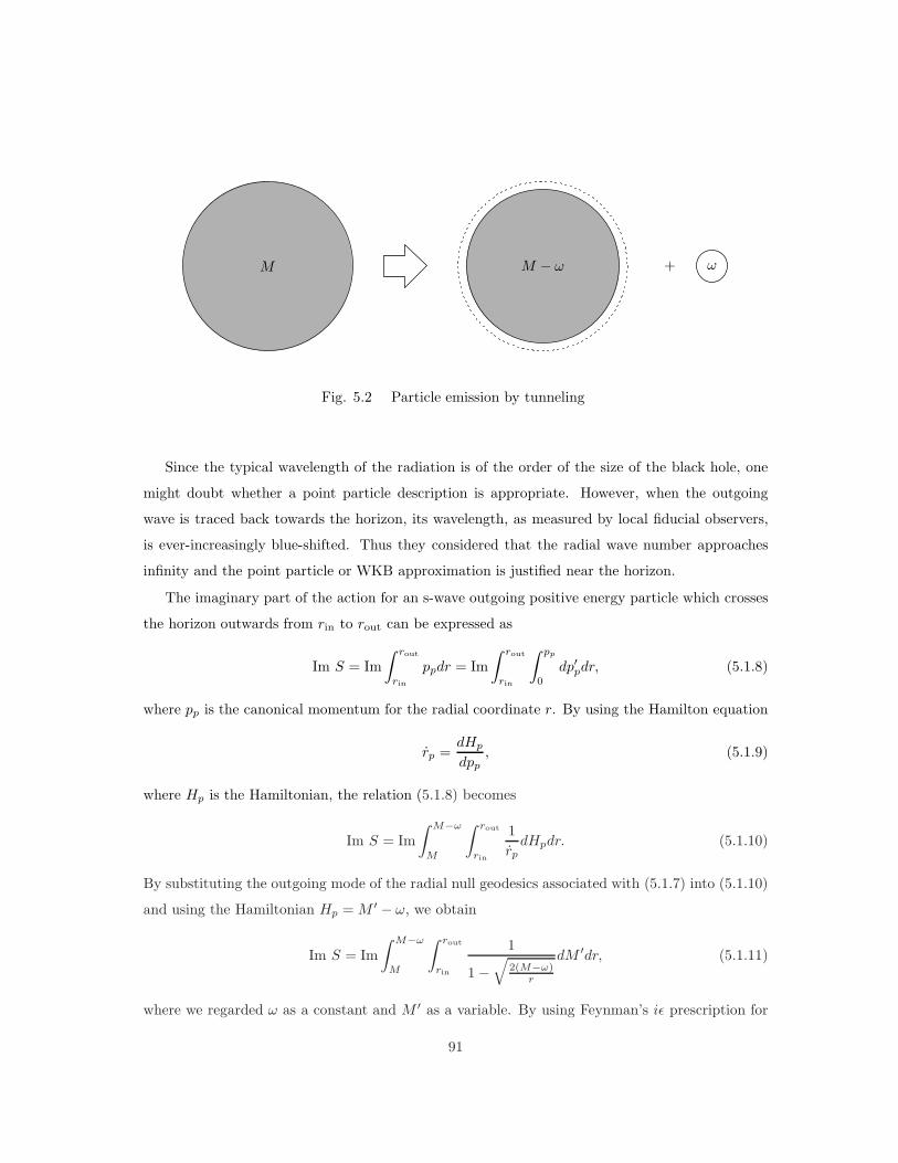
+M M − ω ω
Fig. 5.2 Particle emission by tunneling
Since the typical wavelength of the radiation is of the order of the size of the black hole, one
might doubt whether a point particle description is appropriate. However, when the outgoing
wave is traced back towards the horizon, its wavelength, as measured by local fiducial observers,
is ever-increasingly blue-shifted. Thus they considered that the radial wave number approaches
infinity and the point particle or WKB approximation is justified near the horizon.
The imaginary part of the action for an s-wave outgoing positive energy particle which crosses
the horizon outwards from rin to rout can be expressed as
Im S = Im
∫ rout
rin
ppdr = Im
∫ rout
rin
∫ pp
0
dp′pdr, (5.1.8)
where pp is the canonical momentum for the radial coordinate r. By using the Hamilton equation
rp =dHp
dpp, (5.1.9)
where Hp is the Hamiltonian, the relation (5.1.8) becomes
Im S = Im
∫ M−ω
M
∫ rout
rin
1
rpdHpdr. (5.1.10)
By substituting the outgoing mode of the radial null geodesics associated with (5.1.7) into (5.1.10)
and using the Hamiltonian Hp =M ′ − ω, we obtain
Im S = Im
∫ M−ω
M
∫ rout
rin
1
1−√
2(M−ω)r
dM ′dr, (5.1.11)
where we regarded ω as a constant and M ′ as a variable. By using Feynman’s iǫ prescription for
91

positive energy solutions ω → ω − iǫ, we obtain M →M − iǫ and
Im S = Im
∫ M−ω
M
∫ rout
rin
1
1−√
2M ′
r+ iǫ
dM ′dr (5.1.12)
= Im
∫ rout
rin
P1
1−√
2M ′
r
+
∫ M−ω
M
−iπδ(
1−√
2M ′
r
)
dM ′
dr, (5.1.13)
where P stands for the principal value. We can ignore the first term because it is a real part.
Now since the mass ranges from M to M − ω, the radial coordinate ranges from rin = 2M to
rout = 2(M − ω). Thus we can obtain the imaginary part of the action
Im S =
∫ rout
rin
∫ M−ω
M
−πδ(
1−√
2M ′
r
)
dM ′dr (5.1.14)
=
∫ 2(M−ω)
2M
(−πr)dr (5.1.15)
= 4πωM − 2πω2. (5.1.16)
The radially inward motion has a classically forbidden trajectory because the apparent horizon is
itself contracting. Thus, the limits on the integral indicate that, over the course of the classically
forbidden trajectory, the outgoing particle starts from r = 2M−ǫ, just inside the initial position of
the horizon, and traverses the contracting horizon to materialize at r = 2(M −ω)+ ǫ, just outside
the final position of the horizon (Fig. 5.3).
ǫ
2M
ǫ
2(M − ω)
BH
2ω
BH
Fig. 5.3 The contracting horizon
By using (5.1.16), we find the semi-classical WKB probability as
Γ ∼ e−2Im S = e−8πωM+4πω2
. (5.1.17)
92

Note that the probability is given by an absolute square of the amplitude. When we can ignore
the quadratic term of ω in the case of M ≫ ω, the probability (5.1.17) can be written as
Γ ∼ e−8πωM = e−2πωκ , (5.1.18)
where we used the surface gravity of the Schwarzschild black hole κ =1
4M. Here we recall
thermodynamics. It is well known that the Boltzmann factor in a thermal equilibrium state at a
temperature T is given by
ΓB = e−ωT . (5.1.19)
By comparing between (5.1.18) and (5.1.19), we find that the temperature of the black hole is
obtained by
TBH =κ
2π. (5.1.20)
This result agrees with the result of previous works as in (3.1.75).
5.2 Tunneling Mechanism in the Canonical Theory
The tunneling mechanism by Parikh andWilczek is explicit and straightforward in the canonical
theory. In this subsection, we would like to review the method of Parikh and Wilczek by using the
canonical theory.
To begin with, we consider the action of the system. The action is defined by
S =
∫
Ldt = −µm
∫
ds =
∫
−µm
ds
dtdt, (5.2.1)
where L is Lagrangian defined by
L = −µm
ds
dt, (5.2.2)
and µm is a mass of a particle. It is convenient to take the time component of the Painleve metric
positive, namely,
ds2 =
(
1− 2M
r
)
dt2p − 2
√
2M
rdtpdr − dr2, (5.2.3)
where the Painleve time tp is defined by
tp = t+ 2√2Mr + 2M ln
(√r −
√2M
√r +
√2M
)
, (5.2.4)
93

and t is the Schwarzschild time. From the metric (5.2.3), we obtain
ds
dtp= ±
√
(
1− 2M
r
)
− 2
√
2M
r
dr
dtp−(
dr
dtp
)2
, (5.2.5)
where we adopt +. We thus obtain the Lagrangian
Lp(r, rp) = −µm
√
(
1− 2M
r
)
− 2
√
2M
rrp − r2p, (5.2.6)
where rp ≡ dr
dtp. The canonical momentum for the radial coordinate r is defined by
pp ≡ ∂Lp
∂rp=
µm
(
rp +√
2Mr
)
√
1−(
rp +√
2Mr
)2, (5.2.7)
and by solving for rp, we obtain
rp = ±√
p2pp2p + µ2
m
−√
2M
r, (5.2.8)
where +(−) represents the outgoing (ingoing) mode. We adopt +, because we consider the outgoing
mode.
In canonical theory, the Hamiltonian is defined by
H = pr − L(r, r). (5.2.9)
By substituting (5.2.8) into (5.2.9), we obtain
Hp(r, pp) = pp
(√
p2pp2p + µ2
m
−√
2M
r
)
+ µm
√
µ2m
p2p + µ2m
. (5.2.10)
In the derivation of Parikh and Wilczek, they used the null geodesic equation. This can be
reproduced by taking µm = 0 in (5.2.8). By substituting µm = 0 into the Hamiltonian (5.2.10)
and solving for pp, we obtain
pp =Hp
1−√
2Mr
. (5.2.11)
From both (5.2.9) and (5.2.11), the action (5.2.1) is written as
S =
∫
Lpdtp =
∫
[pprp −Hp] dtp =
∫
ppdr −∫
Hpdtp =
∫
Hp
1−√
2Mr
dr −∫
Hpdtp. (5.2.12)
94

Now since the metric is stationary, it has a time-like Killing vector and there exists an energy as
the corresponding conserved quantity. The energy is defined as ω and it is the eigenvalue of the
Hamiltonian Hp = ω. The action (5.2.12) is written as
S =
∫ rout
rin
ω
1−√
2Mr
dr −∫ tp(out)
tp(in)
ωdtp. (5.2.13)
Now, we consider that an outgoing positive energy particle arising by the pair creation at rin close
to the horizon inside the black hole, appears at rout close to the horizon outside the black hole
through the horizon rH = 2M . The Painleve-time coordinates corresponding to these coordinates
are respectively defined as tp(in) and tp(out).
Since Hawking radiation is a quantum effect, we have only to evaluate the classically hidden
action i.e., the imaginary part of the action
Im S = Im
∫ rout
rin
ω
1−√
2Mr
dr. (5.2.14)
In the second term of (5.2.13), the Painleve-time coordinate is finite on the horizon and it has no
discontinuous point between tp(in) and tp(out). This can be understood from a naive discussion that
the Painleve coordinate can be kept to finite values even by substituting the future event horizon
(t, r) = (+∞, 2M) into (5.2.4). We can ignore the second term in (5.2.13) because it gives the real
part only. Since the first term in (5.2.13) is singular at the horizon r = 2M , there is a possibility
that the imaginary part appears, and we need to evaluate it.
By using the Feynman’s iǫ prescription for a real particle, we can obtain
Im S = Im
∫ rout
rin
ω
1−√
2Mr
− iǫdr (5.2.15)
= Im
Pω
1−√
2Mr
+ iπω
∫ rout
rin
δ
(
1−√
2M
r
)
dr
(5.2.16)
= 4πωM, (5.2.17)
where P stands for the principal value (the real part). This result agrees with (5.1.16) to the first
order.
95

5.3 Hawking Black Body Spectrum from Tunneling Mech-
anism
A method of deriving Hawking radiation based on quantum tunneling was originally proposed
by Parikh and Wilczek [7]. After Parikh and Wilczek’s derivation, a lot of papers on the tunneling
mechanism have been published. However the analysis has been confined to obtain the Hawking
temperature only by comparing the tunneling probability of an outgoing particle with the Boltz-
mann factor. The discussion of the spectrum was not transparent. Therefore, there remains the
possibility that the black hole is not the black but merely the thermal body. In this sense the tun-
neling method, presented so far, is not satisfactory yet. This problem was emphasized by Banerjee
and Majhi [8]. They showed how to reproduce the black body spectrum with the Hawking tem-
perature directly from the expectation value of number operator by using the properties of the
tunneling mechanism. Thus the derivation by the tunneling mechanism became more satisfactory.
In this subsection, we would like to review Banerjee and Majhi’s method [8]. For sake of
simplicity, we consider the case of a Schwarzschild black hole background. The metric is then
given by
ds2 = −f(r)dt2 + 1
f(r)dr2 + r2dΩ2, (5.3.1)
where f(r) is defined by
f(r) ≡ 1− 2M
r. (5.3.2)
We would like to note that they used not the Painleve metric (5.1.4) but the Schwarzschild metric
(5.3.1).
Here we consider the Klein-Gordon equation for a massless scalar field
gµν∇µ∇νφ = 0, (5.3.3)
where ∇µ is the covariant derivative defined by (3.1.8) and (3.1.9). By using the (r − t) sector of
the metric (5.3.1) in (5.3.3),
ds2 = −f(r)dt2 + 1
f(r)dr2, (5.3.4)
we obtain[
1
f(r)∂2t − f(r)∂2r − f ′(r)∂r
]
φ = 0. (5.3.5)
96

Taking the standard WKB ansatz
φ(r, t) = ei~S(r,t), (5.3.6)
and substituting the expansion for S(r, t) in terms of the Planck constant ~
S(r, t) = S0(r, t) +
∞∑
i=1
~iSi(r, t), (5.3.7)
in (5.3.5) where we write the Planck constant explicitly, we obtain, in the semiclassical limit (i.e.,
keeping only S0),
∂tS0(r, t) = ±f(r)∂rS0(r, t). (5.3.8)
Now we consider the classical Hamilton-Jacobi equation
∂S0
∂t+H = 0, (5.3.9)
where S0 is the classical action and H is the Hamiltonian. Since the metric (5.3.4) is stationary,
it has a timelike Killing vector. Thus the Hamiltonian is given by
H = ω, (5.3.10)
where ω is a constant and the conserved quantity corresponding to the timelike Killing vector.
This is identified as the effective energy experienced by the particle at asymptotic infinity. By the
Hamilton-Jacobi equation (5.3.9), we obtain
S0 = −ωt+ S0(r), (5.3.11)
where S0(r) is a time-independent arbitrary function. By substituting (5.3.11) into (5.3.8), we
obtain
ω = ±f(r)∂rS0(r). (5.3.12)
By using the relation of the tortoise coordinate defined by (2.2.6),
∂r∗ = f(r)∂r, (5.3.13)
the Hamilton-Jacobi equation (5.3.12) becomes
∂r∗S0(r) = ±ω. (5.3.14)
97
By integrating (5.3.14) over r∗, we obtained
S0(r) = ±ωr∗ + C, (5.3.15)
where C is an integration constant and we ignore it since it is included in a normalization constant
of the wave function. By substituting this into (5.3.11), the classical action becomes
S0(r, t) = −ω(t∓ r∗). (5.3.16)
Thus we can obtain the semiclassical solution for the scalar field
φ(r, t) = exp
[
− i
~ω(t∓ r∗)
]
. (5.3.17)
Here we introduce both the retarded time u and the advanced time v defined by (2.2.9),
u ≡ t− r∗, v ≡ t+ r∗, (5.3.18)
where we can regard u (v) as the outgoing (ingoing) modes of particles. We can then separate
the scalar field (5.3.17) into the ingoing (left handed) modes and outgoing (right handed) modes.
Since the tunneling effect is the quantum effect arising within the Planck length in the near horizon
region, we have to consider both the inside and outside regions which are very close to the horizon.
In the regions r+ − ε < r < r+, and r+ ≤ r < r+ − ε, respectively, we express the field φ as
φRin = exp
(
− i
~ωuin
)
φLin = exp
(
− i
~ωvin
)
(r+ − ε < r < r+), (5.3.19)
φRout = exp
(
− i
~ω′uout
)
φLout = exp
(
− i
~ω′vout
)
(r+ < r < r+ + ε), (5.3.20)
where ε is an arbitrarily small constant, “R (L)” stands for the right (left) modes and “in (out)”
stands for the inside (outside) of the black hole, respectively (Fig. 5.4). Here we note that these
fields are defined both in the inside and outside regions which are very close to the horizon.
98

BH outside
φLout φRout
inside
φLin φRin
εε
Horizon r+ + εr+ − ε
Fig. 5.4 Intuitive picture of the scalar field near the horizon
Now we consider that the outgoing particles inside the black hole quantum mechanically tunnel
through the horizon. However, it is well known that both the Schwarzschild coordinates (t, r)
and the Eddington-Finkelstein coordinates (u, v) are singular at the horizon. To describe horizon-
crossing phenomena, Parikh and Wilczek used the Painleve coordinates which have no singularity
at the horizon as already stated in Subsection 5.1. On the other hand, Banerjee and Majhi used
the Kruskal-Szekeres coordinates defined by
T =( r
2M− 1)
12
er
4M sinh
(
t
4M
)
R =( r
2M− 1)
12
er
4M cosh
(
t
4M
)
when r > 2M, (5.3.21)
T =(
1− r
2M
)12
er
4M cosh
(
t
4M
)
R =(
1− r
2M
)12
er
4M sinh
(
t
4M
)
when r < 2M. (5.3.22)
It is well known that these coordinates also have no singularity at the horizon. The Kruskal time
T and radial R coordinates inside and outside the horizon are represented as
Tout = exp [κ(r∗)out] sinh (κtout)Rout = exp [κ(r∗)out] cosh (κtout)
, (5.3.23)
Tin = exp [κ(r∗)in] cosh (κtin)Rin = exp [κ(r∗)in] sinh (κtin)
, (5.3.24)
where we used the tortoise coordinates as in (2.2.8) and the surface gravity of the Schwarzschild
black hole (3.1.52) in both (5.3.21) and (5.3.22).
99

In general, the Schwarzschild metric describes the behavior outside the black hole. Conse-
quently, the readers may wonder if these metrics defined by the Kruskal-Szekeres coordinates can
really describe the behavior inside the black hole. In our case, however, we study the tunneling
effect across the horizon and thus we study the behavior in the very small regions near the horizon.
In such an analysis, due to the reasons of continuity, it may not be unnatural to assume that the
Kruskal-Szekeres coordinates (5.3.23) and (5.3.24) can be used in both of outside and inside regions
of near the horizon. We note that these coordinates was used in the description of the Penrose
diagram as already stated in Subsection 2.2.
A set of coordinates (5.3.24) are connected with the other coordinates (5.3.23) by the relations,
tin → tout − iπ
2κ, (r∗)in → (r∗)out + i
π
2κ, (5.3.25)
so that, with this mapping, Tin → Tout and Rin → Rout smoothly. Following the definition (5.3.18),
we obtain the relations connecting the null coordinates defined inside and outside the horizon,
uin ≡ tin − (r∗)in → uout − iπ
κ, (5.3.26)
vin ≡ tin + (r∗)in → vout. (5.3.27)
This mapping is not defined if these coordinates are restricted to be real numbers. However, we
can define it by extending these coordinates to complex numbers as in (5.3.25) and (5.3.26). We
regard the appearance of the complex coordinates as a manifestation of quantum tunneling. In
analogy to the quantum tunneling in ordinary quantum mechanics, our picture is that the inside
solutions (5.3.19) and the outside solutions (5.3.20) of the infinitely high but very thin barrier,
which is located on top of the horizon, are connected via the complex coordinates (i.e., tunneling);
the precise connection of two coordinates is determined by asking the smooth connection of the
Kruskal-Szekeres coordinates at the horizon. Under these transformations the inside and outside
modes are connected by,
φRin ≡ exp
(
− i
~ωuin
)
→ exp(
−πω~κ
)
φRout, (5.3.28)
φLin ≡ exp
(
− i
~ωvin
)
→ φLout, (5.3.29)
where exp(
−πω~κ
)
of (5.3.28) stands for the effect of the tunneling mechanism. We would like
to note that these scalar fields are still identified with Schrodinger amplitude for a single particle
state. Therefore, the squared absolute value of the wave function represents the probability. The
100

probability of the tunneling effect is given by
Γ = exp
(
−2πω
~κ
)
. (5.3.30)
We find that this result in the natural system of units ~ = 1 agrees with Parikh and Wilczek’s
result as in (5.1.18).
To find the black body spectrum and the Hawking flux, Banerjee and Majhi considered n
number of non-interacting virtual pairs that are created inside the black hole. According to quan-
tum field theory, a wave function of one-particle system φ is related to the second-quantized field
operator ψ by
φ = 〈0|ψ|ω〉. (5.3.31)
By following the approach of Banerjee and Majhi [8], each of these pairs is represented by the
modes defined in the first set of (5.3.19) and (5.3.20). Then they defined the physical state of the
system, observed from outside, as
|Ψ〉 = N∑
n
|nLin〉 ⊗ |nR
in〉, (5.3.32)
where |nL(R)in 〉 is the number state of left (right) going modes inside the black hole and N is a
normalization constant. From the transformations of both (5.3.28) and (5.3.29), we obtain
|Ψ〉 = N∑
n
e−πnω~κ |nL
out〉 ⊗ |nRout〉. (5.3.33)
Here N can be determined by using the normalization condition 〈Ψ|Ψ〉 = 1. It is natural to
determine the normalization constant N for the state outside the black hole, because the observer
exists outside the black hole. Thus we obtain
N =1
(
∑
n
e−2πnω~κ
)12
. (5.3.34)
For bosons (n = 0, 1, 2, · · · ), N(boson) is calculated as
N(boson) =(
1− e−2πω~κ
)12
. (5.3.35)
For fermions (n = 0, 1), N(fermion) is similarly calculated as
N(fermion) =(
1 + e−2πω~κ
)− 12
. (5.3.36)
101

By substituting (5.3.35) or (5.3.36) into (5.3.33), we obtain the normalized physical states of a
system of bosons or fermions
|Ψ〉(boson) =(
1− e−2πω~κ
)12∑
n
e−πnω~κ |nL
out〉 ⊗ |nRout〉, (5.3.37)
|Ψ〉(fermion) =(
1 + e−2πω~κ
)− 12∑
n
e−πnω~κ |nL
out〉 ⊗ |nRout〉. (5.3.38)
From here on this analysis will be only for bosons since the analysis for fermions is identical. For
bosons, the density matrix operator of the system is given by
ρ(boson) ≡|Ψ〉(boson)〈Ψ|(boson)
=(
1− e−2πω~κ
)
∑
n,m
e−πω~κ
(n+m)|nLout〉 ⊗ |nR
out〉〈mRout| ⊗ 〈mL
out|. (5.3.39)
By tracing out the left going modes, we obtain the reduced density matrix for the right going
modes,
ρ(R)(boson) = Tr
(
ρ(R)(boson)
)
(5.3.40)
=∑
n
〈nLout|ρ(boson)|nL
out〉 (5.3.41)
=(
1− e−2πω~κ
)
∑
n
e−2πnω~κ |nR
out〉〈nRout|. (5.3.42)
Therefore the average number of particles detected at asymptotic infinity is given by
〈n〉boson = Tr(
nρ(R)(boson)
)
(5.3.43)
=(
1− e−2πω~κ
)
∑
n
ne−2πnω~κ (5.3.44)
=(
1− e−2πω~κ
)
(
−~κ
2π
)
∂
∂ω
(
∞∑
n=0
e−2πnω~κ
)
(5.3.45)
=(
1− e−2πω~κ
)
(
−~κ
2π
)
∂
∂ω
(
1
1− e−2πω~κ
)
(5.3.46)
=1
e2πω~κ − 1
, (5.3.47)
where the trace is taken over all |n(R)out 〉 eigenstates. This result in the natural system of units
(~ = 1) agrees with the result of Hawking’s original derivation as in (3.1.70). Similar analysis for
fermions leads to the Fermi distribution given by
〈n〉fermion =1
e2πω~κ + 1
. (5.3.48)
102

Correspondingly, the Hawking flux FH can be obtained by integrating the above distribution func-
tions over all ω’s. By following the discussion in Subsection 5.4.3, we would like to evaluate the
Hawking flux for fermions here. It is given by
FH =1
π
∫ ∞
0
ω
e2πω~κ + 1
dω =~2κ2
48π=
π
12β2, (5.3.49)
where we used
β ≡ 1
TBH
≡ 2π
~κ. (5.3.50)
This result agrees with the case of a = 0 in (4.3.32), i.e., the second term of (4.3.32).
Thus Banerjee and Majhi directly showed how to reproduce the black body spectrum and the
Hawking flux with the Hawking temperature from the expectation value of the number operator
by using the properties of the tunneling mechanism. Therefore, it is shown that black holes are
not merely the thermal body but the black body in the derivation from the tunneling mechanism.
In this sense, it may be said that the derivation on the basis of the tunneling mechanism became
more satisfactory.
5.4 Hawking Radiation from Kerr-Newman Black Hole and
Tunneling Mechanism
A variant of the approach to the derivation of Hawking radiation from the tunneling mechanism
was suggested by Banerjee and Majhi [8] as described in the preceding section. However, as stated
in their paper, their result is valid only for black holes with spherically symmetric geometry such
as Schwarzschild or Reissner-Nordstrom black holes in the 4-dimensional theory. According to the
black hole uniqueness theorem (see Section 2.1), 4-dimensional black holes have not only a mass
and a charge but also angular momentum. In 4 dimensions, the Kerr-Newman black hole, which
has both the charge and angular momentum, is the most general black hole and its geometry
becomes spherically asymmetric because of its own rotation. There exist several previous works
on a rotating black hole in the framework of the tunneling method (see for example [103–107]),
but they are mathematically very involved.
In this section, we would like to extend the method of Banerjee and Majhi based the tunneling
mechanism to the case of the Kerr-Newman black hole [9]. As shown in Section 2.4, we recall that
the 4-dimensional Kerr-Newman metric effectively becomes a 2-dimensional spherically symmetric
metric by using the technique of the dimensional reduction near the horizon. To the best of
103
my knowledge, there is no derivation of the spectrum by using the technique of the dimensional
reduction in the tunneling mechanism. Therefore, we believe that this derivation clarifies some
aspects of the tunneling mechanism. The essential idea is as follows: We consider the action for a
scalar field. We can then ignore the mass, potential and interaction terms in the action because the
kinetic term dominates in the high-energy theory near the horizon. By expanding the scalar field in
terms of the spherical harmonics and using properties at horizon, we find that the integrand in the
action dose not depend on angular variables. Thus we find that the 4-dimensional action with the
Kerr-Newman metric effectively becomes a 2-dimensional action with the spherically symmetric
metric.
We note that this technique is valid only for the region near the horizon. The use of the above
technique in the tunneling mechanism is justified since the tunneling effect is also the quantum
effect arising within the Planck length near the horizon region. By this procedure, the metric for
the Kerr-Newman black hole becomes an effectively 2-dimensional spherically symmetric metric,
and we can use the approach of Banerjee and Majhi which is valid for black holes with spherically
symmetric geometry. We can thus derive the black body spectrum and Hawking flux for the Kerr-
Newman black hole in the tunneling mechanism. We would like to suggest that the technique of
the dimensional reduction is also valid for Parikh and Wilczek’s original method in the tunneling
mechanism.
The contents of this section are as follows. In Subsection 5.4.1, we show how to define the
Kruskal-like coordinate for the effective 2-dimensional metric. In Subsection 5.4.2, we discuss the
tunneling mechanism for the case of a Kerr-Newman black hole. In Subsection 5.4.3, we show the
black body spectrum and the Hawking flux for the case of the Kerr-Newman black hole.
5.4.1 Kruskal-like coordinates for the effective 2-dimensional metric
In this subsection, we briefly explain that the 4-dimensional Kerr-Newman metric becomes a
2-dimensional spherically symmetric metric by using technique of the dimensional reduction near
the horizon. Then the Kruskal-like coordinates for the reduced metric are required instead of the
Kruskal-Szekeres coordinates for the 2-dimensional Schwarzschild metric as in (5.3.21) and (5.3.22).
We would like to show how to obtain the Kruskal-like coordinates from the reduced metric.
104

For a rotating and charged black hole, the metric is given by the Kerr-Newman metric (2.1.8)
ds2 =− ∆− a2 sin2 θ
Σdt2 − 2a sin2 θ
Σ(r2 + a2 −∆)dtdϕ
− a2∆sin2 θ − (r2 + a2)2
Σsin2 θdϕ2 +
Σ
∆dr2 +Σdθ2, (5.4.1)
where notations were respectively defined in Section 2.1. It follows from this expression that the
Kerr-Newman metric is spherically asymmetric geometry.
In the Kerr-Newman black hole background, the 4-dimensional action for a complex scalar field
is given by (2.4.1)
S =
∫
d4x√−ggµν(∂µ + ieVµ)φ
∗(∂ν − ieVν)φ+ Sint, (5.4.2)
where the first term is the kinetic term, the second term Sint represents the mass, potential and
interaction terms and Vµ is a gauge field associated with the Coulomb potential of the black hole.
By using the technique of the dimensional reduction near the horizon, it can be shown that the
4-dimensional action (5.4.2) becomes
S(H) = −∑
l,m
∫
dtdrΦφ∗lm
[
gtt (∂t − iAt)2+ ∂rg
rr∂r
]
φlm, (5.4.3)
as shown in (2.4.22). Then the effective metric near the horizon is given by (2.4.23)
ds2 = −f(r)dt2 + 1
f(r)dr2, (5.4.4)
where f(r) is defined by (2.4.10)
f(r) ≡ ∆
r2 + a2. (5.4.5)
We note that this function f(r) certainly contains the effect of the rotating black hole expressed by
a. From the form of (5.4.4), we find that a 4-dimensional Kerr-Newman metric (5.4.1) effectively
becomes the 2-dimensional spherically symmetric metric near the horizon. This expression also
shows that it is reasonable to consider only the (r − t) sector of the 4-dimensional metric and
massless particles without interactions, which were used in previous works [7, 8].
Banerjee and Majhi used Kruskal-Szekeres coordinates for a spherically symmetric metric such
as Schwarzschild or Reissner-Nordstrom metrics as in (5.3.23) and (5.3.24). In general, the concrete
forms of Kruskal-Szekeres coordinates for Schwarzschild or Reissner-Nordstrom metrics are well
known (as for the case of a Reissner-Nordstrom metric, for example, see §3.1 in [23]). In order to
105

extend Banerjee and Majhi’s method to the case of a Kerr-Newman black hole, we need to derive
the Kruskal-like coordinates for the effective reduced metric (5.4.4) following the derivation of the
Kruskal-Szekeres coordinates in the standard textbook. In this derivation, we apply a series of
coordinate transformations. Note that all the variables which appear in our transformations are
defined to be real numbers.
Now the metric is given by (5.4.4). By using (2.1.18), f(r) is also written as
f(r) =(r − r+)(r − r−)
r2 + a2, (5.4.6)
and r+(−) is the outer (inner) horizon given by (2.1.17).
As a first step of coordinate transformations, we use the tortoise coordinate defined by (2.4.10)
dr∗ ≡ 1
f(r)dr. (5.4.7)
The metric (5.4.4) is then written by
ds2 = −f(r)(dt− dr∗)(dt+ dr∗). (5.4.8)
By integrating (5.4.7) over r from 0 to r, we obtain
r∗ = r +1
2κ+ln
|r − r+|r+
+1
2κ−ln
|r − r−|r−
+ C, (5.4.9)
where κ+(−) is the surface gravity on the outer (inner) horizon and C is generally a pure imaginary
integration constant which appears in the analytic continuation. However, as already stated, we
would like to treat the case where all the variables (or parameters) are defined in the range of real
numbers. Thus we need to consider the three cases r > r+, r+ < r < r− and r− < r < 0 with
respect to the range of r. Actually, we have only to consider the two cases r > r+ and r+ < r < r−
because of the consideration near the outer horizon. When r > r+, the relation (5.4.9) becomes
r∗ = r +1
2κ+lnr − r+r+
+1
2κ−lnr − r−r−
. (5.4.10)
As the second step we use the retarded time u and the advanced time v defined by
u ≡ t− r∗ = t− r − 1
2κ+lnr − r+r+
− 1
2κ−lnr − r−r−
,
v ≡ t+ r∗ = t+ r +1
2κ+lnr − r+r+
+1
2κ−lnr − r−r−
.
when r > r+. (5.4.11)
The metric (5.4.8) is then written as
ds2 = −f(r)dudv. (5.4.12)
106

As the third step we use the following coordinate transformations U and V defined by
U ≡ −e−κ+u = −(
r − r+r+
)12(
r − r−r−
)
κ+2κ−
eκ+re−κ+t,
V ≡ eκ+v =
(
r − r+r+
)12(
r − r−r−
)
κ+2κ−
eκ+reκ+t.
when r > r+. (5.4.13)
The metric (5.4.12) is then written as
ds2 = −r+r−κ2+
e−2κ+r
r2 + a2
(
r−r − r−
)
κ+κ−
−1
dUdV. (5.4.14)
As the final step we use the following coordinate transformations T , R defined by
T ≡ 1
2(V + U) =
(
r − r+r+
)12(
r − r−r−
)
κ+2κ−
eκ+r sinh(κ+t),
R ≡ 1
2(V − U) =
(
r − r+r+
)12(
r − r−r−
)
κ+2κ−
eκ+r cosh(κ+t).
when r > r+. (5.4.15)
The metric (5.4.14) is then written as
ds2 =r+r−κ2+
e−2κ+r
r2 + a2
(
r−r − r−
)
κ+κ−
−1
(−dT 2 + dR2). (5.4.16)
Similarly, we consider the case of r+ > r > r−. When r+ > r > r−, the relation (5.4.9) becomes
r∗ = r +1
2κ+lnr+ − r
r++
1
2κ−lnr − r−r−
. (5.4.17)
As for the remaining coordinate transformations, we use the following ones
u ≡ t− r∗ = t− r − 1
2κ+lnr+ − r
r+− 1
2κ−lnr − r−r−
,
v ≡ t+ r∗ = t+ r +1
2κ+lnr+ − r
r++
1
2κ−lnr − r−r−
,
when r+ > r > r−, (5.4.18)
U ≡ e−κ+u =
(
r+ − r
r+
)12(
r − r−r−
)
κ+2κ−
eκ+re−κ+t,
V ≡ eκ+v =
(
r+ − r
r+
)12(
r − r−r−
)
κ+2κ−
eκ+reκ+t,
when r+ > r > r−, (5.4.19)
T ≡ 1
2(V + U) =
(
r+ − r
r+
)12(
r − r−r−
)
κ+2κ−
eκ+r cosh(κ+t),
R ≡ 1
2(V − U) =
(
r+ − r
r+
)12(
r − r−r−
)
κ+2κ−
eκ+r sinh(κ+t).
when r+ > r > r−. (5.4.20)
Of course, by performing these coordinate transformations, the corresponding metrics (5.4.12),
(5.4.14) and (5.4.16) do not change. The two sets of coordinates introduced here, both of (5.4.15)
107

and (5.4.20), are in fact the Kruskal-like coordinates. In the Schwarzshild case (a = Q = 0), (5.4.15)
and (5.4.20) respectively agree with (5.3.21) and (5.3.22). Finally, by rewriting the expressions
written in terms of r to the ones in terms of r∗ in the formulas (5.4.15) and (5.4.20), we obtain
T = exp [κ+r∗] sinh (κ+t)R = exp [κ+r∗] cosh (κ+t)
when r > r+, (5.4.21)
T = exp [κ+r∗] cosh (κ+t)R = exp [κ+r∗] sinh (κ+t)
when r+ > r > r−. (5.4.22)
These results agree with (5.3.23) and (5.3.24). Thus we can regard these coordinate variables as
the Kruskal-like coordinate variables for the effective reduced metric.
5.4.2 Tunneling mechanism
In this subsection, we discuss the connection between states inside and outside the black hole
to analyze the tunneling effect in the induced metric. We consider the Klein-Gordon equation near
the horizon. In Section 2.4, we showed that we can regard the 4-dimensional Kerr metric as the
2-dimensional spherically symmetric metric in the region near the horizon. As already stated, since
the kinetic term dominates in the high-energy theory near the horizon, we can ignore the mass,
potential and interaction terms. We obtain the Klein-Gordon equation with the gauge field from
the action (2.4.15)
[
1
f(r)(∂t − iAt)
2 − f(r)∂2r − f ′(r)∂r
]
φ = 0, (5.4.23)
where At is defined in (2.4.21) and f(r) is defined in (5.4.6). Of course, this equation can be
obtained from the general Klein-Gordon equation for a free particle with the gauge field in 2-
dimensional space-time
gµν(∇µ − iAµ)(∇ν − iAν)φ = 0, (5.4.24)
where ∇µ is the covariant derivative as in (3.1.7). In a manner similar to the procedure explained
in Section 5.3, we adopt the standard WKB ansatz
φ(r, t) = ei~S(r,t), (5.4.25)
and substituting the expansion of S(r, t)
S(r, t) = S0(r, t) +∞∑
i=1
~iSi(r, t), (5.4.26)
108

in (5.4.23), we obtain, in the semiclassical limit (i.e., keeping only S0),
∂tS0(r, t) = ±f(r)∂rS0(r, t). (5.4.27)
We find that terms including the gauge field vanished in the semiclassical limit. This equation
completely agrees with the equation in [8] although the content of f(r) is different from that used
in [8]. From the Hamilton-Jacobi equation as in (5.3.9) and (5.4.27), we obtain
S0(r, t) = − (ω − eΦH −mΩH) (t± r∗) ≡ −ω′(t± r∗), (5.4.28)
where r∗ is the tortoise coordinate defined by (2.4.10), ω is the characteristic frequency; ΦH is the
electric potential defined by (2.1.25), and ΩH is the angular frequency on the horizon respectively
defined by (2.1.24),
ΦH =Qr+
r2+ + a2, ΩH =
a
r2+ + a2. (5.4.29)
We also used the fact that the Hamiltonian is asymptotically given by
H = ω − eΦH −mΩH. (5.4.30)
Thus we obtain the semiclassical solution for the scalar field
φ(r, t) = exp
[
− i
~ω′(t± r∗)
]
. (5.4.31)
If one considers the metric at all regions for the charged and rotating black hole, the exterior
metric of the horizon is given by the 4-dimensional Kerr-Newman metric (5.4.1). However, we
showed that the metric near the horizon can be regarded as the 2-dimensional spherically symmetric
metric as in (5.4.4). We thus use the metric (5.4.4) in the region near the horizon. But we do not
know the interior metric of the black hole. However, if the interior metric is smoothly connected
to the exterior metric through the horizon, we may be able to identify the interior metric near the
horizon to be the same as the exterior metric near the horizon. We thus suppose that the interior
metric near the horizon is given by (5.4.4). Furthermore, since the tunneling effect is the quantum
effect arising within the Planck length in the near horizon region, we have to consider both the
inside and outside regions which are very close to the horizon.
Here we use both the retarded time u and the advanced time v defined by
u ≡ t− r∗, v ≡ t+ r∗. (5.4.32)
109

We can then separate the scalar field (5.4.31) into the ingoing (left handed) modes and outgoing
(right handed) modes. In the regions r+ − ε < r < r+, and r+ ≤ r < r+ − ε, respectively, we
express the field φ as
φRin = exp
(
− i
~ω′uin
)
φLin = exp
(
− i
~ω′vin
)
(r+ − ε < r < r+), (5.4.33)
φRout = exp
(
− i
~ω′uout
)
φLout = exp
(
− i
~ω′vout
)
(r+ < r < r+ + ε), (5.4.34)
where ε is an arbitrarily small constant, “R (L)” stands for the right (left) modes and “in (out)”
stands for the inside (outside) of the black hole, respectively (see Fig. 5.4). Here we note that
these fields are defined both the inside and outside regions which are very close to the horizon. As
for the definition of the fields in the region close to the horizon, there are related discussions in the
literatures [113, 114].
As shown in Subsection 5.4.1, we use the Kruskal-like coordinate variables
Tout = exp [κ+(r∗)out] sinh (κ+tout)Rout = exp [κ+(r∗)out] cosh (κ+tout)
. (5.4.35)
Tin = exp [κ+(r∗)in] cosh (κ+tin)Rin = exp [κ+(r∗)in] sinh (κ+tin)
, (5.4.36)
Both of the relations (5.4.35) and (5.4.36) agree with the relations in [8].
In general, the Schwarzschild and Kerr-Newman metrics describe the behavior outside the black
hole. Consequently, the readers may wonder if these metrics defined by the Kruskal coordinates
can really describe the behavior inside the black hole. In our case, however, we study the tunneling
effect across the horizon and thus we study the behavior in the very small regions near the horizon.
In such analysis, due to the reasons of continuity, it may not be unnatural to assume that the
Kruskal coordinates (5.4.35) and (5.4.36) can be used in both of outside and inside regions of near
the horizon.
A set of coordinates (5.4.35) are connected with the other coordinates (5.4.36) by the relations,
tin → tout − iπ
2κ+, (r∗)in → (r∗)out + i
π
2κ+, (5.4.37)
so that, with this mapping, Tin → Tout and Rin → Rout smoothly. Following the definition (5.4.32),
110

we obtain the relations connecting the null coordinates defined inside and outside the horizon,
uin ≡ tin − (r∗)in → uout − iπ
κ+, (5.4.38)
vin ≡ tin + (r∗)in → vout. (5.4.39)
This mapping is not defined if these coordinates are restricted to be real numbers. However, we
can define it by extending these coordinates to complex numbers as in (5.4.37) and (5.4.38). We
regard the appearance of the complex coordinates as a manifestation of quantum tunneling. In
analogy to the quantum tunneling in ordinary quantum mechanics, our picture is that the inside
solutions (5.4.33) and the outside solutions (5.4.34) of the infinitely high but very thin barrier,
which is located on top of the horizon, are connected via the complex coordinates (i.e., tunneling);
the precise connection of two coordinates is determined by asking the smooth connection of the
Kruskal-like coordinates at the horizon. Under these transformations the inside and outside modes
are connected by,
φRin ≡ exp
(
− i
~ω′uin
)
→ exp
(
− πω′
~κ+
)
φRout, (5.4.40)
φLin ≡ exp
(
− i
~ω′vin
)
→ φLout. (5.4.41)
As already discussed by Banerjee and Majhi in [8], the essential idea of the tunneling mechanism is
that a particle-antiparticle pair is formed close to the horizon. This pair creation may arise inside
the black hole ( in the region close to the horizon ), since the space-time is locally flat. The ingoing
mode is trapped inside the horizon while the outgoing mode can quantum mechanically tunnel
through the horizon. The outgoing mode is then observed at infinity as the Hawking flux. We
find that the effect of the ingoing mode inside the horizon do not appear outside the horizon as in
(5.4.41) since vin changes to vout without an extra term under the transformation connecting the
null coordinates defined inside and outside the horizon as in (5.4.39). On the other hand, we find
that the effect of the outgoing mode inside the horizon appear with a non-negligible probability by
tunneling through the horizon quantum mechanically as in (5.4.40). This consideration agrees with
the concept of tunneling mechanism. Furthermore, we showed that we can treat the Kerr-Newman
metric as a 2-dimensional spherically symmetric metric with a 2-dimensional effective gauge field
just as in the case of the simplest Schwarzschild metric in the tunneling mechanism.
111

5.4.3 Black body spectrum and Hawking flux
In this subsection, we show how to derive the Hawking black body spectrum for a Kerr-Newman
black hole by following the approach of Banerjee and Majhi as shown in Section 5.3. First, we
consider n number of non-interacting virtual pairs that are created inside the black hole. Then the
physical state of the system is conventionally written as
|Ψ〉 = N∑
n
|nLin〉 ⊗ |nR
in〉, (5.4.42)
where |nL(R)in 〉 is the number state of left (right) going modes inside the black hole and N is a
normalization constant. From the transformations of both (5.4.40) and (5.4.41), we obtain
|Ψ〉 = N∑
n
e−πnω′
~κ+ |nLout〉 ⊗ |nR
out〉. (5.4.43)
Here N can be determined by using the normalization condition 〈Ψ|Ψ〉 = 1. It is natural to
determine the normalization constant N for the state outside the black hole, because the observer
exists outside the black hole. Thus we obtain
N =1
(
∑
n
e− 2πnω′
~κ+
)12
. (5.4.44)
For bosons (n = 0, 1, 2, · · · ), N(boson) is calculated as
N(boson) =
(
1− e− 2πω′
~κ+
)12
. (5.4.45)
For fermions (n = 0, 1, 2), N(fermion) is also calculated as
N(fermion) =
(
1 + e− 2πω′
~κ+
)− 12
. (5.4.46)
By substituting (5.4.45) or (5.4.46) into (5.4.43), we obtain the normalized physical states of a
system of bosons or fermions
|Ψ〉(boson) =(
1− e− 2πω′
~κ+
)12 ∑
n
e−πnω′
~κ+ |nLout〉 ⊗ |nR
out〉, (5.4.47)
|Ψ〉(fermion) =
(
1 + e− 2πω′
~κ+
)− 12 ∑
n
e−πnω′
~κ+ |nLout〉 ⊗ |nR
out〉. (5.4.48)
112

Similarly to Section 5.3, we will present the analysis for bosons only. The density matrix operator
of the system is given by
ρ(boson) ≡|Ψ〉(boson)〈Ψ|(boson)
=
(
1− e− 2πω′
~κ+
)
∑
n,m
e− πω′
~κ+(n+m)
× |nLout〉 ⊗ |nR
out〉〈mRout| ⊗ 〈mL
out|. (5.4.49)
By tracing out the left going modes, we obtain the reduced density matrix for the right going
modes,
ρ(R)(boson) = Tr
(
ρ(R)(boson)
)
(5.4.50)
=∑
n
〈nLout|ρ(boson)|nL
out〉 (5.4.51)
=
(
1− e− 2πω′
~κ+
)
∑
n
e− 2πnω′
~κ+ |nRout〉〈nR
out|. (5.4.52)
Then, the expectation value of the number operator n is given by
〈n〉boson = Tr(
nρ(R)(boson)
)
(5.4.53)
=1
e2πω′
~κ+ − 1(5.4.54)
=1
eβ(ω−eΦ−mΩ) − 1(5.4.55)
where in the last line we used the definition (5.4.28) and we identify the Hawking temperature TBH
by
β ≡ 1
TBH≡ 2π
~κ+. (5.4.56)
This result corresponds to the black body spectrum with the Hawking temperature and agrees
with previous works in the Kerr-Newman black hole background [2]. Similar analysis for fermions
leads to the Fermi distribution
〈n〉fermion =1
eβ(ω−eΦ−mΩ) + 1. (5.4.57)
Moreover, the Hawking flux FH is derived by integrating the sum of the distribution function for a
particle with a quantum number (e, m) and its antiparticle with (−e, −m) over all ω’s. However, as
shown in Section 2.3, boson fields display the superradiance provided that they have frequency in a
113

certain range whereas fermion fields do not. We therefore evaluate the Hawking flux for fermions.
It is given by
FH =
∫ ∞
0
dω
2πω
[
1
eβ(ω−eΦ−mΩ) + 1+
1
eβ(ω+eΦ+mΩ) + 1
]
(5.4.58)
=π
12β2+
1
4π(eΦ+mΩ)2. (5.4.59)
This result agrees with the previous result [5] (see Appendix A in [5]).
One might be surprised by the sudden appearance of fermions. However, we can explicitly
present an answer to the question. As shown in Section 2.4, we know that the effective theory near
the horizon becomes a 2-dimensional theory. According to 2-dimensional quantum field theory,
it is known that there exists the boson-fermion duality [115]. Namely, the 2-dimensional boson
theory can be treated as the 2-dimensional fermion theory by the fermionization. We can also
discuss the tunneling mechanism for fermions in a manner similar to bosons.
Before closing, we discuss the black hole entropy. Since a particle emitted by the black hole
has the Hawking temperature, it is natural to consider that the black hole itself has the same
temperature. Thus we can obtain the black hole entropy dSBH from a thermodynamic consideration
dSBH =
(
dM
TBH
)
. (5.4.60)
By integrating Eq. (5.4.60), the entropy agrees with the Bekenstein-Hawking entropy
SBH =ABH
4~, (5.4.61)
where ABH is the surface area of the black hole
ABH = 4π(r2+ + a2). (5.4.62)
This result agrees with the Bekenstein-Hawking entropy (5.4.61). On the other hand, we defined
quantum states as in (5.4.42) and obtained the reduced density matrix as in (5.4.52). We can
evaluate the entropy for these states by using the von Neumann entropy formula. However, we
must mention that it is not the entropy of the black hole itself but rather the entropy of the boson
field. Our method does not allow us to derive the entropy for a black hole with a finite temperature
by counting the number of quantum states associated with the black hole. We thus simply derived
the black hole entropy from thermodynamic considerations as in (5.4.60) following previous works.
The derivation of the black hole entropy by counting the number of black hole quantum states
remains as one of future problems.
114

Finally, we mention that further recent developments associated with this derivation are given
in [116–118].
115

116

Chapter 6
Discussion and Conclusion
In this thesis, we investigated the black hole radiation which is commonly called Hawking
radiation. Hawking radiation is one of very interesting phenomena where both of general relativity
and quantum theory play a role at the same time since Hawking radiation is derived by taking into
account the quantum effects in the framework of general relativity. Hawking radiation is widely
accepted by now because the same result is derived by several different methods. At the same
time, there remain several aspects which have yet to be clarified. We attempted to clarify some
arguments in previous works and present more satisfactory derivations of Hawking radiation.
In Chapter 2, we reviewed basic facts and various properties of black holes as the necessary
preparation to discuss Hawking radiation. We showed that both of the black hole solutions and
their types are given as a result of general relativity, and that Penrose diagrams are useful to
understand the global structure of black hole space-time; a part of energy can be extracted from
a rotating black hole by the Penrose process and the technique of the dimensional reduction plays
an important role to understand the behavior of matter fields near the event horizon. We also
discussed analogies between black hole physics and thermodynamics, and we explained a method
to derive the black hole entropy which was suggested by Bekenstein. In particular, to understand
the properties of black holes, it is very useful to consider black hole physics in terms of well-known
thermodynamics. However, the corresponding relationships are no more than analogies in classical
theory. If we would like to show the complete correspondence between black hole physics and
thermodynamics, namely, to show that black holes actually have entropy and temperature, we
need to explain black hole radiation. Although Bekenstein suggested that black holes can have
entropy, the complete corresponding relationships was not established because Bekenstein was not
able to explain the mechanism of black hole radiation.
117

In Chapter 3, we discussed several previous works on Hawking radiation. Hawking radiation
which is derived by using quantum effects in black hole physics. By following Hawking’s original
derivation, we calculated the expectation value of the particle number by using the Bogoliubov
transformations. As is well known, the result agrees with the black body spectrum with a certain
temperature. By defining the temperature as the black hole temperature, it is confirmed that a
black hole behaves as a black body and we can thus explain the black hole radiation. The existence
of black hole radiation implies that the Hawking area theorem is violated. However, the second
law of black hole physics holds in a suitably generalized form. From these considerations, we can
understand the complete corresponding relationships between black hole physics and thermody-
namics, and we find that the radiation-dominated tiny black hole will eventually evaporate at some
point. We also briefly reviewed some representative derivations of Hawking radiation and stated
that there remain some aspects to be clarified.
In Chapter 4, we discussed the derivation of Hawking radiation based on anomalies. The essen-
tial idea is as follows: We can divide the field associated with a particle into ingoing modes falling
toward the horizon and outgoing modes moving away from the horizon near the horizon. Since
none of ingoing modes at horizon are expected to affect the classical physics outside the horizon,
we ignore the ingoing modes. Anomalies then appear since the effective theory is chiral near the
horizon. Anomalies mean the symmetry breaking by the quantization, i.e., the corresponding con-
servation law is violated, and it is known that a source of energy is generated. We can consider that
this source of energy corresponds to the characteristic energy flux of Hawking radiation. Since both
of the anomalies and Hawking radiation are typical quantum effects, it is natural that Hawking
radiation is related to anomalies. A method of deriving Hawking radiation based on the consider-
ation of anomalies was first suggested by Robinson and Wilczek and generalized by Iso, Umetsu
and Wilczek. However, there remained some aspects to be clarified. We clarified some arguments
in previous works on this approach and presented a simple derivation of Hawking radiation from
anomalies. We showed how to derive the Hawking flux by using the Ward identities for covariant
currents and two physically-meaningful boundary conditions. This derivation has a merit that we
can potentially incorporate matter fields with mass and interactions away from the horizon.
In Chapter 5, we discussed the derivation of Hawking radiation on the basis of quantum tunnel-
ing. The basic idea of the tunneling mechanism is as follows: We imagine that a particle-antiparticle
pair is formed close to the horizon. The ingoing mode is trapped inside the horizon while the out-
going mode can quantum mechanically tunnel through the horizon and it is observed at infinity
118

as the Hawking flux. A method of deriving Hawking radiation based on the tunneling mechanism
was suggested by Parikh and Wilczek. In this derivation, the discussion of the spectrum was not
transparent. Recently, by using the tunneling mechanism, a method of deriving the black body
spectrum directly was suggested by Banerjee and Majhi. But, their derivation is valid only for
black holes with spherically symmetric geometry such as Schwarzschild or Reissner-Nordstrom
black holes. We extended the simple derivation of Hawking radiation by Banerjee and Majhi on
the basis of the tunneling mechanism to the case of the Kerr-Newman black hole. By using the
technique of the dimensional reduction near the horizon, it is shown that the 4-dimensional Kerr-
Newman metric effectively becomes a 2-dimensional spherically symmetric metric near the horizon.
The use of this technique in the tunneling mechanism is justified since the tunneling effect is also
the quantum effect arising near the horizon region. To discuss the behavior of matter fields near
the event horizon, we defined the Kruskal-like coordinates for the effective reduced metric. We
showed that our final result of the black hole radiation from a rotating black hole agrees with the
previous result which is based on more elaborate analyses of the tunneling mechanism.
In conclusion, we presented several arguments which clarify two of the recent derivations of
Hawking radiation based on anomalies and tunneling. To be specific, we presented a simple
derivation of Hawking radiation on the basis of anomalies, and we extended Banerjee and Majhi’s
tunneling mechanism to a Kerr-Newman black hole by using the technique of the dimensional re-
duction near the horizon. A unified interpretation of various derivations of the black hole radiation,
which include two derivations analyzed here, remains as an interesting problem.
119

Acknowledgements
I would like to thank my supervisor, Professor Kazuo Fujikawa, for teaching me the profound
aspects of physics and for helpful support and encouragement throughout my graduate study.
I also thank Professor Shigefumi Naka and Professor Shinichi Deguchi for a careful reading of
the manuscript and continuous encouragement. I am very grateful to Professor Katsuyoshi Tsai,
Professor Takashi Mishima and Doctor Takeshi Nihei for useful comments and encouragement. I
am also grateful to all the other members of elementary particles theory group at Nihon University
for many discussions and encouragement.
I am thankful to Professor Satoshi Iso and Doctor Hiroshi Umetsu for valuable discussions
and helpful comments. I am happy to thank Professor Rabin Banerjee, Doctor Shailesh Kulkarni,
Doctor Bibhas Ranjan Majhi, Doctor Sujoy Kumar Modak, Doctor Debraj Roy and other mem-
bers of S. N. Bose National Centre for Basic Sciences for their hospitality during my stay there
and for many useful discussions. I would like to appreciate my family and my friends for their
encouragement and helpful support.
Finally, I gratefully acknowledge the financial support by the Strategic Project for Academic
Research of Nihon University.
120

Appendix
A Killing Vectors and Null Hypersurfaces
In this appendix, we review basic properties of both Killing vectors and null hypersurfaces.
To begin with, we discuss Killing vectors. On a 3-dimensional spacelike hypersurface Σ, the total
energy-momentum vector is given by
Pµ =
∫
Σ
T µνdΣν , (A.1)
where T µν is the energy-momentum tensor. This definition loses a physical meaning in the curved
space. In general, the global energy or momentum conservation laws cannot be maintained. How-
ever, when there exist particular vectors, the corresponding conservation laws can be maintained.
To find these laws, we consider a quantity given by
Pξ(Σ) =
∫
Σ
ξµTµνdΣν , (A.2)
where ξµ is an arbitrary vector. We note that this is a scalar quantity. Now, we consider the
volume V enclosed by two surfaces Σ and Σ′ (see Fig. 3.2 in Section 3.1). According to the Gauss
theorem, we obtain
Pξ(Σ′)− Pξ(Σ) =
∫
V
∇ν(ξµTµν)dV (A.3)
=
∫
V
[(∇νξµ)Tµν + ξµ(∇νT
µν)] dV (A.4)
=1
2
∫
V
(∇νξµ +∇µξν)TµνdV, (A.5)
where we used both the local conservation law of the energy-momentum tensor
∇νTµν = 0, (A.6)
and the fact that T µν is a symmetric tensor, i.e.,
(∇νξµ)Tµν =
1
2(∇νξµ +∇µξν)T
µν . (A.7)
If we choose the vector ξµ as that the vector satisfies
∇νξµ +∇µξν = 0, (A.8)
121

the quantity Pξ(Σ) is conserved, and we thus find that there is a corresponding symmetry in the
system. The particular vector and the corresponding equation (A.8) are respectively called the
“Killing vector” and the “Killing equation”. In other words, when there are symmetries in the
system, there exist the corresponding conserved quantities and the corresponding Killing vectors.
The conserved quantities are identified at asymptotic infinity.
Next we would like to discuss hypersurfaces. To begin with, we define S (x) as a smooth
function of the space-time coordinates xµ and consider a family of hyperspaces
S = constant. (A.9)
The vector normal to the hypersurface is given by
l = F (x) (gµν∂νS )∂
∂xµ, (A.10)
where F (r) is an arbitrary non-zero function. If the relation
l2 = 0, (A.11)
is satisfied for a particular hypersurface N , then N is called a “null hypersurface”.
As an example, we consider the case of Schwarzschild background. The metric is given by
ds2 = −(
1− 2M
r
)
dt2 +1
1− 2Mr
dr2 + r2dθ2 + r2 sin θdϕ2. (A.12)
By using the advanced time
v = t+ r∗, (A.13)
the Schwarzschild metric (A.12) in the ingoing Eddington-Finkelstein coordinates (v, r, θ, ϕ) is
rewritten as
ds2 = −(
1− 2M
r
)
dv2 + 2drdv + r2dΩ2. (A.14)
Then a surface is defined by
S = r − 2M. (A.15)
By substituting (A.15) into (A.10), we obtain
l = F (r)
[(
1− 2M
r
)
∂
∂r+
∂
∂v
]
, (A.16)
122

and
l2 = gµν∂µS ∂νSF 2(r) (A.17)
=
(
1− 2M
r
)
F 2(r). (A.18)
Thus we find that r = 2M is a null hypersurface and the relation (A.16) then becomes
l|r=2M = F (r)∂
∂v. (A.19)
Thus we find that interesting properties of null hypersurfaces as follows: We define N as a null
hypersurface with a normal vector l. A vector t which is tangent to N satisfies l · t = 0. However,
since N is null, the relation l · l = 0 is satisfied. Therefore, the vector l is itself a tangent vector,
i.e., we have
lµ =dxµ
dλ, (A.20)
where xµ(λ) is geodesic.
According to the definition of a Killing horizon, it is known that a Killing horizon is a null
hypersurface N with a Killing vector ξ which is normal to N .
B The First Integral by Carter
In this appendix, we show that the first integral is represented by
E2[r4 + a2(r2 + 2Mr −Q2)]− 2E(2Mr −Q2)apϕ − (r2 − 2Mr +Q2)p2ϕ − (µ2r2 + q)∆ = (pr∆)2
(B.1)
for the Kerr-Newman metric given by
ds2 =− ∆− a2 sin2 θ
Σdt2 − 2a sin2 θ
Σ(r2 + a2 −∆)dtdϕ
− a2∆sin2 θ − (r2 + a2)2
Σsin2 θdϕ2 +
Σ
∆dr2 +Σdθ2, (B.2)
where notations are the same as in Section 2.7. This derivation was first shown by Carter [45]. In
this derivation, he adopted the metric given by
ds2 =Σdθ2 − 2a sin2 θdrdϕ + 2drdu+1
Σ[(r2 + a2)2 −∆a2 sin2 θ] sin2 θdϕ2
− 2a
Σ(2Mr −Q2) sin2 θdϕdu−
[
1− 2Mr −Q2
Σ
]
du2, (B.3)
123

where u is the retarded time. This metric agrees with the Kerr-Newman metric (B.2) under the
transformations given by
du = dt+r2 + a2
∆dr
dϕ = dϕ+a
∆dr.
(B.4)
Carter considered the behavior of a particle with a mass µ and an electrical charge e in the
background with the metric (B.3). In this case, the general form of the Hamilton-Jacobi equation
is represented as
∂S
∂λ=
1
2gij[
∂S
∂xi− eAi
] [
∂S
∂xj− eAj
]
, (B.5)
where λ is an affine parameter associated with the proper time τ and defined by
τ ≡ µλ, (B.6)
Aµ stands for the gauge field (the electrical potential) and S is the Jacobi action. If there is a
separable solution, then in terms of the already known constants of the motion it must take the
form
S = −1
2µ2λ− Eu+ Lϕ+ Sθ + Sr, (B.7)
where E and L are given by
pu = −E, pϕ = L, (B.8)
where pµ stands for the momentum component in the direction of each coordinate variable. Here
Sθ and Sr are respectively functions of θ and r only. In this case, it can be shown that the first
integral is given by
p2θ +
(
aE sin θ − L
sin θ
)2
+ a2µ2 cos2 θ = K, (B.9)
∆p2r − 2[
(r2 + a2)E − aL+ eQr]
pr + µ2r2 = −K, (B.10)
where K is a constant.
Here we would like to know how the relations (B.9) and (B.10) are changed when we use the
Kerr-Newman metric (B.2) instead of the metric (B.3). Since we consider an electrically neutral
particle, we have e = 0. By differentiating (B.7), we obtain
dS = −1
2µ2dλ− Edu + Ldϕ+
(
∂Sθ
∂θ
)
dθ +
(
∂Sr
∂r
)
dr. (B.11)
124

Now we recall the transformations (B.4) which is used in order to derive the Kerr-Newman metric
from (B.3). By substituting (B.4) into (B.11), we obtain
dS = −1
2µ2dλ− E
(
dt+r2 + a2
∆dr
)
+ L(
dϕ+a
∆dr)
+
(
∂Sθ
∂θ
)
dθ +
(
∂Sr
∂r
)
dr
= −1
2µ2dλ− Edt+ Ldϕ+
(
∂Sθ
∂θ
)
dθ +
(
−r2 + a2
∆E +
a
∆Φ+
∂Sr
∂r
)
dr. (B.12)
Then the momenta conjugate to θ and r are given by
pθ =∂Sθ
∂θ, pr =
∂Sr
∂r. (B.13)
By using these relations, the relation (B.12) becomes
dS = −1
2µ2dλ− Edt+ Ldϕ+ pθdθ +
(
−r2 + a2
∆E +
a
∆L+ pr
)
dr. (B.14)
By comparing between (B.11) and (B.14), we find that a new radial momentum p′r is given by
p′r = pr −r2 + a2
∆E +
a
∆L, (B.15)
under the transformations (B.4). The relation (B.15) is also written as
pr = p′r +1
∆
[
(r2 + a2)E − aL]
. (B.16)
If the constant K in the relation (B.9) is rewritten as
K = q + (L− aE)2, (B.17)
we obtain
p2θ +(
aE sin θ − pϕsin θ
)2
+ a2µ2 cos2 θ = q + (pϕ − aE)2 (B.18)
⇔ q = cos2 θ
[
a2(µ2 − E2) +p2ϕ
sin2 θ
]
+ p2θ. (B.19)
Thus Carter’s kinetic constant is used in (2.6.26) in Section 2.6. By substituting (B.17) into (B.10),
we obtain
∆p2r − 2[(r2 + a2)E − aL]pr + µ2r2 = −q − p2ϕ + 2aEpϕ − a2E2. (B.20)
By using the transformation (B.16) in (B.20), we can obtain
∆
(
p′r +1
∆
[
(r2 + a2)E − apϕ]
)2
− 2[(r2 + a2)E − apϕ]
(
p′r +1
∆
[
(r2 + a2)E − apϕ]
)
+ µ2r2 + q + p2ϕ − 2aEpϕ + a2E2 = 0 (B.21)
⇔ E2[r4 + a2(r2 + 2Mr −Q2)]− 2E(2Mr −Q2)apϕ − (r2 − 2Mr +Q2)p2ϕ − (µ2r2 + q)∆ = (∆p′r)2
(B.22)
125

C Bogoliubov Transformations
In this appendix, we show that the Bogoliubov transformations (3.1.30) and (3.1.31),
bi =∑
j
(α∗ijaj − β∗
ija†j), (C.1)
b†i =
∑
j
(αija†j − βijaj), (C.2)
are the inverse transforms of (3.1.28) and (3.1.29) given by
ai =∑
j
(bjαij + b†jβ
∗ij), (C.3)
a†i =
∑
j
(bjβij + b†jα
∗ij). (C.4)
By substituting both (C.3) and (C.4) into the right-hand side of (C.1), we obtain
∑
j
(α∗ijaj − β∗
ija†j) (C.5)
=∑
j,k
[
α∗ij
(
αjkbk + β∗ikb
†k
)
− β∗ij
(
βjkbk + α∗ikb
†k
)]
(C.6)
=∑
k
∑
j
(
α∗ijαjk − β∗
ijβjk)
bk +∑
j
(
α∗ijβ
∗jk − β∗
ijα∗jk
)
b†k
. (C.7)
Now we recall the orthonormal condition (3.1.14) for fi and f∗i , i.e.,
ρ(fi, f∗j ) =
1
2i
∫
Σ
(fi∇µf∗j − f∗
j ∇µfi)dΣµ = δij , (C.8)
which implies the following relations
ρ(f∗i , fj) = −δij , (C.9)
ρ(fi, fj) = ρ(f∗i , f
∗j ) = 0. (C.10)
The orthonormal condition (3.1.25) for pi and p∗i is also satisfied
ρ(pi, p∗j ) = δij . (C.11)
By substituting the relations between pi and fi,
pi =∑
k
(αikfk + βikf∗k ), (C.12)
p∗j =∑
l
(α∗jlf
∗l + β∗
jlfl), (C.13)
126

into (C.11), we obtain
ρ(pi, p∗j ) = ρ
(
∑
k
(αikfk + βikf∗k ),
∑
l
(α∗jlf
∗l + β∗
jlfl))
)
(C.14)
=∑
k,l
[
αikα∗jlρ(fk, f
∗l ) + αikβ
∗jlρ(fk, fl) + βikα
∗jlρ(f
∗k , f
∗l ) + βikβ
∗jlρ(f
∗k , fl)
]
, (C.15)
By using (C.8), (C.9) and (C.10) in (C.15), we obtain
ρ(pi, p∗j ) =
∑
k,l
[
αikα∗jlδkl + βikβ
∗jl(−δkl)
]
(C.16)
=∑
k
(αikα∗jk − βikβ
∗jk). (C.17)
From (C.11), we thus obtain
∑
k
(
αikα∗jk − βikβ
∗jk
)
= δij . (C.18)
Similarly, when we consider the case of ρ(p∗i , p∗j ) = 0, we obtain
∑
k
(
β∗ikα
∗jk − α∗
ikβ∗jk
)
= 0. (C.19)
By substituting (C.18) and (C.19) into (C.7), we obtain
∑
k
∑
j
(
α∗ijαjk − β∗
ijβjk)
bk +∑
j
(
α∗ijβ
∗jk − β∗
ijα∗jk
)
b†k
=∑
k
δikbk (C.20)
= bi (C.21)
Thus we can reproduce bi from the right-hand side of (C.1). We can similarly calculate as for b†i .
Therefore we can confirm that the relations (C.1) and (C.2) are the inverse transforms of (C.3)
and (C.4).
D Solutions of Klein-Gordon Equation in Schwarzschild Space-
time
In this appendix, we show that the solutions of the Klein-Gordon equation, in (3.1.10)
gµν∇µ∇νφ = 0, (D.1)
127

are given by (3.1.39) and (3.1.40)
fω′lm =Fω′(r)
r√2πω′
eiω′vYlm(θ, ϕ), (D.2)
pωlm =Pω(r)
r√2πω
eiωuYlm(θ, ϕ). (D.3)
By using a property of the covariant derivative for a scalar field φ,
∇νφ = ∂νφ, (D.4)
the equation (D.1) becomes
∇µ (gµν∂νφ) = 0, (D.5)
where ∂ν and ∇µ respectively stand for an ordinary derivative and a covariant derivative. The
covariant derivative for a vector field Aµ is also given by
∇µAµ = ∂µA
µ + ΓµνµA
ν , (D.6)
where Γµνρ is the Christoffel symbol and Γµ
νµ is written as
Γµνµ =
1
2gµρ(∂µgρν + ∂νgρµ − ∂ρgνµ) (D.7)
=1
2(gµρ∂µgρν + gµρ∂νgρµ − gµρ∂ρgνµ). (D.8)
Since the third term is canceled by the first term by exchanging µ and ρ in the third term of (D.8),
the relation (D.8) becomes
Γµνµ =
1
2gµρ∂νgρµ. (D.9)
Now we would like to show that ∂νgρµ is given by
∂νgρµ = (ggρµ)−1 ∂νg, (D.10)
where g is defined by
g ≡ det (gµρ) . (D.11)
The definition (D.11) can also be written as
g = exp (ln det gµρ) (D.12)
= exp (Tr ln gµρ) . (D.13)
128

Then, the small variation of g is given by
δg = exp Tr [ln(gµρ + δgµρ)] − exp(Tr ln gµρ). (D.14)
By using the Taylor expansion for a matrix X
ln(X + δX) ≈ lnX +X−1δX, (D.15)
the relation (D.14) becomes
δg ≈ exp [Tr (ln gµρ + gµνδgνρ)]− exp [Tr(ln gµρ)] (D.16)
= exp [Tr(ln gµρ)] exp [Tr(gµνδgνρ)]− exp [Tr(ln gµρ)] . (D.17)
By performing the Taylor expansion for exp [Tr(gµνδgνρ)] and retaining the first order of terms,
we obtain
δg ≈ exp [Tr(ln gµρ)] (1 + Trgµνδgνρ)− exp [Tr(ln gµρ)] (D.18)
= exp [Tr(ln gµρ)] Tr(gµνδgνρ) (D.19)
= g · Tr(gµνδgνρ) (D.20)
= g · gµνδgνµ. (D.21)
By replacing ν to ρ in (D.21), we obtain
δg = g · gµρδgρµ. (D.22)
From this, we find
∂νg = g · gµρ∂νgρµ (D.23)
⇔ ∂νgρµ = (g · gµρ)−1∂νg. (D.24)
Thus we establish the relation (D.10).
By substituting (D.10) into (D.9), we obtain
Γµνµ =
1
2gµρ
1
g · gµρ ∂νg (D.25)
=1
2g∂νg. (D.26)
Since we have
1√−g∂ν(√−g) = 1
2g∂νg, (D.27)
129

the relation (D.26) becomes
Γµνµ =
1√−g∂ν(√−g). (D.28)
By substituting (D.28) into (D.6), we obtain
∇µAµ = ∂µA
µ +1√−g∂ν(
√−g)Aν (D.29)
By replacing ν by µ, the relation (D.29) becomes
∇µAµ =
1√−g∂µ(√−gAµ). (D.30)
Thus the Klein-Gordon equation (D.5) is written as
1√−g∂µ(√−g · gµν∂νφ) = 0. (D.31)
Since we consider physics in the Schwarzschild background, the metric is given by (2.1.7)
(gµν) =
−(
1− 2Mr
)
0 0 0
0(
1− 2Mr
)−10 0
0 0 r2 00 0 0 r2 sin2 θ
(D.32)
From this metric, g is given by
g = −r4 sin2 θ (D.33)
By substituting (D.32) and (D.33) into (D.31), the Klein-Gordon equation becomes
[
− r
r − 2M
∂2
∂t2+
1
r2∂
∂r
r2(
r − 2M
r
)
∂
∂r
− 1
r2
(
− ∂
∂θsin θ
∂
∂θ− 1
sin2 θ
∂2
∂ϕ2
)]
φ = 0. (D.34)
Here we define a quadratic angular momentum by
L2 ≡ − ∂
∂θsin θ
∂
∂θ− 1
sin2 θ
∂2
∂ϕ2. (D.35)
Then (D.34) is written as
[
− r
r − 2M
∂2
∂t2+
1
r2∂
∂r
r2(
r − 2M
r
)
∂
∂r
− 1
r2L2
]
φ = 0. (D.36)
Now we rewrite φ as
φ =(
Ae−iωt +A∗eiωt)
R(r)Θ(θ, ϕ). (D.37)
130

By substituting (D.37) into (D.36), we obtain[
− r
r − 2M(iω)2 +
1
r2∂
∂r
r2(
r − 2M
r
)
∂
∂r
− 1
r2L2
]
(
Ae−iωt +A∗eiωt)
R(r)Θ(θ, ϕ) = 0.
(D.38)
By dividing the both sides by(
Ae−iωt +A∗eiωt)
and transferring the third term to the right-hand
side, we obtain[
r
r − 2Mω2 +
1
r2∂
∂r
r2(
r − 2M
r
)
∂
∂r
]
R(r)Θ(θ, ϕ) =R(r)
r2L2Θ(θ, ϕ). (D.39)
By dividing the both sides byR(r)
r2Θ(θ, ϕ), the equation (D.39) becomes
r2
R(r)
[
r
r − 2Mω2 +
1
r2∂
∂r
r2(
r − 2M
r
)
∂
∂r
]
R(r) =1
Θ(θ, ϕ)L2Θ(θ, ϕ). (D.40)
Since (D.40) is represented in a separable form, the equation is set to be a constant. By writing
the constant as l(l + 1), we obtain
L2Θ(θ, ϕ) = l(l+ 1)Θ(θ, ϕ), (D.41)[
r
r − 2Mω2 +
1
r2∂
∂r
r2(
r − 2M
r
)
∂
∂r
− l(l+ 1)
r2
]
R(r) = 0. (D.42)
From (D.41), we can expand Θ(θ, ϕ) by
Θ(θ, ϕ) =∑
m
BlmYlm(θ, ϕ), (D.43)
where Blm is an integration constant and Ylm(θ, ϕ) stands for the spherical harmonics. In the
equation (D.42), we use the definition
R′(r∗) ≡ rR(r), (D.44)
where r∗ is the tortoise coordinate defined by
r∗ ≡ r + 2M ln∣
∣
∣
r
2M− 1∣
∣
∣ . (D.45)
Then for this transformation we
∂
∂r=
(
r
r − 2M
)
∂
∂r∗. (D.46)
Under these transformations, the equation (D.42) becomes
1
r
[
r
r − 2Mω2 +
(
r
r − 2M
)
∂2
∂r2∗− 2M
r3− 1
r2l(l+ 1)
]
R′(r∗) = 0. (D.47)
131

By dividing the both sides of (D.47) by1
r
(
r
r − 2M
)
, we obtain
∂2
∂r2R′(r∗) +
[
ω2 − 1
r2
2M
r+ l(l+ 1)
(
1− 2M
r
)]
R′(r∗) = 0. (D.48)
As stated in Section 3.1, the solutions fω′lm and pωlm are partial waves at r → ∞. Thus, by taking
r → ∞ in (D.48), we obtain
∂
∂r2∗R′(r∗) + ω2R′(r∗) = 0. (D.49)
The solution for this equation is given by
R′(r∗) = Cωle−iωr∗ + C∗
ωleiωr∗ , (D.50)
where Cωl is an integration constant. By substituting (D.44) into (D.50), we obtain
R(r) =1
r
(
Cωle−iωr∗ + C∗
ωleiωr∗
)
. (D.51)
By substituting both (D.43) and (D.51) into (D.37), we thus obtain
φ =∑
ω,l,m
1
r
(
ACωle−iω(t+r∗) +AC∗
ωle−iω(t−r∗) +A∗Cωle
iω(t−r∗) +A∗C∗ωle
iω(t+r∗))
BlmYlm(θ, ϕ).
(D.52)
We use affine parameters defined by
v ≡ t+ r∗, (D.53)
u ≡ t− r∗, (D.54)
where v and u are respectively called the advanced time and the retarded time. By putting together
the integration constants in (D.52) except for the normalization constant1√2πω
, which is often
used in the Klein-Gordon equation, we can thus write the partial waves as
fω′lm =Fω′(r)
r√2πω′
eiω′vYlm(θ, ϕ), (D.55)
pωlm =Pω(r)
r√2πω′
eiωuYlm(θ, ϕ), (D.56)
where we regarded Fω′(r) and Pω(r) as not integration constants but rather “integration variables”
which depend on r, because we want to take into account the small effect of r arising from the
approximation by setting r → ∞.
132

E Calculation of Bogoliubov Coefficients
The Bogoliubov coefficients αωω′ and βωω′ are given by (3.1.47) and (3.1.48)
αωω′ =r√ω′
√2πFω′
∫ ∞
−∞
dve−iω′vpω, (E.1)
βωω′ =r√ω′
√2πFω′
∫ ∞
−∞
dveiω′vpω. (E.2)
When the partial wave pω is represented as (3.1.55),
p(2)ω ∼
0, (v > v0),P−ω
r√2πω
exp
[
−iωκln
(
v0 − v
CD
)]
, (v ≤ v0),(E.3)
we show that the corresponding α(2)ωω′ and β
(2)ωω′ are given by (3.1.57) and (3.1.58), i.e.,
α(2)ωω′ ≈
1
2πP−ω (CD)
iωκ e−iω′v0
(√
ω′
ω
)
Γ
(
1− iω
κ
)
(−iω′)−1+ iωκ , (E.4)
β(2)ωω′ ≈ −iα(2)
ω(−ω′). (E.5)
To begin with, by substituting (E.3) into (E.1)
α(2)ωω′ =
r√ω′
√2πFω′(r)
∫ v0
−∞
dvPω(r)
r√2πω
exp
[
−iωκln
(
v0 − v
CD
)]
e−iω′v, (E.6)
where Fω′(r) and Pω(r) are integration variables which take into account the small effect of r, and
we collectively rewrote them as Pω(r). Since we now consider the region near the horizon r = 2M
we use P−ω ≡ Pω(2M). Thus the relation (E.6) becomes
α(2)ωω′ =
1
2πP−ω (CD)i
ωκ
√
ω′
ω
∫ v0
−∞
dv(v0 − v)−iωκ e−iω′v. (E.7)
By integrating over the variable defined as v0 − v = x, we obtain
α(2)ωω′ =
1
2πP−ω (CD)i
ωκ
√
ω′
ωe−iω′v0
∫ ∞
0
dxx−iωκ e−(−iω′)x. (E.8)
By using a formula of the gamma function,
Γ(ε)t−ε =
∫ ∞
0
dssε−1e−ts, (E.9)
we finally obtain (E.4),
α(2)ωω′ =
1
2πP−ω (CD)i
ωκ
√
ω′
ωe−iω′v0Γ(1 − i
ω
κ)(−iω′)1−iω
κ . (E.10)
Similarly, we can show the relation (E.5) for β(2)ωω′ .
133

134

Bibliography
[1] S.W. Hawking, Nature 248, 30 (1974).
[2] S.W. Hawking, Commun. Math. Phys. 43, 199 (1975).
[3] S.P. Robinson and F. Wilczek, Phys. Rev. Lett. 95, 011303 (2005).
[4] S. Iso, H. Umetsu and F. Wilczek, Phys. Rev. Lett. 96, 151302 (2006).
[5] S. Iso, H. Umetsu and F. Wilczek, Phys. Rev. D74, 044017 (2006).
[6] K. Umetsu, Prog. Theor. Phys. 119 849 (2008).
[7] M.K. Parikh and F. Wilczek, Phys. Rev. Lett. 85, 5042 (2000).
[8] R. Banerjee and B.R. Majhi, Phys. Lett. B675, 243 (2009).
[9] K. Umetsu, arXiv:0907.1420[hep-th].
[10] A. Einstein, Preuss. Akad. Wiss. Berlin, Sitzber. 778 (1915).
[11] A. Einstein, Preuss. Akad. Wiss. Berlin, Sitzber. 844 (1915).
[12] K. Schwarzschild, Sitzber. Deut. Akad. Wiss. Berlin, Kl. Math.-Phys. Tech., 189 (1916).
[13] W. Israel, Phys. Rev. 164, 1776 (1967).
[14] B. Carter, Phys. Rev. Lett. 26, 331 (1971).
[15] S.W. Hawking and G. F. R. Ellis, The Large Scale Structure of Space-Time, (Cambridge
University Press, 1975), §9.3.
[16] R. Ruffini and J.A. Wheeler, Phys. Today, 24, 30 (1971).
[17] R. Penrose, Riv. Nuovo Cim.1, 252, (1969).
135
[18] M. Banados, C. Teitelboim and J. Zanelli, Phys. Rev. Lett. 69, 1849 (1992).
[19] M. Banados, M. Henneaux, C. Teitelboim and J. Zanelli, Phys. Rev. D48, 1506 (1993).
[20] R.C. Myers and M.J. Perry, Ann. Phys. 172, 304 (1986).
[21] R. Emparan and H.S. Reall, Phys. Rev. D65, 084025 (2002).
[22] R. Penrose, Conformal treatment of infinity, in B. S. DeWitt and C. M. DeWitt eds, Relativity,
Groups and Topology,(Gordon and Breach, New York, 1964), 565.
[23] P.K. Townsend, arXiv: gr-qc/9707012.
[24] J.A. Wheeler, Phys. Rev. 97, 511 (1955).
[25] T. Regge and J.A. Wheeler, Phys. Rev. 108, 1063 (1957).
[26] A.S. Eddington, Nature 113, 192 (1924).
[27] D. Finkelstein, Phys. Rev. 110, 965 (1958).
[28] M.D. Kruskal, Phys. Rev. 119, 1743 (1960).
[29] G. Szekeres, Publ. Mat. Debrecen 7, 285 (1960).
[30] R. Penrose, Riv. Nuovo Cim. 1, 252 (1969).
[31] D. Christodoulou, Phys. Rev. Lett. 25, 1596 (1970).
[32] S.W. Hawking, Phys. Rev. Lett. 26, 1344 (1971).
[33] W.C. Misner, Phys. Rev. Lett. 28, 994 (1972).
[34] W.H. Press and S.A. Teukolsky, Nature 238, 211 (1972).
[35] W. Unruh, Phys. Rev. Lett. 31, 1265 (1973).
[36] R. Guven, Phys. Rev. D16, 1706 (1977).
[37] J.M. Greif, Junior thesis, Princeton University, unpublished (1969).
[38] J.D. Bekenstein, Phys. Rev. D7, 2333 (1973).
[39] J.M. Bardeen, B. Carter and S.W. Hawking, Commun. Math. Phys. 31, 161 (1973).
136

[40] R.M. Wald, General Relativity, (The University of Chicago Press, 1984), §12.5.
[41] C.E. Shannon, Bell Syst. Tech. J. 27, 379 (1948).
[42] C.E. Shannon and W. Weaver, The mathematical theory of communication, (Urbana: Univer-
sity of Illinois Press, 1949).
[43] L. Brillouin, Science and Information Theory, (Acad. Press, Inc., New York, 1956), §12.1.
[44] D. Christodoulou and R. Ruffini, Phys. Rev. D4, 3552 (1971).
[45] B. Carter, Phys. Rev. 174, 1559 (1968).
[46] J.D. Bekenstein, Lett. Nuovo Cim. 4, 737 (1972).
[47] W. Greiner, L. Neise and H. Stocker, THERMODYNAMICS AND STATISTICAL MECHAN-
ICS, (Springer-Verlag New York, Inc. 1995), Chapter 5.
[48] B.F. Schutz, A first course in general relativity, (Cambridge Univ. Press, 1985), §11.5.
[49] P.A. M. Dirac, General theory of relativity, (Princeton Univ. Press, 1996).
[50] B.S. DeWitt, Phys. Rept. C19, 295 (1975).
[51] S.W. Hawking, Mon. Not. Roy. Astron. Soc. 152, 75 (1971).
[52] B.J. Carr and S.W. Hawking, Mon. Not. Roy. Astron. Soc. 168, 399 (1974).
[53] J.D. Bekenstein, Phys. Rev. D9, 3292 (1974).
[54] S.W. Hawking, Commun. Math. Phys. 25, 152 (1972).
[55] G.W. Gibbons and S.W. Hawking, Phys. Rev. D15, 2752 (1977).
[56] L. Smarr, Phys. Rev. Lett. 30, 71 (1973); 30, 521 (1973)(E).
[57] M. Banados, C. Teitelboim and J. Zanelli, Phys. Rev. Lett. 72, 957 (1994).
[58] S.W. Hawking and G.T. Horowitz, Class. Quant. Grav. 13, 1487 (1996).
[59] S.M. Christensen and S.A. Fulling, Phys. Rev. D15, 2088 (1977).
[60] R.A. Bertlmann and E. Kohlprath, Ann. Phys 288, 137 (2001).
137

[61] K. Fujikawa, Phys. Rev. A79, 032334 (2009).
[62] K. Fujikawa, Phys. Rev. A80, 012315 (2009).
[63] M. Srednicki, Phys. Rev. Lett. 71, 666 (1993).
[64] S. Mukohyama, M. Seriu and H. Kodama, Phys. Rev. D55, 7666 (1997).
[65] H. Terashima, Phys. Rev. D61, 104016 (2000).
[66] A. Strominger and C. Vafa, Phys. Lett. B379, 99 (1996).
[67] C.G. Callan and J.M. Maldacena, Nucl.Phys. B472, 591 (1996).
[68] K. Murata and J. Soda, Phys. Rev. D74, 044018 (2006).
[69] E. Nother, Nachr. d. Koning. Gesellsch. d. Wiss. zu Gottingen, Math-phys. Klasse, 235 (1918).
(English translation by M.A. Tavel, arXiv: physics/0503066).
[70] H. Fukuda and Y. Miyamoto, Prog. Theor. Phys. 4, 49 (1949).
[71] J.S. Bell and R. Jackiw, Nuovo Cim. A60, 47 (1969).
[72] S.L. Adler, Phys. Rev. 177, 2426 (1969).
[73] K. Fujikawa, Phys. Rev. Lett. 42, 1195 (1979).
[74] K. Fujikawa, Phys. Rev. D21, 2848 (1980); D22, 1499 (1980)(E).
[75] K. Fujikawa and H. Suzuki, Path Integrals and Quantum Anomalies, (Oxford Univ. Press,
2004).
[76] R. Banerjee and S. Kulkarni, Phys. Rev. D77, 024018 (2008).
[77] J. Wess and B. Zumino, Phys. Lett. B37, 95 (1971).
[78] R. Banerjee and S. Kulkarni, Phys. Lett. B659, 827 (2008).
[79] A.M. Polyakov, Phys. Lett. B103, 207 (1981).
[80] H. Leutwyler, Phys. Lett. B153, 65 (1985).
[81] K. Fujikawa, Phys. Rev. Lett. 44, 1733 (1980).
138

[82] L. Alvarez-Gaume and E. Witten, Nucl. Phys. B234, 269 (1984).
[83] K. Fujikawa, M. Tomiya and O. Yasuda, Z. Phys. C28, 289 (1985).
[84] R. Bertlmann and E. Kohlprath, Ann. of Phys. 288, 137 (2001).
[85] G. ’t Hooft, Phys. Rev. Lett. 37, 8 (1976).
[86] W.A. Bardeen and B. Zumino, Nucl. Phys. B244, 421 (1984).
[87] S. Iso, Int. J. Mod. Phys. A23, 2082, (2008).
[88] A. Shirasaka and T. Hirata, arXiv:0804.1910[hep-th].
[89] L. Bonora, M. Cvitan, S. Pallua and I. Smolic, JHEP 0812, 012 (2008).
[90] R. Banerjee and S. Kulkarni, Phys. Rev. D79, 084035 (2009).
[91] K. Fujikawa, Int. J. Mod. Phys. A24, 3306, (2009).
[92] T. Morita, Phys. Lett. B677, 88 (2009).
[93] L. Bonora, M. Cvitan, S. Pallua and I. Smolic, Phys. Rev. D80, 084034 (2009).
[94] S. Iso, T. Morita and H. Umetsu, JHEP 0704, 068 (2007).
[95] A.P. Porfyriadis, Phys. Rev. D79, 084039 (2009).
[96] S. Nam and J.D. Park, Class. Quant. Grav. 26, 145015 (2009).
[97] A.P. Porfyriadis, Phys. Lett. B675, 235 (2009).
[98] S.W. Wei, R. Li, Y.X. Liu and J.R. Ren, arXiv:0904.2915[hep-th].
[99] S. Iso, T. Morita and H. Umetsu, Phys. Rev. D75, 124004 (2007).
[100] S. Iso, T. Morita and H. Umetsu, Phys. Rev. D76, 064015 (2007).
[101] S. Iso, T. Morita and H. Umetsu, Nucl. Phys. B799, 60 (2008).
[102] S. Iso, T. Morita and H. Umetsu, Phys. Rev. D77, 045007 (2008).
[103] J.Y. Zhang and Z. Zhao, Mod. Phys. Lett. A20, 1673 (2005).
[104] J.Y. Zhang and Z. Zhao, Phys. Lett. B618, 14 (2005).
139

[105] Q.Q. Jiang, S.Q. Wu and X. Cai, Phys. Rev. D73, 064003 (2006).
[106] D. Chen and S. Yang, Mod. Phys. Lett. A22, 2611 (2007).
[107] R. Banerjee and S.K. Modak, JHEP 0905, 063 (2009).
[108] P. Painleve, C. R. Acad. Sci. 173, 677 (1921).
[109] P. Kraus and F. Wilczek, Mod. Phys. Lett. A9, 3713 (1994).
[110] R. Arnowitt, S. Deser and C.W. Misner, Phys. Rev. 116, 1322 (1959).
[111] R. Arnowitt, S. Deser and C.W. Misner, Phys. Rev. 122, 997 (1961).
[112] R. Arnowitt, S. Deser and C.W. Misner, Gravitation: an introduction to current research,
(Wiley, New York, 1962) Chapter 7, 227; arXiv: gr-qc/0405109.
[113] P.C.W. Davies and S.A. Fulling, Proc. Roy. Soc. Lond. A354, 59 (1977).
[114] S.A. Fulling, Gen. Rel. Grav. 18, 609 (1986).
[115] S.R. Coleman, Phys. Rev. D11, 2088 (1975).
[116] R. Banerjee, B.R. Majhi and E.C. Vagenas, arXiv:0907.4271[hep-th].
[117] R. Banerjee and S.K. Modak, JHEP 0911, 073 (2009).
[118] D. Roy, Phys. Lett. B681, 185 (2009).
140