Realistic Modelling of Individual 3D Figurines

Using Body Measurements

Wilfried Grabbe ∗ and the working group Pvifig 1

Universitaet BremenDept. Mathematics/Computer Science

Abstract

This paper deals with a new approach for modelling virtual figurines from bodymeasures of a person that are ascertained conventionally, primarily by means of tapemeasure and ready-to-wear sizes. By relating measurement points to the vertices ofa few basic 3D models of figurines and thereupon adapting vertex distances to themeasure data, a replica of that person can be build as an interpolation of the basicmodels.

In comparison to currently available body modelling methods, the proposed newapproach enables an improved computation of realistic figurines without consider-able need for initial time and familiarisation to modelling software. It also opens upfurther possibilities e.g. in the field of virtual try-on of clothing.

Key words: figurine; virtual model; body measurement

1 Introduction

The computation of realistic models of a human body in virtual space is asubject which opens up new fields of research for science and inspires theindustry to create new products due to its wide spectrum of applications.Rather frequently it gives rise to certain synergy effects, which also apply tothe procedure of modelling individual figurines based on body measurementsdescribed from Section 3 onwards: This procedure emerged from the task toenable an ordinary PC user to build a precise virtual model of his own body inshort time, without being forced to do substantial investments, comprehensive

∗ Corresponding author.Email address: wgrabbe@informatik.uni-bremen.de (Wilfried Grabbe).

1 All members are listed in App. C.

Preprint submitted to Computational Geometry 24 October 2003

studies or extensive installations in advance. The applications are many anddiverse: In virtual worlds of computer adventures or internet chat systems forexample the participant’s avatars could be more personalized. Quite new formsof design and presentation environments for ready-to-wear products would bepossible. Customers of e.g. a mail-order business for fashion could examine thevisual impression of clothing fitted to their avatars before ordering the goods.

In such scenarios realistic surfaces of objects – obtained by use of high res-olution models and rendering techniques – are desirable. But the interactiveaspect gains top priority. The immediate visualisation of changing parametersand movement of the figurine are therefore considered further goals which haveto be achieved. So the compromise between real time behaviour and smoothsurfaces 2 which must be made due to computer performance limits, however,occurs in favour of a quick reaction. Therefore, the description of any presen-tation improvements of the computed figurine beyond the wire frame modellike texturing are only briefly addressed in Section 5.

2 State of the art

Many of the established or proven methods for modelling a figurine are notsufficient considering the criteria mentioned in Section 1.

Scanning of a person with a 3D scanner yields the most realistic model, dueto the fact that the recorded data can be converted to 3D coordinates ofthe virtual model without further significant calculation. The suitability forpractical use is proven by several companies which use the 3D complete bodyscan technique for manufacturing of tailor-made clothes [7]. Unfortunately thenecessary equipment costs at least € 15,000 and is therefore unaffordable forthe private user.

The calculation of a 3D model based on a series of photos taken from differentangles with a digital camera, is another approach. Potentially this leads toresults just as good as the scanning technique with less costs in comparison.UZR [12] Software already supplies a procedure for building 3D objects out ofsmall physical objects like a foot or a head which must be located in front ofa specified UZR template. Using this procedure to compute models with anacceptable quality, studio equipment and much training effort is required (seealso Section 5).

Under the presumption of independence from special peripheral devices andequipment, the modification of pre-configured figurines in a 3D modeller such

2 A detailed comparison of both aspects is given in [11].

2

like 3ds max [5] or the specialised Poser [3] will provide the most accurateresults, but only if the user possesses a considerable amount of know-how inthree-dimensional design and is willing to invest a lot of time. Hence, this kindof software is not suitable for the intended purpose.

A recourse to traditional methods of the tailor’s trade for manufacturing ofmade-to-measure clothing, i.e. taking of measurements, leads to the main con-cept. All criteria are met, if only a small amount of body measurements will besufficient for the computer to build the virtual figurine in a reasonable amountof time: A ruler and a tape measure allow girths and lengths from the ownbody to be taken easily in a few minutes without assistance.

This idea is already used and has delievered acceptable results in some com-mercial programmes like Runway from OptiTex [9], where around fourty pa-rameters for body measurements of a model are adjustable in real time. Theproposed procedure, which will be discussed more detailed in the following,differenciates from the existent solutions in a way that a roughly adaptedmodel can already be computed by solely using one ready-made clothes size.Furthermore the degree of accuracy of individualization increases successively,if more data are available to perform the calculation.

3 Determination of measurement data

3.1 Starting situation

This and the next section describe the modelling of figurines based on bodymeasurements. Following the German Standard (DIN) for body measurementdefinitions [4], we have selected 36 representative measurements and put to-gether as a set M . Apart from some generic information (see Section 5) thesewill be the only variable values that are needed to build the replica. Hencethe criteria mentioned in Section 1 – usabilty and independence from non-conventional equipment – are already fulfilled. In order to achieve that theuser only needs a small amount of time to enter the necessary data, only asubset Mm of these measurements should be made mandatory for input.

Special attention for the measurements in Mm was directed towards the pos-sibility for pre-definition of ready-made sizes, thus resulting in a further re-duction of user input time, and to the feature that a single person should becapable to take the required measurements by itself, which means that for Mm

especially girths, body height and length of arms are important. The remain-ing measurements M¬m = M \ Mm are assumed to be calculable by using anappropriate algorithm which uses additional inputs for the individual values

3

of M¬m for improving the accuracy of the adaptation.

3.2 Calculation of missing measurements

A first step towards the development of such an algorithm was the verificationof various assumptions on how the measurements mj ∈ M¬m would dependupon the measurements mi ∈ Mm. Verification of the assumptions ocurred bycomparison with measurment data taken from the “Antropologic Atlas” [6] –a listing of nearly all seizable body measurement data with comprehensivestatistic tables – and by evaluation of individual measurements taken fromsubjects following the procedures supplied by [6].

Non trivial assumptions like the attempt to calculate depth and width ofwaist, both in M¬m, from waist-line using an ellipse equation, produce soberingresults: concurrences for one subject are accompanied by strong deviationsfor another. Similarly, this proved to be true when comparing the values forvarious age groups in [6]. The impact of many other factors apart from themeasurements contained in Mm on those from M¬m seems to be such that evensophisticated algorithms do not promise success. In fact, the simple equation

∀mj ∈ M¬m : w(mj) = aij · w(h(mj)),

h : M¬m → Mm, h(mj) := mi ∈ Mm, aij ∈ R,(1)

where w defines the actual value of a measurement, provides comparable oreven better results when compared with more comprehensive functions basedon Mm. For each mj ∈ M¬m the most influential measurement value can befound easily. The constants aij have been defined specifically for sex and agedepending on the tables given in [6].

Having taken the values for all main body measurements in Mm all subor-dinated measurements in M¬m can be calculated from equation (1). Further-more, when extending the domain of h from M¬m to M and setting h(mi) = mi

for all mi ∈ Mm, an equivalence relation with classes D(mi) can be derived:

D(mi) = {mj ∈ M | h(mi) = h(mj)}, mi ∈ M, (2)

=⇒M =⋃

mi∈Mm

D(mi), D(mi) ∩ D(mj) = ∅ for mi, mj ∈ Mm.

4

3.3 Adaptation of measurements

After input of the main measurements and calculation of the subordinatedmeasurements, certain difficulties may occur when the user is enabled to ma-nipulate any of the mi ∈ M . All those measurements which have not beenmanipulated manually must be adapted skillfully afterwards. An adaptationalgorithm which can be used for this purpose is described below.

In addition to the subdivisions of M described so far, further ones must betaken into account:

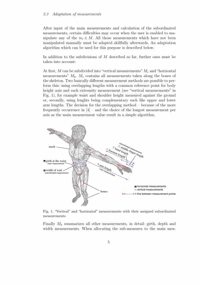
At first, M can be subdivided into“vertical measurements”Mv and“horizontalmeasurements” Mh. Mv contains all measurements taken along the bones ofthe skeleton. Two basically different measurement methods are possible to per-form this: using overlapping lengths with a common reference point for bodyheight axis and each extremity measurement (see “vertical measurements” inFig. 1), for example waist and shoulder height measured against the groundor, secondly, using lenghts being complementary such like upper and lowerarm lengths. The decision for the overlapping method – because of the morefrequently occurrence in [4] – and the choice of the longest measurement peraxis as the main measurement value result in a simple algorithm.

� �� �� �� �

� �� �� �� �� �

� �� �� �� �� �� �� �

����

mesh

��

horizontal measurements��vertical measurements

line between measurement points

forearm length

middle finger length

hand length

arm length

girth at the waist

width of wait

bones

main measurement

subordinated measurement

main measurement

subordinated measurements

Fig. 1. “Vertical” and “horizontal” measurements with their assigned subordinatedmeasurements

Finally Mh summarizes all other measurements, in detail: girth, depth andwidth measurements. When allocating the sub-measures to the main mea-

5

sures, it is important not to combine horizontal and vertical measures in oneequivalence class: ∀D(mi) : D(mi) ⊂ Mv ∨ D(mi) ⊂ Mh.

Further, the measures must be subdivided into fixed and modifiable ones bymeans of χ : M → {c,¬c}. All measures, where a value was allocated by theuser, are fixed. This normally includes all main measures.

One by one the equivalence classes D(mi), each of them represented by exactlyone mi ∈ Mm, 1 ≤ i ≤ #Mm, are changed according to the properties of theirelements.

3.3.1 Horizontal measurements

If D(mi) ⊂ Mh, then four cases have to be differentiated:

(1) ∀ mj ∈ D(mi) \ {mi} : χ(mj) = ¬c.The values of all modifiable subordinated measurements in D(mi) can becalculated from mi using equation (1).

(2) χ(mi) = ¬c ∧ ∃ m1, . . . , mk ∈ D(mi) \ {mi} : χ(m1) = . . . = χ(mk) = c.In this case the value of mi can be calculated as an average ofthe k fixed sub-measurements, for example as the geometric mean:

w(mi) = k

√

∏kj=1

w(mk)aij

. The values of the modifiable sub-measurements

in D(mi) can be found using equation (1).(3) χ(mi) = c ∧ ∃! mj ∈ D(mi) \ {mi} : χ(mj) = c.

If the input value of mj is larger than the the supposed value aij · w(mi),the values of the other subordinated measurements, especially if perpen-dicular to mj , must be reduced. If contrariwise w(mj) is smaller thanaij · w(mi), the other values have to be extended.The reason is, that inthis way an approximately elliptical shape of girth is preserved.

This correction can be implemented by multiplication with∆aij =

aij ·w(mi)

w(mj). The influence of ∆aij is proportionally dependant on the

smallest angle α between the measurement lines of fixed and modifiablemeasurements:

∀mk ∈ D(mi) \ {mi, mj} :

w(mk) = aik · (sin2 α · ∆aij + cos2 α) · w(mi).

(3)

α must be determined in advance, e.g. by means of a table containingthe angle sums of all subordinated measurements per class. The case ofmore than one subordinated fixed measurement should be forbidden dueto consistency matters, as illustrated in 4.2.4.

6

3.3.2 Vertical measurements

For D(mi) ⊂ Mv we propose the following procedure.

If χ(mi) = ¬c, then mi must be set fixed first: If ∀ mj ∈ D(mi) \ mi : χ(mj) = ¬c,this can easily be done, otherwise a more precise value for mi should be cal-culated from the value of the longest fixed subordinated measurement mk:w(mi) = w(mk)

aik. This ensures the exclusion of inconsistencies like w(mi) < w(mj)

for mj ∈ D(mi).

The class D(mi), containing n measurements, has to be augmented by anelement mn+1/i with χ(mn+1/i) := c and ai(n+1) := 0. Thereupon the elementsmj/i in the resulting set D(mi) ∪ {mn+1/i} must be indexed in a way that theircoefficients aij are in descending order (aik < aij for 1 ≤ j < k ≤ n + 1), i.e.the differences of the coefficients of successive measurements are defined by

∆aij := aij − ai(j+1) ≥ 0. (4)

m1/i = mi per pre-condition. Therefore m1/i is fixed. According to equation(1) aii = 1. Because mn+1/i is also fixed, every modifiable measurement mj isembedded within at least two fixed measurements: 1 ≤ k < j < l ≤ n + 1 forfixed measurements mk/i, ml/i. Hence its value can be calculated as follows:

The differences of the values of successive measurements ∆wj/i := w(mj/i) − w(mj+1/i)correspond to the differences of the closest surrounding fixed measurementsw(mk/i) − w(ml/i) like the associated differences of their coefficients:

∆wj/i

w(mk/i) − w(ml/i)=

∆aij

aik − ail

. (5)

For a detailled derivation of this equation see App. A. After calculation of all∆wj/i with equation (5) the value of a modifiable subordinated measurementis given by

w(mj/i) = w(ml/i) +l−1∑

z=j

∆wz/i (6)

The algorithm above only succeeds if the provided order conditions are metby the input values. Therefore it is reasonable to allow user data input only,if it fulfills a certain set of rules, e.g.

{body height > shoulder height, chest width ≤1

2· chest girth, . . .}.

7

4 Computation of the figurine

The measurement values, entered or calculated as shown in Section 3, must betransfered to the base model of a 3D figurine in such a way that distance andgirth values, determined from the skeleton and certain points of the model (inthe following: vertices, tripel consisting of x, y and z coordinates), will coincidewith the corresponding measurement data, while the figurine as such remainsrecognisable. That means the vertices outside of specifically manipulated pointareas (those coupled to a measurement) must be adapted with respect to theircoordinates in a way that a natural shaping of the figurine is preserved.

4.1 Vertical measurements

The transfer of all measurements mvj in Mv to the virtual figurine is a rathersimple task, because it is supported by the construction of the 3D model:the vertices are located at positions relative to certain virtual bones si takenfrom the skeleton S (see 4.2.1). Any modification of the bone length willproportionately affect those vertices attached to the bone: limb measurementsof the figurine are compressed or extended, without degrading the naturalnessof the shape – to a certain extent, of course.

To proceed, merely a map has to be built that allocates a length measurementto each bone si. The measurement is composed of multiples of differences takenfrom the available measurement values w(mvj). For example, the virtual thighbone is defined as

(crotch height − knee height) + 0.7 · (iliac bone height − crotch height).

Equation (7) enables to calculate the bone length in general:

len : S → R, len(si) =∑

j<k

asjk (w(mvk) − w(mvj)) , (7)

where mvj ∈ Mv ∪ {mv0}, w(mv0) = 0, 1 ≤ j, k ≤ #Mv. It is sufficientto define only a few asjk ∈ R in advance, for example by adjustment of mea-surement points on the real person and the start coordinates of bones in thefigurine, and setting all other asjk to zero.

8

4.2 Horizontal measurements

The adaptation of the figurine to horizontal measurements requires much moreeffort. The proposed procedure described below deals with at least two modelvariants of the same figurine which should differ as much as possible regardingmeasurement values, e.g. a thick and a thin base model. Between those thecomputed model will be located. This method reduces the input range for themhi in Mh, but as intended it protects against degenerated results.

4.2.1 Definitions

First of all, the structure of the figurine and auxiliary constructions used forthe adaptation procedure must be considered:

A figurine consists of an anchor point which defines its position in space,a skeleton S as well as a base mesh and in addition, one or more so-calledmorph meshes. The skeleton S represents a tree structure of single bonessi. Every si is defined by a reference to its parent bone (for the bones ofthe first hierarchy level: the anchor point) and a direction vector vr(si) with|vr(si)| = len(si). By means of traversing the tree the start and end coordinatesstart(si), end(si) ∈ R

3 can be calculated.

4.2.1.1 Meshes A mesh is assumed to be a sequence of vertices V =(v1, . . . , vn) which occur as triples, forming triangles in space, describing thesurface of the figurine, whereas the belonging of a vertex to a certain trianglegroup is irrelevant for the adaptation procedure.

The base mesh Vg consists of weighted vertices; that means for each vertexthe function coeffv : S → R maps coefficients to one or more bones thatindicate how the vertex will be moved if the position of the bone changes.The coefficients represent spheres of influence around bones which are alreadydefined during the building of one of the base models and are actually forseenfor the natural appearance of animations [1, 8]. Usage of these coefficients ismade in body areas (see below).

A morph mesh Vm = (v′

1, . . . , v′

n) represents a modified body shape derivedfrom the base mesh, for instance a thin or corpulent shape. Essentially Vm

corresponds to Vg, with the exception that the v′

i in comparision to the vi mayhave deviating coordinates, due to the modified shape. The weightings are thesame as in Vg. Thus, in particular Vg represents a morph mesh.

9

4.2.1.2 Planes As an auxiliary construction for mesh adaptation a setE of special planes ei is used. Each plane is located orthogonally to a boneand intersects with it at a height which corresponds to the height where themeasurement is taken on the real figurine (Fig. 2).

vr (bone(e))

origin(e)

start(bone(e))

coverage area near(e){

plane e

Fig. 2. Construction of a plane

Every measurement from Mh, if it is to be used, must be allocated to aplane. The characterisation of ei (see Fig. 2) comprises a bone, defined bybone(ei) ∈ S, an intersection value 0 ≤ cut(ei) ≤ 1, which identifies the pointof intersection relative to vr(bone(ei)), and Mei

⊂ Mh. To preserve consistancy(see 4.2.4), Mei is allowed to contain either a girth measurement, additionallya width or depth measurement or only two length values. Accordingly, E canbe divided into Eu, Eul and El.

Furthermore, there exists a value near(ei) and an orthonormal basis changematrix: basis(ei) ∈ M3(R). The former describes a coverage area, the latterserves to convert standard basis coordinates of a vertex into the coordinatesof a plane basis Bei

, which is constructed from the normalized vr(bone(ei))and two vectors in the plane, with their origins lying in the intersection withbone(ei), defined by

origin(ei) := start(bone(ei)) + cut(ei) · vr(bone(ei)). (8)

Thus the standard coordinates of a vertex can be converted into coordinatesof the plane by using the mapping

kei: V → V, v 7→ basis(ei) · (v − origin(ei)) (9)

Conveniently, the first coordinate (kei(v))1 always specifies the distance to ei,

and if (kei(v))1 is set to zero, a projection pi(v) onto the plane is gained.

Optionally, a so-called tag or orientation vector vT (ei) can be linked to ei. Itis necessary to find pairs of vertices, whose distances coincide with measured

10

width and depth values.

4.2.1.3 Body areas A body area bi is defined by one or several bonesSbi

⊂ S and one or two planes Ebi⊂ E . The set Vbi

of all vertices belongingto bi

3 is concluded through the equation

Vbi= {v ∈ Vg | ∃ si ∈ Sbi

: coeffv(si) 6= 0

andv lies between e1 and e2, if Ebi

= {e1, e2}

(ke1(v))1 > 0, if Ebi

= {e1}

.(10)

There are two aspects that lead to the second condition in equation (10):

(1) Body areas with a single plane are only intended for outer areas of limbs.(2) According to construction, directional vectors of planes always point out-

wards.

Whether v is positioned between two planes is either given by v lying on e1

or e2, that means pj(v) = v ⇐⇒ (kej(v))1 = 0, j ∈ {1, 2}, or can be derived

from the angle α of the perpendiculars λv1 6= 0 and λv2 6= 0 of v onto theplanes:

λvj = basis−1(ej) ·(

(kej(v))1, 0, 0

)

, j ∈ {1, 2} (11)

If α =λv1 · λv2

|λv1||λv2|is less than π

2, both planes are positioned on the “same side”

of v.

4.2.2 Convex hulls

As a first step it is necessary to define for each plane a corresponding setVg/near(ei) ⊂ Vg consisting of nearby vertices:

Vg/near(ei) = {v ∈ Vg : |(kei(v))1| ≤ near(ei) ∧ coeffv(bone(ei)) 6= 0}. (12)

A convex hull Vg/i of projections pi(v) of v ∈ Vg/near(ei) onto ei regarding Bi (see4.2.1.2) yields values for girth, depth and width measurements of the virtualfigurine in height of the plane. To be as precise as possible the value of near(ei)must be high enough not to allow #Vg/i to get too small, and low enough to

3 As an alternative to the division of Vg according to vertex weightings, Vbican

also be defined as a union of several submeshes, i.e. subdivisions of Vg carried outbeforehand.

11

guarantee that vertices far away from ei do not contort the shape. The higherthe vertex density of the base mesh, the lower near(ei) can be chosen.

The order of the elements in a convex hull, if constructed with standard al-gorithms, is immediately used for the calculation of the hull’s girth as sum ofthe differences of sequential elements:

girth(Vg/i) := v1 − v#Vg/i+

#Vg/i∑

k=1

(vk+1 − vk) (13)

Furthermore a tag vT (ei), used as a transposition from the origin of the plane,defines a zero mark for the angle. With vT (ei) vertices vb1, vb2, vt1, vt2 from Vg/i

can be found, whose absolute values of their differences |vb1 − vb2|, |vt1 − vt2|each correspond to a width or depth measurement.

Let the angles of the tag vT (ei) to the measurement lines of length measure-ments be pre-set in every plane ei containing lengths, e.g. 0 for widths, π

2for

depths, then vb1 and vb2 can be identified as those vertices opposing the ori-gin of the plane, whose connecting line, projected onto ei, forms the smallestpossible angle to vT (ei):

∀w ∈ Vg/i :vb1 · vT (ei)

|vb1||vT (ei)|≤

w · vT (ei)

|w||vT (ei)|∧

vb2 · vT (ei)

|vb2||vT (ei)|≥

w · vT (ei)

|w||vT (ei)|. (14)

vt1 and vt2 can be acquired accordingly.

4.2.3 Mesh selection

Thus in each of the different meshes all measurements of the virtual figurinethat coincide to the measurements mh ∈ Mh can be calculated. To create anew mesh, where the values for the horizontal measurements correspond tothose in Mh, an approach would be to detect for each body area bk thosetwo meshes Vm and Vm, which enclose Mh the most. For mhi ∈ Mei

, ei ∈ Ebk

only the following two equations must be fulfilled, whereas w, w and w′ arevalue mappings belonging to Vm, Vm respectively to a further mesh Vm′ andmhj ∈ Mej

, ej ∈ Ebk.

w(mhi) ≤ w(mhi) ≤ w(mhi) (15)

∀ Vm′ : w(mhi) ≤ w′(mhi) ≤ w(mhi) ∃ mhj : w(mhj) < w′(mhj)

and ∀ Vm′ : w(mhi) ≤ w′(mhi) ≤ w(mhi) ∃ mhj : w′(mhj) < w(mhj)(16)

12

Thereby the necessary changes of body shapes will be kept as small as possible.Unfortunately until now this approach fails due to the problematic realisationof smooth transitions between adjacent body areas. Nevertheless it can beused reasonably, if the measurements are not considered plane by plane butalltogether, therefore mhi ∈ Mh instead of mhi ∈ Mei

.

4.2.4 New convex hulls

Now each plane ei causes hulls Vm/i and Vm/i in Vm and Vm respectively. Basedon them a new hull Vm/i with the following characteristics is ascertainable:

•∀v ∈ Vm/i : v = v + rv · (v − v)

v ∈ Vm/i, v ∈ Vm/i, rv ∈ R, 0 ≤ rv ≤ 1(17)

Of course, v, v and v must coincide in their indices, determined during meshconstruction.

• All values for mhi ∈ Mei, calculated with Vm/i, match those w(mhi) deter-

mined in Section 3.

Hence – as considered before – the measurement data have to be checkedagainst those conditions 4 already during input. The next section deals withthat topic in detail.

If ei is in the equivalence class Eu, it is sufficient to determine one r for allv ∈ Vm/i by adapting the only measurement mu in Mei

, the girth of Vm/i,to the input w(mu). As a side-effect a single coefficient provides an optimalinterpolation of Vm/i and Vm/i. The adaptation of girth(Vm/i) occurs, startingwith r = 0, due to repeated changes of r and the subsequent determinationof girth(Vm/i). The value of r is increased as long as girth(Vm/i) < w(mu),and vice versa. Per successive decrease of the distance of steps w(mu) can beapproached to an arbitrary distance. In consequence of data verifications (see4.2.5) girth(Vm/i) and girth(Vm/i) cannot be exceeded. Thus – according toequation (17) – r remains between 0 and 1.

If ei ∈ El and ml ∈ Meiis a width measurement, a common coefficent r can be

stated directly. Are vb1, vb2 ∈ Vm/i, v′

b1, v′

b2 ∈ Vm/i, determined as describedin 4.2.2, then |v′

b2 − v′

b1| ≥ d := |vb2 − vb1| and ∆d = 12(w(ml) − d), so that

r =1

2

(

∆d

|v′

b1 − vb1|+

∆d

|v′

b2 − vb2|

)

=1

4

(

w(ml) − d

|v′

b1 − vb1|+

w(ml) − d

|v′

b2 − vb2|

)

(18)

4 One could allow r < 0 or r > 1, but this would result in a strong deviation ofthe figurine and in collisions of body areas, even if the interval [0, 1] is only slightlyexceeded.

13

The equation is illustrated by Fig. 3. The procedure for depth measurementsis the same.

Fig. 3. Minimal, maximal and desired lengths in relation

If ei belongs to Eul, i.e. Mei= {mu, ml} with girth and length measurements

mu and ml, there are already two values rl, ru required, with which the coef-ficient for every vertex v ∈ Vm/i is calculated individually via

rv = rl + ru · sin α, rl, ru ∈ R, 0 ≤ (rl + ru) ≤ 1, α =kei

(v) · d

|kei(v)||d|

, (19)

whereas d = vb2 − vb1, if a width measurement is present (see above), andd = vt2 − vt1, if ml is a depth measurement.

The equation can be explained as follows: first, like in the case of ej ∈ El,the convex hull Vm/i is increased to the desired size w(ml) and thus rl isdetermined. Then the points v of this hull are moved according to the angle ofkei

(v) and d until girth(Vm/i) is in the pre-set neighbourhood of w(mu). Theprocedure is akin to the girth approximation for planes in Eu, but the pointshave to be moved maximally if they are orthogonal to d and only little if thepoints are close to d, to preserve the correspondence to w(ml).

One could imagine the case of a plane ek with two length measurements inMek

, which is not dealt with seperatly because of the little gain of informationin comparison to Eul, but could be described as a combination of both casesmentioned above.

Furthermore it is noticable that more than two measurements per plane ei

will lead to inconsistencies (girth and width are predetermining the depth), ifthe shape between Vm/i and Vm/i is kept. A conversion of three measurementsinto the convex hull would not only require more complex methods, but wouldalso mean to loose the advantage of shape keeping for many combinations ofvalues.

14

4.2.5 Verification of user input

In most cases the verification of the input values is done by comparing themto the minimal and maximal girths and lengths of the convex hulls, whichwere calculated beforehand taking all morph meshes into account. For mea-surements assigned to planes in Eul this is not always sufficient: If both thegirth as well as a length in the same plane were set fixed, nevertheless some rv

may exceed the interval [0, 1], because, for preserving girth and width or depthrespectively, deviation of the ideal form, given by the meshes, is necessary (seeFig. 4).

minimal length

pre-set length

greatest possible length

greatest possible girth

smallest possible girth

minimal girth if length is pre-set

maximal girth if length is pre-set

Fig. 4. Limitation of the input area for the girth while length is fixed

To guarantee 0 ≤ r ≤ 1, first it has to be verified, whether the input lengthw(ml) does not fall below the minimal or exceed the maximal length, there-upon calculated rl and tested, whether the input girth lies between two newvalues for the minimal and maximal girth, girthl

min(ei) and girthlmax(ei), de-

pending on rl. The corresponding convex hulls are depicted as ellipses in Fig. 4.The values rv required for their calculation be means of equation (17) with α

as defined in equation (19), arise from the diagram:

girthlmin(ei) : rv = rl − rl · sin α

girthlmax(ei) : rv = rl + (1 − rl) · sin α.

(20)

Usage of equation (13) onto these hulls finally yields the new girth boundaries.

15

4.2.6 An adapted mesh

The construction of a mesh with a natural form, which is adjusted to allhorizontal measurements, is realised with the help of the body areas: Everyvertex v ∈ Vm lies in one, or at most two body areas (see 4.2.1.3). The latter is arare special case, because v ∈ Vbi

∩Vbj, i 6= j ⇐⇒ v = pk(v) ∧ ek ∈ Ebi

∩Ebj.

Therefore the consideration of only one area bv is enough.

The position of v is moved to the position of v′ ∈ Vm according to equation(17). Here rv is a combination of rv1 and rv2, the coefficients of the projectionspj(v) of v onto the up to two planes 5 e1 and e2 in Ebv under section 4.2.4. Soif e1 ∈ Eu ∪ El for example, r1v corresponds to r, the coefficient common toall point in the plane.

The closer v and ej , j ∈ {1, 2}, the stronger the influence of rjv on rv:

rv = (1 − q) · rv1 + q · rv2, q =|ke1

(v))1|

|ke1(v))1| + |ke2

(v))1|(21)

5 Improving recognizability

The transfer of a person’s body shape to a 3D model is not sufficient to ensurerecognizability. Regarding this the following important aspects have to beconsidered:

Up to this point the look of the skin, gender, age classes as well as the physiquein general and the characteristic of muscles or fat pads in particular werenot considered yet. The former can be realised using different skin textures.The other aspects demand extras like the construction of morph-mesh-groupsrepresenting combinations of additional user input data (e.g. male, middleaged, athletic) with a following update of the mesh-pool.

Nevertheless recognizability can be fulfilled only to a low degree if no emphasisis put on face modelling. There are approaches to transfer the shape and colourof a face, a person’s skin and eyes to a model that promise to meet the criteriaof a quick but equipment independent data input, as outlined in 3.1. Examplesare the construction of a 3D model of a head on the basis of a series of photostaken from different angles and the reshaping of a generic model throughiteration using a single photo.

For the procedure mentioned first UZR [12] is a viable solution (see also Section2). But good lighting, a non-reflecting background and manual post-editing of

5 If bv contains only one plane, set r2v = 0

16

the border between head and background for each of the at least ten photos arepreconditions for an acceptable quality. In addition a size adjustment of thehead for the export into the virtual model has to be performed. The lackingautomatisation of the data input operation is therefore the main disadvantageof this approach.

The second procedure, developed at the Max Planck institute for biologicalcybernetics, uses an average model of a head calculated from hundreds of 3Dscanned heads with variance values belonging to points in a 3D grid, as well asa front image and in order to get better results an additional profile photo ofthe head to be modelled. Modelling itself is done by bringing step by step colorvalues of the projection of the model into line with those in the photos, untilan energy value resulting from the variances reaches its minimum. A detaileddescription and promising results can be found in [2]. The main problem withthe practical use of this approach is the exclusion of hair.

The animation of the figurine and the possibility of dressing it are rathersupportive characteristics for recognition, but a substantial benefit in concreteapplications, as described in Section 1.

Using the popular technique of skeletal animation we were capable to supplythe figurine with multitudous animations. Information about changes of bonepositions (as described in 4.2.1) according to elapsed time is used to animateany vertex-object, in which the corresponding skeleton is integrated.

A realistic simulation of clothing, especially its behaviour under force effects,is a far more complex task. The mapping of colour and structure of clothingonto a figurine is no more than a first step: Only skin-tight clothes couldbe displayed convincingly. Natural movement of fabrics with knits and foldsrequire procedures like the particle system, whose concept is explained inApp. B, which is based on [10].

6 Conclusion

With the help of Fig. 5 the mesh, which was computed in a way as explainedabove, can be compared with the minimal and maximal mesh of the samefigurine. Those pictures show the possible variation of several measurements.Table 1 lists the corresponding measurement values. In the pictures the preser-vation of realistic body proportions can be recognised. Since for a represen-tation of the basic principles modelling of a few body areas is sufficient, atsome parts of the figurine little or no changes are evident. If the base mesheswere constructed with an appropriate expenditure, a significant increase of allranges could be achieved.

17

Fig. 5. minimal, adapted and maximized mesh

Table 1measurement values for Fig. 5

measurement (cm) minimal mesh adapted mesh maximal mesh

chest girth 98 110 119

thorax girth 90 102 115

waist girth 87 105 125

upper arm girth 35 43 50

wrist girth 19 22 31

thigh girth 51 61 70

Table 2 relates input measurement values to those values that are calculatedfrom a selection of the input values (marked bold). The deviation from thecalculated value to the input values can be traced back to the rigid calculationrules. It could be reduced, as mentioned in Section 5, by a subdivision intotypes like athletic, thickset etc. This could also include a different set of bonesfor each type, to enable the figurine to look even more realistic.

The computation time for the computation of an individualised figurine isabout a second on a gigahertz computer and a mesh of 10.000 vertices. But

18

Table 2Determinated data

measurement (cm) entered value calculated value

body height 182

waist height 107 109

knee height 52 49

chest girth 88

chest depth 22 20

arm length 76

forearm length 45 46

hand length 18 19

thigh girth 54

shank girth 36 35

since there have been done only a few attempts to optimize the procedureregarding the calculations or the reuseability of unchanged data, an almostrealtime behaviour seems to be achievable.

There is however no shortage of possible basic improvements for the describedprocedure. For example, due to the special demands on the meshs (same num-ber of vertices, Vg pre-sets the sequence of positions) up to now, the numberof available different meshes can only be increased manually and very slowly.A solution to this problem could be correspondence analysis, which meansthat from two morph meshes of nearly arbitrary descent each, vertex-couplesare determined automatically, e.g. by search for similar vertex coordinates orcolour values, and ordered according to Vg. Correspondence analysis wouldbe very helpful to extend the mesh pool more quickly and thus to increasesthe resemblance of the computed figurine to the real person. Just to mentionanother example: the raise of the number of measurements and planes usedfor adaption would probably have an effect of equal value.

However we deem the described procedure for modelling a figurine using bodymeasurement to be a promising start and well worth for further development.

A Derivation of equation (5)

The quotients of the fixed measurements mk/i, ml/i and mi are already de-

termined by user input. From the difference ∆pkl =w(mk/i)−w(ml/i)

w(mi)of these

19

quotients the ∆aij of the variable measurements in between can be recalcu-lated:

∆a∗

ij =∆pkl · ∆aij

aik − ail=

w(mk/i)−w(ml/i)

w(mi)· ∆aij

aik − ail(A.1)

The corresponding corrected value differences of these variable measurementsare derived from them by

∆wj/i = ∆a∗

ij · w(mi) =(w(mk/i) − w(ml/i)) · ∆aij

w(mi) · (aik − ail)· w(mi) (A.2)

=w(mk/i) − w(ml/i)

aik − ail· ∆aij .

This yields equation (5).

B Particle systems

Particle systems are based on the theory of cellular automata, where the stateof a particle at a certain timestep t + 1 is influenced by the states of itsneighbours at timestep t.

Thus to simulate textiles it is necessary to regard a woven piece of cloth asa two-dimensional set of particles, each of which is connected to its directneighbours. During the steps of calculation every particle tries to gain a moreideal position with respect to the positions of its neighbours.

To calculate the new position three parameters will be required: elasticity,shearing and bending forces. Elasticity defines the maxium offset of a particleto its neighbour. If this offset is exceeded, both particles try to move closertowards each other.

Shearing defines the angle between a particle and two of its adjacent particles.In case the angle exceeds a certain degree the neighbours will move towardseach other. Finally bending defines the allowed deviation of a particle from aline built up by two opposing neighbours. If the deviation becomes too large,the particle moves towards the centre of the line defined by the neighbours.

In order to achieve a realistic drape by this means, it is necessary to startwith an unbent piece of cloth, where all particles lie in one single plane andare affected by a force, e.g. gravity. As soon as an obstacle is hit while movingdownwards, for instance the body of a figurine, certain particles are no morecapable of moving and tensions with their neighbours arise.

20

Because in every step of calculation the three described parameters are in-cluded for the calculation of each particle of the cloth, tensions will be some-what counteracted. After a finite number of calculation steps a final statewill be reached, which accords with a real textile regarding appearance andarrangement of the folds.

A more detailed discussion regarding particle systems provides [10].

C Working group members

Nils Behrens, Bahir Bilgin, Sylvia Bluhm, Derya Bozkurt, Wilfried Grabbe,Christian Kluin, Alexander Kohn, Gerhard Kost, Siegfried Kramer, AlparslanKuzu, Magda Mazurek, Sebastian Meister, Cemal Oncel, Joachim Penk, ClaasPotthoff, Harry Rechten, Martin Spreckelmeyer, Vincent Stickdorn, MehmetUnal, Alexander Washausen, Florian Weiler, Tobias Wust

Acknowledgements

We wish to thank Jan Plath and Karl-Heinz Roediger for their support duringthis project.

References

[1] E. F. Anderson. Real-time character animation for computer games.Master’s thesis, National Centre for Computer Animation, BournemouthUniversity, 2001. URL http://ncca.bournemouth.ac.uk/newhome/

alumni/docs.[2] V. Blanz and T. Vetter. A morphable model for the synthesis of 3D faces.

In Siggraph 99 Conference Proceedings, New York, 1999. ACM.[3] Curious Labs, Inc. Poser 5. URL http://www.curiouslabs.com. Revis-

ited: Sept. 2003.[4] DIN – Deutsches Institut fur Normung e.V. DIN EN 979: Defini-

tionsgrundlagen menschlicher Korpermaße fur die Gestaltung technischer

Erzeugnisse. Beuth Verlag, Berlin, March 1993.[5] Discreet. 3ds max. URL http://www.discreet.com/products/3dsmax/.

Discreet is a subsidiary of Autodesk, Inc. Revisited: Sept. 2003.[6] B. Fluegel, H. Greil und K. Sommer. Anthropologischer Atlas. Grundlagen

und Daten. Alters- und Geschlechtsvariabilitat des Menschen. Wotzel,Frankfurt a.M., 1986.

21

[7] A. Fuhrmann, C. Groß, V. Luckas, and A. Weber. Interaction-free dress-ing of virtual humans. Computer & Graphics, 27:71–82, 2003.

[8] N. Lever. Real-time 3D Character Animation with Visual C++. FocalPress, Oxford, 2002.

[9] OptiTex Int. Runway. URL http://www.optitex.com/. Revisited:Oct. 2003.

[10] J. Plath. Realistic modelling of textiles using interacting particle systems.Computer & Graphics, 24:897–905, 2000.

[11] D. Thalmann. A new generation of synthetic actors: the real-time andinteractive perceptive actors. In Proceedings of the Pacific Graphics, pages200–219, 1996.

[12] UZR. 3D scanning with your digital camera. URL http://www.uzr.de.Revisited: Aug. 2003.

22