realistic application and air quality … application and air quality implications of distributed...
TRANSCRIPT
E n e r g y R e s e a r c h a n d D e v e l o p m e n t D i v i s i o n F I N A L P R O J E C T R E P O R T
REALISTIC APPLICATION AND AIR QUALITY IMPLICATIONS OF DISTRIBUTED GENERATION AND COMBINED HEAT & POWER IN CALIFORNIA
JUNE 2011 CEC-500-2015-032
Prepared for: California Energy Commission Prepared by: University of California Irvine Advanced Power & Energy Program

PREPARED BY: Primary Author(s):
Amin Akbari, Graduate Student Researcher Marc Carreras Sospedra, Post Doctoral Researcher Richard L. Hack, PE, CEM Vince McDonell, PhD Professor Scott Samuelsen, Director
221 Engineering Lab Facility Irvine, CA 92697-3550 CIEE Award # MAQ-07-01 CIEE Work Authorization # MR-026 Phone: 949-824-7302 | Fax: 949-824-7423 Contract Number: 500-02-004 Prepared for: California Energy Commission Marla Mueller Contract Manager Aleecia Gutierrez Office Manager Energy Generation Research Office Laurie ten Hope Deputy Director ENERGY RESEARCH AND DEVELOPMENT DIVISION Robert P. Oglesby Executive Director
DISCLAIMER This report was prepared as the result of work sponsored by the California Energy Commission. It does not necessarily represent the views of the Energy Commission, its employees or the State of California. The Energy Commission, the State of California, its employees, contractors and subcontractors make no warranty, express or implied, and assume no legal liability for the information in this report; nor does any party represent that the uses of this information will not infringe upon privately owned rights. This report has not been approved or disapproved by the California Energy Commission nor has the California Energy Commission passed upon the accuracy or adequacy of the information in this report.
ACKNOWLEDGEMENTS
The project team from the University of California Irvine’s (UCI) Advanced Power and Energy Program (APEP) consisted of Vince McDonell, PhD and Richard L. Hack, PE, CEM. Jeff Wojciechowski provided the program finance and administration support. A number of undergraduate students within the UCI-APEP provided support in the processing and organization of the data. Steven Lee, IT system manager for UCI-APEP oversaw several Computer Science graduate students and their efforts to assemble the SQL data base.
The project members thank Nicole Davis for her CIEE program administration support for this program.
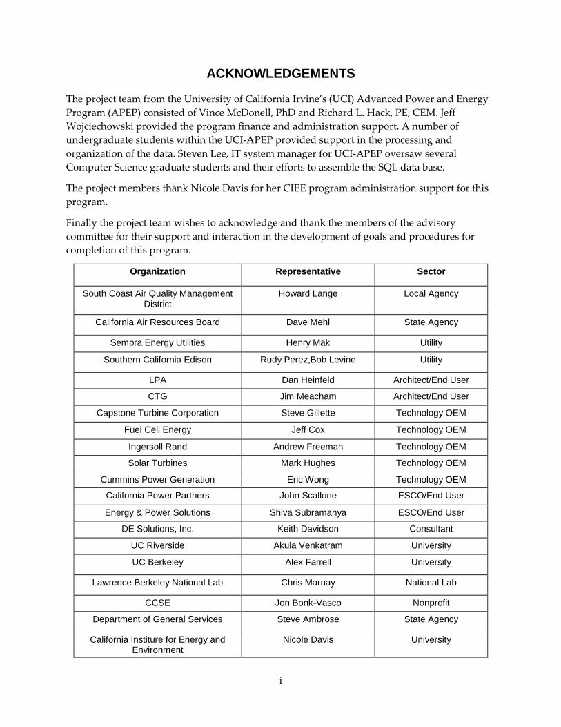
Finally the project team wishes to acknowledge and thank the members of the advisory committee for their support and interaction in the development of goals and procedures for completion of this program.
Organization Representative Sector
South Coast Air Quality Management District
Howard Lange Local Agency
California Air Resources Board Dave Mehl State Agency
Sempra Energy Utilities Henry Mak Utility
Southern California Edison Rudy Perez,Bob Levine Utility
LPA Dan Heinfeld Architect/End User
CTG Jim Meacham Architect/End User
Capstone Turbine Corporation Steve Gillette Technology OEM
Fuel Cell Energy Jeff Cox Technology OEM
Ingersoll Rand Andrew Freeman Technology OEM
Solar Turbines Mark Hughes Technology OEM
Cummins Power Generation Eric Wong Technology OEM
California Power Partners John Scallone ESCO/End User
Energy & Power Solutions Shiva Subramanya ESCO/End User
DE Solutions, Inc. Keith Davidson Consultant
UC Riverside Akula Venkatram University
UC Berkeley Alex Farrell University
Lawrence Berkeley National Lab Chris Marnay National Lab
CCSE Jon Bonk-Vasco Nonprofit
Department of General Services Steve Ambrose State Agency
California Institure for Energy and Environment
Nicole Davis University
i

PREFACE
The California Energy Commission’s Public Interest Energy Research (PIER) Program supports public interest energy research and development that will help improve the quality of life in California by bringing environmentally safe, affordable, and reliable energy services and products to the marketplace.
The PIER Program conducts public interest research, development, and demonstration (RD&D) projects to benefit California.
The PIER Program strives to conduct the most promising public interest energy research by partnering with RD&D entities, including individuals, businesses, utilities, and public or private research institutionsBuildings End-Use Energy Efficiency
• PIER funding efforts are focused on the following RD&D program areas:
• Buildings End-Use Energy Efficiency
• Energy Innovations Small Grants
• Energy-Related Environmental Research
• Energy Systems Integration
• Environmentally Preferred Advanced Generation
• Industrial/Agricultural/Water End-Use Energy Efficiency
• Renewable Energy Technologies
• Transportation
Realistic Application and Air Quality Implications of DG and CHP in California is the final report for the Realistic Application and Air Quality Implications of DG and CHP in California project (500-02-004). The information from this project contributes to PIER’s Energy-Related Environmental Research Program.
For more information about the PIER Program, please visit the Energy Commission’s website at www.energy.ca.gov/research/ or contact the Energy Commission at 916-654-4878
ii

ABSTRACT
The value and opportunity for distributed generation and the recovery of waste heat using combined heat and power for other beneficial purposes is increasing. Pressure on the existing electric distribution grid to meet increasing demands, and the needs to reduce emissions of both criteria pollutants and greenhouse gases, improve on site power reliability and reduce energy expenditures support local power generation systems located at the point of application. This study identified a variety of high energy use facilities in six sectors that would most likely benefit from distributed generation and combined heating and cooling, monitored and documented the typical energy profiles of the facilities, and assessed the effects, if any, of localized emissions from this technology on the immediate surroundings.
The study concluded that these facilities, based on their energy use profiles, could benefit from distributed generation and combined heat and power and including a significant impact on reducing energy demand. The study also found that using this technology reduces regional or pockets emission concentrations than the surrounding areas.
Please use the following citation for this report:
Akbari,Amin; Carreras Sospedra, Marc; Hack, Richard L.; McDonell, Vince; Samuelsen, Scott.. University of California at Irvine 2011. . Realistic Application and Air Quality Implications of DG and CHP in California. California Energy Commission. Publication number: CEC-500-2015-032.
iii

TABLE OF CONTENTS
Acknowledgements ................................................................................................................................... i
PREFACE ................................................................................................................................................... ii
ABSTRACT .............................................................................................................................................. iii
TABLE OF CONTENTS ......................................................................................................................... iv
LIST OF FIGURES .................................................................................................................................. vi
LIST OF TABLES ..................................................................................................................................... ix
EXECUTIVE SUMMARY ........................................................................................................................ 1
Introduction ........................................................................................................................................ 1
Project Purpose ................................................................................................................................... 1
Project Process .................................................................................................................................... 2
Project Results ..................................................................................................................................... 2
Project Benefits ................................................................................................................................... 3
CHAPTER 1: Introduction ...................................................................................................................... 5
1.1 Scientific and Technological Baseline ...................................................................................... 5
CHAPTER 2: Facility Identification ...................................................................................................... 7
2.1 Sector Identification Evaluation ............................................................................................... 7
2.1.1 Energy Information Resources / Sector Identification .................................................. 7
2.1.2 Sector Evaluation................................................................................................................ 8
2.1.3 Site Evaluation .................................................................................................................. 14
2.1.4 Sites Monitored ................................................................................................................. 15
CHAPTER 3: Thermal and Electric Demand Measurements ........................................................ 18
3.1 Utility and EMS Data ............................................................................................................... 19
3.2 Equipment Installation ............................................................................................................ 21
3.2.1 Electric Energy ......................................................................................................................... 21
3.2.2 Water Flow / BTU Meters ............................................................................................... 22
3.2.3 Gas Flow ............................................................................................................................ 23
3.2.4 Data Logging .................................................................................................................... 24
iv

CHAPTER 4: Data Base Generation ................................................................................................... 26
4.1 Data Base Architecture ............................................................................................................ 26
4.2 Fields .......................................................................................................................................... 26
4.2.1 Site Reporting Fields ........................................................................................................ 27
4.2.2 Site Characteristics Template ......................................................................................... 29
4.2.3 SQL Data Base Hosting and Use .................................................................................... 32
4.3 Preliminary Review and Comparison of Energy Profiles .................................................. 36
4.3.1 Commercial Office ........................................................................................................... 36
4.3.2 Grocery Store .................................................................................................................... 37
CHAPTER 5: Comparison of DG/CHP Utilization.......................................................................... 40
5.1 Sites Identified .......................................................................................................................... 40
5.1.1 SCAQMD DG/CHP .......................................................................................................... 40
5.1.2 CSUN ................................................................................................................................. 42
5.1.3 PCC .................................................................................................................................... 43
5.1.4 UCDMC ............................................................................................................................. 44
5.2 DG Operational Monitoring ................................................................................................... 44
5.3 Utilization Results .................................................................................................................... 45
5.3.1 AQMD ............................................................................................................................... 45
5.3.2 CSUN ................................................................................................................................. 51
5.3.3 PCC .................................................................................................................................... 61
5.3.4 UCDMC ............................................................................................................................. 66
5.4 Observations Regarding DG/CHP Utilization ..................................................................... 72
CHAPTER 6: Relative Exposure Analysis ......................................................................................... 74
6.1 Air Quality Impacts Modeling ............................................................................................... 74
6.1.1 Summary ........................................................................................................................... 74
6.1.2 Spatial Distribution of Distributed Generation for Retail Stores............................... 74
6.1.3 Energy Displacement Due to Combined Cooling Heating and Power .................... 78
6.1.4 Impact of DG/CHP Deployment on Regional Air Quality......................................... 88
v

6.1.5 Baseline Air Quality ......................................................................................................... 89
6.1.6 Air Quality Impacts of DG in Food/Grocery Stores .................................................... 91
6.1.7 Conclusions ....................................................................................................................... 93
6.2 Near Field Air Quality Impacts Modeling ........................................................................... 94
6.2.1 Modeling Conditions ....................................................................................................... 95
6.2.2 Domain and Grid Generation ......................................................................................... 95
6.2.3 Computational Approach ............................................................................................... 99
6.2.4 Result and Discussion.................................................................................................... 101
6.2.5 Conclusions ..................................................................................................................... 116
6.3 Near Field Population Analysis ........................................................................................... 117
6.3.1 GIS Field .......................................................................................................................... 118
6.3.2 Analysis ........................................................................................................................... 120
6.3.3 Population Impacts ........................................................................................................ 123
6.3.4 Summary ......................................................................................................................... 125
CHAPTER 7: Conclusions and Recommendations........................................................................ 127
REFERENCES ........................................................................................................................................ 140
LIST OF FIGURES
Figure 1: Site Characteristics Template: Page 1 ................................................................................... 30 Figure 2: Site Characteristics Template: Page 2 ................................................................................... 31 Figure 3: Site Characteristics Template: Page 3 ................................................................................... 32 Figure 4: SQL Data Base Location on Server ........................................................................................ 33 Figure 5: Connection to Server ............................................................................................................... 33 Figure 6: Alternate Connection Scheme ................................................................................................ 34 Figure 7: Sample Queries Using T-SQL ................................................................................................ 34 Figure 8: As Measured Typical Summer Energy Profile: Commercial Office Building ................ 36 Figure 9: Energy Profile After Application of DG/CHP: Commercial Office Building ................. 37 Figure 10: As Measured Typical Summer Energy Profile: Grocery Store ........................................ 39 Figure 11: Energy Profile After Application of DG.CHP: Grocery Store ......................................... 39 Figure 12: SCAQMD Four Microturbine Installation with Waste Heat Recovery (aka System 1)41 Figure 13: SCAQMD Three Microturbine Installation with Waste Heat Recovery (aka System 2) .................................................................................................................................................................... 41 Figure 14: CSUN 1 MW Molten Carbonate Fuel Installation ............................................................ 42 Figure 15: PCC MTG Array Installation (absorption chiller in foreground .................................... 43 Figure 16: UC Davis Medical Center Co-Gen Facility ........................................................................ 44
vi

Figure 17: AQMD MTG Installation: Typical Energy Profile: Oct-Dec 2008 ................................... 46 Figure 18: AQMD MTG Installation: Typical Overall Thermal Efficiency Profile: Oct – Dec 2008 .................................................................................................................................................................... 47 Figure 19: AQMD MTG Installation: Typical Energy Profile: Jan – March 2009 ............................ 48 Figure 20: AQMD MTG Installation: Typical Overall Thermal Efficiency Profile: Jan – Mar 2009 .................................................................................................................................................................... 49 Figure 21: AQMD MTG Installation; Typical Energy Profile; April - June 2009 ............................. 49 Figure 22: AQMD MTG Installation: Typical Overall Thermal Efficiency; April - June 2009....... 50 Figure 23: AQMD MTG Installation: Typical Energy Profile; July - Sept 2009 ............................... 50 Figure 24: AQMD MTG Installation; Typical Overall Thermal Efficiency; July - Sept 2009 ......... 51 Figure 25: CSUN Fuel Cell Installation; Typical Energy Profile; April – June 2008 ....................... 53 Figure 26: CSUN Fuel Cell Installation: Typical Fuel to Electric Power Efficiency; April – June 2008 ............................................................................................................................................................ 53 Figure 27: CSUN Fuel Cell Installation; Typical Overall Thermal Efficiency; April – June 2008 . 54 Figure 28: CSUN Fuel Cell Installation; Typical Energy Profile; July - Sept 2008 .......................... 54 Figure 29: CSUN Fuel Cell Installation: Typical Fuel to Electric Power Efficiency; April – June 2008 ............................................................................................................................................................ 55 Figure 30: CSUN Fuel Cell Installation; Typical Overall Thermal Efficiency; July - Sept 2008 .... 55 Figure 31: CSUN Fuel Cell Installation; Typical Energy Profile; Oct – Dec 2008............................ 56 Figure 32: CSUN Fuel Cell Installation: Typical Fuel to Electric Power Efficiency; Oct – Dec 2008 .................................................................................................................................................................... 56 Figure 33: CSUN Fuel Cell Installation; Typical Overall Thermal Efficiency; Oct – Dec 2008 ..... 57 Figure 34: CSUN Fuel Cell Installation; Typical Energy Profile; Jan – March 2009 ....................... 57 Figure 35: CSUN Fuel Cell Installation; Typical Fuel to Electric Power Efficiency; Jan – March 2009 ............................................................................................................................................................ 58 Figure 36: CSUN Fuel Cell Installation; Typical Energy Profile; April – June 2009 ....................... 58 Figure 37: CSUN Fuel Cell Installation; Typical Fuel to Electric Power Efficiency; April – June 2009 ............................................................................................................................................................ 59 Figure 38: CSUN Fuel Cell Installation; Typical Energy Profile; July – Sept 2009 .......................... 59 Figure 39: CSUN Fuel Cell Installation; Typical Fuel to Electric Power Efficiency; July – Sept 2009 ............................................................................................................................................................ 60 Figure 40: CSUN Fuel Cell Installation; Typical Energy Profile; Oct – Dec 2009............................ 60 Figure 41: CSUN Fuel Cell Installation; Typical Fuel to Electric Power Efficiency; Oct – Dec 2009 .................................................................................................................................................................... 61 Figure 42: PCC MTG / Chiller Array; Typical Electric Energy Output; Sept-Dec 2008 ................. 62 Figure 43: PCC MTG / Chiller Array; Typical Overall System Efficiency; Sept – Dec 2008 .......... 62 Figure 44: PCC MTG / Chiller Array; Typical Electric Energy Output; Jan – Mar 2009 ................ 63 Figure 45: PCC MTG / Chiller Array; Typical Overall System Efficiency; Jan-Mar 2009 .............. 63 Figure 46: PCC MTG / Chiller Array; Typical Electric Energy Output; Apr-Jun 2009 ................... 64 Figure 47: PCC MTG / Chiller Array; Typical Overall System Efficiency; Apr-Jun 2009 .............. 64 Figure 48: PCC MTG / Chiller Array; Typical Electric Energy Output; Jul-Sept 2009 ................... 65 Figure 49: PCC MTG / Chiller Array; Typical Overall System Efficiency; Jul-Sept 2009 .............. 65 Figure 50: PCC MTG / Chiller Array; Typical Electric Energy Output; Oct-Nov 2009 .................. 66
vii

Figure 51: PCC MTG / Chiller Array; Typical Overall System Efficiency; Oct-Nov 2009 ............. 66 Figure 52: UCDMC Overall Electric Generation Efficiency; Oct - Dec 2008 .................................... 68 Figure 53: UCDMC: Overall Thermal Efficiency; Oct -Dec 2008 ....................................................... 68 Figure 54: UCDMC: Overall Electric Generation Efficiency; Jan - Mar 2009 ................................... 69 Figure 55: UCDMC Overall Thermal Efficiency; Jan - Mar 2009 ....................................................... 69 Figure 56: UCDMC Overall Electric Generation Efficiency; April - Jun 2009 ................................. 70 Figure 57: UCDMC Overall Thermal Efficiency; April - June 2009 .................................................. 70 Figure 58: UCDMC Overall Electric Generation Efficiency; July - Sept 2009 .................................. 71 Figure 59: UCDMC: Overall Thermal Efficiency; July - Sept 2009 .................................................... 71 Figure 60: GIS land use data of spatial distribution of retail centers in the South Coast Air Basin .................................................................................................................................................................... 76 Figure 61: Insert of Figure 60 Showing GIS Land Use Data of Spatial Distribution of Retail Centers in and Around the Newport Beach Area ............................................................................... 77 Figure 62: Options for Spatial Distribution of DG/CHP Systems for Food Retail Stores: ............. 78 Figure 63: Energy Balance in Food Retail Store; ICE Prime Mover; HVAC Priority ..................... 84 Figure 64: Energy Balance in Food Retail Store; ICE Prime Mover; HVAC Priority ..................... 85 Figure 65: Energy Balance in Food Retail Store. MCFC Prime Mover, HVAC Priority ................ 86 Figure 66: Energy Balance in Food Retail Store. MCFC Prime Mover; High Temperature Refrigeration ............................................................................................................................................. 87 Figure 67: UCI-CIT Airshed Modeling Domain of the South Coast Air Basin of California ........ 90 Figure 68: Baseline Pollutant Concentrations Resulting from Summer Emissions for the Year 2005: ........................................................................................................................................................... 91 Figure 69: ICE DG/CHP Application in Food/Grocery: Changes in Pollutant Concentrations .... 93 Figure 70: MCFC DG/CHP Application in Food/Grocery: Changes in Pollutant Concentrations: .................................................................................................................................................................... 93 Figure 71: Domain for Analysis (not to scale) ...................................................................................... 98 Figure 72: Velocity 8.25ft Stack Height Vertical Exhaust ................................................................. 101 Figure 73: NOx Concentration for 8.25ft Stack Height Vertical Exhaust ....................................... 102 Figure 74: NOx Concentration; Y=5ft for 8.25ft Stack Height Vertical Exhaust ............................ 102 Figure 75: Velocity for 8.25ft Stack Height +45 Tilted ....................................................................... 102 Figure 76: NOx Concentration for 8.25ft Stack Height +45 Tilted ................................................... 103 Figure 77: NOx Concentration; Y=5ft for 8.25ft Stack Height +45 Tilted ....................................... 103 Figure 78: Velocity for 8.25ft Stack Height -45 Tilted ....................................................................... 103 Figure 79: NOx Concentration for 8.25ft Stack Height -45 Tilted ................................................... 104 Figure 80: NOx Concentration; Y=5ft for 8.25ft Stack Height -45 Tilted ........................................ 104 Figure 81: Velocity 8.25ft stack height vertical exhaust (5mph wind speed) ................................ 104 Figure 82: NOx Concentration for 8.25ft Stack Height (5mph wind speed) .................................. 105 Figure 83: NOx Concentration; Y=5ft for 8.25ft Stack Height (5mph wind speed) ...................... 105 Figure 84: Velocity for 15ft Stack Height vertical exhaust ............................................................... 105 Figure 85: NOx Concentration for 15ft Stack Height vertical exhaust ........................................... 106 Figure 86: NOx Concentration; Y=5ft for 15ft Stack Height .............................................................. 106 Figure 87: Vertical velocity for 15ft Stack Height +45 tilted ............................................................. 106 Figure 88: NOx Concentration for 15ft Stack Height +45 tilted ....................................................... 107
viii

Figure 89: NOx Concentration; Y=5ft for 15 ft Stack Height +45 tilted ........................................... 107 Figure 90: Velocity for 15ft stack height -45 tilted ............................................................................. 107 Figure 91: Velocity for 15ft stack height -45 tilted ............................................................................. 108 Figure 92: NOx Concentration for 15ft Stack Height -45 tilted ........................................................ 108 Figure 93: Velocity for FW, 8.25ft stack height .................................................................................. 108 Figure 94: NOx Concentration for FW, 8.25ft stack height ............................................................... 109 Figure 95: NOx Concentration; Y=5ft for FW, 8.25ft stack height .................................................... 109 Figure 96: Velocity for HW, 8.25ft stack height ................................................................................. 109 Figure 97: NOx Concentration for HW, 8.25ft stack height .............................................................. 110 Figure 98: NOx Concentration; Y=5ft for HW, 8.25ft stack height ................................................... 110 Figure 99: Velocity for FW, 20ft stack height ..................................................................................... 110 Figure 100: NOx Concentration for FW, 20ft stack height ................................................................ 111 Figure 101: NOx Concentration; Y=5ft for FW, 20 ft stack height .................................................... 111 Figure 102: Velocity for HW, 20ft stack height .................................................................................. 111 Figure 103: NOx Concentration for HW, 20ft stack height ............................................................... 112 Figure 104: NOx Concentration; Y=5ft for HW, 20ft stack height .................................................... 112 Figure 105: Velocity for FW, 25ft stack height ................................................................................... 112 Figure 106: NOx Concentration for FW, 25ft stack height ................................................................ 113 Figure 107: NOx Concentration; Y=5ft for FW, 25ft stack height ..................................................... 113 Figure 108: Velocity for HW, 25ft stack height .................................................................................. 113 Figure 109: NOx Concentration for HW, 25ft stack height ............................................................... 114 Figure 110: NOx Concentration; Y=5ft for HW, 25ft stack height .................................................... 114 Figure 111: Velocity for FW, 30ft stack height ................................................................................... 114 Figure 112: NOx Concentration for FW, 30ft stack height ................................................................ 115 Figure 113: NOx Concentration; Y=5ft for FW, 30ft stack height ..................................................... 115 Figure 114: Velocity for HW, 30ft stack height .................................................................................. 115 Figure 115: NOx Concentration for HW, 30ft stack height ............................................................... 116 Figure 116: NOx Concentration; Y=5ft for HW, 30ft stack height .................................................... 116 Figure 117: Map of Analysis Area ....................................................................................................... 119 Figure 118: Example – Hotel Buildings for DG Siting ...................................................................... 120 Figure 119: Intersection of Residential and DG Buffer Zones ......................................................... 121 Figure 120: Residential Population and Possible DG/CHP Installations ....................................... 124
LIST OF TABLES Table 1: Market Potential for Traditional CHP in Existing Facilities in California .......................... 8 Table 2: Aggregate Technical Market Potential for Traditional CHP in Existing Facilitie .............. 9 Table 3: Top 10 Sectors for Evaluation based upon Current and Future DG/CHP potential in California ..................................................................................................................................................... 9 Table 5: Weighting Factors for Evaluation Criteria ............................................................................. 11 Table 6: Ranking of Sectors Inclusive of Annual Load Factor Consideration ................................. 13 Table 7: Final Sectors Chosen for Monitoring ...................................................................................... 14 Table 8: Site Evaluation Criteria ............................................................................................................. 14 Table 9: Sector Breakdown for Site Participation ................................................................................ 15 Table 10: Summary of Site Identification by Sector and Source of Energy Data ............................ 20
ix

Table 11: Comparison of Measurement Accuracy with ASERTTI Protocols................................... 25 Table 12: SQL Data Base Parameters ..................................................................................................... 35 Table 13: Electricity Consumption in Food Retail and Related Activities by County (from the energy consumption data management system, California Energy Commission ......................... 79 Table 14: Distribution of Electricity Needs by End Use in Food Retail Stores (ASHRAE, 2008) .. 80 Table 15: Parameters for the Electrical and Cooling Systems Considered in the Study ................ 82 Table 16: DG/CHP Application in Food Retail Stores in the South Coast Air Basin of California .................................................................................................................................................................... 83 Table 17: Emissions Factors for MCFC and ICE Installations ............................................................ 88 Table 18: Total Emissions from Deployment of CCHP Installations in Food Retail Stores .......... 89 Table 19: Net Changes in Emissions Due to Two CHP Scenarios, in Percentage (%) with Respect to Total Basin-Wide Emissions in the South Coast Basin of California in the Year 2005............... 92 Table 20: Plume Model Parameters: ...................................................................................................... 96 Table 21: Studied Cases ........................................................................................................................... 99 Table 22: Detailed Governing Equations ............................................................................................ 100 Table 23: Potential Residential Population Impact of DG ................................................................ 125
x

EXECUTIVE SUMMARY
Introduction California’s electricity demand is increasing, putting pressure on the existing electric transmission system to meet this demand, increase on site power reliability, and reduce criteria pollutants, greenhouse gases, and energy expenditures. In the right circumstances, distributed generation (DG) – small-scale power generation located close to electricity loads – can reduce or eliminate new generation, transmission, and distribution infrastructure. Distributed generation can improve the efficiency of the electric system by avoiding transmission and distribution losses that occur when electricity travels over power lines. These systems can also improve reliability by providing electricity to a site regardless of what might occur on the power grid.
Distributed generation that delivers electricity during peak demand periods can free up other generating capacity and ease transmission bottlenecks and line congestion. Distributed energy can also be installed to recover waste heat, using it for heating and/or cooling, referred to as combined heat and power (CHP).Project Purpose
Project Purpose Use of small and mid-sized DG/CHP in California is expected to grow significantly between now and 2020 directed by ongoing policy and legislation to help stabilize the state’s electricity supply and meeting greenhouse gas reduction goals. However, using DG /CHP in urban areas can potentially increase human exposure to air pollutants. Furthermore, the energy efficiency of the DG/CHP systems can vary widely depending on the technology used and how it operates. The available data of averaged profiles and predicted building load demands is not adequate to understand the performance of these units. This study identified facilities that would most likely benefit from DG/CHP, addressed the lack of validity with the current assumed load profiles defining actual building load profiles, and provided the data to accurately predict the DG/CHP’s impact on local energy use and air quality.
An emission signature estimate of the installed or “as deployed” DG/CHP device is necessary to accurately determine the air quality impacts of the DG/CHP. The emissions produced by a DG/CHP system depend on the technology used, how it is operated and its overall efficiency.
How the DG/CHP system operates is directly tied to the application being used, the electric and natural gas utility rates and the building demand profile. As a result, it is necessary to understand how a given DG/CHP system operates for various applications to establish a representative emissions signature.
For DG/CHP to be cost effective, and meet California Air Resources Board certification emission limits, the heat waste must be recovered almost all of the time. For most applications that consider DG/CHP, the monthly or yearly quantities of electricity and heat use indicate that a DG/CHP system should work efficiently. This, however, is usually not the case due to the miss- match between the moment-by-moment electric and heat demand. As a result, DG/CHP systems must match the timing of the required heat and electricity on a real-time basis, since storing either heat or electricity even on a short term basis is not economically practical. In
1

addition, the temperature of waste heat from the DG generator must meet minimum qualitylevels demanded by the load requirements. If either the timing or quality does not match, then only a small fraction of the waste heat can be used, greatly decreasing the overall efficiency of the DG/CHP unit and potentially increasing overall emissions from the unit.
Project Process Hospitals, hotels, jails/prisons, colleges/universities, large commercial office buildings, and food/grocery facilities were identified to monitor as most likely to benefit from installing DG/CHP and the most to impact the grid and environment. More than 200 sites were considered to participate in the program based on a combination of criteria with a total of 58 facilities participating in the program:
• Hospital/Health Care Facilities - 6
• Hotels - 4
• Jails/Prisons - 9
• Colleges/Universities - 9
• Large Commercial Offices - 18
• Food/Grocery Facilities - 12 (eleven grocery stores + one warehouse distribution center)
This energy monitoring effort documented the energy profile of the represented facilities including:
• Energy use including electricity grid or natural gas lines crossing the facilities property line,
• Any on-site power generation whether fuel based or renewable,
• The energy required for heating and cooling demands, whether domestic hot water or heating, ventilating and air conditioning, and
• The energy required for process heating and cooling, that could be met with waste heat recovery strategies.
For the majority of these sites the researchers obtained this energy data for at least 12 months (to represent seasonal variations) at intervals of 15 minutes.
Project Results Evaluating the energy profiles and the applicability of DG/CHP to the sites suggest that all six sectors can use the DG/CHP in an effective manner to increase overall facility efficiency, reduce criteria pollutant and greenhouse gas emissions, and likely provide initial economic benefits.
However, the actual implementation and savings may be different from theory. The researchers also monitored facilities that currently had operating DG/CHP systems installed. Of the 58 participating facilities, four had operational DG/CHP systems (one site had two installations) ranging from a total generating capacity of 195 kilowatts to 25 megawatts.
2

Actual operating DG/CHP systems show seasonal variations in waste heat captured that is reflective of the ambient temperature variations especially for smaller facilities and smaller systems. That is, for systems that use waste heat recovery exclusively for domestic hot water and space heating, the amount of heat recovery and hence the overall system efficiency varied with the hot water demands/recovery. Summer/warm month demands are lower when compared to the demands in winter/cool months and result in lower waste energy recovery and lower overall thermal efficiency. Conversely, one of the hospital sites used waste heat for multiple applications including space heating, hot water, steam, and to drive a 100 ton absorption chiller for cooling demands. The overall size and continued demand for space conditioning 24/7 in various forms results in annually higher overall efficiency with highest efficiency in the summer when the waste heat can be used for cooling.
Microturbine (smaller) generator DG/CHP systems comprised three of the monitored installations and demonstrated nominal annual overall thermal efficiencies of approximately 55 percent. The molten carbonate fuel cell installation exhibited nominal annual overall thermal efficiencies of approximately 70 percent and at times greater than 85 percent, partly owing to the combination of sensible and latent heat recovery. However, operational issues associated with the latter resulted in erratic and inconsistent waste heat recovery. For the large turbine co- generation facility, the operational on-time generating availability was greater than 97 percent and reflected the vital and highly integrated nature of the system to support the entire electric and thermal demands for the facility.
The results of the real world DG/CHP system monitoring also reflect different levels of system support that appears to be related to either the critical nature of the supplied energy, the cost of the system, or both. Generally the smaller systems (microturbine) while flexible do not represent significant financial benefit for the facility and are not highly valued. Their poor operational history performance and reduced efficiency are a result of general neglect due to low budget and maintenance support. In addition to higher efficiencies, large systems have maintenance and financial support and high on-line time generating power (or at least the ability to generate power if desired also known as “availability”).
Researchers also investigated the air quality impact of DG/CHP on the nearby surrounding population. Applying DG/CHP to all of the sectors in the South Coast Air Basin could, on average, affect two percent of the population through possible impacts on local air quality as defined by the 100 meter radius from the DG system.
Project Benefits This research supports California’s goal to encourage developing environmentally-sound DG/CHP projects by providing a better understanding of the efficiencies and emissions of various applications of DG/CHP systems to optimize system design and placement. This research will also help policymakers value DG/CHP to effectively determine the amount of emission credits to allocate DG/CHP units. For example, this research showed that the food and grocery industry including grocery and convenience stores which currently have few DG/CHP systems, would be an excellent candidate for this system while reaping one of the highest efficiencies and smallest emissions footprint. In California as a whole, there are more than 5,600
3

food/convenience stores considered “medium” or “large” and use approximately 5,100 GW-hr of energy consumption. The study indicates that a DG/CHP system could typically meet more than 90 percent of all of the energy demands at a food/grocery store with both the on-site electric power generation and displacing more than 50 percent of the refrigeration needs with a thermally activated cooling driven by waste heat. Further, the overall thermal efficiency of such a system would be greater than 75 percent and reducing natural gas consumption by approximately 20 percent. Saving 10.2 million MMbtu of natural gas would reduce 544,000 million tons of carbon dioxide emissions annually.
The study also concludes that technology advances in this arena will help the DG/ CHP industry provide better products to meet California’s electricity generation goals. Specifically, developing and improving thermally activated cooling systems to support the medium temperature refrigeration applications are crucial to the potential for DG/CHP to provide the noted energy efficiency opportunities.
4
CHAPTER 1: Introduction To accurately determine the air quality impacts of distributed generation (DG) sited in possible California locations, an estimate of the emission signature of the “as deployed” DG device is needed. For example, DG can be installed in a way that recovers the waste heat and uses it for heating and/or cooling, which is referred to as combined heat and power (CHP). The mass of emissions produced by a DG/CHP system depends on how it is operated and its overall efficiency and displaced emissions from the heating system. How the DG/CHP system operates is strongly tied to the application it is being used in, the electric and natural gas utility rates, and the building demand profile. As a result, it is necessary to understand how a given DG/CHP system is operated for various applications in order to establish a representative emissions signature.
For CHP to be cost effective, the waste heat must be recovered most if not all of the time. For most applications that consider CHP, the monthly or yearly quantities of electricity and heat use indicate that a CHP system should work efficiently. However, this is often not the case due to the miss-match between the moment-by-moment electric and heat demand. As a result, CHP systems need to match the timing of the needed heat and electricity on a real-time basis, since storing either heat or electricity even on a short term basis is not economically practical. In addition, the temperature of waste heat from the DG generator must meet minimum quality levels demanded by the load requirements. If either the timing or quality does not match, then only a small fraction of the waste heat can be used, greatly decreasing the overall efficiency of the CHP unit and increasing overall emissions. As a result, time resolved information regarding building load (electrical and thermal) demands and how DG/CHP systems are deployed to optimally meet this demand is needed to accurately determine the emissions profile of the system.
1.1 Scientific and Technological Baseline The temperature and timing demand for heat energy compared to electricity use is not established for a significant sample of commercial facilities located in California urban areas. Hourly electricity use profiles are available for some larger facilities such as hospitals. Limited highly resolved time base load profile data (e.g. 15-minute interval) is may be found for businesses and facilities with electrical demands of greater than 1 MW. But generally, building load information is commonly reported in annual or monthly averages, likely owing to cost for acquisition and deployment of the monitoring equipment.(EEA-2003)1 (Onsite SYCOm-1999)2
1EEA, National Account Sector Energy Profiles 2003
2 ONSITE SYCOM, Market Assessment of Combined Heat and Power Market in California, Energy Corporation, December 22, 1999
5
(Onsite-SYCOM-2000)3 (EEA-2005)4, Moreover, existing CHP applications of 1 MW and less are not regulated and relevant operational data are often not retained or reported. Some information regarding building energy consumption is available through the Energy Information Agency. An example is the Commercial Building Energy Consumption Survey from 1995 which summarizes information for 27 different general building types and provides a wealth of information as a function of various parameters such as year built and HVAC technology type. However, this information is all time averaged and generally tabulated on an annual basis. The U.S. Department of Energy has available annual Building Energy Databooks which again provide detailed tabulated data on energy consumption for different building types. Again, however, this information is based on annual consumption. As a result, a need exists for detailed hourly (or even further temporally resolved) information on typical building electricity and thermal usage to identify potential DG/CHP systems that might be deployed to meet those requirements. Additionally, this information can be used to more accurately assess the air quality impact and total energy requirements of DG/CHP system.
Another benefit of collecting detailed usage information is that building simulation efforts have evolved to the point where hourly demand data can be utilized. Examples of simulation software that can incorporate hourly building demand information includes Distributed Energy Resource Customer Adoption Model (DER-CAM) (Siddiqui, et al., 2003)5 and eQUEST(DOE)6 eQUEST incorporates the DOE-2 building simulation software, which has libraries of simulated building demand information. To support some of these modeling platforms, data have been obtained which is similar in nature to that collected in this effort. However, it is very sparse in nature, not systematic across many building types, and does not have the time resolution desired. Any of these existing data, to the extent possible, are included in the database developed as part of this effort so they can be included in the overall air quality impact assessment.
In summary, before this study very limited data was available with which to carry out accurate predictions of the air quality impacts and total energy consumption of DG/CHP systems in California. In this study, a systematic collection of this information was conducted with the time resolution necessary to (1) establish advanced DG deployment scenarios (e.g., based on real time price signals or “emission based deployment” strategies) and (2) facilitate the subsequent integration of this information into an interactive database that can be used in conjunction with air quality impact models to provide air quality impact estimates.
3 The Market and Technical Potential for Combined Heat and Power in the Commercial/Institutional Sector, ONSITE SYCOM Energy Corporation, January 2000
4 The Combined Heat and Power Database, EEA, 2005 http://www.eea-inc.com/testchp/index.html
5 Siddiqui, A., Firestone, R., Ghosh, S., Stadler, M., Edwards, J., and Marnay, C. (2003). Distributed Energy Resource Customer Adoption Modeling with Combined Heat and Power Applications.
6 DOE, Quick Energy Simulation Tool (available at http://www.doe2.com/equest/) accessed 10 January 2006.
6
CHAPTER 2: Facility Identification Intuitively, facilities that would most benefit from Distributed Generation (DG)/Combined Heat and Power (CHP) would be those that have high thermal loads or air conditioning loads that also have coincident needs for electric power. However, in reality a more complex methodology taking into account size of the sector (in terms of overall megawatts), financial feasibility of installation for the typical owner, need for grid-independent power or back-up power, and other factors, went into the evaluation of the sites. Applying DG/CHP and its potential impacts have been evaluated on several occasions with detailed reports defining “global” system requirements (such as system power needs, total potential installed capacity) across a variety of facility types (SIC code delineated facilities) have been published. With the compiled DG/CHP system application information, a review of actual DG/CHP deployment, and through a process of weighting the facility attributes listed above, this study provides a ranking of the applicability and benefit of DG/CHP for each of the SIC sectors. This was reviewed with the technical advisory committee (TAC) and a final set of “sectors” identified for the program. At the end of the study, six sectors were identified and data from approximately 60 sites compiled.
2.1 Sector Identification Evaluation 2.1.1 Energy Information Resources / Sector Identification Data from “Assessment of California CHP Market and Policy Options for Increased Penetration” (EEA-2005)7 , a report for the California Energy Commission, was used to screen and rank sectors based upon the current and projected cumulative energy production needs, the current and projected co-generation needs, and the size of the on-site energy needs (Table 1 and Table 2). This information was combined with the data bases documenting the self-generation application records for California (SCE-2006)8 and the California Commercial End Use Survey (ITRON 2006)9 Additional input from the TAC on sectors germane to the overall program goals was garnered. The result was a ranked list of ten possible sectors, all demonstrating energy intensity and CHP opportunity in California (Table 3) for further evaluation.
7 EEA, Assessment of California CHP Market and Policy Options for Increased Penetration, April 2005; prepared for the California Energy Commission by the Electric Power Research Institute (EPRI) and Energy and Environmental Associates (EEA); Report Number CEC-500-2005-060-D
8 SCE, California Self Generation Incentive Program Data Base: www.sce.com/RebatesandSavings/SelfGenerationIncentiveProgram
9 ITRON Inc.,California Commercial End Use Survey, March 2006; prepared for the California Energy Commission by Itron Inc, Report NumberCEC-400-2006-005
7
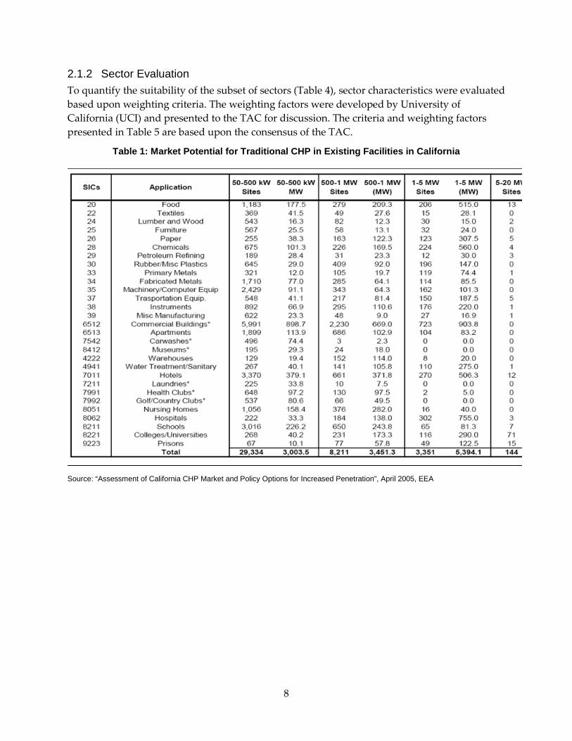
2.1.2 Sector Evaluation To quantify the suitability of the subset of sectors (Table 4), sector characteristics were evaluated based upon weighting criteria. The weighting factors were developed by University of California (UCI) and presented to the TAC for discussion. The criteria and weighting factors presented in Table 5 are based upon the consensus of the TAC.
Table 1: Market Potential for Traditional CHP in Existing Facilities in California
Source: “Assessment of California CHP Market and Policy Options for Increased Penetration”, April 2005, EEA
8
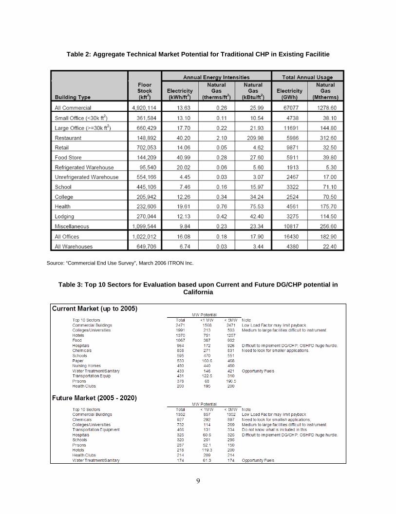
Table 2: Aggregate Technical Market Potential for Traditional CHP in Existing Facilitie
Source: “Commercial End Use Survey”, March 2006 ITRON Inc.
Table 3: Top 10 Sectors for Evaluation based upon Current and Future DG/CHP potential in California
9

Table 4: Criteria for Evaluation of Sectors
Sector Analysis Current Market Potential - weighting based upon installed MW and CHP application
Future Market Potential – weighting based upon installed MW potential CHP application
Utilization of Opportunity Fuels – added weighting if renewable fuels can be incorporated Site Cooperation/Regulatory Hindrances – weighting to consider:
Are sites supportive of DG/CHP in general?
Are there government or other regulatory agencies that are reluctant to support DG/CHP or have substantial hurdles that can complicate and extend the process to the point of being undesirable. For example
• OSHPD for hospitals and health care • State Architect for public institutions
CHP Integration Potential/Value – weighting based upon potential for efficiency and economic benefits to end user.
10
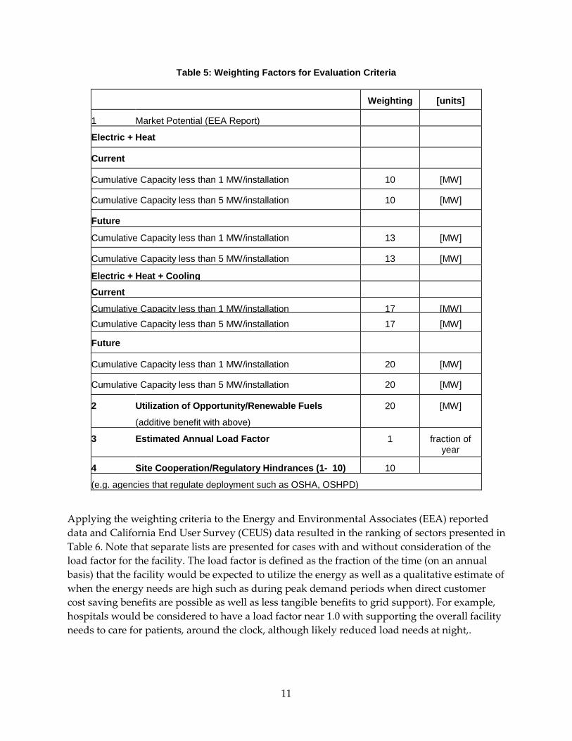
Table 5: Weighting Factors for Evaluation Criteria
Weighting [units]
1 Market Potential (EEA Report)
Electric + Heat
Current
Cumulative Capacity less than 1 MW/installation 10 [MW]
Cumulative Capacity less than 5 MW/installation 10 [MW]
Future
Cumulative Capacity less than 1 MW/installation 13 [MW]
Cumulative Capacity less than 5 MW/installation 13 [MW]
Electric + Heat + Cooling
Current
Cumulative Capacity less than 1 MW/installation 17 [MW] Cumulative Capacity less than 5 MW/installation 17 [MW]
Future
Cumulative Capacity less than 1 MW/installation 20 [MW]
Cumulative Capacity less than 5 MW/installation 20 [MW]
2 Utilization of Opportunity/Renewable Fuels
(additive benefit with above)
20 [MW]
3 Estimated Annual Load Factor 1 fraction of year
4 Site Cooperation/Regulatory Hindrances (1- 10) 10
(e.g. agencies that regulate deployment such as OSHA, OSHPD)
Applying the weighting criteria to the Energy and Environmental Associates (EEA) reported data and California End User Survey (CEUS) data resulted in the ranking of sectors presented in Table 6. Note that separate lists are presented for cases with and without consideration of the load factor for the facility. The load factor is defined as the fraction of the time (on an annual basis) that the facility would be expected to utilize the energy as well as a qualitative estimate of when the energy needs are high such as during peak demand periods when direct customer cost saving benefits are possible as well as less tangible benefits to grid support). For example, hospitals would be considered to have a load factor near 1.0 with supporting the overall facility needs to care for patients, around the clock, although likely reduced load needs at night,.
11

Conversely, retail stores and commercial office buildings would have virtually no load after closing time. In fact, commercial office buildings were assigned a load factor of only 0.33 representing an average of 11 hours of operating time per week day.
From the list presented in Table 6, further sector considerations such as anticipated cooperation and acceptance of the technology, generic nature of the sector definition, nominal size of the installation as compared to the definition of distributed generation were considered. For example, hospitals and healthcare are considered to be prime candidates for DG/CHP. However, the state agency that regulates hospitals, the Office of Statewide Health Planning and Development, (OSHPD) has generally displayed an aversion to the application DG/CHP technology which would negatively impact the perceived success of penetrating this market with DG/CHP. Additionally, while the Industrial / Chemical application opportunities would seem to be a prime candidate, the advisory panel deemed both to be too broad a categorization, making it difficult to identify a “typical” industrial or chemical process that could be monitored for evaluation. Rather, the industrial/chemical sector could form the basis for a study unto itself, with multiple processes evaluated.
12

Table 6: Ranking of Sectors Inclusive of Annual Load Factor Consideration
1. Hotel
2. Food/Restaurant
3. Commercial office
4. Hospital
5. Chemical
6. Nursing Home
7. Water/Sanitary
8. Prisons
9. College University
The ranked results presented in Table 6 reveal many sectors that are intuitive (hotels, hospitals) while identifying others that are not so obvious (food/restaurant). The TAC was unsure how to interpret the restaurant subsector’s standing. Further, it was difficult for the committee to fully understand how to monitor such a facility. Hence, the “food” aspect was retained in the form of grocery store and food distribution warehouses but “restaurants” were eliminated as a sector. In general, facilities that house and cater to people were seen as more applicable to the DG/CHP strategy owing to the care and comfort issues. Commercial office buildings and colleges and universities are a bit atypical owing to their diurnal operation (most have reduced or no population outside of operating hours). The food sector is a definite outlier in the corollary but the need for 24/7 operations for distribution, to keep the shelves stocked, and the cooling loads to keep food preserved presented a large opportunity. As a result of discussions with the TAC, the number of sectors was reduced to six as defined in Table 7.
13

Table 7: Final Sectors Chosen for Monitoring
Colleges/Universities
Commercial Office Building
Food Processing/Warehousing/Grocery Stores
Hospitals/Healthcare/Nursing
Hotels
Jails/Prisons
2.1.3 Site Evaluation With the sectors defined, establishment of criteria for the evaluation of specific sites within the sector were established (Table 8).
Much of the site evaluation occurred by effectively prequalifying sites based upon many of these attributes prior to approaching the facility.
Table 8: Site Evaluation Criteria
Site Analysis
• Suitable Size for Monitoring - Too large = $$$ equipment
• Proximity - Location relative to UCI, close proximity is easier to monitor and tend to problems
• CHP utilization – what specific CHP utilization is possible
• Existing On-Site Power Generation - Program calls for mix of sites with existing DG
• Number of Circuits to Monitor - More circuits = more equipment
• Accessibility of Communications
• Site Cooperation/Risk Aversion
• Potential for CHP integration in future
14
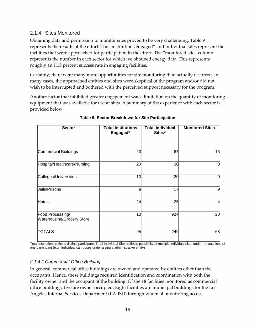
2.1.4 Sites Monitored Obtaining data and permission to monitor sites proved to be very challenging. Table 9 represents the results of the effort. The “institutions engaged” and individual sites represent the facilities that were approached for participation in the effort. The “monitored site” column represents the number in each sector for which we obtained energy data. This represents roughly an 11.5 percent success rate in engaging facilities.
Certainly, there were many more opportunities for site monitoring than actually occurred. In many cases, the approached entities and sites were skeptical of the program and/or did not wish to be interrupted and bothered with the perceived support necessary for the program.
Another factor that inhibited greater engagement was a limitation on the quantity of monitoring equipment that was available for use at sites. A summary of the experience with each sector is provided below.
Table 9: Sector Breakdown for Site Participation
Sector Total Institutions Engaged*
Total Individual Sites*
Monitored Sites
Commercial Buildings 23 67 18
Hospital/Healthcare/Nursing 20 30 8
Colleges/Universities 10 20 9
Jails/Prisons 8 17 9
Hotels 24 25 4
Food Processing/ Warehousing/Grocery Store
10 90+ 20
TOTALS 95 249 68
Total Institutions reflects distinct participant, Total Individual Sites reflects possibility of multiple individual sites under the auspices of one participant (e.g., individual campuses under a single administrative entity)
2.1.4.1 Commercial Office Building In general, commercial office buildings are owned and operated by entities other than the occupants. Hence, these buildings required identification and coordination with both the facility owner and the occupant of the building. Of the 18 facilities monitored as commercial office buildings, five are owner occupied. Eight facilities are municipal buildings for the Los Angeles Internal Services Department (LA-ISD) through whom all monitoring access
15

arrangements were made. Another eight facilities are owned by The Irvine Company through whom all monitoring access arrangements were made.
2.1.4.2 Hospitals/Healthcare/Nursing This sector was moderately well represented in the program with an outreach to approximately 30 sites. Most private hospital facilities did not want to participate in the program. Hospital facilities were very wary of the proposed program; while initially embraced by many of the facility managers/directors of engineering, upper level approval was never forthcoming. A specific explanation was never provided by any facility other than “We are not interested”.
However the perception is that the hospital and healthcare industry is highly regulated and heavily scrutinized; as such, there is likely a desire to keep a low profile and not have additional information on hospital operations disseminated. In addition, the California OSHPD, a state agency that oversees hospital operations and safety, has not generally embraced DG/CHP. While the latter does not necessarily preclude energy monitoring of a facility, it does affect the perception of the value of the monitoring effort if the goal is to assess the application of DG/CHP in a sector that has a low likelihood of penetration/application.
The hospital facilities that did participate were Federal Veteran’s Administration (VA) hospitals and one University of California “teaching” hospital. In addition, two health care clinics/centers operated by the LA-ISD were included.
2.1.4.3 Colleges/Universities Three campuses were included in the study; University of California Irvine (UCI, Cal State University Northridge (CSUN), and Pasadena City College (PCC). These three represent the three levels of the College and University system of higher education in California; research university, educational college, and community college respectively. For UCI, the campus as a whole was monitored as well as the energy needs of a variety of campus buildings that represent classrooms and research facilities. For CSUN and PCC, individual building performance was not assessed, only the campus as a whole. The community college sector was to have included the nine campuses of the Los Angeles Community College District (LACCD). Enthusiastic to participate, the access agreements were established; however, a combination of a lack of monitoring equipment and a general system wide construction effort including upgrades to central plant facilities precluded inclusion of any sites in the program.
2.1.4.4 Jails/Prisons The jail and prison sector proved vexing. Access to the state prison grid electric energy data was made available but it was subsequently discovered that 1) time resolved gas consumption data was not available and (2) generally, state jails and prisons are not air conditioned. Electric data was gathered for a number of California Department of Corrections facilities in Southern California Edison (SCE) territory through a web based account. The program was never able to physically install equipment at facilities. With just time resolved electric data available for jails and prisons, the value of this one aspect of the overall operation is dubious. Time resolved gas data for the likely highly cyclic nature expected (i.e. shower, laundry, food preparation) was not obtained.
16

Access to Federal prison information was never established. Attempts through the Federal Energy Management Program (FEMP) office were not successful.
One type of facility included in the sector is State Mental Health Hospitals. While officially considered hospitals, these facilities are arguably a variation on prisons, with the majority of the patients being criminals that are undergoing mental health evaluation or are not considered fit for trial. Unlike state prisons, the Mental Health hospitals provide lower density occupancy that included air conditioning. As State Prisons are expected to install air conditioning for prisoner comfort in coming years, the performance of the State Mental Hospitals provides a reasonable prediction of the coming needs as these facilities do have air conditioning for the residents. The program monitored Patton State Hospital (San Bernardino) and Metropolitan State Hospital (Los Angeles/Norwalk).
2.1.4.5 Hotels Hotels hold promise as another very fine match for DG/CHP. Much like hospitals, the “hospitality” services of food and comfort lodging would seemingly translate to high energy intensity nearly 24/7. However, the sector is very competitive and reluctant to share or provide access to information on the day-to-day operations which could be considered competition sensitive. As such, while more than25 hotel sites were approached, only four were monitored. And of the four, one was a high rise residential facility for the US Navy in San Diego that does not have the same level of hospitality service as a conventional hotel.
2.1.4.6 Food Processing/Warehousing/Grocery Stores For the food sector, the efforts predominantly focused on grocery stores. Five grocery store chains were approached. Two chains agreed to participate. Stater Brothers agreed to provide access to four of its stores for instrumentation distributed between temperate and hotter climate areas. A second chain wishing to not be identified provided energy data from their energy management system for the overall energy consumption as well as subsets that included lighting and refrigeration for 14 of their stores in both Southern California, Las Vegas, and Arizona (while outside of California, the latter two to provided high ambient temperature performance for comparable buildings). The US Navy Commissary at the Naval Base, San Diego, representing a state of the art facility with many energy savings measures incorporated, was included. Finally, a single large scale food distribution warehouse with multiple levels of refrigeration for food preservation was also included. No food processing facilities participated in the program despite approaching several in the SoCAB.
17

CHAPTER 3: Thermal and Electric Demand Measurements Measurement of the thermal and electrical demand comprises the majority of this research activity. The general approach was to treat each facility as a black box and monitor the energy crossing the boundary of the black box from utilities (electric and natural gas) as well as energy provided by any on-site power systems such as photovoltaic and DG/CHP systems. For the latter, the energy crossing into the black box would also include any thermal energy, either hot water or chilled water, captured through waste heat recovery from a DG/CHP system. Beyond the energy crossing the boundary of the black box, information on energy consumption within the box was of interest. Specifically, the loads for heat and cooling in support of the HVAC system and/or other process heating and cooling loads that could be partially or fully met using waste heat recovery and thermally activated cooling technologies (e.g. absorption and adsorption chilling) were identified. The goal was to understand the effective and efficient application of DG/CHP to meeting building energy needs both thermally and electrically as well as assess the impact of the DG/CHP on the overall energy profile for the facility.
One of the key questions addressed early on was the time scale of the monitoring. Initially, data was to be gathered at very high resolution (on the order of 3-sec intervals). Measurements have shown very large energy demand spikes that are not captured in long interval monitoring.
However, the TAC argued that (1) DG/CHP would not eliminate the grid, (2) the grid would be present to handle any high load transients, and (3) a DG/CHP system could not respond to perturbations that would occur in the order of seconds. Rather, the TAC recommended a measurement interval of 15 minutes to correspond with the sampling rate resolution of utilities and the supplied grid electricity. This does provide a data manipulation benefit of reducing the number of lines of data to slightly more than 35,000 lines of data per year as opposed to more than 10 million lines of data at 3 second intervals.
The initial thoughts for the monitoring strategy at sites included:
• the installation of a power meter on the point of common connection between the facility and the utility electric grid,
• installation of a natural gas flow meter on the gas supply, and
• installation of a metering equipment to monitor the heat energy transport (measured in British Thermal Units (BTU) provided by the hot water and the chilled water loops.
18

However, the reality of implementing the instrumentation resulted in some deviations from this scenario for the sake of safety, accuracy, expediency, and equipment supply limitations. One of the key issues encountered was the inability to install instrumentation in desired systems without requiring a facility operations interruption or shut-down, a prospect no site was willing to undertake. Re-evaluating the needs and availability of information from other sources, plans were specifically
• Where ever possible, existing facility energy management system (EMS) data were utilized once confirmed to be accurate.
• Use of utility recorded information via access to the facilities account and website based data. This has been implemented in virtually all cases, either through UCI having direct access to the account information or the facility providing the data from their utility account.
• Natural gas consumption was based upon monthly utility bills where available. With only one exception, there was not time resolved facility natural gas consumption information available. Southern California Gas, the gas utility for all of the sites in this program, does not provide time resolved metering as a general practice. We also discovered that there are rarely (never) any inherent access ports in the supply line where monitoring equipment could have been installed without a system shutdown and significant plumbing modifications made. As such, heating loads identified are the result of either (1) direct measurement of the hot water needs or (2) operational history of the boiler and assumptions of firing rate based upon nameplate data. Also, in general, the domestic hot water (DHW) consumption was not directly measured. For some facilities, the DHW was provided by part of the overall boiler/hot water loop and could not be separated. For other facilities, hot water was provided by local electric hot water heaters at the point of use. The operation of individual tank hot water heaters was not monitored.
• Air conditioning systems based upon direct expansion (DX) systems (i.e. roof-top AC systems) did not fit the model of measuring chilled water flow and temperature rise. For facilities that utilized the DX systems, the electric energy consumed by the unit was monitored. Based upon nameplate data for the equipment, the fraction of energy associated with the compressor (not inclusive of the fan) was calculated and the manufacturer’s coefficient of performance for the chiller utilized to ascertain the chilling load.
3.1 Utility and EMS Data Electric utility data for the primary electric feed to the facilities was obtained for virtually all facilities. This was accomplished either through: (1) the facility providing the data via their gathering of the data from the Utility website, (2) the data was available from the site’s EMS data logs, or (3) the facility provided UCI with account access and we recovered the data from the Utility. Direct measurement of the primary power was performed at only two sites because other facilities were not willing to shut-down or otherwise interrupt their operations for a full
19
building electric shutdown necessary to install the monitoring equipment. The desired 15 minute interval data were gathered as a matter of course by the utility for all sites with time of use metering. All of the data obtained from the utilities was energy consumption (e.g. kilowatt- hour (kw-hr)) for 15 minute intervals. In general, natural gas consumption, if obtained, was based upon monthly bills. SoCal Gas does not customarily monitor gas consumption based upon the time of day so utility based data is limited to monthly consumption. For most instances, this was not a major issue as large sources of heat (boilers, large hot water systems) were individually monitored. The belief is that the majority of the heating loads that would have been provided by natural gas were captured through the monitoring of the individual systems.
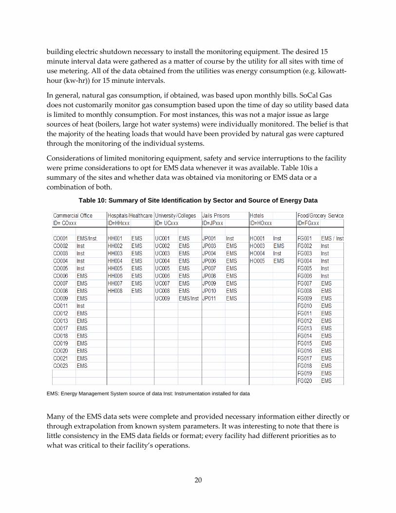
Considerations of limited monitoring equipment, safety and service interruptions to the facility were prime considerations to opt for EMS data whenever it was available. Table 10is a summary of the sites and whether data was obtained via monitoring or EMS data or a combination of both.
Table 10: Summary of Site Identification by Sector and Source of Energy Data
EMS: Energy Management System source of data Inst: Instrumentation installed for data
Many of the EMS data sets were complete and provided necessary information either directly or through extrapolation from known system parameters. It was interesting to note that there is little consistency in the EMS data fields or format; every facility had different priorities as to what was critical to their facility’s operations.
20
3.2 Equipment Installation For sites that required instrumentation, a wide variety of monitoring equipment and recording equipment was utilized, depending upon the specific site needs and proximity of subsystems.
3.2.1 Electric Energy Electric energy to the facility from utilities was anticipated to be monitored independently at each site. However, it was quickly determined that instrumenting of the main electric feed would be highly problematic; rather, in virtually all cases, existing and installed electric meters (utility or site sub-meters) would provide sufficient information. The utility meters were accessed through web based data provided by the utility to their customers. The data varies somewhat from utility to utility but in general, information on energy consumption at 15 minute intervals was available. This is the same data set that the utilities use for billing of the customer. As such, the accuracy of the meter can be considered revenue grade certified with an accuracy error of less than 1percent of the reading. For some sites, primarily those with photovoltaic systems, on-site power generation was also monitored by the utility and available through the same utility supported data base.
Beyond the grid electric, the need for monitoring of electric power consumption was nearly universal at all sites. Small self-contained power monitoring systems (described below) with voltage taps and split core current transformers proved to be the easiest to implement and could, with care, be installed with no service disruption and with no facility alterations. Electric system monitoring consumption was used to monitor the energy flow for chillers, DX air conditioners, refrigeration systems, and sub-metering of buildings. In two cases, these power meters were used for monitoring the primary electric energy flow into the facility. Two systems are available for use, depending upon the site needs but both utilized the same principles of current transformers (for this study, split core transformers that permitted installation without lift the leads (i.e. without service disruption)) monitoring the current flow and voltage taps monitoring the voltage on the supply conductors. Without exception, all of the electric service to the facilities and to the primary loads monitored was 3-phase. The service voltage varied among sites but was either 208 volt or 480 volt.
3.2.1.1 Dent Elite Pro Power Meter The Dent Elite Pro power meter (Dent)10 was the primary system of choice. The system is very flexible for a wide variety of electric service configuration and voltages and with proper choice of the Dent proprietary current transformers, offers a wide range of power monitoring levels. The system operation is configured though a computer interface that allows the user to choose electric circuit configuration parameters, specify the current transformer size, the logging rate and the parameters of interest with includes individual leg and cumulative data on voltage and current (average, maximum, minimum) as well as power (kW, kVA, kVAR, power factor). The Dent Elite Pro meter also provides on board data logging. When equipped with an extend memory option (as was done for this program), the units could store more than 2 years’ worth
10 Dent Meter, Bend OR; www.dentinstruments.com
21

of data (depending upon the number of fields being recorded). The data is retrieved from the meter via the same communications system used for configuring the system through the computer. The stated accuracy of the Dent Power Meter for energy/power values is less than 0.5 percent of reading
3.2.1.2 Flex-core Power Meter The Flex-core power meter (Flexcore)11 (model WL50-346-500K) was identified as a lower cost alternative to the Dent Elite Pro Meter. This meter is set for a fixed voltage and current limit and does not provide on board data logging. The device provides a pulse output corresponding to a specific energy. As such, this meter was limited to applications wherein additional data was to be monitored and logged through the Campbell Scientific multi-channel data logging system (see Section3.2.4). As a low cost alternative, the units proved to be reliable
if not flexible (the unit’s operating voltage and expected current range needed to be defined at time of purchase and were not adjustable as was the case for the Dent meters) and provided additional monitoring capability for facilities beyond what was possible with the number of Dent meters in the program. The stated accuracy of the Flex-core Power Meter is less than 1percent of reading.
3.2.2 Water Flow / BTU Meters To monitor the performance of heating and cooling loops that were otherwise not instrumented, a water flow meter and temperature sensors to measure the change in temperature of the fluid were used. Knowing the mass flow of the water (through the measured volume flow) and the change in temperature, the energy change can be calculated.
3.2.2.1 Emco ST 30 Sono-Trak meter The primary goal of the instrumentation from the perspective of the facility was to not disrupt service. The Emco ST30 Sono-Trak meter(EMCO)12 is a non-intrusive ultrasonic flow meter that is mounted to the outer surface of the pipe containing the fluid. Ultrasonic waves are “bounced” between two transducers that are set a specific separation (dependent upon the fluid, pipe thickness, and the pipe diameter), both with the flow and against the flow. Through analysis of the received frequency, the bulk fluid velocity can be calculated. Further, the system can, through the input of pipe parameters, will calculate a volumetric flow rate and accumulate total volume reading. The system provides a 4-20 mA output proportional to the flow rate that must be recorded via the data logger. The stated accuracy of the Emco ST 30 is less than 2 percent of the flowrate reading in a field application; repeatability is less than 0.5 percent.
11 Flex-Core, Milliard, OH; www.flex-core.com
12 Engineering Measurements Co., Longmont CO; www.emcoflow.us
22
Two downside issues with the system were:
1. The need to establish a uniform flow through the metering field. This mandated a minimum length of straight uniform pipe upstream and downstream of the monitoring point. This proved challenging in many installations given the typically tight space within mechanical rooms and the circuitous routing of the plumbing
2. The need to have the meter mounted directly to the pipe for proper acoustic coupling. This required the removal of installed insulation on the piping. Great care was required to minimize the amount of material removed and to retain the insulation so that it could be replaced at the conclusion of the monitoring effort.
The meter proved to be reasonably reliable but some instances of erroneous readings were observed, perhaps the result of contamination or more likely air bubbles in the flow field.
3.2.2.2 Temperature Monitoring In conjunction with the flow meter, the change in fluid temperature entering and exiting either a boiler or a chiller is necessary to calculate the change in energy. In the spirit of non-invasive measurements, surface mount devices were incorporated. These were either 100-ohm RTD (resistance temperature devices) with an adhesive pad substrate or a magnetically mounted type T thermocouple. Both were connected to transmitter devices that converted their inherent signal to a 4-20 mA signal that was logged. One interesting and unexpected development was an electrical interference for the magnetic mounted thermocouple; a single device could be mounted and accurate data received; however, two or more devices that were electrically connected (i.e. the piping is an electrical conductor) resulted in erroneous readings. We were never able to determine the reason but assumed it was the result of ground loops or magnetic mount induced electromagnetic interference (EMI).
For the low profile RTD, the device was tucked under some of the existing pipe insulation; the expectation being that near steady state with insulation, the surface temp of the pipe would be nearly equivalent to and track the changes in the fluid temperature. For the larger thermocouple mount, insulation was packed around the device to minimize any heat loss through the surface of the piping.
For both the thermocouple and the RTD, standard “commercial” tolerance devices were utilized. As such, typical errors for RTD’s and thermocouples apply.
3.2.3 Gas Flow Overall natural gas consumption at a facility was typically limited to readings provided on monthly utility bills. Typically, natural gas provided by the utility is not “time of use” sensitive and as such, the installed meters do not normally have a means for providing time resolved consumption history. Further, natural gas supplies to a facility are the property of the utility until the discharge point of the meter so alteration to the plumbing to permit installation of time resolved metering upstream of the meter is not viable. Finally, meter discharge is typically positioned immediately adjacent to the building. Once entering the building, the plumbing is
23
generally not accessible and does not include access ports. Therefore, any facility natural gas consumption reported is the result of monthly total consumption readings.
The lack of time resolved facility wide gas consumption is not a major issue. Internal systems that utilize the waste heat for heating purposes such as HVAC heating and process steam were monitored separately and individually and an assessment of the heating needs documented.
Other facility systems that consume gas (i.e. kitchen cooking, laundry dryers, etc.) are loads that are not easily nor directly addressed by a DG/CHP system. Hence, even without a fully time resolved overall facility natural gas consumption history, specific metering of the HVAC loads which can be addressed by a DG/CHP system was captured.
Sage SGI (SAGE)13 insertion thermal mass flow meters were used to monitor natural gas flow where necessary. The meter utilizes the principle of heat loss from a heated temperature device to calculate the true mass flow of gas which is correlated to and reported as a “standard” volume flow. The device provides a 4-20 mA signal proportional to the flow rate and is recorded by the data logger. The stated accuracy for the Sage SGI meters is less than 1 percent of reading with a repeatability of 0.2 percent of full scale value.
The Sage meters were purchased pre-calibrated for natural gas. They were rated for piping from 2” ID minimum to up to 18” diameter. The thermal sensors are designed to be located in the center of the pipe flow. As with the water flow meter, pipe parameters are input to correlate the mass flow to the volumetric flow. Also like the water meter, the device wants uniform flow field upstream and downstream of the meter. A proper section of pipe was usually easier to identify than the water meter. However, unlike the water system, the gas flow meter was inserted into the flow. This required locating or installing an access port in the piping as well as a both a gas service shutdown. The use of these meters was limited to facilities with on-site fuel based distributed generation system (i.e. microturbines or fuel cells) that did not have existing fuel monitoring. We were never able to identify an application of the meter to monitor facility level gas flow rates.
3.2.4 Data Logging For all signals from devices other than the Dent Elite Pro power meter, data was retrieved and logged with Campbell Scientific Data loggers (Campbell)14. Both CR 1000 and CR 800 devices were utilized depending upon the number of channels to be logged. Both devices are capable of logging voltage signals and, with external shunt resistors, current signal inputs. They are also able to monitor pulse inputs (such as those from the Flex-core power meters). While capable of remote access via phone modem or wireless modem connections, all data was manually downloaded from the devices. At the sampling frequency of 15-minutes, the internal memory provided many months of data capacity.
13 Sage Metering Inc, Monterey CA; www.sagemetering.com
14 Campbell Scientific Inc., Logan UT; www.campbellsci.com
24

The Campbell Scientific data loggers utilize 13- bit A-D converters (± 0.06 percent resolution) for storing the analog voltage signals that are compatible with the logger. For current signals, precision resistance “shunts” of 100 ±0.01% resistors are used to convert the signal to voltages.
For the parameters being measured as part of this program, the precision of the sensors is in line with the ASERTTI field testing and long term monitoring protocol specifications (Table 11).
Table 11: Comparison of Measurement Accuracy with ASERTTI Protocols
Parameter Units ASERTTI Field Test
ASERTTI Long Term
CEC Energy Monitoring
Electric Power Kw-hr ± 0.6% of reading Value of ±0.25 ± 0.6% of reading
Gas Consumption scf or MMbtu ±1% reading ±1% full scale ±1% of reading
Waste Heat
Fluid Flow Rate Gallons per minute
±1% reading Calculated btu recovery based upon all parameters: ± 10%
±2% reading
Fluid Temperature ° F ±0.6 °F of
temperature
±1 °F of temperature
Fluid density and specific heat
lb/cu-ft Btu/lb ±0.11%
±0.16%
± 0.2%
±0.1%
Assumed to be water
25
CHAPTER 4: Data Base Generation 4.1 Data Base Architecture The data base is oriented around the structured query language (SQL) protocol. SQL is inherently suitable for large data base storage and manipulation. The data base will consist of a single level table of data identified by sector and site identification serial number. The structure of the table and the characteristics of the SQL protocol will permit interrogation of the data for individual sites as well as comparative interrogation within sectors and across sectors.
For the monitoring effort, the monitored facilities are treated as a “black box” in which energy crosses the boundary in the form of grid electricity and natural gas. Additionally, the energy needed to provide HVAC cooling and heating (i.e. occupant comfort) and process cooling and heating (i.e. process cooling and heating) are monitored coincident with the energy crossing the black box boundary. The cooling and heating components are expected to be energy loads that can be addressed with waste heat recovery strategies from DG systems. A comparison of the heating and cooling loads versus the electric energy needs is used to identify the DG/CHP technology that is best matched to the needs. The data base includes ambient condition information, energy consumption data for the site, including energy input to the facility crossing the facility boundary (i.e. natural gas and grid supplied electric) as well as any on-site power generation through the application of fuel based systems (i.e. microturbines, fuel cells) or non-fuel based (i.e. photovoltaic), and information on the use of the energy within the facility boundary that could potentially be met through the application of waste heat recovery, specifically HVAC heating and cooling, DHW heating, and any process heating and cooling needs.
Aside from data obtained from the monitoring effort itself, the data base includes ambient conditions (dry bulb temperature and relative humidity) to permit trending and comparison of the energy needs with respect to the prevailing weather conditions. Finally, the data base includes a number of parameters that are calculated based upon site characteristics; that is, several data points will be normalized to permit comparison of the energy intensity of the facility within and outside of its sector with other facilities.
4.2 Fields As a result of the monitoring effort of this program, a time dependent data record was obtained from each site for the total energy consumption for the facility as well as the energy requirements for HVAC needs and process loads. In addition, for the sites that have an existing on-site generation/co-gen installation, information on the energy produced, energy consumed (if any), and the amount waste heat recovered was recorded.
Many of the sites in this effort have multiple inputs for the desired parameters. For instance, some installations have multiple electric meters feeding the facility, have multiple air conditioners, and/or have multiple distributed generation systems on site. The disparate and
26

unique nature of each site’s energy monitoring history would make interrogation of the final SQL data base cumbersome and comparison virtually impossible. As such, the individual data sets are processed and summarized into single “totals” for presentation in the SQL database in a consistent format with consistent field headings.
In addition to processing the data from multiple monitoring points into a consistent set of facility parameters, the data were further processed to provide information on the sub-metered loads as compared to the total energy. Further processing of the data resulted in reporting of some benchmark data normalize the energy consumption based upon some facility characteristics such as square footage, occupants, and/or number of rooms.
For those sites with existing on-site generation/co-generation systems, one goal of the program was to provide time resolved history of system electrical and, if outfitted, waste heat thermal recovery output as well as fuel to electric and fuel to thermal efficiencies. Since their presence offsets the facility’s electric energy consumption from the grid, any on-site energy production was added to the monitored energy consumption from the grid and reported as the total site energy requirement. The contribution of the on-site power generation was tabulated individually as well as a calculated percentage of the electric power to the total demand.
Similarly, if the contribution of a waste heat recovery system offsets a chilling or heating load provided by a more conventional electric chiller, boiler, or furnace, the contribution of the co- generation was added to the monitored chiller or heater performance as appropriate to provide a total facility chiller/heater/process demand for the facility. As with the electric power, the contribution of the co-generated heating/chilling/process load was reported individually as well as calculated percentages of the total demand.
4.2.1 Site Reporting Fields The specific data fields reported in the SQL data base are presented below and in Table 12. The units and format of the data is presented in the “[ ]”. Any additional comments relative to the parameters are presented in italics within the “( )”. A total of 64 columns of data are populated:
• Site ID; [sequence number]
• Date Stamp; [date/number]
• Time Stamp; [time number]
• Ambient Temp; [deg F, number]
• Relative Humidity; [%, number]
• Total Electric Energy for time interval; [kw-hr, number] (summation of any individual meters for the site and any on site power generation from combustion, fuel cell, and/or PV).
• Total Gas Consumption for time interval [btu, number]; (for many facilities, the gas consumption will be quite small, serving essentially DHW and some HVAC. Depending
27

upon magnitude of number, this may be measured or a calculated number based upon heat production or system operation and nominal firing rate)
• Total HVAC Chilling for time interval; [btu, number] (summation chilled water and/or direct air cooling)
• Total HVAC/DHW Heating for time interval; [btu, number] (summation of all heating for HVAC and domestic hot water)
• Total Process Chilling for time interval; [btu, number] (summation of any chilling loads outside of HVAC (e.g. refrigeration for grocery stores))
• Total Process Heating for time interval; [btu, number] (summation of any heating loads outside of HVAC and DHW (e.g. process steam for sterilization); note that this would only be associated with systems that make the steam or hot water directly. Many restaurants/hotels/hospitals take the same hot water used for HVAC and locally heat for the need such as internal/integral electric heater for dishwasher or autoclave. We cannot monitor these minor loads)
• Total Fuel Based On-Site Electric Power Generated for time interval; e.g. microturbine, fuel cell; [kw-hr, number]
• Total Non-Fuel Based On-Site Electric Power for time interval; e.g. solar, wind; [kw-hr, number]
• Total end use waste heat recovery for time interval; [btu, number], (this would be a measure of the end use of the waste heat recovery accounting for any losses/inefficiencies in conversion of waste heat to a beneficial commodity). Applicable for:
o Total Waste Heat to Hot Water/Steam; [btu, number]
o Total Waste Heat to Chilling; [btu, number]
o Total Waste Heat to “Other”; [btu, number] (dehumidification, direct to process use, others to be defined)
• Efficiency Fuel to Electric [% on LHV, number] (LHV = lower heating value of fuel)
• Efficiency Fuel to Electric + Thermal; [% on LHV, number], (combine the total electric energy with useful thermal recovery in consistent units)
• Percentage/Ratio of chill or heat to total electric energy consumed; [%, number] for time interval (all calculated values) (Note, limiting to electric since this would be the parameter of interest and parameter offset with the application of DG technologies)
o HVAC Chill/Total Electric Energy o HVAC Heat/Total Thermal Energy o Process Chill/Total Energy
o Process Heat/Total Energy
28

• Normalized loads per square foot for time interval (each parameter divided by facility sq-ft)
o Total Electric [kw/sq-ft, number]
o Total Energy [btu/sq-ft, number] (gas and electric in consistent units)
o Total HVAC Chill [btu/hr/sq-ft, number]
o Total HVAC Heat [btu/hr/sq-ft, number]
o Total Process Chilling [btu/hr/sq-ft, number]
o Total Process Heating [btu/hr/sq-ft, number]
• Other Normalizations for time interval: Same parameters as above but normalized as follows for each of the sectors:
o Colleges/University: (normalized per number of students).
o Hospitals/Nursing Homes: (normalized per number of beds)
o Hotels: (normalized per number of rooms and/or number of beds).
o Jails/Prisons: (normalized per number of actual inmates)
o Commercial Buildings: (normalized per nominal number of occupants/employees)
o Food/Grocery: (no other normalizations expected)
4.2.2 Site Characteristics Template Beyond the monitored site energy data, site characteristics were gathered to provide background and the basis for comparison with other facilities. Figure 1, Figure 2, and Figure 3 present a typical, three page site template utilized for this program. Note that very specific information was requested regarding utility accounts and costs. In the end, no site provided this information. In as much as rates are fluid and specific account information is not immediately relevant to the study, this was not considered an issue.
The site templates did request information on the gross square footage of the facilities served by the electric meters and the other monitored loads. Information on occupancy was also requested. However, in many instances, such as hotels and commercial office, this number varies widely and continuously. Of note is the effect of the economic duress that was prevalent during the period of this effort. Some of the commercial office space and the hotels that participated experienced below normal occupancy levels and as a result, the data obtained can be considered skewed to lower levels or perhaps higher per capita levels than might otherwise be the norm.
29
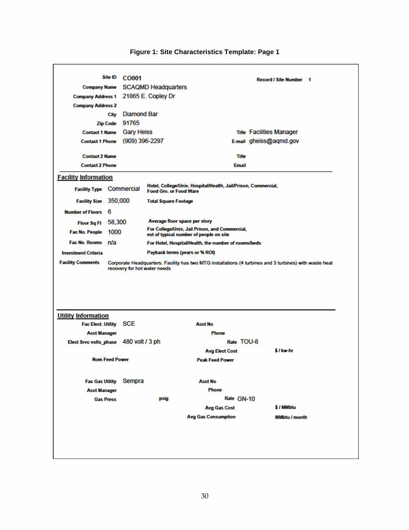
Figure 1: Site Characteristics Template: Page 1
30

Figure 2: Site Characteristics Template: Page 2
31

Figure 3: Site Characteristics Template: Page 3
4.2.3 SQL Data Base Hosting and Use CEC Monitoring data is available as a SQL Server 2008 database. The data was consolidated in one large table named “CEC_Table.” The database is hosted on APEP premises in a dedicated instance. The data stored in this instance is read-only and can be accessed by following these steps:
Connect to SQL Server 2008 CECDB instance:
IP address: 128.200.20.231
TCP Port: 51433
Username: cecuser
Password: apepcec2102
Database: CECDB-V1
The easiest way to connect to the SQL Server is to create a SQL Server alias. The follow link is a tutorial to create an alias: http://sqldbpool.com/2011/01/07/how-to-create-alias-in-sql-server/
32
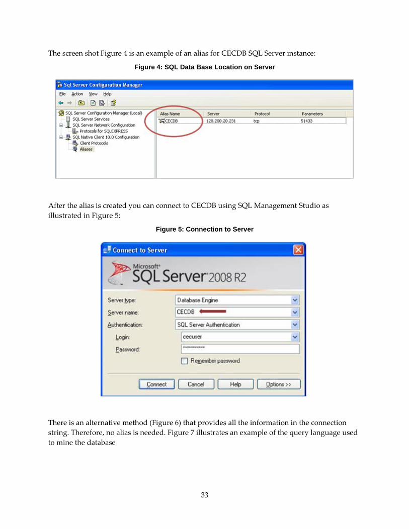
The screen shot Figure 4 is an example of an alias for CECDB SQL Server instance:
Figure 4: SQL Data Base Location on Server
After the alias is created you can connect to CECDB using SQL Management Studio as illustrated in Figure 5:
Figure 5: Connection to Server
There is an alternative method (Figure 6) that provides all the information in the connection string. Therefore, no alias is needed. Figure 7 illustrates an example of the query language used to mine the database
33

Figure 6: Alternate Connection Scheme
Figure 7: Sample Queries Using T-SQL
34
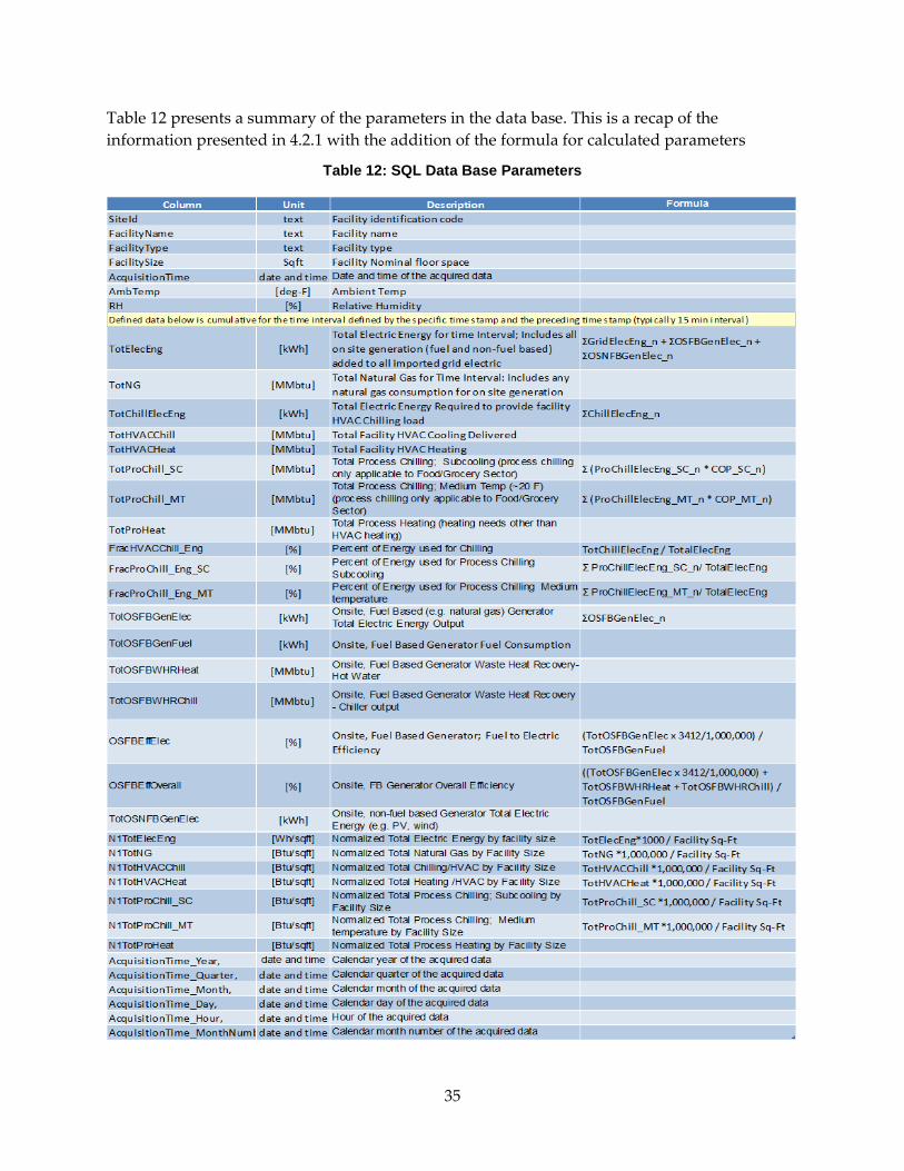
Table 12 presents a summary of the parameters in the data base. This is a recap of the information presented in 4.2.1 with the addition of the formula for calculated parameters
Table 12: SQL Data Base Parameters
35

4.3 Preliminary Review and Comparison of Energy Profiles 4.3.1 Commercial Office The results for a large commercial office facility are present inFigure 8 and Figure 9. This facility, located in Irvine, CA, has total floor space of 1.12 million square feet spread over 5 buildings and a total of 54 stories. The facility is unique in the application of a chilling only central plant of 1500 tons total capacity as well as a thermal energy storage capability for chilled water of 12,500 ton hours. Space heating and domestic hot water needs are addressed through local electric resistance heating.
A typical summer day is shown in Figure 8. The electric energy for the site at 15 minute intervals (kw-hr) inclusive of the chilling loads is shown as is the building chilled water demand for HVAC needs (refrigeration ton-hr).
As a possible scenario of application of a DG/CHP system, assume that the chilling demand could be met with a double effect absorption chiller sized for 300 tons coupled with a 1.5 MW gas turbine. Further, assume that the gas turbine has a minimum load capability of 70 percent of the full load (i.e. 1.0 MW). The result of this scenario is presented in Figure 9. Note that the turbine would only operate during typical business hours (6 am to 6 pm) but during that time, all of the chilling loads are met either through the thermal energy storage system or the absorption chiller, the grid imported peak electric power is reduced by 87 percent and the electric energy is reduced by 62 percent. Another possible scenario, not presented here, is application of the DG/CHP to meet the 24hr baseline demand (i.e. provide electric power and cooling overnight to recharge the thermal energy storage tank). However, the impacts to the grid during the period of highest need (i.e. peak energy demand) and the resultant cost savings would be less than the scenario presented.
Figure 8: As Measured Typical Summer Energy Profile: Commercial Office Building
36

Figure 9: Energy Profile After Application of DG/CHP: Commercial Office Building
4.3.2 Grocery Store The results of the monitoring of a medium size grocery store during a typical summer day are presented in Figure 10 and Figure 11. This store, located in Laguna Hills, CA, has a nominal sales floor space of 29,000 sq-ft and ancillary space of approximately 14,100 for a total building size of 43,100 sq-ft. The facility has an installed capacity of air conditioning of 40 tons , subcooling of 20 tons, medium temperature refrigeration (> 20 deg F) of 35 tons, and low temperature refrigeration (<20 deg F) of 22 tons. The results of the energy monitoring indicated that the subcooling and medium temperature loads are nearly constant while the air conditioning load, owing to the relatively temperate climate and the spill over cooling from the other refrigeration systems operated less than 10 percent of the time.
Thermally activated cooling (e.g. absorption cooling) is limited to minimum temperatures of 40 deg F for lithium bromide systems and as low as 0 deg F for ammonia based systems. The former are typical for HVAC system applications but, in the case of grocery stores would also be applicable for subcooling where the temperatures needed are 60 deg F. For the ammonia based systems, the technology is well understood in as much as these were the first application of absorption technology; however, the danger associated with ammonia and the development of lithium bromide systems has resulted in a very limited number of suppliers of ammonia absorption chiller technology.
As a possible scenario of application of a DG/CHP system, assume that the medium temperature chilling demand which includes the air conditioning, and sub cooling loads could be met with an array of single effect absorption chillers sized for 75 tons total coupled with a 150 kW reciprocating engine (note that is presumes that an ammonia absorption chiller of could be applied for the medium temperature cooling needs in the 20 – 40 F range). Further, assume
37

that the reciprocating engine has a minimum load capability of 50 percent of the full load (i.e. 75 kW). The result of this scenario is presented in Figure 11 Note that the engine would be able to operate all day neither exporting electric power nor exceed the lower limit of its operating range. The DG/CHP would be able to meet virtually all of the energy needs for the facility through the day, only drawing upon the grid during the peak mid-day periods. The grid imported peak electric power is reduced by 88 percent and the electric energy is reduced by 95 percent. Further, assuming specific utility costs (Electric: SCE TOU-GS3, natural gas: $5.00 per MMbtu), a nominal utility cost savings of approximately $7000 (or 60 percent over the grid connected scenario) is possible.
This research has shown that the food and grocery industry which includes grocery stores and convenience stores (e.g. 7- Eleven), which currently has a very low use of DG/CHP, would be an excellent candidate for use of this system while reaping one of the highest efficiencies and smallest emissions footprint. In California as a whole, there are more than 5,600 food/convenience stores considered “medium” or “large” in the CEUS report (>=190 MW-hr annual and >=1,600 MW-hr annual) and representing approximately 5,100 GW-hr of energy consumption (ITRON)15. The results of this program indicate that a DG/CHP system typically meet greater than 90 percent of all of the energy demands at a food/grocery store with both the on-site electric power generation and the displacement of more than 50 percent of the refrigeration needs through the application of thermally activated cooling driven by waste heat. Further, the overall thermal efficiency of such a system would be greater than 75 percent and result in a net reduction in natural gas consumption of approximately 20 percent over a full grid feed for the electric power. The savings of 10.2 million MMbtu of natural gas would result in a reduction of 544,000 MT of carbon dioxide emissions annually. The result of the research in the program also indicates there is an engineering need that would further benefit the effective application of DG/CHP in the food and convenience market sector. Specifically, development and improvements in thermally activated cooling systems to support the medium temperature refrigeration applications are crucial to the potential for DG/CHP to provide the noted energy efficiency opportunities. In parallel, development and deployment of secondary fluid refrigeration systems at food/grocery stores are necessary to take advantage of the application of thermally activated cooling in this sector. Technology advances in this arena which will help the DG/ CHP industry to provide better products to meet California’s electricity generation goals.
15 ITRON Inc., California Commercial End Use Survey, March 2006; prepared for the California Energy Commission by Itron Inc, Report NumberCEC-400-2006-00
38

Figure 10: As Measured Typical Summer Energy Profile: Grocery Store
Figure 11: Energy Profile After Application of DG.CHP: Grocery Store
39

CHAPTER 5: Comparison of DG/CHP Utilization 5.1 Sites Identified The original intent for this program was to identify approximately equal numbers of facilities without on-site DG/CHP as with. Efforts in establishing site candidates did address this goal but, as it turned out, only four sites that agreed to participate in the program had on site DG/CHP systems. Specifically, these sites were:
• South Coast Air Quality Management District (SCAQMD) headquarters: 435 kW total; two installations with seven microturbines total – one 3 x 65 kW and one 4 x 60; both with waste heat recovery for hot water
• California State University Northridge (CSUN): 1 MW total fuel cell installation (four units) with some waste heat recovery for hot water. – 692 kW photovoltaic also on site.
• Pasadena City College (PCC): 240 kW total (4 x 60 kW) waste heat recovery for absorption chilling
• UC Davis Medical Center (UCDMC): 26 MW gas turbine/steam turbine combined cycle installation with waste heat recovery for additional electricity (steam turbine), HVAC heating and chilling (via absorption chiller), domestic hot water and process steam.
For the DG/CHP systems, fuel consumption, net electric power output and waste heat recovery/utilization was monitored on the program consistent 15 minute intervals. Each site has some unique features in their installation as described.
5.1.1 SCAQMD DG/CHP The SCAQMD has two separate installations of microturbines. One system (Figure 12) is comprised of a set of four Capstone 60 kW turbines and dates from approximately 2002. For clarity, this will be referred to as System 1. The units are grouped in sets of two, each set having the exhaust gas feeding a single MicoGen (e.g. two MicoGen heat exchangers for the four turbines) waste heat recovery heat exchanger to provide hot water. The second system (Figure13) is comprised of three Capstone 65 kW units with the exhausts ganged together and feeding a single Cain waste heat recovery heat exchanger to generate hot water. For clarity, this will be referred to as System 2. The hot water generated is used for facility HVAC heating needs throughout the year; the Central Plant chillers providing HVAC cooling and dehumidification with local reheat for comfort. This loop is parallel with the facility’s boiler system and offsets operation of the boiler. One unique issue with the AQMD waste heat recovery installation is the distance between the tie in point for the hot water for the building “loop” relative to the location of the microturbines themselves. The piping runs are approximately 300 ft long; the three turbine installation is predominantly underground while the four turbine plumbing is mounted to the exterior of the building. In both cases, the piping is insulated but both heat and pumping energy losses render this scenario less than ideal.
40
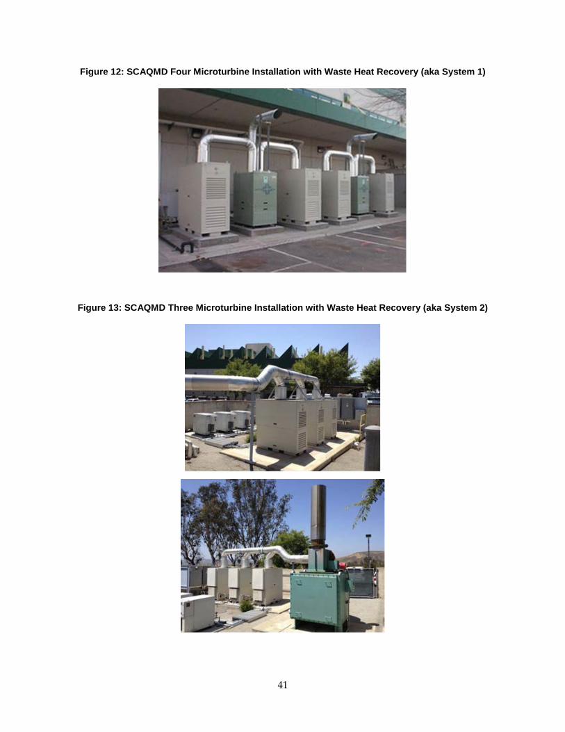
Figure 12: SCAQMD Four Microturbine Installation with Waste Heat Recovery (aka System 1)
Figure 13: SCAQMD Three Microturbine Installation with Waste Heat Recovery (aka System 2)
41

5.1.2 CSUN The CSUN campus is progressive in the application of DG/CHP as well as other renewables. They have a series of photovoltaic panels as parking shade covers and generating nominally 692 kW of power. They also have a series of six, 30 kW microturbines installed in approximately 2002 that currently operate on a very limited basis to preheat boiler feed water for the campus loop. Due to the limited operation of the system, the six microturbines were not monitored or considered in this study.
A Fuel Cell Energy 1 MW molten carbonate fuel cell system is also installed at CSUN (four DFC 300 units with an installed rating of 250 kW each) (Figure 14). This system was installed at a satellite central plant from the main. Due to campus growth, additional cooling was necessary and a satellite chilling station was deemed appropriate. The 1 MW fuel cell was installed as the primary source of power for the new chillers at the remote plant. The system was designed and installed with exhaust waste heat recovery to support campus hot water needs too. Uniquely, the installation was designed with a two-step waste heat recovery process to gather both the sensible heat from the exhaust (i.e. change in temperature of the exhaust) as well as the latent heat (i.e. the heat recovered from the condensation of the moisture in the exhaust as the exhaust temperature drops below the dew point). This allows for extremely high overall system efficiencies
Figure 14: CSUN 1 MW Molten Carbonate Fuel Installation
42
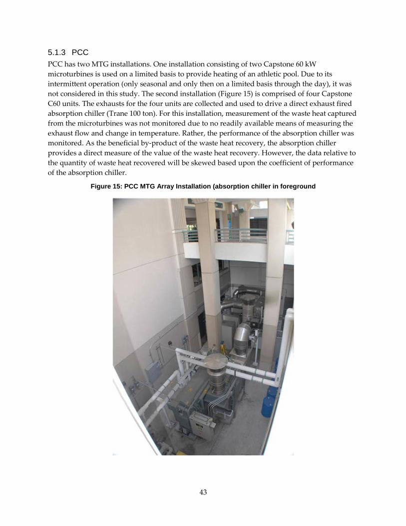
5.1.3 PCC PCC has two MTG installations. One installation consisting of two Capstone 60 kW microturbines is used on a limited basis to provide heating of an athletic pool. Due to its intermittent operation (only seasonal and only then on a limited basis through the day), it was not considered in this study. The second installation (Figure 15) is comprised of four Capstone C60 units. The exhausts for the four units are collected and used to drive a direct exhaust fired absorption chiller (Trane 100 ton). For this installation, measurement of the waste heat captured from the microturbines was not monitored due to no readily available means of measuring the exhaust flow and change in temperature. Rather, the performance of the absorption chiller was monitored. As the beneficial by-product of the waste heat recovery, the absorption chiller provides a direct measure of the value of the waste heat recovery. However, the data relative to the quantity of waste heat recovered will be skewed based upon the coefficient of performance of the absorption chiller.
Figure 15: PCC MTG Array Installation (absorption chiller in foreground
43
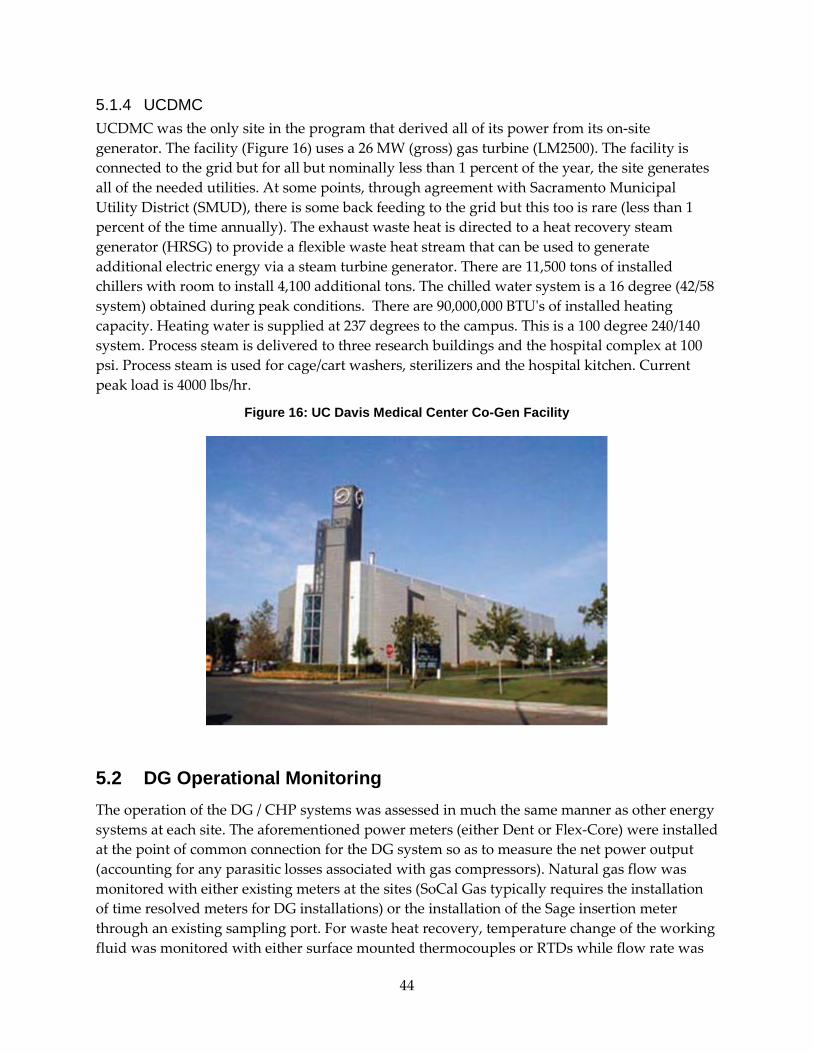
5.1.4 UCDMC UCDMC was the only site in the program that derived all of its power from its on-site generator. The facility (Figure 16) uses a 26 MW (gross) gas turbine (LM2500). The facility is connected to the grid but for all but nominally less than 1 percent of the year, the site generates all of the needed utilities. At some points, through agreement with Sacramento Municipal Utility District (SMUD), there is some back feeding to the grid but this too is rare (less than 1 percent of the time annually). The exhaust waste heat is directed to a heat recovery steam generator (HRSG) to provide a flexible waste heat stream that can be used to generate additional electric energy via a steam turbine generator. There are 11,500 tons of installed chillers with room to install 4,100 additional tons. The chilled water system is a 16 degree (42/58 system) obtained during peak conditions. There are 90,000,000 BTU's of installed heating capacity. Heating water is supplied at 237 degrees to the campus. This is a 100 degree 240/140 system. Process steam is delivered to three research buildings and the hospital complex at 100 psi. Process steam is used for cage/cart washers, sterilizers and the hospital kitchen. Current peak load is 4000 lbs/hr.
Figure 16: UC Davis Medical Center Co-Gen Facility
5.2 DG Operational Monitoring The operation of the DG / CHP systems was assessed in much the same manner as other energy systems at each site. The aforementioned power meters (either Dent or Flex-Core) were installed at the point of common connection for the DG system so as to measure the net power output (accounting for any parasitic losses associated with gas compressors). Natural gas flow was monitored with either existing meters at the sites (SoCal Gas typically requires the installation of time resolved meters for DG installations) or the installation of the Sage insertion meter through an existing sampling port. For waste heat recovery, temperature change of the working fluid was monitored with either surface mounted thermocouples or RTDs while flow rate was
44

monitored via the EMCO Sono-Trak meter and cross correlated/verified with logged operation of the pump motor and pump rating. For all aspects of the DG systems and sites monitored, there were no changes to the site plumbing to accommodate the measurement equipment. The non-intrusive nature of the measurement instruments not only resulted in expedited installations (no need for trades people to cut into pipe or install equipment), it was crucial in the agreement of site to permit the desired measurements.
Interestingly, two of the sites did not have thermal recovery instrumentation installed as part of the system (i.e. water flow meters, temperature sensors) while the other two did. The UCDMC, which utilizes its gas turbine and waste heat recovery for the entirety of the site’s energy need, had instrumentation in place and operational. Additionally, the CSUN molten carbonate fuel cell had a full complement of measurement equipment. However, the four microturbines at PCC and the two installations at AQMD headquarters did not have waste heat recovery instrumentation installed as part of the original equipment installation and site development.
For the three turbine system at AQMD, ITRON installed a set of instruments (ultrasonic flow meter and temperature sensors) for waste heat recovery as part of their role in the SGIP validation/verification program. The suggestion is that size of the system relative to the facility needs is paramount in determining both the level of instrumentation installed as well the funding and man-power necessary to maintain equipment.
In the following section, the results of the monitoring of the DG systems are presented. In reviewing the following graphs of efficiency for the sites, it is important to understand the basis upon which the values are calculated. The reported fuel to electric efficiency is based upon the lower heating value (LHV) of natural gas (approximately 910 btu/scf for Southern California).
This is the typical means of reporting prime generator efficiency and is the basis defined in the ASERTTI test protocolsError! Bookmark not defined.. However, when reporting the overall system thermal efficiency including waste heat recovery, the higher heating value of the natural gas is used (approximately 1020 btu/scf for Southern California) also as defined by the ASERTTI protocols. In general, “average” days for different quarters of a year (Jan-Mar = Winter, Apr- June = Spring, July – Sept = Summer, Oct-Dec= Fall) are presented with the net energy produced by the DG/CHP system for each 15 minute interval presented as “kw-hr” value. The power produced by the DG system is 4-times the energy value. The waste heat recovered was typically ascertained as the energy increase in the fluid (water) passing through the waste heat recovery heat exchangers based upon fluid flow rate, temperature rise, and fluid specific heat.
Exceptions to this are explained in the individual site sections below.
5.3 Utilization Results 5.3.1 AQMD Seasonal operational data for the AQMD installations are presented below in Figure 17through Figure 24. The installation comprised of four turbines (System 1) and net electric metering on each turbine whereas the installation comprised of three turbines (System 2) recorded the cumulative output for the array. For System 1, each turbine pair that fed one heat recovery unit
45

had the additional parasitic load of approximately 5 kW associated with the natural gas compressor the
(i.e., turbine #1 and turbine #3). For System 2, each turbine was connected to an individual compressor and as such, the individual turbine’s net output was reduced due to this parasitic load; since the cumulative net output was monitored, it was not possible to separate the individual turbine performance nor the parasitic loads associated with the compressors. In the graphs, System 1has each turbine listed individually while System 2 is listed as “3 MTG total”.
The systems have a nominal operational schedule of 8:00 am to 10:00 or 11:00 pm (depending upon the system and the time of year) Monday – Friday, no operation on Saturday or Sunday. The plots shown in the figures do not discern between weekend and week days; hence, on average there would be an expected reduction of the average energy output of 28.6 percent (2/7th of the week). For a nominal rated 60 kW turbine (as is the case for the 4-MTG installation), the expected gross maximum energy during operation would be:
60/4 x (1-.286) = 10.7 kW-hr
For the three 65-kW microturbine system, a similar calculation of the maximum gross output is:
(65*3)/4 * (1-.286) = 34.8 kW-hr
Figure 17: AQMD MTG Installation: Typical Energy Profile: Oct-Dec 2008
46
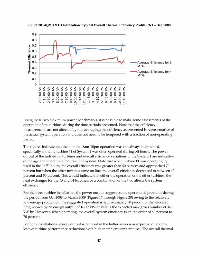
Figure 18: AQMD MTG Installation: Typical Overall Thermal Efficiency Profile: Oct – Dec 2008
Using these two maximum power benchmarks, it is possible to make some assessments of the operation of the turbines during the time periods presented. Note that the efficiency measurements are not affected by this averaging; the efficiency as presented is representative of the actual system operation and does not need to be tempered with a fraction of non-operating period.
The figures indicate that the nominal 8am-10pm operation was not always maintained, specifically showing turbine #1 of System 1 was often operated during off hours. The power output of the individual turbines and overall efficiency variations of the System 1 are indicative of the age and operational hours of the system. Note that when turbine #1 was operating by itself in the “off” hours, the overall efficiency was greater than 50 percent and approached 70 percent but when the other turbines came on line, the overall efficiency decreased to between 40 percent and 50 percent. This would indicate that either the operation of the other turbines, the heat exchanger for the #3 and #4 turbines, or a combination of the two affects the system efficiency.
For the three turbine installation, the power output suggests some operational problems during the period from Oct 2008 to March 2009 (Figure 17 through Figure 20) owing to the relatively low energy production; the suggested operation is approximately 50 percent of the allocated time, shown by an energy output of 16-17 kW-hr versus the expected max gross number of 34.8 kW-hr. However, when operating, the overall system efficiency is on the order of 50 percent to 70 percent.
For both installations, energy output is reduced in the hotter seasons as expected due to the known turbine performance reductions with higher ambient temperatures. The overall thermal
0
0.1
0.2
0.3
0.4
0.5
0.6
0.7
0.8
0.9
12:0
0:00
AM
1:15
:00
AM
2:30
:00
AM
3:45
:00
AM
5:00
:00
AM
6:15
:00
AM
7:30
:00
AM
8:45
:00
AM
10:0
0:00
AM
11:1
5:00
AM
12:3
0:00
PM
1:45
:00
PM
3:00
:00
PM
4:15
:00
PM
5:30
:00
PM
6:45
:00
PM
8:00
:00
PM
9:15
:00
PM
10:3
0:00
PM
11:4
5:00
PM
Ther
mal
Effi
cien
cy
Average Efficiency for 3MTG
Average Efficiency for 4MTG
47
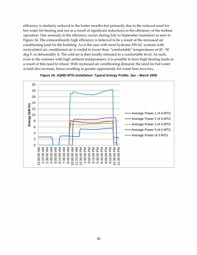
efficiency is similarly reduced in the hotter months but primarily due to the reduced need for hot water for heating and not as a result of significant reductions in the efficiency of the turbine operation. One anomaly in the efficiency occurs during July to September (summer) as seen in Figure 24. The extraordinarily high efficiency is believed to be a result of the increased air conditioning load for the building. As is the case with most hydronic HVAC systems with recirculated air, conditioned air is cooled to lower than “comfortable” temperatures of 45 - 50 deg F, to dehumidify it. The cold air is then locally reheated to a comfortable level. As such, even in the summer with high ambient temperatures, it is possible to have high heating loads as a result of this need to reheat. With increased air conditioning demand, the need for hot water would also increase, hence resulting in greater opportunity for waste heat recovery.
Figure 19: AQMD MTG Installation: Typical Energy Profile: Jan – March 2009
0
2
4
6
8
10
12
14
16
18
20
12:0
0:00
AM
1:15
:00
AM
2:30
:00
AM
3:45
:00
AM
5:00
:00
AM
6:15
:00
AM
7:30
:00
AM
8:45
:00
AM
10:0
0:00
AM
11:1
5:00
AM
12:3
0:00
PM
1:45
:00
PM
3:00
:00
PM
4:15
:00
PM
5:30
:00
PM
6:45
:00
PM
8:00
:00
PM
9:15
:00
PM
10:3
0:00
PM
11:4
5:00
PM
Ener
gy (k
W-h
r)
Average Power 1 of 4 MTG
Average Power 2 of 4 MTG
Average Power 3 of 4 MTG
Average Power 4 of 4 MTG
Average Power of 3 MTG
48
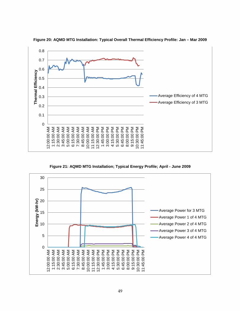
Figure 20: AQMD MTG Installation: Typical Overall Thermal Efficiency Profile: Jan – Mar 2009
Figure 21: AQMD MTG Installation; Typical Energy Profile; April - June 2009
0
0.1
0.2
0.3
0.4
0.5
0.6
0.7
0.812
:00:
00 A
M1:
15:0
0 A
M2:
30:0
0 A
M3:
45:0
0 A
M5:
00:0
0 A
M6:
15:0
0 A
M7:
30:0
0 A
M8:
45:0
0 A
M10
:00:
00 A
M11
:15:
00 A
M12
:30:
00 P
M1:
45:0
0 P
M3:
00:0
0 P
M4:
15:0
0 P
M5:
30:0
0 P
M6:
45:0
0 P
M8:
00:0
0 P
M9:
15:0
0 P
M10
:30:
00 P
M11
:45:
00 P
M
The
rmal
Effi
cien
cy
Average Efficiency of 4 MTG
Average Efficiency of 3 MTG
0
5
10
15
20
25
30
12:0
0:00
AM
1:15
:00
AM
2:30
:00
AM
3:45
:00
AM
5:00
:00
AM
6:15
:00
AM
7:30
:00
AM
8:45
:00
AM
10:0
0:00
AM
11:1
5:00
AM
12:3
0:00
PM
1:45
:00
PM
3:00
:00
PM
4:15
:00
PM
5:30
:00
PM
6:45
:00
PM
8:00
:00
PM
9:15
:00
PM
10:3
0:00
PM
11:4
5:00
PM
Ener
gy (k
W-h
r)
Average Power for 3 MTG
Average Power 1 of 4 MTG
Average Power 2 of 4 MTG
Average Power 3 of 4 MTG
Average Power 4 of 4 MTG
49

Figure 22: AQMD MTG Installation: Typical Overall Thermal Efficiency; April - June 2009
Figure 23: AQMD MTG Installation: Typical Energy Profile; July - Sept 2009
0
0.1
0.2
0.3
0.4
0.5
0.6
0.7
12:0
0:00
AM
1:15
:00
AM
2:30
:00
AM
3:45
:00
AM
5:00
:00
AM
6:15
:00
AM
7:30
:00
AM
8:45
:00
AM
10:0
0:00
AM
11:1
5:00
AM
12:3
0:00
PM
1:45
:00
PM
3:00
:00
PM
4:15
:00
PM
5:30
:00
PM
6:45
:00
PM
8:00
:00
PM
9:15
:00
PM
10:3
0:00
PM
11:4
5:00
PM
The
rmal
Effi
cien
cy
Average Efficiency for 3MTG
Average Efficiency for 4MTG
0
5
10
15
20
25
01:
00:0
0 A
M2:
15:0
0 A
M3:
30:0
0 A
M4:
45:0
0 A
M6:
00:0
0 A
M7:
15:0
0 A
M8:
30:0
0 A
M9:
45:0
0 A
M11
:00:
00 A
M12
:15:
00 P
M1:
30:0
0 P
M2:
45:0
0 P
M4:
00:0
0 P
M5:
15:0
0 P
M6:
30:0
0 P
M7:
45:0
0 P
M9:
00:0
0 P
M10
:15:
00 P
M11
:30:
00 P
M
Ener
gy (k
W-h
r)
Average Power for 3 MTG
Average Power 1 of 4 MTG
Average Power 2 of 4 MTG
Average Power 3 of 4 MTG
Average Power 4 of 4 MTG
50
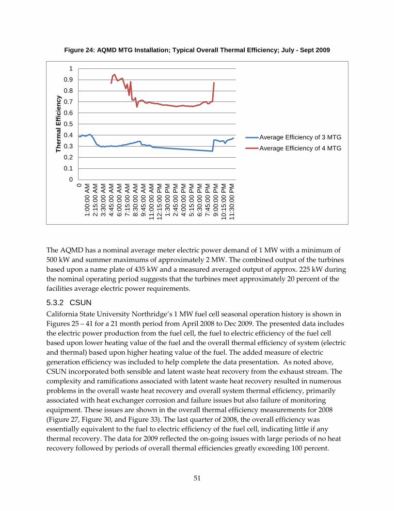
Figure 24: AQMD MTG Installation; Typical Overall Thermal Efficiency; July - Sept 2009
The AQMD has a nominal average meter electric power demand of 1 MW with a minimum of 500 kW and summer maximums of approximately 2 MW. The combined output of the turbines based upon a name plate of 435 kW and a measured averaged output of approx. 225 kW during the nominal operating period suggests that the turbines meet approximately 20 percent of the facilities average electric power requirements.
5.3.2 CSUN California State University Northridge’s 1 MW fuel cell seasonal operation history is shown in Figures 25 – 41 for a 21 month period from April 2008 to Dec 2009. The presented data includes the electric power production from the fuel cell, the fuel to electric efficiency of the fuel cell based upon lower heating value of the fuel and the overall thermal efficiency of system (electric and thermal) based upon higher heating value of the fuel. The added measure of electric generation efficiency was included to help complete the data presentation. As noted above, CSUN incorporated both sensible and latent waste heat recovery from the exhaust stream. The complexity and ramifications associated with latent waste heat recovery resulted in numerous problems in the overall waste heat recovery and overall system thermal efficiency, primarily associated with heat exchanger corrosion and failure issues but also failure of monitoring equipment. These issues are shown in the overall thermal efficiency measurements for 2008 (Figure 27, Figure 30, and Figure 33). The last quarter of 2008, the overall efficiency was essentially equivalent to the fuel to electric efficiency of the fuel cell, indicating little if any thermal recovery. The data for 2009 reflected the on-going issues with large periods of no heat recovery followed by periods of overall thermal efficiencies greatly exceeding 100 percent.
0
0.1
0.2
0.3
0.4
0.5
0.6
0.7
0.8
0.9
10
1:00
:00
AM
2:15
:00
AM
3:30
:00
AM
4:45
:00
AM
6:00
:00
AM
7:15
:00
AM
8:30
:00
AM
9:45
:00
AM
11:0
0:00
AM
12:1
5:00
PM
1:30
:00
PM
2:45
:00
PM
4:00
:00
PM
5:15
:00
PM
6:30
:00
PM
7:45
:00
PM
9:00
:00
PM
10:1
5:00
PM
11:3
0:00
PM
Ther
mal
Effi
cien
cy
Average Efficiency of 3 MTG
Average Efficiency of 4 MTG
51
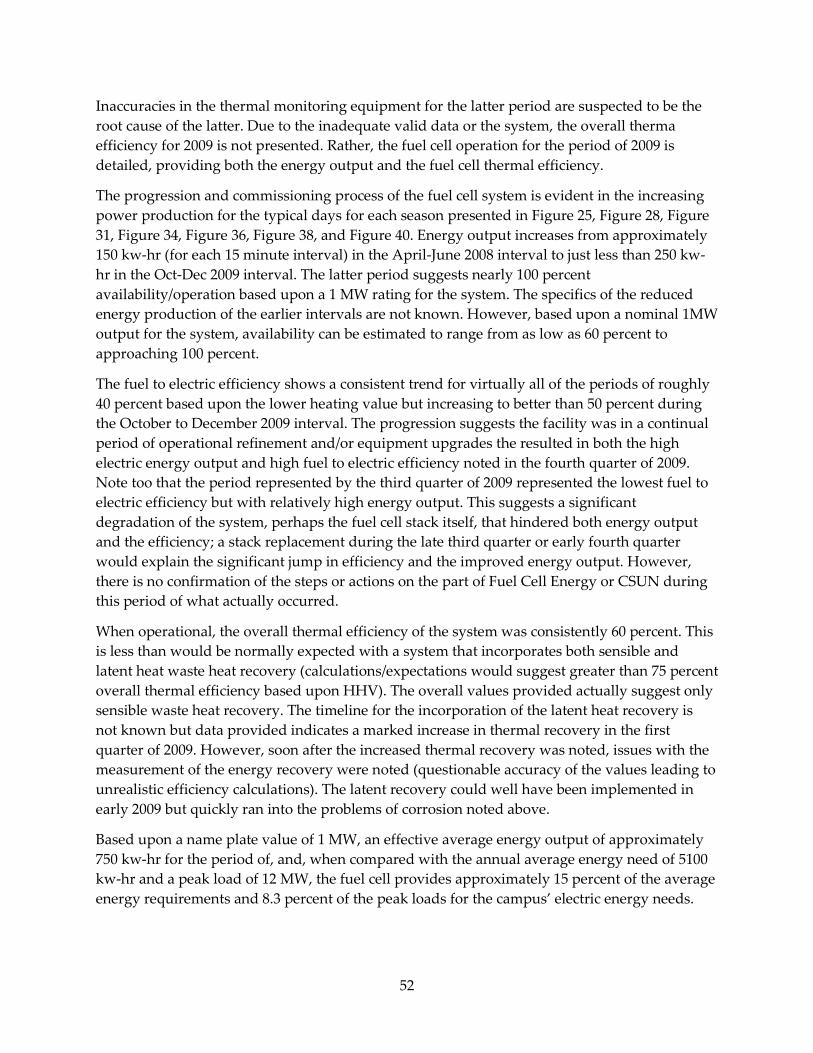
Inaccuracies in the thermal monitoring equipment for the latter period are suspected to be the root cause of the latter. Due to the inadequate valid data or the system, the overall therma efficiency for 2009 is not presented. Rather, the fuel cell operation for the period of 2009 is detailed, providing both the energy output and the fuel cell thermal efficiency.
The progression and commissioning process of the fuel cell system is evident in the increasing power production for the typical days for each season presented in Figure 25, Figure 28, Figure 31, Figure 34, Figure 36, Figure 38, and Figure 40. Energy output increases from approximately 150 kw-hr (for each 15 minute interval) in the April-June 2008 interval to just less than 250 kw- hr in the Oct-Dec 2009 interval. The latter period suggests nearly 100 percent availability/operation based upon a 1 MW rating for the system. The specifics of the reduced energy production of the earlier intervals are not known. However, based upon a nominal 1MW output for the system, availability can be estimated to range from as low as 60 percent to approaching 100 percent.
The fuel to electric efficiency shows a consistent trend for virtually all of the periods of roughly 40 percent based upon the lower heating value but increasing to better than 50 percent during the October to December 2009 interval. The progression suggests the facility was in a continual period of operational refinement and/or equipment upgrades the resulted in both the high electric energy output and high fuel to electric efficiency noted in the fourth quarter of 2009. Note too that the period represented by the third quarter of 2009 represented the lowest fuel to electric efficiency but with relatively high energy output. This suggests a significant degradation of the system, perhaps the fuel cell stack itself, that hindered both energy output and the efficiency; a stack replacement during the late third quarter or early fourth quarter would explain the significant jump in efficiency and the improved energy output. However, there is no confirmation of the steps or actions on the part of Fuel Cell Energy or CSUN during this period of what actually occurred.
When operational, the overall thermal efficiency of the system was consistently 60 percent. This is less than would be normally expected with a system that incorporates both sensible and latent heat waste heat recovery (calculations/expectations would suggest greater than 75 percent overall thermal efficiency based upon HHV). The overall values provided actually suggest only sensible waste heat recovery. The timeline for the incorporation of the latent heat recovery is not known but data provided indicates a marked increase in thermal recovery in the first quarter of 2009. However, soon after the increased thermal recovery was noted, issues with the measurement of the energy recovery were noted (questionable accuracy of the values leading to unrealistic efficiency calculations). The latent recovery could well have been implemented in early 2009 but quickly ran into the problems of corrosion noted above.
Based upon a name plate value of 1 MW, an effective average energy output of approximately 750 kw-hr for the period of, and, when compared with the annual average energy need of 5100 kw-hr and a peak load of 12 MW, the fuel cell provides approximately 15 percent of the average energy requirements and 8.3 percent of the peak loads for the campus’ electric energy needs.
52
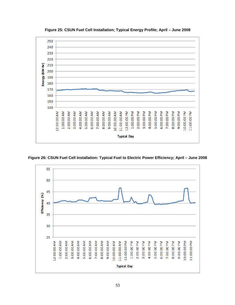
Figure 25: CSUN Fuel Cell Installation; Typical Energy Profile; April – June 2008
Figure 26: CSUN Fuel Cell Installation: Typical Fuel to Electric Power Efficiency; April – June 2008
53
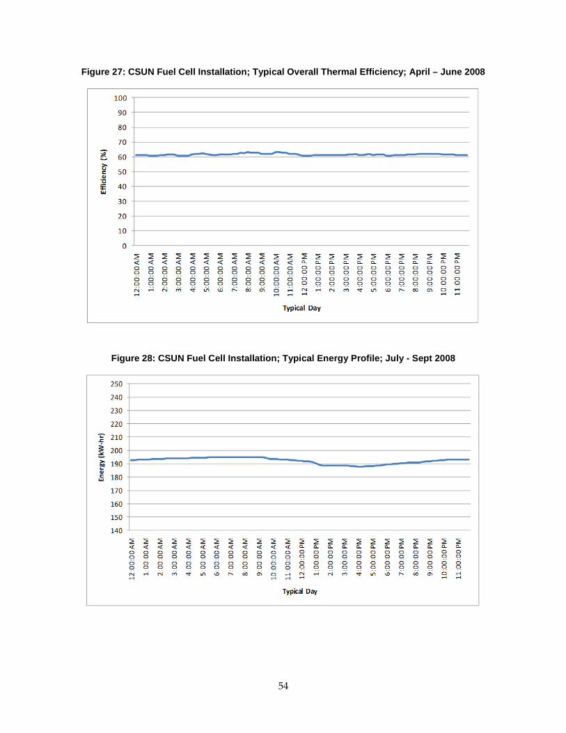
Figure 27: CSUN Fuel Cell Installation; Typical Overall Thermal Efficiency; April – June 2008
Figure 28: CSUN Fuel Cell Installation; Typical Energy Profile; July - Sept 2008
54

Figure 29: CSUN Fuel Cell Installation: Typical Fuel to Electric Power Efficiency; April – June 2008
Figure 30: CSUN Fuel Cell Installation; Typical Overall Thermal Efficiency; July - Sept 2008
55
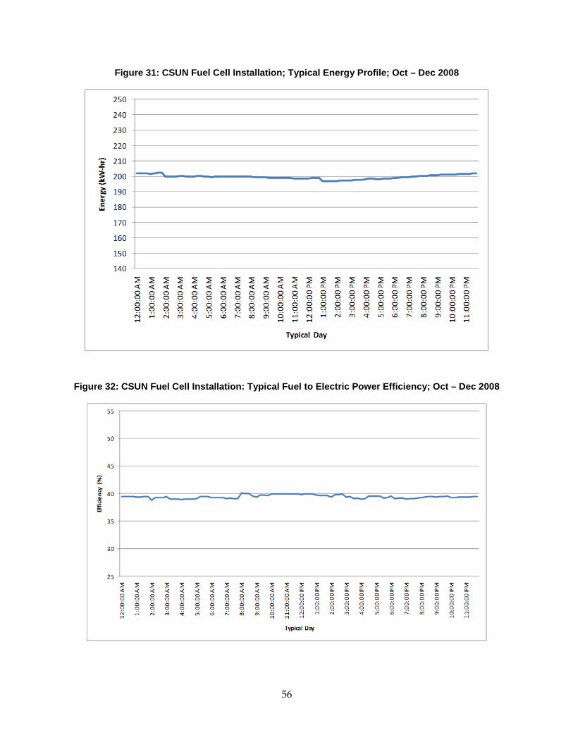
Figure 31: CSUN Fuel Cell Installation; Typical Energy Profile; Oct – Dec 2008
Figure 32: CSUN Fuel Cell Installation: Typical Fuel to Electric Power Efficiency; Oct – Dec 2008
56

Figure 33: CSUN Fuel Cell Installation; Typical Overall Thermal Efficiency; Oct – Dec 2008
Figure 34: CSUN Fuel Cell Installation; Typical Energy Profile; Jan – March 2009
57
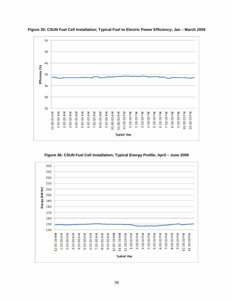
Figure 35: CSUN Fuel Cell Installation; Typical Fuel to Electric Power Efficiency; Jan – March 2009
Figure 36: CSUN Fuel Cell Installation; Typical Energy Profile; April – June 2009
58

Figure 37: CSUN Fuel Cell Installation; Typical Fuel to Electric Power Efficiency; April – June 2009
Figure 38: CSUN Fuel Cell Installation; Typical Energy Profile; July – Sept 2009
59

Figure 39: CSUN Fuel Cell Installation; Typical Fuel to Electric Power Efficiency; July – Sept 2009
Figure 40: CSUN Fuel Cell Installation; Typical Energy Profile; Oct – Dec 2009
60
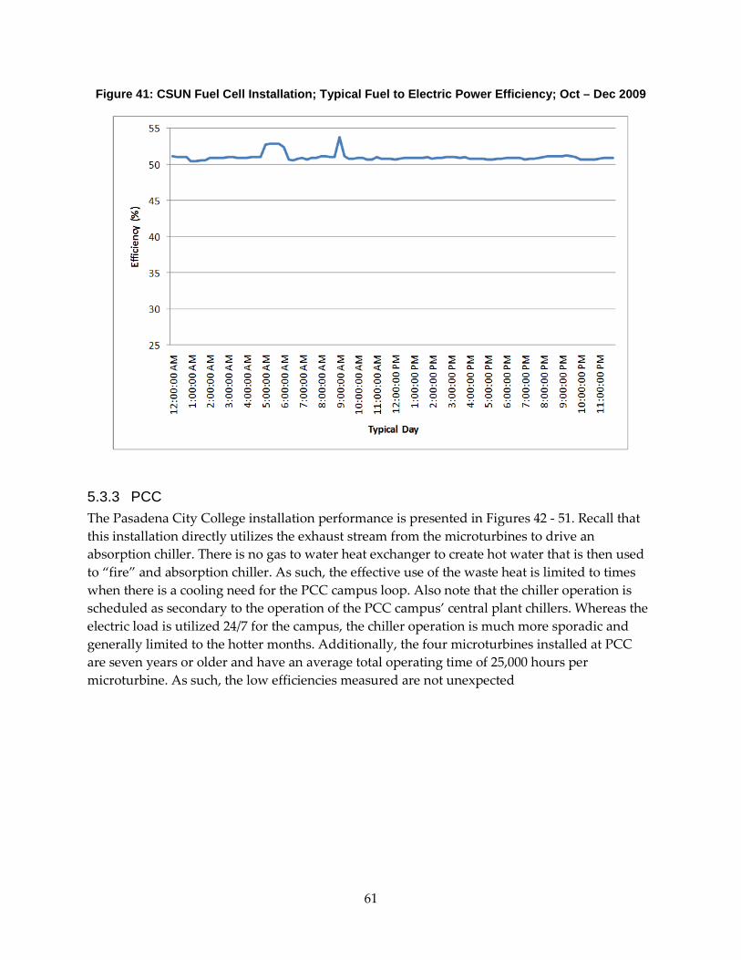
Figure 41: CSUN Fuel Cell Installation; Typical Fuel to Electric Power Efficiency; Oct – Dec 2009
5.3.3 PCC The Pasadena City College installation performance is presented in Figures 42 - 51. Recall that this installation directly utilizes the exhaust stream from the microturbines to drive an absorption chiller. There is no gas to water heat exchanger to create hot water that is then used to “fire” and absorption chiller. As such, the effective use of the waste heat is limited to times when there is a cooling need for the PCC campus loop. Also note that the chiller operation is scheduled as secondary to the operation of the PCC campus’ central plant chillers. Whereas the electric load is utilized 24/7 for the campus, the chiller operation is much more sporadic and generally limited to the hotter months. Additionally, the four microturbines installed at PCC are seven years or older and have an average total operating time of 25,000 hours per microturbine. As such, the low efficiencies measured are not unexpected
61

Figure 42: PCC MTG / Chiller Array; Typical Electric Energy Output; Sept-Dec 2008
Figure 43: PCC MTG / Chiller Array; Typical Overall System Efficiency; Sept – Dec 2008
62

Figure 44: PCC MTG / Chiller Array; Typical Electric Energy Output; Jan – Mar 2009
Figure 45: PCC MTG / Chiller Array; Typical Overall System Efficiency; Jan-Mar 2009
63
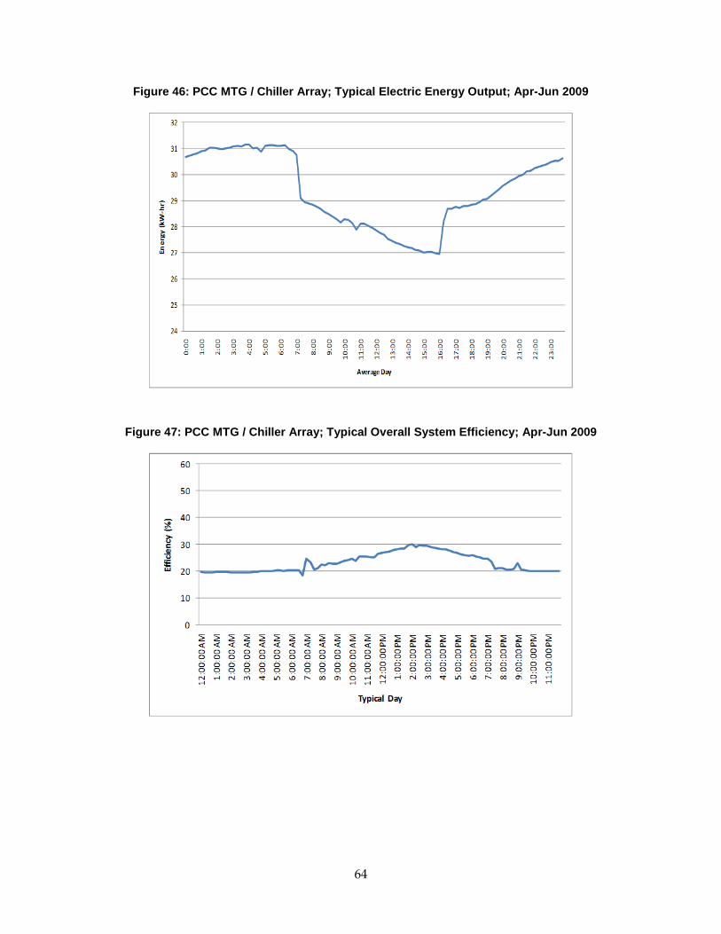
Figure 46: PCC MTG / Chiller Array; Typical Electric Energy Output; Apr-Jun 2009
Figure 47: PCC MTG / Chiller Array; Typical Overall System Efficiency; Apr-Jun 2009
64

Figure 48: PCC MTG / Chiller Array; Typical Electric Energy Output; Jul-Sept 2009
Figure 49: PCC MTG / Chiller Array; Typical Overall System Efficiency; Jul-Sept 2009
65
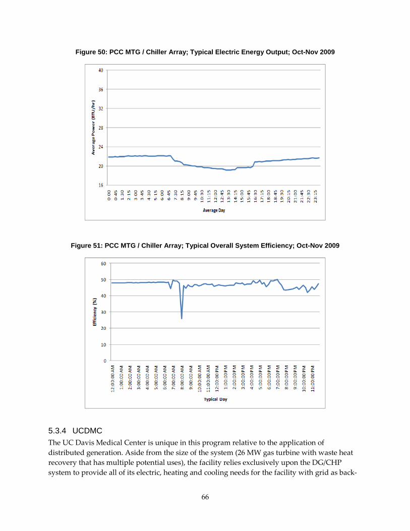
Figure 50: PCC MTG / Chiller Array; Typical Electric Energy Output; Oct-Nov 2009
Figure 51: PCC MTG / Chiller Array; Typical Overall System Efficiency; Oct-Nov 2009
5.3.4 UCDMC The UC Davis Medical Center is unique in this program relative to the application of distributed generation. Aside from the size of the system (26 MW gas turbine with waste heat recovery that has multiple potential uses), the facility relies exclusively upon the DG/CHP system to provide all of its electric, heating and cooling needs for the facility with grid as back-
66

up. As such, the presented information in Figure 52– Figure 59 do not provide the energy production of the turbine or the system since this is nominally equivalent to and would be representative of the facility loads, not the capability of the DG system to meet the load. Rather, the figures present the fuel to electric efficiency of the gas turbine and the overall thermal efficiency. As with the other cases presented, the overall efficiency is presented in term of higher heating value of the fuel (1020 btu/scf). For the fuel to electric efficiency, the results are presented in terms of the lower heating value of the fuel, consistent with the ASERTTI16distributed generation testing protocols.
For the 12 month period presented in Figures 52 - 59, the general trend is similar. That is, overnight electrical generation efficiency of approximately 28 percent due to the turbine operating at reduced load consistent with the facility demands at night (typically less than 10 MW as compared to the 26 MW rating of the turbine); overall thermal efficiency overnight is approximately 58 percent. As the loads come on line with the normal business hours, the turbine efficiency increases to between 31 percent and 32 percent, associated with the increased load demand moving more towards the full load; overall thermal efficiency increases to greater than 60 percent, peaking at 64 percent. Throughout the year, the peak in efficiency for both the turbine and the overall facility seems to occur between 4 and 6 pm, ostensibly the time when the load for facility electric power and air conditioning would be largest.
What is not represented by these values is the flexibility of the waste heat recovery in meeting the other demands of the facility. Recall that the waste heat recovered in the heat recovery steam generator (HRSG) can be directed as needed to many applications, either operating alone or in combination absorption chillers, hot water, and auxiliary electric power production. The overall thermal efficiency is based upon the waste heat recovered in the HRSG and not representative of the final use of the energy (i.e. the final “product”).
In its role as the primary electric and thermal energy source for the Medical Center, the system operated with a very high capacity factor. All of the outages during the monitoring period were scheduled representing normal preventative maintenance and as well as two periods dedicated to major but planned outages for service. Regular maintenance was generally scheduled for Tuesdays or Thursday on nominally 2 month intervals. Outages were nominally 12 hours long from 5 am to approximately 5 pm for a total of 56 ½ hours for the period. Interestingly no attempt was made to shift the timing to “off-peak” hours but this may be a function of details of the agreement the facility has with the local utility (SMUD). The longer outages occurred in December 2008 (3-days) and March 2009 (4 days) for a total of 176 ¾ hours. These represent a total capacity factor of approximately 97.3 percent for the 12 months of monitoring; the regular service representing 0.65 percent of the full year and the extended service representing 2 percent of the full year
16 Association of State Energy Research and Technology Transfer Institutions; 455 Science Dr, Ste 200, Madison WI, 53711
67
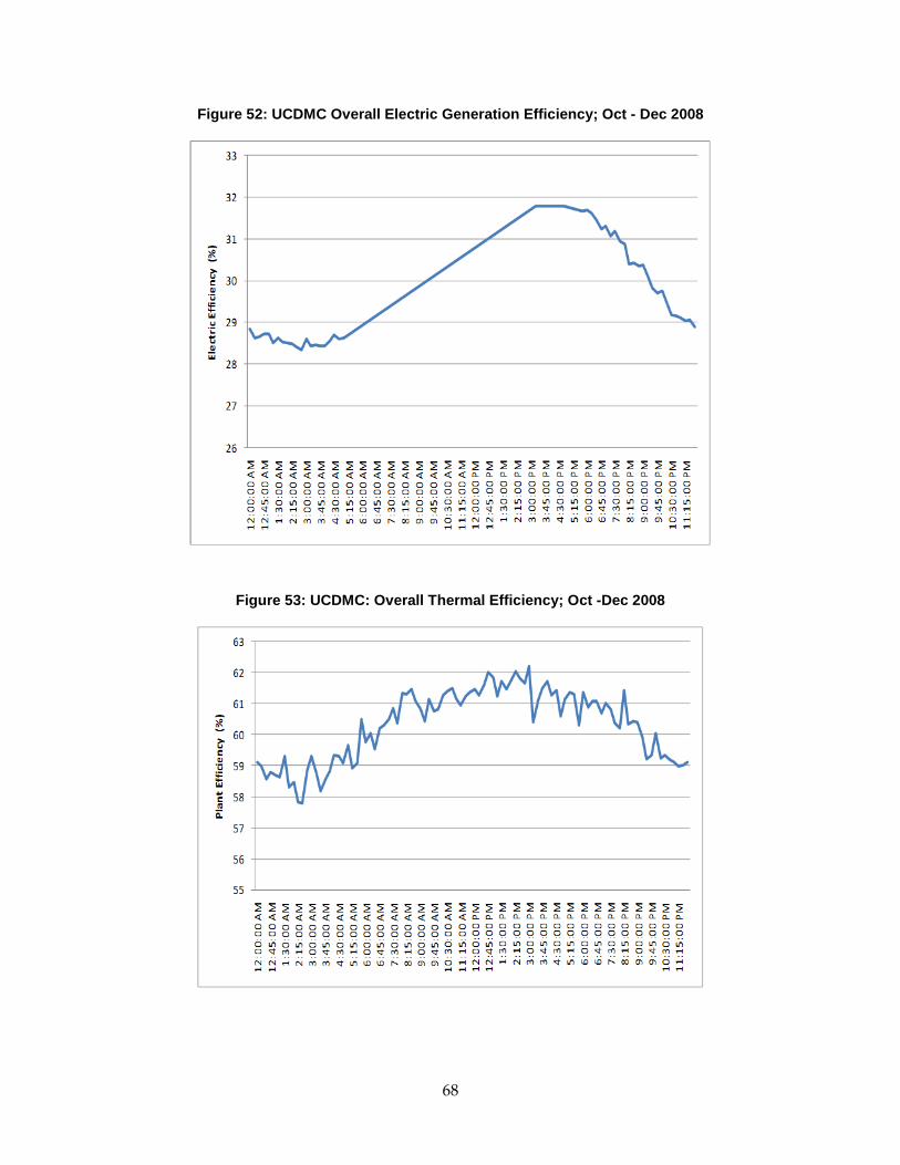
Figure 52: UCDMC Overall Electric Generation Efficiency; Oct - Dec 2008
Figure 53: UCDMC: Overall Thermal Efficiency; Oct -Dec 2008
68

Figure 54: UCDMC: Overall Electric Generation Efficiency; Jan - Mar 2009
Figure 55: UCDMC Overall Thermal Efficiency; Jan - Mar 2009
69
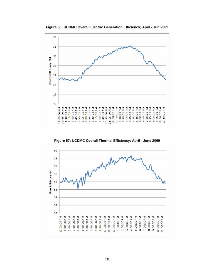
Figure 56: UCDMC Overall Electric Generation Efficiency; April - Jun 2009
Figure 57: UCDMC Overall Thermal Efficiency; April - June 2009
70
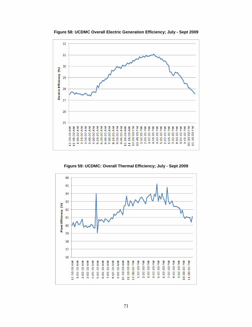
Figure 58: UCDMC Overall Electric Generation Efficiency; July - Sept 2009
Figure 59: UCDMC: Overall Thermal Efficiency; July - Sept 2009
71
5.4 Observations Regarding DG/CHP Utilization The preceding examples, while small in number, could be considered representative of the general application and success of distributed generation. All are providing facility support in the form of both electric power and thermal support and provide a snapshot of the level of success for the application of DG/CHP in facilities.
The facilities represent three of the six sectors investigated in this program: college/university, commercial office, and hospital. They also essentially represent three different distributed generation prime movers: microturbines, gas turbines, and fuel cells.
The Central Plant nature of the UC Davis Medical Center and the critical support it provides for the facility operation is evident in the exceptional availability of the system during the period of monitoring during this program. The system inherently warrants high levels of system support from the facilities group at the UCDMC, certainly a consideration during the system’s initial design and deployment. The fuel to electric efficiency measured is consistent with the expectations of a gas turbine engine of the size and vintage installed. The overall efficiency is perhaps lower than what would be expected; however, note that the engine is greatly oversized for the facility (26 MW rating versus nominal hospital loads of 15-18 MW) with room for future expansion. The same argument can be made for the waste heat recovery in that the site loads are currently less than the capacity of the system. Hence, some waste heat must be bypassed leading to reduced overall thermal efficiency. However, this site does well represent the potential of DG/CHP for exceptional efficiencies when designed to meet the entire load profile for a site.
The history of the CSUN fuel cell installation as documented in the monitored data is one of continual refinement as well as the issues associated with trying to maximize the waste heat recovery. The improvement of energy output and overall efficiency are testament to the on- going efforts of the staff at CSUN. The data for the period of Oct – Dec 2009 are representative of the expected fuel cell operation owing to both continual system refinement as well as a likely stack replacement. Unfortunately, the waste heat recovery data is somewhat more erratic owing to system issues with the latent heat recovery from the exhaust. However for small segments of data that are deemed accurate, overall efficiencies of more than 85 percent have been measured. While large amounts of waste heat capture are possible with latent heat recovery, its application in general DG/CHP applications must be carefully weighed against the added maintenance necessary due to the corrosive environment and the quality of the heat recovered relative to the application.
PCC has an array of four older, high operational hours, C-60 turbines with direct waste heat recovery to an absorption chiller. While an admirable system that should have provided exceptional operational efficiency, the overall system efficiency suffered from both the age of the turbines and numerous operational problems with the chiller. Further, the age of the turbines complicates the continued service since Capstone does not support some of the key components of the system as is but requires upgrades.
72

SCAQMD, like PCC has an array of four older turbines that suffer from the same reductions in power output, efficiency, and serviceability as the PCC system. However, the waste heat recovery in the form of hot water to augment the on-site boilers does result in better overall efficiencies due to higher availability. The simplicity of the system certainly helps in this regard with a simple heat exchanger and pump as opposed to the complexity of an absorption chiller system with multiple possible points of failure. The second, three turbine array at AQMD extends the same system design with upgrades to the heat exchangers that have been identified over the years. The age and improved waste heat recovery result in increased output and efficiencies than the older array. One system design of concern at both AQMD installations is the distance between the waste heat capture points and the point of connection with the building heating loop. The program did not measure the temperatures at the point of connection but rather at the heat exchangers. The energy loss and parasitic pumping loads associated with the waste heat recovery were not quantified but are suspected to be significant
73

CHAPTER 6: Relative Exposure Analysis The effects of widespread deployment of DG/CHP systems on the air shed are currently unknown. Generally, the expectations of higher overall thermal efficiency would result in reductions in the emissions of greenhouse gases (primarily carbon dioxide). Additionally, current DG/CHP systems eligible for simplified deployment throughout California are required to meet stringent emission levels comparable to central station stationary source BACT levels but with the added caveat that 100 percent credit is given for all waste heat energy that is recovered and is added to the electric energy provided to establish the denominator for the emissions rate calculations (i.e. emission in “lb/MW-hr” inclusive of electric and waste energy).
An assessment of the ramifications of widespread deployment of DG/CHP is addressed in this task. The evaluation undertaken herein is at two distinct and diverse scales. The first assessment evaluates the impacts on an air shed level (e.g. the South Coast Air Basin) relative to particulate and ozone level while the second evaluates the effect of the emissions on the near field adjacent to the DG system ambient air quality relative to standard for criteria pollutants.
6.1 Air Quality Impacts Modeling 6.1.1 Summary This report analyzes the potential air quality impacts of using DG/CHP applications to supply electrical and thermal needs to food retail stores in the South Coast Air Basin of California (SoCAB). The use of CHP would displace power supply from the grid that otherwise would be required for the food retail sector.
The program limitations did not permit air quality impacts modeling/analysis of all of the sectors monitored. Based upon the potential for excellent waste heat utilization, the 24/7 nature of its operation, the number of locations in the SoCAB, and the general proximity to residential areas where near field air quality impacts may be most prevalent, the food/grocery sector was selected for the air quality impacts modeling Based on estimates by the California Energy Commission, the food retail industry consumed 4401 GWh in the year 2007, 3.6 percent of total consumption in the basin. This level of consumption is equivalent to an average power capacity of 500 MW. Hence, the use of CHP in food/retail buildings in the SoCAB could replace one average-sized power plant.
6.1.2 Spatial Distribution of Distributed Generation for Retail Stores Figure 60 and Figure 61depict the spatial information that is available to allocate on-site distributed power generation for food retail stores. The image corresponds to a subset of Geographical Information Systems (GIS) land use data for the SoCAB. GIS land use data includes spatial information of four different categories of retail activities:
• Regional shopping centers: this category includes large retail malls such as the South Coast Plaza, Fashion Island and the Irvine Spectrum. Typically, these areas do not include large food retail stores.
74

• Retail centers: this category includes a mix of food retail stores (e.g. Albertson’s, Vons) with general retail stores that also serve food products (e.g. Target, Costco). In addition, these areas include restaurants.
• Modern strip development: these areas include mostly restaurants, bars and convenience stores.
• Older strip development: as in modern strip development, these areas include mostly restaurants, bars and convenience stores.
The purpose of this study is to analyze the potential air quality impact of using distributed generation (DG) in large food retail stores. Retail centers category (category 2) is the GIS land use type that includes most food retail stores. Consequently, that category is used to spatially allocate DG installations in the SoCAB. Figure 62 (a) presents the spatial distribution of retail center area in the SoCAB. There is a high percentage of area ( about 1 percent) in the retail store category north of Riverside (in the Riverside County) and south of Anaheim (in the Orange County), whereas in central Los Angeles the area designated for retail stores is less than 0.2 percent.
Regarding energy use for food refrigeration, one would expect to find the peak demand around areas with the highest population density, such as central Los Angeles. However, GIS land use data does not correlate directly with population density, shown in Figure 62(b). GIS land use data only provides information on the ground level area of the retail store. It does not include information of whether stores include multiple floors and it does not provide information on sales volumes, which can affect the total energy load required for food retail stores. As a result, using information in Figure 62(a) alone as a spatial surrogate for distribution of DG would bias DG deployment towards Riverside. To correct this bias, the spatial distribution of DG is the normalized product of retail store area multiplied by the population density. The resulting spatial distribution is presented in Figure 62(c).
75

Figure 60: GIS land use data of spatial distribution of retail centers in the South Coast Air Basin
76

Figure 61: Insert of Figure 60 Showing GIS Land Use Data of Spatial Distribution of Retail Centers in and Around the Newport Beach Area
77
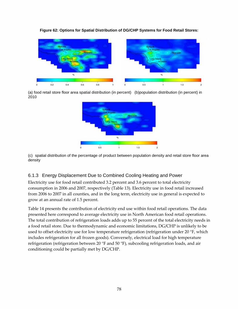
Figure 62: Options for Spatial Distribution of DG/CHP Systems for Food Retail Stores:
(a) food retail store floor area spatial distribution (in percent) (b)population distribution (in percent) in 2010
(c) spatial distribution of the percentage of product between population density and retail store floor area density
6.1.3 Energy Displacement Due to Combined Cooling Heating and Power Electricity use for food retail contributed 3.2 percent and 3.6 percent to total electricity consumption in 2006 and 2007, respectively (Table 13). Electricity use in food retail increased from 2006 to 2007 in all counties, and in the long term, electricity use in general is expected to grow at an annual rate of 1.5 percent.
Table 14 presents the contribution of electricity end use within food retail operations. The data presented here correspond to average electricity use in North American food retail operations. The total contribution of refrigeration loads adds up to 55 percent of the total electricity needs in a food retail store. Due to thermodynamic and economic limitations, DG/CHP is unlikely to be used to offset electricity use for low temperature refrigeration (refrigeration under 20 °F, which includes refrigeration for all frozen goods). Conversely, electrical load for high temperature refrigeration (refrigeration between 20 °F and 50 °F), subcooling refrigeration loads, and air conditioning could be partially met by DG/CHP.
78

Table 13: Electricity Consumption in Food Retail and Related Activities by County (from the energy consumption data management system, California Energy Commission
Electricity Consumption - Year 2006
County Food retail* Total Food retail contribution
(Million kWh) (Million kWh) (%)
Los Angeles 2279 70662 3.2
Orange 704 21145 3.3
Riverside 422 14840 2.8
San Bernardino 453 14594 3.1
Total 3858 121241 3.2
Electricity Consumption - Year 2007
County Food retail Total Food retail contribution
(Million kWh) (Million kWh) (%)
Los Angeles 2519 69666 3.6
Orange 920 21905 4.2
Riverside 476 14645 3.2
San Bernardino 487 15505 3.1
Total 4401 121720 3.6
*Food retail encompasses grocery, food and beverages stores, categories included in the North American Industrial Classification System (NAICS)
79

Table 14: Distribution of Electricity Needs by End Use in Food Retail Stores (ASHRAE, 2008)
End use %
Refrigeration needs:
Low temperature refrigeration a 12
High temperature refrigeration b 38
Heating, ventilating and air conditioning 5
Other needs:
Lighting 38
Food preparation 7
a Low Temperature Refrigeration: refrigeration under 20 oF b High Temperature Refrigeration: refrigeration above 20 oF and under 50 oF, which includes subcooling refrigeration loads
Figure 63 through Figure 66 show four possible CHP configurations as an alternative to conventional “grid connected” electricity use in food retail stores wherein all the electricity and thermal loads are supplied by electricity from the grid. The four DG/CHP cases assume that the DG/CHP is self-sufficient, and does not require additional electricity from the grid. The four cases presented in figures below are the following:
1. Internal Combustion Engine (ICE) prime mover; HVAC load priority for CHP (Figure 63): the DG/CHP system provides all the electrical needs, and the excess heat is used in an absorption chiller to provide the cooling needs for HVAC. Since HVAC loads are a small portion of the total cooling load – 0.14 MWcooling per MW of total electricity used from the grid – there remains excess heat that is used to meet a fraction of high temperature refrigeration: 0.54 MWcooling out of 0.84 MWcooling. As a result, additional 0.29 MW of cooling from electricity is required to balance all thermal loads. Overall, the electric power of the CHP system required to offset 1 MW of electric power used from the grid is 0.70 MW.
2. ICE prime mover; High Temperature Refrigeration load priority for CHP (Figure 64): the CHP system provides all the electrical needs, and the excess heat is used in an absorption chiller to provide the cooling needs for high temperature (HT) refrigeration. Since HT refrigeration loads are a large portion of the total cooling load – 0.84 MWcooling per MW of total electricity used from the grid – the excess heat from the CHP system can only meet a fraction of the high temperature refrigeration load: 0.67 MWcooling out of 0.84 MWcooling. As a result, additional 0.30 MW of cooling from electricity is required to balance all thermal loads. Overall, the electric power of the
80
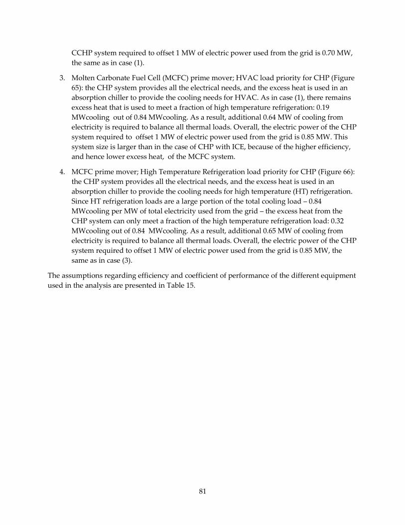
CCHP system required to offset 1 MW of electric power used from the grid is 0.70 MW, the same as in case (1).
3. Molten Carbonate Fuel Cell (MCFC) prime mover; HVAC load priority for CHP (Figure 65): the CHP system provides all the electrical needs, and the excess heat is used in an absorption chiller to provide the cooling needs for HVAC. As in case (1), there remains excess heat that is used to meet a fraction of high temperature refrigeration: 0.19 MWcooling out of 0.84 MWcooling. As a result, additional 0.64 MW of cooling from electricity is required to balance all thermal loads. Overall, the electric power of the CHP system required to offset 1 MW of electric power used from the grid is 0.85 MW. This system size is larger than in the case of CHP with ICE, because of the higher efficiency, and hence lower excess heat, of the MCFC system.
4. MCFC prime mover; High Temperature Refrigeration load priority for CHP (Figure 66): the CHP system provides all the electrical needs, and the excess heat is used in an absorption chiller to provide the cooling needs for high temperature (HT) refrigeration. Since HT refrigeration loads are a large portion of the total cooling load – 0.84 MWcooling per MW of total electricity used from the grid – the excess heat from the CHP system can only meet a fraction of the high temperature refrigeration load: 0.32 MWcooling out of 0.84 MWcooling. As a result, additional 0.65 MW of cooling from electricity is required to balance all thermal loads. Overall, the electric power of the CHP system required to offset 1 MW of electric power used from the grid is 0.85 MW, the same as in case (3).
The assumptions regarding efficiency and coefficient of performance of the different equipment used in the analysis are presented in Table 15.
81

Table 15: Parameters for the Electrical and Cooling Systems Considered in the Study
Parameter Value
Low Temperature Electric Chiller COP COPLTcool 1.60
High Temperature Electric Chiller COP COPHTcool 2.20
HVAC Electric Chiller COP COPHVAC 2.80
High Temperature Absorption Chiller COP COPabsChill, HT 0.67
HVAC Absorption Chiller COP COPabsChill, HVAC 0.75
ICE electrical efficiency ICE,elec 0.35
ICE total efficiency ICE,total 0.85
MCFC electrical efficiency MFCF,elec 0.48
MCFC total efficiency MFCF,total 0.75
Based on the analysis of the four cases presented in Table 16, the total capacity of DG/CHP units that would be required to offset electricity used from the grid depends on the prime mover and the primary use of the excess heat as presented in Table 16. Utilization of the excess heat in DG/CHP reduces the total capacity needed to provide for electrical and thermal loads. In the cases of ICE systems, the total electricity production by DG/CHP required to offset the baseline electricity of 4401 GWh/year would be 3073-3093 GWh/year. Assuming a constant power consumption throughout the year, the average capacity of DG/CHP installations would be 351-353 MW, 30 percent lower than the average baseline capacity required for food retail stores in the year 2007 (502 MW). For the cases with MCFC systems, the reduction in capacity is less pronounced than in the ICE cases, due to the higher energy efficiency of the MCFC systems. The reduction in electricity production would be 14-15 percent, requiring an average installed capacity of 427-430 MW. Assuming that an average food retail store would require a 150 kWelectric system, meeting the electricity and cooling demand would require 2338-2354 ICE units, or 2843-2867 MCFC units
82

Table 16: DG/CHP Application in Food Retail Stores in the South Coast Air Basin of California
Cases Electricity generation (GWh/year)
Average power (MW)
Number of 150 kW
installations
As Built Grid Connected case (2007) 4401 502 N/A
Case 1 ICE meeting HVAC load 3073 351 2338
Case 2 ICE meeting HT refrigeration 3093 353 2354
Case 3 MCFC meeting HVAC load 3736 427 2843
Case 4 MCFC meeting HT refrigeration 3767 430 2867
83
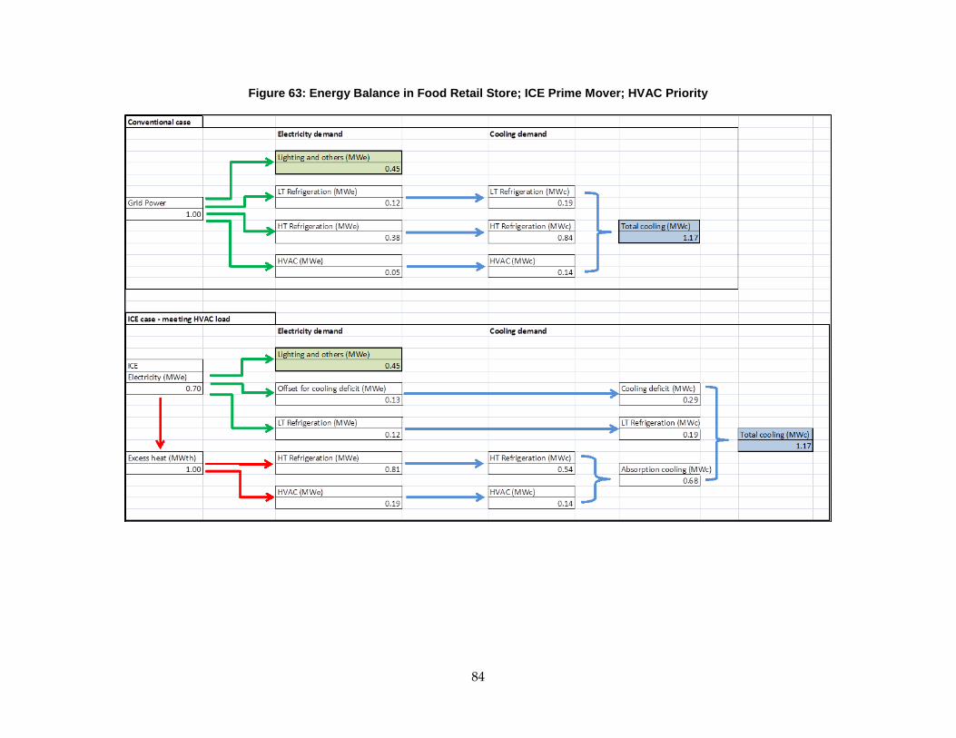
Figure 63: Energy Balance in Food Retail Store; ICE Prime Mover; HVAC Priority
84

Figure 64: Energy Balance in Food Retail Store; ICE Prime Mover; HVAC Priority
Additional cooling produced from electricity is needed to meet total high temperature refrigeration and HVAC loads
85
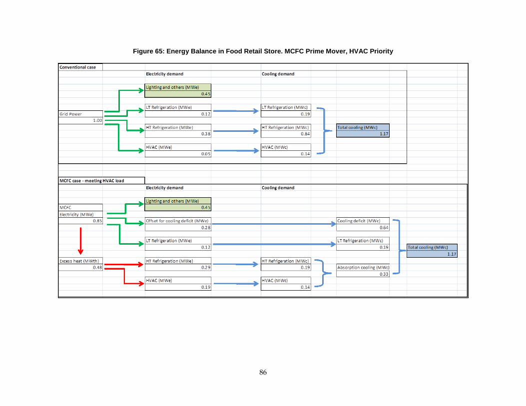
Figure 65: Energy Balance in Food Retail Store. MCFC Prime Mover, HVAC Priority
86
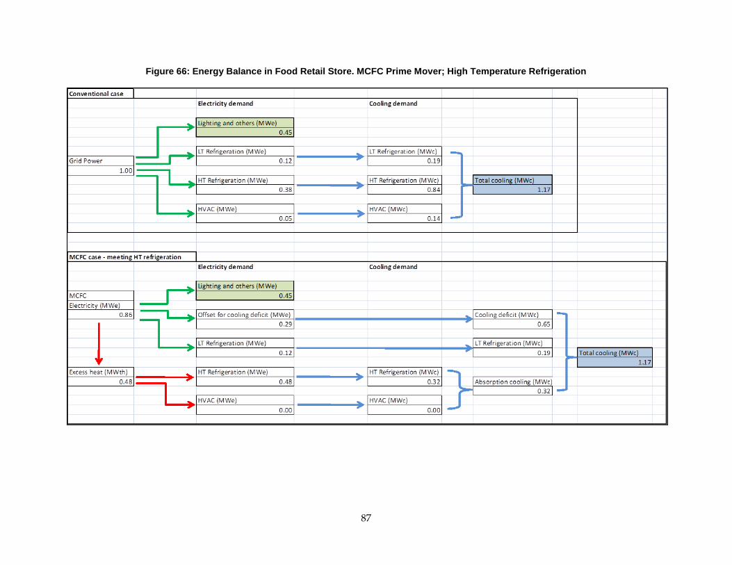
Figure 66: Energy Balance in Food Retail Store. MCFC Prime Mover; High Temperature Refrigeration
87

6.1.4 Impact of DG/CHP Deployment on Regional Air Quality This section evaluates the emission changes due to implementation of CHP systems to offset electricity use from the grid. The emission factors used in the analysis are presented in Table 17. Emissions from MCFC systems are lower than the corresponding 2007 ARB emission standards for distributed generation installations. In contrast, emissions from ICE systems do not comply with current BACT standards unless they include an after-treatment control measure. For electricity generation alone, ICE systems require a significant reduction of emissions to comply with the BACT standards. The use of CHP in ICE units allows for emission credits that equals a thermal load unit with an electric load unit. In the case of ICE CHP systems, the thermal load utilized from the ICE system is 1 MWthermal per 0.7 MWelectric (1.43 MWthermal/MWelectric). The emission credits results in an effective increase in permitted emissions of 143 percent.
Table 17: Emissions Factors for MCFC and ICE Installations
Pollutant EFMCFC
a
(lbs/MWhe) EFICE
(lbs/MWhe) EFICE-BACT
(lbs/MWhe) EFICE-CHP-BACT (lbs/MWhe)e
NOX 0.050 0.310b 0.070 0.170
CO 0.040 1.500b 0.200 0.486
VOC 0.005 0.460b 0.100 0.243
PM10 0.120c 0.013d 0.032
SO2 0.007b 0.024d 0.007
a Table 7.3, Emissions for 250kW MCFC estimated for 2010, DER Emissions Survey and Technology Characterization, E2I, 2005 b Table 6-5, Emissions for 100 kW system estimated for the year 2010, DER Emissions Survey and Technology Characterization, E2I, 2005 c Table 6-4, lower limit for PM10 emissions, DER Emissions Survey and Technology Characterization, E2I, 2005 d Based on Combined Cycle Power plant BACT e Includes CHP credits. Expressed as Minimum between EFICE and EFICE-BACT*(1+Welec/Wth)
Table 18 presents the resulting basin-wide emissions from the deployment of CHP installations. Emissions from MCFC installations are considerably lower than in the case with ICE, even though the total installed capacity in the MCFC case is 22 percent larger than the required capacity in the ICE case. Compared to the emissions from a power plant located in Huntington Beach that produce comparable power required by the conventional case, the MCFC option would result in net reduction in pollutant emissions. In contrast, the ICE option would lead to net increases in emissions. It is important to note that the emission changes due to CHP deployment are of the order of less than 0.1 percent of the total emissions in the basin from all sources.
88

Table 18: Total Emissions from Deployment of CCHP Installations in Food Retail Stores
Distributed generation with CCHP Central power planta
Pollutant MCFC meeting HT refrigeration
ICE meeting HT refrigeration
AES Huntington Beach
2005 Emissions Inventorya
Capacity (MW) 430 353 888b
Pollutant Emissions (tons/day)
NOX 0.23 0.65 0.32 746
CO 0.19 1.87 1.26 4111
VOC 0.02 0.94 0.03 1262
PM10 - 0.12 0.11 605
SO2 - 0.03 0.02 88
a Emissions extracted from the 2005 inventory provided by the South Coast Air Quality Management District b Nameplate capacity
6.1.5 Baseline Air Quality The gas-phase chemical mechanism used in the present simulations is the Caltech Atmospheric Chemical Mechanism (CACM)(Griffin et al)17 . It includes ozone (O3) chemistry and a state-of-the-art mechanism of the gas phase precursors of secondary organic aerosol (SOA). The full mechanism consists of 361 chemical reactions and 191 gas-phase species, which describe a comprehensive treatment of VOCs oxidation. The model includes 37 size-resolved aerosol-phase species, in 8 different size bins ranging from 0.04 to 10 microns.
The grid used by the UCI-CIT model encompasses Orange County and part of Los Angeles, Ventura, San Bernardino, and Riverside counties (Figure 67). The grid consists of cells with an area of 25 km2. Additionally the vertical resolution is described through five vertical layers with the following dimensions from ground level up: (1) 0 m–39 m, (2) 39 m–154 m, (3) 154 m–308 m, (4) 308 m–671 m, and (5) 671 m–1100 m.
17 Griffin, R.J., Dabdub, D., Seinfeld, J.H., 2002a. Secondary organic aerosol. 1. Atmospheric chemical mechanism for production of molecular constituents. Journal of Geophysical Research 107(D17), 4332
89

Figure 67: UCI-CIT Airshed Modeling Domain of the South Coast Air Basin of California
Meteorological conditions were obtained during the Southern California Air Quality Study (SCAQS), which was a comprehensive campaign of atmospheric measurements that took place in the SoCAB during August 27–29, 1987. In addition, the August 27–28, 1987 episode is statistically within the top 10 percent of severe ozone-forming meteorological conditions. Hence, meteorological conditions for August 27-29 are used here as the basis to evaluate air quality impacts of DG.
The SCAQS episode in August 27–29, 1987 was characterized by a weak onshore pressure gradient and warming temperatures aloft. The wind flow was characterized by a sea breeze during the day and a weak land-mountain breeze at night. The presence of a well-defined diurnal inversion layer at the top of neutral and unstable layers near the surface, along with a slightly stable nocturnal boundary layer, facilitated the accumulation of pollutants over the SoCAB, which lead to a high ozone concentration occurrence.
The emissions were obtained from the South Coast Air Quality Management District (AQMD). The emissions correspond to a summer episode in 2005 that was included in the 2007 Air Quality Management Plan developed by the AQMD to demonstrate attainment of the 8-hour ozone standard. Total basin-wide emissions for this episode are presented in Table 18.
The resulting peak 8-hour ozone and 24-hour PM2.5 average concentrations are shown in Figure 68. Ozone concentration peaks downwind from Los Angeles, on the northeastern corner of the domain. Maximum PM2.5 concentrations occur near Riverside, where the ammonia emitted from agricultural and dairy activities react with nitric acid formed from NOX emitted upwind. The result is the formation of secondary ammonium nitrate particles. A secondary PM2.5 peak occurs near the port of Long Beach, where there are high emissions of particles and sulfur oxides (SOX).
90
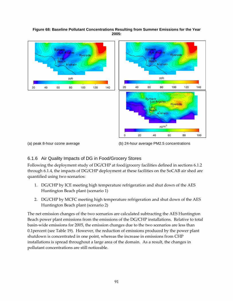
Figure 68: Baseline Pollutant Concentrations Resulting from Summer Emissions for the Year 2005:
(a) peak 8-hour ozone average (b) 24-hour average PM2.5 concentrations
6.1.6 Air Quality Impacts of DG in Food/Grocery Stores Following the deployment study of DG/CHP at food/grocery facilities defined in sections 6.1.2 through 6.1.4, the impacts of DG/CHP deployment at these facilities on the SoCAB air shed are quantified using two scenarios:
1. DG/CHP by ICE meeting high temperature refrigeration and shut down of the AES Huntington Beach plant (scenario 1)
2. DG/CHP by MCFC meeting high temperature refrigeration and shut down of the AES Huntington Beach plant (scenario 2)
The net emission changes of the two scenarios are calculated subtracting the AES Huntington Beach power plant emissions from the emissions of the DG/CHP installations. Relative to total basin-wide emissions for 2005, the emission changes due to the two scenarios are less than 0.1percent (see Table 19). However, the reduction of emissions produced by the power plant shutdown is concentrated in one point, whereas the increase in emissions from CHP installations is spread throughout a large area of the domain. As a result, the changes in pollutant concentrations are still noticeable.
91

Table 19: Net Changes in Emissions Due to Two CHP Scenarios, in Percentage (%) with Respect to Total Basin-Wide Emissions in the South Coast Basin of California in the Year 2005
Net emissions changes in % with respect to total 2005 emissions
Pollutant Scenario 1:
ICE - AES Huntington Beach Scenario 2:
MCFC - AES Huntington Beach
NOX 0.04 -0.01
CO 0.01 -0.03
VOC 0.07 0.00
PM10 0.00 -0.02
SO2 0.01 -0.02
The changes in 8-hour average O3 and 24-hour average PM2.5 concentrations caused by scenario 1 and scenario 2 are presented in Figure 69 and Figure 70, respectively. The removal of the central power plant leads to a reduction in 8-hour average O3 of 3 ppb (Figure 69a and Figure 70a), and a reduction in 24-hour average PM2.5 of 1 g/m3 (Figure 69b and Figure 70b). The 8 hour average O3 reductions occur around and immediately off shore of the power plant location and admittedly are not directly beneficial to the population. However, the effects of the substitution of one central power plant for multiple DG/CHP system on 24 hour PM2.5 levels are more apparent with both positive and negative effects. There are minor differences in the air quality impacts between the ICE and the MCFC. In both cases, there is only a slight increase in ozone concentration of less than 1 ppb downwind from Riverside, and mixed increases and decrease in PM2.5 concentrations of the order 1 g/m3. Decreases in PM2.5 are attributed to reduction in secondary formation due to the shutdown of the power plant, whereas increases in PM2.5 are attributed to increases in PM emissions and secondary formation due to emissions from DG/CHP installations.
92

Figure 69: ICE DG/CHP Application in Food/Grocery: Changes in Pollutant Concentrations
(a) effects on peak 8-hour ozone concentrations (b) effects on 24-hour average PM2.5
Figure 70: MCFC DG/CHP Application in Food/Grocery: Changes in Pollutant Concentrations:
(a) effects on peak 8-hour ozone concentrations (b) effects on 24-hour average PM2.5
6.1.7 Conclusions For the application of DG/CHP at food/grocery stores on a basin wide level, the impact of extensive deployment of DG/CHP in that sector can replace one or more of the large central power plants in the SoCAB. Analysis of energy balances suggests that DG/CHP could meet a large fraction of the high temperature refrigeration needs in addition to all the electric loads. As a result, DG/CHP systems could reduce the installed grid’s generation capacity fraction needed to provide the same electric and thermal loads to retail food/grocery stores. DG/CHP systems with internal combustion engines could reduce the grid supplied power by 30 percent, whereas as DG/CHP systems with molten carbonate fuel cells could reduce the need by 15 percent. The difference in the percentages for these two technologies for this sector is associated with the relative amount of electricity and heating/cooling required. For this sector, internal combustion engines better match these relative needs.
Owing to the relatively low number of applications as compared to the total basin energy consumption (3.6 percent), the effect on the overall air quality as measured by ozone and PM2.5 is zero to slight improvement relative to the pre-deployment situation. The impacts in
93

emissions are in general small, if compared with total emissions from all sources in the basin. The emission changes due to the deployment of DG/CHP and the removal of a central power plant correspond to less than 0.1 percent of the total basin-wide emissions. However, the reduction of emissions produced by the power plant shutdown is concentrated in one point, whereas the increase in emissions from DG/CHP installations is spread throughout a large area of the domain. As a result, the changes in pollutant concentrations are still noticeable.
The removal of the power plant produces a reduction in 8-hour average O3 and in 24-hour average PM2.5 of 3 ppb and 1 µg/m3, respectively, in the proximity of the power plant. In contrast, increases in 8-hour average O3 and in 24-hour average PM2.5 attributed to DG/CHP occur in areas around Riverside, and are of the order of 1 ppb and 1 µg/m3.
6.2 Near Field Air Quality Impacts Modeling The deployment of DG/CHP systems throughout the California electric grid has great value to improving overall energy efficiency, reducing greenhouse gas emissions, and, as shown in section 6.1, can provide overall improvement to the air quality in an air shed region. However, DG/CHP systems, as a result of their small size and specific application of distributed generation at or near the point of use, can and will be close to the people, whether facility workers or the public in general. Further, unlike central power plants and other grid support power generation system (e.g. peaker units) that tend to have tall to very tall exhaust stacks (order(s) of magnitude greater than the height of a human) to help in the plume dispersion, DG/CHP systems typically have of exhausts streams that are much closer to the height of a human. Hence, without a tall stack to help in plume dispersion and emission concentration reduction, there is a concern relative to DG/CHP system exhaust emissions contributing to air pollution in the immediate vicinity of the system exceeding the AAQS. To assess the potential effect, computational fluid dynamic modeling (CFD) of the DG/CHP (in this analysis, a Capstone C60 microturbine) system and its plume dispersion was performed to assess the mixing, dilution, and the nominal concentration of the pollutants at an elevation of 5 ft (typical human height). The lower stack height of DG is significant as typical plume dispersion modeling for power plants have stack heights of 100+ ft with predicted concentrations of the plume at the point of contact with the ground (e.g. 0 ft). Considering the reduction in concentrations from the very tall stack heights, the difference between ground level and 5 ft is not crucial. However, when the stack height is on the same order as the receptor height, evaluation of the concentrations at receptor height is logical. It is noted that the analysis carried out is specific to the Capstone C-60 microturbine and the emission levels from the device have been assumed to be the manufacturer’s stated levels (e.g., NOx at 10 ppm). Hence any conclusions drawn from this analysis must be caveated by these assumptions. It is also noted that examples of DG/CHP systems falling out of compliance during operation (Kay)1, (Mueller et al)18 have been identified with the implication that policy towards ensuring that compliance is maintained is needed.
18 Mueller, Marla, Mark Wilson, Nicole Davis, Ed Vine, Jim Lents, Jan Sharpless. 2008. Impacts of Distributed Generation on Air Quality: A Roadmap. California Energy Commission, PIER Energy‐Related Environmental Research Program. CEC‐500‐2008‐022
94

6.2.1 Modeling Conditions In this work, the NOx dispersion from a typical microturbine generator (MTG) is studied. There are numerous parameters that can affect the plume dispersion near a MTG: local wind speed and direction, exhaust temperature, exhaust NOx concentration, exhaust velocity, direction of exhaust velocity and proximity to a wall. In this study, the effects of exhaust velocity, (both magnitude and direction/deflection of exhaust), exhaust height relative to the ground, wind speed, and proximity to two different shapes of wall are examined.
6.2.2 Domain and Grid Generation The dimensions of the domain that includes the micro turbo generator (MTG) are defined in a way to make sure the boundaries don’t have considerable effects on flow field. Therefore, based on preliminary studies, these dimensions are picked for this study, as shown in Table 20, and Figure 71 are relatively large as compared to the microturbine. Ultimately, the results indicate that the Y and Z directions as defined are larger than necessary by a factor of two and as such the defined boundaries in these directions are sufficiently “distant” from the plume source that they do not affect the calculated plume dispersion
Accurate computations of turbulent flows require careful mesh generation. While high accuracy is desired, turbulent fluctuations play a significant role in the transport of all parameters. Consequently, it is critical to ascertain that the turbulent quantities are suitably resolved. Due to the strong interaction of the mean flow and turbulence, numerical results for turbulent flows, especially mass transport results, are more sensitive to grid quality dependency than those for laminar flows.
95
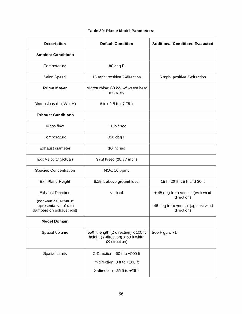
Table 20: Plume Model Parameters:
Description Default Condition Additional Conditions Evaluated
Ambient Conditions
Temperature 80 deg F
Wind Speed 15 mph; positive Z-direction 5 mph, positive Z-direction
Prime Mover Microturbine; 60 kW w/ waste heat recovery
Dimensions (L x W x H) 6 ft x 2.5 ft x 7.75 ft
Exhaust Conditions
Mass flow ~ 1 lb / sec
Temperature 350 deg F
Exhaust diameter 10 inches
Exit Velocity (actual) 37.8 ft/sec (25.77 mph)
Species Concentration NOx: 10 ppmv
Exit Plane Height 8.25 ft above ground level 15 ft, 20 ft, 25 ft and 30 ft
Exhaust Direction
(non-vertical exhaust representative of rain
dampers on exhaust exit)
vertical + 45 deg from vertical (with wind direction)
-45 deg from vertical (against wind direction)
Model Domain
Spatial Volume 550 ft length (Z direction) x 100 ft height (Y-direction) x 50 ft width
(X-direction)
See Figure 71
Spatial Limits Z-Direction: -50ft to +500 ft
Y-direction; 0 ft to +100 ft
X-direction; -25 ft to +25 ft
96

Description Default Condition Additional Conditions Evaluated
Location of exhaust Z=0, X=0, Y = 8.25 Y=15ft , 20ft, 25ft, and 30ft
Flow Field Unobstructed (semi-infinite) Full Wall: Upstream “building”, full extent in X-direction, 25 ft tall in Y-direction, location from Z= -50 ft to -15 ft
Half Wall: Upstream building, half of x-domain (X=0 to X=25 ft), 25 ft tall, location from Z=-50 ft to -15 ft
Boundary Conditions -Ground: Wall (no transport)
-Top: Pressure outlet (0 psi gauge)
Lateral Sides (XZ planes): Velocity Inlet (tangential velocity = wind
speed)
Wind Entrance plane (XY plane): Velocity Inlet
Wind Exit plane (XY plane): Pressure outlet (0 psi gauge)
97

Figure 71: Domain for Analysis (not to scale)
The grid for the current investigation was created using unstructured tetrahedral mesh elements. Due to the symmetric domain for most of the cases, the mesh is generated in half of the domain in those cases and a “symmetric” or mirror image boundary condition applied. However, for the cases without a symmetric domain condition, the mesh is generated for the entire domain. To capture more information along the path of the exhaust of MTG in the region of the non-symmetrical domain (i.e. the asymmetric wall) an adaptive grid was utilized to refine the mesh in this region. All computations are carried out on an 8 node Beowulf cluster each with 4 GB RAM. The CPUs are AMD Opteron 2.6GHz CPUs with 1MB cache. The operating system is Redhat 4 64 bit OS Advance Server and the nodes are connected via a GigE Nortel switch.
Table 20 identifies the breadth of the parameter variations identified for the analysis. Table 21 identifies the specific cases and conditions for the analyses as well as some information on the gridding and the iterations of the analyses necessary for proper convergence of the models.
98
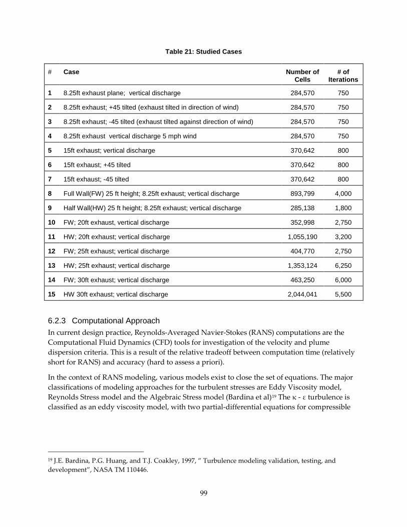
Table 21: Studied Cases
# Case Number of Cells
# of Iterations
1 8.25ft exhaust plane; vertical discharge 284,570 750
2 8.25ft exhaust; +45 tilted (exhaust tilted in direction of wind) 284,570 750
3 8.25ft exhaust; -45 tilted (exhaust tilted against direction of wind) 284,570 750
4 8.25ft exhaust vertical discharge 5 mph wind 284,570 750
5 15ft exhaust; vertical discharge 370,642 800
6 15ft exhaust; +45 tilted 370,642 800
7 15ft exhaust; -45 tilted 370,642 800
8 Full Wall(FW) 25 ft height; 8.25ft exhaust; vertical discharge 893,799 4,000
9 Half Wall(HW) 25 ft height; 8.25ft exhaust; vertical discharge 285,138 1,800
10 FW; 20ft exhaust, vertical discharge 352,998 2,750
11 HW; 20ft exhaust; vertical discharge 1,055,190 3,200
12 FW; 25ft exhaust; vertical discharge 404,770 2,750
13 HW; 25ft exhaust; vertical discharge 1,353,124 6,250
14 FW; 30ft exhaust; vertical discharge 463,250 6,000
15 HW 30ft exhaust; vertical discharge 2,044,041 5,500
6.2.3 Computational Approach In current design practice, Reynolds-Averaged Navier-Stokes (RANS) computations are the Computational Fluid Dynamics (CFD) tools for investigation of the velocity and plume dispersion criteria. This is a result of the relative tradeoff between computation time (relatively short for RANS) and accuracy (hard to assess a priori).
In the context of RANS modeling, various models exist to close the set of equations. The major classifications of modeling approaches for the turbulent stresses are Eddy Viscosity model, Reynolds Stress model and the Algebraic Stress model (Bardina et al)19 The κ - ε turbulence is classified as an eddy viscosity model, with two partial-differential equations for compressible
19 J.E. Bardina, P.G. Huang, and T.J. Coakley, 1997, ” Turbulence modeling validation, testing, and development”, NASA TM 110446.
99

and incompressible fluids (ibid)20. The Realizable κ - ε model, as used in this effort, is reportedly the most reliable κ - ε turbulence model for the jet in cross flow problem (Xaio)21.
Governing Equations and Flow Analysis.
Since some features of the flow field can be interpreted by means of looking at the role of different parameters in the governing equation, those associated with the κ - ε turbulence model are discussed. For an incompressible steady flow with constant viscosity, the Reynolds averaged governing equations for mass, momentum, species concentration, turbulent kinetic (FLUENT) 𝜕𝜕𝑥𝑖
(𝜌𝑈𝑖Ψ) = 𝜕𝜕𝑥𝑖
�𝐷Ψ𝜕Ψ𝜕𝑥𝑖�+ 𝑆Ψ (1)
The equations are specified in detail in Table 22. It should be noted that Ψ is an arbitrary variable which can be replaced with an appropriate variable according to Table 22 and DΨ is the diffusion term.
Table 22: Detailed Governing Equations
𝜇𝑡,, which is the turbulent viscosity, is defined as:
𝜇𝑡 = 𝐶𝜇𝜌𝑘2/𝜀 (2)
Where 𝐶𝜇=0.09, 𝑐1=1.44, 𝑐2=1.92, 𝜎𝑘=1.0 and 𝜎𝜀=1.3. S represents the species concentration and 〖𝑆𝑐𝑡 is the turbulent Schmidt number.
20 Y. Xiao and H.W. Tang, 2006, “Numerical simulation of a horizontal momentum jet in cross-flow”, J. Hydrodynamics, Vol 18, pp. 118-125.
21 FLUENT 6.3 Documentation
Ψ 𝑫𝚿 𝑺𝚿
1 0 0
𝑼𝒋,j=1,2,3 𝜇𝑡 −𝜕𝑃/𝜕𝑥𝑗+ 𝜕{𝜇𝑡(𝜕𝑈𝑖/𝜕𝑥𝑗)}/ 𝜕𝑥𝑖
S 𝜇𝑡/𝑆𝑐𝑡 0
k 𝜇𝑡/𝜎𝑘 𝐺 − 𝜌𝜀
𝜺 𝜇𝑡/𝜎𝜀 (𝜀/𝑘)(𝑐1𝐺 − 𝑐2𝜌𝜀)
100
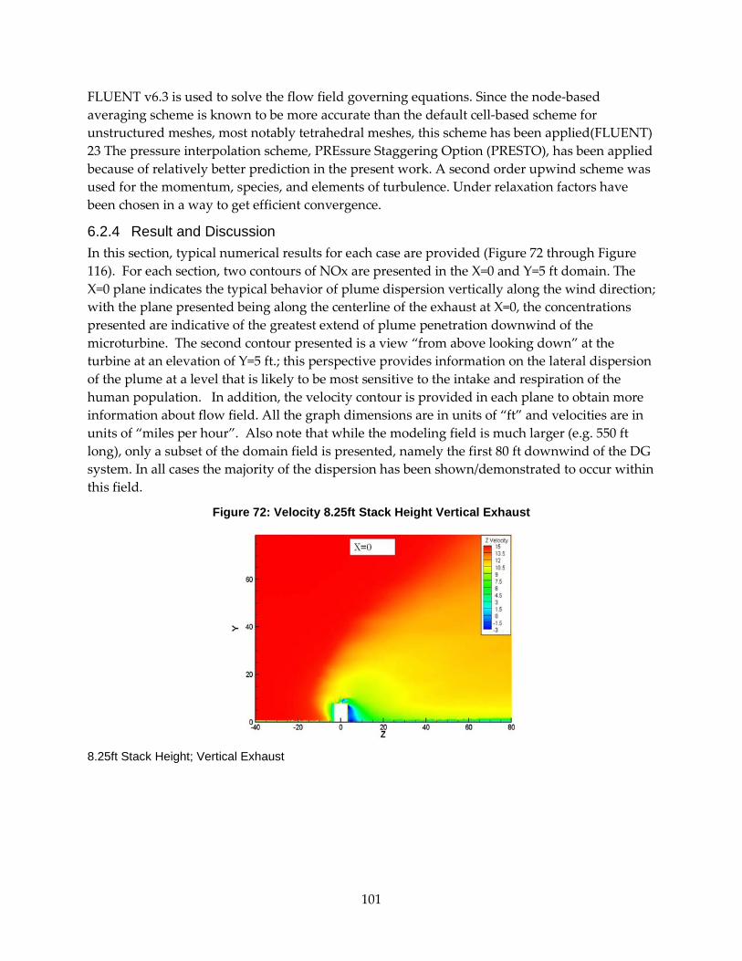
FLUENT v6.3 is used to solve the flow field governing equations. Since the node-based averaging scheme is known to be more accurate than the default cell-based scheme for unstructured meshes, most notably tetrahedral meshes, this scheme has been applied(FLUENT) 23 The pressure interpolation scheme, PREssure Staggering Option (PRESTO), has been applied because of relatively better prediction in the present work. A second order upwind scheme was used for the momentum, species, and elements of turbulence. Under relaxation factors have been chosen in a way to get efficient convergence.
6.2.4 Result and Discussion In this section, typical numerical results for each case are provided (Figure 72 through Figure 116). For each section, two contours of NOx are presented in the X=0 and Y=5 ft domain. The X=0 plane indicates the typical behavior of plume dispersion vertically along the wind direction; with the plane presented being along the centerline of the exhaust at X=0, the concentrations presented are indicative of the greatest extend of plume penetration downwind of the microturbine. The second contour presented is a view “from above looking down” at the turbine at an elevation of Y=5 ft.; this perspective provides information on the lateral dispersion of the plume at a level that is likely to be most sensitive to the intake and respiration of the human population. In addition, the velocity contour is provided in each plane to obtain more information about flow field. All the graph dimensions are in units of “ft” and velocities are in units of “miles per hour”. Also note that while the modeling field is much larger (e.g. 550 ft long), only a subset of the domain field is presented, namely the first 80 ft downwind of the DG system. In all cases the majority of the dispersion has been shown/demonstrated to occur within this field.
Figure 72: Velocity 8.25ft Stack Height Vertical Exhaust
8.25ft Stack Height; Vertical Exhaust
101

Figure 73: NOx Concentration for 8.25ft Stack Height Vertical Exhaust
Figure 74: NOx Concentration; Y=5ft for 8.25ft Stack Height Vertical Exhaust
Figure 75: Velocity for 8.25ft Stack Height +45 Tilted
102
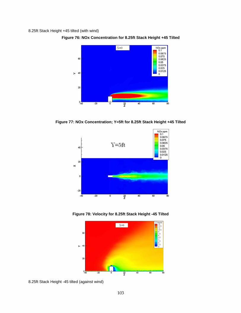
8.25ft Stack Height +45 tilted (with wind)
Figure 76: NOx Concentration for 8.25ft Stack Height +45 Tilted
Figure 77: NOx Concentration; Y=5ft for 8.25ft Stack Height +45 Tilted
Figure 78: Velocity for 8.25ft Stack Height -45 Tilted
8.25ft Stack Height -45 tilted (against wind)
103
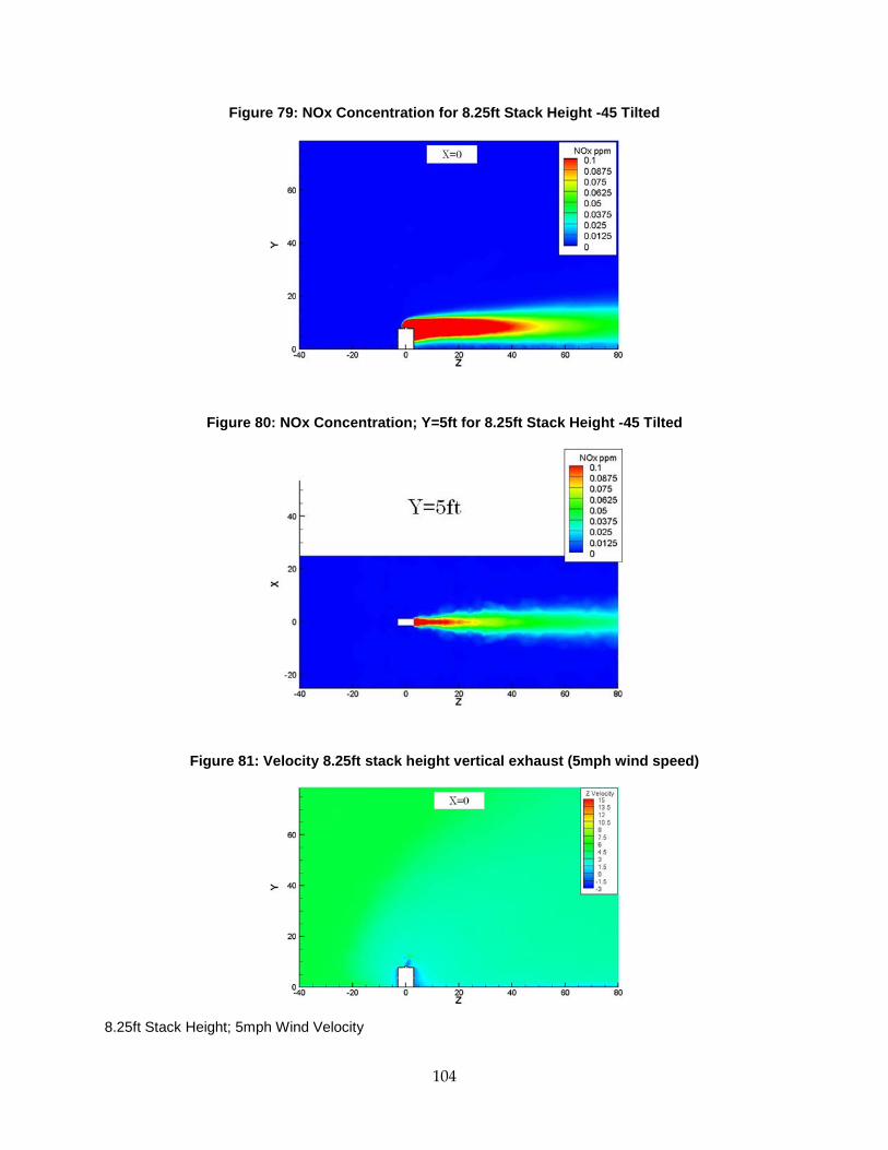
Figure 79: NOx Concentration for 8.25ft Stack Height -45 Tilted
Figure 80: NOx Concentration; Y=5ft for 8.25ft Stack Height -45 Tilted
Figure 81: Velocity 8.25ft stack height vertical exhaust (5mph wind speed)
8.25ft Stack Height; 5mph Wind Velocity
104
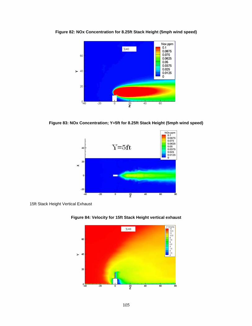
Figure 82: NOx Concentration for 8.25ft Stack Height (5mph wind speed)
Figure 83: NOx Concentration; Y=5ft for 8.25ft Stack Height (5mph wind speed)
15ft Stack Height Vertical Exhaust
Figure 84: Velocity for 15ft Stack Height vertical exhaust
105

Figure 85: NOx Concentration for 15ft Stack Height vertical exhaust
Figure 86: NOx Concentration; Y=5ft for 15ft Stack Height
15ft Stack Height +45 tilt (with wind)
Figure 87: Vertical velocity for 15ft Stack Height +45 tilted
106
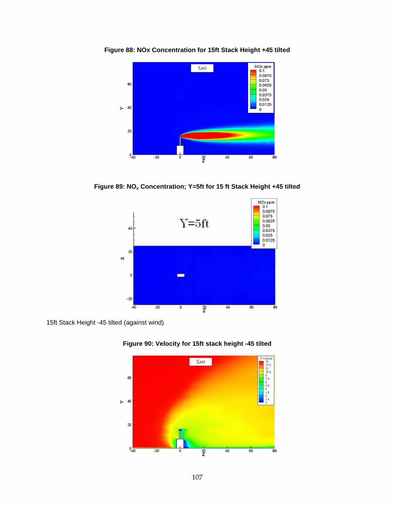
Figure 88: NOx Concentration for 15ft Stack Height +45 tilted
Figure 89: NOx Concentration; Y=5ft for 15 ft Stack Height +45 tilted
15ft Stack Height -45 tilted (against wind)
Figure 90: Velocity for 15ft stack height -45 tilted
107

Figure 91: Velocity for 15ft stack height -45 tilted
Figure 92: NOx Concentration for 15ft Stack Height -45 tilted
25ft Height full wall (FW), 8.25ft Stack Height
Figure 93: Velocity for FW, 8.25ft stack height
108

Figure 94: NOx Concentration for FW, 8.25ft stack height
Figure 95: NOx Concentration; Y=5ft for FW, 8.25ft stack height
25ft Height Half Wall (HW), 8.25ft Stack Height
Figure 96: Velocity for HW, 8.25ft stack height
109
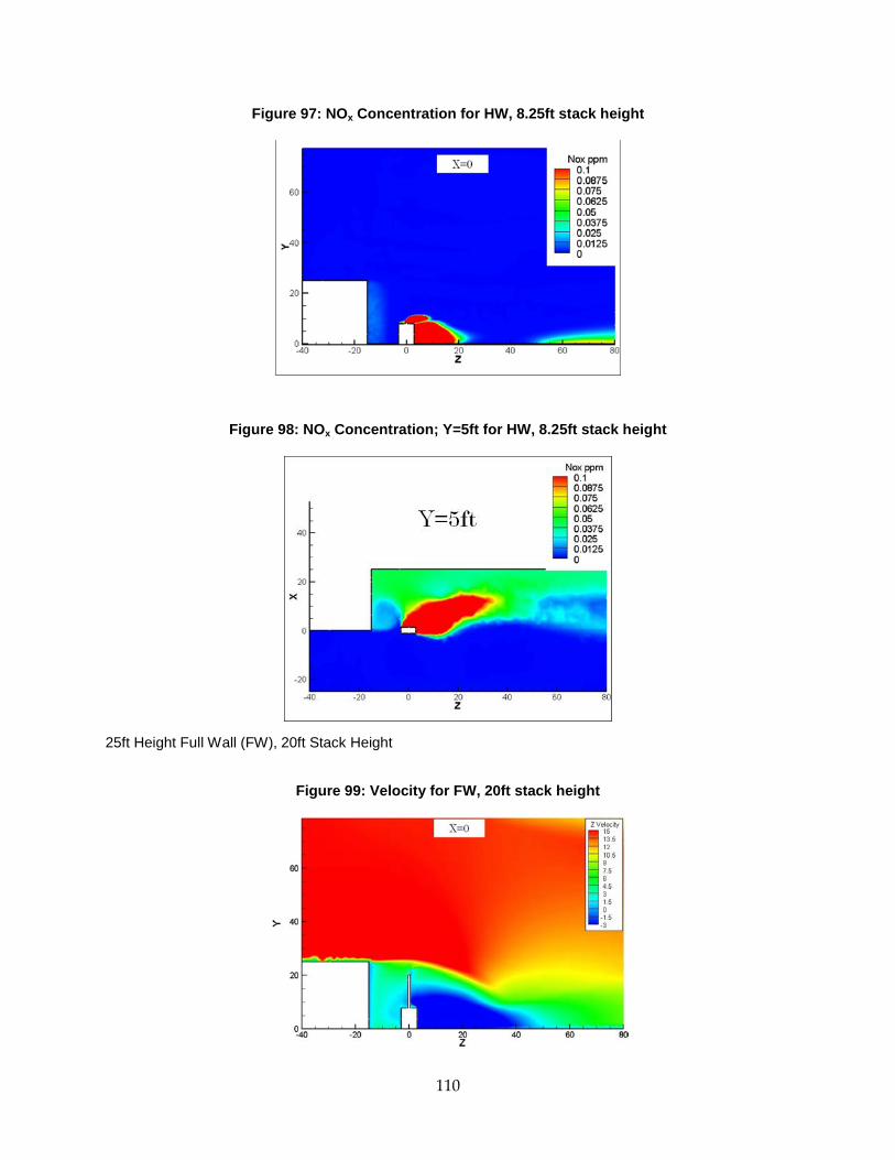
Figure 97: NOx Concentration for HW, 8.25ft stack height
Figure 98: NOx Concentration; Y=5ft for HW, 8.25ft stack height
25ft Height Full Wall (FW), 20ft Stack Height
Figure 99: Velocity for FW, 20ft stack height
110
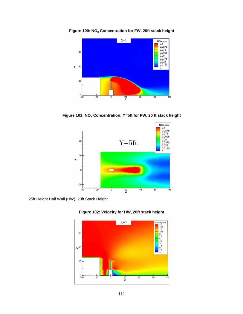
Figure 100: NOx Concentration for FW, 20ft stack height
Figure 101: NOx Concentration; Y=5ft for FW, 20 ft stack height
25ft Height Half Wall (HW), 20ft Stack Height
Figure 102: Velocity for HW, 20ft stack height
111

Figure 103: NOx Concentration for HW, 20ft stack height
Figure 104: NOx Concentration; Y=5ft for HW, 20ft stack height
25ft Height Full Wall (FW), 25ft Height
Figure 105: Velocity for FW, 25ft stack height
112
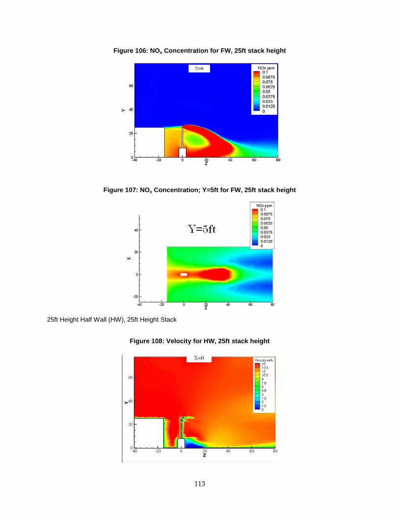
Figure 106: NOx Concentration for FW, 25ft stack height
Figure 107: NOx Concentration; Y=5ft for FW, 25ft stack height
25ft Height Half Wall (HW), 25ft Height Stack
Figure 108: Velocity for HW, 25ft stack height
113
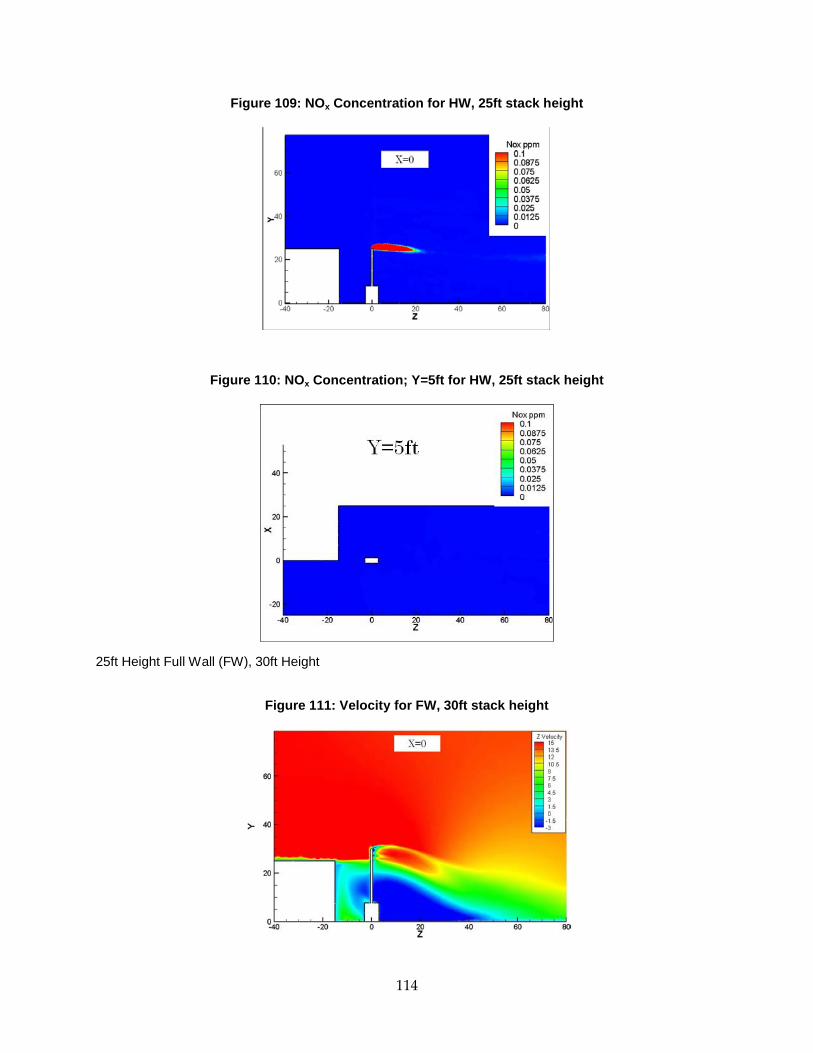
Figure 109: NOx Concentration for HW, 25ft stack height
Figure 110: NOx Concentration; Y=5ft for HW, 25ft stack height
25ft Height Full Wall (FW), 30ft Height
Figure 111: Velocity for FW, 30ft stack height
114

Figure 112: NOx Concentration for FW, 30ft stack height
Figure 113: NOx Concentration; Y=5ft for FW, 30ft stack height
25ft Height Half Wall (HW), 30ft Height
Figure 114: Velocity for HW, 30ft stack height
115

Figure 115: NOx Concentration for HW, 30ft stack height
Figure 116: NOx Concentration; Y=5ft for HW, 30ft stack height
6.2.5 Conclusions The effects of DG/CHP on both the near field adjacent to the system and the South Coast Air Basin (SoCAB) were analyzed through computer modeling. The results suggest very rapid dispersion of the plume. In the presented results, it is vital to note that the “red” section in the above figures showing NOx concentrations represents a minimum concentration of 0.1 ppm NOx, two orders of magnitude lower than the exhaust gas concentration. The presence of upstream obstructions such as a building or a wall does result in a more disrupted field and greater near field impact. However, mixing and dispersion are still quite rapid and the resulting concentration levels are not greatly increased as compared to the cases where there were no obstructions upstream. Overall the microturbine exhaust has minimal effect on the near field concentration levels at human population impact elevations. However, when compared to the current California Ambient Air Quality Standard of 0.18 ppm for 1 hour or the
116

new Environmental Protection Agency (EPA) standard of 0.1 ppm for 1 hour, the contribution from the microturbine are on the order of these limits. In most cases the addition of DG/CHP will not result in exceeding air quality standards, but when combined with already high ambient air pollution levels, the impact of the microturbine may result in some local areas exceeding the limits.
Another pertinent observation is that, as previously stated, the dispersion as modeled in these simplistic cases is very rapid. Essentially all of the dispersion and region of influence occurs within 100 ft of the DG stack. As noted, the effect of specific buildings and multiple buildings as well as other meteorological influences such as vertical mixing from ground radiation effects have not been included. The myriad of possible scenarios is unbounded. Scale modeling performed suggests a radius to stack height ratio of approximately 50 – 100 as the limit of direct influence of DG sources (Mueller).20 This would suggest a distance of 400 – 800 ft (120 – 240 meters). Yet, the modeling results suggest that the real world would expect increased flow perturbation and mixing and hence would suggest even faster dispersion of the plume limiting the influence to within a 100 ft distance. In an effort to bridge the two lines of thinking, for the sake of this analysis of the near-field population exposure, a distance of 100 meters (328 ft) from the DG stack will be considered in this analysis as the near field.
6.3 Near Field Population Analysis With an understanding of the extent of potential plume influence, the effect of the widespread deployment of DG/CHP on resident permanent population was evaluated. This evaluation was limited to Southern California, a region for which extensive geographical information system (GIS) data was readily available. The region evaluated represents an area of 96.17 billion square meters and has a population of 17.9 million.
The results of the effort are based upon the GIS information on population density within sectors (zip-codes), the location and shape of facilities in the six sectors of interest, and the intersection /overlap of the permanent residential zones as defined by GIS with the 100 meter extension of the boundaries of the facilities defined on the GIS map. Note that the data identifies permanent population. There is no way within the GIS to understand the transient population that might be influence by the presence of a DG system. For example, the GIS analysis permitted identification of the number of permanent population that was within the 100 meter boundary of a hospital’s region of influence but does not address the number of patients, staff, or people visiting a hospital during the day, all considered to be transient rather than permanent residents.
Another caveat relative to the analysis is that the population identified was based upon the geographical overlay of the facility’s region of influence with the permanent residential map. There was no analysis of meteorological effects, primarily wind, nor abnormalities of the weather condition to generate a subset of the field of influence consistent with prevailing weather conditions. It is understood that consideration of the prevailing winds would greatly reduce the affected population.
117
Finally, of the six sectors of interest to the program (hotels, hospitals, large commercial offices, jails/prisons, colleges/universities, and food/grocery stores), the impacts of food/grocery stores were not included in the analysis. The GIS data base available for the analysis did not discriminate grocery stores from other “retail” facilities (strip malls, large retail, etc.). Since grocery stores comprise only a fraction of the retail sector, inclusion of all retail in the analysis would unrealistically skew the results to larger affected population. As such, the impact of grocery stores, expected to actually have more influence per facility on resident population than most of the other sectors given the service to residents and proximity to residential areas, could not be directly assessed.
6.3.1 GIS Field The analysis of DG/CHP deployment affected population was limited to the Southern California region as defined in Figure 117. The analysis required three data sets:
• Land use definition
• Geographical shape files.
• US Census demographic census data
The land use definition was used to discriminate between the “business” land use for a variety of sectors, including those of interest to this program and residential areas. The spatial mapping of land use in the southern California region was initially developed by Aerial Information Systems, Inc. (AIS) for the Southern California Association of Governments (SCAG) in 1990. This data has been periodically updated, with the most recent update in 2005 (used in this analysis). The data is collected using aerial photography, computer based photo interpretation techniques, and digital natural color imagery. The “hard to identify photo signatures” were flagged for on-site visits performed by AIS field survey teams to ensure the accuracy of the interpretations. (Web link: http://www.aisgis.com/projects/SCAG.html)
The Topologically Integrated Geographic Encoding and Referencing (TIGER) database is a digital database of geographic features covering the entire United States. They can be downloaded publically as shape files which run in software based geographical information systems (GIS). TIGER files are developed and updated periodically by the US Census bureau; the data used in this report is from 2005. The shape files do not include demographic data, but it can be linked to the Census Bureau’s demographic data (US Census Web site)22.
The US Census data base is used in conjunction with the TIGER shape files to create a spatially resolute demographical file which can be inputted into GIS.
22 Web link: http://www.census.gov/geo/www/tiger/overview.html
118

Figure 117: Map of Analysis Area
119

6.3.2 Analysis For the analysis, DG/CHP systems were assumed to be installed at all facilities representative of the sectors of interest in this study;
• Commercial office buildings of all heights (Note that the program identified large commercial office which is facilities greater than 100,000 sq-ft. However, GIS does not provide this discrimination but rather one based upon building height with the choices of 1to 10 stories, 11 to 40 stories, and more than 40 stories.)
• Universities and colleges
• Hospitals and major health care facilities
• Hotels and motels
• Correctional facilities (jails/prisons)
As previously mentioned, food/grocery stores were not included in the analysis. The SCAG land use database aggregated food/grocery stores under the generic heading of “retail stores” and they could not be separately resolved.
Locations of all five facility types were mapped on ArcGIS. These sites were mapped using the 2005 SCAGLU database and expressed as a 2D polygons with discrete areas. Of the mapped sites, all of them were given a 100 meter (real world) buffer around their perimeters. Using this buffer, the mapped sites were increased to include the 100 meter buffer. Figure 118 is an example of a set of hotel buildings in Anaheim. The dark blue are the actual land areas of the buildings while the lighter blue regions are the 100 meter buffer that was imposed onto the actual building.
Figure 118: Example – Hotel Buildings for DG Siting
120
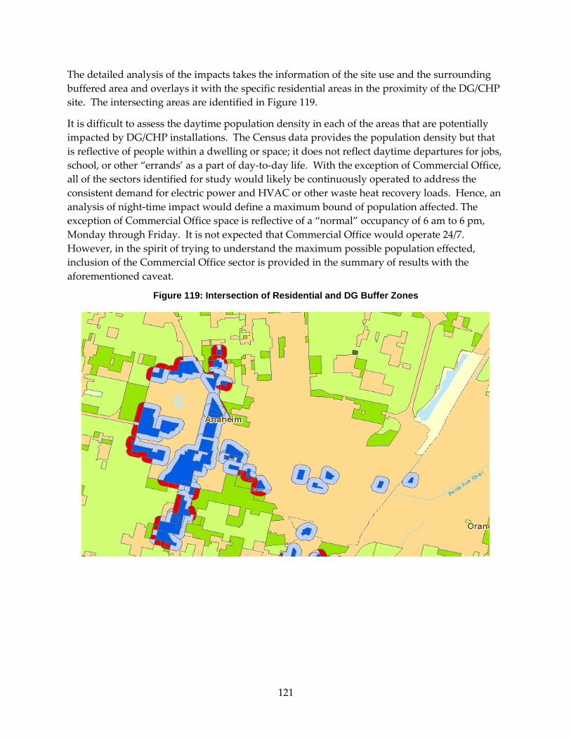
The detailed analysis of the impacts takes the information of the site use and the surrounding buffered area and overlays it with the specific residential areas in the proximity of the DG/CHP site. The intersecting areas are identified in Figure 119.
It is difficult to assess the daytime population density in each of the areas that are potentially impacted by DG/CHP installations. The Census data provides the population density but that is reflective of people within a dwelling or space; it does not reflect daytime departures for jobs, school, or other “errands’ as a part of day-to-day life. With the exception of Commercial Office, all of the sectors identified for study would likely be continuously operated to address the consistent demand for electric power and HVAC or other waste heat recovery loads. Hence, an analysis of night-time impact would define a maximum bound of population affected. The exception of Commercial Office space is reflective of a “normal” occupancy of 6 am to 6 pm, Monday through Friday. It is not expected that Commercial Office would operate 24/7. However, in the spirit of trying to understand the maximum possible population effected, inclusion of the Commercial Office sector is provided in the summary of results with the aforementioned caveat.
Figure 119: Intersection of Residential and DG Buffer Zones
121

The detailed night time approach makes a highly resolute estimate of the total number of people that could be affected at night by the installation of DG/CHP at the potential sites. The assumption made for the night time analysis is that all of the night time population is distributed in residential buildings. Although this is not strictly true, it can be assumed that the majority of the population is asleep in a residential building at these times.
The first step in this analysis was to redistribute the average population density of a zip code to population densities of different residential areas within that zip code. Four discrete residential areas were used in this analysis. The spatial and informational data for these areas were obtained from the 2005 SCAGLU database. The residential areas were categorized by their population density (in units/acre). The four categorizations are:
• greater than18 units/acre
• greater than 6 units/acre
• greater than 2 units/acre
• less than 2 units/acre
To be able to use the population densities, they were consolidated into a unique number derived from taking the average of the range. For the very high density group, a conservative assumption of 20 units/acre was used because there was no upper bound. Thus the four residential areas are:
• Very high density (20 units/acre)
• High density (12 units/acre)
• Medium density (4 units/acre)
• Low density (1 unit/acre)
Next, the population density of each residential area was determined based on their zip code. To do this, the following algorithm was used to generate a unique scalable density (i) for each zip code i:
𝜌𝑖 =(20 ∗ 𝐴𝑉𝐻 + 12 ∗ 𝐴𝐻 + 4 ∗ 𝐴𝑀 + 𝐴𝐿)
𝑃𝑜𝑝𝑢𝑙𝑎𝑡𝑖𝑜𝑛 𝑜𝑓 𝑡ℎ𝑒 𝑍𝑖𝑝 𝐶𝑜𝑑𝑒 𝑖
Where:
AVH = Area of very high density residency
AH = Area of high density residency
AM = Area of medium density residency
AL = Area of low density residency
122

To compute the actual population density (Ρi,j) for each unique zip code (i) and residential area (j), scaling factors was applied to ρi based on the four density categories. Thus, for example, Ρi,VH is derived by applying a scaling factor of 20 to i.
The second step in the analysis was to find the overlap between the residential areas and the buffered DG sites. This was accomplished using an area intersect method on ArcGIS. Figure 119 shows the overlap areas in red, while the residential area and buffered DG sites are shown in green and blue, respectively. The darker green areas signify a residential area with higher density.
The overlap spots were cropped out and their surface areas were determined.
Finally, the affected population was calculated by multiplying the overlap surface areas by the actual population density (Ρi,j) for each residential area that it overlaps. For areas that fall under two or more residential areas, the total area of the overlap was assumed to have the higher population density (Ρi,j). The reasoning behind this was to ensure a more conservative estimate.
6.3.3 Population Impacts Figure 120 shows the potential application of DG/CHP in the five - sectors of interest relative to the residential population for the Southern California area. Following the analysis scenario described previously and mapping out the 100 meter range of influence, the affected areas/regions that are within 100 meters of a potential DG/CHP installation associated with the five -sectors of interest throughout the area were identified. The results of the analysis are shown in Table 23. Listed are the sectors, the number of facilities in each sector in the Southern California region, the number of facilities in each sector that have buffer zones that intersect with residential areas, and the number of effected residents. Note that a daytime estimate of impact is also included; lacking firm information on the exact impacts of population migration during the day (job, school, etc.), an assumption of 50 percent is applied to all of the nighttime affected numbers. Also note that the Commercial Office numbers are shown for nighttime as a basis for assessing the daytime numbers only.
123
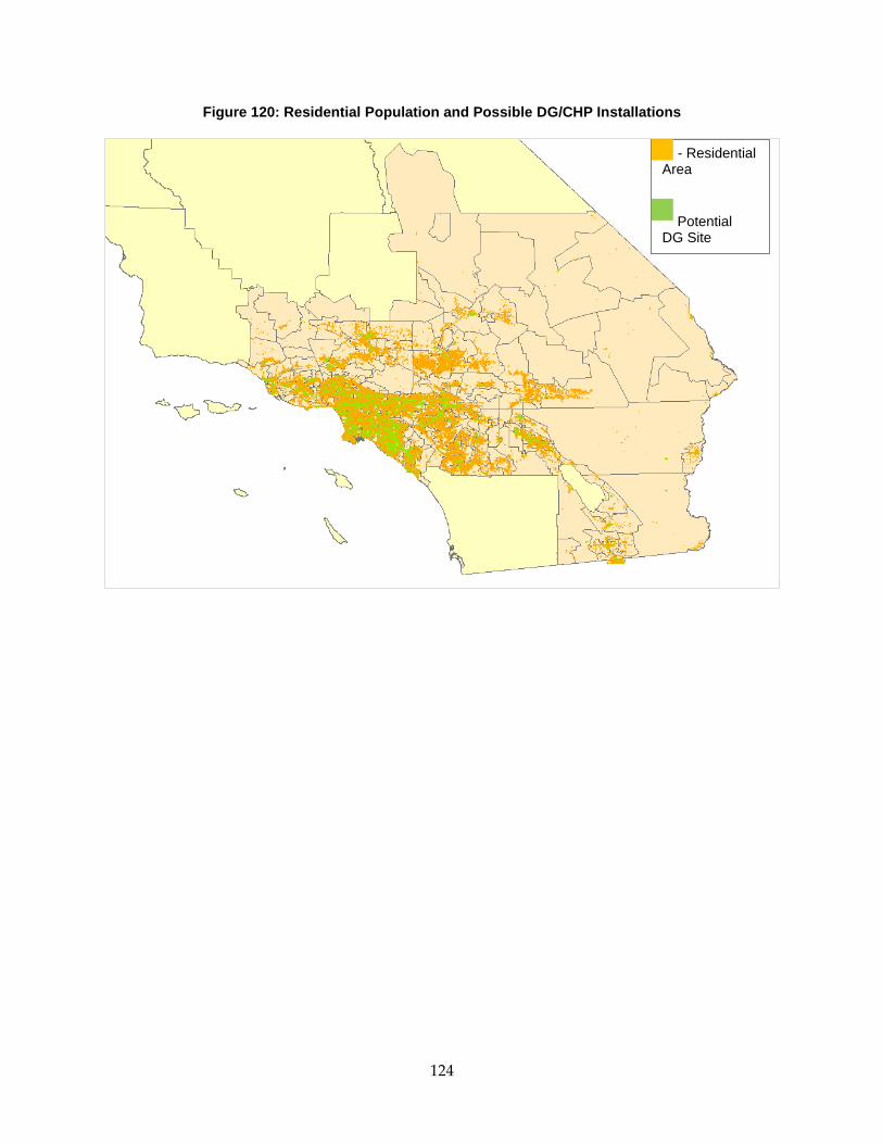
Figure 120: Residential Population and Possible DG/CHP Installations
- Residential Area Potential DG Site
124

Table 23: Potential Residential Population Impact of DG
Sector # in Region # Impacting Residential
Area
Night time Daytime
Max 6pm-6 am 6 am-6 pm
Commercial Office
1 – 10 stories 7272 403,171 0 201,585
11-40 stories 319 88,429 0 44,215
40+ stories 7 3,493 0 1,746
Hotels 1413 598 142,970 142,970 71,485
Hospitals 388 330 89,424 89,424 44,712
College/University 655 296 89,161 89,161 44,580
Jail/Prison 156 57 4,850 4,850 2,425
Totals ~326,400 ~410,750
% Population affected (17.9
million for region)
1.8% 2.2%
6.3.4 Summary The relative exposure analysis effort and results must be considered in the context of the data and the assumptions necessary at this level of study:
• A buffer zone was defined as 100 meters even though the plume modeling effort suggested that mixing and dilution of the exhaust plume to 1 percent of the exit plane levels occurred within 100 ft.
• Meteorological conditions (e.g. wind velocity, wind direction, and ground mixing) are not included. All residents that intersect with the buffer zone are included in the “affected” population
• The size, distribution, and orientation of the building(s) comprising the facility and the immediate surroundings are not included.
• The stack height of the DG is assumed to be at approximately 8 ft (as used in ground level plume modeling).
• The daytime residential density distribution is not known
125

• The Commercial Office building sector includes all office structures rather than limiting itself to “large commercial” as was identified in the study as the appropriate sector.
• The location of the DG/CHP system with a “facility” is not considered but rather is assumed to be at the facility boundary and the 100 meter buffer is established uniformly around the boundary of the facility. In reality, the DG is a point source located within the facility (at some location to be determined on a site by site basis) ; the 100 meter buffer zone would then be established from the point source
As such, the values provided are expected to significantly over-estimate the affected population. Additionally, recall that the plume is diluted within the 100 meter distance to levels comparable to the ambient air quality standards; hence even if the plume does interact with a population base within the 100 meters, the exposure to pollutant levels exceeding the ambient air quality standards is predicated on the existing air quality. Finally, the effect of exhaust stack height was not addressed. Extending the height of the exhaust stack could have significant impact on the dispersion of the plume and the definition of the buffer zone. At the extreme, if a DG/CHP system was located on the roof of a multi-floor building (11+ floor office building), it is highly unlikely that the plume effect would ever reach the residential areas in the immediate surroundings.
126
CHAPTER 7: Conclusions and Recommendations This program addressed the identification of business sectors that would likely benefit the most from the application of DG/CHP through the maximization of the generating on-site electric power while providing support of on-site thermal loads, both high temperature for heating and steam and low temperature such as cooling through the application of absorption chillers and similar systems) that could be met with waste heat recovery were included in the study. Beyond the identification, this program instrumented and monitored both the electric and thermal loads at participating facilities at nominally 15 minute intervals for extended period of time (roughly 12 months, some less, many more) to provide long term, temporally and seasonally resolved load profiles that provide a more detailed and parameter inter-related basis for assessing the application of DG/CHP systems for these sectors as opposed to yearly “averages” that do not show the range of variations nor any electric and heat load interaction. Finally, this program provided a basis for assessing the “near-field” impacts to occupants from exposure to DG/CHP exhaust for using plume modeling and GIS population/business information.
The breadth of the study and the conclusions derived are presented herein in a bullet format to help identify and emphasize the observations and analysis of the results.
1) All of the sectors analyzed could benefit from the application of DG/CHP. While this may seem self-evident given the sector evaluation and selection process, the decisions for the chosen sectors was based upon prima fascia annual energy data but no specific temporally resolved data on the typical energy loads and sub-loads for each sector to support this conclusion.
2) The specific DG system varies from sector to sector based upon the heat load needs versus the electric power needs. The following are identified based upon overall facility energy needs and implementation of DG to meet the overall needs. If a subset of the overall energy needs are to be met with DG, virtually any system can be successfully employed:
a. Food and Grocery:
i. The energy intensity of food/grocery facilities and the 24/7 operation make this sector a good fit.
ii. For applications today, the electric to thermal properties of a fuel cell (phosphoric acid or molten carbonate) would be a very good fit for on- site power and the use of waste heat to off-set sub-cooling and HVAC loads. This would result in nominal reductions of grid imports of 52 percent owing to on site generation and offsetting grid power needs for sub-cooling.
iii. For applications in the “future”, the electric to thermal properties of a reciprocating engine would be a very good fit for on-site power and the use of
127

waste heat to offset medium temperature chilling, sub-cooling and HVAC loads. This would result in nominal reductions of grid imports of 90+ percent owing to on site generation and offsetting grid power needs for sub-cooling, medium temperature and HVAC loads.
iv. The “future” application requires the development and deployment of lower temperature thermally activated cooling systems (e.g. ammonia based absorption chillers) that can support temperatures of nominally 20 deg F as well as the application of secondary cooling systems in the stores. The latter is best addressed at the time of the store construction as it requires the addition of liquid cooling systems to support refrigeration cases that would typically be installed in the foundation.
v. Low temperature cooling (< 0 deg F) will invariably need to be addressed through conventional vapor compression refrigeration cycles.
vi. The crucial need for refrigeration at food and grocery stores suggest that a refrigeration back-up system would be necessary if absorption chillers were installed in grocery/food application. This could be in the form of a back-up electric chiller powered by either the grid or the on-site DG, should the absorption chiller and/or the DG prime mover fail. Alternately the absorption chiller could incorporate an auxiliary burner for the absorption chiller to provide a heat source for the chiller should the DG prime mover fail. Currently, the redundancy of existing electric refrigeration systems at food and grocery facilities allows for one of more compressors to be out of service at a time and still meet cooling needs. It is unclear if multiple absorption chillers would be a practical alternative providing the same level of redundancy possible with a combination of electric chillers and back-up electric generation.
vii. Subcooling provides an efficiency gain for the facility but not crucial for the operation. Hence, subcooling system interruptions can be tolerated.
viii. Despite the potential for tremendous savings in electric grid imports (Figure 11), the critical nature of food refrigeration will likely result in the retention of electric vapor compression systems for chilling load and DG/CHP system applications limited to on-site power and sub-cooling.
b. Hotels:
i. Hotels have heating and cooling loads conducive to DG/CHP including large kitchen, laundry, pool/spa, and building heating and cooling needs.
ii. Gas turbines are optimal technology based upon the measured heat and electric needs.
iii. Reciprocating engines would be attractive if excess electric power could be placed back on the grid.
128

c. Commercial Office:
i. Gas turbines are the optimal technology based upon the measured heat and electric needs to support both heating and chilling needs.
ii. Reciprocating engines would be attractive if excess electric power could be placed back on grid
iii. The occupancy loading for commercial office (M-F, 6 am – 6pm) fits well with a peak shaving type application but requires a system that could be cycled on-off daily. As such, fuel cells would not be a good fit for commercial office facilities.
iv. Facilities that incorporate on-site energy storage (electrical and/or thermal) could benefit from 24/7 operation of a smaller system.
d. Colleges/University:
i. Gas turbines are the optimal technology based upon the measured heat and electric needs to support both heating and chilling needs as well as additional loads in the form of process steam. The large scale opportunities warrant the possibility of a large scale co-gen system capable of flexible support of heating, chilling, and additional electric generation as needed.
e. Hospitals:
i. Reciprocating engines are the optimal technology based upon the measured heat and electric needs.
ii. Gas turbines would be a good fit with some potential loss in efficiency. The large scale opportunities warrant the possibility of a large scale co-gen system capable of flexible support of heating, chilling, and additional electric generation as needed (as demonstrated with the UCDMC installation).
f. Jail/Prison:
i. All of the State prisons identified in the program do not have significant HVAC loads for prison population.
ii. Fuel cells (phosphoric acid and molten carbonate) are the optimal technology based upon current heat load to electric load measurements. Fuel Cell applications in this sector have already been demonstrated at some facilities (Santa Rita) but cost and payback are very long.
iii. If a move to air conditioned prison population is made, gas turbines would be the best match for heat and electric loads.
129

3) Barriers to adoption of DG/CHP include:
a. Perception that fuel cells especially and to some extent gas turbines are too exotic and too costly. Reluctance to invest in “cutting edge” or “bleeding edge” technology.
b. Reciprocating engines are accepted and understood; a comfortable solution. However, no reciprocating engine has been CARB certified. Deployment in areas is predicated upon local air quality rules and permitting issues. Air quality rules in SoCAB require permits for engines greater than 50 hp (35 kW) and annual emission testing.
c. Payback for the outright purchase or ownership of DG/CHP system is often too long for the “business” applications (food/grocery, commercial office, even hotels which tend to have longer acceptable payback) to invest in system
i. As a means of circumventing the upfront costs and the long payback periods, the emergence of Third Party Providers/ESCO’s and power purchase agreements are providing viable alternative to ownership for low/no capital outlay options.
d. Food and grocery has an entrenched “bias” towards fluorocarbon based electric refrigeration systems due to the need for high reliability and historical familiarity. Application of DG with thermally activated cooling would require substantial change to system configurations.
i. Most immediate application for DG/CHP is thermally activated cooling for sub-cooling and HVAC wherein existing lithium bromide based absorption chillers could be utilized.
ii. Medium temperature applications (e.g. meat case, dairy, deli) would require implementation of both ammonia based absorption chillers (to provide temps in the 20 F range necessary) and secondary fluid cooling loops (circulation of a fluid to the affected cases). The former exist but have very limited application to date while the latter requires extensive site modifications to incorporate (although it is being utilized in an effort to reduce the quantity of fluorocarbons at grocery stores).
iii. Implementation is better suited to new construction than to retrofit applications.
e. Colleges/Universities are slowly adopting the technology and applications (UCI, UCSD, CSUN, PCC, etc.). Rapid payback is not as great an issue since the facility and overall institution are not a volatile entity compared to a for profit business. Since public facilities are not able to capitalize upon any tax credit opportunities; many have opted for ESCO/PPA type of deployment opportunities.
130

f. Hospitals are slow to adopt DG/CHP technologies likely due to:
i. Need for power reliability. DG can actually increase reliability when combined with grid but economics do not favor 24/7 generation and there is concern DG/grid transitions will result in loss of power.
ii. The added scrutiny and perceived hindrance of State OSHPD oversight and approval of system installations.
g. Cost to generate versus electric utility rates typically favors peak use only. However, many of the larger systems that would be employed (large turbines, fuel cells) do not want to be cycled. As such, operation in non-peak periods can result in break-even or negative cash flow for low cost periods. This is highly dependent upon the spark spread between natural gas and electric power.
h. Current operational policy from local utilities (both IOUs and Municipal Utilities) generally prohibits net electric generation in excess of the site needs from crossing the site electric meter and entering the grid. A limitation on system sizing owing to the prohibition of back feeding to the grid creates issues relative to optimizing the overall system thermal efficiency and/or from addressing all of the site electric and thermal needs. Typical system design for maximum thermal efficiency would have all of the thermal needs addressed by the DG/CHP system (as the waste heat comprises the majority of the fuel energy) and consider that electricity as a beneficial by production. However, a no net generation/no back feeding directive in many cases results in a reduction of the available waste heat to meet the site thermal loads.
i. In all cases, the heat and electric loads could be met by one of the three predominant DG systems: fuel cell, reciprocating engines, and/or gas turbines.
ii. Allowing back feeding to the grid could allow the identification of more cost effective solutions that would otherwise not be a good heat to electric power match
iii. A Feed-In-Tariff does provide flexibility in sizing and cost effective design.
iv. It is expected that both the flexibility and the modicum of financial compensation provided by a Feed-In-Tariff will be beneficial to the deployment.
4) Enabling Technology Developments:
Observation of the 54 sites in this study and discussions with the facilities workers/managers associated with these facilities yielded information that would enhance the ability of DG/CHP systems to be deployed in an efficient manner. These include:
a. Hydronic based building systems are suitable for implementation of DG/CHP with thermally activated cooling. However, retrofit of a facility that utilizes direct expansion air conditioning (e.g. “Roof Top Units”) is not likely economically viable.
131
b. Simplified retrofit hydronic chilling systems that could readily fit within existing direct expansion air condition duct work. This would facilitate a shift towards hydronic systems and permit the application of absorption chilling.
c. Building systems that allow for on-site energy storage of both electric power and thermal energy (hot and/or cold) would be beneficial for highest efficiency 24/7 operation of system and allow for site to save generated energy for use during periods when it is more valuable.
d. Building Energy Control systems that are optimized for the on-site system and energy storage.
e. Ammonia based absorption chillers that provide lower temperatures (e.g. ~20 deg-F) for application in food and grocery sector (including food warehousing)
f. Hydronic “secondary fluid” cooling systems for food and grocery to replace the standard direct expansion cooling cases for medium temperature refrigeration needs would be useful. Such standard systems would be difficult to retrofit in existing stores (existing refrigeration lines are buried in the foundations) but could be implemented in new store design and construction. Development and improvements in thermally activated cooling systems to support the medium temperature refrigeration applications are crucial to the potential for DG/CHP to provide the noted energy efficiency opportunities.
5) Enabling Policy:
Observation of the 54 sites in this study and discussions with the facilities workers/managers associated with these facilities yielded information on incentives that would enhance the ability of DG/CCHP systems to be deployed in an efficient manner. These include:
a. Economic incentives to push the deployment of DG/CHP systems appear to be a significant factor in businesses moving forward with such a system. Therefore, continuing the incentive policy is key for the success of future deployment efforts.
b. The development of a “Feed in Tariff” whereby excess electric power generated by the DG/CHP system could be placed back on the grid (currently not permitted by California utilities), rather than reduce system output, could improve DG/CHP economics if tariff rates are favorable.
c. Carbon credit markets, generated by virtue of the higher thermal efficiency of a DG/CHP system, and the subsequent valuation in a future of carbon limits will provide a positive cash flow opportunity for owners. The market details/process/ and credit value will all have unforeseeable (likely positive) effects on overall impact on the deployment of DG/CHP.
132

d. While not directly policy related, favorable spark spread (the relative cost of fuel energy versus grid energy) certainly promotes the application of DG/CHP by providing a greater savings of the generated electric energy as compared to purchasing the energy from the grid. Expectations for policy mandated increases in penetration of high cost renewable power will likely result in increased grid power costs and the potential of a higher spark spread. It is uncertain what policies or other factors may impact natural gas prices and the spark spread.
6) Experience with Application of DG/CHP
This program had the opportunity to assess the “success” of DG/CHP installation efforts. In the SoCAB, the current application of DG/CHP systems has been only moderately successful. In 2001 many microturbine systems (100+) were deployed within the SoCAB through a SCAQMD distribution program. The units were offered “free” to applicants. Since there was neither facility motivation nor defined “need”, many (but not all) of these systems immediately feel into disrepair and were taken out of service (free system with no specific need with no budget to repair the systems). This set a negative perception of DG/CHP that still seems to exist. This experience and the interactions with those facilities that do have successful DG/CHP systems leads to the following conclusions/observations:
a. The value to the host site of DG/CHP system installation’s output (both electric and thermal) directly relates to the system availability.
i. The site provides the necessary personnel/maintenance staff to maintain operation
ii. Critical applications seem to derive great “value” for maintaining the operation of the system both from utility savings and avoidance of litigation due to system failure.
b. Higher cost systems fair better with availability
i. The level of investment seems to be reflected in on-site support for maintenance and upkeep.
c. Systems that do not provide significant support of a facilities needs have lower availability
i. Without significant financial investment or benefit, the systems are easy to neglect and not budget for maintenance and upkeep.
7) Relative Exposure of Population to DG/CHP
The widespread deployment of DG/CHP will have impacts on both the basin wide air quality and “near field” air quality. This program investigated the impact of DG/CHP deployment at retail food/grocery facilities throughout the SoCAB air basin. To assess the near field impacts, modeling of the exhaust plume dispersion was performed to assess the pollutant concentration levels in the immediate vicinity of the DG system.
133
a. DG/CHP on basin wide air quality, wide spread deployment of DG/CHP at retail food/grocery stores could provide enough electric energy generation to remove one central power plant from the SoCAB. The net emission change due to the deployment of DG/CHP and the removal of a central power plant correspond to less than 0.1 percent of the total basin-wide emissions. However, the reduction of emissions produced by the power plant shutdown is concentrated in one point, whereas the increase in emissions from CHP installations is spread throughout a large area of the domain. As a result, the changes in basin-wide pollutant concentrations are noticeable.
b. The removal of the power plant produces a reduction in 8-hour average O3 and in 24-hour average PM2.5 of 3 ppb and 1 µg/m3, respectively, in the proximity of the power plant. However, increases in 8-hour average O3 and in 24-hour average PM2.5 attributed to DG/CHP occur in areas around Riverside, and are of the order of 1 ppb and 1 µg/m3.
c. Exhaust plumes are mixed and diluted quickly with the ambient air. For an exhaust stack height of approximately 8 ft (typical of a microturbine installation), concentrations of exhaust pollutants are reduced two orders of magnitude within 100 meters of the point of exhaust.
d. Outside of the 100 meter radius of analysis, the impacts of diluted NOx pollutant levels for combustion based DG systems that meet CARB certification standards are diluted to a level one order of magnitude less than the ambient air quality standards.
e. Within the 100 meter radius of analysis and with an 8 ft exhaust height, the near source impacts of the diluted NOx pollutant emission for combustion based DG systems that meet CARB certification standards (after the lofted plume has mixed and returned to an elevation of 5 ft) are on the same order of magnitude of but less than the ambient air quality standards. As such, the pollutant concentrations from dispersed exhaust emissions as modeled from the DG/CHP system itself do not exceed the AAQS. However, it is possible, dependent upon the existing near field air quality, for the DG/CHP system to add to the background levels and cause the immediate area to exceed the ambient air quality standard.
f. Stack height does have a significant effect on the mixing and point of impact of the plume.
g. The reductions in emissions from equipment offset by waste heat recovery (i.e. boilers/furnaces, hot water heaters) are a benefit to local air quality and the impact of the DG/CHP and must be considered relative to the emissions from the source. The levels of offset vary from region to region dependent upon the local standards for the equipment and sizes. It is not possible to universally quantify
134

the impact of DG/CHP emissions against the reductions in emissions from displaced equipment.
h. Application of DG/CHP to all of the sectors outlined in the program in the South Coast Air Basin, on average, could affect 2 percent of the population through possible impacts on local air quality as defined by the 100 meter radius from the DG system.
135

GLOSSARY Term Definition
AAQS Ambient Air Quality Standard
AC Air Conditioning
ACLU American Civil Liberties Union
AES American Energy Services (energy provider)
AIS Aerial Information Systems, Inc.
AQMD (South Coast) Air Quality Management District
ASHRAE American Society of Heating, Refrigeration, and Air-conditioning Engineers
ASERTTI Association of State Energy Research and Technology Transfer Institutions
BACT Best Available Control Technology
BTU British Thermal Unity
CACM Cal-Tech Atmospheric Chemical Mechanism
CARB California Air Resources Board
CHP Combined Heat and Power
CEC California Energy Commission
CEUS Commercial End Use Survey
CFD Computational Fluid Dynamics
CHP Combined Heat and Power
CIEE California Institute for Energy and the Environment
COP Coefficient of Performance
CO Carbon Monoxide
CP Central Power (plant)
CSUN California State University Northridge
DER Distributed Energy Resource
DER-CAM Distributed Energy Resource Customer Adoption Model
DG Distributed Generation
136

DHW Domestic Hot Water
DX Direct Expansion (type of air conditioner utilizing Freon))
EEA Energy and Environmental Associates
EF Emissions Factor
EMI Electromagnetic Interference
EMS Energy Management System
ESCO Energy Service Companies
FEMP Federal Energy Management Program
EPA Environmental Protection Agency
FW Full Wall
GIS Geographic Information System
GWh (GW-hr) Gigawatt hour (= 1,000,000 kWh)
HHV Higher Heating Value
HRSG Heat Recovery Steam Generator
HT High Temperature (refrigeration) >20 F
HVAC Heating, Ventilation, Air Conditioning
HW Half Wall
ICE Internal Combustion Engine (reciprocating engine)
IP Internet Protocol
kWh (kw-hr) Kilowatt hour (unit of energy)
LACCD Los Angeles Community College District
LA-ISD Los Angeles Internal Services Department
LHV Lower Heating Value
LT Low Temperature (refrigeration) < 20 F
MCFC Molten Carbonate Fuel Cell
MMBtu Million Btu (British Thermal Unit)
MT Metric Ton
137

MTG Microturbine Generator
MWc Megawatt - cooling
MWe Megawatt - electricity
MWh (MW-hr) Megawatt hour ( = 1000 kWh)
NOx Oxides of Nitrogen
O3 Ozone
OSHA Occupational Safety and Health Administration
OSHPD Office of Statewide Health Planning and Development
PIER Public Interest Energy Research
PCC Pasadena City College
PM2.5 Particulate Matter less than 2.5 microns in size
PM10 Particulate Matter less than 10 microns in size
PV Photovoltaic
RANS Reynolds Averaged Navier Stokes
RD&D Research, Development, and Demonstration
RT Refrigeration Ton (= 12,000 Btu/hr)
RTD Resistance Temperature Devise
SCAGLU Southern California Association of Governments Land Use
SCAQMD South Coast Air Quality Management District
SCAQS Southern California Air Quality Study
SCE Southern California Edison (utility)
SGIP Self-Generation Incentive Program
SMUD Sacramento Municipal Utility District
SoCAB South Coast Air Basin
SO2 Sulfur Dioxide
SQL Structured Query Language
T-SQL Transact Structured Query Language
138

TCP Transmission Control Protocol
TIGER Topological Integrated Geographic Encoding and Referencing
TOU-GS Time of Use – General Services (utility rate)
UCDMC University of California Davis Medical Center
UCI-APEP University of California, Irvine – Advanced Power and Energy Program
UCI-CIT University of California Irvine – California Institute of Technology
UCSD University of San Diego
VA Veteran’s Administration
VOC Volatile Organic Compounds
139

REFERENCES
April 2005; prepared for the California Energy Commission by the Electric Power Research Institute (EPRI) and Energy and Environmental Associates (EEA); Report Number CEC-500-2005-060-D
Association of State Energy Research and Technology Transfer Institutions; 455 Science Dr, Ste 200, Madison WI, 53711
Campbell Scientific Inc., Logan UT; www.campbellsci.com
Dent Meter, Bend OR; www.dentinstruments.com
DOE, Quick Energy Simulation Tool (available at http://www.doe2.com/equest/) accessed 10 January 2006.
EEA, National Account Sector Energy Profiles 2003
Engineering Measurements Co., Longmont CO; www.emcoflow.us
Flex-Core, Milliard, OH; www.flex-core.com
FLUENT 6.3 Documentation
Griffin, R.J., Dabdub, D., Seinfeld, J.H., 2002a. Secondary organic aerosol. 1. Atmospheric chemical mechanism for production of molecular constituents. Journal of Geophysical Research 107(D17), 4332.
ITRON Inc., California Commercial End Use Survey, March 2006; prepared for the California Energy Commission by Itron Inc, Report Number CEC-400-2006-005
ITRON Inc., California Commercial End Use Survey, March 2006; prepared for the California Energy Commission by Itron Inc, Report NumberCEC-400-2006-005
ITRON Inc., California Commercial End Use Survey, March 2006; prepared for the California Energy Commission by Itron Inc, Report NumberCEC-400-2006-005
J.E. Bardina, P.G. Huang, and T.J. Coakley, 1997, ” Turbulence modeling validation, testing, and development”, NASA TM 110446.
Kay, Martin. 2006. Emissions from In-use IC Engine DG & Lessons Learned. SCAQMD. October 3,2006. www.energy.ca.gov/pier/conferences+seminars/2006-10-3+4_electricity_air-quality_conference/presentations/session_02/12Kay.ppt.
Mueller, Marla, Mark Wilson, Nicole Davis, Ed Vine, Jim Lents, Jan Sharpless. 2008. Impacts of Distributed Generation on Air Quality: A Roadmap. California Energy Commission, PIER Energy-Related Environmental Research Program. CEC-500-2008-022.
ONSITE SYCOM, Market Assessment of Combined Heat and Power Market in California, Energy Corporation, December 22, 1999
140

Sage Metering Inc, Monterey CA; www.sagemetering.com
SCE, California Self Generation Incentive Program Data Base: www.sce.com/RebatesandSavings/SelfGenerationIncentiveProgram
Siddiqui, A., Firestone, R., Ghosh, S., Stadler, M., Edwards, J., and Marnay, C. (2003). Distributed Energy Resource Customer Adoption Modeling with Combined Heat and Power Applications.
The Combined Heat and Power Database, EEA, 2005 http://www.eea-inc.com/testchp/index.html
The Market and Technical Potential for Combined Heat and Power in the Commercial/Institutional Sector, ONSITE SYCOM Energy Corporation, January 2000
Web link: http://www.census.gov/geo/www/tiger/overview.htm
Y. Xiao and H.W. Tang, 2006, “Numerical simulation of a horizontal momentum jet in cross-flow”, J. Hydrodynamics, Vol 18, pp. 118-125.
141

B-1