real effective exchange rate, broad money supply and trade

International Journal of Innovation, Creativity and Change. www.ijicc.net Volume 14, Issue 2, 2020

733

Real Effective Exchange Rate, Broad Money Supply, and Trade Balance in Vietnam: An Empirical Analysis from Bounds Test to a Cointegration Approach

Le Kieu Oanh Daoa, Van Chien Nguyenb*, Si Tri Nhan Dinhc, aBanking University of Ho Chi Minh City, Vietnam, bThu Dau Mot University, Vietnam, cSi Tri Nhan Dinh, Lam Dong province, Vietnam, Email: b*[email protected]

Objectives: This paper aims to investigate the impact of the real effective exchange rate and broad money supply on the trade balance in Vietnam using quarterly data from the first quarter of 2000 to the fourth quarter of 2018. Methods/ Statistical analysis: Using the ARDL-ECM approach to investigate this effect, a cointegration relationship exists between real effective exchange rate, broad money supply and trade balance. Findings: Results demonstrate that real effective exchange rate has a short-term negative impact on trade balance. Additionally, broad money supply has a positive impact on trade balance in the short run and long run with a very weak effect. Surprisingly, it was found that real foreign income and local income have no impact on trade balance.

Keywords: Exchange rate, broad money supply, trade balance, ARDL-ECM. JEL Classification Code: E43, E44, F31, F62, G18

Introduction Vietnam's economy is growing strongly and integrating deeply into the world economy with the trade balance being improved recently after a long period of deficit, bad debts in the banking system, and instable economic policies including the exchange rate policy (Nguyen and Do, 2020; Dao et al., 2020). In this case, the question "is the current exchange rate

http://www.ijicc.net/

mailto:[email protected]


734

suitable?” poses a problem that needs to be carefully discussed and planned for Vietnam. This is not only because the exchange rate policy must support export and import, but also because other significant macroeconomic variables have a large impact to Vietnam's economy along with income growth (GDP), basic interest rates, inflation, etc. (Le and Ishida, 2016; Nguyet et al. 2017; Nguyen and Do, 2020). In the context of the current world economy and Vietnam’s economy, there is an opinion to support the action of appreciating the Vietnam Dong (VND) compared to other currencies. In other words, the VND has depreciated because when the VND depreciates, the price of Vietnam's exports will be relatively cheaper than other countries, so exports will increase. However, according to other views, the depreciation of VND does not necessarily solve the problem of trade balance or will put pressure on commodity prices, inflation, capital inflows, etc. Although there have been many empirical studies and policy making reports, the discussion on how changes in exchange rates will improve the trade balance (Le and Ishida, 2016; Nguyen et al., 2017; Tran et al, 2020). However, there is still much disagreement about how the effect of exchange rate adjustments has an impact on the trade balance. In addition, assessing the relationship with the impact of exchange rates with the trade balance should be studied to provide a new perspective. In the study of Le and Ishida (2016), the devaluation of the Vietnamese currency in the long term will have a positive impact on the improvement of the trade balance with the research partners in the period 1990 - 2013. As suggested in a recent study by Nguyen et al. (2017), this research indicates that devaluation of the Vietnamese currency will worsen the trade balance in the period 2000-2015. There has been no empirical study on the relationship between exchange rate and trade balance in Vietnam in recent years, in particular to testing the J curve phenomenon in the country. Therefore, this study takes into account the previous research outlined above and continues to build upon this research in order to assess the effects of real effective exchange rate on Vietnam's trade balance in the short and long term. This research project will also assess whether volatility of the local currency can help improve the trade balance. The research objectives are to analyse this relationship in the short and long term in the period 2000 - 2018. Further, this research will discuss how the growth of money supply affects Vietnam's trade balance in the research period. The remainder of the paper is organised as follows. In the next section, the study will discuss the theoretical framework and review the existing literature. Then the researchers will present the research model, variables, and data collection methods used in the study. Finally, the researchers will present the main results which will be followed by a discussion and conclusion.



735

Theoretical Framework Referring to the studies of factors affecting trade balance, there have many types of research in terms of both theoretical and empirical. Theoretically, a country's economic transactions with an open economy are reflected in its balance of payments. The exchange rate exists in a close relationship with the balance of payments as well as the with the balance of payments components such as the trade account in the current account (Koivu and García-Herrero, 2007; Nguyen and Do, 2020; Hussain and Hassan, 2020; Hussain et al., 2020; Kamran et al., 2020). Numerous studies have given many theoretical frameworks related to trade balance in the world. This includes the theories of Le and Ishida (2016); Nguyen et al. (2017); Tran et al. (2020), Mukherjee et al. (2020). Through the research, the following approaches are established: elasticity approach, absorption approach and monetary approach. Elasticity Approach and Marshall-Lerner Condition As observed in the previous study, Bickerdike – Robinson – Metzler condition (BRM condition) is the initial theoretical foundation for the elasticity approach. This approach was established by the research of by Bickerdike (1920) and later, Robinson (1947) and Metzler (1948) continue to contribute to the elasticity method by clarifying and detailing Bickerdike's ideas. As shown by Marshall-Lenner condition, which was developed by Marshall (1923), Lerner (1944) and the theory of J-curve curve effects of the relationship between exchange rate and trade balance, further developed and extended this argument. In addition, Marshall-Lerner condition is a further extension of Bickerdike – Robinson – Metzler condition. The most studies discuss that trade balance is defined as exports minus imports, thus: 𝑇𝑇𝑇𝑇 = 𝑋𝑋 −𝑀𝑀 = 𝑋𝑋 − 𝑆𝑆𝑀𝑀∗ (1) M * is the import value in foreign currency price, in contrast to M, the import price in local currency price. Accordingly, M = SM *, when S is the exchange rate, then equation above is transformed as follows: 𝑑𝑑𝑑𝑑𝑑𝑑𝑑𝑑𝑑𝑑

= 𝑑𝑑𝑑𝑑𝑑𝑑𝑑𝑑− 𝑆𝑆 𝑑𝑑𝑀𝑀∗

𝑑𝑑𝑑𝑑− 𝑀𝑀∗ (2)

And after rearranging equation (2), we have the following relationship: 𝑑𝑑𝑑𝑑𝑑𝑑𝑑𝑑𝑑𝑑

= 𝑑𝑑𝑑𝑑𝑑𝑑𝑑𝑑 𝑑𝑑⁄𝑑𝑑𝑑𝑑 𝑑𝑑⁄

− 𝑀𝑀∗ 𝑑𝑑𝑀𝑀∗ 𝑀𝑀∗⁄

𝑑𝑑𝑑𝑑 𝑑𝑑⁄− 𝑀𝑀∗ = 𝑑𝑑

𝑑𝑑𝐸𝐸𝑑𝑑 + 𝑀𝑀∗𝐸𝐸𝑀𝑀 −𝑀𝑀∗ = 𝑀𝑀∗ � 𝑑𝑑

𝑑𝑑𝑀𝑀∗ 𝐸𝐸𝑥𝑥 + 𝐸𝐸𝑀𝑀 − 1� (3)

When 𝐸𝐸𝑑𝑑 = 𝑑𝑑𝑑𝑑 𝑑𝑑⁄𝑑𝑑𝑑𝑑/𝑑𝑑

and 𝐸𝐸𝑀𝑀 = 𝑑𝑑𝑀𝑀∗ 𝑑𝑑𝑀𝑀∗⁄𝑑𝑑𝑑𝑑/𝑑𝑑

are the elasticity of exports and imports, with both

added the function of exchange rates. This demonstrates exports almost increasing and



736

imports almost decreasing when the exchange rate rises, or the local currency depreciates. Further, assuming the initial equilibrium transaction i.e. X = SM * at the beginning of the analysis, then, equation (3) becomes: 𝑑𝑑𝑑𝑑𝑑𝑑𝑑𝑑𝑑𝑑

= 𝑀𝑀∗(𝐸𝐸𝑑𝑑 + 𝐸𝐸𝑀𝑀 − 1) (4) It is important to note that Equation (4) is a Marshall - Lerner condition, stating that domestic currency devaluation leads to an improvement in the domestic trade balance of the country, which is conditional on the sum of export and import elasticities. Its exports are larger than one unit. Therefore, trade balance worsens after the devaluation of the local currency if the country's total export and import elasticity is lower than one unit (Wang, 2009). If EX and EM represent for export elasticity and import elasticity, we express the Marshall-Lerner condition as an expression: EX + EM > 1 (in case of improved trade balance) and EX + EM <1 (in case of declined trade balance) J Curve Phenomenon Following the approach in macroeconomics (Marshall, 1923; Lerner, 1947; Robinson, 1947; Metzler, 1948), J curve reflects the devaluation of the national exchange rate affecting the trade balance over time (Robinson, 1947; Metzler, 1948). Theoretically, in the short-term, shortly after the devaluation of the currency, domestic importers face rising import prices when they pay for goods in the local currency. Therefore, net exports decreased. On the other hand, domestic exporters face lower export prices due to the relatively inelastic demand of export and import in the short term. The non-elasticity of this demand is caused by a slowdown in changing consumer behaviour and the delay of renegotiation agreements. In other words, in the short run when prices are relatively stable, trade balance faces a decline due to the stickiness of prices and the sluggishness in changing demand. The assumption is when the goods are still traded at the price before devaluation. Therefore, trade balance is worsened by the value of total imports in foreign currencies multiplied by the increase in the price of foreign currencies since the contracts were performed before depreciation forced prices and fixed volumes. The short-term period is often referred to as the period of “exchange rate pass-through”. Subsequently, domestic demand began to shift from abroad to domestic production of substitutes as a response to higher import prices, resulting in an improvement in the trade balance. Numerous empirical studies have demonstrated that the J curve phenomenon predicts that trade balance will improve in the long run to a level higher than its pre-depreciation level (Bahmani-Oskooee, 1985; Melvin and Norrbin, 2012). The dynamic reaction of the trade



737

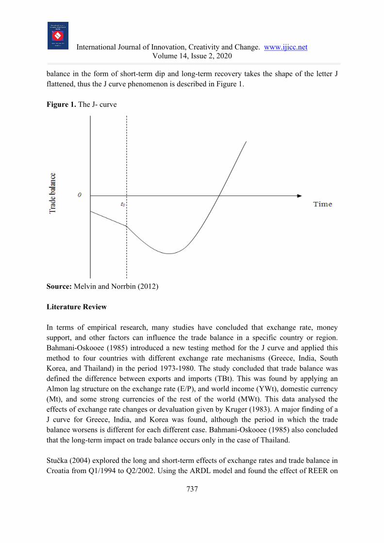
balance in the form of short-term dip and long-term recovery takes the shape of the letter J flattened, thus the J curve phenomenon is described in Figure 1. Figure 1. The J- curve

Source: Melvin and Norrbin (2012) Literature Review In terms of empirical research, many studies have concluded that exchange rate, money support, and other factors can influence the trade balance in a specific country or region. Bahmani-Oskooee (1985) introduced a new testing method for the J curve and applied this method to four countries with different exchange rate mechanisms (Greece, India, South Korea, and Thailand) in the period 1973-1980. The study concluded that trade balance was defined the difference between exports and imports (TBt). This was found by applying an Almon lag structure on the exchange rate (E/P), and world income (YWt), domestic currency (Mt), and some strong currencies of the rest of the world (MWt). This data analysed the effects of exchange rate changes or devaluation given by Kruger (1983). A major finding of a J curve for Greece, India, and Korea was found, although the period in which the trade balance worsens is different for each different case. Bahmani-Oskooee (1985) also concluded that the long-term impact on trade balance occurs only in the case of Thailand. Stučka (2004) explored the long and short-term effects of exchange rates and trade balance in Croatia from Q1/1994 to Q2/2002. Using the ARDL model and found the effect of REER on



738

the trade balance. At the same time, there exists a J curve effect in Croatia. Further investigated on a study in China by Koivu and García-Herrero (2007), trade balance is very sensitive to the volatility of REER and indicated that if the RMB (Yuan) are properly priced. It had a positive impact on China's trade surplus between 1994 and 2005. However, Wang et al. (2012) concluded that the appreciation of the Renminbi has no long-term impact on the balance of trade, while the appreciation has a significant short-term impact on research on the devaluation of China and its trading partners in the period 2005-2009. Kurtović (2017) studied Albanian the real effective exchange rate (REER) data and trade balance quarterly from 1994 to 2015, using VECM model and a co-integration test. The study's findings suggest that GDP has a positive effect on trade balance with a weak presence of J curve effect in the both long and short run. In addition, dumping will improve trade balance but will not work with an inappropriate macro policy. As suggested in Begović and Kreso (2017), the opposite conclusion could be found because devaluation of domestic currency would cause a decline in trade balance when they were analysing panel data for 2000-2015 period of transitioning economies in Europe (including: Albania, Bosnia & Herzegovina, Bulgaria, Cyprus, Croatia, Estonia, Greece, Hungary, Latvia, Lithuania, Macedonia, Poland, Romania, Serbia, Slovakia, Slovenia, Turkey). In a study in the US, Rose and Yellen (1989) investigated the presence of a J curve at a bilateral level during 1963-1988 for US quarter data by testing stationarity for time-series data and cointegration between variables. Rose and Yellen (1989) argued that bilateral analysis is useful because it does not require the construction of an income variable that represents the rest of the world and that it reduces the aggregate bias. With the same conclusion, Rose (1991) used the overall trade data of 5 major OECD countries, UK, Canada, Germany, Japan, and the USA to find the relationship between REER and trade balance. In addition, Bahmani-Oskooee and Kantipong (2001) studied Thailand and their 5 major trading partners by using ARDL model combined with quarterly data from 1973-1997. The model results only showed the existence of the J-curve effect in bilateral trade between Thailand and Japan and the US. Further discussed on trade balance, Yuen-Ling et al. (2009) determined the relationship between the real exchange rate and the trade balance of Malaysia from 1955 to 2006 with some conclusions as follows: (1) there exists a relationship which is a long-term relationship between the exchange rate and the trade balance, (2) devaluation of the local currency will improve the trade balance in the long term, (3) there is no J curve effect in the case of Malaysia. This conclusion contradicts Duasa's (2007) earlier study, where there was no long-term relationship between the exchange rate and the trade balance of Malaysia between 1974 and 2003. Similarly, Bahmani-Oskooee and Fariditavana (2015) also used bilateral trade data for this new method using the ARDL approach both linear and nonlinear. With the bilateral



739

trade data between the United States and the six major trading partners, namely Canada, France, Germany, Italy, Japan and the United Kingdom, when using the linear ARDL approach, they found evidence of the effects of the J curve for the trade model between USA and Canada, France and Germany. However, when the asymmetric ARDL approach was used, the J curve effect was discovered in five of the six models (except for the Japanese case). Bahmani-Oskooee et al. (2016) conducted a study in Mexico with their 13 trading partners, applying both linear and asymmetric methods with cointegration and error correction models, to test whether the impact of the devaluation of the peso on the trade balance is different from the impact of the peso appreciation. The linear ARDL model gives a long-term coefficient that is statistically significant for the six partners, which implies that while the fall in pesos improves Mexico's trade balance with these countries. The increase Price of pesos hurt their trade balance. However, the asymmetric ARDL model results showed that the appreciation and depreciation of the local currency have a significantly different effect on the trade balance. Indeed, while the depreciation of the peso improves the trade balance of Mexico with Brazil, Canada, France, Japan, Korea, Spain, and the UK, the appreciation of the peso worsens the trade balance. This includes trade in the case of Brazil, Canada, France, USA, India, Japan, Korea, Peru and Spain. Thus, the exchange rate change has an asymmetric effect on Mexico's bilateral trade balance. Table 1 demonstrates the results of all above discussions: Table 1: Brief Summaries of Previous Study Authors Analysis

method Independent variable

Results

Bahmani - Oskooee (1985)

Almon lag structure

Exchange rate; Income of the world and nation; Domestic and the rest of world strong money supply

Evidence of J curve in different cases Long-term impact only occurs in the case of Thailand

Rose & Yellen (1989)

Cointegration REER, U.S real GNP, GDP/GNP of foreign

No impact of exchange rates on trade balance Contribute to a method of separating trade data and establishing their relationship with exchange rates.

Rose (1991) Cointegration CPI, M1, Short-term interest,

Exchange rates have a significant effect on trade balance.



740

REER The Marshall - Lerner condition is still met.

Stučka (2004)

ARDL model REER based on CPI and PPI, Domestic and foreign GDP

Find the impact of REER on the trade balance Find evidence of J curve

Koivu & Garcia -Herrero (2007)

Cointegration Johansen

REER, Domestic and foreign needs, Controls

China's trade balance is sensitive because of fluctuations of REER Properly priced Yuan will have an impact on China's trade surplus.

Duasa (2007)

ARDL model Exchange rate; GDP; Money supply M3

There is no J curve effect Exchange rate has no effect on trade balance in long and short term. Income and money supply play an important role in affecting the trade balance in long term.

Yuen-Ling et al. (2009)

Cointegration Granger causality, VECM

Exchange rate; Malaysia and U.S GDP

A long-term relationship exists between the exchange rate and the trade balance. Devaluation of the local currency will improve the trade balance in the long run and have no J curve effect.

Wang et al. (2012)

Fully-modified OLS Panel ECM

Exchange rate and GDP

The appreciation of the renminbi has no long-term impact on the trade balance, while it has a significant short-term impact.

Shah and Majeed (2014)

ARDL model REER; Pakistan GDP; Money supply M2

Exchange rates, money supply and income play a major role in determining the long-term response of trade balance Devaluation has a negative effect in both short and long term on trade balance

Bahmani-Oskooee & Fariditavana (2015)

Linear and nonlinear ARDL model

Real exchange rate; U.S and trade partners ‘s income

The effect of exchange rates on the trade balance is asymmetric There appears a curve J; Introduction of non-linear ARDL



741

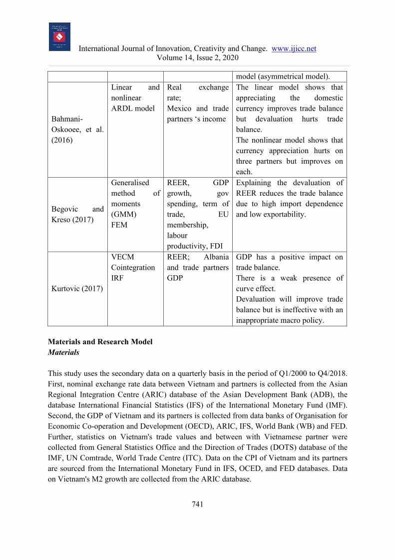
model (asymmetrical model).

Bahmani-Oskooee, et al. (2016)

Linear and nonlinear ARDL model

Real exchange rate; Mexico and trade partners ‘s income

The linear model shows that appreciating the domestic currency improves trade balance but devaluation hurts trade balance. The nonlinear model shows that currency appreciation hurts on three partners but improves on each.

Begovic and Kreso (2017)

Generalised method of moments (GMM) FEM

REER, GDP growth, gov spending, term of trade, EU membership, labour productivity, FDI

Explaining the devaluation of REER reduces the trade balance due to high import dependence and low exportability.

Kurtovic (2017)

VECM Cointegration IRF

REER; Albania and trade partners GDP

GDP has a positive impact on trade balance. There is a weak presence of curve effect. Devaluation will improve trade balance but is ineffective with an inappropriate macro policy.

Materials and Research Model Materials This study uses the secondary data on a quarterly basis in the period of Q1/2000 to Q4/2018. First, nominal exchange rate data between Vietnam and partners is collected from the Asian Regional Integration Centre (ARIC) database of the Asian Development Bank (ADB), the database International Financial Statistics (IFS) of the International Monetary Fund (IMF). Second, the GDP of Vietnam and its partners is collected from data banks of Organisation for Economic Co-operation and Development (OECD), ARIC, IFS, World Bank (WB) and FED. Further, statistics on Vietnam's trade values and between with Vietnamese partner were collected from General Statistics Office and the Direction of Trades (DOTS) database of the IMF, UN Comtrade, World Trade Centre (ITC). Data on the CPI of Vietnam and its partners are sourced from the International Monetary Fund in IFS, OCED, and FED databases. Data on Vietnam's M2 growth are collected from the ARIC database.



742

Nominal Effective Exchange Rate (NEER) and Real Effective Exchange Rate (REER) The calculation formula and data collection of real effective exchange rate are presented as follows: The study follows the base year of 2000 because of the following reasons: (1) The State Bank announced the change of Vietnam's exchange rate mechanism to float with regulated and nominal value of VND carried closer to real value in relation to other currencies; (2) It is easier to collect data since 2000. Thus, the quarter 1/2000 is selected as the base period used for calculation, due to the quarterly data used in the study. Further, currency basket and nominal exchange rate used for the study including the following currencies: the U.S Dollars (USD), Euro (EUR), Australian Dollar (AUD), Japanese Yen (JPY), Chinese Renminbi Yuan (CNY), Singapore Dollar (SDG), Thai Bath (THB), Malaysian Ringgit (MYR), Korean Won (KRW), Russian rouble (RUB), Indian Rupee (IRP), New Zealand Dollar (NZD), British Pound (GBP), Hongkong Dollar (HKD), Swiss franc (CHF), Canadian Dollar (CAD). CPI figures of the trading partners used in the study and of Vietnam, which is the CPI of this quarter compared with the same period of the previous year. The CPI of each country is adjusted to the base period. If the base period is Q1/2000, the CPI of the base period is 100, the adjusted CPI at time t is calculated by the following formula: 𝐶𝐶𝐶𝐶𝐶𝐶0𝑡𝑡 = 𝐶𝐶𝐶𝐶𝐶𝐶𝑡𝑡

𝐶𝐶𝐶𝐶𝐶𝐶0× 100 (5)

where CPI0t is the adjusted CPI at time t, CPIt is the actual CPI for period t, CPI0 is the actual CPI in the base period. Therefore, the formula for REER and NEER:

𝑹𝑹𝑹𝑹𝑹𝑹𝑹𝑹 = ∑ � 𝒆𝒆 𝒕𝒕𝒋𝒋

𝒆𝒆𝒃𝒃𝒃𝒃𝒃𝒃𝒆𝒆𝒋𝒋 . 𝑷𝑷𝒕𝒕

𝒋𝒋

𝑷𝑷𝒕𝒕𝑽𝑽𝑽𝑽� .𝒘𝒘𝒕𝒕

𝒋𝒋𝒏𝒏𝒊𝒊=𝟏𝟏 and 𝑽𝑽𝑹𝑹𝑹𝑹𝑹𝑹 = ∑ 𝒆𝒆𝒕𝒕

𝒋𝒋

𝒆𝒆𝒃𝒃𝒃𝒃𝒃𝒃𝒆𝒆𝒋𝒋 .𝒘𝒘𝒕𝒕

𝒋𝒋𝒏𝒏𝒊𝒊=𝟏𝟏 (6)

Which is NEER, REER are the nominal, real effective exchange rate of selected currencies ejt is the bilateral nominal exchange rate of the j currency against VND in period t ejbase is the bilateral nominal exchange rate of the currency of the jth country against VND in the base period wjt is the commercial proportion of j partner at time t PVNt is Vietnam's price index at time t. Pjt is the j partner price index at time t. i is the calculation period. j is the order of the countries selected in the currency basket



743

TB: is representative of Vietnam's trade balance, is the ratio of export value to import value calculated by the following formula: (X M⁄ )t = Xt

Mt with X, M respectively are export value

and import value in the t. GDPVN and GDPw: respectively the GDPVN growth rate of Vietnam and the GDPw growth rate are the average GDP index of trading partners. GDPw is calculated by the following formula: 𝐺𝐺𝐺𝐺𝐶𝐶𝑤𝑤 𝑡𝑡 = ∑ 𝐺𝐺𝐺𝐺𝐶𝐶𝑗𝑗𝑡𝑡 .𝑊𝑊𝑗𝑗

𝑡𝑡𝑛𝑛𝑗𝑗=1

M2: is Vietnam's M2 money growth, expressed as a percentage. Research Model Combining the theory of elasticity approach and monetary approach presented above, the research model used in the research topic is the empirical equation modelled as follows: 𝑇𝑇𝑇𝑇 = 𝑓𝑓(𝑅𝑅𝐸𝐸𝐸𝐸𝑅𝑅,𝐺𝐺𝐺𝐺𝐶𝐶𝑉𝑉𝑉𝑉 ,𝐺𝐺𝐺𝐺𝐶𝐶𝑤𝑤 ,𝑀𝑀2) = 𝛽𝛽0 + 𝛽𝛽1𝑅𝑅𝐸𝐸𝐸𝐸𝑅𝑅𝑡𝑡 + 𝛽𝛽2(𝐺𝐺𝐺𝐺𝐶𝐶𝑉𝑉𝑉𝑉)𝑡𝑡 + 𝛽𝛽3(𝐺𝐺𝐺𝐺𝐷𝐷𝑤𝑤)𝑡𝑡 + 𝛽𝛽4(𝑀𝑀2)𝑡𝑡 + 𝜀𝜀 (7) Or equation (7) written in natural logarithm

𝑙𝑙𝑙𝑙𝑇𝑇𝑇𝑇𝑡𝑡 = 𝛽𝛽0 + 𝛽𝛽1𝑙𝑙𝑙𝑙𝑅𝑅𝐸𝐸𝐸𝐸𝑅𝑅𝑡𝑡 + 𝛽𝛽2𝑙𝑙𝑙𝑙(𝐺𝐺𝐺𝐺𝐶𝐶𝑉𝑉𝑉𝑉)𝑡𝑡 + 𝛽𝛽3𝑙𝑙𝑙𝑙(𝐺𝐺𝐺𝐺𝐶𝐶𝑊𝑊)𝑡𝑡 + 𝛽𝛽4𝑙𝑙𝑙𝑙(𝑀𝑀2)𝑡𝑡 + 𝜀𝜀𝑡𝑡 (8) lnTBt represents the trade balance at period t in the form of a natural logarithm, defined as the ratio of the value of merchandise exports to the value of merchandise imports (X / M ratio). This calculation was chosen instead of the absolute value of trade balance because trade balance is the difference between the value of exports and the value of imports facing the weakness of being sensitive to the unit of measurement if possible present in natural logarithm. lnREERt represents the real effective exchange rate at period t as a natural logarithm. Wang (2009) argues that increasing or decreasing REER is equivalent to the appreciation or depreciation of the local currency against the foreign currency. Therefore, β1 is expected to be positive to improve the trade balance. lnGDPVN represents the real GDP growth index of Vietnam at the t period in the logarithm form and the lnGDPw is the real GDP growth index of the trading partner in the t period in the logarithm form. Further, β2 is expected to be negative, while β3 is expected to be positive because Vietnam's GDP increases, the demand for imported goods increases and vice versa. The GDP of trade partners will change and help to increase the demand for goods export.



744

lnM2 is the M2 growth rate of Vietnam at period t in the logarithm form. From the theory of money access, β4 is expected to be negative because as the money supply increases, it will worsen the trade balance. β0, β1, β2, β3, β4 are the regression coefficients εt is the random error at period t. Empirical Results Stationarity Test Table 2: Stationary Test

Variable Explanation t-Statistic Prob. Result

lnTB Trade balance -4.020542 At level 0.0022 Stationary at I(0)***

lnREER REER -5.730351 At first difference

0.0000 Stationary at I(1)***

lnGDPvn GDP of Vietnam -3.363621 At first difference

0.0158 Stationary at I(1)**

lnGDPw GDP of partners -5.986593 At level 0.0000 Stationary at I(0)***

lnM2 Broad money supply

-6.301238 At level

0.0000 Stationary at I(0)***

Note: I(0): level, I(1): first different (***), (**), (*) significance level at 1%, 5%, and 10% Source: Authors' calculations The results of the ADF test show that the variables used in the topic are stationary with I (0) or I (1), that is, all variables stop at the original series or stop at the first stationary. According to Table 2 above, the variables REER, Vietnam GDP all stop at the first stationary and the variables trade balance, partner GDP, M2 money supply stop at the level. Therefore, the ARDL model can be used to test the short- and long-term relationship between variables in the research model. Optimal Lag Length and Bounds Test To select the optimal lag length for the economic research model, according to Wooldridge (2013), the latency from 1 to 8 is consistent with quarterly data and for monthly data. The



745

latency can be 6, 12, or 24 when there is sufficient matching data. Thus, the optimal latency will correspond to the model with the smallest information standard value. For the ARDL model, we select the most optimal latency according to the Schwarts information standard (SIC) and select the optimal latency of 3. Table 3: Optimal Lag Length Selection with Unrestricted VAR

Lag LogL LR FPE AIC SIC HQ 0 512.565 NA 5.2e-13 -14.099 -14.0361 -13.9409

1 792.353 559.57 4.4e-16 -21.1765 -20.7988 -20.2279

2 861.275 137.84 1.3e-16 1.3e-16 -22.3965 -21.7042

3 898.913 75.277* 9.4e-17* -22.7476* -21.7405* -20.218

4 915.515 33.204 1.3e-16 -22.5143 -21.1926 -19.1942 Source: Authors' calculations Bounds test The null hypothesis: 𝛽𝛽0 = 𝛽𝛽1 = 𝛽𝛽2 = 𝛽𝛽3 = 𝛽𝛽4 The alternative hypothesis: 𝛽𝛽0 ≠ 𝛽𝛽1 ≠ 𝛽𝛽2 ≠ 𝛽𝛽3 ≠ 𝛽𝛽4 The estimated F-test statistics have a statistical value of 5.164 given in Table 4, exceeding the upper boundary limit of 5.06 at 5% significant level. This resulted in the conclusion that rejected the null hypothesis and argued that there was a long-term relation between variables. This means that four variables used in research topics move together in the long term. Table 4: F-statistic Test Results

k F-statistic Significance Significance Bounds value of F-statistic Lower-bound Upper-bound

4 5.164

10% 2.45 3.52 5% 2.86 4.01 2.5% 3.25 4.49 1% 3.74 5.06

Source: Authors' calculations To perform the bounds test for cointegration, the conditional ARDL (l, m, n, p, q) is specified as follows: ∆𝑙𝑙𝑙𝑙𝑇𝑇𝑇𝑇𝑡𝑡 = 𝛽𝛽0+𝛽𝛽1𝑙𝑙𝑙𝑙𝑅𝑅𝐸𝐸𝐸𝐸𝑅𝑅𝑡𝑡−𝑖𝑖 + 𝛽𝛽2𝑙𝑙𝑙𝑙(𝐺𝐺𝐺𝐺𝐶𝐶𝑉𝑉𝑉𝑉)𝑡𝑡−𝑖𝑖 + 𝛽𝛽3𝑙𝑙𝑙𝑙(𝐺𝐺𝐺𝐺𝐶𝐶𝑊𝑊)𝑡𝑡−𝑖𝑖 + 𝛽𝛽4𝑙𝑙𝑙𝑙(𝑀𝑀2)𝑡𝑡−𝑖𝑖 +∑ β1𝑗𝑗∆𝑙𝑙𝑙𝑙𝑇𝑇𝑇𝑇𝑡𝑡−𝑖𝑖𝑙𝑙𝑖𝑖=1 + ∑ 𝛾𝛾2j𝑚𝑚

𝑖𝑖=1 ∆𝑙𝑙𝑙𝑙𝑅𝑅𝐸𝐸𝐸𝐸𝑅𝑅𝑡𝑡−𝑖𝑖 + ∑ 𝛿𝛿3j∆𝑙𝑙𝑙𝑙(𝐺𝐺𝐺𝐺𝐶𝐶𝑉𝑉𝑉𝑉)𝑡𝑡−𝑖𝑖𝑛𝑛𝑖𝑖=1 +

∑ 𝜗𝜗4j𝑝𝑝𝑖𝑖=1 𝑙𝑙𝑙𝑙(𝐺𝐺𝐺𝐺𝐶𝐶𝑊𝑊)𝑡𝑡−𝑖𝑖 + ∑ 𝜃𝜃5𝑗𝑗

𝑞𝑞𝑖𝑖=1 𝑙𝑙𝑙𝑙(𝑀𝑀2)𝑡𝑡−𝑖𝑖 + 𝜀𝜀𝑡𝑡 (9)



746

Estimation results can be written as follows: ∆𝑙𝑙𝑙𝑙𝑇𝑇𝑇𝑇𝑡𝑡 = 𝛽𝛽0 + ∑ β1𝑖𝑖∆𝑙𝑙𝑙𝑙𝑇𝑇𝑇𝑇𝑡𝑡−𝑖𝑖𝑙𝑙

𝑖𝑖=1 + ∑ 𝛾𝛾2i𝑚𝑚𝑖𝑖=1 ∆𝑙𝑙𝑙𝑙𝑅𝑅𝐸𝐸𝐸𝐸𝑅𝑅𝑡𝑡−𝑖𝑖 + ∑ 𝛿𝛿3i∆𝑙𝑙𝑙𝑙(𝐺𝐺𝐺𝐺𝐶𝐶𝑉𝑉𝑉𝑉)𝑡𝑡−𝑖𝑖𝑛𝑛

𝑖𝑖=1 +∑ 𝜗𝜗4i𝑝𝑝𝑖𝑖=1 𝑙𝑙𝑙𝑙(𝐺𝐺𝐺𝐺𝐶𝐶𝑊𝑊)𝑡𝑡−𝑖𝑖 + ∑ 𝜃𝜃5𝑖𝑖

𝑞𝑞𝑖𝑖=1 𝑙𝑙𝑙𝑙(𝑀𝑀2)𝑡𝑡−𝑖𝑖 + λ.𝐸𝐸𝐶𝐶𝑇𝑇𝑡𝑡−1 + 𝜀𝜀𝑡𝑡 (10)

𝐸𝐸𝐶𝐶𝑇𝑇 = (𝑙𝑙𝑙𝑙𝑇𝑇𝑇𝑇𝑡𝑡−𝑖𝑖 − θ.𝑋𝑋𝑡𝑡) , the error correction term is the extracted residuals from the regression of the long-run equation. Which is: θ: long-run coefficient t: time l, m, n, p, q: lag lengths. In which, l, m, n, p, and q show the optimal latency of each related variable in the model and is determined by AIC or SIC information standards. Thus, the model can be of the form ARDL (l, m, n, p, q) and long-term correlation coefficients can be calculated when estimating the ARDL model (l, m, n, p, q). The results of the ARDL model (3,2,0,0,2) and the long-term correlation coefficients are shown in Table 5 below. Table 5: Estimation of Long and Short-term Coefficient in ARDL (3,2,0,0,2) Model

Variables Coefficient Std. Err. t-Statistic Prob.*

LnREER 0.1503833 .1282318 1.17 0.245

LnGDPVN -2.310835 2.393496 -0.97 0.338

LnGDPW 0.9874919 1.5968 0.62 0.539 LnM2 -0.1304639 .0738892 -1.77 0.082* ECMt-1 -0.4699124 0.1035544 -4.54 0.000*** ∆LnTB(-1) -0.2001994 0.1211777 -1.65 0.104 ∆LnTB(-2) 0.1336672 0.1161837 1.15 0.255 ∆LnREER 0.1282538 0.3918245 0.33 0.745 ∆LnREER(-1) -1.058506 0.4077515 -2.60 0.012** ∆LnGDPvn 1.409087 1.239126 1.14 0.260 ∆LnGDPw -1.244669 1.227334 -1.01 0.315 ∆LnM2 0.0906543 0.0575801 1.57 0.121 ∆LnM2(-1) -0.1047773 0.0637184 -1.64 0.095* _cons 2.80142 4.073579 0.69 0.494 R2 0.5786 Adjusted R2 0.5026 Root MSE 0.0691

Note: (***), (**), (*) are respectively 1%, 5%, and 10% significance level Source: Authors' calculations



747

The results can be explained that more than 57% of the long-term change from the variables REER, Vietnam's GDP, trade partner's GDP, and M2 money supply growth with R2 coefficient of 0.5786. However, only M2 money supply growth could significantly explain the variation in trade balance at the 10% significant level in the long run. To ensure the convergence of the dynamics to the long-term equilibrium, the sign of the late correction error coefficient (ECMt-1) must be negative and statistically significant. Table 6 clearly shows that the error correction coefficient (ECt-1) is negative and statistically significant. This result again provides evidence of consolidation among the variables in the model. This shows the speed of adjustment from the short term to the long term. Specifically, the estimated value of ECt-1 is -0.469 (about 46.9%) which indicates the speed of adjustment to balance after short-term shocks. Further, the REER variable has a short-term negative relationship with trade balance with a high level of statistical significance. Table 6 also indicates that the immediate effect of REER devaluation is an immediate enhancement of the trade balance at the first lag. As such, Vietnam's REER effective real exchange rate has a negative short-term impact on trade balance in the short run only. This is consistent with the theory of J curve phenomenon and does occur with J curve phenomenon. Theoretically, a depreciation of the domestic currency could negatively affect export performance in the short run, but positively in the long run, consistent with the J curve effect. The result of the study is as similar as this of Bahmani-Oskooee & Fariditavana (2015) and is also confirmed by another study of Stučka (2004). In agreement with broad money supply, money supply growth M2 also has a positive impact on trade balance and has a high statistical significance in the short run and long run. However, this effect is quite weak. This conclusion is different from the research results of Khieu Van (2013). The conclusion of the topic makes sense that the 1% M2 growth in money leads to a negligible improvement in trade balance of 0.56% in the long run. In addition, the remaining variables in the model are GDPvn, GDPw with no short-term impact on trade balance. Thus, there is different from the results that the GDP of the trading partners or foreign GDP has a positive long run impact (Ziramba & Chifamba, 2014), the results of the study are not supported by another study, Vietnam's GDP or domestic income negatively impact the trade balance (Le & Ishida, 2016). Diagnostics Test Stationary Test CUSUM test cumulative total test - CUSUMSQ and CUSUMSQ are used as a measure to evaluate the stability of the coefficients in the model. CUSUM and CUSUMSQ depend on



748

residual recursive regression and were developed by Brown in 1975. If the graph of the CUSUM and CUSUMSQ tests is within the boundary then we can conclude that the model is stable and gives Make best estimates. The results of CUSUM test and CUSMSQ test are shown in Figure 2 and Figure 3. Figure 2. Plot of Cumulative Sum of Recursive Residuals (CUSUM)

Source: Authors' calculations Figure 3. Plot of Cumulative Sum of Squares of Recursive Residuals (CUSUMSQ)

Source: Authors' calculations



749

Figures 2 and 3 show a CUSUM and CUSUMQ diagram for the model. As can be seen in Figure 2, the diagram of CUSUM is within the critical limit of 5% confirming the long-term relationship between variables and thus showing the stability of the coefficient. However, the CUSUMSQ diagram in Figure 3 does not exceed the critical limit of 5% of parameter stability. Thus, the author commented that the current research model, with an optimal latency of 2, is a stable model. Serial Correlation Test Using Durbin-Watson and Breusch-Godfrey Lagrange multiplier test (LM test) to check the autocorrelation phenomenon in the residuals of the model. The Durbin-Watson, and Lagrange multiplier test have the hypothesis is no autocorrelation phenomenon in the residuals of the model. The results of LM test and Q-statistics are presented in Table 6 and indicate that the autocorrelation phenomenon in the residuals of the model is absent. Thus, there is no autocorrelation phenomenon in the residual of the model and satisfies the assumption of the ARDL model. Table 6: Estimation of Long and Short-term Coefficient in ARDL (3,2,0,0,2) model

Method Autocorrelation Test

Durbin-Watson test D-statistic (12, 73) = 2.000562

Breusch-Godfrey Lagrange multiplier test Chi2 = 3.209 Prof > Chi2 = 0.2010

Heteroskedasticity Test White's test for Ho: homoskedasticity against Ha: unrestricted heteroskedasticity chi2(72) = 73.00 Prob > chi2 = 0.4449 The results show the resulting output, which suggests that the study does not reject the homoskedasticity hypothesis. There is no heteroskedasticity in the model. Conclusion This paper aims to examine the effects of real effective exchange rate and the broad money supply on Vietnamese trade balance during the period from the first quarter of 2000 to the fourth quarter of 2018. The researchers used the ARDL-ECM approach to investigate this relationship. This method is appropriate for regressors of a mixture of I(0) and I(1), and real



750

exchange rate is computed by a weighted average of the nominal bilateral exchange rate of domestic currency against the basket of sixteen foreign currencies. The result of the study found that a cointegration relationship exists between real exchange rate, broad money supply, and trade balance. Results indicate that real effective exchange rate has a negative relationship with trade balance with a high level of statistical significance in the short run. Further, broad money supply has a positive impact on trade balance and has a high statistical significance in the short run and long run, but this effect is quite weak. One anticipated finding is that real foreign income and local income have no effect on trade balance of Vietnam in both the long run and the short run.



751

REFERENCES Bahmani-Oskooee, M. (1985). Devaluation and the J-Curve: Some Evidence from LDCs. The

Review of Economics and Statistics, 67(3), 500-504.

Bahmani-Oskooee, M., & Fariditavana, H. (2015). Nonlinear ARDL Approach and the J-Curve Phenomenon. Open Economies Review, 27(1), 51-70.

Bahmani-Oskooee, M., & Kantipong, T. (2001). Bilateral J-Curve Between Thailand and Her Trading Partners. Journal of Economic Development, 26 (2), 107-117.

Bahmani-Oskooee, M., Halicioglu, F., & Hegerty, S. (2016). Mexican Bilateral Trade and the J- Curve: An Application of the Nonlinear ARDL Model. Economic Analysis and Policy, 50, 23-40.

Begović, S., & Kreso, S. (2017). The Adverse Effect of Real Effective Exchange Rate Change on Trade Balance in European Transition Countries. Journal of Economics and Business, 35(2), 277-299. doi:10.18045/zbefri.2017.2.277

Bickerdike, C.F. (1920). The Instability of Foreign Exchange. Economic Journal, 30(1), 118-122.

Dao, L.K.O., Pham, T.T., Nguyen, V.C. (2020). Factors Affecting the Competitive Capacity of Commercial Banks - A Critical Analysis in an Emerging Economy. International Journal of Financial Research, 11 (4), 1-5. https://doi.org/10.5430/ijfr.v11n4p

Duasa, J. (2007). Determinants of Malaysian Trade Balance: An ARDL Bound Testing Approach. Global Economic Review, 36(1), 89-102.

Hussain, S., Hassan, A.A.G. (2020). The Reflection of Exchange Rate Exposure and Working Capital Management on Manufacturing Firms of Pakistan. Talent Development and Excellence, 12 (2s), 684-698. http://iratde.com/index.php/jtde/article/view/232

Hussain, S., Hassan, A.A.G., Bakhsh, A., Abdullah, M. (2020). The impact of cash holding, and exchange rate volatility on the firm’s financial performance of all manufacturing sector in Pakistan. International Journal of Psychosocial Rehabilitation, 24 (7), 248-261. DOI: 10.37200/IJPR/V24I7/PR270025

Kamran, H.W., Haseeb, M., Nguyen, V.C., Nguyen, T.T. (2020). Climate change and bank stability: The moderating role of green financing and renewable energy consumption in ASEAN. Talent Development and Excellence, 12(2s), 3738-3751. Retrieved from http://iratde.com/index.php/jtde/article/view/1280/979


http://www.iratde.com/index.php/jtde/article/view/232

http://www.iratde.com/index.php/jtde/article/view/232

http://iratde.com/index.php/jtde/article/view/232

https://philpapers.org/rec/HUSTIO-16



https://philpapers.org/asearch.pl?pub=72319

https://doi.org/10.37200/IJPR/V24I7/PR270025

http://iratde.com/index.php/jtde/article/view/1280/979


752

Khieu Van, H. (2013). The effects of the real exchange rate on the trade balance: Is there a J-curve for Vietnam? A VAR approach. Retrieved from https://mpra.ub.uni-muenchen.de/54490/1/MPRA_paper_54490.pdf

Koivu, T., & García-Herrero, A. (2007). Can the Chinese Trade Surplus Be Reduced Through Exchange Rate Policy? SSRN Electronic Journal. 112, 21, 258-265. doi:10.2139/ssrn.1001666

Kruger, A.O. (1983). Exchange-rate determination. Cambridge University Press, Cambridge.

Kurtović, S. (2017). The Effect of Depreciation of the Exchange Rate on the Trade Balance of Albania. Review of Economic Perspectives, 17(2), 141-158. doi:10.1515/revecp-2017-0007

Le, T. D., & Ishida, M. (2016). The effects of exchange rate on the trade balance in Vietnam: Evidence from co-integration analysis. Paper presented at the The 52nd Annual Meeting Of The Japan Section of the Regional Society Association International, Okayama University.

Lerner, A. P. (1944) The Economics of Control (New York: Macmillan).

Marshall, A. (1923) Money Credit and Commerce (London: Macmillan).

Melvin, M., & Norrbin, S. (2012). International money and finance (Eighth editon), Hardcover, Academic Press. ISBN: 9780123852472

Metzler, L. A. (1948). The Theory of International Trade. in H. S. Ellis (ed) A Survey of Contemporary Economics (Philadelphia: Blakiston) 210–54.

Mukherjee, S., Bhattacharjee, S., Sharma, S., Paul, A. (2020). People’s perception about quarantine and its impact on occupational stress: community-based online survey following covid-19 outbreak in India. International Journal of Disaster Recovery and Business Continuity, 11(1), 1486 - 1496. http://sersc.org/journals/index.php/IJDRBC/article/view/19469/9904

Mukherjee, S., Bhattacharjee, S., Paul, A., Banerjee, U. (2020). Assessing Green Human Resource Management Practices in Higher Educational Institute. Test Engineering and Management, 82, 221 - 240. http://www.testmagzine.biz/index.php/testmagzine/article/view/972/879

Nguyen, V.C., Do, T.T. (2020). Impact of Exchange Rate Shocks, Inward FDI and Import on Export Performance – A Cointegration Analysis. Journal of Asian Finance, Economics and Business, 7(4), 163-171. https://doi.org/10.13106/jafeb.2020.vol7.no4.163


https://mpra.ub.uni-muenchen.de/54490/1/MPRA_paper_54490.pdf

https://mpra.ub.uni-muenchen.de/54490/1/MPRA_paper_54490.pdf

javascript:void(0)

javascript:void(0)

javascript:void(0)

http://sersc.org/journals/index.php/IJDRBC/article/view/19469/9904

http://www.testmagzine.biz/index.php/testmagzine/article/view/972/879

https://doi.org/10.13106/jafeb.2020.vol7.no4.163


753

Nguyen, Q.M., Sayim, M., & Rahman, H. (2017). The Impact of Exchange Rate on Market Fundamentals: A Case Study of J-curve Effect in Vietnam. Research in Applied Economics, 9(1), 45-68.

Robinson, J. (1947). The foreign exchanges. in J. Robinson, Essays in the Theory of Employment, (Oxford: Blackwell), 134–55.

Rose, A. (1991). The role of exchange rates in a popular model of international trade: Does the Marshall-Lerner condition hold? Journal of International Economics, 30(3-4), 301-316.

Rose, A., & Yellen, J. (1989). Is there a J-curve? Journal of Monetary Economics, 24(1), 53-68.

Shah, A., & Majeed, M. T. (2014). Real exchange rate and trade balance in Pakistan: An ARDL Co-integration Approach. MPRA Paper, 57674.

Stučka, T.P. (2004). The Effects of Exchange Rate Change on the Trade Balance in Croatia. Retrieved from https://www.imf.org/en/Publications/WP/Issues/2016/12/30/The-Effects-of-Exchange-Rate-Change-on-the-Trade-Balance-in-Croatia-17133

Tran, T.N., Nguyen, T.T., Nguyen, V.C., Vu, T.T.H. (2020). Energy consumption, economic growth and trade balance in East Asian - A panel data approach. International Journal of Energy Economics and Policy, 10(4), 443-449. https://doi.org/10.32479/ijeep.9401

Yuen-Ling, N., Wai Mun, H., & Geoi-Mei, T. (2009). Real Exchange Rate and Trade Balance Relationship: An Empirical Study on Malaysia. International Journal of Business and Management, 3(8), 130-137.

Ziramba, E., & Chifamba, R. T. (2014). The J-curve dynamics of South African trade: Evidence from the ARDL approach. European Scientific Journal, 10(19), 1857-1881.

Wang, C.-H., Lin, C.-H., & Yang, C.-H. (2012). Short-run and long-run effects of exchange rate change on trade balance: Evidence from China and its trading partners. Japan and the World Economy, 24(4), 266–273.


https://www.imf.org/en/Publications/WP/Issues/2016/12/30/The-Effects-of-Exchange-Rate-Change-on-the-Trade-Balance-in-Croatia-17133

https://www.imf.org/en/Publications/WP/Issues/2016/12/30/The-Effects-of-Exchange-Rate-Change-on-the-Trade-Balance-in-Croatia-17133

https://doi.org/10.32479/ijeep.9401

real effective exchange rate, broad money supply and trade

Documents