broad money demand and financial liberalization in...

Pertanika J. Soc. Sci. & Hum. 9(2): 131 • 141 (2001) ISSN: 0128-7702© Universiti Putra Malaysia Press

Broad Money Demand and Financial Liberalization in Malaysia:An Application of the Nonlinear Learning Function

and Error-Correction Models

'M AZALI & 'KENT MATTHEWSIDepartment 0/ EconomicsUniversiti Putra Malaysia

43400 UPM Serdang, Selangor'Cm·difj Business School

University of Wales Cardiff

Keywords: Broad money demand, financial liberalization and innovation, nonlinear learningfunction, and error-correction model

ABSTRAK

Kajian ini benujuan melakukan pemodelan terhadap kesan liberalisasi dan inovasi kewangan keatas fungsi permintaan wang meluas di Malaysia. Fungsi pembelajaran tak linear dan modelpembetulan ralat telah digunakan. Keputusan ujian keharmonian dan simulasi dinamik telah jugadigunakan sebagai spesifikasi penerimaan. Kajian mendapati pengolahan model pembetulanralat yang merangkumi angkubah tindak balas tidak berupaya mengesan kejadian Iiberalisasikewangan bagi fungsi wang meluas di Malaysia.

ABSTRACT

This paper attempts to model the effects of financial liberalization and innovations on thedemand for broad money in Malaysia. The nonlinear learning function and error-correctionmechanism model were utilized. The results of encompassing tests and dynamic (ex post)simulation confirm the error-correction as the parsimonious specification. The augmented error·correction model with nonlinear interacted variables is unable to detect the effects of financialliberalization on Malaysian broad money demand.

INTRODUCTION

Relatively lillIe research work has beenundertaken on the underlying effects of thefinancial liberalization and innovations on thedemand for money in Malaysia. The view thatfinancial liberalization and innovations areimportant for money demand and thus haveimportant consequences for the conduct ofmonetary policy, has a pedigree that goes backto the mid-1950s. The precursor to recentsLUdies was the work of Gurley and Shaw (1955,1960); Cagan and Schwartz (1975); and Friedman(1984).

An important feature in the conduct ofmonetary policy and hence the monetarytransmission mechanism, is the existence of astable and predictable relationship betweenmonetary aggregates, output, prices and interest

rates. However, financial liberalization andfinancial innovations, have been the primesuspects for the breakdown in the money demandrelationship, leading the authority to focus itscontrol on other indicators of monetary policysuch as bank credit and interest rate (Ismail andSmith 1993).

Moreover, one must take notice that thereare various types of financial liberalization takenplace in the context of developing countries.For example. Tseng and Corker (1991) hademphasized on interest rates liberalization. As aresult they argued that 'it is importantlO questionwhich interest rates have been liberalized: if, forexample, interest rates on time deposits increaseafter liberalization, the demand for broad moneymight rise at any given level of income, but thedemand for narrow money might decline. This

M. Azali & Kent Matthews

METHODOLOGY

A Model oj the Nonlinear Learning Process (NLM)

In the literature on financial deregulation andfinancial innovation it is often suggested thatderegulation and innovation take time to exerttheir full impact on money demand as economicagents need time to learn about newly innovatedfinancial assets and to change their behaviour ofmoney holdings. To model the transition phaseof financial adaptation; Hester (1981), Hendryet al. (1991), and Baba et al. (1992); amongstothers, have used the NLM. They haveconstructed the nonlinear interacted variablesusing the following nonlinear weighting functionIw) to represent agents learning process aboutthe newly introduced financial assets. Thenonlinear weighting function is constructed as:

where t is time, t'" is the date of introduction ofthe assets, and a and f3 correspond to initialknowledge and the rate of learning. FollowingHendry et al. (1991), Baba et al. (1992), theyhave set a = 7 and f3 = 0.8 for the US, implyingthe learning adjustment WI = 0.50 after two yearsand w, = 0.999 after 3.5 years; while for the UKthey set a = 5 and f3 = 1.2, implying w, = 0.50after one year and w, = 0.999 after two years,indicating higher initial knowledge and morerapid learning for the UK counterpart. In hiswork on the Australian data, Hossain (1994) setthe a and f3 values exactly as Hendry et al.(1991) had done in the US case. Hendry et at.(1991) showed that the inclusion of the learningadjusted m1 retail sight-deposit interest rate inthe error-correction model explained sufficientlythe rapid growth of ml in the UK and in the US.Baba et aL (1992) also found a similar result onthe demand for mI. On the other hand, thestudy by Hossain (1994) indicated that the resultswere qualitatively similar, either using thenonlinear learning adjustment function or usingthe linear time trend3 .

means that financial deregulation and innovationmight cause instability on both mone~ary

aggregate demand functions - cause a one-timeor a gradual shift in money holdings and hencealter the sensitivity of money demand to changesin both income and interest rates' (p. 11) 1.

Having mentioned the above issues,certainly, additional work is needed before theimpact of financial deregulation and financialinnovation on the money demand in Malaysiacan be fully understood. The purpose of thispaper is LO clarify the situation. In ~o doing, ~his

study adopts the nonlinear learmng funcuonmodel (NLM) recently proposed by Hendry andEricsson (1991) and Baba, Hendry and Starr(1992) to capture the impact of financialderegulation and financial innovation on incomeand interest rates, which technique to my bestknowledge, has never been tested on theMalaysian money demand function? In addition,the error-correction mechanism model (EeM)is utilized for comparison purposes. Theprocedures are elaborated in the im~ediate

section. Specifically. this study emphasizes onthe demand for real broad money (m2) due to

the following reasons:First: As a result of financial liberalization

and financial innovation, the Malaysian monetaryauthority currently monitors the growth of broadmonetary aggregate (m2). It is argued that thegrowth of m2 reflects the growth of ~rivate

sector liquidity (B M 1994). Thus, focussmg onm2 is justified in order to parallel to the prese.n tpractice of the Malaysian monetary authonty(Mohamed 1996).

Second: A study by Mohamed (1998) hasdiscovered that the short-run narrow moneydemand function has suffered from one seriousproblem such as temporal structural instabil.ityand thus reducing the robustness of policyimplications.

Having mentioned the introduction above,the remainder of the paper is organized asfollows. Section II presents the methodologyused in estimating the nonlinear model. SectionIII deals with the series properties. The empiricalresults are presented and discussed in SectionN. Finally, Section V presents the paper'sconcluding remark.

W,= (1 + exp[a- ~(t- t* + 1)for t 2: t* and 0 otherwise. (1)

J. & Hou....in (199.f)" Fry (1995) Hoq,'C and Al-Muuiri (1996). amongst othCI"$" .2. H:~dry and EriC$&O'; (l991) adO~tcd this t~chn;que in im'cslig,lIing the d~m;md for na~w money in the United Kingdom and Ihe Umted State... Ho~"'Jtl

(l9!H) utilised thi, t~c1miqtle on the Ausu,dian short-run narrow monC)" demand functloll.3. H<main (1994) emplo)~d parti:ll adjustment;lS his base line model.

132 PenanikaJ. Soc. Sci. & Hum. Vol. 9 No.2 2001

An Application of the Nonlinear Learning Function and Error-Correction Models

Following those studies, we have adjustedthe initial values for a and {3 in order to be wellfitted to the Malaysian case. We set the a = 10and (3 = 0.5, implying w, = 0.50 after five yearsand WI =0.999 after 8.5 years to indicate a lowerinitial knowledge and slower learning processamong the economic agents in Malaysia4

• Theseries (wt) were constructed beginning in 1979and reached the peak at the end of the 1980s, sothat the generated weighting series would capturemost of the financial deregulation and financialinnovation during the 1980s. Next, the generatedweighting series were used to define two

. nonlinear interacted variables for income (y)and interest rate (ir), respectively: w*t1 y andw*/1 ir, and finally these variables were includedin the augmented error-eorrection model forestimation purposes. The equation can bewritten as follows:

/1( m2-p) I = ao + a 1 /1YI + a2 t1iTI

+ a4 t1t1 PI + a5 ecm2J-l+ a

6w*t;y, + a, w*6ir, (2)

where m2-p is real m2; t1Pf is an annualizedinflation rate, and ecm2

t_

1is an error-correction

term. From equation (2) there are three testablenull hypotheses: a

6= 0, a7 = 0 and a

6= a7 = O.

The first two hypotheses indicate that for eachinteracted variable has no effect on moneydemand, whilst the latter shows the combiningeffects are insignifican t on money demand. Inthis paper, the final estimated ECM is estimatedusing Hendry-type general-to-specificmethodology (Hendry 1979; Hendry et al. 19S4).

The Time Series Properties

Detailed sources and data description used inthis study are presented in Data Appendix. Thequarterly data used spanning 1972:ql to 1993:q4.The Dickey-Fuller (OF)', the Augmented DickeyFuller (ADF)6 and the Phillip-Perron (19SS)procedures were utilised in order to check theorder of integration or the data stationarity. Forall tests, the results show that all variables areintegrated of order one or stationary after first

differences7• All variables are specified in natural

logarithm. The cost of holding money ismeasured by the ir, which is the margin bel\l/eenthe 3-month Treasury bill rate (tbr3) and the 3month banks' fixed deposit rate (dr3). Inmodeling the long-run broad money demandfunction, we have tried various measurements ofopportunity cost of holding broad money i.e. 3month, 6-month and 12-month Treasury billrates, However, the results were inconsistentwith the standard theoretical sign (negative) inthe money demand studt. This problem isactually well recognized in the literature of moneydemand in the developing countries (Aghevli etal. (1979); Tseng and Corker (1991); and Tariqand Matthews (1996)). Following Tariq andMatthews (1996) and Johansen and Juselius(l990), the irwas constructed as the margin ratebetween the 3-month Treasure bill rate and the3-month commercial banks fixed deposit rate9.

Moreover, the ir could be considered as atightness of holding money. The fixed depositrate acts as the own rate of interest and the tln3acts as the rate on the alternative asset.

Cointegration test - The Johansen-Juselius's(1990, 1992) maximum likelihood procedurewas utilised to test for long-run cointegratingrelationships among real broad money (m2-p) ,real income (y), interest rate margin (ir) andannualised inflation rate (AP). The estimates ofthe coimegrating vector was based on a VARmodel with two lags10, a constant, 'centered'seasonal dummies (51, 52 and 53) to capturethe presence of the linear time trend in thenonstationary part of the data generating process,and a shift variable with value zero to 1978:4inclusive and non-zero thereafter (DUM1) to

allow for the effects of financial liberalization.The results of the rank tests are shown in TableI below.

The null hypothesis of non-stationary withno cointegration (r = 0) was rejected at the 5%level on the basis of the trace and the maximaleigenvalue (A-ma."C) test statistics, whereas the nullhypothesis of r to be, at most, one was notrejected. This led to the conclusion that there

4. This is an ad hoc procedure. The "·eight (w) was chosen by plotting eqll."ltion (I) using the triakm{\ error teChnique on \"lIriOU5 combin:lliolis of ( and( value"5.

5. See. DicJ,;ey and fuller (1979, 1981).6. See. Engel and GroUlger (1987).7. Full rtstdt$ an: available upon rtques.l from the author.8. A similar problem exisu when the shoTHun broad money demllud function is estim:lled.D. The 3-month Treasury bill r:tte was chosen because it is well ",slllb1ished....·hill: the 3--momh fi>:c:d deposit ""te is the main pan of broad mouey. m2.10. The AJ,;,"liJ,;e Information Criteria (AIC) test ~t:llislics are as follo"'s: 0 lag = 351.4; I lag .. 555.9; 2 lags"' 564.9: 3 1'lgS '" 559.7; and 4 lags .. 563.0.

PertanikaJ. SoC. Sci. & Hum. Vol. 9 No.2 2001 133


TABLE ICointegration with unrestricted intercepts and restricted trends in the VAR

Cointegration LR Test Based on Maximal Eigenvalue of the Stochastic Matrix

80 observations from 1974Ql to 1995Q4. Order ofVAR = 2.List of variables induded in the cointegrating vector:m2 y ir !::J.pList of 1(0) variables included in the VAR:DUMI 51 ~ ~

List of eigenvalues in descending order:.32567 .19297 .065559 .0082307

Null Alternative Statistic 95% Critical Value 90% Critical Valuer = 0 r = 1 31.5229' 27.4200 24.9900r<= 1 r = 2 17.1511 21.1200 19.0200r<= 2 1'=3 5.4245 14.8800 12.9800r<= 3 r = 4 0.6611 8.0700 6.5000

Cointeg1'ation LR Test Based on the Trace of the Stochastic Matrix

Null Alternative Statistic 95% Critical Value 90% Critical Valuer = 0 r>= 1 54.7597* 48.8800 45.7000r<= 1 r>= 2 23.2368 31.5400 28.7800r<= 2 r>= 3 6.0857 17.8600 15.7500r<= 3 r = 4 0.6611 8.0700 6.5000

was at most one cointcgrating vector ~ forminga cointegrating relationship Wx where X'I:::: [( m2P)" Y" i,;, l>p,r· Normalised for (m2-p) , theunrestricted cointegrating vector can be \witten as:

(m2-p) = 1.1726 Y - 3.0412 ir - 0.24394 l>p(0.3679)* (2.7624) (0.1285)** (3)

where standard errors in bracket; and '*' [**]denotes significant at the 1%[5%] level.

The null hypothesis of a unit incomeelasticity (a

l=l) also was accepted by the data as

indicated by the log likelihood ratio test statistics,asymptotically chi-squared distribution with onedegree of freedom; X'(I) = 0.15452 [0.694];yielding the long·run restricted coin tegratingvector:

(m2-p) = 1.0 Y - 3.2482 ir - 0.29385 l>p (4)

or the so-called an error-correction term (ECM2)and can be written as

ECM2 = 1.0 (m2-p) - 1.0 Y + 3.2482 ir+ 0.29385 l>p (4.1)

In summary, the result<;; of cointegration testssuggest that it seems reasonable to proceed witha single-equation analysis for (m2-p)!. However,

before doing so, the explanatory variables weretested for exogeneity by applying the WuHausman test. The computed Wu~Hausman 1;statistic F(3,71) = 0.595[0.554] supported thehypothesis that the explanatory variables in thecointegrating vector were exogenous.

There are two main results that can bederived from the estimates of long·run imposedrestrictions money demand function:

First: Although the imposed unit long-runincome elasticity was not rejected, however, theunrestricted income elasticity was found to be1.1726 which is consistent with the results foundin most previous studies in the developingcountries, Chowdhury (1997), Tariq andMatthews (1996); Tseng and Corker (1991); andAghevli et al. (1979). The results indicated thatthe velocity of broad money in Malaysia haddeclined over time. A likely explanation is thatas a result of financial deregulation andinnovation, the banking institutions can providemore services, i.e. transaction services, andelectronic facilities, and thus have a greaterimpact on the growth of broad money, implyingthe growing degree of monetisation in theeconomy_

Second: The estimation result also indicatedthat a strong exogenity assumption on theexplanatory variables was not rejected by the

134 PertanikaJ. Soc. Sci. & Hum. Vol. 9 No.2 2001


Wu-Hausman test statistics. 1n addition, theacceptance of one cointegrating vector in thedata allowed an efficient estimation of the shortrun dynamic of the demand for broad money inMalaysia.

RESULTS

IV The Estimates oj NLM and ECM

The final estimated base line EeM model issummarised in Table 2. However for comparisonpurposes, we have also estimated the augmentedECM model which includes two nonlinearinteracted variables namely, w!:1y and w*b.ir (seeTable 3). As mentioned in Section II, the finalestimated models were derived using the Hendrytype general-to-specific methodology. Byinspection on both tables, the former estimationresults indicate better outcomes particularly inthe acceptance of the income variable. Thatmeans the inclusion of two nonlinear interactedvariables to capture for the effects of financialliberalization on the demand for broad money

are unable to improve the final specification.The results are supported by the nonrejection ofthe null hypotheses: a6 = 0, a

7= 0 and 3 6 = a, =

o using the standard F-test (see, Table 4).

Encompassing Alternative Models

Two different models have been estimated inthe last section: [1] the base line ECM model orthe error--eorrection model without the nonlinearinteracted variables, and [2] the augmented ECMmodel - the base line ECM model with thenonlinear interacted variables. The next questionto be asked is which equation represents thebest apprOXimation of the data generatingprocess. Following an approach developed byMizon and Richard (1986), this section conductsan F-lest, the so--ealled encompassing Ftest, whichis a test for 'restricted' against 'unrestricted'models. The encompassing Ftest is conductedon the 'restricted' model (base line ECM model)against the 'unrestricted' models (augmentedEeM model) as follows.

TABLE 2Ordinary Least Squares estimation of the base line error-correction model

Dependent variable is (Am2-p)80 observations used for estimation from 1974Ql to 1993Q4

Regressorconstant6yAir6ir(-2)Mpecm2(-1)

Coefficient.03891.18102-.90363-.90451-.00586-.01551

Standard Error.00917.09660.30209.29742.00236.00854

T-Ratio[Prob)4.2426[.000J1.8739[.065]-2.9913(.004J-3.0412 [.003]-2.4777[.016J-1.8167[.073J

R-SquaredS.E. of RegressionMean of Dependent VariableResidual Sum of SquaresDW-statistic

0.31310.01940.02650.02791.4413

R-Bar-SquaredF-Stat. F(5, 74)S.D. of Dependent VariableEquation Log-likelihood

0.26676.7469 [.000]0.0227204.8309

Diagnostic TeslSTest StatisticsA: Serial CorrelationB: Functional FormC: Normality0; Heteroscedasticity

LM VersionCHSQ (4)= 7.4404[.114JCHSQ (1)= 0.4149[.519]CHSQ (2)= 3.2765[.194]CHSQ (1)= 0.3002[.584]

F VersionF(4, 70)= 1.7945(.140JF(I, 73)= 0.3805[.539JNot applicableF(l, 78)= 0.2938[.589J

Notes:A:Lagrange mulliplier test of residual serial correlationB:Ramsey's RESET test using the square of the fitted valuesC:Based on a test of skewness and kurtosis of residualsD:Based on the regression of squared residuals on squared Ciueci values

where ecm2 = 1.0*m2 -1.0*y + 3.2482*ir + 0.29385*Ap

PertanikaJ. Soc. Sci. & Hum. Vol. 9 No.2 2001 135


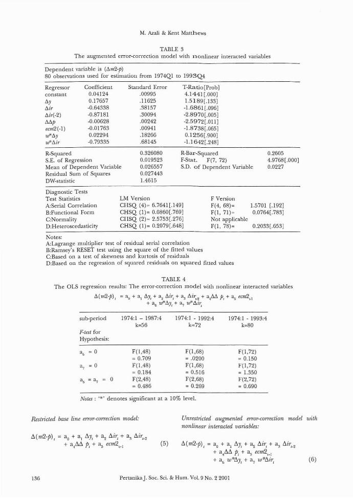
TABLE 3The augmented error-correction model with nonlinear interacted variables

Dependent variable is (6m2-p)80 obselVations used for estimation from 1974QI to 1993Q4

Regressorconstant6y6ir6,,,-2)Mpecm2(-I)w6yuJ'6ir

Coefficient0.041240.17657-0.64338-0.87181-0.00628-0.017630.02294-0.79335

Standard Error.00995.11625.38157.30094.00242.00941.18266.68145

T-Ratio[Prob)4.1441 [.000)1.5189[.133)-1.6861 [.096J-2.8970[.005J-2.5972[.0IlJ-1.8738[.065J0.1256[.900J-1.1642[.248)

R.SquaredS.E. of RegressionMean of Dependent VariableResidual Sum of SquaresOW-statistic

0.3260800.0195230.0265570.0274431.4615

R-Bar--SquaredF-Stat. F(7, 72)S.D. of Dependent Variable

0.26054.9768[.000)0.0227

Diagnostic TestsTest SlatisticsA:Serial CorrelationB:Functional FormC:Normality0:Heteroscedasticity

LM VersionCHSQ (4)~ 6.7641[.149)CHSQ (1)0 0.0860[.769JCHSQ (2)0 2.5753[.276]CHSQ (1)0 0.2079[.648)

F VersionF(4, 68)0F(l, 71)0Not applicableF(I, 78)0

1.5701 [.192J0.0764[.783J

0.2033[.653J

Notes:A:Lagrange lllulliplier test of residual serial correlationB:Ramsey's RESET test using the square of the fitted valuesC:Based on a test of skewness and kurtosis of residualsD:Based on the regression of squared residuals on squared fitted values

TABLE 4The OLS regression results: The error·correction model with nonlinear interacted variables

6(m2-p)j == ao + a\ 6YI + ~ 6ir, + (\3 6ir'.2 + ai~6. p, + a~ ecw2'.1+ a6 Ui"6y, + 3, TI1*~j~

sub-period

f"'-test forHypothesis:

" 00

" 00

" == a7 0

1974:1 - 1987:4k056

F(I,48): 0.709F(I,48)o 0.184F(2,48): 0.486

1974:1 - 1992:4k:72

F(I,68)o .0200F(I,68)00.516F(2,68)o 0.269

1974: I - 1993:4ko80

F(l,72): 0.150F(l,72)o 1.350F(2,72)o 0.690

NoUs: '*' denotes significant at a 10% level.

Restricted base litle error-correction model: Unrestricted augmented error-correction model withnonlinear interacted variables:

6(m2-p), = ao + a. 6y, + a2 6ir, + a:'l 6irJ-2+ a4M p, + a~ ecm2 L_ l

(5) 6(m2·p)1 = ao + a l 6.y, + ~ 6.ir, + a36irl-2+ a..6.6. PI + a~ ecm21_l

+ ali w*6Yt + a7 w*6irt (6)



The test results are reponed in Table 5 below.The tests in Table 5 indicate that all the nullhypotheses cannot be rejected, implying theoriginal restricted specification is not misspecified. However, whether the respecified'restricted' error-correction model (equation 5)can be regarded as a satisfactory short-run broadmoney demand function, depends on its abilityto provide adequate out-of-sample (ex post)forecasts. The results are reported in the nextsubsection.

earlier in Table 5, while results on equation (6)were reported in Table 4. Based on theseestimation results, it is clear that the originalmodel ('restricted' version) provided the bestoutcomes. Although they retained the desirablediagnostic residual properties, the estimates ofequation (6) indicate that the income variablewas insignificant. Therefore, the restrictedspecification (equation 5) was considered to bethe parsimonious model for broad moneydemand in this study.

TABLE 5Encompassing F-test - Restricted vs.

unrestricted models

Ex post Dynamic Forecast Results

A summary of the forecast statistics is detailed inTable 6. The results show that the root-meansquare prediction errors (rmse) of the originalrestricted model are quantitatively similar to theunrestricted models. In addition, all of theequations passed the predictive failure tests. AnFtest was also conducted to test the nullhypothesis that there is no difference in theaccuracy of these forecasts (see, Holden, Peeland Thompson 1990; pp. 33-37 for the details ofthe procedure). However, the latter test alsofailed to reject the null hypothesis. As analternative criterion to select the bestspecification, all equations were re-estimated andthen their properties were com pared. Theestimation results on equation (5) were reported

sample period1974ql-1991q41974ql-1992q41974ql-1993q4

Egn 5 vs. Egll 6F(2, 64) = 0.213[.808]F(2, 68) = 0.269[.764]F(2, 72) = 0.692[.504]

CONCLUSION

This study has shown that equation (5) is thepreferred error-correction specification for theshort~run broad money demand function, whileequation (4) for the long-run function. Theresults of encompassing tests and dynamic (expost) simulations confirm equation (5) as theparsimonious error-correction specification. Theinclusion of the nonlinear interacted variableswas unable to detect the underlying effects offinancial liberalization and innovations on thedemand for broad money in Malaysia.

The estimated short-run elasticities ofincome, cost of holding money, and inflation,are all reasonably estimated by the restrictedmodel as reponed in Table 2. Overall, theparsimonious model is rather simple, and itincludes basic explanatory variables in thecontemporary literature of money demandfunction.

Given the present results, the following twopolicy implications can be drawn from this study.First, the evidence supports the present strategytaken by the Malaysian monetary authority inmonitoring the growth of the broad monetaryaggregate as one of several strategies to curb

TABLE 6Summary statistics for ex post forecasts

Estimation period

Equation (5)1974:1 - 1992:4

Equation (6)1974:1 - 1992:4

Significance testamong the RMSE

Forecasting period

1993:1 - 1993:4

1993:1 - 1993:4

Hull Hypothesis, Ho:Equation (5) has asmaller RMSE thanequation (6)F(2.2) ::: 0.27

Predictive failure test

F(4, 70)= 1.597[.185J

F(4, 68)= 1.346[.262]

Conclusion:No difference in the

accuracy of theseforecasts

RMSE

0.025

0.025

PertanikaJ. Soc. Sci. & Hum. Vol. 9 No.2 2001 137


inflationary pressure. This study shows thatinflation has a significant negative impact on thedemand for real m2. For example, a 1% rise inthe price level could bring about a 0.58% declinein the demand for realm2, ceteris paribus. Hence,monetary policy has an important role incontrolling the price stability in Malaysia.

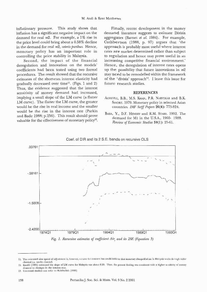
Second, the impact of the financialderegulation and innovation on the models'coefficients had been tested using two formalprocedures. The result showed that the recursiveestimates of the shon-run interest elasticity hadgradually decreased over time ll

. (Figs. 1 and 2)Thus, the evidence suggested that the interestsensitivity of money demand had increased,implying a small slope of the LM curve (a flatterLM curve). The flatter the LM cUn'e, the greaterwould be the rise in real income and the smallerwould be the rise in the interest rate (Parkinand Bade 1988; p.256). This result should provevaluable for the effectiveness of monetary policyl2.

Finally, recent development in the moneydemand literature suggests to estimate Divisiaaggregates (Barnet et ai. 1984). For example,Cuthbertson (1988, p. 97) argues that 'theapproach is probably most useful where interestrates are market determined rather than subjectto regulation and hence may prove useful in anincreasing competitive financial environment.'Hence, the deregulation of interest rates opensup the possibility that future innovations in m,2may need to be remodelled within the frameworkof the 'divisia' approach13

• I leave this issue forfuture research studies.

REFERENCES

ACHF-VU, RB., M.S. KHAi'>J, P.R. NARVEKA.R and B.K.SHORT. 1979. Monetary policy in selected Asiancountries. IMF Satff Papers 26(4): 775-824.

BABA, Y., D.F. HENDRY and R.M. STARR. 1992. Thedemand for MI in the U.S.A., 1960- 1988.Review of Economic Studies 59(1): 2.5-61.

Coel. 01 DIR and its 2 S.E. bands on recursive OLS

.33761 ,------------------------------,

/'

-.58161

,

)" ,

-1.5008 r-

-2.4200~=-:-"'~~~=~~~~~.......,~~.......~~~......,.=~~~~'_'_'<=~197401 197901 198401 198901 199304

Fig. 1. Recursive estimates of coefficient Llirl

and its 2SE (Equation 5)

I J. The eSlilllOlted slow sp",...d of adjustment is. howe"cr, a cause fur concern bm could indiCOlI<: tbat moo",l","y diseqUilibrium in ~1"J;,.rsi;l works through widerchanno:! i.e. credit challnd.

12. Kandil (1991) estimated the slope of LM cu",c for Mala}"ia was "bout 0.20. Thus. the pr"sent finding ""'" consistent with a higher &<:Ilsitivitl' of moneydemand to changes in the into;fcSI rate.

13 Interested readers can refer (0 Habibullah (1999)



CoeL 01 OIR and its 2 S.E. bands based on recursive OLS

·.0064007r-----------------------------,

, -

·.83014

·1.6539 . . ~ ,

.2.4776,~=-;-"-'~~_'_";=~~~=~~ft.1~~=~~~:;:;1;~~~~~~197301 197802 198303 198804 199304

Fig. 2. Recursive estimates of the coefficient of nir, (Equation 6)

BANK NECARA MA1.A\SIA. 1994. Money and Banking inMalaysia. Kuala Lumpur.

BANK NECARA MAlA\SIA. Quarterly Bulletin. Variousissues.

BARNET, W.A., E.K OFfENBACHER and P,A. SI'INDT.

1984, The new divisia monetary aggregates,Journal oj Political Economy 92(6): 11-48.

CACA.."l, P. and A. SCHWARTZ. 1975, Has the growth ofMmoney substitutes hindered monetary policy.Journal ojMoney, Credit, and Banking 7: 137-159.

CHOWDHURY, A.R. 1997. The financial structure andthe demand for money in Thailand. AppliedEconomics 29(3): 401-409.

CUTHBERTSON, K. 1988. The Supply and Demand JOTMone:>', New York: Basil Blackwell Inc,

DICKEY, D,A. and W, FULLER. 1979, Distribution ofthe estimatOrs for autoregressive time serieswith a unit root. Journal ojthe American StatisticalAssociation 74: 427-431.

DICKEY, D.A. and W. FULLER. 1981. The likelihoodratio statistics for autoregressive rime serieswith a unit root. Econometrica 49(4): 1057-1072.

ENGLE, R,F. and C.WJ. GRANGER. 1987, Cointegrationand error correction representation,estimation, and testing. Econometrica. 55(2): 251276.

FllIEDMAN, M, 1984, Lesson from the 1979·1982monetary policy experiment. The AmericanEconomic Review Papers and Proceedings 74: 339443.

FRY, MJ 1995, Money, Interest, and Ban!<ing inEconomic Development. Second Edition. London:The Johns Hopkins University Press.

GINSBURGII, V.A. 1973. A further note on thederivation of quarterly figures consistent 'vithannual da"'. Applied Statistics. 22: 368-374.

CURLEV,j.G. and E.S. SUAW. 1955. Financial aspectsof economic development. American Economic&view. 45(4): 515-538.

GURLEY, JG. and E,5. SHAW, 1960. 1\1oney in a The01)!of Finance, Washington D.C: BrookingsInstitution.

HABIBULLAlI, M,S. 1999. Divwa lvlonetary Aggregfltesand Economic Activities in Asian DevelopingEconomies. Aldershot: Ashgate.

HAQUE, A. and N. AL-MuTi\.IRL 1996, Financialderegulation, demand for narrow money andmonetary policy in Australia. Applied FinancialEconomics 6(4): 301-306,

PertanikaJ Soc, Sci. & Hum. Vol. 9 No.2 2001 139

M. Azali & Ken t Matthews

HENDRY, D.F. 1979. Predictive Failure andEconometric Modelling in Macroeconomics:The Transaction Demand for Money, Chapter9. In Economic Afodelling, ed. P. Ormerod. pp.217-242. London: Heinemann EducationBooks.

HEKDRY, D.F. and N.R. ERICSSON. 1991. Modellingthe demand for narrow money in the UnitedKingdom and the United States. EuropeanEconomic Review 35: 833-886.

HENDRY, D.F., A.R. PAGAN and J.D. SARGAN. 1984.Dynamic Specifications. In Handbook ofEconometrics, eds. Z. Griliches and M.D.Intriligator. Vo1.2. Amsterdam: North-Holland.

HESTER, D.D. 1981. Innovations and MonetaryControl, Brookings Papers in EconomicActivity, pp. 141-189.

HOLDEN, K, D.A. PEEL and J.L. THOMPSON. 1990.Economic Forecasting: An Introduction. New York:Cambridge University Press.

HOSSAIN, A. 1994. Financial deregulation, financialinnovation <Ind the stability of the Australianshort run narrow money demand function.Economics Noles 23(3): 410-437.

H\1.LEBERG, 5., R.F. ENGLE, C.WJ. GRA.NGER and B.S.

Yoo. 1990. Seasonal integration andcointegration. Journal of Econometrics 44: 21538.

INTERNATIONAL MONETARY FUND. InternationalFinancial Statistics, [monthly], Washington.Various issues.

ISMAIL, A.G. and P. SMITH. 1993. Monetary policyand commercial banks: an overview. JurnalEkonomi Malaysia 27: 29-55.

JOHANSEN, S. 1988. Statistical analysis of cointegrationvectors. Journal ofEconomic Dynamics and Control12: 231-254.

JOHANSEN, S. and K. JUSELIUS. 1990. Maximumlikelihood estimation and inference oncointegration - with application to the demandfor money. Oxford Bulletin of Economics andSlatistic 52(2): 169-210.

JOHANSEN, S. and K.JUSELIUS. 1992. Testing structuralhypotheses in a multivariate cointegrationanalysis of the PPP and the VIP for VKJournalof Econometrics 53: 211-244.

KANOlL, M. 1991. Structural differences betweendeveloping and developed countries: someevidence and implications. Economic Notes 20(2):254-278.

MOHAMED, A. 1996. Velocity and the variability ofanticipated and unanticipated money growthin Malaysia. Applied Economics Letters 3: 697-700.

MOHAMED, A. 1998. The monetary policytransmission mechanism: the Malaysianexperience during the pre-liberalization andpost-liberalization periods. Unpublished Ph.D.Thesis, University of Wales Cardiff, the UK.

MIZON, G.E. and J.F. RICHARD. 1986. Theencompassing principle and its application totesting non·nested hypotheses. Econometrica 54:657-678.

PARKIN, M. and R. BADE. 1988. Modern Macroeconomics.Hertfordshire: Simon and Schuster InternationalGroup.

PESARAN, M.H. and B. PESARAN. 1996. Working withMicrofit 4.0: Interactive Econometric Analysis,Oxford University Press.

PHlLLIPS, P.C.B. and P. PERRON. 1988. Testing for aunit root in time series regression. Biometrika75(2): 335-346.

TARIQ, S.M. and KG.P. MATTHEWS. 1996. Demandfor simple-sum and divisia monetary aggregatesfor Pakistan. Cardiff Business School WorkingPaper, University of Wales Cardiff, the UK.

TSENG, W. and R. CORKER. 1991. Financialliberalization, money demand and monetarypolicy in Asian countries, internationalmonetary fund. Occasional Paper No. 84,Washington D,C.

Received: 16 August 2001

140 PerL.1.nikaj. Soc. Sci. & Hum. Vol. 9 No.2 2001


DATA APPENDIX

Data used in the paper come from various issuesof the International Financial Statsistics publishedby the International Monetary Fund and theQuarterly Bulletin Bank egara Malaysia. Thequarterly data of the Industrial Production Index(/PI, 1990=100) were utilised to interpolate thequarterly GDPdata (y) using the Vangrevelinghe's

method (see Ginsburgh 1973)). Observationsspanning 1972:ql to 1993:q4. The variableswhich have been used in the paper are as follows:CD?· Gross Domestic Product; m2 - broad moneysupply; p- consumer price index (CPI, 1990=100);dr3 - 3-month deposit rate; and tbl3 - 3-monthTreasury bill rate.

PenanikaJ. Soc. Sci. & Hum. Vol. 9 No.2 2001 141

broad money demand and financial liberalization in...

Documents