tabu search for graph partitioning

Annals of Operations Research 63(1996)209-232 209

Tabu search for graph partitioning

Erik Rolland

The A. Gary Anderson Graduate School of Management, University of California, Riverside, CA 92521, USA

Hasan Pirkul

Academic Faculty of Accounting & MIS, The Ohio State University, Columbus, OH 43210, USA

Fred Glover

Graduate School of Business and Administration, University of Colorado at Boulder, Boulder, CO 80309, USA

In this paper, we develop a tabu search procedure for solving the uniform graph partitioning problem. Tabu search, an abstract heuristic search method, has been shown to have promise in solving several NP-hard problems, such as job shop and flow shop scheduling, vehicle routing, quadratic assignment, and maximum satisfiability. We compare tabu search to other heuristic procedures for graph partitioning, and demonstrate that tabu search is superior to other solution approaches for the uniform graph partitioning problem both with respect to solution quality and computational requirements.

Keywords: Heuristic search, graph partitioning, tabu search.

1. Introduction

The uniform, weighted graph partitioning problem (GPP) can be stated as follows: Given a graph G = ( V , E ) , where tVt = m = 2 n , we are asked to find a partition of V into two node sets VI and V2 such that V = V1 + V2 and V1 f3 V2 = O, and L Vll = IV21 = n, which minimizes the sum of the cost of edges having end-points in different sets.

There are a number of applications for the graph partitioning problem. In electronic circuit design, for example, the GPP models the task of placing electronic components on circuit boards, where the goal is to cluster the components to minimize the cost of inter-component communication (see, e.g., Feo and Khellaf [5]). An equivalent problem exists in computer memory paging. Here, the goal is to locate highly interrelated programs (or subroutines) in the same physical memory location

© J.C. Baltzer AG, Science Publishers

210 E. Rolland et al., Tabu search for graph partitioning

(called a page), to minimize swapping to secondary memory (i.e., a hard disk), Other applications exist for placement and layout problems, as in floor planning, where the goal is to cluster modules (tasks, machines, offices) that are highly interconnected (Dai and Kuh [3]).

The graph partitioning problem has been proven to be NP-hard (Garey et al. [8]). Due to the presumed computational intractability of obtaining and verifying an optimal solution, a number of heuristic solution procedures have been proposed, seeking to obtain good (if not optimal) solutions within a reasonable time limit. Enumerative methods encounter difficulty, resulting in part from the explosion in the number of feasible solutions as the problem dimension increases. (A 100-node problem contains more than 1029 feasible solutions.) The sheer size of the problem space makes the GPP a challenging problem.

The best known heuristic for solving the GPP is the Kernighan-Lin (KL) procedure (Kernighan and Lin [ 17]). This heuristic operates by generating a succession of component steps that result in swapping groups of nodes between the two node sets, thus generalizing the type of approach that employs single pair swaps. The method continues to employ such generalized swaps until reaching a local optimum, where none of the proposed alternatives succeeds in producing an improved solution. A later extension to the KL algorithm (Fiduccia and Mattheyses [6]) improves on the computational requirements by using largely single moves of nodes (instead of swaps) as well as smarter cost updates. The strength of the KL algorithm lies in the ability to locate good feasible solutions in a relatively small amount of time. It has been widely thought that this algorithm indeed guarantees very good solutions. However, the results of our research indicate there is significant room for improvement.

Recently, Johnson et al. [16] have reported on a simulated annealing (SA) procedure, and compared it to KL and local search. They concluded that for sparse problem instances, the SA procedure was inferior to KL when equalized for running time. Like tabu search, simulated annealing constitutes an abstract heuristic search procedure. These types of algorithms utilize general (or abstract) problem knowledge. Here, we outline a new procedure based on tabu search for solving the graph partitioning problem.

Tabu search (TS) is a meta-level heuristic for solving optimization problems. Any procedure which relies on transformations of problem states can be guided by TS, provided we have a measure to evaluate the attractiveness of alternative transformations. By iteratively performing transformations on the problem state, we seek to locate good feasible solutions. A comprehensive survey of tabu search can be found in Glover and Laguna [12].

Several implementations of TS for problems that share some of the features of the GPP have been reported. Glover et al. [14] provided an application to affinity- based clustering problems for architectural design and space planning. The TS approach incorporated constructive, destructive, and transfer moves (between different clusters), and accommodated problems with bounds on cluster sizes and on numbers of clusters.

E. Rolland et al., Tabu search for graph partitioning 211

Implemented in a system adopted by national space planning firms, the method produced solutions to problems whose integer programming formulation contained more than 60,000 integer variables, and resulted in "affinity bubble diagrams" superior to those created by trained architects.

Laguna et al. [20] developed a TS procedure for solving single-machine scheduling problems, which consist of minimizing the sum of setup costs and linear delay penalties when n jobs are to be scheduled for sequential processing on one machine. State space transformations were obtained using two strategies: either swapping pairs of jobs, or performing insertions by placing a selected job between two others. The quality of the TS solutions was found to be much better than those obtained using other heuristic procedures.

Taillard [27] and Chakrapani and Skorin-Kapov [2] have proposed parallel TS procedures for solving the quadratic assignment problem, where the goal is to find an assignment of n objects to n locations which minimizes the cumulative product of weighted flows between every two objects. The solution transformations are performed by pair-wise swapping assignments. For a collection of standard test problems, both TS procedures found solutions that matched or were superior to the best solutions previously reported in the literature. Similar outcomes have been obtained for applying TS methods to classical vehicle routing problems by Gendreau et al. [9] and by Osman [23].

Klincewicz [19] developed a TS procedure for solving the p-hub location problem, which consists of connecting secondary nodes to one of p hub nodes, where the hub nodes are connected to provide the main inter-node communication links. The locations of the hub nodes are to be determined. A problem state transformation consists of replacing a hub node by another (currently non-hub) node. The TS procedure was again found to be highly effective, obtaining new best solutions for several known test problems. More recently, a TS procedure by Skorin-Kapov and Skorin- Kapov [25] has obtained solutions dominating those previously found for a standard test bed of such problems. Other applications of TS are reported in Friden et ai. [7], Hertz et al. [15], de Werra et al. [4], and Glover et al. [13].

The remainder of this paper is structured as follows: an introduction to tabu search is given in section 2, together with a specialized TS procedure for solving GPPs. Computational results are presented in section 3. Section 4 discusses advanced issues related to the tabu search procedure, and section 5 summarizes our findings.

2. Tabu search for graph partitioning

Tabu search incorporates three general components: (i) short-term and long-term memory structures, (ii) tabu restrictions and aspiration criteria, and (iii) intensification and diversification strategies. Intensification strategies seek to integrate features or environments of good solutions as a basis for generating still better solutions. In the short-term, such strategies focus on aggressively searching for a best solution within


a strategically restricted region. Diversification strategies, which typically utilize a long- term memory function, redirect the search to unvisited regions of the solution space.

The principal mechanism for implementing the short-term memory function is a tabu list, or a collection of such lists, which record attributes of solutions (or moves) to forbid moves that lead to solutions that share attributes in common with solutions recently left behind (i.e., rendering such moves tabu). Aspiration criteria enable the tabu status of a move to be overridden, thus allowing the move to be performed, provided the move is rendered "good enough".

In our graph partitioning approach, we have undertaken to incorporate each of these elements in the simplest and most direct way. For the GPP setting, the tabu search procedure can begin either by strategically constructing an initial feasible starting solution or by generating such a solution randomly. We have elected a random starting procedure, which utilizes a uniform probability function ranging from 0 to 1 to determine the set membership for each node. The node is assigned to the set Vl if a randomly generated number drawn from this uniform probability distribution is less than 0.5, and to V 2 otherwise. If, at the end of this procedure the node sets are of unequal size, nodes are transferred from the larger set to the smaller using a greedy balancing procedure, until the sets are of equal size. The greedy balancing transfers a node from the larger to the smaller set, which results in the smallest possible cost increase (this is repeated until I Vii = ] V2I ). The procedure for obtaining a starting solution does not have a direct impact on our tabu search procedure, and can be accomplished using any random procedure.

We have also chosen the simplest type of move for changing the current solutions, which consists of selecting a single node v from either set, and transferring it to the other. The short-term memory function, embodied in a tabu list, is implemented as an array Tabu_Time(v) recording the most recent iteration at which the node v was moved. To prevent moving back to previously investigated solutions, we define a tabu time t as the time that must elapse before a node is permitted to be moved again, measured in number of iterations. If Current_Time denotes the current iteration, then a node v is tabu if T a b u T i m e ( v ) >_ Current_Time - t. The choice of t is critical to the performance of our implementation of the TS algorithm. For the GPP, we have empirically found 3~/n to be a good value for t. The rationale is that a tabu time larger than n can lead to problems in finding a non-tabu move, and the algorithm then wastes iterations without performing moves. A too short tabu time setting will lead to cycling (i.e., revisiting of previously tested problem states), and may prevent the algorithm from progressing into new (unvisited) problem states.

To prevent searching only a limited neighborhood of the current solution, we introduce an imbalance factor which allows the cardinality difference ("imbalance") in the two node sets to grow beyond 2 nodes (where the standard imbalance of 2 nodes stems from moving single nodes from one set to the other, starting with a feasible partition). When using the "standard" imbalance of 2 nodes, we effectively force every second iteration to result in a feasible solution. The idea behind using


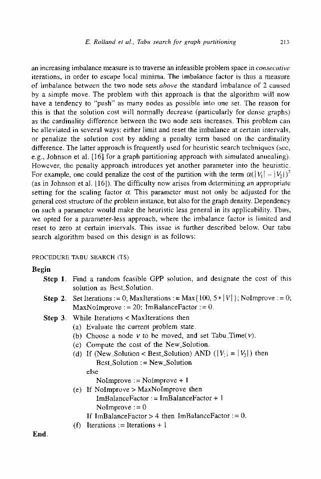
an increasing imbalance measure is to traverse an infeasible problem space in consecutive iterations, in order to escape local minima. The imbalance factor is thus a measure of imbalance between the two node sets above the standard imbalance of 2 caused by a simple move. The problem with this approach is that the algorithm will now have a tendency to "push" as many nodes as possible into one set. The reason for this is that the solution cost will normally decrease (particularly for dense graphs) as the cardinality difference between the two node sets increases. This problem can be alleviated in several ways: either limit and reset the imbalance at certain intervals, or penalize the solution cost by adding a penalty term based on the cardinality difference. The latter approach is frequently used for heuristic search techniques (see, e.g., Johnson et al. [16] for a graph partitioning approach with simulated annealing). However, the penalty approach introduces yet another parameter into the heuristic. For example, one could penalize the cost of the partition with the term a( [ Vl I - I VzD )2 (as in Johnson et al. [16]). The difficulty now arises from determining an appropriate setting for the scaling factor a. This parameter must not only be adjusted for the general cost structure of the problem instance, but also for the graph density. Dependency on such a parameter would make the heuristic less general in its applicability. Thus, we opted for a parameter-less approach, where the imbalance factor is limited and reset to zero at certain intervals. This issue is further described below. Our tabu search algorithm based on this design is as follows:

PROCEDURE TABU SEARCH (TS)

Begin Step 1.

Step 2.

Step 3.

End.

Find a random feasible GPP solution, and designate the cost of this solution as BestSolut ion.

Set Iterations : = 0; MaxIterations : = Max { 100, 5 * 1Vt }; NoImprove : = 0; MaxNoImprove : = 20; ImBalanceFactor : = 0.

While Iterations < MaxIterations then (a) Evaluate the current problem state. (b) Choose a node v to be moved, and set Tabu_Time(v). (c) Compute the cost of the NewSolut ion . (d) If (New_Solution < Best_Solution) AND (I Vii = ] V21) then

Bes tSolu t ion : = NewSolu t ion else

NoImprove := NoImprove + 1 (e) If NoImprove > MaxNoImprove then

ImBalanceFactor : = ImBalanceFactor + 1 NoImprove : = 0

If ImBalanceFactor > 4 then ImBalanceFactor : = 0. Iterations := Iterations + 1 (f)


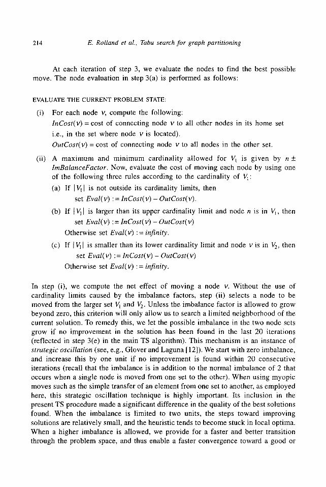
At each iteration of step 3, we evaluate the nodes to find the best possible move. The node evaluation in step 3(a) is performed as follows:

EVALUATE THE CURRENT PROBLEM STATE:

(i) For each node v, compute the following:

InCost(v) = cost of connecting node v to all other nodes in its home set

i.e., in the set where node v is located).

OutCost(v) = cost of connecting node v to all nodes in the other set.

(ii) A maximum and minimum cardinality allowed for V l is given by n + lmBalanceFactor. Now, evaluate the cost of moving each node by using one of the following three rules according to the cardinality of Vx:

(a) If I vll is not outside its cardinality limits, then

set Eval(v) := lnCost(v) - OutCost(v).

(b) If I Vll is larger than its upper cardinality limit and node n is in Vl, then

set Eval( v) := lnCost( v) - OutCost( v)

Otherwise set Eval(v) := infinity.

(c) If 1 Vii is smaller than its lower cardinality limit and node v is in V2, then

set Eval( v) := InCost( v) - OutCost( v)

Otherwise set Eval(v) := infinity.

In step (i), we compute the net effect of moving a node v. Without the use of cardinality limits caused by the imbalance factors, step (ii) selects a node to be moved from the larger set Vl and V2. Unless the imbalance factor is allowed to grow beyond zero, this criterion will only allow us to search a limited neighborhood of the current solution. To remedy this, we let the possible imbalance in the two node sets grow if no improvement in the solution has been found in the last 20 iterations (reflected in step 3(e) in the main TS algorithm). This mechanism is an instance of strategic oscillation (see, e.g., Glover and Laguna [12]). We start with zero imbalance, and increase this by one unit if no improvement is found within 20 consecutive iterations (recall that the imbalance is in addition to the normal imbalance of 2 that occurs when a single node is moved from one set to the other). When using myopic moves such as the simple transfer of an element from one set to another, as employed here, this strategic oscillation technique is highly important. Its inclusion in the present TS procedure made a significant difference in the quality of the best solutions found. When the imbalance is limited to two units, the steps toward improving solutions are relatively small, and the heuristic tends to become stuck in local optima. When a higher imbalance is allowed, we provide for a faster and better transition through the problem space, and thus enable a faster convergence toward a good or

E. Rolland et al., Tabu search f o r graph partitioning 215

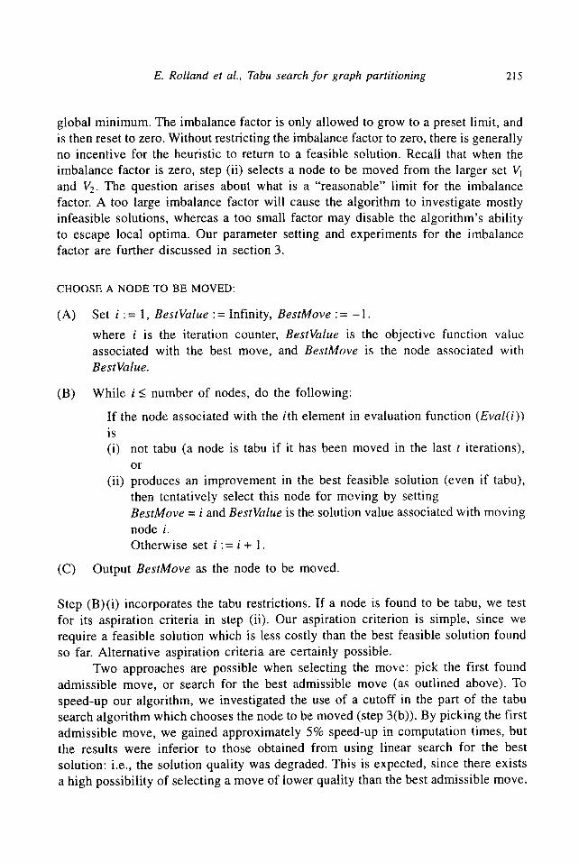
global minimum. The imbalance factor is only allowed to grow to a preset limit, and is then reset to zero. Without restricting the imbalance factor to zero, there is generally no incentive for the heuristic to return to a feasible solution. Recall that when the imbalance factor is zero, step (ii) selects a node to be moved from the larger set V l and V2. The question arises about what is a "reasonable" limit for the imbalance factor. A too large imbalance factor will cause the algorithm to investigate mostly infeasible solutions, whereas a too small factor may disable the algorithm's ability to escape local optima. Our parameter setting and experiments for the imbalance factor are further discussed in section 3.

CHOOSE A NODE TO BE MOVED:

(A) Set i : = 1, Bes tVa lue : = Infinity, B e s t M o v e : = - 1.

where i is the iteration counter, Bes tVa lue is the objective function value associated with the best move, and B e s t M o v e is the node associated with Bes tValue .

(B) While i < number of nodes, do the following:

If the node associated with the ith element in evaluation function ( E v a l ( i ) )

is (i) not tabu (a node is tabu if it has been moved in the last t iterations),

or (ii) produces an improvement in the best feasible solution (even if tabu),

then tentatively select this node for moving by setting B e s t M o v e = i and Bes tValue is the solution value associated with moving node i. Otherwise set i := i + 1.

(C) Output B e s t M o v e as the node to be moved.

Step (B)(i) incorporates the tabu restrictions. If a node is found to be tabu, we test for its aspiration criteria in step (ii). Our aspiration criterion is simple, since we require a feasible solution which is less costly than the best feasible solution found so far. Alternative aspiration criteria are certainly possible.

Two approaches are possible when selecting the move: pick the first found admissible move, or search for the best admissible move (as outlined above). To speed-up our algorithm, we investigated the use of a cutoff in the part of the tabu search algorithm which chooses the node to be moved (step 3(b)). By picking the first admissible move, we gained approximately 5% speed-up in computation times, but the results were inferior to those obtained from using linear search for the best solution: i.e., the solution quality was degraded. This is expected, since there exists a high possibility of selecting a move of lower quality than the best admissible move.


Our implementation as described to this point incorporates no long-term memory function, and thus no long-term diversification strategy. The "short-term diversification" created by strategic oscillation was anticipated in part to compensate for this, and thus our first experimentation focused on the short-term elements alone.

3. Computat ional results for short-term memory and strategic oscillation

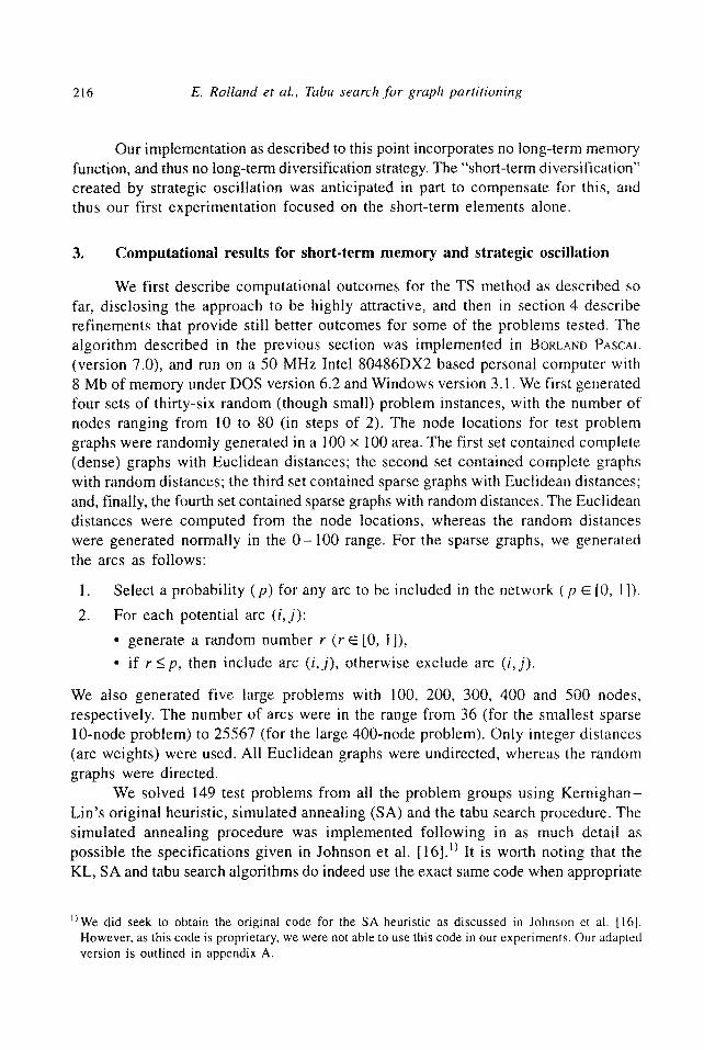
We first describe computational outcomes for the TS method as described so far, disclosing the approach to be highly attractive, and then in section 4 describe refinements that provide still better outcomes for some of the problems tested. The algorithm described in the previous section was implemented in BORLAND PASCAL (version 7.0), and run on a 50 MHz Intel 80486DX2 based personal computer with 8 Mb of memory under DOS version 6.2 and Windows version 3.1. We first generated four sets of thirty-six random (though small) problem instances, with the number of nodes ranging from 10 to 80 (in steps of 2). The node locations for test problem graphs were randomly generated in a 100 x 100 area. The first set contained complete (dense) graphs with Euclidean distances; the second set contained complete graphs with random distances; the third set contained sparse graphs with Euclidean distances; and, finally, the fourth set contained sparse graphs with random distances. The Euclidean distances were computed from the node locations, whereas the random distances were generated normally in the 0 - 1 0 0 range. For the sparse graphs, we generated the arcs as follows:

1. Select a probability (p) for any arc to be included in the network (p E [0, 1]).

2. For each potential arc (i , j) :

• generate a random number r (r ~ [0, 1 ]),

• if r<_p, then include arc (i , j) , otherwise exclude arc (i , j) .

We also generated five large problems with 100, 200, 300, 400 and 500 nodes, respectively. The number of arcs were in the range from 36 (for the smallest sparse 10-node problem) to 25567 (for the large 400-node problem). Only integer distances (arc weights) were used. All Euclidean graphs were undirected, whereas the random graphs were directed.

We solved 149 test problems from all the problem groups using Kemighan- Lin's original heuristic, simulated annealing (SA) and the tabu search procedure. The simulated annealing procedure was implemented following in as much detail as possible the specifications given in Johnson et al. [16]. 1) It is worth noting that the KL, SA and tabu search algorithms do indeed use the exact same code when appropriate

l~We did seek to obtain the original code for the SA heuristic as discussed in Johnson et al, [16]. However, as this code is proprietary, we were not able to use this code in our experiments. Our adapted version is outlined in appendix A.


(such as for solution evaluation). This ensures a fairer comparison of the algorithms. We also used the same data-structure (forward star) for all algorithms. This data- structure limits storage requirements to approximately IV] + ]El, as opposed to IV[ 2 if we had used a standard matrix structure. Without the efficient data-structure, the large problems are more difficult to solve on a personal computer (due to the limitation of 64K data-segments imposed by the DOS operating system).

The smaller problems (less than 20 nodes) are not challenging from a combinatorial standpoint, but are useful for demonstrating the essential difference in the kind of tuning considerations that may arise for small problems and larger ones. Note that in our experiments, we did not individually adjust the parameter settings (such as tabu time) when solving either large or small problems. Rather, we utilized parameter settings as functions of problem size, providing a more general tabu search algorithm.

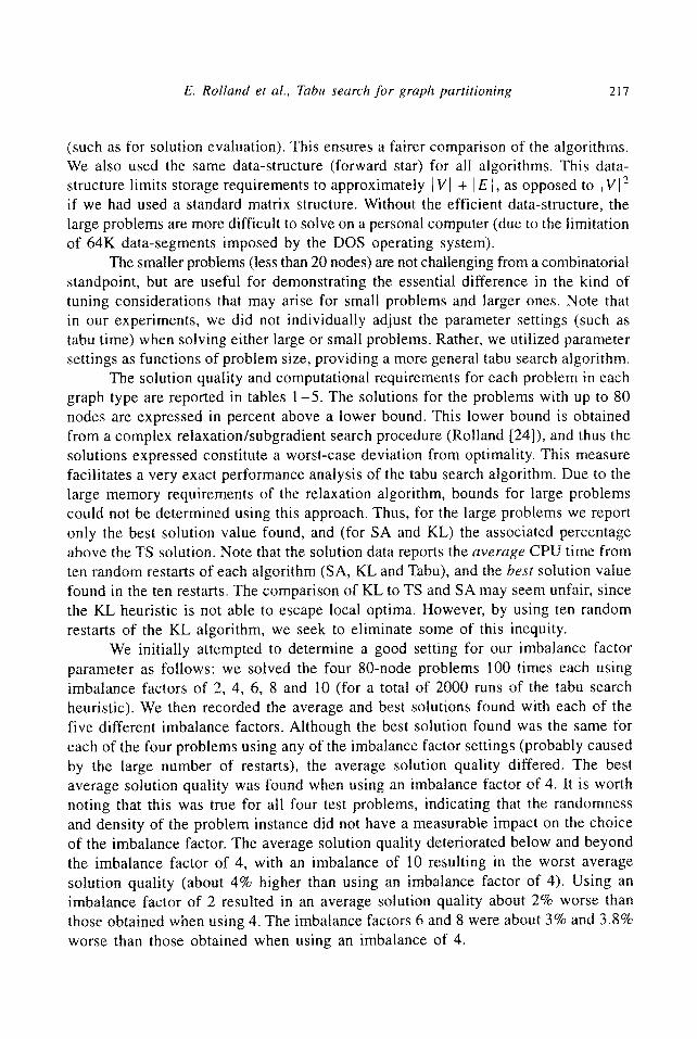
The solution quality and computational requirements for each problem in each graph type are reported in tables 1-5. The solutions for the problems with up to 80 nodes are expressed in percent above a lower bound. This lower bound is obtained from a complex relaxation/subgradient search procedure (Rolland [24]), and thus the solutions expressed constitute a worst-case deviation from optimality. This measure facilitates a very exact performance analysis of the tabu search algorithm. Due to the large memory requirements of the relaxation algorithm, bounds for large problems could not be determined using this approach. Thus, for the large problems we report only the best solution value found, and (for SA and KL) the associated percentage above the TS solution. Note that the solution data reports the average CPU time from ten random restarts of each algorithm (SA, KL and Tabu), and the best solution value found in the ten restarts. The comparison of KL to TS and SA may seem unfair, since the KL heuristic is not able to escape local optima. However, by using ten random restarts of the KL algorithm, we seek to eliminate some of this inequity.

We initially attempted to determine a good setting for our imbalance factor parameter as follows: we solved the four 80-node problems 100 times each using imbalance factors of 2, 4, 6, 8 and 10 (for a total of 2000 runs of the tabu search heuristic). We then recorded the average and best solutions found with each of the five different imbalance factors. Although the best solution found was the same for each of the four problems using any of the imbalance factor settings (probably caused by the large number of restarts), the average solution quality differed. The best average solution quality was found when using an imbalance factor of 4. It is worth noting that this was true for all four test problems, indicating that the randomness and density of the problem instance did not have a measurable impact on the choice of the imbalance factor. The average solution quality deteriorated below and beyond the imbalance factor of 4, with an imbalance of 10 resulting in the worst average solution quality (about 4% higher than using an imbalance factor of 4). Using an imbalance factor of 2 resulted in an average solution quality about 2% worse than those obtained when using 4. The imbalance factors 6 and 8 were about 3% and 3.8% worse than those obtained when using an imbalance of 4.


Table 1

AHS techniques applied to dense, Euclidean graphs.

Problem info Solution (% above bound)

Nodes Arcs SA KL Tabu

Average CPU times

SA CPU KL CPU Tabu CPU

10 90 4.24 5.44 4.24 2.88 0.05 0.12 12 132 12.24 12.97 8.76 4.87 0.05 0.20 14 182 1.90 9.53 1.90 8.19 0.24 0.25 16 240 1.39 4.82 1.39 14.94 0.26 0.33 18 306 1.39 9.12 1.39 24.17 1.10 0.38 20 380 0.01 9.18 0.01 39.88 0.89 0.46 22 462 0.94 8.68 0.00 50.10 1.26 0.66 24 552 0.63 8.72 0.15 66.93 1.75 0.86 26 650 0.23 9.73 0.03 78.52 1.59 0.97 28 756 0.69 6.98 0.00 274.10 3.15 1.15 30 870 1.05 8.21 0.05 153.36 6.76 1.57 32 992 1.65 9.46 1.37 291.44 5.2t 1.76 34 1122 2.24 6.85 2.17 216.05 I1.00 2.13 36 1260 2.27 8.38 0.12 275.21 5.44 2.56 38 1406 8.26 12.55 7~32 440.91 32.13 2.82 40 1560 2.21 9.43 0.10 585.75 8.15 3.42 42 1722 10.14 14.00 7.53 694.75 65.82 3.83 44 1892 8.16 10.85 6.84 996.04 35.20 4.36 46 2070 3.60 10.26 1.17 1021.08 7.01 5.05 48 2256 3.62 7.90 1.09 1279.54 24.56 5.86 50 2450 2.21 7.68 0.05 1093.04 28.10 6.50 52 2652 2.31 6.69 0.00 1903.95 68.50 7.34 54 2862 1.98 7.45 0.00 1536.31 40.01 8.06 56 3080 1.98 5.30 0.09 2031.90 91.35 9.13 58 3306 2.26 6.83 0.00 3327.03 70.12 10.80 60 3540 3.24 8.21 0.03 2262.12 60.25 11.23 62 3782 6.22 11.85 3.41 2235.07 45.00 11.86 64 4032 3.07 7.51 0.77 2528.64 75.21 13.32 66 4290 1.45 7.13 0.00 4492.18 144.20 15.03 68 4556 3.81 9.47 1.92 5038.19 64.80 15.82 70 4830 5.72 10.67 2.82 5160.29 145.10 18.04 72 5112 2.71 6.67 0. I1 5723.76 202.t0 19.55 74 5402 1.89 5.60 0.00 4462.4I 359.80 22.50 76 5700 10.61 12.98 8.45 6354.72 443.20 24.12 78 6006 9.69 14.40 7.68 7827.80 110.34 24.56 80 6320 7.27 10.38 4.85 5195.33 426.80 27.16

Average: 3.70 8.94 2.11 1880.31 71.85 7.88 Standard deviation: 3.24 2.45 2.86 2204.74 114.70 8.13 Minimum: 0.01 4.82 0.00 2.88 0.05 0.12 Maximum: 12.24 14.40 8.76 7827.80 443.20 27.16

SA: Simulated annealing. Tabu: Tabu search heuristic. KL: Kernighan-Lin's heuristic.


3.1. DENSE, EUCLIDEAN GRAPHS

As seen from table 1, the TS procedure required CPU times which increased roughly linearly with increasing problem size. A 10-node problem requires around 0.12 CPU seconds, whereas a 80-node problem required 27.16 seconds. Simulated annealing required on the average almost 5195 seconds to solve the 80-node problem, whereas Kernighan-Lin took about 427 seconds. The average number of iterations required by our TS procedure to find its best solution was 72. With some exceptions, this "convergence iteration" generally increased with increasing problem size. The convergence data is summarized in table 6. The average optimality gap for our TS approach was 2.11%, compared to 3.7% for SA and 8.94% for KL.

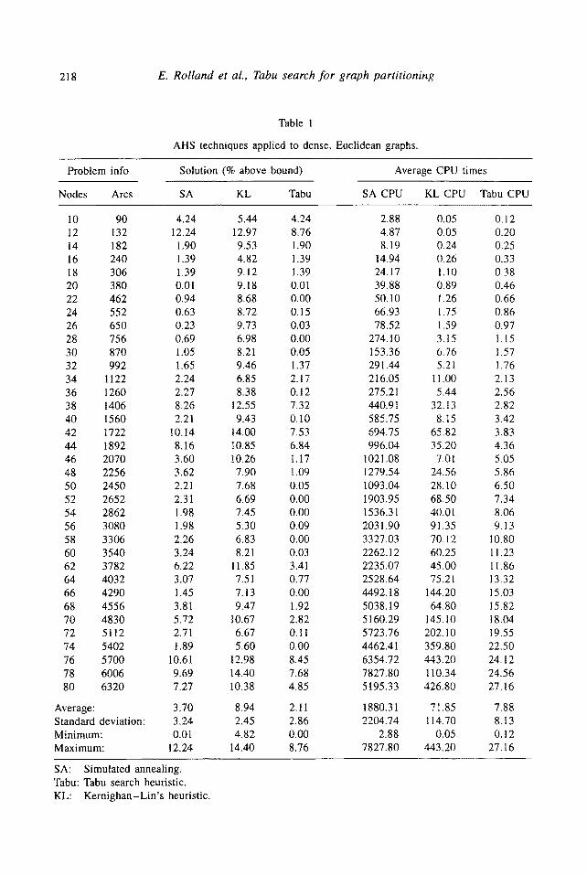
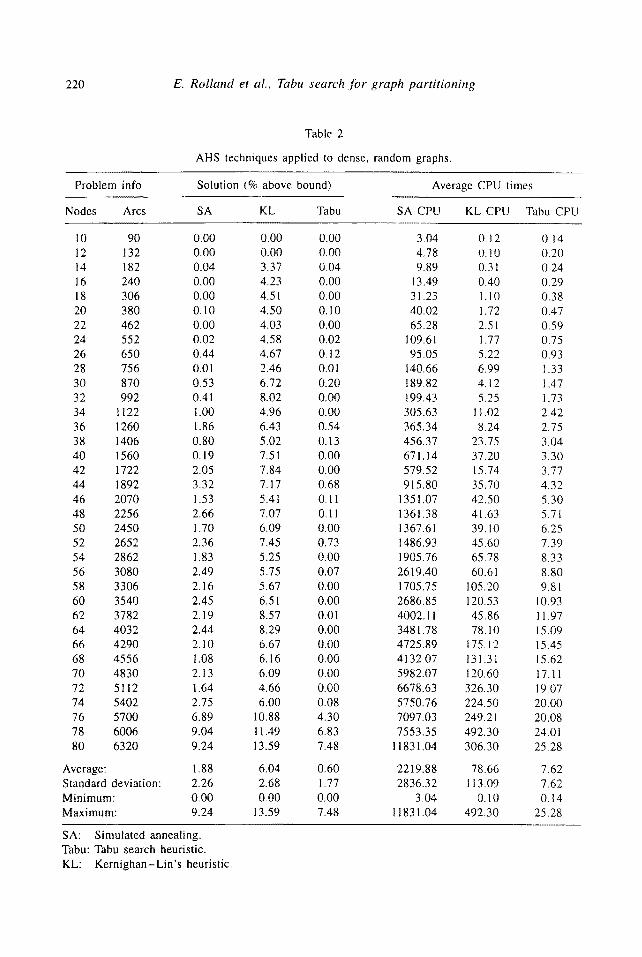
3.2. DENSE, RANDOM GRAPHS

For the dense, random graphs, our TS approach required between 0.14 and 25.3 CPU seconds to reach its cutoff point and terminate (table 2). SA required an average of 11831 seconds to solve the 80-node problem, and KL required 306 seconds. In general, the average time required by the SA method to obtain the best solution it was able to find was about 50% of its total running time, with a wide variance ranging from 4% all the way to 80% of its running time. The KL procedure, by its design (which elects termination when no improvement can be found), usually required 95% of its total running time before obtaining its best solution. The solution times for TS are linearly increasing with increasing problem size. The best solution was always found before iteration 97, and the average number of iterations for convergence was 48. No discrepancies between the running times for the Euclidean and the random dense graphs could be detected. However, all procedures improved the average bound with more than 1.5%. With some exceptions, the convergence iteration again generally increased with increasing problem size. The average gap for TS was a mere 0.6%, ranging from 0% to 7.5%. The average gap for SA was 1.88%, ranging from 0% to 9.24%, and the average gap for KL was 6.04%, ranging from 0% to 13.6%.

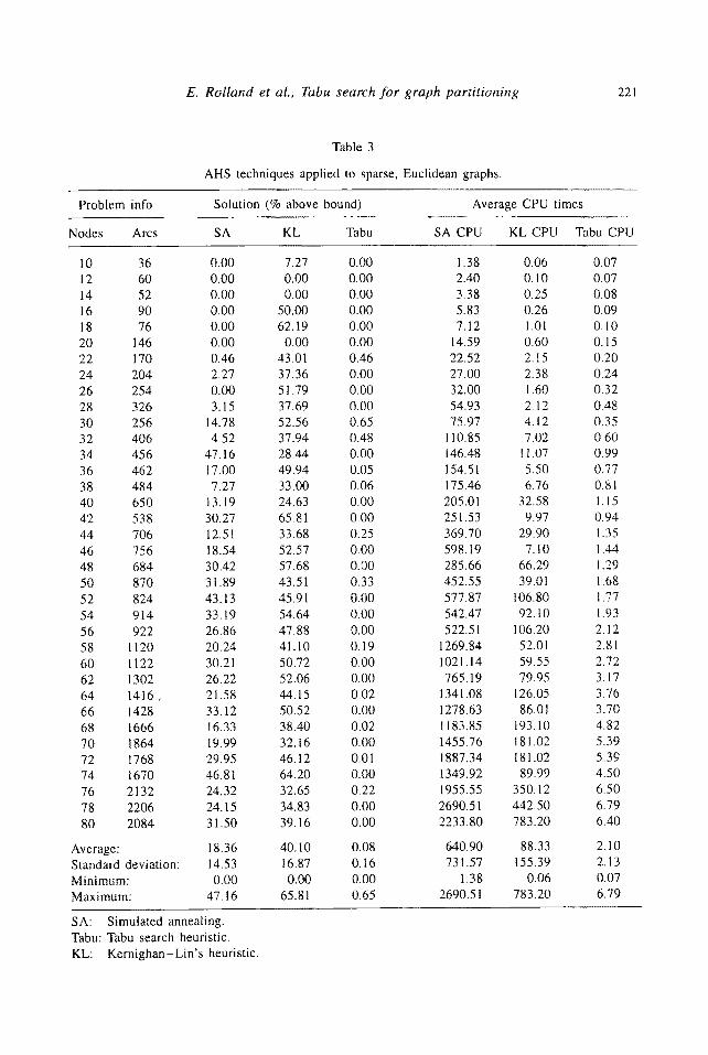
3.3. SPARSE, EUCLIDEAN GRAPHS

The sparse, Euclidean graphs required linearly increasing CPU times for TS (table 3), ranging from 0.07 seconds (10 nodes) to 6.8 seconds (78 nodes). The average number of iterations for convergence was 66. The gaps ranged from 0% to 0.65%, with an average of 0.08%. This graph type seemed difficult for both SA and KL, as indicated by average gaps of 18.4% and 40.1%, respectively. Thus, it seems that TS has a real edge for these problems.

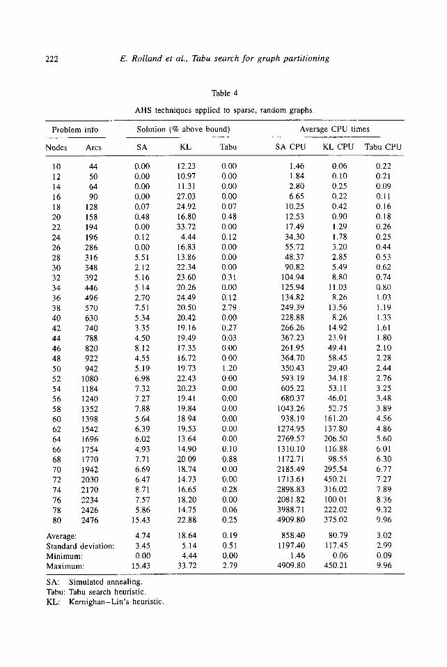
3.4. SPARSE, RANDOM GRAPHS

The CPU times for the sparse, random graphs confirmed the pattern of the CPU times for the other graph types: linearly increasing, between 0.09 and 9.96 CPU


Table 2

AHS techniques applied to dense, random graphs.



Average CPU times


10 90 0.00 0.00 0.00 3.04 0.12 0.14 12 132 0.00 0~00 0.00 4.78 0.10 0.20 14 182 0.04 3.37 0.04 9.89 0.31 0.24 16 240 0.00 4,23 0.00 13,49 0.40 0.29 18 306 0.00 4.51 0.00 31.23 1.10 0.38 20 380 0.10 4.50 0. I0 40.02 1.72 0.47 22 462 0.00 4.03 0.00 65.28 2.51 0,59 24 552 0.02 4.58 0.02 109.61 1.77 0.75 26 650 0.44 4.67 0.12 95.05 5.22 0.93 28 756 0.01 2.46 0.0l 140.66 6.99 1.33 30 870 0.53 6.72 0.20 189.82 4.12 1.47 32 992 0.41 8.02 0.00 199.43 5.25 1.73 34 1122 1.00 4.96 0.00 305.63 11.02 2.42 36 1260 1.86 6.43 0.54 365.34 8.24 2,75 38 1406 0.80 5.02 0.13 456.37 23.75 3.04 40 1560 0.19 7.51 0.00 671,14 37.20 3,30 42 1722 2.05 7.84 0.00 579.52 15.74 3.77 44 1892 3.32 7.17 0.68 915.80 35.70 4.32 46 2070 1.53 5.41 0.11 1351.07 42.50 5.30 48 2256 2.66 7.07 0.11 1361.38 41.63 5.71 50 2450 1.70 6.09 0.00 t 367.6 t 39.10 6.25 52 2652 2.36 7.45 0.73 t486.93 45.60 7.39 54 2862 1.83 5.25 0.00 1905.76 65.78 8.33 56 3080 2.49 5.75 0.07 2619.40 60.61 8.80 58 3306 2.16 5.67 0.00 1705.75 105.20 9.81 60 3540 2.45 6.51 0.00 2686.85 120.53 10.93 62 3782 2.19 8.57 0.01 4002.11 45.86 11.97 64 4032 2.44 8.29 0.00 3481.78 78.10 15.09 66 4290 2.10 6.67 0.00 4725.89 175.12 15.45 68 4556 1.08 6.I6 0.00 4132.07 131.31 15.62 70 4830 2.13 6.09 0.00 5982.07 120.60 17.11 72 5112 1.64 4.66 0.00 6678.63 326.30 19.07 74 5402 2.75 6.00 0.08 5750.76 224.50 20.00 76 5700 6.89 10.88 4.30 7097.03 249.21 20,08 78 6006 9.04 11,49 6.83 7553.35 492.30 24.01 80 6320 9.24 13.59 7.48 11831.04 306.30 25,28

Average: 1.88 6.04 0.60 2219.88 78.66 7.62 Standard deviation: 2.26 2.68 1.77 2836.32 113.09 7.62 Minimum: 0.00 0.00 0.00 3.04 O. 10 O. 14 Maximum: 9.24 13.59 7.48 11831.04 492.30 25.28


E. Rolland et al,, Tabu search for graph partitioning 22t

Table 3

AHS techniques applied to sparse, Euclidean graphs.



Average CPU times


t 0 36 0.00 7.27 0.00 12 60 0.00 0.00 0.00 14 52 0.00 0.00 0.00 16 90 0.00 50.00 0.00 18 76 0.00 62.19 0.00 20 146 0.00 0.00 0.00 22 170 0.46 43.01 0.46 24 204 2.27 37.36 0.00 26 254 0.00 51.79 0.00 28 326 3.15 37,69 0.00 30 256 14.78 52.56 0.65 32 406 4.52 37.94 0.48 34 456 47.16 28.44 0.00 36 462 17.00 49.94 0.05 38 484 7.27 33.00 0.06 40 650 13.19 24.63 0.00 42 538 30.27 65,81 0.00 44 706 12.51 33.68 0.25 46 756 18.54 52.57 0.00 48 684 30.42 57.68 0.00 50 870 3 t .89 43.51 0.33 52 824 43.13 45.91 0.00 54 914 33.19 54,64 0.00 56 922 26.86 47.88 0.00 58 1120 20.24 41,10 0.19 60 1122 30.21 50.72 0.00 62 1302 26.22 52.06 0.00 64 1416 ~ 21.58 44.15 0.02 66 1428 33.12 50.52 0.00 68 t666 16.33 38.40 0.02 70 1864 19.99 32. t6 0.00 72 1768 29.95 46.12 0.01 74 1670 46.81 64.20 0.00 76 2132 24.32 32.65 0.22 78 2206 24.15 34.83 0.00 80 2084 31.50 39.16 0.00

Average: 18.36 40.10 0.08 Standard deviation: 14.53 16.87 0.t6 Minimum: 0.00 0.00 0.00 Maximum: 47.16 65.81 0.65

1.38 0.06 0.07 2.40 0.10 0.07 3,38 0.25 0.08 5.83 0.26 0.09 7,12 1.01 0,10

14.59 0.60 0.15 22.52 2.15 0.20 27.00 2.38 0.24 32.00 1.60 0.32 54,93 2,12 0.48 75.97 4.12 0.35

110.85 7.02 0.60 t46.48 11.07 0.99 154.51 5.50 0.77 175,46 6.76 0.8 I 205.01 32.58 1.15 251.53 9.97 0.94 369.70 29.90 1.35 598.19 7.10 1.44 285.66 66,29 1,29 452.55 39.01 1.68 577,87 106.80 1.77 542.47 92.10 1.93 522.51 106.20 2.12

1269.84 52.01 2.81 1021.14 59.55 2.72 765.19 79.95 3.17

1341.08 126.05 3.76 1278.63 86.01 3.70 1183.85 193.10 4.82 1455.76 181.02 5.39 1887.34 t 81.02 5.39 1349.92 89.99 4.50 1955.55 350.12 6.50 2690.51 442.50 6.79 2233.80 783.20 6.40

640.90 88.33 2.10 731.57 155.39 2.13

1,38 0.06 0.07 2690.51 783.20 6.79



Table 4

AHS techniques applied to sparse, random graphs.



Average CPU times


10 44 0.00 12.23 0.00 12 50 0.00 10,97 0.00 14 64 0.00 11.31 0.00 16 90 0.00 27.03 0.00 18 128 0.07 24.92 0,07 20 158 0.48 16.80 0,48 22 194 0.00 33.72 0,00 24 196 0.12 4.44 0.12 26 286 0.00 16.83 0.00 28 316 5,51 13.86 0.00 30 348 2.12 22.34 0,00 32 392 5,16 23.60 0.31 34 446 5.14 20.26 0.00 36 496 2.70 24.49 0.12 38 570 7.51 20.50 2.79 40 630 5.34 20.42 0.00 42 740 3.35 19.16 0.27 44 788 4.50 19.49 0.03 46 820 8.12 17.35 0.00 48 922 4.55 16,72 0.00 50 942 5.19 19,73 1.20 52 1080 6.98 22.43 0.00 54 1184 7.32 20.23 0.00 56 1240 7.27 19.41 0.00 58 1352 7.88 19.84 0.00 60 1398 5,64 18.94 0.00 62 1542 6.39 19.53 0.00 64 1696 6,02 13.64 0.00 66 1754 4.93 14.90 0.10 68 1770 7,71 20.09 0.88 70 1942 6.69 18.74 0.00 72 2030 6.47 14.73 0.00 74 2170 8.71 16.65 0.28 76 2234 7.57 18.20 0.00 78 2426 5.86 14.75 0~06 80 2476 15.43 22.88 0.25

Average: 4.74 18.64 0.19 Standard deviation: 3,45 5.14 0.51 Minimum: 0.00 4.44 0.00 Maximum: 15.43 33.72 2,79

1.46 0,06 0.22 1.84 0,10 0.21 2.80 0,25 0.09 6.65 0,22 0.11

10.25 0.42 0.16 12.53 0.90 0.18 17.49 1.29 0.26 34.30 1.78 0.25 55.72 3.20 0.44 48.37 2.85 0.53 90.82 5,49 0.62

104.94 8,80 0.74 125.94 11.03 0.80 134.82 8.26 1.03 249.39 13.56 1.19 228.88 8.26 1.33 266.26 14.92 1.61 367.23 23.91 1.80 261.95 49.41 2.10 364.70 58,45 2.28 350.43 29.40 2.44 593.19 34,18 2.76 605.22 53.11 3.25 680.37 46.01 3.48

1043.26 52.75 3.89 938.19 161,20 4.56

1274.95 137.80 4.86 2769.57 206.50 5.60 1310,10 116.88 6.01 1172,71 98.55 6.30 2185.49 295.54 6.77 1713.61 450.21 7.27 2898.83 316.02 7.89 208I .82 I00.01 8.36 3988.71 222.02 9.32 4909.80 375.02 9.96

858.40 80.79 3.02 1197.40 117,45 2.99

1.46 0.06 0.09 4909.80 450,21 9.96

SA: Simulated annealing. Tabu: Tabu search heuristic, KL: Kernighan-Lin's heuristic.

E, Rolland et al., Tabu search for graph partitioning 223

seconds (table 4). The average number of iterations for convergence was 34. The average gap was 0.19%, ranging from 0% to 2.8%. Again, SA and KL had high average gaps of 4.74% and 18.64%, respectively. However, the gaps are about half of the average gaps for the sparse, Euclidean graphs for KL, and less than a fourth for SA. Tabu search required less computational time for the sparse graphs as opposed to the dense graphs. This is solely a function of the data-structure - for cost computations, we only need to investigate existing arcs.

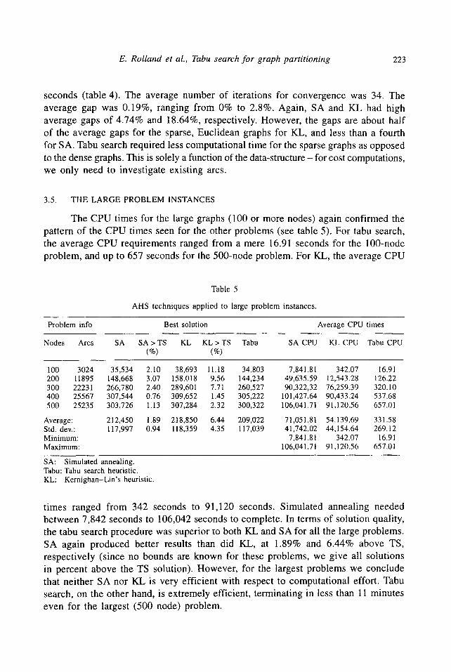
3.5. THE LARGE PROBLEM INSTANCES

The CPU times for the large graphs (100 or more nodes) again confirmed the pattern of the CPU times seen for the other problems (see table 5). For tabu search, the average CPU requirements ranged from a mere 16.91 seconds for the 100-node problem, and up to 657 seconds for the 500-node problem. For KL, the average CPU

Table 5

AHS techniques applied to large problem instances.

Problem info Best solution Average CPU times

Nodes Arcs SA SA > TS KL KL > TS Tabu SA CPU KL CPU Tabu CPU (%) (%)

100 3024 35,534 2.10 38 ,693 11 .18 3 4 , 8 0 3 7 , 8 4 1 . 8 1 342.07 16.91 200 1 1 8 9 5 148,668 3.07 158.018 9.56 1 4 4 , 2 3 4 49,635.59 12,543.28 126.22 300 2 2 2 3 1 266,780 2.40 289,601 7.71 260,527 90,322,32 76,259.39 320.10 400 25567 307,544 0.76 309,652 1.45 305 ,222 101,427.64 90,433.24 537.68 500 25235 303,726 1.13 307,284 2.32 300,322 106,041.71 91,120.56 657.01

Average: 212,450 1.89 2t8,850 6.44 2 0 9 , 0 2 2 71,051.81 54.t39.69 331.58 Std. dev.: 117,997 0.94 118,359 4.35 117 ,039 41,742,02 44,154.64 269.12 Minimum: 7,841.81 342.07 16.91 Maximum: 106,041.71 91,120.56 657.01


times ranged from 342 seconds to 91,120 seconds. Simulated annealing needed between 7,842 seconds to 106,042 seconds to complete. In terms of solution quality, the tabu search procedure was superior to both KL and SA for all the large problems. SA again produced better results than did KL, at 1.89% and 6.44% above TS, respectively (since no bounds are known for these problems, we give all solutions in percent above the TS solution). However, for the largest problems we conclude that neither SA nor KL is very efficient with respect to computational effort. Tabu search, on the other hand, is extremely efficient, terminating in less than 11 minutes even for the largest (500 node) problem.


4. Advanced issues and future directions

An evident intensification approach (that also has some elements of diversification) is to save the f~ best solutions in an array and use them as new starting solutions in the event no improvement has occurred in the last ~5 iterations. Used without refinement, this option is not likely to be highly effective when coupled with our approach, for evident reasons. Since the simple tabu search procedure described above is "serially myopic", the regions in the vicinity of previously found solutions have been fairly thoroughly investigated, given the state of the short-term memory. If solutions found earlier did not give good results, retrieving them at a later point will also do little good, unless the tabu list or the tabu time is changed. Thus, we can expect that restarting the algorithm from a previous good solution, without changing the tabu list/time, is unlikely to be especially productive for the TS procedure. However, if one alters the tabu list/time, this strategy could be worth investigating. For example, a recent application of Voss [28] for the quadratic assignment problems develops an effective variant of this strategy. In addition, the modification of resuming the search from good unselected neighbors of previous solutions, as suggested in Glover [11] (which allows tabu memory for these solutions to be retained), has produced new best solutions for job shop scheduling problems in the TS approach of Nowicki and Smutnicki [22].

4.1. RELATIVE POTENTIAL MERIT OF INTENSIFICATION AND DIVERSIFICATION

Three experiments with f2 = 1 and ~5={ 10, 20, 40}, respectively, were performed on all of the 144 small problem instances. The overall best solution was saved and used as a starting point if ~5 iterations expired without improvements in the best solution. The tabu time was kept unchanged, but the tabu list was cleared (i.e., "forgotten"). This strategy facilitates a local search in the neighborhood of previously found high-quality solutions. The experiments using ~5 = 10 and 6= 40 showed very few improvements in the best solutions found. Using ~5 = 10 restarted the algorithm too often, not giving it ample time to escape local optima, while using ~5 = 20 produced slight improvements in solution quality for about 10% of the test problems. Although the best improvement was almost 5%, the average improvement was negative: in other words, the overall solution quality was degraded by this approach (given the limit set on the number of iterations permitted to the search). This suggests three things: first, that the tabu time is appropriate; second that the strategic oscillation components allow enough latitude to locate local optima, as well as to escape these local optima; and third that gains in the present setting are more likely to result from a diversification strategy than an intensification strategy.

A naive type of diversification strategy is to restart the TS algorithm at different random starting solutions. One deficiency of this approach is that it automatically degrades the computational efficiency of TS. This approach was reported above in


section 3. For the problems that had poor gaps, the quality of the TS solution sometimes improved substantially (up to 3.5%). During our experiments, we found that the quality of the starting solution was not important, since the TS procedure easily escaped from both good and poor starting solutions. This confirmed the robustness of the short-term component of the procedure, and supported the supposition that further gains may be expected by consideration of more advanced diversification strategies.

4.2. FREQUENCY BASED MEMORY

The type of memory used in the standard short-term tabu list may be called recency based memory. Another integral type of memory in TS, typically suited to longer-term considerations, is frequency based memory.

One simple frequency based memory function for the GPP setting can be constructed by recording the number of times a node has been moved from one set to the other (i.e., from V 1 to V2). We chose to exploit this memory as follows: When the algorithm exhausts its initial productive surge (which occurs when the imbalance is allowed to increase beyond two for the first time), we attach a penalty to the cost of moving a node, consisting of a simple weighted function of the frequency count. Let Freq(i) denote the frequency based memory function, which records the number of times a node i has been moved from Vl to V2. The penalty function was then given the form P(i) = cFreq(i), where c is a constant. The purpose of this function is to provide a diversification into areas of the problem state that have not been investigated, but it also inhibits long-term cycling between problem states. Using a penalty weight of 10 (c = 10), we found that this frequency based memory function improved the performance of the tabu search algorithm. The average improvement in solution quality, when tested on the 144 smaller problems, was small (less than 1%) over the tabu search algorithm with no frequency based memory (but using random restarts - as reported in section 3). However, as compared to a single-start tabu search algorithm, we saw an average of almost 3% improvement in solution quality by using the penalty scheme (in one complete test of all our 144 problem instances with less than 100 nodes). Also, we found this penalty scheme eliminated the need for strategic oscillation, whose contributions to the solution process appeared to become superfluous when the frequency based memory was employed. We consider this a good indicator that strategic oscillation and longer-term memory (such as a penalty function) both help to accomplish effective diversification. However, for the graph partitioning problem we found no clear evidence that these techniques must be used together.

4.3. ASPIRATION CRITERIA

Several possibilities exist for experimenting with aspiration criteria, of which the following two seem particularly relevant:


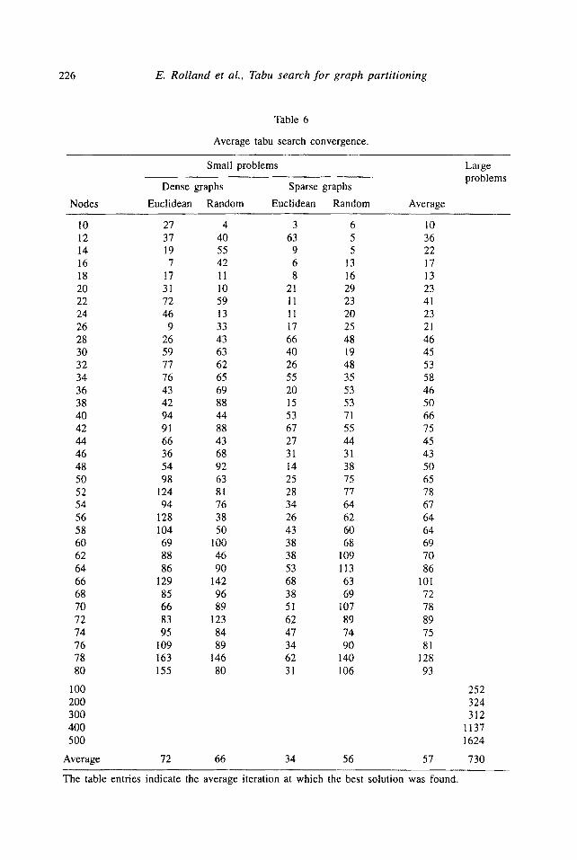
Table 6

Average tabu search convergence.

Nodes

Small problems

Dense graphs Sparse graphs

Euclidean Random Euclidean Random Average

Large problems

10 27 4 3 6 10 12 37 40 63 5 36 14 19 55 9 5 22 16 7 42 6 13 17 I8 17 11 8 16 13 20 31 10 21 29 23 22 72 59 11 23 41 24 46 13 11 20 23 26 9 33 17 25 21 28 26 43 66 48 46 30 59 63 40 19 45 32 77 62 26 48 53 34 76 65 55 35 58 36 43 69 20 53 46 38 42 88 15 53 50 40 94 44 53 71 66 42 91 88 67 55 75 44 66 43 27 44 45 46 36 68 31 31 43 48 54 92 14 38 50 50 98 63 25 75 65 52 124 81 28 77 78 54 94 76 34 64 67 56 128 38 26 62 64 58 104 50 43 60 64 60 69 100 38 68 69 62 88 46 38 109 70 64 86 90 53 113 86 66 129 142 68 63 101 68 85 96 38 69 72 70 66 89 51 107 78 72 83 123 62 89 89 74 95 84 47 74 75 76 109 89 34 90 81 78 163 146 62 140 128 80 155 80 31 106 93

100 200 300 400 500

Average 72 66 34 56 57

252 324 312

1137 1624

730

The table entries indicate the average iteration at which the best solution was found.


• Use different aspiration criteria for feasible and infeasible solutions.

• Use different aspiration criteria for the two-node sets: one restrictive, and one less restrictive.

The reasoning behind the separate aspiration criteria for feasible and infeasible solutions is quite clear: one does not want to restrict the possible creation of good feasible solutions (i.e., moving to another neighborhood). However, aspiration criteria which do not require feasibility should only be used when considering a possible move of a tabu node. Thus, if the tabu time is too tong one would require the aspiration criteria to be used more frequently. If the tabu time is of adequate length, the importance of this type of aspiration criteria is scaled down. More research is necessary in order to determine which aspiration criteria (other than the one used above) are "correct" in a graph partitioning setting. Thus we defer this issue to future research.

4.4. OTHER IMPROVEMENTS

The efficiency of tabu search can be improved in several ways. First, there exist opportunities in calibrating the number of iterations the TS procedure should be allowed to run. By studying the pattern of when the best solutions were found, we conclude that 5 * IV] iterations are sufficient for our large test problem, using our implementation. The procedure rarely found the best solution after these many iterations, even when allowing an upper limit of 100 * I vI iterations. A maximum limit lower than 100 is not appropriate, assuming some "margin of safety" is desired, since the TS procedure frequently needed up to 60 iterations to find the best solution for some of the smaller problems (< 100 nodes). In table 6, we report the TS convergence outcomes for our smaller test problems. These data do indeed support our setting for the maximum number of iterations needed.

Second, there are opportunities to incorporate additional local search mechanism into the TS procedure by applying simple exchange moves to preserve feasibility, thus allowing a descent method to be initiated from any feasible TS solution. This form of integrated local search can be seen, in fact, as an extension to the intensification strategy. Also a greedy type of balancing heuristic (similar to that of Johnson et al. [16]) can be applied to any infeasible solution. We found that the use of a balancing strategy resulted in excessive computing times, increasing the CPU time requirement by an average factor of 10 for our 144 small test problems. This increase in the running times led to no average improvements in the quality of the solutions. Applying local search in the form of descent moves initiated from all feasible TS solutions results in a slight increase in the running times, but also no further improvements in solution quality. This indicates that the short-term memory did not restrict the tabu search algorithm from fully investigating local optima.


5. Summary and conclusions

We have introduced a new technique for solving the graph partitioning problem based on tabu search. The use of strategic oscillation is shown to compensate for a lack of long-term memory, and effectively accomplishes diversification. The approach is superior to pure random restarting in that it incrementally improves on the current solution, without disregarding the information obtained from previous iterations. Thus, strategic oscillation provides a smoother transition through the solution space, where local optima are escaped by providing a proper choice of tabu restrictions (tabu time). A frequency based memory function was also examined, and found to vastly improve on the tabu search procedure that used only recency based memory. This memory function was also found effective even without the use of strategic oscillation, and allowed for large transitions through the problem space.

Computational times with our tabu search algorithm are predictable and independent of the underlying problem cost structure (with the exception of the number of arcs). Unlike simulated annealing and Kemighan-Lin 's heuristic, the CPU requirement for our approach is a direct increasing function of the problem size (and the maximum number of iterations). Also, the CPU requirement is for most problems only a fraction of that required by simulated annealing and Kernighan- Lin's heuristic. The CPU times required by TS for the 500-node problem is about 0.5% of the time required by SA. From our computational experience, we conclude that TS is better suited than both SA and KL for solving sparse GPP problems since the average gap of TS from an "idealized" bound is close to 0.1%, whereas SA and KL have average gaps of about 11% and 29%, respectively. TS produces better solutions than SA and KL for dense graphs as well, but the relative differences are smaller, with average gaps of 2.8%, 7.5% and 1.3%, respectively, for SA, KL and TS. The CPU memory requirements of tabu search are in general very modest, and we have demonstrated that even the large problems can be solved using inexpensive equipment (such as a personal computer).

There are several ways our approach can be refined. One is to incorporate dynamic tabu list management schemes. Another is to use more advanced types of aspiration criteria. A third is to incorporate learning considerations into long-term memory strategies. Discussions of these considerations, and applications in other settings where they have proved of value, are given in Glover and Laguna [12] and in Glover et al. [13].

In summary, we have seen that tabu search is very competitive, both with respect to solution quality and CPU time requirements. Tabu search outperforms by far simulated annealing and Kernighan-Lin's heuristic for solving the uniform graph partitioning problem, both with respect to computational time requirements and solution quality. In addition, we anticipate that deeper examination of strategic issues, such as those we have indicated in section 4, may lead to further improvements.


Acknowledgements

We wish to thank three anonymous referees for suggestions that helped improve the quality and presentation of this research. This research was supported in part under the Air Force Office of Scientific Research and Office of Naval Research Contract F49620-90-C-0033 at the University of Colorado.

Appendix

In this appendix, we outline the algorithms used for the simulated annealing and Kernighan-Lin heuristics. We state the pseudo-code for the algorithms, as well as all associated parameters.

A.1. THE SIMULATED ANNEALING HEURISTIC

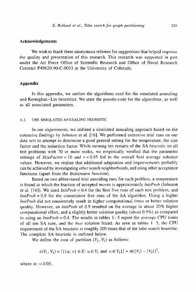
In our experiments, we utilized a simulated annealing approach based on the extensive findings by Johnson et al. [16]. We performed extensive trial runs on our data sets to attempt to determine a good general setting for the temperature, the size factor and the reduction factor. While running ten restarts of the SA heuristic on all test problems with 70 or more nodes, we empirically verified that the parameter settings of SizeFactor= 16 and r - -0 .95 led to the overall best average solution values. However, we realize that additional adaptation and improvements probably can be achieved by investigating other search neighborhoods, and using other acceptance functions (apart from the Boltzmann function).

Based on two abbreviated trial annealing runs for each problem, a temperature is found at which the fraction of accepted moves is approximately InitProb (Johnson et al. [16]). We used InitProb = 0.4 for the first five runs of each test problem, and lnitProb = 0.9 for the consecutive five runs of the SA algorithm. Using a higher InitProb did not consistently result in higher computational times or better solution quality. However, an lnitProb of 0.9 resulted on the average in about 20% higher computational effort, and a slightly better solution quality (about 0.5%) as compared to using an InitProb = 0.4. The results in tables 1 -5 report the average CPU times of all ten SA runs, and the best solution found. As seen in tables 1-5, the CPU requirement of the SA heuristic is roughly 200 times that of the tabu search heuristic. The complete SA heuristic is outlined below.

We define the cost of partition (V1, V2) as follows:

c(Vl, V2)= [{{u, v} ~ E : u ~ V 1 and v E V2}I + a ( lV l] - ]V2I) 2,

where a := 0.05.


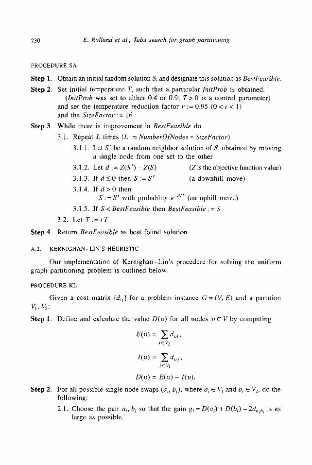
PROCEDURE SA

Step 1. Obtain an initial random solution S, and designate this solution as BestFeasible.

Step 2. Set initial temperature T, such that a particular lni tProb is obtained. ( lni tProb was set to either 0.4 or 0.9; T > 0 is a control parameter)

and set the temperature reduction factor r : = 0.95 (0 < r < 1) and the S i zeFac tor := 16

Step 3. While there is improvement in BestFeasible do

3.1. Repeat L times (L ' = NumberOfNodes * SizeFactor)

3.1.1. Let S ' be a random neighbor solution of S, obtained by moving a single node from one set to the other.

3.1.2. Let d := Z ( S ' ) - Z(S) (Z is the objective function value)

3.1.3. If d < 0 then S : = S ' (a downhill move)

3.1.4. I f d > 0 t h e n S := S' with probablity e -d/r (an uphill move)

3.1.5. If S < BestFeasible then BestFeasible := S

3.2. Let T : = r T

Return BestFeasible as best found solution. Step 4.

A.2. KERNIGHAN-LIN'S HEURISTIC

Our implementation of Kernighan-Lin 's procedure for solving the uniform graph partitioning problem is outlined below.

Step 1.

PROCEDURE KL

Given a cost matrix [d/j] for a problem instance G = (V, E) and a partition vl, v2:

Define and calculate the value D ( v ) for all nodes v E V by computing

e ( , . , ) =

iE V 2

l(v)= E d v j ,

D(u) = E ( v ) - l (v ) .

Step 2. For all possible single node swaps (ai , b i ) , where a i E V 1 and bi E V2, do the following:

2.1. Choose the pair ai, b i s o that the gain gi = O(ai) + D(bi) - 2d, ih i is as large as possible.


Step 3.

S t e p 4.

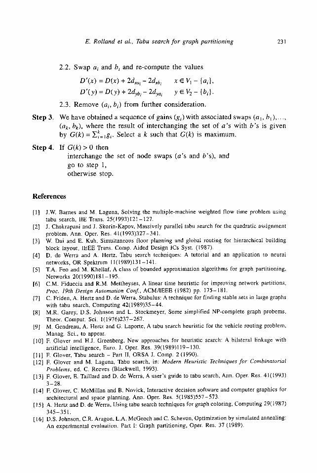
2.2. Swap a i and b i and re -compute the values

D'(x) = D(x) + 2dxai- 2dxbi x ~ V~ - {ai},

D ' ( y ) = D(y ) + 2dybi- 2dya, y ~ V2 - {bi}.

2.3. R e m o v e (a i, bi) f rom further considerat ion.

We have obta ined a sequence of gains (gi)wi th associated swaps (a l, b l) . . . . . (ak, bk), where the result o f interchanging the set o f a ' s with b ' s is g iven

by G ( k ) = ~ki=lg i. Select a k such that G(k) is max imum.

I f G(k) > 0 then in terchange the set o f node swaps ( a ' s and b ' s ) , and

go to step 1,

o therwise stop.

References

[1] J.W. Barnes and M. Laguna, Solving the multiple-machine weighted flow time problem using tabu search, IIE Trans. 25(1993)I21-127.

[2] J. Chakrapani and J. Skorin-Kapov, Massively parallel tabu search for the quadratic assignment problem, Ann. Oper. Res. 41(1993)327-341.

[3] W. Dai and E. Kuh, Simultaneous floor planning and global routing for hierarchical building block layout, IEEE Trans. Comp. Aided Design ICs Syst. (1987).

[4] D. de Werra and A. Hertz, Tabu search techniques: A tutorial and an application to neural networks, OR Spektrum 11(1989)131-141.

[5] T.A. Feo and M. Khellaf, A class of bounded approximation algorithms for graph partitioning, Networks 20(1990)181-195.

[6] CM. Fiduccia and R.M. Mettheyses, A linear time heuristic for improving network partitions, Proc. 19th Design Automation Conf., ACM/IEEE (1982) pp. 175-181.

[7] C. Friden, A. Hertz and D. de Werra, Stabulus: A technique for finding stable sets in large graphs with tabu search, Computing 42(1989)35-44.

[8] M.R. Garey, D.S. Johnson and L. Stockmeyer, Some simplified NP-complete graph probems, Theor. Comput. Sci. 1(1976)237-267.

[9] M. Gendreau, A. Hertz and G. Laporte, A tabu search heuristic for the vehicle routing problem, Manag. Sci., to appear.

[10] F. Glover and H.J. Greenberg, New approaches for heuristic search: A bilateral linkage with artificial intelligence, Euro. J. Oper. Res. 39(1989)119-130.

[11] E Glover, Tabu search - Part II, ORSA J. Comp. 2 (1990). [12] F. Glover and M. Laguna, Tabu search, in: Modern Heuristic Techniques for Combinatorial

Problems, ed. C. Reeves (Blackwell, 1993). [13] F. Glover, E. Taillard and D. de Werra, A user's guide to tabu search, Ann. Oper. Res. 41(1993)

3-28. [14] E Glover, C. McMillan and B. Novick, Interactive decision software and computer graphics for

architectural and space planning, Ann. Oper. Res. 5(1985)557-573. [15] A. Hertz and D. de Werra, Using tabu search techniques for graph coloring, Computing 29(1987)

345- 351. [16] D.S. Johnson, C.R. Aragon, L.A. McGeoch and C. Schevon, Optimization by simulated annealing:

An experimental evaluation. Part I: Graph partitioning, Oper. Res. 37 (1989).


[17] B.W. Kernighan and S. Lin, An efficient heuristic procedure for partitioning graphs, Bell Syst. Tech. J. 49(1970).

[18] S. Kirkpatrick, C.D. Gelatt and M.P. Vecchi, Optimization by simulated annealing. Science 220( 1983)671 - 680.

[I9] J.G. Klincewicz. Avoiding local optima in the p-hub location problem using tabu search and grasp, Ann. Oper. Res. 40(1992)121-132.

[20] M. Laguna, J,W. Barnes and E Glover, Tabu search methods for a single machine scheduling systems, J. Int. Manufact. 2(1991)63-74,

[21] M. Laguna and F. Glover, Integrating target analysis and tabu search for improved scheduling systems, Expert Syst. Appl. 6(1993)287-297.

[22] E. Nowicki and C. Smutnicki, A fast tabu search algorithm for the job shop problem. Technical Report, Technical University of Wroclaw, Poland (1993).

[23] I.H. Osman, Metastrategy simulated annealing and tabu search algorithms for the vehicle routing problem, Ann. Oper. Res. 41(1993)421-451.

[24] E. Rolland, Abstract heuristic search methods for graph partitioning, Ph.D. Dissertation, The Ohio State University, Colombus, OH (1991).

[25] D. Skorin-Kapov and J. Skorin-Kapov, On tabu search for the location of interacting hub facilities, Harriman School for Management and Policy, SUNY at Stony Brook (1992).

[26] J. Skorin-Kapov, Tabu search applied to the quadratic assignment problem, ORSA J. Comp. 2 (1990).

[27] E. Taillard, Robust tabu search for the quadratic assignment problem, Parallel Comp. 17(1991) 443 -455.

[28] S. Voss, An enhanced tabu search method for the quadratic assignment problem, Technical Report, Technische Hochschule Darmstadt (1993), to appear in Discr. Appl. Math.

tabu search for graph partitioning

Documents