grid-graph partitioning - computer sciences department - university
TRANSCRIPT

GRID-GRAPH PARTITIONING
By
William W. Donaldson
A dissertation submitted in partial fulfillment of the
requirements for the degree of
Doctor of Philosophy
(Computer Sciences)
at the
UNIVERSITY OF WISCONSIN – MADISON
2000

i
Abstract
Previous researchers showed that striping techniques produced very good (and, in some
cases, asymptotically optimal) partitions when applied to grid graphs. These striping
algorithms can be thought of as two-phase methods. The first phase consists of breaking
the original problem into smaller, but similar, problems (striping). The second phase
(stripe assignment) consists of the actual assignment of cells within the stripes. Results
from this reseach show how to improve both phases.
We improve the stripe-assignment phase of Christou, Meyer and Yackel so as to
guarantee locally optimal solutions for rectangular grid graphs. It is shown that under
certain assumptions, the assignment algorithm of Christou-Meyer will produce a locally
optimal solution. This algorithm is extended to handle a larger class of grid graphs. A
third algorithm is described that produces a locally optimal solution for the same class
of problems and also potentially reduces the chance of producing solutions with certain
undesirable characteristics.
In the striping phase, the methods of Yackel-Meyer, Christou-Meyer, and Martin dif-
fer in the stripe-height selection process. Yackel-Meyer and Christou-Meyer use genetic
algorithms for generating feasible solutions for a general class of grid graphs. Martin con-
siders rectangular domains and transforms the original problem into a knapsack problem
and considers a large set of stripe heights. Under the assumption that a stripe-assignment
approach satisfying certain generic conditions is given, we derive a dynamic-programming
method that generates the best possible set of stripe heights.

ii
Acknowledgements
I would like to thank my major professor, Robert R. Meyer, for giving me the opportunity
to work in a subject area that I enjoy and for helping me attain a life-long goal. I
would also like to thank professors Eric Bach (Reader), Steven Bauman, Deborah Joseph
(Reader), and Olvi Mangasarian for serving on my committee.
I would like to acknowledge Amir Roth and Victor Zandy for their help with imple-
mentation and performance-measurement issues.
I would like to thank several families outside the academic community. These persons
showed me a level of kindness that certainly was not expected. And although they will
remain anonymous, I will never forget what they did for me.
I would also like to acknowledge the use of hardware that was funded under NSF
grant CDA-9623632.

iii
Contents
Abstract i
Acknowledgements ii
1 Introduction 1
1.1 Problem Description . . . . . . . . . . . . . . . . . . . . . . . . . . . . . 1
1.2 Alternative Formulations of Graph Partitioning . . . . . . . . . . . . . . 2
1.2.1 Quadratic and Mixed Integer Programming Formulations . . . . . 2
1.2.2 Minimum Perimeter Formulation . . . . . . . . . . . . . . . . . . 4
1.3 Motivation and Background . . . . . . . . . . . . . . . . . . . . . . . . . 6
1.4 Contributions of this Dissertation . . . . . . . . . . . . . . . . . . . . . . 8
1.4.1 Local Optimality Assignments within Stripes . . . . . . . . . . . . 8
1.4.2 Stripe-Height Selection . . . . . . . . . . . . . . . . . . . . . . . . 9
1.5 Organization of this Dissertation . . . . . . . . . . . . . . . . . . . . . . 10
2 Background and Related Work 11
2.1 Introduction . . . . . . . . . . . . . . . . . . . . . . . . . . . . . . . . . . 11
2.2 Non-Striping Partitioning Algorithms . . . . . . . . . . . . . . . . . . . . 12
2.2.1 Kernighan-Lin . . . . . . . . . . . . . . . . . . . . . . . . . . . . . 12
2.2.2 Geometric Mesh Partition . . . . . . . . . . . . . . . . . . . . . . 13
2.2.3 Recursive Spectral Bisection . . . . . . . . . . . . . . . . . . . . . 14
2.2.4 METIS . . . . . . . . . . . . . . . . . . . . . . . . . . . . . . . . . 16
2.3 Stripe-Based algorithms . . . . . . . . . . . . . . . . . . . . . . . . . . . 17

iv
2.3.1 Stripe Assignments based on Genetic Algorithms . . . . . . . . . 19
2.3.2 Yackel-Meyer Algorithm . . . . . . . . . . . . . . . . . . . . . . . 20
2.3.3 Christou-Meyer Algorithm . . . . . . . . . . . . . . . . . . . . . . 20
2.3.4 Knapsack Algorithm . . . . . . . . . . . . . . . . . . . . . . . . . 23
2.3.5 The Shortest-Path/Dynamic-Programming Approach . . . . . . . 24
2.4 Improved Stripe Assignment . . . . . . . . . . . . . . . . . . . . . . . . . 25
2.5 Summary . . . . . . . . . . . . . . . . . . . . . . . . . . . . . . . . . . . 25
3 Improved Stripe Assignment 26
3.1 Introduction . . . . . . . . . . . . . . . . . . . . . . . . . . . . . . . . . . 26
3.2 Terms and Definitions . . . . . . . . . . . . . . . . . . . . . . . . . . . . 28
3.3 Local Optimality of the CM Fill Procedure . . . . . . . . . . . . . . . . . 32
3.4 Overflow Assignments . . . . . . . . . . . . . . . . . . . . . . . . . . . . 42
3.5 The Basic U-turn Algorithm . . . . . . . . . . . . . . . . . . . . . . . . . 43
3.6 The Improved U-turn Algorithm . . . . . . . . . . . . . . . . . . . . . . . 66
3.7 Unbalanced Partitions . . . . . . . . . . . . . . . . . . . . . . . . . . . . 68
3.8 Summary . . . . . . . . . . . . . . . . . . . . . . . . . . . . . . . . . . . 68
4 Subproblems for the Dynamic-Programming Approach 70
4.1 Introduction . . . . . . . . . . . . . . . . . . . . . . . . . . . . . . . . . . 70
4.2 Terms and Definitions . . . . . . . . . . . . . . . . . . . . . . . . . . . . 71
4.3 Defining Subproblems . . . . . . . . . . . . . . . . . . . . . . . . . . . . . 75
4.3.1 Identifying Subproblems . . . . . . . . . . . . . . . . . . . . . . . 75
4.3.2 Selecting a Divider Cell . . . . . . . . . . . . . . . . . . . . . . . 77
4.4 Relationship between Subproblems and Stripes . . . . . . . . . . . . . . . 80
4.4.1 Construction of a Stripe-based Solution . . . . . . . . . . . . . . . 81

v
4.5 Properties of Subproblems . . . . . . . . . . . . . . . . . . . . . . . . . . 81
4.5.1 The Existence of Common Subproblems . . . . . . . . . . . . . . 81
4.5.2 Optimal Substructure within a Solution . . . . . . . . . . . . . . 84
4.6 Grid Partitioning as a Shortest-Path Problem . . . . . . . . . . . . . . . 85
4.7 Summary . . . . . . . . . . . . . . . . . . . . . . . . . . . . . . . . . . . 87
5 Optimal Partitioning Algorithms 89
5.1 Introduction . . . . . . . . . . . . . . . . . . . . . . . . . . . . . . . . . . 89
5.2 Stripe-Height Selection . . . . . . . . . . . . . . . . . . . . . . . . . . . . 90
5.3 A Detailed Example . . . . . . . . . . . . . . . . . . . . . . . . . . . . . 95
5.4 A State-Graph Representation of Grid Graph Partitioning . . . . . . . . 99
5.4.1 Background . . . . . . . . . . . . . . . . . . . . . . . . . . . . . . 99
5.4.2 Description of a State Graph . . . . . . . . . . . . . . . . . . . . . 101
5.4.3 Proof of Optimality . . . . . . . . . . . . . . . . . . . . . . . . . . 103
5.5 A Dynamic-Programming Approach . . . . . . . . . . . . . . . . . . . . . 105
5.5.1 Background . . . . . . . . . . . . . . . . . . . . . . . . . . . . . . 105
5.5.2 A Recurrence Relation for Grid-Graph Partitioning . . . . . . . . 106
5.6 Summary . . . . . . . . . . . . . . . . . . . . . . . . . . . . . . . . . . . 112
6 Implementation and Results 113
6.1 Introduction . . . . . . . . . . . . . . . . . . . . . . . . . . . . . . . . . . 113
6.2 Implementation . . . . . . . . . . . . . . . . . . . . . . . . . . . . . . . . 114
6.2.1 Subproblem Definition . . . . . . . . . . . . . . . . . . . . . . . . 114
6.2.2 Software and Hardware Issues . . . . . . . . . . . . . . . . . . . . 116
6.3 Stripe Assignments . . . . . . . . . . . . . . . . . . . . . . . . . . . . . . 116
6.4 Results . . . . . . . . . . . . . . . . . . . . . . . . . . . . . . . . . . . . . 118
vi
6.5 Error Gaps . . . . . . . . . . . . . . . . . . . . . . . . . . . . . . . . . . 124
6.6 Summary . . . . . . . . . . . . . . . . . . . . . . . . . . . . . . . . . . . 125
7 Conclusions, Contributions and Future Work 127
7.1 Conclusions . . . . . . . . . . . . . . . . . . . . . . . . . . . . . . . . . . 127
7.2 Contributions . . . . . . . . . . . . . . . . . . . . . . . . . . . . . . . . . 128
7.2.1 Improved Stripe Assignments and Local Optimality . . . . . . . . 128
7.2.2 Exhaustive Searches are not Feasible . . . . . . . . . . . . . . . . 129
7.2.3 Defining Subproblems . . . . . . . . . . . . . . . . . . . . . . . . 129
7.2.4 Improved Stripe-Height Selection . . . . . . . . . . . . . . . . . . 130
7.3 Future Work . . . . . . . . . . . . . . . . . . . . . . . . . . . . . . . . . . 131
7.3.1 Post-Processing . . . . . . . . . . . . . . . . . . . . . . . . . . . . 131
7.3.2 Stripe-Height Range . . . . . . . . . . . . . . . . . . . . . . . . . 132
7.3.3 Extension to the 3-D case . . . . . . . . . . . . . . . . . . . . . . 132
7.3.4 Parallel Computing . . . . . . . . . . . . . . . . . . . . . . . . . . 133
7.4 Summary . . . . . . . . . . . . . . . . . . . . . . . . . . . . . . . . . . . 137
Bibliography 138

1
Chapter 1
Introduction
1.1 Problem Description
Given a graph G = (V,E) and a number of components P, the graph partitioning problem
(with uniform node and edge weights) requires dividing the vertices into P groups of equal
size such that the number of edges (cut edges) connecting vertices in different groups is
minimized. This problem is known to be NP-Complete [GJ79]. In this dissertation, a re-
stricted class of graphs is studied, namely grid graphs (Yackel and Meyer, [Yac93], showed
that for this restricted set of graphs the partitioning problem is NP-Hard.). Figure 1 con-
tains an example of a grid graph. The vertices lie at lattice points of a rectangular grid
and are connected only to points adjacent on the lattice. Graph partitioning of large
uniform grid graphs arises in the context of parallel computation for a variety of problem
classes including the solution of PDEs using finite difference schemes [Str89], computer
vision [Sch89], and database applications [GMSJ93].
1 2 3 4 5 6
7 8 9 10 1211
13 14 15 16 17
Figure 1: A grid graph

2
In applications the nodes represent tasks that are to be allocated in a balanced manner
among P processors, and the edges represent communication requirements, so that cut
edges measure interprocessor communication.
1.2 Alternative Formulations of Graph Partitioning
1.2.1 Quadratic and Mixed Integer Programming Formulations
There are several ways of formulating this graph-partitioning problem. One way is to
treat it as a network assignment problem. The vertices will be partitioned into P groups
containing specified numbers Ap (number of vertices assigned to processor p), p = 1,...P, of
vertices. The corresponding network problem would have P supply nodes with capacities
Ap, V demand nodes (note: V is used to denote |V| as well as the set V), each with a
demand of 1, and a quadratic objective function (see [Chr96]).
Let,
xpi = 1 if vertex i is assigned to processor p
= 0 otherwise,
and consider the following problem:
min∑
i,j (∑P
p,p′=1,p6=p′ cij xpi x
p′
j )
s.t.
∑
i∈V xpi = Ap p = 1, ..., P
∑Pp=1 x
pi = 1 i ∈ V
xpi ∈ 0, 1 p = 1, ..., P, i ∈ V
cij =
1 if(i, j) ∈ E
0 otherwise
Display 1 : A quadratic-assignment-problem formulation
3
For the objective function for the QAP formulation, vertices that share an edge are
the only combinations that can contribute to the objective function. In this case cij
equals 1. If vertices i and j share an edge and are assigned to the same processor p, then
all terms xpi x
p′
j equal zero. If vertex i is assigned to processor p and vertex j is assigned
to processor p′ with p 6= p′, then the cij xpi x
p′
j term counts the cut edge by adding one
to the objective value.
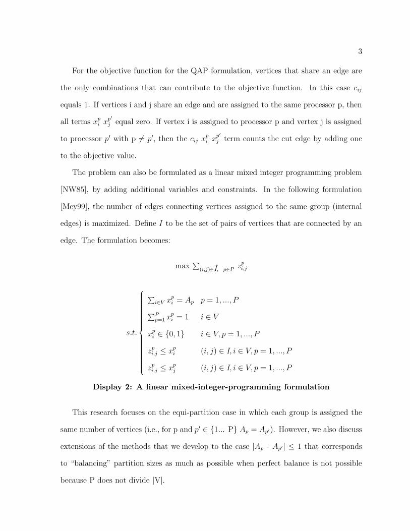
The problem can also be formulated as a linear mixed integer programming problem
[NW85], by adding additional variables and constraints. In the following formulation
[Mey99], the number of edges connecting vertices assigned to the same group (internal
edges) is maximized. Define I to be the set of pairs of vertices that are connected by an
edge. The formulation becomes:
max∑
(i,j)∈I, p∈Pz
pi,j
s.t.
∑
i∈V xpi = Ap p = 1, ..., P
∑Pp=1 x
pi = 1 i ∈ V
xpi ∈ 0, 1 i ∈ V, p = 1, ..., P
zpi,j ≤ x
pi (i, j) ∈ I, i ∈ V, p = 1, ..., P
zpi,j ≤ x
pj (i, j) ∈ I, i ∈ V, p = 1, ..., P
Display 2: A linear mixed-integer-programming formulation
This research focuses on the equi-partition case in which each group is assigned the
same number of vertices (i.e., for p and p′ ∈ 1... P Ap = Ap′). However, we also discuss
extensions of the methods that we develop to the case |Ap - Ap′| ≤ 1 that corresponds
to “balancing” partition sizes as much as possible when perfect balance is not possible
because P does not divide |V|.

4
1.2.2 Minimum Perimeter Formulation
Christou and Meyer [CM96] consider a geometric way of formulating this problem, which
is useful in terms of generating lower bounds on the optimal value. Figure 2 gives an
example of how the original graph is transformed into a domain of cells. Each vertex in
the graph becomes a cell (of unit area) and each edge becomes a boundary edge between
two cells (domain boundary edges are added as needed to provide four edges for each
cell). This geometric view is also the most natural representation of the PDE, vision,
and DB applications.
1 2 3 4 5 6
7 8 9 10 1211
13 14 15 16 17
1 2 3 4 5 6
7 8 9 10 11 12
13 14 15 16 17
Figure 2: The original graph and the geometric problem.
For the transformed problem, instead of counting cut edges, the sum of the perimeters
of the associated components is minimized. Formally, the problem to be solved is:
minimize∑
i Perim(Ci)
s.t.
each cell is assigned to one processor, and
each processor is assigned an equal number of cells,

5
where Perim(Ci) equals the perimeter for component Ci.
The relationship between cut edges and the total perimeter is:
cut edges = (total perimeter - perimeter of the boundary of the domain)/2
Since the perimeter of the boundary is a constant, minimizing perimeter is equivalent
to minimizing cut edges. Figure 3 shows an example of this relationship.(It also illustrates
a case in which the component sizes differ by one, because the number of components
(six, in this case) does not divide the number of cells (17). Thus, five components are of
size three and one component is of size two.)
A B B
A A B C C
C
D
D D
EEF F F
A A B C C D
A B B C D D
F F F E E
Figure 3: The top figure shows the original graph partitioned. The bottom figure showsan equivalent partition of cells.
In this example the minimum number of cut edges equals 14. The corresponding sum
of the perimeters for the components is 46 which is in agreement with the relation above,
since the perimeter for the original domain is 18, yielding the number of cut edges as
(46-18)/2. The bottom figure is also an example of a stripe-based solution (to be defined
formally below; informally this means that components are confined to horizontal bands
6
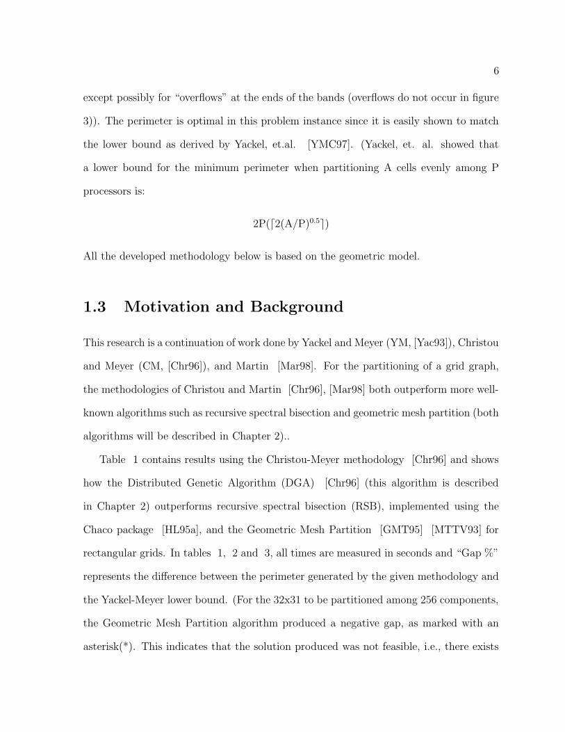
except possibly for “overflows” at the ends of the bands (overflows do not occur in figure
3)). The perimeter is optimal in this problem instance since it is easily shown to match
the lower bound as derived by Yackel, et.al. [YMC97]. (Yackel, et. al. showed that
a lower bound for the minimum perimeter when partitioning A cells evenly among P
processors is:
2P(d2(A/P)0.5e)
All the developed methodology below is based on the geometric model.
1.3 Motivation and Background
This research is a continuation of work done by Yackel and Meyer (YM, [Yac93]), Christou
and Meyer (CM, [Chr96]), and Martin [Mar98]. For the partitioning of a grid graph,
the methodologies of Christou and Martin [Chr96], [Mar98] both outperform more well-
known algorithms such as recursive spectral bisection and geometric mesh partition (both
algorithms will be described in Chapter 2)..
Table 1 contains results using the Christou-Meyer methodology [Chr96] and shows
how the Distributed Genetic Algorithm (DGA) [Chr96] (this algorithm is described
in Chapter 2) outperforms recursive spectral bisection (RSB), implemented using the
Chaco package [HL95a], and the Geometric Mesh Partition [GMT95] [MTTV93] for
rectangular grids. In tables 1, 2 and 3, all times are measured in seconds and “Gap %”
represents the difference between the perimeter generated by the given methodology and
the Yackel-Meyer lower bound. (For the 32x31 to be partitioned among 256 components,
the Geometric Mesh Partition algorithm produced a negative gap, as marked with an
asterisk(*). This indicates that the solution produced was not feasible, i.e., there exists

7
Time Gap %Time Gap % Time Gap %M x N P
32 x 31 8 1.8 6.52 43.6 5.43 6.9 1.08
32 x 31 256 4.3 6.73 152.3 -2.73* 7.1 0.00
32 x 30 64 3.0 6.25 90.4 6.25 7.8 0.00
100 x 100 8 9.0 9.33 111.0 7.39 17.7 2.28
128 x 128 128 85.5 14.13 539.9 7.13 15.5 1.63
256 x 256 256 227.8 13.25 3304.2 4.15 36.9 0.00
512 x 512 512 - - - - 123.8 0.56
Problem RSB GEOMETRIC DGA
Table 1: Christou-Meyer versus other graph-partitioning algorithms for rectangular grids
at least one component that was assigned at least two cells more than at least one other
component.) For more information about the chosen set of problems see [Chr96].
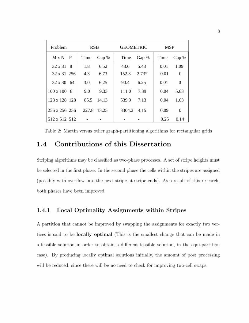
Martin [Mar98] also studied rectangular grids and obtained the results contained in
table 2, via a knapsack method for stripe height selection. In all cases, both Christou
and Martin [Chr96], [Mar98] did much better than the other methodologies. Christou
[Chr96] also studied non-rectangular grids. Table 3 contains those results.
When looking at table 3, for Christou’s methodology [Chr96] if the number of cells
within the overall grid is held constant as the number of cells to be assigned to each
component increases, performance decreases. Intuitively, this makes sense, since it is
harder to assign a small number of bigger groups near-optimally than it is to assign a
large number of smaller groups of cells near-optimally.
While the methodologies of Christou-Meyer and Martin [Chr96], [Mar98] outper-
formed the other methods, both methodologies have shortcomings (to be discussed later)
that are eliminated by the results in this dissertation.
8
Time Gap %Time Gap % Time Gap %M x N P
Problem RSB GEOMETRIC MSP
32 x 31 8 1.8 6.52 43.6 5.43 0.01 1.09
32 x 30 64 3.0 6.25 90.4 6.25 0.01 0
128 x 128 128 85.5 14.13 539.9 7.13 0.04 1.63
256 x 256 256 227.8 13.25 3304.2 4.15 0.09 0
32 x 31 256 4.3 6.73 152.3 -2.73* 0.01 0
512 x 512 512 - - - - 0.25 0.14
100 x 100 8 9.0 9.33 111.0 7.39 0.04 5.63
Table 2: Martin versus other graph-partitioning algorithms for rectangular grids
1.4 Contributions of this Dissertation
Striping algorithms may be classified as two-phase processes. A set of stripe heights must
be selected in the first phase. In the second phase the cells within the stripes are assigned
(possibly with overflow into the next stripe at stripe ends). As a result of this research,
both phases have been improved.
1.4.1 Local Optimality Assignments within Stripes
A partition that cannot be improved by swapping the assignments for exactly two ver-
tices is said to be locally optimal (This is the smallest change that can be made in
a feasible solution in order to obtain a different feasible solution, in the equi-partition
case). By producing locally optimal solutions initially, the amount of post processing
will be reduced, since there will be no need to check for improving two-cell swaps.

9
Time Gap %Time Gap % Time Gap %Shape P
Problem RSA
circle 16 23.3 24.44 9.1 21.80 19.8 8.33
torus 64 36.5 22.86 18.5 34.3 17.2
ellipsis 16 2.3 10.83 1.4 13.33 8.3 8.33
ellipsis 64 3.5 5.16 2.2 15.10 9.4 5.36
torus 16 27.3 28.97 12.5 32.67 18.8 11.50
diamond 16 14.0 38.67 6.5 35.74 10.7 16.40
diamond 64 18.7 29.78 9.0 28.80 16.2 13.37
11.00
RSQ DGA
circle 64 34.7 16.87 14.5 28.34 19.4 5.87
Table 3: Christou-Meyer versus other graph-partitioning algorithms for non-rectangulargrids
By identifying conditions under which local optimality is achieved by greedy assign-
ment procedures, a suite of alternative stripe-assigning procedures was developed to re-
duce undesirable assignments. While a given stripe-assigning procedure will not always
produce a good assignment, for most instances, at least one of the procedures within the
suite will work well.
1.4.2 Stripe-Height Selection
The bottleneck in all earlier striping algorithms was the stripe-height selection process.
For these methods to obtain the best solution, at least a super-polynomial amount of
time would potentially be required. An algorithm will be presented that produces an
optimal set of stripe heights in polynomial time.

10
1.5 Organization of this Dissertation
In Chapter 2, an overview of the methodology of this dissertation will be presented, along
with short descriptions of some well-known or related algorithms. Chapter 3 presents
three algorithms that produce locally optimal solutions. Chapter 4 shows how a grid
graph may be broken into a series of smaller and independent subproblems. Chapter 5
describes how to select the optimal set of stripe heights for a given assignment procedure.
Chapter 6 contains results and comparisons with some previous methodology. Chapter
7 contains concluding remarks and directions for future work.

11
Chapter 2
Background and Related Work
2.1 Introduction
Unless the graph is small, standard branch-and-bound techniques aren’t very useful for
partitioning a graph. The amount of computing resources required grows far too quickly.
Using AMPL [FGK93] to formulate the problem and CPLEX [Fra99]to solve it, the
software can reasonably handle at most the case of a 5 x 5 grid to be partitioned among
five components. For problems larger than this, the branch-and-bound trees get too large
to handle. Space and time become limiting factors.
Several heuristics have been devised for discovering good, if not optimal, solutions.
The algorithms to be discussed can be roughly broken into two groups: stripe-based and
non-stripe-based. The algorithms resulting from the research presented in this disserta-
tion, along with the related predecessor algorithms, fall into the category of stripe-based
methods. The other algorithms fall into the class of non-stripe-based methods.
A general description of the stripe assignment procedures (defined in Chapter 3) used
by Donaldson-Meyer (DM) and the formulation of stripe-height selection as a shortest-
path problem or as a dynamic-programming problem will be presented. The latter two
formulations suggest algorithms that exploit the presence of overlapping subproblems
within the solution in order to eliminate redundant calculations. These two formulations
are basically equivalent, except for the organization of data for the subproblems. The

12
end result is that both find the best stripe-based solution in polynomial time (although,
only the run-time for the dynamic-programming based solution will be presented).
2.2 Non-Striping Partitioning Algorithms
Four algorithms will be presented in this section: Kernighan-Lin, Recursive-spectral
Bisection, Geometric Mesh Partitioning, and METIS. None of these algorithms take ad-
vantage of known geometric properties of a graph (Geometric Mesh Partitioning assumes
that vertices that are far apart in euclidean distance probably don’t have an edge con-
necting the two vertices.). This is the main difference between the non-striping and
striping algorithms.
2.2.1 Kernighan-Lin
A well-known graph partitioning algorithm is due to Kernighan and Lin [KL70] [Chr96].
The algorithm divides the vertices into two groups and then looks for sequences of swaps
of vertices that reduce the number of cut edges. Within this sequence of swaps, it is
possible that a swap could be made that increases the number of cut edges, but leads to
later swaps that produce a net improvement in the number of cut edges. This algorithm
can lead to a locally optimal solution.
Kernighan and Lin proposed a way of getting away from a locally optimal solution.
Assume that the original graph has been partitioned into two groups: A and B. Within
both groups, recursively run the algorithm and identify groups A1 and A2, subgroups of
A, and B1 and B2, subgroups of B. The algorithm can then be run again using some
combination of subgroups as an initial partition.

13
2.2.2 Geometric Mesh Partition
The method of Miller, Teng, Thurston, and Vavasisi [GMT95], [MTTV93] differs from the
other non-striping algorithms in that this algorithm doesn’t use the adjacency information
of a graph to partition the graph. Instead this algorithm partitions the vertices of a graph
using only the physical location of vertices as the deciding factor. When describing the
algorithm, the ideas will be presented using two- and three-dimensional terms, but the
methodology is applicable for higher dimensions.
Geometric Mesh Partition Algorithm (Additional discussion about individual
steps follows the description of the algorithm.)
Input - The (x,y) coordinates for every vertex in the graph.
Output - The vertices in the original graph are divided into three sets:A,B, and C,
where A and B don’t share an edge and C is a set that when removed disconnects all
paths from A to B.
Algorithm
1. Map the points from R2 onto a unit sphere in R3.
2. Determine the centerpoint (defined below) for the points in R3.
3. Rotate and scale the points so that the centerpoint is at the
the origin.
4. Find a cutting plane that goes through the centerpoint.
5. Project down to R2 the points and cutting plane from step 4
6. Determine sets A, B, and C
For step 1, for a given (x,y) pair in R2, this point is mapped to (x,y,0) in R3. The cor-
responding point on the unit sphere is calculated by projecting along the line determined
by (x,y,0) and (0,0,1).

14
For step 2, the centerpoint is defined to be a point such that every plane through that
point divides the points into approximately equally sized groups. The authors [GMT95]
state that every set of points contains a centerpoint and the centerpoint can be found
using linear programming.
For step 4, the cutting plane defines a “Great Circle” that lies on the the sphere and
goes through the origin.
For step 5, the authors use several factors for partitioning the vertices into the three
groups. In the actual inplementation, the vertices are divided into only groups A and B,
thus creating an edge-separating set.
Although the algorithm doesn’t use any edge information, the authors [GMT95] apply
the methodology in a way so as to glean some edge information. Instead of calculating
the centerpoint, the authors calculate a “pseudo-centerpoint”. This is done by using a
sample of points to calculate a “centerpoint”. For this calculated centerpoint, several
cutting planes are generated. The cutting plane that performs the best is the one that
is used.
2.2.3 Recursive Spectral Bisection
Recursive spectral bisection describes a class of algorithms that follow the general form
[ST93]:
Function Recursive Bisection
Input - A graph G = (V,E) and p = number of groups (p = 2n)

15
1. Find an “optimal” bisection, G′ and G′′ of G.
2. While (| G′ | > |V|/p)
Perform Recursive Bisection(G′)
Perform Recursive Bisection(G′′)
3. Return the subgraphs G1,G2, ... , Gp
Finding an “Optimal” Partition: Spectral Bisection
Assume that the graph G = (V,E) is to be partitioned. For every vertex vi in V
create a new variable xi that may assume the values 1, -1. If xi is not equal to xj, then
vi is not in the same group as vj. The problem of finding the minumum number of cut
edges for partitioning a graph into two parts can be modeled as the following quadratic
program [HL95b], [Chr96].
min 14
∑
(i,j)∈E (xi - xj)2
s.t.
∑|V |i=1 xi = 0 (1)
xi ∈ −1, 1 i = 1..|V | (2)
Define L, the Laplacian matrix of the graph, to be:
Li,j =
−1 if (i, j) ∈ E
di if i = j
0 otherwise,
where di is the degree of of vertex vi. The matrix L = D - A, where D is a matrix
such that Dii equals the degree of vi and all other entries are zero, and A is the adjacency
matrix of G. The matrices D, A and the previous objective function are related as follows:

16
∑
(i,j)∈E (xi - xj)2 =
∑
(i,j)∈E(x2i + x2
j) - 2∑
(i,j)∈E xixj
=∑
(i,j)∈E 2 - x′Ax
= x′Dx - x′Ax
= x′Lx.
The original quadratic problem then becomes:
min 14
x′Lx
s.t.
x′e = 0 (1)
xi ∈ −1, 1 i = 1..|V | (2)
This problem is NP-Complete.
In the previous problem, constraint (2) can be relaxed producing a new problem
that has a known solution. In the previous formulation, if constraint (2) is replaced by
the constraint x′x = n, the optimal solution for the relaxed problem is x =√
n(second
normalized eigenvector of L) (this result was stated in [HL95b]). This produces x ∈ Rn,
but the components of x may not be feasible for the original quadratic problem.
To generate a feasible point, first, the median of the components of x is calculated.
For each component of x, if xi is greater than the median, then the corresponding vertex
is assigned to group 1; otherwise, the vertex is assigned to group 2. Some evening out of
the groups may be required, to obtain partitions of equal size.
2.2.4 METIS
METIS is the name of the software implementation of the methodology of Karypis and
Kumar [KK95c], [KK95a], [KK95d]. A high-level view of the methodology is:
17
1. Collapse the original graph down to a smaller graph through
a series of matchings. Matched vertices are combined as a single
vertex as are the corresponding set of edges that were incident
to the vertices.
2. Partition the reduced graph (for example, by spectral bisection).
3. Expand out the smaller graph, while maintaining the general
partition created in step 2.
After step 1, one vertex may represent several vertices. If vertex v is is one of the
vertices in the final collapsed graph and is assigned to group 1, then all of the vertices
that v represents are initially assigned to group 1. The speed of this algorithm comes
from the fact that size of the graph that is actually partitioned may be substanially
smaller than the original graph. At each phase of expansion, reassignment of vertices
may take place.
In the actual implementation of METIS, the authors implement four different algo-
rithms for partitioning a graph. Three of the algorithms are based on graph growing
heuristics. The other algorithm is based on spectral bisection. The authors evaluate the
performance of the different algorithms in [KK95b].
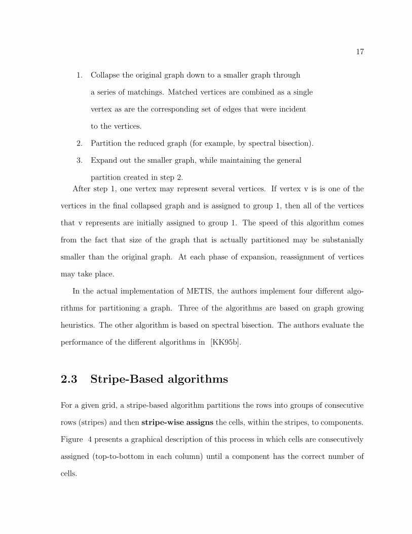
2.3 Stripe-Based algorithms
For a given grid, a stripe-based algorithm partitions the rows into groups of consecutive
rows (stripes) and then stripe-wise assigns the cells, within the stripes, to components.
Figure 4 presents a graphical description of this process in which cells are consecutively
assigned (top-to-bottom in each column) until a component has the correct number of
cells.

18
Original Grid
Striping the grid
Assigning cells within a stripe
Figure 4: Stripe-based assignment of a grid.

19
An optimal component is defined to be a component whose perimeter equals the
minimum perimeter required to enclosed the corresponding number of cells (area). Yackel
and Meyer showed that for every given number of cells a rectangle, with possibly at most
two fringe columns (columns that contain fewer assigned cells than all the other columns,
except perhaps for another fringe column), is an optimal component. A stripe height is
said to be optimal if optimal components can be assigned within the stripes.
For optimal or near-optimal stripe heights, stripe-based fill procedures produce opti-
mal or near-optimal components (in most cases, more on this later). This follows from
the fact that the stripes provide an easy way to assign rectangularly-shaped components.
This discovery of organizing the assignments into stripes came about from the use of
genetic algorithms for generating feasible solutions.
2.3.1 Stripe Assignments based on Genetic Algorithms
Both the methodology of Yackel-Meyer and of Christou-Meyer use a genetic-algorithm
heuristics [Gol89] [Hol92] [Mic94] for generating feasible solutions. Genetic algorithms
create a new set of feasible solutions from a parent set. The interactions of combining
parts of two feasible solutions (crossover) or changing part of a feasible solution (muta-
tion) are used to generate new feasible solutions. Both Yackel-Meyer and Christou-Meyer
then add in a decision-making policy for throwing out certain feasible solutions (survival
policies).
The major difference in the methodologies of Yackel-Meyer and Christou-Meyer is
how the elements of the feasible set of solutions are discovered. For Yackel-Meyer, there
is a single processor (host) that maintains the current set of feasible solutions. The host
node distributes work to the “node” processors. For Christou-Meyer, each node works

20
on its own set of feasible solutions. The nodes interact when the processor broadcasts a
set of feasible solutions to the other processors and then receives sets of solutions from
the other processors.
2.3.2 Yackel-Meyer Algorithm
Yackel and Meyer implemented a parallel version of a genetic algorithm. In this model,
there are two types of processors: host and node. The host processor coordinates ac-
tivities by sending out pairs of feasible solutions to node processors. A node processes
the feasible solutions via crossover to produce a pair of offspring. The offspring are then
mutated. A pair of solutions (selected from the two parents and two offspring) is then
passed back to the host processor. The process continues until stopped by a limit on the
number of iterations or if the lower bound is hit. The user is not guaranteed an optimal
solution, unless a feasible solution that matches the lower bound is found.
2.3.3 Christou-Meyer Algorithm
Christou and Meyer used several different ways for generating feasible solutions (a ran-
domized method for generating stripe heights and methods based on genetic algorithms).
The results generated using a distributed genetic algorithm produced the best overall re-
sults and will be discussed here.
Christou and Meyer eliminate the need for a host processor. From a very high-
level point of view, Christou-Meyer starts up a certain number of sibling processes each
of which generates a set of feasible solutions. At each node, certain members of the
feasible set are mated (and on certain individuals other genetic operations are applied).
Periodically, each process selects individuals to share with other processes and receives

21
individuals from other processes. This loop continues for some specified amount of time.
Christou and Meyer showed that any grid with enough rows can be partitioned into
stripes that allow the assignment of components that are of optimal or near-optimal
perimeter, as defined by Yackel and Meyer (see lemma 3 in [Chr96]). It follows that for
a large group of grid graphs, the vast majority of components will have perimeters at or
near optimal value. Figure 5 illustrates this point.
In figure 5, those components labeled I (I is for interior-to-stripe) are at or near
optimal perimeter. The unmarked components may be far from optimal. If the growth
in the perimeters for the unmarked components can be controlled, the total perimeter
for the grid will be very good. Intuitively, it seems reasonable that this striping method-
ology should produce very good results. Christou and Meyer have proven, under mild
assumption, that stripe-based solutions asymptotically approach (from the standpoint of
relative error) the optimal perimeter.
In particular, Christou and Meyer showed under mild assumptions (for MxN rectan-
gular grids partitioned among P components) that the relative difference between the
observed performance and the optimal partition (defined as δ below) is bounded from
above as follows:
δ < 1A0.5
p
+ 1Ap
.
As Ap, the number of cells assigned to component p, tends to infinity(as also does the
number of cells in the grid), then the relative difference goes to zero. For more details,
see Chapter 3 (Theorem 8) in this dissertation or Chapter 2 in [Chr96].

22
I
I I I
I I I I I
I I I I
I I
I
Figure 5: Interior-to-stripe (I) components at or near optimal perimeter

23
2.3.4 Knapsack Algorithm
Garey and Johnson in [GJ79] discuss the Knapsack problem and show it is an NP-
Complete problem. The following definition was taken from page 134 of [GJ79]:
Given : Given a finite set of items, U, such that each u ∈ U has an associated size
s(u) ∈ Z+ and value v(u) ∈ Z+ and a positive knapsack capacity B ≥ max s(u): u ∈
U.
Solve
max∑
u∈U v(u)
∑
u∈U s(u) ≤ B
Martin [Mar98] converts the stripe partitioning problem into a slight variant of the
Knapsack problem. In this variant formulation, the sum of the weights must equal B
(Martin also solves the minimization version of this problem.). This alternate problem
is also NP-Hard, since the original Knapsack problem can be reduced to this modified
Knapsack Problem by adding a slack variable.
Martin used software [MT90] that required that the problem be in standard form
(i.e. the constraint being an inequality). For a restricted set of inputs, Martin showed
that the solution of the problem in standard form satisfied the inequality constraint as
an equality. Because of this restriction on the inputs, we do not know if the problem
that Martin solved is NP-Hard.
For Martin’s algorithm only rectangular grids are considered. Only stripe heights
corresponding to an integral number of components are allowed. (That is, components
are not allowed to overflow from one stripe into the next.) Because of these assumptions,
the author is able to take advantage of certain features of the original graph. For a more
detailed discussion of the material that follows see Chapter 5.
24
For each valid stripe height, there is a unique perimeter (the objective coefficients
in the previous narrative) determined by adding the perimeters of the components as-
sociated with the height (the s(u)’s in the previous narrative). Since the domain is a
rectangle, for a given stripe height, no matter where these rows appear within the grid,
the same number of cells will occur in the stripe. It follows that for a feasible solution,
the order of the stripe heights doesn’t matter and the number of feasible solutions in-
volves counting combinations, rather than permutations. However, the total number of
solutions is at least super polynomial, as will be proved in Chapter 5.
2.3.5 The Shortest-Path/Dynamic-Programming Approach
Both methods are based on the fact that, under certain assumptions, two row indices
of the grid and a direction of assignment can be used to divide the original problem
into two problems that are identical in nature to the original problem, but which can be
solved independently of one another. (These two smaller problems will be referred to as
subproblems throughout the remainder of this dissertation) The ability to divide the
original problem into similar, but independent problems, is the single most important
tool in the discovery of polynomial-time algorithms for determining the best stripe-based
solution.
Although there are two algorithms presented, the only real difference between the
methods is how the the data for subproblems are organized.

25
2.4 Improved Stripe Assignment
Donaldson and Meyer [Don97] show that under certain circumstances a modified version
of the Christou-Meyer fill produces a locally optimal solution for a rectangular grid. Don-
aldson and Meyer also present two algorithms that can produce locally-optimal solutions
for a larger class of grids.
Initial experimentation using a slight variation of one of the locally-optimal algorithms
(the Improved U-turn Algorithm, see Chapter 3) did not produce very good results. As a
result, research into different assigning procedures was conducted that produced a set of
nine different assignment methods for the cells that are assigned to components appearing
in more than one stripe. This multi-heuristic approach produced very good results.
2.5 Summary
When looking at a stripe-based method two areas for concern appear. Assignments of
components that cross stripe boundaries can add significantly to the total perimeter of
the domain. Poorly chosen stripe-heights can also drastically affect the total perimeter.
Methods that address these two issues are the two main areas of focus for the remainder
of this dissertation.
Throughout the remainder of this dissertation, references will be made to the work
of Yackel-Meyer and Christou-Meyer. Rather than write out the full names, when the
work of Yackel and Meyer is being referred to, YM will be used. In the case of Christou
and Meyer, CM will be used.

26
Chapter 3
Improved Stripe Assignment
3.1 Introduction
In earlier research, Yackel-Meyer (YM) and Christou-Meyer (CM) were able to produce
very good results using striping techniques. Nothing was known about the possibilities
for improvement via swapping (although, in their implementation, CM used a post-
processing swap phase). In particular, it was not known under what conditions when
pairs of cells could have their assignments swapped with the result being an improved
total perimeter.
The first result of this research shows that under certain conditions (including rect-
angular origin domain) CM does produce a locally optimal solution (i.e., an assignment
that can’t be improved by reassigning two cells). Local optimality is clearly desirable
from a theoretical viewpoint. It is also computationally desirable since it eliminates the
need for a post-processing swap phase. It will also be shown that CM can also make
assignments that are far from locally optimal, if certain conditions are not satisfied.
We now discuss the Basic U-turn algorithm, and show that it makes assignments
that are guaranteed to be locally optimal for all cases of rectangular grids. This method
can be extended to a more elaborate algorithm, the Improved U-turn algorithm. The Im-
proved U-turn algorithm will be briefly discussed but the proof of its local optimality
will only be sketched.

27
The concept of a U-turn region (to be defined later) arose initially as we considered the
area within an assignment where swap improvements could be made. As mentioned in the
previous chapter, YM and CM make assignments such that the majority of components
have optimal or near-optimal perimeters. However, large deviations from optimality
occurred when trying to assign components at the boundary of the domain. The research
presented in this chapter is designed to reduce the effects of these boundary components.
Two factors were examined to reduce the ill effects of a poor assignment within the
U-turn region. The first was an improvement of the CM method called the Basic U-
turn algorithm. The second factor involved increasing the size of the U-turn region and
developing assignment patterns that would be better suited to handle certain situations
(the Improved U-turn algorithm). The reader should notice that by expanding the U-
turn region, components that would have been assigned in near-optimal patterns may
no longer be, so a balance between the size of the U-turn region and the number of
well-shaped components had to be achieved.
Local optimality of a fill procedure is proved only in the case of rectangular domains.
However, the ideas developed in conjunction with the proof are useful in terms of devel-
oping good fill procedures for more general domains as we will see in Chapter 6.
The U-turn region also provided a completely unexpected result. This region in the
grid provided a convenient method of dividing the grid into independent parts. This
ability to divide the grid into independent parts is the foundation upon which the second
major breakthrough of the research is built. This led to the discovery of a polynomial
algorithm that produces the best stripe-based solution for a given fill procedure.

28
3.2 Terms and Definitions
In this chapter, only rectangular grids will be considered. Examples of a rectangular
and a non-rectangular grid are given in figure 6.
Rectangular Grid
Non-rectangular Grid
Figure 6: A rectangular and a non-rectangular grid
Definition - A stripe is defined to be any collection of consecutive rows within a
grid.
Definition - A component is any collection of cells assigned to the same group (or
processor). Figure 7 shows a component assigned to group A.

29
Definition - The process of assigning the cells within a stripe is called stripe as-
signment.
Definition - For this discussion, a solution is said to be locally optimal if the overall
perimeter can’t be reduced by swapping the assignments for two cells.
Definition - Swapping the assignments for two cells will be referred to as a two-cell
swap. (We focus on the balanced case in which components have equal area. In this
case the smallest change that can produce another feasible solution is a two-cell swap).
Figure 7 will be used to demonstrate several definitions.
In figure 7, we assume that the cells shown represent all the cells assigned to compo-
nent A and categorize the cells according to their contribution to the total perimeter of
the component.
Definition - An interior cell is assigned to the same component as all four of its
neighbors. In figure 7, interior cells are marked as 0.
Definition - An edge cell contributes one to the perimeter. These cells are marked
with a 1 in figure 7.
Definition - A vertex cell is a corner cell in a component or a cell with exactly two
neighbors assigned to its component. These cells are marked with 2’s. Type 2 cells may
also occur in “peninsulas”. These are marked with 2∗ in figure 7.
Definition - A spike cell is a cell that has only a single neighbor assigned to the
same processor. This cell is marked with a 3.
Definition - An island cell is assigned to a different processor than all of its neigh-
bors. An example of this is marked with a 4. (In the constructions to follow, island cells
are not generated)
Definition - In figure 7 those cells marked as 2∗ and 3∗ make up a peninsula. A
peninsula is a connected collection of cells with the property that all cells in it are type-2

30
A A A A A A
A A A A
A A A A
A A A A
A
A
2 1 1 1 3 4
1 0 0 1
1 0 0 1
1 1 1 2
2*
3*
Figure 7: Classification of cell assignments by perimeter contribution

31
or 3.
Definition - Boundary cells are those cells that are of types 1 through 3
Definition - Semi-perimeter equals the sum of the number of rows and columns
occupied by a component.
Definition - The enclosing frame (also known as the rectangular hull or enclos-
ing rectangle) for a connected component is the minimum sized rectangle that encloses
the component.
Definition - If a component is not a rectangle, but can be represented as the union
of a rectangle plus additional incomplete “boundary” rows or columns, then the cells in
these “boundary” rows or columns are fringe cells.
Definition - A component is said to be slice convex if for any two cells within a
row or column of a component, all the cells within the row or column between these two
cells are assigned to the component.
Definition - For a component C, a gap occurs within a column (or row) if there
are two cells, a and b, assigned to C within that column (or row), and one or more cells
between a and b that are not assigned to C (between a and b there are no other cells
assigned to C). Figure 10 shows examples of interior and boundary gaps.
Definition - A component is said to be top-to-bottom column-wise assigned if, with
the rows numbered top to bottom and the columns numbered left to right, within column
j, cell[i][j] is assigned before cell[i+1][j] and cells in column j will be assigned before cells
in column j-1 (when assigning right to left) or j+1 (when assigning left to right).
Definition - To row-wise assign a component is to assign all cells in row i, either
left to right or right to left, within certain columns, before assigning any cells in row i+1.
32
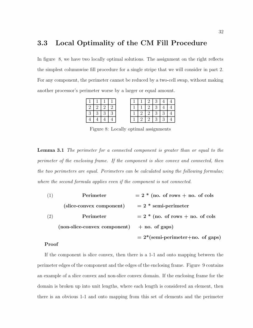
3.3 Local Optimality of the CM Fill Procedure
In figure 8, we have two locally optimal solutions. The assignment on the right reflects
the simplest columnwise fill procedure for a single stripe that we will consider in part 2.
For any component, the perimeter cannot be reduced by a two-cell swap, without making
another processor’s perimeter worse by a larger or equal amount.
1 1 1 1 1 1 2 3 4 42 2 2 2 1 1 2 3 4 43 3 3 3 1 2 2 3 3 44 4 4 4 1 2 2 3 3 4
Figure 8: Locally optimal assignments
Lemma 3.1 The perimeter for a connected component is greater than or equal to the
perimeter of the enclosing frame. If the component is slice convex and connected, then
the two perimeters are equal. Perimeters can be calculated using the following formulas;
where the second formula applies even if the component is not connected.
(1) Perimeter = 2 * (no. of rows + no. of cols
(slice-convex component) = 2 * semi-perimeter
(2) Perimeter = 2 * (no. of rows + no. of cols
(non-slice-convex component) + no. of gaps)
= 2*(semi-perimeter+no. of gaps)
Proof
If the component is slice convex, then there is a 1-1 and onto mapping between the
perimeter edges of the component and the edges of the enclosing frame. Figure 9 contains
an example of a slice convex and non-slice convex domain. If the enclosing frame for the
domain is broken up into unit lengths, where each length is considered an element, then
there is an obvious 1-1 and onto mapping from this set of elements and the perimeter
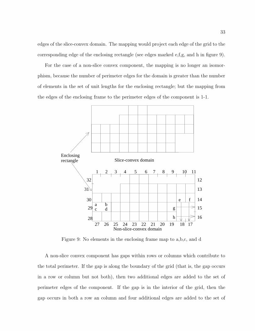
33
edges of the slice-convex domain. The mapping would project each edge of the grid to the
corresponding edge of the enclosing rectangle (see edges marked e,f,g, and h in figure 9).
For the case of a non-slice convex component, the mapping is no longer an isomor-
phism, because the number of perimeter edges for the domain is greater than the number
of elements in the set of unit lengths for the enclosing rectangle; but the mapping from
the edges of the enclosing frame to the perimeter edges of the component is 1-1.
Slice-convex domain
Non-slice-convex domain
Enclosingrectangle
1 2 3 4 5 6 7 8 9 10 11
12
13
14
15
16
171819202122232425262728
29
30
31
32
c da b
e f
g
h
Figure 9: No elements in the enclosing frame map to a,b,c, and d
A non-slice convex component has gaps within rows or columns which contribute to
the total perimeter. If the gap is along the boundary of the grid (that is, the gap occurs
in a row or column but not both), then two additional edges are added to the set of
perimeter edges of the component. If the gap is in the interior of the grid, then the
gap occurs in both a row an column and four additional edges are added to the set of

34
perimeter edges (see figure 10) (The gap count in Lemma 3.1 includes both row and
column gaps.).
2
A A A A A A A A
A A A A A A A
A A A A A A A A
Perimeter of enclosing rectangle = 2*(4+8) = 24
A A A A A A A
Perimeter = 2*(4+8) + 4 + 2 = 30
Figure 10: Perimeter for component with interior gap and boundary gap
Lemma 3.2 Adding a cell to a slice-convex component cannot decrease the perimeter.
Proof
Follows from Lemma 3.1, formulas 1 and 2, since semi-perimeter cannot decrease.
2
Lemma 3.3 The perimeter for a rectangular component can not be reduce by a two-cell
swap.
Proof (sketch) - Case 1, the component is assigned to either a single column or row
(see any of the components in the lefthand picture in figure 8). Moving a corner cell will
reduce the number of rows or columns by one, but will increase the number of columns
or rows by one. There is no improvement. Moving an interior cell increases the overall
perimeter.

35
Case 2 - The component appears in multiple rows and columns. Moving a cell will
not reduce the number of rows or columns, because each row and column contained more
than one cell. In fact, wherever the new assignment is made at least one column or row
will be added to the size of the enclosing frame.
2
In figure 11, we have a non-locally-optimal solution. Here the boldfaced 3 and 4 can
be swapped and the overall perimeter will be reduced. In this case, moving the 3 reduces
the number of columns by one. Moving the 4 to 3’s old position doesn’t make worse 4’s
perimeter.
Lemma 3.4 Assuming slice convexity and no island cells, the only swap that can improve
the total perimeter is one in which a spike cell is moved to a corner destination (one with
vertical and horizontal neighbors in the same component).
Proof -
Moving a type-3 cell to a corner position will reduce semi-perimeter because its origin
was the only cell in its row or column and its destination is a position for which the
corresponding row and column are already included in the semi-perimeter.
Type-k cells, k = 2,1, or 0, either
1) have vertical and horizontal neighbors in their component, so corresponding loca-
tion swaps cannot reduce semi-perimeter; or
2) lie on a peninsula, in which case a swap produces a gap, and therefore, by the second
formula in lemma 3.1, this gap compensates for the row or column count decrement and
the perimeter cannot decrease.
2

36
1 1 1 2 2 21 1 1 2 2 21 1 1 2 2 21 1 3 3 2 2
4 4 4 3 3 34 4 4 3 3 34 4 4 4 3 3
Figure 11: A non-locally optimal assignment
In the original CM fill method, the actual columns were filled from the top. We will
show that a modified CM fill method will produce a locally optimal solution if certain
conditions are met, as indicated in the following theorem:
Theorem 3.1 Let the following assumptions be satisfied:
1. Graph partitioned using a stripe decomposition method.
2. Filling by column, alternate (down and up) fill directions.
(snake-fill procedure).
3. An integral number of processors is contained within each stripe.
4. Component area is ≥ 4.
5. 34
* component area ≥ the largest stripe height
Then the solution generated is locally optimal.
(In the discussion to follow, A will be used to denote the area or the number of cells
assigned to a component.)
The first three conditions are needed for defining the stripe assignment. The last two
are needed for technical reasons. If the area to be assigned to a component is 1, 2 or 3,
then any connected component is of minimum perimeter, so the assignments produced
by the fill procedure are actually optimal. So we only consider areas greater than or
equal to 4. As a consequence of assumption 5 we will show that there will never be spike
cells in consecutive columns.

37
(2/3 - e)s
(2/3 + e)s
(1/3-e)s
e*s
s
1 2 3 4
C C
D
D
D
Figure 12: Spike cells in non-consecutive columns
In figure 12 we have two components, C and D, with area equal to 4/3 of the stripe
height (The proof is analogous if A > 4/3*stripe height). If C is to have a spike in the
column labelled 2, then the number of C cells in column 2 must be greater than the
number of C cells in column 1. Thus, we assume that C contains (2/3 - ε)*s cells in
column 1 and (2/3 + ε)*s cells in column 2. The remainder of column 2 contains (1/3 -
ε)*s cells of D. Since D is also assigned an area equal to 4/3*s, there are s+ ε remaining
cells of D to be assigned. That means that all of the column labelled 3 and part of 4 will
contain D’s. Therefore, D cannot have a spike cell in column 3, and D and C cannot have
spike cells in consecutive columns (This prevents the following from happening: suppose
s > 3/4*A and as a result, there are no D cells in column 4, then the bottom D cell in
column 3 could be swapped with the top C cell in column 2, and the total perimeter
would be reduced.)
Observations
Fact 3.1 Assumption 2 guarantees that the cells for a given processor are connected.
This follows from the fact that the first cell assigned in the next column will be adjacent
to the last assigned cell in the current column.

38
Fact 3.2 The assignment is slice convex. This follows from the fill procedure. Within
column, the cells are assigned consecutively. Columns are filled from left to right, and
this implies that the row assignments are slice convex, since clearly this fill can produce
no gaps in a row.
Fact 3.3 It follows from Fact 3.1 and assumption 5 that no component will contain an
island cell.
Overview of Proof of Theorem 3.1 - The proof will be broken into several parts.
First, certain cells will be eliminated as possible candidates for swapping. Across-stripe
swaps will be shown to not improve the overall perimeter. Lastly, it will be shown that
no within-stripe swap will improve the overall perimeter.
In all cases, we will show that either:
1. The component has at least two cells within every row or column, which
means swapping will not reduce the number of rows or columns of
the component; or
2. The component has a single cell appearing in a row or column, in which
case swapping that cell assignment would increase the perimeter of the
other component.
B B* A*... B B* A* ...
B* A* A...
B* A* A
Figure 13: Boundary cells: B∗’s and A∗’s
The following lemma is useful.

39
Lemma 3.5 No swaps between non-adjacent components can improve the overall perime-
ter.
Proof - Follows from lemma 3.4..
2
This lemma implies that the only cells that could possibly produce a better solution
are those cells along the boundary between two adjacent areas.
Lemma 3.6 A swap across a stripe cannot improve the combined perimeter for the com-
ponents involved.
Proof -
Such a swap cannot have a corner cell as a destination, by lemma 3.4 there can be no
improving swap.
2
This lemma implies that only swaps of cells contained within the same stripe need be
considered.
It will now be shown that there does not exist a within-stripe swap that improves
the overall perimeter. If a swap were to improve the overall perimeter, for at least one of
the components the perimeter would have to decrease and for the other component the
perimeter would have to remain the same or decrease. (This follows from the fact for a
given component that the only increments for change in size of perimeter are a decrease
by 2, no change, and an increase by 2 or 4). Denote a component for which the size of
the perimeter decreases as “I” (for improving). A component for which the size of the
perimeter is at worst unchanged will be denoted by “N” (non-increasing).
In order to prove that there does not exist a within-stripe swap that reduces the overall
perimeter, it will be shown that there does not exist a pair of adjacent components one

40
of which is a N and the other is an I (called an I-N pair). Only adjacent regions need by
considered by lemma 3.5
Because of the hypothesis that stripe height is less than or equal to 0.75*component
area, a component cannot fit into a single column. Therefore, there are two cases that
must be examined:
1. I intersects at least three columns.
2. I intersects exactly two columns.
Case 1 - A three-column I component
I I N
? I N
. N
. N
. N
? I I
1 2 3 column labels
(Note: The ?’s indicate that the cell may or may not contain an I.)
Also assume that an N component appears in column labelled 3. Since there can be
no spikes in column labelled 2 because every cell in the column has at least two neighbors,
the only swaps that would reduce the size of the perimeter of I are those that move a
spike cell from column 1 or 3 to column 3 or 1. Assuming that a spike appears in column
3, then the swap to reduce I would not involve the N component. Therefore, this pair of
components can not be an I-N pair.
For the case that I intersects more than three columns the argument is analogous (the
only change is the number of columns completely assigned to I’s).

41
Case 2 - I is a two-column component. (this is relevant when 43*stripe height ≤ A ≤
2 * stripe height).
We have the following case:
I II IH I.. ?
I
1 2 3 column labels
Figure 14: I as a two-column component.
If A < 2*stripe height, by Lemma 3.4, if I’s perimeter is to be reduced, then the spike
cell must be moved to a corner position. In figure 14, that corner position is marked
with an H. Whatever component was originally assigned in position H does not appear
in column labelled 3. As a consequence of assumption 4, we know that cell H is not a
spike cell. So to swap I to position H will reduce I’s perimeter, but will also increase the
other component’s perimeter by an equal amount. Therefore, no overall improvement
occurs.
Again, in the previous argument, if the fringe is on the other side, the argument still
holds.
If A equals 2*stripe height, then all the components are rectangles and are at a local
minimum.
All possible configurations that the I component could have assumed have now been
checked, and no I-N improving swap is possible.
2
The left grid in figure 8 illustrates a local minimum of poor quality. In that example,
each component has a perimeter of 10, whereas an optimal solution uses 2x2 components

42
with perimeter equal to eight each.
However, if the CM method is applied with properly chosen stripe heights, good
solutions are obtained. If the grid is MxN and the grid is to be broken into P partitions,
then we have the following theorem based on constructing a feasible solution via a striping
approach of CM [CM95].
Theorem 8 (Christou-Meyer) - Assuming P divides MN and that P ≥ max (M,N)
the minimum perimeter problem MP (M,N,P) has a feasible solution whose relative
distance δ from the lower bound satisfies:
δ < 1A0.5
p
+ 1Ap
Thus the error bound δ converges to zero as Ap (the area of each processor) tends to
infinity.
3.4 Overflow Assignments
All the previous results are for rectangular grids that have been partitioned into stripes
that can be assigned to an integral number of components. How does the CM algorithm
handle the case that an integral number of components can’t be assigned within a stripe?
When a component overflows from one stripe to the next, CM row-wise assigns the
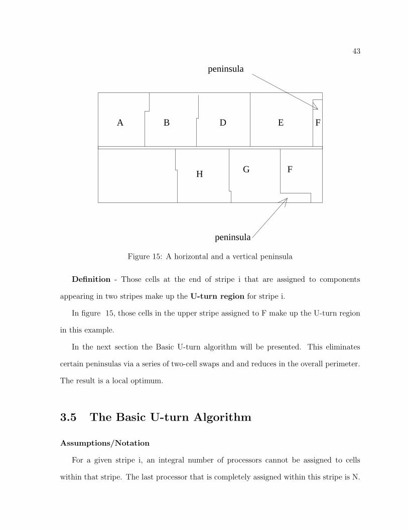
overflow cells. This can lead to the creation of peninsulas. Figure 15 shows two peninsula
examples.
Component G has a horizontal peninsula, and component F has a vertical peninsula.
Obviously, row-assigning the overflow cells does not always produce good assignments (to
improve the assignments the reader can think of “folding in” the peninsula like a blade
in a pocket knife). Column-assigning the cells can also produce peninsulas. We may now
formally define the region in which these overflow assignments occur.
43
A B D E F
FGH
peninsula
peninsula
Figure 15: A horizontal and a vertical peninsula
Definition - Those cells at the end of stripe i that are assigned to components
appearing in two stripes make up the U-turn region for stripe i.
In figure 15, those cells in the upper stripe assigned to F make up the U-turn region
in this example.
In the next section the Basic U-turn algorithm will be presented. This eliminates
certain peninsulas via a series of two-cell swaps and and reduces in the overall perimeter.
The result is a local optimum.
3.5 The Basic U-turn Algorithm
Assumptions/Notation
For a given stripe i, an integral number of processors cannot be assigned to cells
within that stripe. The last processor that is completely assigned within this stripe is N.

44
In the following algorithm, the direction of assignment is left to right; the arguments
can be suitably modified if the direction of assignment is right to left. All columns are
filled top-down (This is not a source of difficulty with respect to local optimum because
we assume stripe height < A/4.).
Overview of Algorithm
This algorithm can be broken into two parts. The first part is the initial columnwise
assignment of cells in the grid. The second part searchs the grid for pairwise swaps
that will reduce the overall perimeter. After all such swaps are identified and made, the
result is a locally optimal solution. In figure 16 assignments are made columnwise top to
bottom. The arrows indicate the direction of fill. Figures 17 and 18 show the kinds of
swaps that are made as needed (the reader may have noticed that an across-stripe swap
is a “vertical” slider swap).
Algorithm
Cells are assigned columnwise, top to bottom, unless indicated as exceptions below:
Step 1 - Assigning processor N (see figure 19), the non-overflow case.
while (the number of unassigned cells >= area)
- assign the cells for the processor columnwise top
to bottom.
Now assume that in figure 19, the unassigned area between columns j and s, inclusive,
in stripe i, is not large enough to accommodate another complete component with A cells
and thus is designated as the U-turn region.
The next processor to be assigned will overflow into the next stripe.

45
initial fill →
↓overflow
← fill
↓overflow
fill →
↓. overflow..
→ fill
↓overflow
fill ←
Figure 16: Flow of assignments

46
I I I I I I N N N N N N NI I I I I I N N N N N N N
Before
I I I I I I N N N N N N NI I I I I I N N N N N N N
O I I I I I I N N N N N N N
After
First swapSecond swap
O O O O O O O O O O O O O O OO O O O O O O O O O O O O O O
O O O O O O O O O O O O O O O
I I I I I I N N N N N N N O
Figure 17: An example of a pair of slider swaps

47
N N N N N N N N O
N N N N N N N O ON N N N N N N O O
O O OO OO O
Before
Swap
N N N N N N N O ON N N N N N N O O
O OO O
N N N N N N N O O
N O O
After
Figure 18: An example of an across-stripe swap
N N NStripe i N N N
↓. N. -. -
N N -
. j s
Figure 19: Assigning non-overflow component N

48
Step 2 - Assigning component O (see figure 20), the overflow case.
N N N O O OStripe i N N N O O
↓ .. N .. O O. O
N N O O
column labels s
- - - - - - O OStripe i+1 - - - - - - ↓ ↓
Figure 20: Assigning overflow component O
Assign all the remaining cells in stripe i to O.
while (there remain O’s to assign)
Assign the O’s top to bottom in stripe i+1.
if (column s, in both stripes, is not completely assigned
to O’s)
// Balance heights in column s-1 and s via reducing swaps
// (see figure 20).
for the stripe in which the O’s don’t completely fill
column s
while (height of O’s in column s-1) + 1 <
(height of O’s in column s)

49
swap the spike O with the lowest (highest) N (N’, if the
peninsula is in stripe i+1) in column s - 1.
// Taking care of the extra cell.
if (height of O’s in column s > height of O’s in column s-1)
if (stripe == i)
assign this extra cell in the last row of stripe i in
column s-2.
else
assign this extra cell in the first row of stripe i+1
in column s-2.
(Note: In figure 21, because of assumption 1 (stated below), the O in column s-2 can
never be a spike. See lemma 3.9 for details.)
Step 3 - Making reducing swaps.
At this point, the grid has been completely assigned. We refer to this assignment as
the initial assignment. For any pair of stripes, there can be at most one component

50
N N N N N N N N N NN N N N O N N N N NN N N N N N N
Stripe i N N . N N N O ON N . N N N O ON N . N N N O O
Z N N N N O Z N N O O Os s
Figure 21: Removing a peninsula via swaps
that appears in both stripes. There are two types of swaps that can improve the total
perimeter. The first is an across-stripe swap. The second is a slider multi-swap (referred
to below as simply a slider). A slider occurs when a component from stripe i+1 (i) has
a single cell in stripe i (i+1). Multi-swaps may involve several two-cell swaps. After
performing these swaps in Step 3, the assignment is locally optimal.
Step 3 - Making reducing swaps.
i = 1;
while ( i <= number of stripes - 1)
Step 4.1 - Check for across-stripe swap for components adjacent to overflow com-
ponents. Components assigned immediately after an O component are designated N’ For
the following block of code, refer to figures 22 and and figure 23.
N N N N N N O N N N N N O ON N N N N O O N N N N N O ON N N N N O O N N N N N O ON N N N N O O N N N N N O O
N’ N’ N’ O O O O N’ N’ N’ N O O ON’ N’ N’ N’ O O O N’ N’ N’ N’ O O O
Figure 22: An N-O across-stripe swap

51
N N N N O O O N N N N O O ON N N O O O O N N N N’ O O O
N’ N’ N’ N’ N’ O O N’ N’ N’ N’ N’ O OI N’ N’ N’ N’ O O I N’ N’ N’ N’ O OI N’ N’ N’ N’ O O I N’ N’ N’ N’ O OI N’ N’ N’ N’ N’ O I N’ N’ N’ N’ O O
m m
Figure 23: A O-N’ across-stripe swap
if (O has a side spike in stripe i(i+1)) &&
(O’s spike falls within the columns containing N) &&
(N(N’) has a rightside spike in stripe i+1(i))
- swap the two spikes.
At this point, N,O or N’ could have cells in both stripe i and i+1, but this is not true
for any other component appearing in either stripe.
Observe that across-stripe swaps for O result in full height rectangles in stripes i and
i+1 (and no O spikes), because these swaps have corner cells as destinations.
The last improving swap within stripe and is called a slider swap. This definition
will be demonstrated by an example, see figures 24 and 25 (Bottom slider swaps are
also possible, and are similar, hence are not illustrated here.).
stripe i 1 1 1 2 2 2 2 2 2 2 2 2 2 2 2 2
stripe i+1 5 5 5 5 4 4 4 4 4 3 3 3 3 3 3 26 5 5 5 5 4 4 4 4 4 3 3 3 3 3 36 5 5 5 5 4 4 4 4 4 3 3 3 3 3 36 5 5 5 5 4 4 4 4 4 3 3 3 3 3 36 5 5 5 5 4 4 4 4 4 3 3 3 3 3 3
Figure 24: Before a top slider (the bold 2 is the slider)

52
stripe i 1 1 1 2 2 2 2 2 2 2 2 2 2 2 2 2
stripe i+1 5 5 5 5 2 4 4 4 4 4 3 3 3 3 3 36 5 5 5 5 4 4 4 4 4 3 3 3 3 3 36 5 5 5 5 4 4 4 4 4 3 3 3 3 3 36 5 5 5 5 4 4 4 4 4 3 3 3 3 3 36 5 5 5 5 4 4 4 4 4 3 3 3 3 3 3
Figure 25: After a two top slider swaps
Step 4.2 - Check for a slider.
Search for a slider cell within each stripe.
Slide this cell by swapping as necessary.
(Several swaps may be required. )
// This ends the while ( i <= number of stripes - 1).loop
At this point, all of the components in stripe i have locally optimal perimeters.
Proof of Local Optimality
Assumptions
1. Area for each processor > 4*(smallest stripe height).
2. Stripe height ≥ 4.
3. Each stripe has at least 5 components.
Fact 3.4 A swap is only made if it reduces the overall perimeter.
We group the components into three types. The first, Type I (I is for interior), is
a component that is not a neighbor of an overflow component in the same stripe, at
the end of the initial assignment. The second type, Type O (O is for overflow), is a
component that does extend over two stripes at the end of the initial assignment (these

53
types of components will always span two stripes). The last component, Type N (N is
for neighbor), is a component that is a within-stripe neighbor to a Type O component.
To prove local optimality, we will show that no component can be improved via a
swap. Each type of component will be considered separately. When considering possible
swap cells, only destinations with assignments that match neighbors of spike cells need be
considered, since otherwise an island cell would result. We need the following definition:
Definition - For a given U-turn region, define those cells that are assigned to type-N
components, type-O components, and any other component that is involved in a slider
swap to be the swap area for the U-turn region.
We first need to prove that processing a U-turn region doesn’t result in a configuration
that would allow a chain reaction of other swaps. In order to prove this result, we need
the following lemma and associated definition.
Definition - A component in which a slider cell was detected will be termed a slider
component.
Lemma 3.7 There is at least one component in each stripe that cannot participate in a
slider swap.
Proof (by contradiction) - A slider component can either be a N-component or
an O-component. For this argument, assume that the slider components are N’s (the
argument for other cases is similar).
Assume that N and N’ (see figure 26) are slider components. Because of the as-
sumption about each stripe containing at least five components, it follows that neither
N and N’ can extend to the halfway column of the grid. From this it also follows there
there exists a component Is that neither component can affect. Also, N (N’) can’t affect
anything to the right (left) of Is. So it follows that two slider components cannot affect

54
common components.
By a similar argument, if N and N’ appear in consecutive stripes, then N (or N’)
cannot affect N’ (or N) (see figure 26).
We have now shown that both stripes within a swap area area cannot be affected by
any component outside the swap area.
2
This previous lemma is useful in that it shows that there is a termination point to the
slider swap. We also know that a N-component could never involve another N-component
from another U-turn region.
Slider componentN
Slider component
N’
UnaffectedUnaffected I_sby by
NN’
U-turnregion
Swap area for N’
U-turnregion
Swap area for N
Figure 26: Component Is can’t be affected by slider swaps.
N
N’
U-turnregion
U-turnregion
Figure 27: One slider component cannot affect another slider component.

55
This previous lemma is useful in that it shows that there is a termination point to the
slider swap. We also know that a N-component could never involve another N-component
from another U-turn region.
Lemma 3.8 The final total perimeter for the domain is independent of the order in
which the U-turn regions are processed.
Proof - From the previous lemma, we know that a slider swap in one region does not
change the assignment for a component in another swap area. The only other type of
swap is an across-stripe swap, which involves only O and either N or N’ component within
the U-turn region. It follows that the swap areas are mutually exclusive. Therefore, we
can process the U-turn regions in any order, without affecting the final solution.
2
Because of this lemma, we may processes the U-turn regions starting at the top of
the grid and working down, as was done in the algorithm.
It is important that the reader understand the necessity of the previous two lemmas.
The proofs that follow depend on potential spike positions being easily identified.
For the following proof, the direction of assignment is assumed to be left to right in
the stripe that could produce an overflow into the next stripe. The argument is similar
for the case of right-to-left assignment.
To prove the theorem, we must show that for each type of configuration that the
configuration cannot be improved whether or not the configuration had been involved
in some type of swap. Since the O-type configuration is where the swapping begins,
this is the configuration that will be dealt with first. First we need to state some facts
concerning slider swaps.
Facts concerning a slider swap

56
1
2
3
i
i+1
t
Swap
area
Swap
area
Swap
area
Swap
area
Swap
area
Swap
area
Figure 28: Mutually exclusive swap areas
1. The overflow for the slider component can only contain a
single cell (which forms a spike).
2. Any component that is improved as a result a slider will have
a rectangle for its final configuration.
3. A slider allows for across-component swaps.
Before we examine the O-component, we need the following lemma, which eliminates
possible spike positions.
Lemma 3.9 If the peninsula elimination procedure is applied to a component, then the
number of columns completely assigned to that component in the other stripe is at least
three.
Proof - By assumption 1, we know that component O has enough area to be assigned
to at least four columns, within one stripe. Since the peninsula elimination phase only
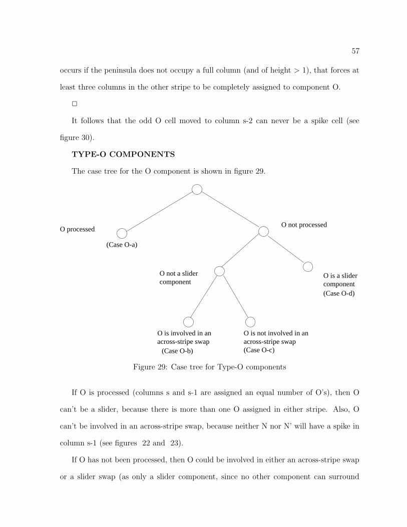
57
occurs if the peninsula does not occupy a full column (and of height > 1), that forces at
least three columns in the other stripe to be completely assigned to component O.
2
It follows that the odd O cell moved to column s-2 can never be a spike cell (see
figure 30).
TYPE-O COMPONENTS
The case tree for the O component is shown in figure 29.
O processedO not processed
O not a slidercomponent
O is a slidercomponent
across-stripe swapO is involved in an O is not involved in an
across-stripe swap(Case O-c)(Case O-b)
(Case O-a)
(Case O-d)
Figure 29: Case tree for Type-O components
If O is processed (columns s and s-1 are assigned an equal number of O’s), then O
can’t be a slider, because there is more than one O assigned in either stripe. Also, O
can’t be involved in an across-stripe swap, because neither N nor N’ will have a spike in
column s-1 (see figures 22 and 23).
If O has not been processed, then O could be involved in either an across-stripe swap
or a slider swap (as only a slider component, since no other component can surround

58
O) but not both. If O has only a single cell in either stripe, then O could be a slider
component. If there exists an across-stripe swap, then O has more than one cell in both
stripes and cannot be a slider component.
O component is processed (Case = O-a in tree)
Here the O’s were be reassigned to columns s-1 and s-2. To prove local optimality,
we need only look at neighbors of spikes.
By lemma 3.9, the cell marked with an X is the only position that could contain
a spike (this follows from the fact that at most three columns in the upper stripe will
contain O’s and by the lemma, at least three columns in the lower stripe contain O’s,
therefore there can be no spikes in the upper stripe). By lemma 3.4, if O’s perimeter
is to be reduced, then spike X must be moved to a corner position. At most there are
two corner positions: 41 and 42 (there is only one, 41, if the O’s only appear in a single
row in stripe i). To move a 4 from either 41 or 42 would add a row to 4’s height (since
neither 41 or 42 is a spike cell), offsetting any improvement in O. Therefore, there is no
improving swap.
Direction 4 4 4 4→ 4 4 4 4
4 4 4 44 4 4 4
4 4 42 O Ostripe i 4 4 41 O O O
stripe i+1 X O O O O5 O O O O
← 5 O O O O5 O O O O
q s
Figure 30: Spike positions when O is processed out
The reader should note that a single-column peninsula is possible. However, if O
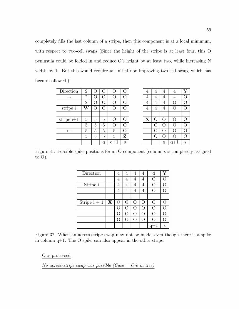
59
completely fills the last column of a stripe, then this component is at a local minimum,
with respect to two-cell swaps (Since the height of the stripe is at least four, this O
peninsula could be folded in and reduce O’s height by at least two, while increasing N
width by 1. But this would require an initial non-improving two-cell swap, which has
been disallowed.).
Direction 2 O O O O 4 4 4 4 Y→ 2 O O O O 4 4 4 4 O
2 O O O O 4 4 4 O Ostripe i W O O O O 4 4 4 O O
stripe i+1 5 5 5 O O X O O O O5 5 5 O O O O O O
← 5 5 5 5 O O O O O5 5 5 5 Z O O O O
q q+1 s q q+1 s
Figure 31: Possible spike positions for an O-component (column s is completely assignedto O).
Direction 4 4 4 4 4 Y4 4 4 4 O O
Stripe i 4 4 4 4 O O4 4 4 4 O O
Stripe i + 1 X O O O O O OO O O O O OO O O O O OO O O O O O
q+1 s
Figure 32: When an across-stripe swap may not be made, even though there is a spikein column q+1. The O spike can also appear in the other stripe.
O is processed
No across-stripe swap was possible (Case = O-b in tree).

60
See figures 31 and 32, as fill proceeds, if W starts as a spike, we will either stop
short of W’s column when assign O’s and W remains a spike, or continue filling with O’s,
past W’s column, and X could possible become a spike. W (X) can only be moved to
a corner by swapping across stripe. Since we know that the 5 (4) component does not
have any cells in stripe i (i+1), this swap will increase 5’s (4’s) height, without reducing
the width (the 5 (4) component is assigned completely to three columns and the far right
column must contain at least two of this components cells OR (see figure 32) O’s spike
falls outside the columns containing N, which would have created a “4” island cell, if 4
and O had been swapped; otherwise an across-stripe swap would have been made).
To move Z (Y) to a corner position would require a 5 (4) to be assigned to column
s. This increases the number of columns component 5 (4) appears in. And since 5 (4)
appears in at least three full columns, the row count of component 5 (4) can’t be reduced.
Therefore, no improvement is possible.
A N-O across-stripe swap (Case = O-c in tree)
(See figures 22 and 23)
N has a side-spike cell in stripe i+1 (i) and O has a side-spike cell in stripe i (i+1).
When these two cells are swapped, the N cell has effectively been slid from side to top
or bottom of the component. After the swap, O will have no spike cells, but rather a
rectangle in stripe i and a rectangle in stripe i+1 (each rectangle is of width at least 2,
by assumption 1). It follows that O is at a local minimum.
Slider Swaps were performed
The O component is the slider component (Case = O-d in case tree)
(see figure 33)
In figure 33, both W and Z are potential O spikes. Since component O is a slider
component, then Z is on the bottom border of the component. In this case, O is the only

61
N N O O O O ODirection N N O O O O O→ N N O O O O O
N W O O O O O
5 5 Z 4 4 45 5 5 4 4 45 5 5 4 4 45 5 5 4 4 4b
Figure 33: A top-slider swap component
component that appears in both stripes. The only corners to which Z could be moved
are all in the upper stripe. But those positions are assigned to components that only
appear in the upper stripe. So any reduction in Z’s height will produce an increase in
height for the swapping component.
For the case of W, we need only look at at components N and 5. The only corner
position that W could be moved into occurs in the bottom stripe. Moving a 5 to the
upper stripe will not decease 5’s width, but will increase 5’s height. Therefore, this type
of swap produces no improvement.
Therefore, this O component is at a local minimum before and after a slider swap.
The argument for the slider cell (Z) being at the top of the component is similar.
TYPE-N COMPONENTS
The cases for showing that N is at a local minimum are listed in the tree as shown in
figure 34. If N is not involved in any type of swap, then N only appears in one stripe, and
only a within-stripe swap could possible improve N. In this case, N could not possibly be
a slider configuration.
The other case occurs if N was involved in some type of swap. If N were involved in
an across-stripe swap with O, then N may or may not be a slider component. If N were
not involved in an across-stripe swap, then N appears only in a single stripe, but could
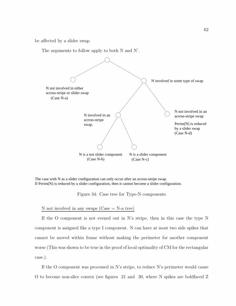
62
be affected by a slider swap.
The arguments to follow apply to both N and N’.
N not involved in eitheracross-stripe or slider swap
(Case N-a)
N involved in some type of swap
N involved in anacross-stripeswap.
N not involved in anacross-stripe swap
(Case N-b)N is a slider component
(Case N-c)
(Case N-d)
N is a not slider component
Perim(N) is reducedby a slider swap
The case with N as a slider configuration can only occur after an across-stripe swap.If Perim(N) is reduced by a slider configuration, then it cannot become a slider configuration.
Figure 34: Case tree for Type-N components
N not involved in any swaps (Case = N-a tree)
If the O component is not evened out in N’s stripe, then in this case the type N
component is assigned like a type I component. N can have at most two side spikes that
cannot be moved within frame without making the perimeter for another component
worse (This was shown to be true in the proof of local optimality of CM for the rectangular
case.).
If the O component was processed in N’s stripe, to reduce N’s perimeter would cause
O to become non-slice convex (see figures 21 and 30, where N spikes are boldfaced Z

63
and 4). Since N occupies more than four columns and only possible spike position is at
the left boundary, the N spike would have to be moved to a corner position, reducing N’s
perimeter by two. In doing so, we would make O non-slice convex, thereby increasing
O’s perimeter.
N involved in a swap
N involved in an across-stripe swap, but is not a slider component. (Case N-b in tree)
The side spike for N has been slid to either the top or bottom of the component. The
N component can now only have one side spike and a slider spike. The bottom spike can
occur in any cell between columns b and e, inclusive, as shown in figure 35 (Otherwise,
the column count for N would increase and no improvement in total perimeter possible.
This could only occur if O’s spike is in a column outside of N’s enclosing frame; and we
said that this swap would not be made.).
I N N N N N OI N N N N N OI N N N N N ON N N N N N O
b N e O
Figure 35: N component after an across-stripe swap
As in the case for the O component, we have shown that the leftside N spike can’t be
moved within frame and that the bottom N spike can’t be moved into the upper stripe
in column b. The only other possible move for the N spike is to column e+1, but there
are no corners in this column.
It follows that N’s component, as the slider component, is at a local minimum after
one or more slider swaps.
N is in an across-stripe swap AND is a slider component. (Case N-c in tree)
The proof is exactly the same as for case N-b. The spikes, at the side or bottom,

64
can’t be moved within the enclosing rectangle without increasing the perimeter for the
other component.
N was subjected to a slider swap only (Case = N-d in tree)
This situation can occur if the neighboring O component in stripe i (i+1) is the slider
component. In this case, N component in stripe i+1 (i) becomes a rectangle and cannot
be improved.
TYPE-I COMPONENTS
Figure 36 is the case tree for proving that I is at a local minimum. From the discussions
for the two previous types of components, we know that I is never involved in an across-
stripe swap (swapping with either the O component or the N component would not
produce an improved total perimeter). Therefore, an I-component can only appear in
one stripe and can never be a slider component. A type-I component can only be involved
in slider swaps as the component whose perimeter is going to be reduced. So we only
have to look at the cases of slider swap or not.
I not involved in aslider swap.
I not involved ina slider swap
(Case I-a) (Case I-b)
Figure 36: Case tree for Type-I components
Fact 3.5 For type I components, only within-stripe swaps offer the possibility of improve-
ment.
I not involved in a slider swap (Case = I-a)

65
Previous Stripe C C C C C C
Direction Y I I C← I I I
I I II I II I ID I I X
D D D D D D
Figure 37: A Type I component
To swap cells with another type I processor will not reduce the perimeter (this was
shown to be true in the proof of local optimality of CM for rectangular grids). A non-
slider I-N swap is analyzed in the same way, and therefore no improvement is possible.
An I-O swap within stripe is impossible, because I and O are not adjacent within the
same stripe..
I involved in a slider swap (Case = I-b)
Case - An I-O/N swap (see figure 37)
I is a rectangle and cannot be further reduced (in fact, any swap will increase I’s
perimeter).
We have now shown that the grid is at a local minimum, by showing that none of the
components can be improved after the second phase of the algorithm.
2
The next algorithm was developed to reduce the effect of peninsulas on the overall
perimeter.
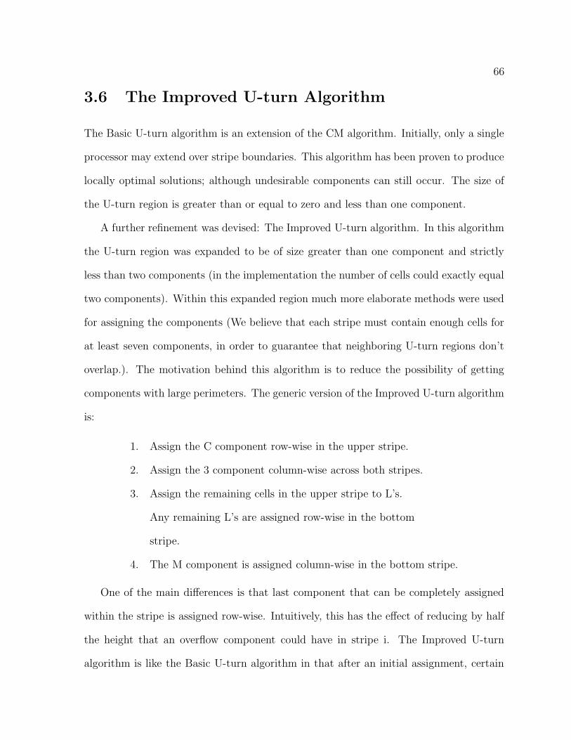
66
3.6 The Improved U-turn Algorithm
The Basic U-turn algorithm is an extension of the CM algorithm. Initially, only a single
processor may extend over stripe boundaries. This algorithm has been proven to produce
locally optimal solutions; although undesirable components can still occur. The size of
the U-turn region is greater than or equal to zero and less than one component.
A further refinement was devised: The Improved U-turn algorithm. In this algorithm
the U-turn region was expanded to be of size greater than one component and strictly
less than two components (in the implementation the number of cells could exactly equal
two components). Within this expanded region much more elaborate methods were used
for assigning the components (We believe that each stripe must contain enough cells for
at least seven components, in order to guarantee that neighboring U-turn regions don’t
overlap.). The motivation behind this algorithm is to reduce the possibility of getting
components with large perimeters. The generic version of the Improved U-turn algorithm
is:
1. Assign the C component row-wise in the upper stripe.
2. Assign the 3 component column-wise across both stripes.
3. Assign the remaining cells in the upper stripe to L’s.
Any remaining L’s are assigned row-wise in the bottom
stripe.
4. The M component is assigned column-wise in the bottom stripe.
One of the main differences is that last component that can be completely assigned
within the stripe is assigned row-wise. Intuitively, this has the effect of reducing by half
the height that an overflow component could have in stripe i. The Improved U-turn
algorithm is like the Basic U-turn algorithm in that after an initial assignment, certain
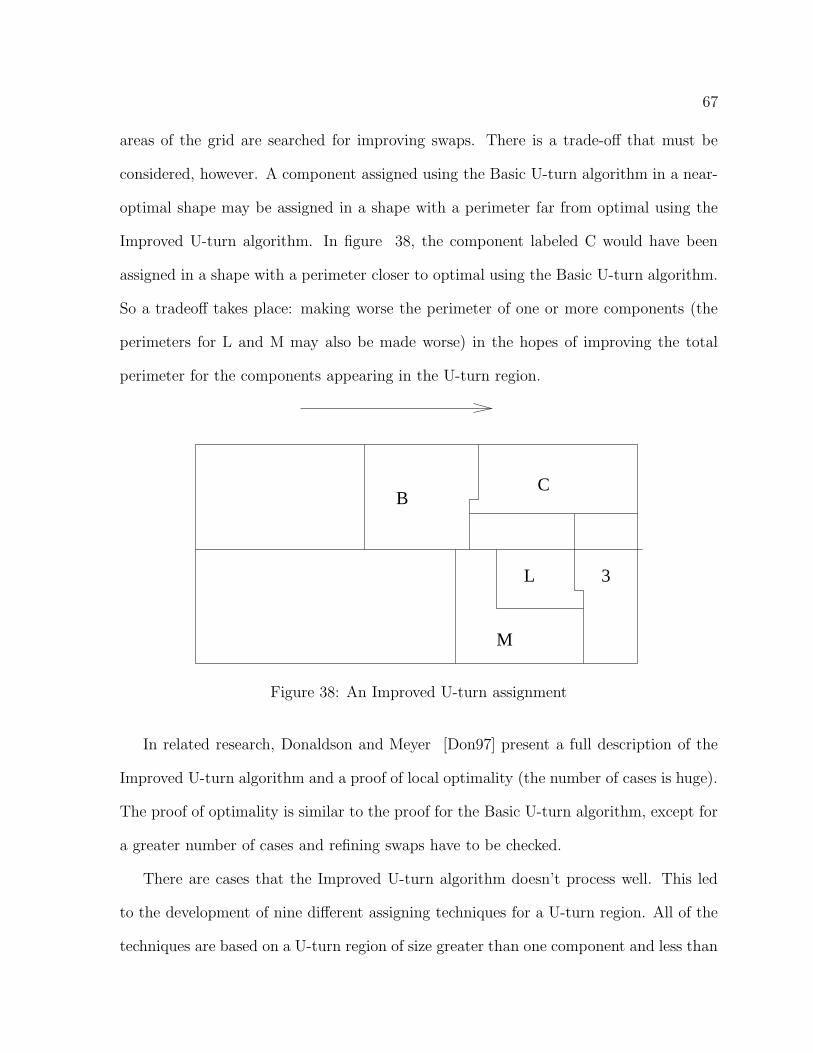
67
areas of the grid are searched for improving swaps. There is a trade-off that must be
considered, however. A component assigned using the Basic U-turn algorithm in a near-
optimal shape may be assigned in a shape with a perimeter far from optimal using the
Improved U-turn algorithm. In figure 38, the component labeled C would have been
assigned in a shape with a perimeter closer to optimal using the Basic U-turn algorithm.
So a tradeoff takes place: making worse the perimeter of one or more components (the
perimeters for L and M may also be made worse) in the hopes of improving the total
perimeter for the components appearing in the U-turn region.
BC
3L
M
Figure 38: An Improved U-turn assignment
In related research, Donaldson and Meyer [Don97] present a full description of the
Improved U-turn algorithm and a proof of local optimality (the number of cases is huge).
The proof of optimality is similar to the proof for the Basic U-turn algorithm, except for
a greater number of cases and refining swaps have to be checked.
There are cases that the Improved U-turn algorithm doesn’t process well. This led
to the development of nine different assigning techniques for a U-turn region. All of the
techniques are based on a U-turn region of size greater than one component and less than
68
two. The actual patterns of assignment are shown in chapter 6.
The theme of all these patterns is to use the best possible assigning pattern for a given
situation. There are cases for which CM does a good job. There are other cases where
column assigning does better. At each U-turn region, all nine assignments processes are
tried and the best perimeter is kept.
There is another more subtle benefit that comes with the identification of a U-turn
region. At the point where the U-turn region starts, an integral number of components
will have been assigned. The perimeters of these completely assigned components are
independent of the assignments for the rest of the grid. This is a key idea that will be
exploited in the next chapter when defining subproblems.
3.7 Unbalanced Partitions
The methodology developed in this chapter is still valid if P does not divide the number
of cells in the grid, |V |. Our arguments were not based on the area per component, but
if there were enough remaining cells within a stripe to to assign a component. If P does
not divide |V |, then (|V | mod P) components will be assigned to ((|V | div P) + 1) cells.
The remaining components will be assigned to (|V | div P) cells. The components can
be assigned in any order, just so long as a record is kept of how many of each type of
component have be assigned.
3.8 Summary
Besides developing algorithms that produce locally optimal solutions, the identification
of the U-turn area was the most important discovery of this section. For most stripes,

69
those components appearing outside of the U-turn region tend to have perimeters that
are close to the optimal perimeter. But bad things happen within the U-turn region. In
the implementation that follows, several different stripe assignment procedures are used
to reduce the chance of occurrence of components with perimeters that deviate greatly
from the lower bound.
The second benefit occurred by careful consideration of the role of the U-turn region.
The U-turn region is basically that part of a stripe that possibly contains a non-integral
number of components. That part of the stripe that precedes the U-turn region plus all
the cells appearing above the stripe can be assigned an integral number of components,
in other words a subproblem. This fact plus the fact that an optimal solution possesses
two traits that are present in problems that dynamic programming is applicable lead to
the discovery of polynomial-time algorithms.

70
Chapter 4
Subproblems for the
Dynamic-Programming Approach
4.1 Introduction
The ability to define a subproblem [DM99] is the foundation upon which the algo-
rithms to be presented are based. The subproblems yield an efficient way of organizing
intermediate results, which in turn eliminates redundant calculations. This reduction
in redundancy allows an expanded set of graphs to be handled (as compared to Martin,
who considered only the case of domains yielding stripes containing an integral number of
components) and finds the optimal set of stripe heights (as compared to Christou-Meyer),
while maintaining a polynomial run-time.
For a given set of stripes, the number of components varies from stripe to stripe.
Within a stripe, after a component has been completely assigned, we know that an
integral number of components have been assigned. This implies that a grid graph can
be partitioned into two parts, each containing an integral number of components, by just
splitting the graph at the last component assigned. Which component should be used
for this division? By assumption, each stripe does contain a final component that is
completely assigned to the stripe. (If this was the last component that could have been
completely assigned within the stripe, then the Basic U-turn algorithm can be used for

71
assigning the cells. If the next to last component was chosen, then the Improved U-turn
Algorithm can be used.) This last component assigned also defines a U-turn region.
In this chapter, three main topics will be discussed. The first is subproblem definition.
The second topic is the relationship between subproblems and stripes. The last point is
that the subproblems possess properties that may be exploited in order to construct a
shortest-path version of the problem and a dynamic-programming solution of the original
problem.
4.2 Terms and Definitions
The following example, figure 39, is presented in order to demonstrate concepts and
definitions that will appear in the paper.
For this grid, there are 360 cells to be assigned among 9 processors. The 26 rows
(numbered 0 to 25) have been partitioned into four stripes. At most one component is
allowed to “overflow” from one stripe into the next stripe. All components are assigned
column-wise, top to bottom. For those components that appear in two stripes, all the
remaining cells in stripe i are assigned first, then the remaining required number of cells
are assigned column-wise in stripe i+1. The total perimeter of this solution is 294. In
chapter 5, figure 52 contains a four-stripe optimal stripe partition of the same graph
which produced a perimeter of 282. The fill procedure used for obtaining this optimal
solution is described in Chapter 6.
Definition - A begin-end row pair defines a stripe as the collection of cells with
corresponding row indices (in figure 39, stripe 1 is defined by the begin-end-row pair
(0,6)).
Definition - A row in a grid is said to be an end-row if it is the last row in a stripe
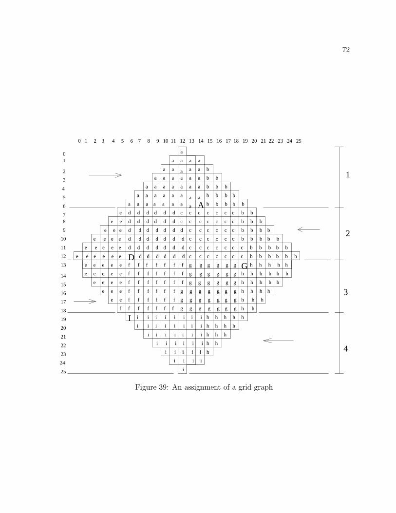
72
12
13
14
11
10
9
87
6
5
01
2
3
4
15
16
17
18
19
20
21
22
23
24
25
0 1 2 3 4 5 6 7 8 9 10 11 12 13 14 15 16 17 18 19 20 21 22 23 24 25
1
2
3
4
a
a
a
a
a
a
a
a
a
a
a a a a a
a
a
a
a
a
a
a
a
aa
a
a
a
a a
a a
a a
a a
a a
a A
b
b b
b b b
b b b b
b b b b b
b b
b b b
b b b b
b b b b b
b b b b b
b b b b b b
c c c c c c
c c c c c c
c c c c c c
c c c c c c
c c c c c c c
c c c c c c c
c
c
d d d d d d
d d d d d d
d d d d d d d
d d d d d d d
d d d d d d d
D d d d d d de e e e e e
e e e e e
e e e e
e e e
e e
e
e
e
e
e
e
e
e
e
e
e
e
e
e
e
e
e
e
e
e
f
f f f f f f f
f f f f f f f
f f f f f f f
f f f f f f
f f f f f f
f f f f f f
g g g g g g Gg g g g g g
g g g g g g
g g g g g g g
g g g g g g g
g g g g g g g
h h h h h
h h h h h h
h h h h h
h h h h
h h h
h h
hh
h
h
h
h
h
h
h
h
h
h
h
h
h
I i i i i i i i i
i i i i i i i i
i i i i i i i
i i i i i i
i i i i i
i i i i
i
Figure 39: An assignment of a grid graph

73
(in figure 39, rows 6, 12, 18, and 25 are end-rows). A begin-row is defined similarly.
Definition - A subset of the grid is said to be filled if all of its cells have been
assigned.
Definition - Within a stripe, a divider cell will be the last cell of the last com-
ponent whose assignment was completed within a stripe (in 39, the uppercase A, D,
G, and I are divider cells). The reader should understand that for the given example,
the divider cells corresponded to the last components that could be assigned within the
stripe. In the implementation, the divider cell was chosen to be the last cell assigned to
the next-to-last component that could be completely assigned within the stripe (under
most circumstances). In the implementation, the divider cell is a data structure that
eliminates the need to keep track of individual cells in in the U-turn region (defined
below).
For stripe i, defined by the begin-end row pair (bi, ei), we assume that a divider cell
position for this stripe is uniquely determined by the fill procedure and the pair (bi, ei),
and is independent of prior stripes. We assume that all cells in stripe i-1 up to and
including the divider cell are assigned before we consider the assignment of cells in stripe
i. This will allow an incrementally discovered partition of the graph.
Definition - A U-turn region for stripe i consists of those cells within stripe i that
“follow” the divider cell and hence are not assigned until stripe i+1 is considered.
In figure 39, the upper regions corresponding to the cells assigned to components b,
e, and h are the U-turn regions.
Definition - Those cells required to complete the assignments for components as-
signed within the U-turn region are called overflow.
Definition - A begin-end-row pair is valid if the corresponding stripe contains a
divider cell.

74
Definition - A set of end-rows (r1, r2, ..., ri) is said to be a feasible sequence of
end-rows if:
for i ≥ 0, (ri+1, ri+1) is a valid stripe (where r0 = -1).
The corresponding sequence of begin-end-row pairs is ((0,r1), (r1+1,r2),..., (ri−1+1,ri))
(note: the use of valid-stripe sequences implies the existence of a divider cell within each
stripe).
The expressions component and configuration will be used interchangeably below.
Although, in the graph literature components are normally considered to connected, we
do not assume this below.
Definition - A subproblem is valid if and only if it can be partitioned by a feasible
sequence of end-rows.
The next definitions applies to the “state graph” constructed in the shortest-path
version of the stripe-height problem.
Definition - A vertex in the state graph is uniquely defined by a begin row, an end
row, and direction of assignment within that stripe in the original grid graph. In the
figures to follow, a vertex is defined by (bi, ei, di). An ordered triple may be a valid
vertex label if and only if bi and ei define a valid stripe.
For the constructions to follow, we further restrict what vertices will be considered.
We only consider vertices that correspond to valid subproblems.
For a given pair of vertices, (B,E,D) and (B’,E’,D’), there is a directed edge connecting
the vertices if and only if D = (D + 1) mod 2 and B’ = E + 1.
In section 4, for the original grid, it will be shown that

75
1) bi, ei, and di uniquely define a subproblem;
2) If there is an edge between (B,E,D) and (B’,E’,D’), then (B’,E’,D’)
is a one-stripe extension of the subproblem defined by (B,E,D); and
3) The cells contained within this one-stripe extension are uniquely defined
by (B,E,D) and (B’E’,D’).
Definition - Define perim (bi−1,bi,ei,di) to be the perimeter for the cells falling within
the stripe defined by the extension of (bi−1,ei−1,di−1) to (bi,ei,di−1+1 mod 2), where bi =
ei−1 + 1.
4.3 Defining Subproblems
4.3.1 Identifying Subproblems
In this section, a method for breaking up the original problem into similar but smaller
subproblems will be presented. This is a the key step in the dynamic-programming
and greedy algorithms that will be presented later in this dissertation.
Definition - Given a grid G that contains M rows. Let bi and ei be two row indices
within G such that bi ≤ ei. Let di be the direction of assignment within this stripe. And
let ci be a divider cell appearing within this stripe. We say that bi, ei, and di define a
subproblem.
In the following example, we assume that an integral number of components can be
assigned to the cells in the union of regions A and B, where ci denotes the divider cell in
stripe i.
If the graph is symmetric, then bi and ei uniquely define a subproblem. If the grid is
not symmetric, then direction of assignment becomes a factor.
For the two configurations appearing in figure 41, the assignments for the last stripes

76
A
b_i
e_i
Original Problem Subproblem
A
B B
c_i
Figure 40: Subproblem example
are in opposite directions. Both subproblems are defined by the same pair of rows, but
the configurations (U and U’) of remaining unassigned cells are different. Again, this
difference may result in different perimeter increases when the next stripe is added.
U U’b_i
e_i
c_i c_i’
Figure 41: Direction of assignment affects the configuration of remaining cells.
For the discussion to follow, we assume that each stripe contains a divider
cell and focus on the role of the divider cell within a stripe.

77
4.3.2 Selecting a Divider Cell
For the arguments to follow, the choice of divider cell ck for a given stripe (bk,ek,dk) must
be independent of the height of the previous stripe. Also, for a given striping assignment,
once a divider cell has been identified, the configuration of unassigned cells that appear
within the given stripe (U-turn region) must be independent of the height of the previous
stripe. Any assignment of components to the cells of the stripe may be used provided
that the U-turn region is independent of the previous stripe and all unassigned cells are
in the current stripe (and none are in the previous stripe).
For the algorithms to follow, we choose ci to be the last cell in the last component
assigned (assuming all the cells in the previous stripe have been assigned and a column-
wise assignment was used for the last components) before the U-turn region for stripe
(bi,ei,di).
For a given fill procedure, a begin-end-row pair and the direction of assignment
uniquely define a subproblem (by default, also uniquely defined are the U-turn region
for the current stripe and the remaining cells that will have to be assigned). In partic-
ular, these three variables uniquely define the last cell of a subproblem. Assuming that
the subproblem is valid, then figure 42 shows how a begin-row, end-row, and direction
of assignment determine a subproblem, independent of how previous subproblems have
been defined.
For our choice of ci, we are guaranteed that all of the cells above stripe (bi,ei,di) will
have been assigned before any cells in this stripe are assigned. In figure 42 the number
of cells above row bi is independent of the choice for bi−1, assuming that there exists valid
subproblem defined by (bi−1,bi-1,di + 1 mod 2). It then follows that the U-turn region
within the stripe defined by stripe (bi,ei,di) is independent of the previous stripe.

78
Last cell assigned for both configuration is the same.
Number of cells in these areas are equal.
b_i
e_i
b_i-1b_i-1’
No. of cells = T - a’
No. of cells = a’No. of cells = a
No. of cells = T - a
Figure 42: Begin-row end-row and direction uniquely determine a subproblem.

79
Subproblems: Perimeters:No. bi ei di U-turn Current Total Subproblem
region(Ui) stripe(Si/Ui) Increment Perimeter1 0 6 1 0 32 32 322 7 12 0 44 54 98 1303 13 18 1 34 56 90 2204 19 25 0 42 32 74 294
Table 4: Dynamic-programming data for partition in figure 39
This deterministic way of uniquely defining subproblems allows for the use of dynamic-
programming techniques for organizing subproblem results and eliminates redundant cal-
culations (e.g. the subproblem defined by (bi, ei, di), and implicitly ci, may be contained
within several other larger subproblems). This ability to define subproblems also pro-
vides a useful way of identifying vertices and calculating edge weights in the corresponding
shortest-path problem (see Chapter 5,“Description of a State Graph”).
Consider the partitioned grid in figure 39. Examples of the two ways that the
subproblem data can be presented are shown in table 4 and figure 43. Table 4 contains
the perimeter data as organized by the dynamic-programming implementation. Figure
43 presents the data in the form of a weighted graph, with vertices corresponding to
subproblems and edge weights equal to the perimeters for the incremental stripes.
The perimeter for the partition in figure 39 equals 294 (this is the final subproblem
perimeter in the far right-hand column in table 4). This is not an optimal partition.
An optimal stripe-based partition, with perimeter equal to 282, is shown in Chapter 5,
figure 52.
Unassigned Grid
Assigned Grid
(0,6,0) (7,12,1) (13,18,0) (12,25,1)
32 98 90 74 0
Figure 43: Path Data for table 4

80
4.4 Relationship between Subproblems and Stripes
A stripe is defined by a begin-end row pair and direction of assignment. After an as-
signment is made, there will be components completely assigned within the stripe plus
possibly fractional parts of other components at both ends of the stripe (these compo-
nents are assigned to cells appearing in more than one stripe). For this discussion, there
can be at most two partial components appearing within the stripe. In particular, for
stripe i, these partial components would correspond to the overflow from stripe i-1 and
the component assigned partially within the U-turn region for stripe i.
As was stated earlier, (bi−1,ei−1,di−1) uniquely defines a subproblem. These three
quantities also define the U-turn region appearing within stripe i-1. By the same reason-
ing, (bi,ei,di) determines the U-turn region for stripe i. We now have a mechanism for
defining the cells to be included within an “appending” (partial) stripe: those cells that
would have to be appended to subproblem (bi−1,ei−1,di−1) in order to get subproblem
(bi,ei,di) (note: the cells in the U-turn region for stripe i are not included).
Those cells appearing within this “appending” stripe may be assigned independently
of all other cells. This follows from the fact that we have identified a group of cells that
an integral number of processors can be assigned and that the number of cells defined by
the subproblem (bi−1,ei−1,di−1) also allows for an integral number of components to be
assigned.
A feasible solution of the problem can then be thought of as a sequence of “appending”
stripes.

81
b_i-1
e_i-1
e_iStripe i
(b_i,e_i,d_i)
(b_i-1,e_i-1,d_i-1)
Figure 44: Two subproblems defining a stripe.
4.4.1 Construction of a Stripe-based Solution
Perimeter is computed in our approach incrementally, stripe-by-stripe as follows (see
figure 45): perimeter (in the first stripe (0,e1,d1) - U1) is computed, then the perimeter
for (b2,e2,d2) + U1 - U2, is added, etc. Figure 45 shows a fourth iteration of this process.
4.5 Properties of Subproblems
4.5.1 The Existence of Common Subproblems
Figure 46 shows two different sequences of stripe-heights used to partition the given grid.
Both cases contain the subproblem ending with the stripe (b5,e5,d5).
When the same subproblem appears in several other larger problems, the overall
problem is said to possess the property of common subproblems. With respect to the
graph viewpoint, a subproblem is a node and this node appears in multiple paths.

82
b_3
b_4
e_4
U_3U_3
1
2
3
4
1
2
3
4
Figure 45: Incrementally processing a grid

83
1
2
3
4
5
1
2
3
4
5
1
2
3
4
5b_i
e_i
e_i
e_i+1’
6’ 6
Solution 1 Solution 2
Figure 46: Feasible solutions with the same subproblem (stripes 1-5).

84
4.5.2 Optimal Substructure within a Solution
Cormen, Leiserson, and Rivest [CLR90] state that a problem exhibits “optimal” sub-
structure if an optimal solution contains the optimal solutions for the corresponding
subproblems.
e_1
e_2
.
e_t
Optimal
Partition
Optimal partitionfor the subproblemdefined by rows
.
.
.
e_i
e_i-1
(e_i-1 + 1,e_i,d_i)
e_i-2
Figure 47: Optimal Substructure
Given a grid, assume that the sequence of end-rows (e1,e2, ... et−1, et) produces an
optimal solution. Now look at the subproblem ending at stripe (bi,ei,di) (see figure 47).
For this subproblem, if the subsequence (e1,e2, ... ei−1, ei) of the original sequence didn’t
produce an optimal solution within the corresponding subproblem, assuming that the
last stripe was (bi,ei,di)), then the optimal solution for this subproblem could be

85
substituted into the larger solution. This new sequence would produce a better overall
solution, which would contradict the fact that we previously had an optimal solution.
From a graph viewpoint, the shortest path has the property that each sub-path (beginning
at the the start node) is also a shortest path.
4.6 Grid Partitioning as a Shortest-Path Problem
Constructing a sequence of end-rows that partitions a grid is equivalent to determining
reachability from a source to a sink by a certain path within a graph. For a given sequence
of end-rows (0, r1, r2, ... ,rn), we know for any consecutive end-rows, ri, ri+1, that ri+1
is reachable from ri if and only if the begin-end-row pair (ri + 1, ri+1) is a valid stripe.
For the previous methods, the state graph for a particular grid has |V| equal to
the number of valid end-row sequences for lengths 1 to M. Two vertices would have a
connecting edge if and only if for vertices (0, r1, r2, ... ,ri) and (0, r1, r2, ... ,ri, ri+1)
(ri + 1, ri+1) is a valid stripe.
Figure 48 contains a portion of a graph constructed using a naive approach.
In the next chapter, it will be proved that under very limited assumptions that the
number of vertices in this graph is super-polynomial. What the Donaldson-Meyer (DM)
method does is to eliminate certain redundant vertices in the state graph.
Figure 49 contains a graph for the same original grid graph, except that this graph
was constructed using the DM algorithm. In figure 48, there are three paths for which the
corresponding end-row sequences share final subsequences. What DM does is to collapse
down those common parts of the graph. As will be shown in the next chapter, the graph
for DM will have a polynomial number of vertices.

86
(0) (0,r1) (0,r1,r2) (0,r1,r2,r3) (0,r1,r2,r3,r4) (0,r1,r2,r3,r4,r5)
(0.r1,r2,r3,r4,r5)
(0,r1,r2,r3,r4,r5,r6)
(0) (0,s1) (0,s1,s2) (0,s1,s2,s3) (0,s1,s2,s3,s4,s5)
(0,s1,s2,s3,s4)
(0) (0,t1) (0,t1,t2) (0,t1,t2,t3) (0.t1.t2.t3.t4) (0,t1,t2,t3,t4,t5,t6)
(0,t1,t2,t3,t4,t5)
t3 = s2 = r4
t4 = s3 = r5
t5 = s4 = r6
t6 = s5 = r7
Figure 48: A naive state-graph construction.
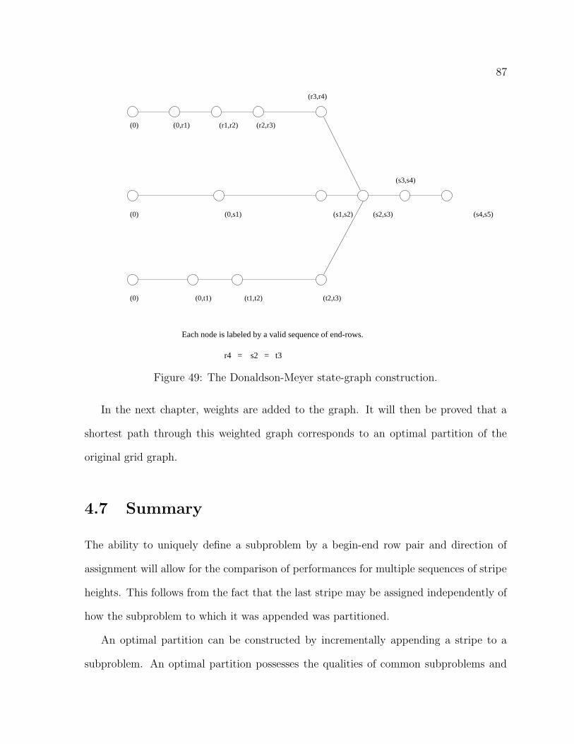
87
Each node is labeled by a valid sequence of end-rows.
(0) (0,r1) (r1,r2) (r2,r3)
(r3,r4)
(s3,s4)
(0) (0,s1) (s1,s2) (s2,s3) (s4,s5)
(0) (0,t1) (t1,t2) (t2,t3)
r4 = s2 = t3
Figure 49: The Donaldson-Meyer state-graph construction.
In the next chapter, weights are added to the graph. It will then be proved that a
shortest path through this weighted graph corresponds to an optimal partition of the
original grid graph.
4.7 Summary
The ability to uniquely define a subproblem by a begin-end row pair and direction of
assignment will allow for the comparison of performances for multiple sequences of stripe
heights. This follows from the fact that the last stripe may be assigned independently of
how the subproblem to which it was appended was partitioned.
An optimal partition can be constructed by incrementally appending a stripe to a
subproblem. An optimal partition possesses the qualities of common subproblems and

88
optimal substructure.
The qualities of common subproblems and optimal substructure must be present for
dynamic programming to be applicable ( [CLR90], p.309). In chapter 5, both a dynamic-
programming algorithm and a greedy algorithm will be presented for identifying the
sequence of stripe heights that produce an optimal partition. (The methods only differ
in how the data for subproblems are organized.)
The Donaldson-Meyer approach for organizing the results for subproblems eliminates
redundant calculations. Figure 50 shows what happens when constructing a state graph
when the property of common subproblem is not used.
(e_i, e_2, ..., e_i) (e_1, e_2, ..., e_i, e_i+1)
(e_i, e_2, ..., e_i) (e_1, e_2, ..., e_i, e_i+1’)
Figure 50: An example of redundant states (calculations)
To not use the common subproblem property is fatal when trying to determine the
optimal sequence of stripe heights in polynomial time. In Chapter 5 it will be shown
that the number of feasible stripe-height sequences is super-polynomial.

89
Chapter 5
Optimal Partitioning Algorithms
5.1 Introduction
From the previous section, we know that an optimal solution for a given stripe assign-
ment possesses the properties of common subproblem and optimal substructure. Using
these two properties, both a greedy algorithm and a dynamic-programming algorithm
for obtaining a best stripe-based solution are presented.
The greedy algorithm is actually Dijkstra’s algorithm applied to a transformed graph.
It will be shown that the shortest path in this graph corresponds to an optimal solution
in the original problem.
The dynamic-programming approach was the procedure used to solve the problem.
The dynamic-programming recurrence models the action of stripping off the last stripe
and solving a smaller, but similar, problem.
These two approaches only differ in how the solution is constructed. The greedy
algorithm works bottom-up. At each step, the best new stripe is added. Eventually, all
stripes containing the last row in the original grid will be considered, thus solving the
problem.
The dynamic-programming algorithm works top-down, but the implementation ac-
tually is bottom-up. The dynamic-programming approach looks at all the possible final
90
stripes and associated subproblems and selects the pair that produces an optimal solu-
tion, after recursively solving all the subproblems.
For the remainder of the chapter, it will be shown that an “brute-force” exhaustive
search of feasible solutions is not practical. Then both the shortest-path and dynamic-
programming approaches will be analyzed.
5.2 Stripe-Height Selection
In the earlier work of Martin [Mar98] and Christou-Meyer [CM96], selection of stripe
heights was the critical factor in determining the best solution possible when using a
stripe-based algorithm.
Given a rectangular grid, Martin [Mar98] converts the original problem into a knap-
sack problem and uses knapsack software [MT90] for solving the reformulated problem.
This algorithm will produce the best stripe-based solution, under the following assump-
tions. In addition to the rectangular grid assumption Martin [Mar98] assumes that
there exists a stripe partition in which each stripe contains exactly an integral num-
ber of components. Martin [Mar98] also assumes that MN/P is an integer and that
a column-wise assignment procedure is used. Under these constraints, the perimeter in
each stripe is independent of the perimeter in any other stripe, and the perimeter of a
stripe is independent of position within the grid.
Therefore, for a stripe of a given stripe height, there will be a unique perimeter
associated with that height. The problem can then be thought of as the selection of
a set of heights totaling to M with minimum total perimeter. With respect to the
knapsack problem, the heights correspond to the weights and the perimeters correspond
to the objective values of the associated weights. Optimal solutions of the knapsack
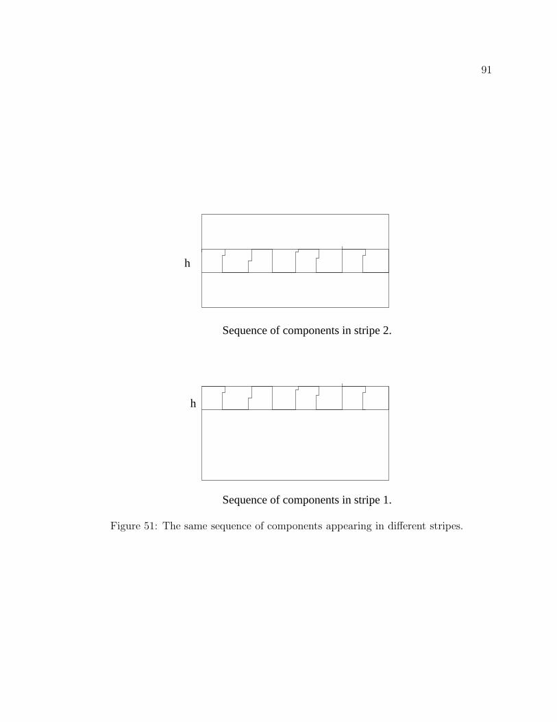
91
h
h
Sequence of components in stripe 2.
Sequence of components in stripe 1.
Figure 51: The same sequence of components appearing in different stripes.

92
problem correspond to optimal stripe partitions (assuming column-wise assignment and
independent stripes).
For CM, the authors relax many of the restrictions (integral number of components per
stripe and rectangular grids). CM doesn’t in general produce optimal stripe partitions,
but does generate high-quality partitions through the use of genetic-algorithm techniques.
The running time for CM can be made to be polynomial. The number of different
feasible solutions that are tried can be limited to guarantee a polynomial running time.
Since Martin [Mar98] only considered rectangular domains, M, N, and P are all that
are required for describing the graph. The length of the input is then O(ln M + ln N
+ ln P). Because Martin restricts the class of inputs to the Knapsack problems that he
studied, it is not known if the resulting problem class is NP-Hard.
Whereas the type of problem that Martin [Mar98] studied could be represented with
three numbers, it is assumed that a full adjacency matrix or adjacency list is required
to represent a general grid graph. This assumption guarantees that that the length of
input is bounded below by (V + E). Since E is O(V), we have that the length of input
Ω(V) = Ω(number of cells in the grid).
That raises the question of whether or not it is possible, in a reasonable amount of
time (i.e. polynomial time), to evaluate the perimeter for all the different stripe-height
sequences? In this and later sections, it is assumed that the stripes will run perpendicular
to the major axis of the grid. By making this assumption, bounds are then expressed in
terms of the size of the original problem. Also, a result from [CM96] is needed.
The Christou-Meyer algorithm [CM96] uses the notion of base heights. The base
height, k, for a given grid is equal to the floor of the square root of the area to be assigned
to a processor. For this discussion, we will make the following assumptions:

93
1. The number of rows in the grid, M, is greater than (k+1)2.
2. k ≥ 2.
3. Stripes are perpendicular to the major axis of the grid.
4. Any set of consecutive k-1 rows contains at least one divider cell.
The first assumption is stronger than what Christou-Meyer [CM96] needed. This
stronger assumption was made so that a certain inequality in the proof that follows
would be easier to manipulate. Christou-Meyer [CM96] only assumed that M ≥ k(k-1).
The second assumption is required to guarantee a valid range of stripe heights in the
proof. The third assumption is needed to bound the cells in the grid by a function of
M. The fourth assumption is required so that we are only counting realistic stripes. This
says that there will always be enough cells within stripe i+1 to assign any overflow from
stripe i. This guarantees that components will only appear in at most two stripes, which
is in keeping with the spirit of the striping algorithm.
If we define the number of rows in the grid to be M and the base height for each
stripe to be k with the above assumptions, [CM96] showed that there exist non-negative
integers α and β st.
M = α(k) + β(k+1)
This sequence of α k’s and β (k+1)’s will now be called a base feasible solution.
In order to discover a lower bound on the total number of valid stripe-height sequences,
we need only consider sequences for which every stripe height falls within the following
range:
[ k-1, k, k+1, k+2].
With these assumptions, we now have the following theorem:

94
Theorem 5.1 The number of feasible solutions is Ω (3M0.5/4).
Proof
In order to prove this result, we will only look at those feasible solutions that contain
S = α + β stripes. There could be feasible solutions that use a different number of
stripes, but these solutions will only add to the overall count, and would only increase
the lower bound.
Assume that α > β (if β > α a similar argument with β replacing α can be given).
The stripes associated with α are of height k. Let’s further divide the α stripes into two
approximately equal groups, so that the smallest group is of size at least α/2 - 1. Call
this group of stripes the independent stripes. The remaining α stripes along with all
the β stripes will be called the dependent stripes.
For any stripe within the set of independent stripes, the height may increased/decreased
by one or may remain the same, with respect to the base height, provided the opposite
change is made to the corresponding dependent stripe. If the heights for the remaining
β stripes are held constant, then we have that there are at least
3α/2/3 ≥ 3S/4/3 ≥ 3M/(k+1)4/3 ≥ 3M0.5/4/3
The second inequality follows from the fact that we have:
M = α(k) + β(k+1)
M/(k+1) = α(k)/(k+1) + β(k+1)/(k+1)
= α(k)/(k+1) + β
≤ S
The third inequality follows from the assumption that M ≥ (k+1)2
2

95
To convert this bound into the units of the input. If M equals the height of the major
axis of the rectangle that encloses the grid, we have that
M ≤ (number of cells in grid) ≤ M 2
If the grid were a single row of cells, then M would equal the number of cells. If
the grid were a square, then the number of cells equals M 2. Regardless, the number of
stripes is super polynomial with respect to the number of cells in the grid.
3M0.5/4/3 ≥ 3(no.ofcells)0.25/4/3
From this result, we know that there are at least an super polynomial number of
feasible solutions and that an exhaustive search it is not practical.
On page 71 of [Chr96] a bound on the total number of ways that the rows of a grid
can be partitioned is calculated. What Christou [Chr96] counts and what is counted in
theorem 5.1 of this dissertation are not the same thing. Included in Christou’s result are
non-feasible partitions, with respect to striping.
In [Chr96], given M rows, the 2M−1 figure contains stripes that may not contain
enough cells to assign one processor. That means that a component could appear in
three “stripes”. It is not clear to the author if these are stripes that really should be
considered. Theorem 5.1 discriminates as to what stripes may be considered and alters
the count accordingly.
5.3 A Detailed Example
The following example will be used to demonstrate both the the shortest-path approach
and the dynamic-programming approach. For the sake of constructing an example, we

96
consider only a small number of possible stripe heights. The results presented here
were generated using an implementation that differed slightly from the the algorithms to
be presented. A more sophisticated approach was taken to handle U-turn regions (see
Chapter 6) . Restricting the total number of stripe heights also makes presenting the
shortest-path problem on one page feasible.
In chapter 4, a diamond shaped grid (see figure 39) was presented, but was not
partitioned optimally. The partition in figure 52 is thought to be fairly close to the
optimal partition based on striping.
The only possible improvement would come from expanding the set of valid stripe
heights (Later, all valid stripes were considered. The perimeter for the partition in
figure 52 is optimal, with respect to the given fill procedure. It is also easy to see that
it is locally optimal. However, it is not globally optimal, since the order in the central
column of 1’s and 2’s may be interchanged to improve the total perimeter. This illustrates
the potential for even more sophisticated fill procedures.). Increasing the number of stripe
heights can be done, but this introduces the possibility of violating assumptions about
the number of components within a stripe. More will be said about this in Chapter 6.
In the sections to follow, it is assumed that:
1. Every stripe contains at least one divider cell.
2. For the chosen stripe assignment, the U-turn region for a given stripe is independent
of the height of the previous stripe.

97
6 6 6 6 6 6 5 5 5 5 5 5 5 4 4 4 4 4 4 3 3 3 3 3 3 36 6 6 6 6 5 5 5 5 5 5 5 4 4 4 4 4 4 3 3 3 3 3 3
6 6 6 6 5 5 5 5 5 5 5 4 4 4 4 4 3 3 3 3 3 36 6 6 5 5 5 5 5 5 4 4 4 4 4 4 3 3 3 3 3
6 6 6 6 6 5 5 5 5 5 5 5 4 4 4 4 4 4 3 3 3 3 3 36 6 6 6 6 6 5 5 5 5 5 5 4 4 4 4 4 4 3 3 3 3 3 3
6 6 6 6 6 7 7 7 7 7 7 7 7 8 8 8 8 8 8 8 8 86 6 6 7 7 7 7 7 7 7 7 8 8 8 8 8 8 8 8 8
6 6 7 7 7 7 7 7 7 7 8 8 8 8 8 8 8 86 7 7 7 7 7 7 7 7 8 8 8 8 8 8 8
7 7 7 7 7 7 7 7 8 8 8 8 8 89 9 9 9 9 9 9 9 9 9 9 8
9 9 9 9 9 9 9 9 9 99 9 9 9 9 9 9 9
9 9 9 9 9 99 9 9 9
9
1 1 1 1 1 1 1 1 2 4 4 4 4 4 3 3 3 31 1 1 1 1 1 1 2 2 2 2 2 2 2 2 2
1 1 1 1 1 1 2 2 2 2 2 2 2 21 1 1 1 1 2 2 2 2 2 2 2
1 1 1 1 2 2 2 2 2 21 1 1 1 2 2 2 2
1 1 1 2 2 21 1 2 2
1
Figure 52: An optimal partition for a given set of stripe heights

98
(0,8,0)
(0,8,1)
0,9,0)
(0,9,1)
(0,10,0)
(0,10,1)
(9,14,1)
(9,14,0)
(10,14,0)
(10,14,1)
(15,18,0)
(15,18,1)
(15,19,0)
(15,19,1)
(19,25,0)
(19,25,1)
(20,25,0)
(20,25,1)
(11,19,0) (11,19,1)
Unassigned
Grid
Assigned
Grid
Figure 53: Partial state-graph

99
Subproblem Data Previous SubproblemStripe Total
bi ei di Perim Perim bi−1 ei−1
0 8 0 34 34 0 00 8 1 36 36 0 00 9 0 36 36 0 00 9 1 36 36 0 00 10 0 68 68 0 00 10 1 68 68 0 09 14 0 118 154 0 89 14 1 120 154 0 810 14 0 124 160 0 910 14 1 124 160 0 911 19 0 124 192 0 1011 19 1 124 192 0 1015 18 0 34 188 9 1415 18 1 34 188 9 1415 19 0 34 188 9 1415 19 1 34 188 9 1419 25 0 98 286 15 1819 25 1 98 286 15 1820 25 0 94 282 15 1920 25 1 94 282 15 19
Table 5: Subset of perimeter data for stripe partitioning the grid in figure 52
5.4 A State-Graph Representation of Grid Graph
Partitioning
5.4.1 Background
An optimal partition of a grid graph can be thought of as a sequence of valid stripes, where
each stripe is added incrementally. After each stripe is added, a new valid subproblem
is generated. The discovery of an optimal solution can be thought of as going from the
initial unassigned state to the final fully assigned state in an optimal fashion.
Figure 53 contains the state graph for the data in table 5.

100
If an optimal solution for a (sub)problem is represented by the sequence of stripe-
defining end-rows (r1, r2, ...,rn), the previous theorem showed that the number of states is
super polynomial. To define an optimal solution, are all elements in an end-row sequence
needed? No.
In chapter 4, it was shown that a begin-end-row pair and direction of assignment
define a subproblem. With the sequence (r1, r2, ...,rn) a lot of redundant information is
carried along. The length of the sequence determines the direction of assignment. Instead
of carrying along all the elements of the sequence, all that is really required is a pointer
to the subproblem that the last stripe was appended to. When this is done, the size of
the state graph becomes polynomial.
Figure 53 contains the state graph for the data contained in table 5 (this is the
stripe information for the diamond). When the grid graph is completely unassigned, the
graph is in the state corresponding to the source node, titled “unassigned grid”. The
source node is connected to all nodes that correspond to a valid stripe height. Each of
these nodes is connected to nodes whose corresponding subproblems are just the original
problem plus a valid stripe extension. Because the graph is finite, eventually the node
corresponding to the entire grid graph will be found. The path containing the cross-
hatched edges corresponds to an optimal partition of the original grid graph.
For the remainder of this section, the transformation from the original grid graph to
the state graph will be presented. It must be shown that for this state graph, a directed
and weighted graph, the shortest path corresponds to an optimal partition of the original
graph.

101
5.4.2 Description of a State Graph
For a state graph, the number of vertices equals the total number of valid subproblems.
An edge connects two vertices vi and vi+1 if and only if a valid stripe can be appended
to the subproblem defined by vi to get the subproblem defined by vi+1.
Each node in the graph represents a unique subproblem. From the discussion on
defining subproblems, three variables are required to determine a vertex. Let the ordered
triple (bi, ei, dik) represent a given subproblem(vertex). At most, there are M different
choices for bi. Once bi has been determined, the total number of valid stripe heights (call
this number h, where h ≤ M, and the range of the valid stripe heights is from 1 to h) is
an upper bound on the number of different possible values that ei may assume. For any
given stripe, there are only two directions that an assignment may be made. We get the
following:
total number of vertices(subproblems) ≤ 2Mh
The inequality comes from the fact that under certain circumstances not all M rows
may be beginning rows and not all begin-end-row pairs, (bi, bi+k), k = 0,..,h-1, represent a
valid subproblem. These situations can occur for irregularly shaped objects that contain
blocks of rows that don’t contain enough cells to satisfy all the assumptions. In the
shortest-path problem, there will be two additional vertices: a “source” (unassigned
grid) and a “sink” (assigned grid).
For a given subproblem, an upper bound on the number of different stripes that may
be appended to that subproblem equals the total number of valid stripe heights, h. It
follows that:
total number of edges ≤ the total number of vertices * h
≤ 2Mh2
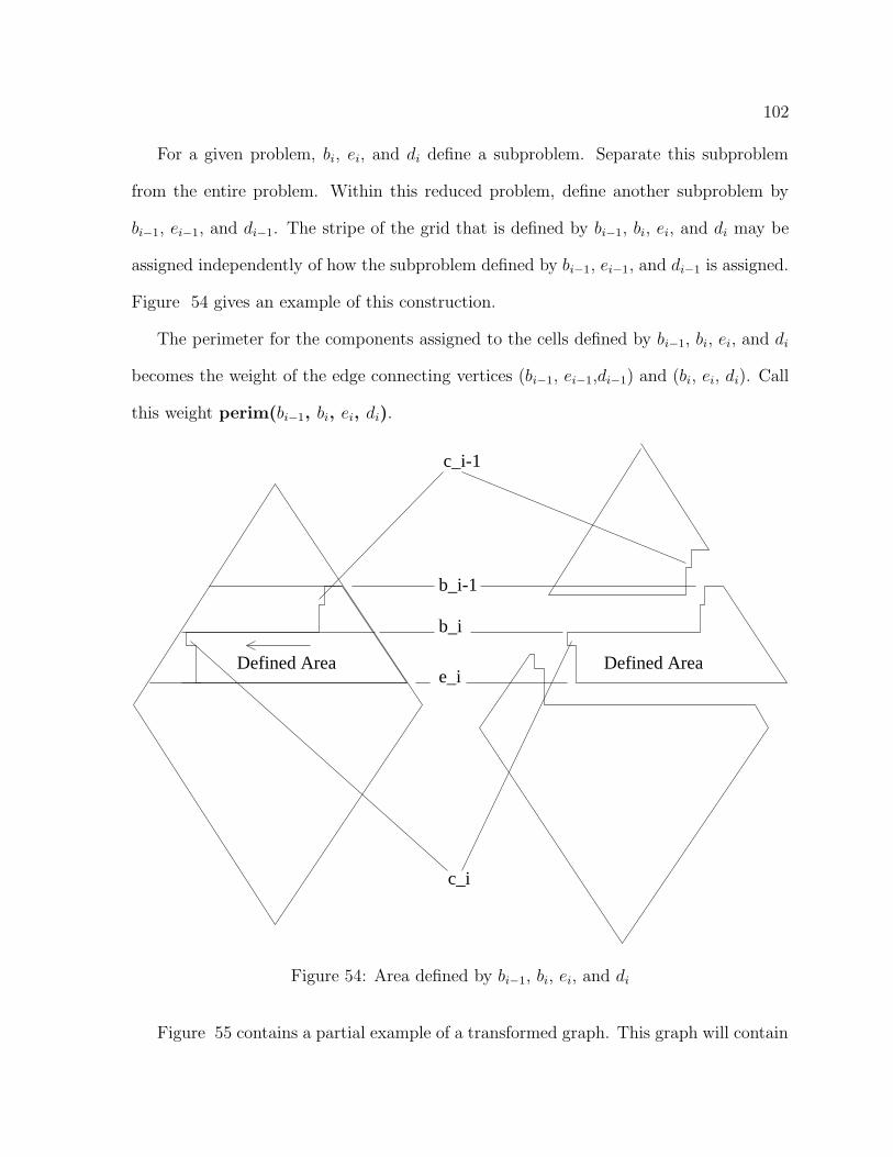
102
For a given problem, bi, ei, and di define a subproblem. Separate this subproblem
from the entire problem. Within this reduced problem, define another subproblem by
bi−1, ei−1, and di−1. The stripe of the grid that is defined by bi−1, bi, ei, and di may be
assigned independently of how the subproblem defined by bi−1, ei−1, and di−1 is assigned.
Figure 54 gives an example of this construction.
The perimeter for the components assigned to the cells defined by bi−1, bi, ei, and di
becomes the weight of the edge connecting vertices (bi−1, ei−1,di−1) and (bi, ei, di). Call
this weight perim(bi−1, bi, ei, di).
c_i
c_i-1
b_i
e_i
b_i-1
Defined AreaDefined Area
Figure 54: Area defined by bi−1, bi, ei, and di
Figure 55 contains a partial example of a transformed graph. This graph will contain

103
one source node (corresponding to an unassigned grid graph), one sink node (correspond-
ing to an assigned grid graph) and a node for each valid subproblem. For the proofs in
this dissertation, it was assumed that the initial stripe always had to be assigned left to
right. For the results in table 5, the first stripe was assigned in both directions. The
one-direction assumption is made to reduce the complexity of the proofs.
0
0
0
0
(*,M,*)
(*,M,*)
(*,M,*)
(*,M,*)Perim(*,*,M,*)
Perim(*,*,M,*)
Perim(*,*,M,*)
Perim(*,*,M,*)
Perim(0,0,h_n,0)
Perim(0,0,h1,0)
Perim(0,0,h2,0)
Perim(0,0,h_n-1,0)
(0,h1,0)
First Stripe Final Stripe
(o,h2,0)
(0,h_n,0)
(0,h_n-1,0)
Intermediate
Stripes
UnassignedGrid
Assigned Grid
Figure 55: Transformed shortest-path graph.
5.4.3 Proof of Optimality
We must now show that the path corresponding to an optimal striping is contained within
the graph.

104
Theorem 5.2 The previously defined graph contains a path corresponding to every fea-
sible sequence of end-rows. Conversely, every path beginning at node 0 corresponds to a
feasible sequence of end-rows.
Proof - (by induction)
Base Case - A sequence of length one. Given that (E) is a feasible sequence, (0,E) is
a valid stripe. It follows that vertex (0,E,0) and the corresponding edge (source vertex)-
(0,E,0) exists within the graph.
Induction Hypothesis - Given a sequence of end-rows of length n, there exists a path
in the graph from the unassigned grid node to the node corresponding to the last stripe
in the sequence.
Induction Step - Given a sequence of n+1 valid stripes, by the induction hypothesis,
there exists a path from the unassigned grid node to the node corresponding to the nth
stripe. Since all the n+1 stripe heights are valid, there must be an edge from the node
corresponding to the nth stripe to the node corresponding to the last stripe.
The converse follows directly from the way the shortest path problem was constructed.
2
Lemma 5.1 The shortest path in the transformed graph corresponds to an optimal stripe-
based solution.
Proof (by contradiction) - From theorem 5.2 , we know that transformed graph
contains the path for an optimal solution. The value of the perimeter for the optimal
striping must equal the shortest path in the graph. For if this were not the case, then
the stripe heights corresponding to the shorter path would produce a better solution in
the original grid graph, which would be a contradiction.
2

105
5.5 A Dynamic-Programming Approach
5.5.1 Background
In Chapter 4 it was shown that an optimal stripe-based partition of a grid graph possessed
two qualities: optimal substructure and common subproblems. These are two properties
that are present when dynamic programming is applicable. For the remainder of this this
section, an optimal solution will be dissected to provide intuition as to why a recurrence
can model the optimal stripe-based solution.
Table 5 contains the striping information for an optimal solution for a given small set
of stripe heights and a stripe assignment process. There are four different ways that the
last stripe may be assigned. The optimal solution is a minimum of these four different
outcomes. An optimal solution is:
optimal solution = perimeter of last stripe in an optimal solution
+ perimeter for corresponding subproblem (last stripe
removed)
Perim(20, 25, 1) = 94 + Perim(15,19,0)
Notice that the value of Perim(15,19,0) must also be optimal, or else the optimal
solution could be substituted, and this would be a better total perimeter than Perim(20,
25, 1), which is a contradiction.
Although the shape of the configuration corresponding to the subproblem defined by
Perim(15,19,0) is no longer a diamond, the same techniques may still be applied. Again,
all the different final-stripe-and-corresponding-subproblem pairs are considered, and the
perimeter for the final stripe-corresponding subproblem pair that produces the best total
perimeter is the value of Perim(15,19,0). It was this observation that lead to the discovery
of the recurrence to be presented.

106
The remainder of this section will be devoted to formally defining a recurrence that
models the optimal solution and to prove that the recurrence actually calculates an
optimal stripe-based solution.
5.5.2 A Recurrence Relation for Grid-Graph Partitioning
We will now define a recurrence that may be used to obtain the perimeter for subproblem
defined by (i,j,d), given the perimeter of smaller subproblems. This value will be stored
in an array at position P(i,j,d). We need the following definitions when defining the
recurrence.
Definitions
d = direction of assignment
V = number of cells in the grid
VALID-STRIPE = the set of begin-end-row pairs, (bi, ei), such that (ei - bi + 1)
is less than or equal to h (the maximum allowable stripe height) and the corresponding
rows contain a divider cell.
perim(prev,i,j,d) = this is the same quantity as defined in the discussion of the shortest-
path material.
In the description that follows, it is assumed that all row subscripts are positive and
that ei is alway greater than or equal to bi.
The actual recurrence is:
P (i, j, d) =
5V if (i,j) is not in VALID-STRIPE
5V if (i = 0) and ((i,j) is in VALID-STRIPE) and (d = 1)
perim(0, i, j, d) if (i = 0) and ((i,j) is in VALID-STRIPE) and (d = 0)
minb(f(b, i, j, d))+
P (b, i− 1, (d + 1)mod2) ∀ b s.t. (b-1,i) is in VALID-STRIPE

107
where
f(b, i, j, d) =
1 if P(b,i-1,(d+1) mod 2) ≥ 5 * V
perim(b, i, j, d) otherwise
(Note: This recurrence was designed to have the first stripe to always be assigned left
to right. It is easy to generalize the recurrence to allow the first stripe to be assigned in
either direction.)
Now it must be shown that this alternate formulation will produce an overall perimeter
equal to the optimal perimeter generated by the shortest-path approach. It may be
that there is not a unique shortest path through the graph. In that case, the set of
stripe heights produced by the dynamic-programming algorithm may differ from those
generated using the shortest path approach.
Lemma 5.2 For a sequence of end-rows, r1, r2, ..., rn, and the corresponding array
entries, P(0,r1,0), P(r1+1, r2,1), ..., P(rn−1+1,rn,(n-1) mod 2)),
P(rn−1+1,rn,d)) ≤ Perim(r1, r2,...rn)
where Perim(r1, r2,...ri) equals the perimeter of the subproblem with ri−1+1, ri as its last
stripe.
Proof by Induction
(Note: In the following arguments, by default r0 = -1. This allows the first row to
begin at 0 (a holdover from programming in C)).
Base Cases - Sequences of length 1 and 2.
Looking at position P(0,r1,0), the recurrence would have considered stripe (0,r1). So
we know that P(0,r1,0) has to be less than or equal to the perimeter generated by the
sequence (r1), so P(0,r1,0) ≤ Perim(r1).

108
At position P(r1+1,r2,1), since (r1+1, r2) is a valid stripe, the algorithm would have
considered P(0,r1,0) + perim(0,r1+1, r2,1). We now have that :
P(r1 + 1,r2,1) ≤ P(0,r1,1) + perim(0,r1+1,r2,1)
≤ Perim(r1) + perim(0,r1+1, r2, 1)
= Perim(r1, r2)
Where Perim(r1, r2) equals the perimeter for the sequence (r1,r2).
Induction Hypothesis
For a given sequence of end-rows of length n and the last two elements being rn−1
and rn, the corresponding position in the array P(rn−1 + 1, rn,(n-1) mod 2) will contain
a perimeter no greater than the perimeter generated by the subproblem defined by the
n stripes.
Inductive Step
Now assume that we have a sequence of n+1 stripes. Divide the sequence into two
parts. The first part consists of the first n stripes. The second part is the last stripe. We
then have the following:
P(rn+1,rn+1,n mod 2) ≤ P(rn−1+1,rn,(n-1) mod 2)+
perim(rn−1+1,rn+1,rn+1, n mod 2)
(by Induction Hypothesis) ≤ Perim(r1,...,rn) + perim(rn−1+1,rn,rn+1, n mod 2)
= Perim(r1,...,rn,rn+1)
Where Perim(r1,...,rn+1,rn+1) equals the perimeter generated by the given set of
stripes.
109
2
Theorem 5.3 There exists a cell in the last column of the matrix that contains the
optimal perimeter using a striping fill procedure.
Proof - For a given problem, we know that there exists a sequence of end-rows that
produces an optimal filling. Define this sequence to be:
r1,...,rt−1,rt where t ≥ 1.
From the previous lemma, we know that P(rt−1+1,rt,(t-1) mod 2) is less than or equal
to the perimeter generated by this sequence of end-rows(or end-row if t = 1). Since this
sequence produces an optimal filling, we know that P(rt−1+1,rt,(t-1) mod 2) must equal
the optimal filling.
2
Lemma 5.3 For a cell in the last column that contains the minimum perimeter, the
corresponding stripes generated form a feasible solution.
Proof - by contradiction
From the previous theorem, we know that the algorithm will correctly calculate the
minimum perimeter when using a striping technique. Also, the minimum perimeter must
be less than or equal to 4V (this would only occur if for each cell, all of its neighbors
were assigned to different processors).
Given an optimal sequence of end-rows, if the solution contained an invalid stripe
height, then for some consecutive pair of end-rows, the corresponding stripe would not
valid and the value of in the P matrix for that invalid subproblem would be 5V. All

110
subsequent stripes appended to this invalid subproblem would have perimeters greater
than or equal to 5V (equality would occur if additional invalid stripes were selected).
Since the minimum perimeter is less than 5V, there can be no invalid stripe heights
chosen.
2
Time Analysis -
The dynamic-programming array, P, is M x M, where M is the number of rows in the
grid. For this structure, certain facts follow:
1. For each row of P, the number of cells that contain non-trivial stripe data is
less than or equal to the number of valid stripe heights.
2. For the entire array P, it then follows that the total number of cells which
will contain non-trivial stripe data is less than or equal to (number of valid
stripe heights)M.
For irregularly-shaped grids, not much can be said about the number of cells within
a stripe except that this number must be less than or equal to V. Each cell in the
dynamic-programming array represents a unique subproblem within the grid. In order
to determine the corresponding entry in the dynamic-programming array the following
work must be done (This time analysis is geared for the actual implementation. The nine
in the following expressions comes from the nine different assignments that are made per
stripe, see Chapter 6 for more details.):

111
1. Creating the array of cells to be assigned when appending a
stripe. There will be a different array for each allowed bi−1.
(Where bi−1 is the begin-row for the previous stripe.)
Time = O((no. of valid stripe heights)V)
2. For each stripe-subproblem combination, make the nine different
assignments.
Time = O(9(no. of valid stripe heights)V)
3. For each stripe-subproblem and each stripe assignment, calculate
the total perimeter. (This can be done by looking at each assigned
cell and adding this amount to the perimeter for the subproblem.)
Time = O(9(no. of valid stripe heights)V)
The total work for each cell is O((no. of valid stripe heights)V).
The total amount of work to fill in the non-trivial cells for the dynamic-programming
array is O(M(no.of valid stripe heights)2V). The amount of time to initialize the dynamic-
programming array is O(M 2), which is contained within O(M(no.of valid stripe heights)2V).
How does this relate to the length of input?
It was assumed that to represent this problem that an adjacency matrix or list is
required. This would force the length of input to be at least equal to the number of
vertices in the grid. Assuming a binary representation, that would force the length of
input to be Ω(V).
This point was only mentioned because for the special case that Martin [Mar98]
looked at, only three numbers are required to state the problem: the number of rows,
the number of columns, and the number of components.

112
5.6 Summary
In polynomial time, an optimal stripe-based solution can be found, for a given stripe
assignment procedure. A shortest-path approach and a dynamic-programming based
method have been proven to find this solution. These discoveries are the main contribu-
tion of the research.
In previous work, the bottleneck to finding good solutions was the size of the feasi-
ble set of stripe heights. Martin was able to find an optimal stripe-based solution for
rectangular grids, but the range of possible input problems was limited. Christou-Meyer
produced very good results through the use of genetic algorithms. The drawback is that
a solution produced Christou-Meyer was not provably optimal.
The results of this chapter combine the best of both Christou-Meyer and Martin. Both
the shortest-path approach and the dynamic-programming algorithm produce provably
optimal stripe-based solutions in polynomial time.

113
Chapter 6
Implementation and Results
6.1 Introduction
In this chapter the results of a dynamic-programming based implementation are pre-
sented. When assigning a U-turn region, nine different assignment processes are evalu-
ated, and because of the independence of the stripe, the best stripe-assignment is kept
and used in computing perimeter increment. Each of the nine stripe-assignments is a
variant of the Improved U-turn algorithm (IU) that was described in Chapter 3.
For our experiments, we only consider feasible solutions such that every stripe contains
a divider cell (i.e., when stripe-assigning the grid, there exist enough cells within the stripe
to define a subproblem). This ensures a solution that can be modelled by a variant of
the recurrence relation presented in Chapter 5.
For a rectangular grid, if a subproblem is defined by a divider cell, then the Basic
U-turn algorithm can be used to produce a locally optimal solution. If the number of
components within a stripe is great enough, then the Improved U-turn algorithm may
be applied.
An algorithm very close to the original IU was implemented, but the results from
this pilot study were not as good as expected. The idea of a U-turn region was kept,
but several different stripe assignments were explored (and in the end nine assignment
procedures were kept). This led to significant improvement in the computational results.

114
The results of Christou-Meyer (CM) showed that stripe-based algorithms seem to
outperform other more well-known algorithms for grid graphs (see Chapter 1). To demon-
strate the contributions of this research, we only need to compare against CM.
When comparing the results from this research with those of CM there are two factors
at work. The first factor is the effect of expanding the set of feasible solutions that are
considered (the dynamic-programming approach considers all possible stripe partitions).
The second factor is the effectiveness of the nine different stripe-assignments evaluated
per U-turn region.
One of the stripe-assignments is an approximation of CM’s method. Because an exact
CM algorithm was not implemented, CM actually performed better when the number of
cells assigned to each processor was large compared to the total area of the grid. As the
relative area for a component decreased, the methodology described in this dissertation
(Donaldson-Meyer (DM)) did substantially better than CM.
6.2 Implementation
6.2.1 Subproblem Definition
In chapter 5, it was proved under certain conditions that the best stripe-height sequence
could be determined. For these conditions to hold, when given a begin-end row pair and
direction of assignment, a stripe assignment has to be independent of how the previous
rows had been partitioned.
A stripe assignment must be able to partition the grid into two parts, each containing
an integral number of components. Therefore, a stripe assignment must be able to assign
an integral number of components within a stripe.

115
By assumption, we know that there must be a last component that can be completely
assigned within the stripe (i.e. every stripe has a divider cell). Therefore, a termination
point always exists within the stripe, and it is possible to ensure that the same cells within
a stripe always get assigned in a certain order. We now have a means for identifying a
subproblem. If the number of components within a stripe is great enough, then the Basic
U-turn algorithm and the Improved U-turn algorithm can be used. Otherwise, a simple
default assignment procedure can be used for the U-turn region.
At this point, we have now shown that there exists a stripe assignment that will allow
for the implementation of the methodology of chapters 4 and 5.
BC
3L
M
Figure 56: An Improved U-turn assignment
Theoretically, it is possible to determine an optimal stripe-height sequence that pro-
duces a locally optimal solution (either using the Improved U-turn algorithm or the Ba-
sic U-turn algorithm) for a rectangular grid (the same can’t be said for non-rectangular
grids). An implementation that closely resembled the Improved U-turn algorithm (except
slider swaps were not made) did not produce very good results. This led to the decision
to try multiple assignments per U-turn region.

116
6.2.2 Software and Hardware Issues
All coding was done using the C programming language, which was compiled using g++,
which is a GNU project C++ compiler [ANO]. All software development was done on a
Pentium Pro 200Mhz machine with 64MB of RAM. All results were generated using this
Pentium machine and an Ultra Enterprise 6000 Server.
6.3 Stripe Assignments
The Improved U-turn algorithm can produce component-assignments with perimeters
far from optimal. Peninsulas are still a possibility. For the stripe assignments that were
examined during the course of this research, there are cases for which any single stripe
assignment will do poorly. Instead of being limited by a single stripe assignment, we
allowed for multiple assignments of a stripe. Figures 57 and 59 show the nine different
assignment patterns that were used to assign the U-turn region. Component C is the last
component that may be completely assigned to the upper stripe. In effect, by considering
nine assignments, we have slightly altered the original recurrence that was presented in
Chapter 5. The new recurrence is:
P(i,j,d) = minb,stripe assignment(perimstripe assignment(b,i,j,d) + P(b,i-1,(d-1) mod 2))
We have now introduced two factors for improving the quality for stripe-based solu-
tions: choice of stripe assignment process and best stripe-height sequence.
This multiple-assignment algorithm, which is modelled by the the previous recurrence,
was implemented. The only fact about the stripe that we may use is that there are
enough cells to complete an assignment for at least one component. The previously
defined stripe assignment processes involve multiple components in the U-turn region. If

117
Assignment scheme 0 Assignment scheme 1
Assignment scheme 4
C
M L 3
C
L
M L 3
C
L
L 3
M
C
3
M L 3
C
3
M L
Assignment scheme 2 Assigment scheme 3
Figure 57: Stripe assignment patterns 0 - 4 (see figure 58)

118
For all of the assignments in this table, the C component isassigned row-wise in the upper stripe.
Number Assignment Description0. All other components assigned column-wise across both stripes.1. All components but L and M are assigned column-wise across both
stripes. In the upper stripe, L is assigned to all remaining cellsand then column-wise assigned in the bottom stripe. The M componentis then column-wise assigned within the bottom stripe.
2. Same as 1 except that the L component in the bottom stripe will beassigned row-wise.
3. 3’s are assigned to all remaining cells in the upper stripe. Anyremaining 3’s are assigned column-wise in the bottom stripe. Allremaining components are assigned column-wise within the bottom stripe.
4. 3’s are row-wise assigned, extending into the bottom stripe. All othercomponents are assigned column-wise within the bottom stripe.
Figure 58: Striping assignments when proc C is assigned row-wise
there are not enough cells to accommodate the required number of components, then this
U-turn methodology may not be applied. In this case, a default assignment was made.
At this point, the reader should understand that this modified stripe-assignment
phase has no affect on the best stripe-height sequence result from the previous chapter.
This is because the recurrence is suitably modified. The argument follows the along the
same lines as the proof of optimality of the original shortest-path approach or dynamic-
programming algorithm.
6.4 Results
The above procedure (allowing nine methods for assigning the U-turn region) was im-
plemented. Table 6 contains the results for several non-rectangular grids comparing
METIS/Pmetis/Kmetis (see Chapter 2), CM (the genetic algorithm version, again see
Chapter 2), and the DM algorithm. For one of the grids partitioned into 16 components,

119
Assignment scheme 5 Assignment scheme 6
Assignment scheme 7 Assignment scheme 8
C 3
M L 3 M L 3 C
C 3
M L 3
C 3
M L 3
Figure 59: Stripe assignment patterns 5 - 8 (see figure 60)
Number Assignment Description5. C is assigned column-wise in the upper stripe. All remaining components are
assigned column-wise across both stripes.6. All assignments are made column-wise across both stripes in the
direction that the future assignments in the bottom stripe areto be made.
7. C is assigned column-wise in the upper stripe. The next component fills outthe upper stripe, and any overflow is assigned column-wise in the bottom stripe.All remaining components are column-wise assigned in the bottom stripe.
8. C is column-wise assigned in the upper stripe. The next component fills outthe upper stripe, and any overflow is row-wise assigned in the bottom stripe.All remaining components are column-wise assigned in the bottom stripe.
Figure 60: Striping assignments when proc C is assigned column-wise

120
Shape Cells Comps METIS CM DM CM/DM(max stripe height, Relative
max observed height) Improvement(%)Diamond 4019 16 25.98 16.40 17.19 (30,20) -4.82Diamond 4019 64 22.07 13.37 10.25 (20,15) 23.34Ellipse 823 16 14.58 8.33 8.33 (20,7) 0Ellipse 823 64 5.37 5.36 3.58 (20,4) 33.21Torus 7696 16 30.97 11.50 10.51 (40,28) 8.61Torus 7696 64 22.59 11.00 8.38 (20,14) 23.82
Table 6: Percent above lower bound:DM, CM and METIS.
CM actually did better. There are two reasons for this.
First, CM does not require a divider cell within a stripe. That means that the size
of the set of possible stripe-height sequences is greater for CM than for DM. Also, under
certain conditions, CM handles overflow differently that the implementation used by DM.
When dealing with a small number of components, a poor perimeter for even one
component can significantly affect the results. DM tended to have problems with the
initial stripe for non-rectangular grids. As the number of components increased, the
effect of a single component is reduced. To see the actual partitions produced by the DM
methodology, see figures 61, 62, and 63.
Upper bounds on stripe heights were made to reduce the amount of computing. More
on this is presented in the ”Error Gaps” section.
As a further demonstration of the two effects, stripe-height selection and multiple
assignments of the U-turn region, CMR, a non-GA version of Christou-Meyer, using the
above discussed CM stripe assignment method and 100 randomly generated sets of stripe
heights, was used to partition an additional set of problems. These same problems were
then partitioned using the Donaldson-Meyer algorithm. Table 7 contains the results
for some larger variants of the problems in Table 6. For all problems, the number of
partitions was 64.

121
Figure 61: The DM partition of the 823-cell ellipse into 64 parts.
Figure 62: The DM partition of the 7696-cell torus into 64 parts.
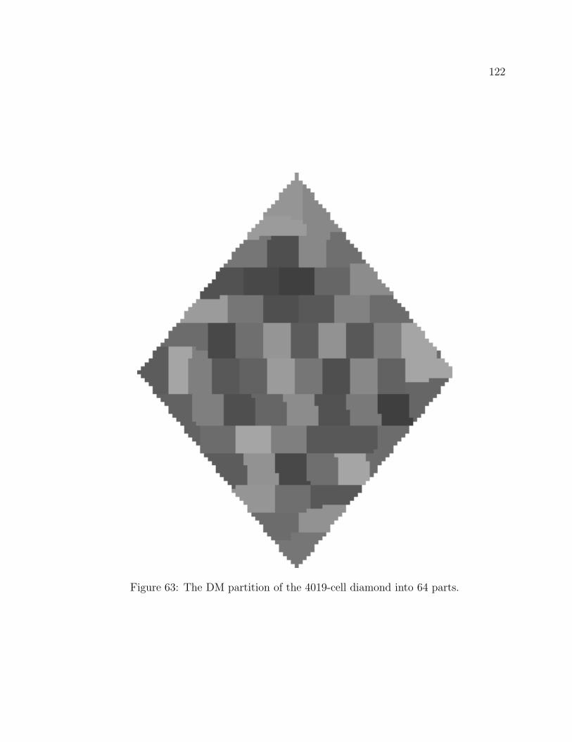
122
Figure 63: The DM partition of the 4019-cell diamond into 64 parts.

123
PerimetersShape Cells CM DM Lower Bound
(max. stripe height,max. observed height)
Ellipse 1083 1198 1188(20,5) 1142Ellipse 3305 2038 2016(20,9) 1920Ellipse 4329 2340 2300(20,12) 2176
Diamond 3279 2112 2076(20,12) 1920Diamond 5099 2608 2542(20,13) 2304Diamond 12959 4100 4058(25,20) 3712
Torus 4952 2532 2468(20,13) 2304Torus 7536 3098 3052(25,12) 2816Torus 10980 3740 3650(25,16) 3456
Table 7: CMR versus Donaldson-Meyer
In all cases, DM outperformed CMR. However, DM took much longer than CMR for
producing a result. CMR produces a solution very quickly. For a small problem (the
Ellipse problem with 1083 cells) CMR took less than 8 secs, while DM took three and
one-half minutes. For a big problem (the Diamond problem with 12959 cells), CM took
9 seconds; DM took about 3.7 hours.
One example that demonstrates the benefits of using the DM algorithm would be if
the same inter-processor-communication intensive process were to be run many times. If
the number of runs were great enough, then the additional time used by DM would be
made up by reduced total run-times for the process that used the DM partition.
As was shown earlier (Chapter 2), the GA methodology of Christou-Meyer did very
well when partitioning rectangular grids. As a check, the Donaldson-Meyer algorithm
was applied to the 100x100 grid with 8-way partition and the 128x128 grid with 128
components. The results of Donaldson-Meyer matched those of Christou-Meyer.
Because of the complexity of the assignments to the the U-turn region, if the number

124
of cells within a stripe is small it is not obvious if the common subproblem assumption
is valid. It then follows that different assigning patterns could produce different U-turn
regions.
To get around this problem, one could alter the assigning patterns to get a common
U-turn region. To ensure this common substructure the following steps could be taken.
1. Apply Assignment process 0 and determine the U-turn region.
The cells that are assigned during this phase will determine the U-turn
region for the remaining eight assignments.
2. Make the other eight assignments.
3. Save the best assignment.
The process in step 1 guarantees that each assignment technique deals with exactly
the same U-turn region.
6.5 Error Gaps
Since an approximation of Christou’s stripe-assignment pattern is one of the nine that is
tried, it is expected that CM’s error gap (distance to lower bound) should in general be
greater than those of DM.
To keep the running times down to reasonable levels, not all possible stripe heights
were considered for many of the problems presented in this dissertation. Theoretically,
if each component is to be assigned A cells, then under certain conditions, stripe heights
between 1 and A (actually, stripe heights between A and M, the total number of rows,
could also be considered) can be used to produce a feasible solution. But some stripe
heights were thought to not produce good solutions and were not considered.
125
A shape for a given area A that has optimal perimeter is a square with sides of length
A0.5. The shape of the enclosing rectangle for a given area can vary and still have optimal
perimeter. For the given problems the upper bounds on stripe heights were set so as to
fall outside of the range of stripe heights that would produce an optimal perimeter. It
is hoped that these choices for upper-bounds on stripe-heights are great enough so as to
not exclude desired results. Determination of stripe-height ranges is an area of future
research.
6.6 Summary
The numerical results presented in this section represent the best that can be achieved
using a stripe-based algorithm, for a given set of allowable stripe heights. These results
also confirm the effectiveness of the ideas of Yackel-Meyer (YM) and CM. CM, in par-
ticular, can produce a very good solution in a short amount of time (when considering
rectangular grids Martin [Mar96] also does an outstanding job).
The techniques described here could also be applied recursively to the U-turn re-
gion for a given stripe and the associated overflow cells in the next stripe. The U-turn
region and the associated overflow area form a grid graph with an integral number of
components.
The run-time of the software developed for this research is dependent on problem
parameters. For some of the bigger non-rectangular grids, the run-times were in the
minutes (and hours for big problems). In the future (see Chapter 7, section “Stripe-
height Range”), we plan to study the dependence of solution quality on the range of
stripe heights used.
There are three main data structures used in the implementation. The first is an

126
array containing the begin-end-row pairs that are valid stripes. The second is the actual
grid to be partitioned (also blocks of this overall grid, corresponding to stripes, must be
dynamically allocated). The third is the array used to store the dynamic-programming
results. The first data structure can easily be eliminated. It is not obvious how to get
around having in memory the entire grid to be partitioned, without depending on a fast
file system (i.e. reading from the hard disk just those parts of the grid that are to be
considered). Therefore, to work on problems of the size that Martin [Mar96] studied
(e.g. rectangular 1000 x 1000 grids) would probably require a substantial amount of
computing time.
Memory management is a major bottleneck in the current implementation. Using
the performance measuring tool Paradyn [MCC+95] on a moderately sized problem, it
appears that dynamically allocating some of the data structures may have the effect of
doubling the running time. In the future, we will explore the possibility of using static,
rather than dynamic, data structures.

127
Chapter 7
Conclusions, Contributions and
Future Work
7.1 Conclusions
For a large class of problems, stripe-based methodology has proven to be a very effective
approach for partitioning a grid graph. Intuitively, it is not hard to understand why
these algorithms perform well. These algorithms use a greedy approach to maximize the
number of components that have optimal or near-optimal perimeters. As long as the
components with non-optimal perimeters are not numerous (in a relative sense), overall
performance will be very good. In fact, total perimeter will approach the optimal value.
As a result of this research, we have shown that, under limited assumptions, that a
rectangular grid can be assigned so as to produce a locally optimal solution.
Previous methods used a simple approach for handling those components appearing
in two stripes. These methods could produce components that were far from optimal
and could easily be improved by swaps, resulting in a reduction of the total perimeter
for the overall assignment. This dissertation presented assignment techniques that would
reduce the occurrence of these bad assignments.
In the past, it was not feasible to determine the best set of stripe heights for gen-
eral domains. Under certain conditions, including rectangularity, of the domain, Martin

128
[Mar98] determines the best set of stripe heights, via a knapsack approach. (Because
of these limitations, it is not known if the problem that Martin solved was NP-Hard.)
Martin’s algorithm also did not allow overflow from one stripe to the next. By using
genetic algorithms, Yackel-Meyer [Yac93] and Christou-Meyer [CM96] find good sets
of stripe heights, without the restrictions imposed by Martin, but their solutions do not
guarantee an optimal set of stripe heights.
As a result of this research, it has been shown that there are a super polynomial
number of possible sets stripe heights; and for a given stripe assignment process, a
provably optimal set of stripe heights can be determined in a polynomial amount of
time.
7.2 Contributions
7.2.1 Improved Stripe Assignments and Local Optimality
For the case that an integral number of components are assigned to a stripe, as a result of
this research, it was shown that the assignment resulting from column-wise assignment
was locally optimal. Although these assignments were not always provably globally
optimal, the distance from the lower bound was guaranteed to be very small under
reasonable assumptions.
If stripe heights were chosen that did not allow an integral number of components,
then under the previous methodology, solutions contained assignments that could ob-
viously be improved. The previous algorithms only allowed for a single processor to
spillover across stripes. This led to the creation of peninsulas (a single row or column
of cells extending from the main body of cells assigned to the component), that could

129
be improved through a series of two-cell swaps, with the resulting assignment having a
better total perimeter. This dissertation presents algorithms that do not generate such
non-locally-optimal peninsulas.
The driving force behind these algorithms was the U-turn region. The U-turn re-
gion contains components that are assigned in more than one stripe and that also may
have an irregular shape that forces large perimeter values. So a balance must be struck
between the number of components assigned (in non U-turn regions) to near optimal con-
figurations and the components that will be assigned (in the U-turn region) to possibly
far-from-optimal configurations.
As a result of this research, nine basic assignment processes for the U-turn regions
For each single process, there exist configurations of unassigned cells that will lead to
poor results. However, in our experience, at least one of the nine performed relatively
well in every instance.
7.2.2 Exhaustive Searches are not Feasible
Before this research, the size of the set of feasible stripe-height sequences was not es-
tablished. It is now known that the size is at least super-polynomial in the number of
vertices. A brute-force exhaustive search is not feasible.
7.2.3 Defining Subproblems
The driving force behind all the breakthroughs in the second half of this dissertation is
the idea of defining subproblems that can be assigned independently of the remainder of
the domain. Through the use of three variables and a fixed stripe assignment process, a
subproblem can be uniquely defined and independently assigned. The remaining part of

130
the original domain is also assigned independently.
This idea is actually taken one step further. Individual stripes can be identified and
assigned independently of the rest of the grid. From this decomposition, two concepts
have emerged. The first is the idea of a stripe-quasi-independent (SQI) fill procedure.
For a given SQI fill procedure and a valid partial end-row sequence, the perimeter value
for subproblem (ei−1, ei, di) equals the perimeter value for the subproblem (ei−2, ei−1, (di
+ 1) mod 2) plus the perimeter for the components appearing before the corresponding
U-turn region for stripe i
The second concept is a stripe-fill optimal solution (SF). A SF solution is optimal
with respect to a set of feasible solutions obtained by:
1) specifying valid sequences of end-rows and
2) applying a SQI fill procedure.
7.2.4 Improved Stripe-Height Selection
The construction of a stripe-based partition can be thought of as incrementally append-
ing a stripe to one subproblem and producing another subproblem. Partitions of this
type posses the qualities of common subproblem and optimal substructure. These are
two qualities that are present in problems for which dynamic programming and greedy
algorithms are applicable. By being able to consider appropriate subproblems, both of
these algorithms exploit these qualities and organize the results in such a way as to
eliminate redundant and a potentially super-polynomial number of calculations.
For the greedy algorithm approach, the original problem is transformed into a state
graph, with one source node (corresponding to an unassigned grid) and one sink node
(corresponding to an assigned grid). Each node in the graph corresponds to a subproblem.
An edge exists between node (b,e,d) and (b’,e’,d’) if and only if a valid stripe can be

131
appended to the subproblem defined by (b,e,d) to get (b’,e’,d’). The shortest path from
the source to a node corresponds to an optimal partition of the corresponding subproblem.
The shortest path from the source to the sink corresponds to an optimal partition in the
original grid.
An optimal solution can be represented as a sequence of stripe heights and fill direc-
tions. Consider the last stripe. There are a finite number of possible final stripes. We
know that the stripe height for the optimal solution must come from this set. If the final
stripe corresponding to the optimal partition is stripped away, the problem remaining is
a smaller version of the original problem. The partition for this smaller problem must
also be optimal, or else the optimal partition could be added to the final stripe to produce
a better overall solution.
This mechanism is contained in the following recurrence:
P(i,j,d) = minb(perim(b,i,j,d) + P(b,i-1,(d+1) mod 2))
Taking into account the termination conditions and multiple stripe-assignment pro-
cesses, this is the recurrence that our implementation uses.
7.3 Future Work
7.3.1 Post-Processing
As was mentioned earlier, a locally optimal solution can be improved if multi-cell (more
than 2) swaps are allowed. The partition in figure 52 is locally optimal, but is not globally
optimal. The key is trying to identify the expanded sets of cells to be swapped.
One method of post processing would be to use the Kernighan-Lin heuristic that
allows for a sequence of swaps, in which any individual swap in the sequence may not

132
necessarily improve the solution, but taken as a whole, the sequence of swaps does.(A
worsening swap may perturb the assignments enough to create several other improv-
ing swaps) Swap-cell selections would be based on priorities determined by perimeter
contributions.
Another post-processing technique to be studied will be border swapping. In figure 52,
the borders for the 1’s and 2’s could be reassigned to get a better solution. Also, the
assignment processes will be used to post-process poor quality U-turn regions and any
stripes whose components are not of good quality.
7.3.2 Stripe-Height Range
The range of heights that a stripe may assume plays a major role in the amount of time
required to generate an optimal set of stripe heights. As was mentioned earlier, for some
of the bigger problems it took hours to generate the optimal set of stripe heights. Further
study is needed on how total perimeter is affected by reductions in the set of heights that
a stripe may assume.
7.3.3 Extension to the 3-D case
To extend the stripe-selection process to the 3-D grid graphs only requires a modification
as to how a subproblem is to be defined. Figure 64 shows how a a 3-D graph might be
divided into four “slices”.
To make the diagrams a little easier to construct and to follow, only parallel pipettes
will be considered. If some other type of 3-D grid were to be examined, the slicing would
be done on the enclosing parallel pipette for the graph. The first two variables in any
recurrence would then be the beginning and ending rows for the slice.

133
Within these slices, configurations approximating cubes will be packed in columns.
Figure 64 shows the first column of near-cubes assigned within a stripe. This packing
of cubes will continue in a manner similar to the striping done in the 2-D case. There
are several different sequences of column widths that would have to be examined and
organized just like in the 2-D case.
As in the 2-D case, if the last row within a 3-D subproblem is known, then the total
number of complete components that may be assigned within the corresponding volume
can be determined. By knowing the height of the last slice, the width and direction of
assignment of the last groups of cubes packed within the slice, the configuration of cells
to be assigned becomes independent of the how the previous slices were assigned.
For handling overflow from one slice to the next see figures 65 and 66
7.3.4 Parallel Computing
For all of the methodology concerning stripe selection, it was assumed that (although
unstated) we had chosen the best orientation for the 2-D grid; this may not be the
case. If the grid is not symmetric about both axes, then it might actually be better to
use another corner as the starting point. Since there are a constant number of different
starting points (four corners, when considering the enclosing frame), this type of problem
lends itself to parallel computing. One way to divide up the problem is to assign each
starting corner-point to a different processor. A more sophisticated variant would add a
pool of post-processing tasks that could be processed in parallel. This type of distribution
of work could also be extended to the 3-D case, where 24 processors could be used.

134
A
B
C
D
A
B
C
D
Figure 64: Slicing a 3-D grid

135
Unassigned cells
1 2 3
123
View of top from above
Figure 65: Assigning columns within a slice

136
Figure 66: A configuration of unassigned cells

137
7.4 Summary
As a result of this research, both phases of stripe-based partitioning algorithms have
been improved. The method of stripe assignment has been improved to guarantee locally
optimal solutions in the rectangular case, and high-quality solutions in the general case.
Previous research focussed on heuristics or restrictive approaches to select sequences of
stripe heights. As a result of this research, there now exist efficient polynomial algorithms
that produce the best sequence of stripe heights.

138
Bibliography
[ANO] ANONYMOUS. A manpage provided through the operating system used at
the University of Wisconsin-Madison.
[Chr96] I. Christou. Distributed Genetic Algorithms for Partitioning Uniform Grids.
PhD thesis, University of Wisconsin - Madison, August 1996.
[CLR90] T. H. Cormen, C. E. Leiserson, and Ronald L. Rivest. Introduction to Algo-
rithms. McGraw-Hill, New York, 1990.
[CM95] I. T. Christou and R. R. Meyer. Optimal and Asymtotically Optimal Equi-
partition of Rectangular Domains via Stripe Decomposition. University of
Wisconsin Mathematical Programming Technical Report, 95-19, 1995.
[CM96] I. T. Christou and R. R. Meyer. Optimal equi-partition of rectangular do-
mains for parallel computation. Journal of Global Optimization, 8:15–34,
January 1996.
[DM99] W.W. Donaldson and R.R. Meyer. A Dynamic-Programming Approach for
Grid-Graph Partitioning. 1999. Manuscript.
[Don97] W.W. Donaldson. Locally Optimal Striping for Rectangular Grids.
Manuscript, 1997.
[FGK93] R. Fourer, D. M. Gay, and B. W. Kernighan. AMPL: A Modeling Language
for Mathematical Programming. The Scientific Press, 1993.
[Fra99] ILOG SA France. CPLEX Linear Optimizer 6.5.1. 1997-1999.
[GJ79] M. R. Garey and D. S. Johnson. Computers and Intractability: A Guide to
the Theory of NP-Completeness. W.H. Freeman, 1979.
[GMSJ93] S. Ghandeharizadeh, R.R. Meyer, G. Schultz, and J.Yackel. Optimal balanced
partitions and a parallel database application. ORSA Journal on Computing,
4:151–167, 1993.
139
[GMT95] J. R. Gilbert, G. L. Miller, and S. H. Teng. Geometric mesh partitioning:
Implementation and experiments. In Proceedings of the 9th International
Symposium on Parallel Processing, pages 418–427, 1995.
[Gol89] D. E. Goldberg. Genetic Algorithms in Search, Optimization and Machine
Learning. Addison–Wesley, Reading MA, 1989.
[HL95a] B. Hendrickson and R. Leland. The Chaco User’s Guide Version 2.0. Sandia
National Laboratories, July 1995.
[HL95b] B. Hendrickson and R. Leland. An improved spectral graph partitioning
algorithm for mapping parallel computations. SIAM J. on Sci. Comput.,
16:452–469, 1995.
[Hol92] John Holland. Adaptation in Natural and Artificial Systems. MIT Press,
1992.
[KK95a] G Karypis and V. Kumar. A fast and high quality multilevel scheme for
partitioning irregular graphs. Technical Report TR 95-037, Dept. of Computer
Science, Univ. of Minnesota, 1995.
[KK95b] G Karypis and V. Kumar. A fast and high quality multilevel scheme for
partitioning irregular graphs. Technical Report TR 95-035, Dept. of Computer
Science, Univ. of Minnesota, 1995.
[KK95c] G. Karypis and V. Kumar. Metis: Unstructured graph partitioning and sparse
matrix ordering system. 1995.
[KK95d] G Karypis and V. Kumar. Multilevel k-way partitioning scheme for irregular
graphs. Technical Report TR 95-064, Dept. of Computer Science, Univ. of
Minnesota, 1995.
[KL70] B. W. Kernighan and S. Lin. An effective heuristic procedure for partitioning
graphs. Bell Systems Tech. Journal, pages 291–308, February 1970.
[Mar96] W. Martin. Fast equi-partitioning of rectangular domains using stripe decom-
position. Technical Report MP-TR-96-2, University of Wisconsin - Madison,
February 1996. to appear in Discrete Applied Mathematics.

140
[Mar98] W. Martin. Fast equi-partitioning of rectangular domains using stripe de-
composition. Discrete Applied Mathematics, 82:193–207, 1998.
[MCC+95] B. P. Miller, M. D. Callaghan, J. M. Cargille, J. K. Hollingsworth, R. B.
Irvin, Karen L. Karavanic, K. Kunchithapadam, and T. Newhall. The para-
dyn parallel performance measurement tools. IEEE Computer 28, 11:37–46,
November,1995.
[Mey99] R.R. Meyer. Class notes for CS 720 at the University of Wisconsin-Madison.
1999.
[Mic94] Z. Michalewicz. Genetic Algorithms + Data Structures = Evolution Programs.
Springer-Verlag, 1994.
[MT90] S. Martello and P. Toth. Knapsack Problems: Algorithms and Computer
Implementations. Wiley, 1990.
[MTTV93] G. L. Miller, S. H. Teng, W. Thurston, and S. A. Vavasis. Automatic mesh
partitioning. In A. George, J. R. Gilbert, and J. W. H. Liu, editors, Graph
Theory and Sparse Matrix Computation, pages 57–84. Springer-Verlag, 1993.
[NW85] G. Nemhauser and L. Wolsey. Integer and Combinatorial Optimization. John
Wiley & Sons, 1985.
[Sch89] R. J. Schalkoff. Digital Image Processing and Computer Vision. John Wiley
& Sons, 1989.
[ST93] H. D. Simon and S. H. Teng. How Good is Recursive Bisection. 1993.
[Str89] J. Strikwerda. Finite Difference Schemes and Partial Differential Equations.
Wadsworth & Brooks, 1989.
[Yac93] J. Yackel. Minimum Perimeter Tiling in Parallel Computation. PhD thesis,
University of Wisconsin - Madison, August 1993.
[YMC97] J. Yackel, R. R. Meyer, and I. Christou. Minimum-perimeter domain assign-
ment. Mathematical Programming, 78:283–303, 1997.