Re-Envisioning the Ocean:The View from Space

Mark R. AbbottCollege of Oceanic and Atmospheric Sciences

Oregon State University

Introduction

• It was once said that the “G” in JGOFS would not be achieved until an ocean color sensor was launched

• But the first research-quality sensor was not launched until 1996!

• However, many other sensors were available during JGOFS for ocean research

• These came about from a confluence of proposed satellite missions and global ocean research in the early 1980’s

The Keystone Year - 1978

• Seasat - the “100-day” mission– Radar altimeter– Scatterometer– SAR– Passive microwave radiometer

• TIROS-N– Advanced Very High Resolution Radiometer

• Nimbus-7– Coastal Zone Color Scanner– Passive microwave radiometer

Preparing for the Next Missions

• 1978 missions showed great promise for ocean research

• Standard practice to begin building support for new missions right away

• WOCE and beyond– Dynamic topography, mesoscale variability

• TOPEX/POSEIDON, ERS-1, ERS-2, Jason-1– Wind stress

• ERS-1, ERS-2, ADEOS-1 (NSCAT), QuikSCAT, Envisat, ADEOS-2 (SeaWinds)

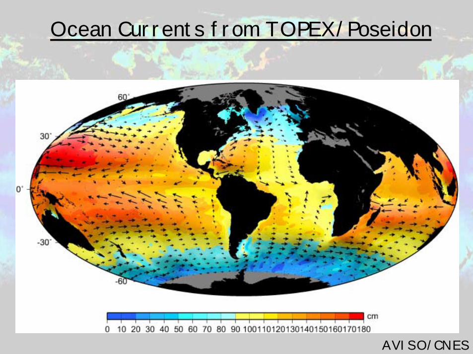
Ocean Currents from TOPEX/Poseidon

AVISO/CNES

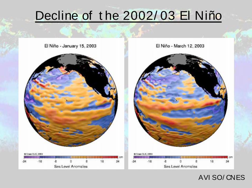
Decline of the 2002/03 El Niño

AVISO/CNES

Global Wind Field

D. Chelton (OSU)

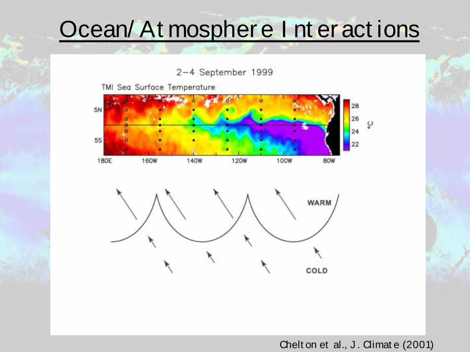
Ocean/Atmosphere Interactions

Chelton et al., J. Climate (2001)

How Vector Winds Respond

Chelton et al., J. Climate (2001)

An Animation of Vector Winds and SST

Chelton et al., J. Climate (2001)

Curl and Divergence

D. Chelton (OSU)

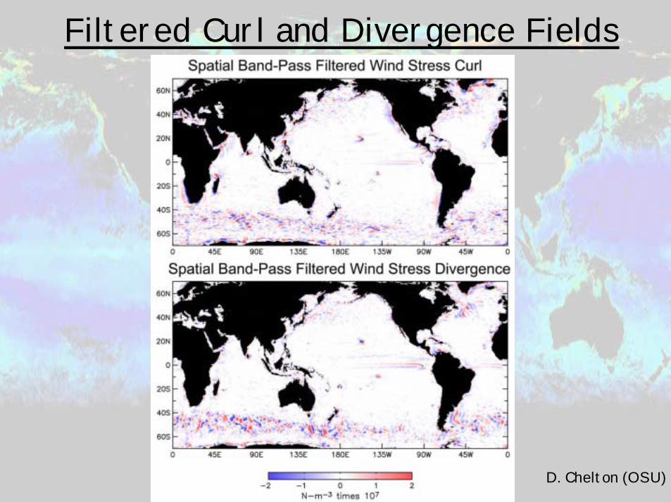
Filtered Curl and Divergence Fields

D. Chelton (OSU)

Ekman Upwelling Velocity

Estimates

M. Freilich (OSU)

Mesoscale Variability

Wind shadow adjacent to South Georgia Island

M. Freilich (OSU)

“Operational” Sensors for Ocean Research

• Infrared – AVHRR– Series begun in 1978– JPL/NASA/NOAA global reprocessing for

period 1987-1999• Passive microwave – SSM/I

– Series begun in 1987– Sea ice, wind speed, atmospheric properties– Lower frequencies on Tropical Rainfall

Measuring Mission (TRMM) to measure SST

Can We Use Satellites to Study Long Time Scale Processes?

• “Operational” satellites (those designed primarily for short-term forecasting needs and other mission-critical functions)– Polar-orbiters such as those operated by NOAA

(POES) and US Dept. of Defense (DMSP)– Time series of SST and water vapor (Frank

Wentz, Remote Sensing Systems• Some research satellites have now

generated long time series• An example from the Southern Ocean

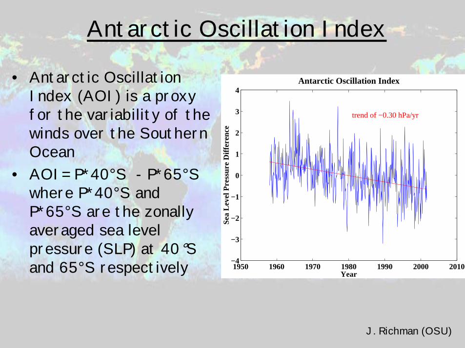
Antarctic Oscillation Index

• Antarctic Oscillation Index (AOI) is a proxy for the variability of the winds over the Southern Ocean

• AOI= P*40°S - P*65°S where P*40°S and P*65°S are the zonallyaveraged sea level pressure (SLP) at 40°S and 65°S respectively 1950 1960 1970 1980 1990 2000 2010

−4

−3

−2

−1

0

1

2

3

4

Year

Sea

Lev

el P

ress

ure

Diff

eren

ce

Antarctic Oscillation Index

trend of −0.30 hPa/yr

J. Richman (OSU)

Zonal Winds in the NCAR/NCEP Reanalysis

J. Richman (OSU)

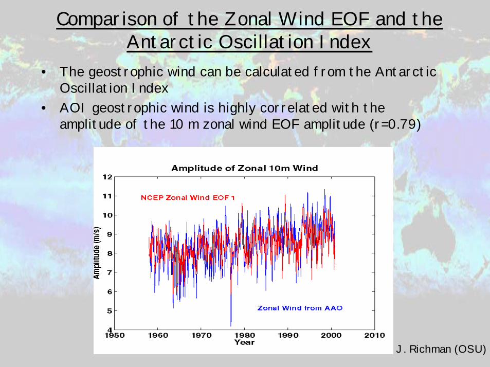
Comparison of the Zonal Wind EOF and the Antarctic Oscillation Index

• The geostrophic wind can be calculated from the Antarctic Oscillation Index

• AOI geostrophic wind is highly correlated with the amplitude of the 10 m zonal wind EOF amplitude (r=0.79)

J. Richman (OSU)

Interannual Changes in Wind Forcing

J. Richman (OSU)

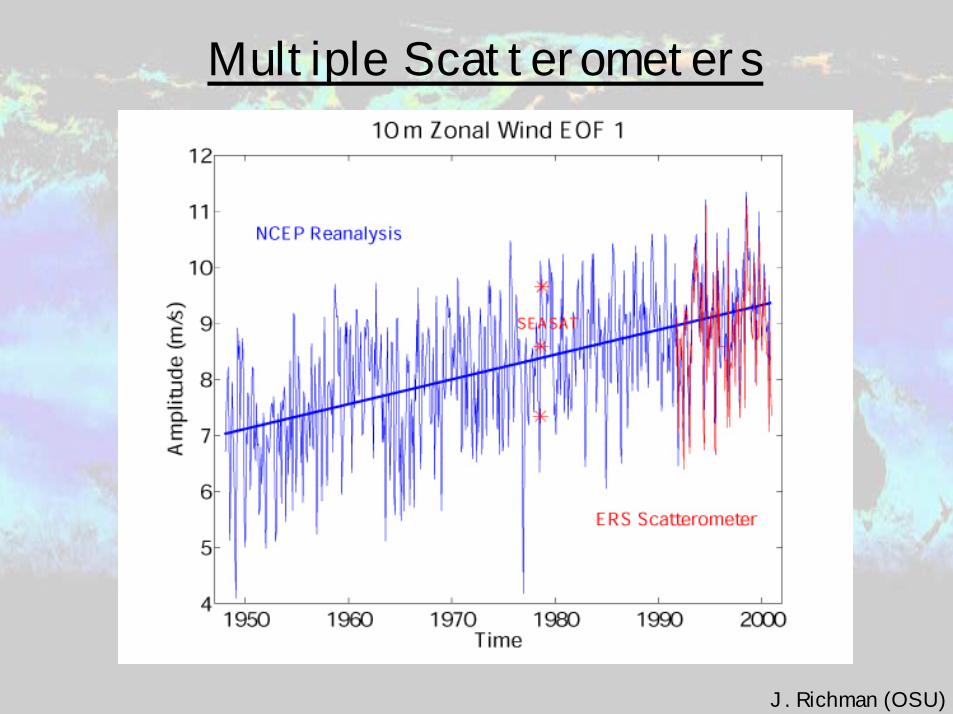
Multiple Scatterometers

J. Richman (OSU)

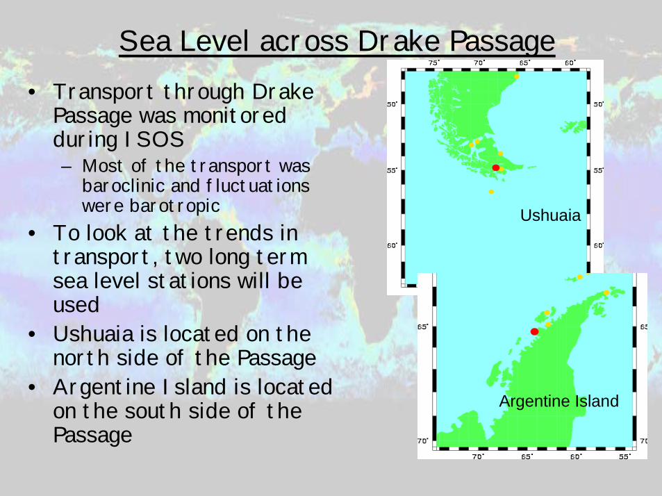
Sea Level across Drake Passage• Transport through Drake

Passage was monitored during ISOS – Most of the transport was

baroclinic and fluctuations were barotropic

• To look at the trends in transport, two long term sea level stations will be used

• Ushuaia is located on the north side of the Passage

• Argentine Island is located on the south side of the Passage

Ushuaia

Argentine Island

Transport and Sea Level Difference across Drake Passage

• The sea level difference across the Passage shows a trend of -0.62 cm/year

• Assuming that the transport fluctuations are barotropic with a 2.25 Sv/cm and transport of 123 Sv in 1980, the modeled transport has a trend of 1.4 Sv/year increasing from 110 Sv in 1970 to 150 Sv at present

1970 1975 1980 1985 1990 1995 2000-0.2

-0.15

-0.1

-0.05

0

0.05

0.1

0.15

0.2

0.25

Year

Sea L

evel

Diffe

rence

(m)

Trend of -0.62 cm/year

Sea Level Difference Across Drake Passage

1970 1975 1980 1985 1990 1995 200060

80

100

120

140

160

180

Year

Trans

port f

rom Se

a Lev

el Dif

feren

ce (S

v)

Transport through Drake Passage

Trend of 1.4 Sv/year

J. Richman (OSU)

Summary of Long-Term Changes in the Southern Ocean

• Winds over the Southern Ocean from the NCAR/NCEP Reanalysis show a trend of 4.4 cm/s/yr increasing from a mean of 7 m/s to 9.2 m/s over 53 years, – This represents a 50% increase in the wind stress

• Satellite scatterometers show a similar trend of 3.9 cm/s/yr in the 1990s and the 3 months of SEASAT in 1979 are consistent with the long term trend

• Drake Passage transport shows an increase of 1.4 Sv/yr corresponding to an increase from 123 Sv in 1980 to 150 Sv in 2000

Impacts

• Increasing winds will increase transport• But observed transport does not increase

sufficiently to account for increased wind-driven transport

• Increased vertical transport of momentum via eddies is one possibility

• How well do models capture eddy processes?

Models Underestimate Sea Level Variability

Ocean Color Satellites

• Strong connections with JGOFS, building on success of CZCS

• Recent missions– OCTS – on ADEOS-1 (1996-1997)– SeaWiFS – on ORBIMAGE (1997 – present)– MODIS – on EOS-Terra (1999 – present) and

EOS-Aqua (2002 – present)– MERIS – on Envisat (2002 – present)– GLI – on ADEOS-2 (2002 – present)

• Research missions– High quality sensors, algorithms– Strong science involvement

Where Did We Start?

• Global Ocean Flux study (1984)– Satellite/Surface Productivity group

• McCarthy, Abbott, O. Brown, Eppley, Flierl, Gagosian, Minster, Morel, Pollard, R. Smith, Walsh, and Yentsch

• Recommendations included:– Routine measurements of ocean color, SST– Development of optical buoys (about 70)– Relate surface and subsurface properties– Design of optimal sampling strategies– Coordination with field programs– Development of coupled global models – Development of scientific infrastructure

And What Did We Hope to Achieve?

“Prognostic models...must have adequate parameterization of small-scale processes. Such models should be able to predict the biological response to physical forcing. Moreover, the statistical properties of these models must be correct. That is, they should be able to predict the spatial and temporal variability of processes such as carbon flux in response to variable physical processes, both oceanic and atmospheric. Such modeling efforts will require sophisticated computational techniques to incorporate global pigment and SST data as well as wind and altimetricdata.” (NRC 1984)

Annual Mean Chlorophyll

Moore and Abbott, JGR

(2000)

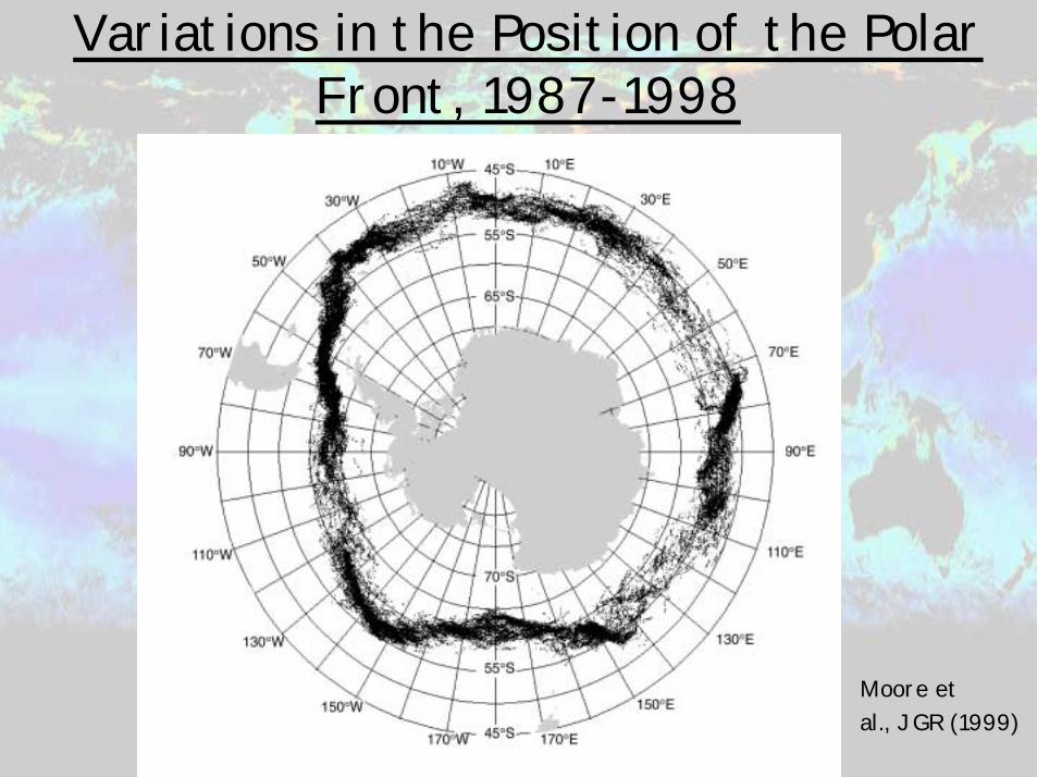
Variations in the Position of the Polar Front, 1987-1998

Moore et al., JGR (1999)

•Steering of Polar Front by bottom topography•Meanders more common where topography is flat

Moore et al., JGR (1999)

Spatial Statistics from Ocean Color

Doney et al., JGR (2003)

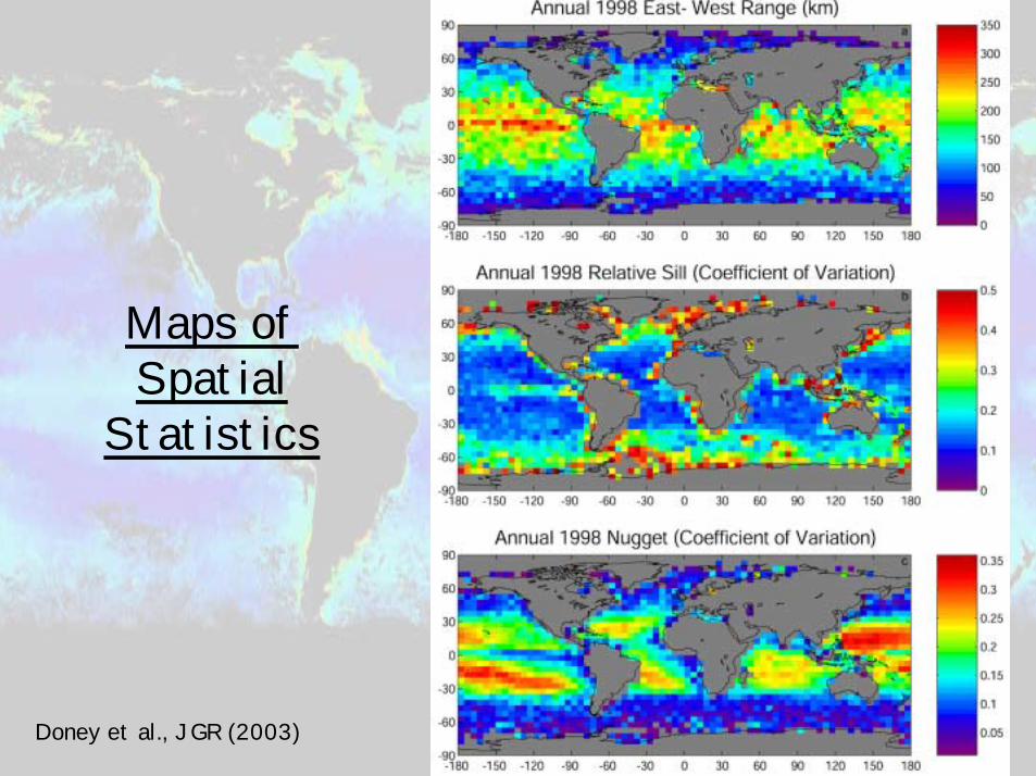
Maps of Spatial

Statistics

Doney et al., JGR (2003)

SeaWiFS Sampling at the Polar Front

Primary Productivity Round Robin

Campbell et al., GBC (2002)

Estimates of Primary Productivity

29.7Walsh (1988)27.0Berger (1989)51Martin et al. (1987)

48.5Behrenfeld and Falkowski (1997)45-50 Pg C/yrLonghurst et al. (1995)GlobalStudy

Most of the variability in estimates is due to the uncertainty in the physiological parameters in the models

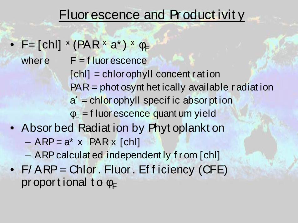
Fluorescence and Productivity

• F= [chl] x (PAR x a*) x φFwhere F = fluorescence

[chl] = chlorophyll concentrationPAR = photosynthetically available radiationa* = chlorophyll specific absorptionφF = fluorescence quantum yield

• Absorbed Radiation by Phytoplankton– ARP = a* x PAR x [chl]– ARP calculated independently from [chl]

• F/ARP = Chlor. Fluor. Efficiency (CFE) proportional to φF

Aircraft Measurements of FLH Compared with MODIS over the Gulf Stream

Hoge et al., Appl. Opt. (2003)

Field Measurements of Chlorophyll and MODIS

-Blue = all mesoscale survey data-Red = Within 0.5 days of the MODIS Image Time stamp

In situ chl (mg m-3) In situ chl (mg m-3)

MO

DIS

chl

_2 (m

g m

-3)

MO

DIS

FLH

, W m

-2um

-1sr

-1

Chlorophyll FLH

PP = [chl] x (PAR x a*) x Φp (1)If Φp + Φf + Φh = 1 & Φh = constant

then Φp = constant – Φf (2)

Replacing Φp with (2) in (1)

PP = [chl] x (PAR x a*) x (constant – Φf)

or PP α ARP x (constant - FLH/ARP) α (constant/ARP) - FLH

Can we use MODIS CFE to improve the Primary Productivity algorithm?

MODIS_Chl MODIS_FLH MODIS_CFE MODIS_ARP

OSU Direct Broadcast October 04, 2001

MODIS data shows chl not always in spatial correspondence with fluorescence Physiological parameters also vary spatially

0.2

0.4

0.6

0.8

1

1.2

45 ° N

44 ° N

43 ° N

42 ° N

41 ° N

123 ° W 124 ° W 125 ° W 126 ° W 127 ° W

Coos Ba y

Ne w port

Cape Bla nc o

He c e ta Hea d

Latit

ude

Longitude

PP/PS

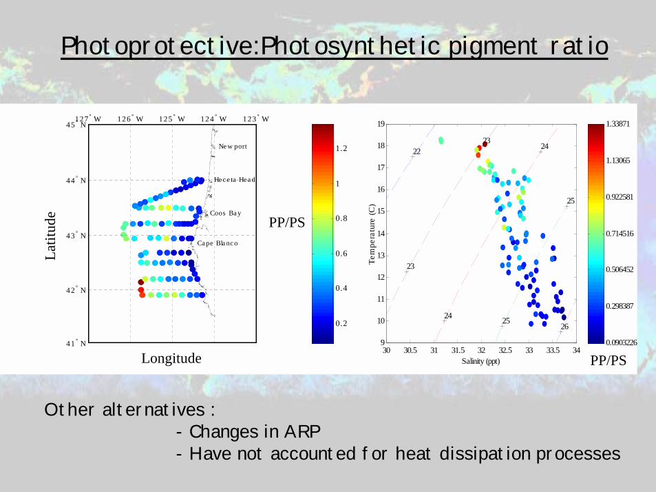
Photoprotective:Photosynthetic pigment ratio

0.0903226

0.298387

0.506452

0.714516

0.922581

1.13065

1.33871

30 30.5 31 31.5 32 32.5 33 33.5 349

10

11

12

13

14

15

16

17

18

19

262524

23

2223

24

25

Salinity (ppt)Te

mpe

ratu

re (C

)PP/PS

Other alternatives : - Changes in ARP - Have not accounted for heat dissipation processes

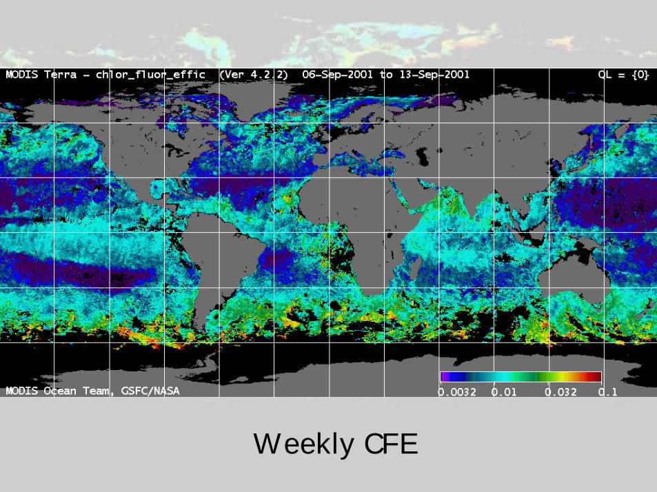
Weekly CFE

MODIS Chlorophyll Time Series

HOT AESOPS

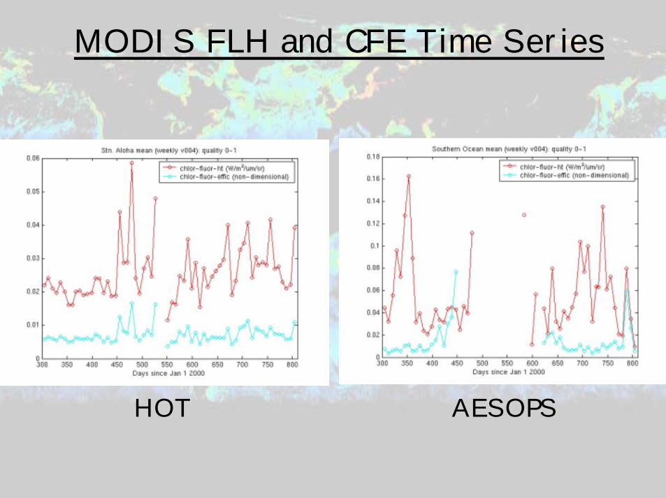
MODIS FLH and CFE Time Series

HOT AESOPS

0

0.005

0.01

0.015

0.02

0.025

0.03

0.035

0.04

0.045

0.05

0 0.1 0.2 0.3 0.4 0.5 0.6 0.7 0.8 0.9 1

0

0.1

0.2

0.3

0.4

0.5

0.6

0 0.1 0.2 0.3 0.4 0.5 0.6 0.7 0.8 0.9 1

Fv/F

m, n

.d.

9 A

M C

FE, r

.u.

µ/µmax , n.d.

Thalassiosira weissflogiiChemostat results 2001-2002

After 3 days of constant cell counts

After 14 days

Summary of Fluorescence and Productivity

• Fluorescence and chlorophyll– Generally a linear relationship between absorption-

based estimates and fluorescence-based estimates of chlorophyll

• Exceptions are apparent, for example near the coast– Slope of line relating FLH to chl is related to CFE

• Fluorescence and productivity– Challenge is that many processes affect φF

• Photoprotective pigments, absorption cross-section– Appears, though, that CFE appears to fall into 2

clusters so problem may be tractable– High values of CFE appear to be associated with

communities far from equilibrium• Time history of CFE may be key

Putting It All Together

• Interactions between wind forcing and mesoscale ocean processes– Affects vertical and horizontal fluxes

• Long-term shifts in wind forcing can impact mesoscale processes

• Strong biological/physical coupling at mesoscales• Satellite measurements of fluorescence may help

identify areas where phytoplankton are not in equilibrium with light/nutrient regime

• Good prospects for improving estimates of primary productivity

• Satellites will always “miss” some scales and some processes

Future Directions

• Programs such as CLIVAR, GODAE, and GOOS emphasize operational observation strategy

• But programs such as JGOFS have shown that much research remains, especially in ecology and physical coupling– What processes need to be included?– What scales do we need to observe?– How do we parameterize for models?– Many of these remain as challenges from 1984

• Are ocean sciences ready?– We do need long-term, carefully-calibrated series

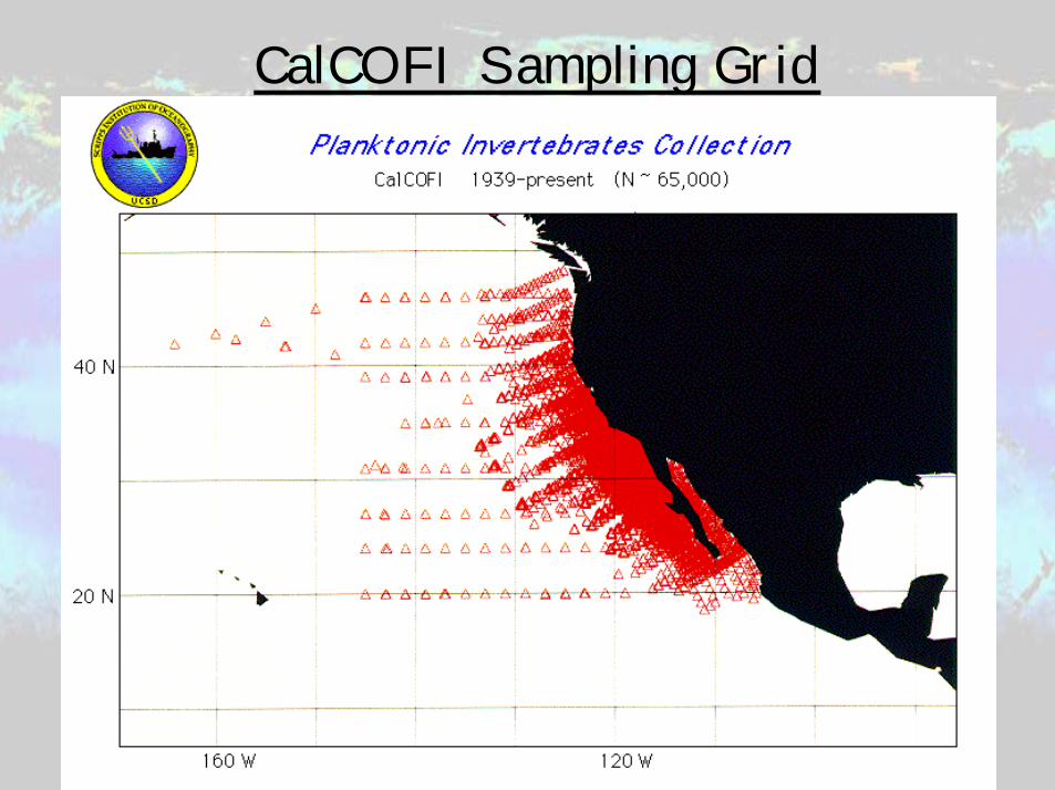
CalCOFI Sampling Grid

Despite 40 years’ of sampling, CalCOFI missed one of the dominant features of the California Current!

Acknowledgments

• Dudley Chelton, Steve Esbensen, Larry O’Neill, and Mike Freilich

• Jim Richman and Yvette Spitz• Ricardo Letelier, Jasmine Nahorniak, and

Amanda Ashe, Rachel Sanders, and Claudia Mengelt

• Keith Moore