Rank Efficiency: Investigating a Widespread

Ordinal Welfare Criterion

Clayton R. Featherstone∗

December 10, 2013

UNDER REVISION: COMMENTS WELCOME

Abstract

Many institutions that allocate scarce goods based on rank-order preferencesgauge the success of their assignments by the resulting rank distributions, thatis, how many participants get their first choice, how many get their secondchoice, and so on. For example, San Francisco Unified School District, Teachfor America, and Harvard Business School all evaluate assignments in this way.Preferences over rank distributions capture the practical (but non-Paretian)intuition that hurting one agent to help others might be desirable. Motivatedby this, call an assignment rank efficient if its rank distribution cannot feasiblybe stochastically dominated. Rank efficient mechanisms are simple linear pro-grams that can either be solved all at once by a computer or through an intuitivesequential improvement process where at each step, the policy-maker executesa potentially non-Pareto-improving trade cycle. Both methods are used in thefield. Rank efficiency also dovetails nicely with previous literature: it is a re-finement of ordinal efficiency (and hence of ex post efficiency). Although rankefficiency is theoretically incompatible with strategy-proofness, rank efficientmechanisms can admit a truth-telling equilibrium in low information environ-ments. Preference data from Featherstone and Roth (2011) show that if agentswere to truthfully reveal their preferences, a rank efficient mechanism couldsignificantly outperform commonly considered alternatives like random serialdictatorship and the probabilistic serial mechanism. Finally, a competitiveequilibrium mechanism like that of Hylland and Zeckhauser (1979) generatesa straightforward generalization of rank efficiency and sheds light on how rankefficiency interfaces with fairness considerations.

∗The Wharton School, University of Pennsylvania

1

1 Introduction

Mechanisms that map submitted ordinal preferences into an assignment of agents to

objects are common, and institutions that use them often gauge success by looking

at rank distributions, that is, at how many participants get their first choice, how

many get their second choice, and so on. For example, when school districts announce

the results of a choice-based student placement system, they report things like how

many students were assigned to one of their top three choices and how many were

unmatched (NYC Department of Education 2009, San Francisco Unified School Dis-

trict 2011).1 Another example is the mechanism used by Teach for America to match

teachers to regions, which explicitly selects an assignment based on rank distribu-

tion.2 And finally, consider the strategy-proof random serial dictatorship used by

Harvard Business School to match MBAs to the country in which they fulfill their

global immersion requirement.3 In the first year the mechanism was run, administra-

tors were so concerned about the number of students who, in spite of ranking it last,

were assigned to an unpopular country, that they seriously considered exchanging

those students with others who had only given the unpopular country a moderately

low rank. After being reminded that such rearrangement would violate a promise of

strategy-proofness, they reluctantly stayed with the original assignment. Indeed, a

big part of strategy-proofness is making it safe for agents to reveal that they somewhat

like objects that most other agents strongly dislike.

This last anecdote is not surprising in light of the fact that random serial dicta-

torship is merely Pareto efficient. It could easily yield an assignment where shifting

one student from first to second choice could enable four other students to shift from

second to first choice.4 While this sort of trade seems good for overall welfare, Pareto-

agnosticism only insists on trades that weakly improve all agents. Motivated by this

common-sense intuition and encouraged by the widespread use of rank distribution-

based objectives in the field, define a feasible assignment to be rank efficient if its

rank distribution cannot be first-order stochastically dominated by that of another

1SFUSD also made frequent use of rank distributions to help them understand how to comparedifferent school choice mechanisms proposed by myself, Atila Abdulkadiroglu, Muriel Niederle, ParagPathak, and Al Roth over the course of the 2009-2010 school year in which we advised them.

2Teach for America is a nationwide non-profit that sends mostly new college graduates to teachin at-risk public schools. Al Roth and I are actively involved with helping the organization tostreamline its assignment process. See Section 4.4 for more.

3This paper discusses the HBS global immersion match in Section 7. Al Roth and I are activelyinvolved with the design of the match. See Featherstone and Roth (2011).

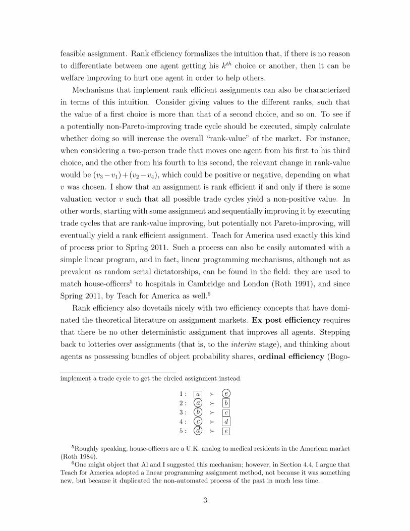
4Consider the following five agent, five position example, where the circles and boxes representtwo different assignments. A policy-maker looking at the boxed assignment might be tempted to

2

feasible assignment. Rank efficiency formalizes the intuition that, if there is no reason

to differentiate between one agent getting his kth choice or another, then it can be

welfare improving to hurt one agent in order to help others.

Mechanisms that implement rank efficient assignments can also be characterized

in terms of this intuition. Consider giving values to the different ranks, such that

the value of a first choice is more than that of a second choice, and so on. To see if

a potentially non-Pareto-improving trade cycle should be executed, simply calculate

whether doing so will increase the overall “rank-value” of the market. For instance,

when considering a two-person trade that moves one agent from his first to his third

choice, and the other from his fourth to his second, the relevant change in rank-value

would be (v3−v1)+(v2−v4), which could be positive or negative, depending on what

v was chosen. I show that an assignment is rank efficient if and only if there is some

valuation vector v such that all possible trade cycles yield a non-positive value. In

other words, starting with some assignment and sequentially improving it by executing

trade cycles that are rank-value improving, but potentially not Pareto-improving, will

eventually yield a rank efficient assignment. Teach for America used exactly this kind

of process prior to Spring 2011. Such a process can also be easily automated with a

simple linear program, and in fact, linear programming mechanisms, although not as

prevalent as random serial dictatorships, can be found in the field: they are used to

match house-officers5 to hospitals in Cambridge and London (Roth 1991), and since

Spring 2011, by Teach for America as well.6

Rank efficiency also dovetails nicely with two efficiency concepts that have domi-

nated the theoretical literature on assignment markets. Ex post efficiency requires

that there be no other deterministic assignment that improves all agents. Stepping

back to lotteries over assignments (that is, to the interim stage), and thinking about

agents as possessing bundles of object probability shares, ordinal efficiency (Bogo-

implement a trade cycle to get the circled assignment instead.

1 : a e©2 : a© b

3 : b© c

4 : c© d

5 : d© e

5Roughly speaking, house-officers are a U.K. analog to medical residents in the American market(Roth 1984).

6One might object that Al and I suggested this mechanism; however, in Section 4.4, I argue thatTeach for America adopted a linear programming assignment method, not because it was somethingnew, but because it duplicated the non-automated process of the past in much less time.

3

molnaia and Moulin 2001) requires that there be no other assignment of shares that

stochastically improves all agents. Rank efficiency is a refinement of both concepts.7

Looking to mechanisms, random serial dictatorship8 is ex post efficient, strategy-

proof, and ubiquitous in the field, while the probabilistic serial mechanism9 is or-

dinally efficient, generically non-strategy-proof, and absent in the field. Given the

theoretical appeal of ordinal efficiency, it was unclear why there are no ordinally ef-

ficient mechanisms in the field. Since rank efficient mechanisms are also ordinally

efficient, however, their presence resolves this institutional puzzle.

In the field, the conflict between strategy-proofness and refined efficiency is framed

as a decision between random serial dictatorship and linear programming. How does

the market designer choose which mechanism is the right one? Do rank efficient mech-

anisms ever make sense, or are they “mistakes” made by uninformed policy-makers?

Two exercises inform these concerns. First, in low information environments, like

those of Roth and Rothblum (1999), rank efficient mechanisms admit a truth-telling

equilibrium. This is how Teach for America justifies using a potentially manipulable

linear programming mechanism: teachers only apply once, are geographically sepa-

rated, and know little about what regions are popular and how the mechanism is run.

The second exercise uses empirical data (Featherstone and Roth 2011) from Harvard

Business School’s strategy-proof global immersion match. Under truth-telling, a rank

efficient mechanism yields more than a 15% improvement in the number of MBAs

who are assigned to a first or second choice country (out of 11) when compared to the

assignment given by random serial dictatorship. Although these gains might be un-

dermined by strategic preference manipulation, the exercise shows that in a naturally

occurring environment, the costs of strategy-proofness can be quite large. Together,

these exercises indicate that in certain environments, it would be a mistake to not at

least consider using a rank efficient mechanism.

Finally, the paper considers a class of ordinal mechanisms based on Hylland and

Zeckhauser (1979). These mechanisms assume cardinal preferences to rationalize the

submitted ordinal preferences, give each agent a budget of artificial10 money, and

7Given the limited information of an ordinal setting, one can interpret rank efficiency as ex anteefficiency if the v vector from the previous paragraph is thought of as an assumption about thepolicy-maker’s beliefs.

8That is, draw an ordering of the agents from some fixed distribution over orderings, and letthem choose their objects in that order. See Section 3.

9The probabilistic serial mechanism is the baseline ordinally efficient mechanism Bogomolnaiaand Moulin (2001). See Appendix C for a formal definition.

10That is, the money only exists within the mechanism and is not intrinsically valued by theagents. Its only worth is to purchased probability shares within the mechanism.

4

then finds prices such that agents would buy optimal allocations of object probability

shares that clear the market (in other words, calculates a competitive equilibrium

assignment). Such mechanisms always yield ordinally efficient assignments, and in

fact, they yield a refinement of ordinal efficiency that generalizes rank efficiency by

allowing different agents to be weighted differently when the rank distribution is tab-

ulated. Hence, there is a mapping between generalized rank efficient mechanisms11

and competitive equilibrium mechanisms. Perhaps surprisingly, a competitive equi-

librium where all agents have the same budget does not correspond to an assignment

supported by the rank efficient mechanism that places equal weights on each agent.

In this sense, procedural fairness means different things under the two types of mech-

anisms. Equal budgets in a competitive equilibrium mechanism correspond to justice

based on envy-freeness (Varian 1974, Dworkin 1981), while equal agent weights in a

rank efficient mechanism correspond to justice based on a utilitarian12 version of the

Rawlsian veil-of-ignorance (Harsanyi 1975).

The rest of the paper is organized into three parts. The first part (Sections 2-6)

presents rank efficiency and rank efficient mechanisms. It then relates these mech-

anisms to how Teach for America assigns teachers and to the broader theory liter-

ature concerning efficiency in assignment markets. The second part (Sections 7-8)

argues that rank efficient mechanisms could potentially yield large welfare gains by

demonstrating two things. First, preference data from the strategy-proof HBS global

immersion match demonstrates that if a rank efficient mechanism could access the

true preferences of the agents, it could yield big efficiency gains. Second, although

strategy-proofness and rank efficiency are theoretically incompatible, rank efficient

mechanisms can admit a truth-telling equilibrium in low information environments.

The third part (Sections 9-10) generalizes rank efficiency and shows that the gen-

eralization is closely related to the competitive equilibrium mechanisms of Hylland

and Zeckhauser (1979). This result can be leveraged to interpret the theoretical in-

compatibility of rank efficiency and envy-freeness as a wedge between two important

concepts of justice. The conclusion discusses how rank efficient mechanisms should

enter into the discussion about the costs of strategy-proofness, and how they raise

interesting questions about the costs of Pareto-agnosticism.

11As just discussed, the rank efficient mechanism gives an assignment vk points for assigning anyagent his kth choice. The generalized rank efficient mechanism weights agents according to somevector (α)a: the value of assigning an agent a to his kth choice is worth αa · vk.

12That is, maximizing expected utility from behind the veil. If one were to follow Rawls (1972),then the objective would be maximin, which would lead to a concept of justice that more closelyresembles that of Dworkin.

5

2 The model

Consider assigning each agent a from set A to exactly one object o from set O.

Further, let there be qo copies of each object. Sometimes the set of objects will

include a special “null” object, ∅, that denotes an agent’s outside option; for that

reason, it is modeled as a non-scarce good, that is, q∅ = |A|. When agents have no

outside option,13 the null object is omitted. Whether there is a null object or not, I

will require that there are enough objects that every agent can be feasibly matched,

that is∑

o∈O qo ≥ |A|.A deterministic assignment is a function that maps agents to objects feasi-

bly, that is, each agent is only mapped to one object, and no more than qo agents are

assigned to any given o ∈ O. Such an assignment can be represented as an |A| × |O|matrix x where xao ∈ 0, 1,

∑o xao = 1, and

∑a xao ≤ qo, for all a ∈ A and o ∈ O.

xao = 1 means that agent a is assigned to object o; xao = 0 means that agent a is

not. A random assignment is a lottery over deterministic assignments, which can

be represented as the corresponding convex combination over deterministic assign-

ment matrices. As such, random assignment matrices will have a similar structure

to deterministic assignment matrices, except xao ∈ [0, 1]. By the extension of the

Birkhoff-von Neumann theorem (Birkhoff 1946) put forth in Budish et al. (2011), any

such matrix represents some lottery over deterministic assignments.14 Call this lottery

a lottery representation of the random assignment matrix, and the deterministic

assignments the representation’s support. Most of the time, this paper will use the

freedom afforded by the Budish et al. theorem to focus on matrix representations.

Moving to the individual agent, call the ath row of a random assignment x agent

a’s allocation, xa. Each agent a is endowed with an ordinal preference %a over

O; note that indifferences are allowed. It will often prove convenient to express

agents’ preferences in terms of rank functions, ra(·), which are mappings from O to

1, . . . , |O|+ 1.15 When preferences are strict, there are several equivalent ways to

define the standard rank function: ra(o) = |o′ ∈ O|o′ %a o|, or ra(o) = |o′ ∈ O|o′ a o|+

13The obvious example is military postings. Perhaps a more subtle example is public schoolassignment. In San Francisco, students are not required to rank all schools, but if they cannot beassigned to a school they ranked, they are generally given an administrative assignment. In thissort of situation, failing to rank all schools is equivalent to the student saying to the school district,“beyond what I ranked, you can fill out the rest of my rank-order list for me.”

14This lottery need not be unique. Generally, this is an unimportant detail, as all such lotteriesover assignments induce the same lottery over objects for each agent, but sometimes the subtlety isimportant. See Remark 1.

15|O|+ 1 is included for technical reasons that will become clear in the next paragraph.

6

1, or even ra(o) = |[o′] ∈ O/ ∼a |o′ %a o|.16

With indifferences, however, these definitions are no longer equivalent. Consider

%a = a b ∼ c d. The ranks of (a, b, c, d) under these definitions are, respectively,

(1, 3, 3, 4), (1, 2, 2, 4), and (1, 2, 2, 3). Another ambiguity in how to think of the rank

function concerns the null object, ∅. One could of course treat ∅ just like any other

object; however, policy-makers often report the number of unassigned agents as a

separate category that is, in some sense, worse than any other rank.17 In the context

of the mechanism to be introduced in this paper, one can model this by setting

ra(∅) = |O| and for all o ≺a ∅, ra(o) = |O| + 1.18 In Section 8, I show that the

specifics of the mapping from %a to ra(·) (the ranking scheme) can affect incentives

for truth-telling. For now, the theory can be built around any of these definitions so

long as o′ a o ⇔ ra(o′) < ra(o) and o′ ∼a o ⇔ ra(o

′) = ra(o).19 Finally, define an

ordinal assignment mechanism to be a mapping from submitted preferences to

random assignments.

3 Ex post efficiency

Before introducing rank efficiency, I introduce the baseline concept of efficiency for

assignment markets, ex post efficiency. Informally, a “good” random assignment is

a lottery such that, regardless of which deterministic assignment is realized, there

won’t be a rearrangement of the objects that all agents weakly prefer (strictly for

one). Formally,

Definition 1. A feasible deterministic assignment x is said to ex post dominate

another deterministic assignment x if xa %a xa for all a ∈ A, and there is some a where

the preference is strict. A feasible deterministic assignment is ex post efficient if

it is not ex post dominated. A random assignment x is ex post efficient if it is a

lottery over ex post efficient deterministic assignments.

Remark 1. Although non-intuitive, it is possible for the matrix representation of an

ex post efficient random assignment to have a lottery representation whose support

16O/ ∼a is the set of indifference classes of O with respect to ∼a; hence, |[o′] ∈ O/ ∼a |o′ %a o|is the number of indifference classes whose objects are weakly preferred to o. When preferences arestrict, the indifference classes are all singletons.

17This can be clearly seen in the press releases from the school matches in San Francisco andNew York City (NYC Department of Education 2009, San Francisco Unified School District 2011).

18The rank-value mechanisms (see Section 4.2) introduced in this paper effectively ignore agents’preferences below ∅.

19This requirement can be relaxed for objects ranked below ∅ under mechanisms that do notconsider the rankings of unacceptable objects.

7

is not entirely ex post efficient (see Abdulkadiroglu and Sonmez (2003a) for an ex-

ample). This is one instance where the non-uniqueness of the Birkhoff-von Neumann

decomposition requires careful handling. Matrix representations of rank efficient (and

ordinal efficient) random assignments do not have this problem.

Remark 2. The definition of ex post efficiency for random assignments can be equiv-

alently expressed in terms of a state-by-state domination concept. See the Section A

in the Appendix for more.

To characterize the mechanisms that implement ex post efficiency, it is helpful

to formally define serial dictatorships, which, informally, allow the agents to choose

their objects in some predefined order.

Definition 2. Serial dictatorship maps the reported strict preferences of the

agents, (a), and a permutation π of (1, . . . , |A|) to a deterministic assignment ac-

cording to to the recursion relations O0 = O, xaπ(k) = maxaπ(k) Ok−1, and Ok =

Ok−1 \xaπ(k) . Denote the assignment that results from these recursions as SD[; π].20

Random serial dictatorships simply randomize the ordering used in the serial

dictatorship.

Definition 3. Random serial dictatorship maps the reported strict preferences

of the agents, (a), and a distribution over permutations of (1, . . . , |A|), p(π), to the

random assignment that results from a lottery that picks SD[; π] with probability

p(π). Denote the resulting random assignment as RSD[; p].

Random serial dictatorships are fundamentally related to the class of ex post effi-

cient assignments: they always generate such assignments, and any such assignment

can be generated by some random serial dictatorship.

Proposition 1. An assignment x is ex post efficient relative to strict preferences if and only if there exists a distribution over permutations p such that x = RSD[; p]

Proof. Bogomolnaia and Moulin (2001) show that a deterministic assignment x is ex

post efficient if and only if there exists an ordering π such that x = SD[; π]. The

“if” part of the preceding Proposition follows because RSD[; p] is a lottery over ex

post efficient assignments, by construction. The “only if” part follows because the

lottery representation of x whose support is ex post efficient gives us the distribution

over orderings required.

20Abusing notation, for deterministic assignments, let xa denote both the ath row of x and theobject that xa represents.

8

Remark 3. Random serial dictatorships with indifferences have been discussed in the

literature (Svensson 1994, 1999, Bogomolnaia, Deb and Ehlers 2005), albeit from

more theoretical perspective. For the sake of simplicity, I have relegated discussion

of how indifferences can be practically incorporated into the framework of random

serial dictatorship to Section B of the Appendix.

Random serial dictatorship is also strategy-proof.

Proposition 2 (Roth and Sotomayor 1992). If the distribution over orderings does

not depend on the submitted preferences of the agents, then random serial dictatorship

is strategy-proof.

Strategy-proofness, ex post efficiency, and the simplicity of the algorithm are

strong reasons to expect the random serial dictatorships to be widely present in the

field, which is indeed the case.

4 Rank efficiency and the rank-value mechanisms

Many policy-makers gauge their success by looking to the rank distribution of the

assignment they choose, that is, at how many agents get their first choice, how many

get their second choice, and so on. Such a heuristic is a natural way to deal with a dif-

ficulty of Pareto-agnosticism: it can overlook potentially welfare improving trade-offs

in which one agent is hurt but others are helped. In this section, I formally intro-

duce rank efficiency and show that it is equivalent to a specific method of determining

whether a trade cycle is welfare improving. This method can be operationalized either

by simple linear programs or by a sequential improvement process.

4.1 Rank efficiency

Consider the cumulative frequency distribution of ranks received by the agents in a

market. Formally, define the rank distribution of assignment x to be

Nx(k) ≡∑a∈A

∑o∈O

1ra(o)≤k · xao

Nx(k) is the expected number of agents who get their kth choice or better under

assignment x.

Definition 4. A random assignment x is rank-dominated by a feasible assignment

x if the rank distribution of x first-order stochastically dominates that of x, that is,

9

N x(k) ≥ Nx(k) for all k (strict for some k). A feasible random assignment is called

rank efficient if it is not rank-dominated by any other feasible assignment.

In fact, rank efficiency is a refinement of ex post efficiency. Formally,

Proposition 3. If x is rank efficient, then x is ex post efficient; however, the converse

need not hold.

Proof. The example from Footnote 4 shows that the converse need not hold, as the

circles assignment rank dominates the boxes assignment, even though both are ex

post efficient. For the forward implication, by way of contradiction, say that the

support of x contains a deterministic assignment ξ that is ex post dominated by ξ.

It must be that N ξ(k) ≥ N ξ(k),∀k (strict for some k), since ξ weakly improves the

allocation of all agents (strict for one). Let x be the random assignment in which

ξ is replaced with ξ in the lottery representation of x. Now, by linearity, the rank

distribution of a convex combination of assignments is just the corresponding convex

combination of the rank distributions of those assignments. Hence, it must be that

N x(k) ≥ Nx(k),∀k (strict for some k), a contradiction.

Note that it follows directly from the proof that, unlike with ex post efficient

assignments, any lottery representation of a matrix representation of a rank efficient

assignment must have a completely rank efficient support.

Claim 1. The support of any lottery representation of a random assignment ma-

trix that represents a rank efficient assignment must consist entirely of rank efficient

deterministic assignments.

The example in Figure 1a helps to make the concept of rank efficiency more con-

crete. Define x© and y to be the assignments represented by the circles and boxes.

Also consider the output of the uniform random serial dictatorship (all serial dicta-

torship orderings are equally likely), xU−RSD.21 The rank distributions of the three

assignments are listed in Figure 1c. x© rank dominates the others since, column-by-

column, it has a larger rank distribution. Hence, this example shows that random

serial dictatorship can yield rank dominated assignments. Of course, this will not

always be the case (rank efficiency only guarantees that no other assignment rank

dominates); in this example, it is due to the following claim, whose proof illustrates

how to show that an assignment is the unique rank efficient assignment.

21In Section C of the Appendix, I will show that the assignment that results from the probabilisticserial mechanism (introduced in Section 6) is also rank-dominated by x©.

10

1 : a c© d

2 : a© b d

3 : b© c d

(a) Preferences

xU -RSD

a b c d

1 : 1/2 0 1/2 0

2 : 1/2 1/6 0 1/3

3 : 0 5/6 1/6 0

(b) Random assignments

Nx(1) Nx(2) Nx(3)

x© 2 3 3

y 1 3 3

xU -RSD 11/6 8/3 3

(c) Rank distributions

Figure 1: A concrete example

Claim 2. In the simplified example, x© is the unique rank efficient assignment.22

Proof. Claim 1 means that it is sufficient to show that x© is the unique deterministic

rank efficient assignment. The three agents’ first choices only cover two objects;

hence, Nx(1) ≤ 2, and since there are only three agents, Nx(2) ≤ 3. x© hits this

upper bound. Any other assignment that attains the bound must give b to 3 and split

a between 1 and 2. Since b was given to 3, if 2 gets any a, Nx(2) will be strictly less

than 3. Thus, x© uniquely attains the bound, demonstrating that it is the unique

rank efficient assignment.

A corollary of the previous claim is that any rank efficient mechanism will choose

x©. The natural next step is to look for a method of calculating the rank efficient

assignments for a more general setting.

4.2 The rank-value mechanisms

Begin by defining a valuation to be a sequence (vk)|O|+1k=1 of strictly positive real

numbers such that vk > vk+1 for all k ∈ 1, · · · , |O|. vk will be, in some sense, the

22One might argue that this fact casts doubt on rank efficiency as a concept. What if I hadgood reason to care more about 1 than 2 and 3? Section 9.1 will define a generalized version ofrank efficiency in which agents can be weighted differently when the rank distribution is tabulated.Everything shown thus far has an analog to a world in which the weighting over students is fixed,but not uniform.

11

“value” that the rank-value mechanism places on kth choice allocations, so there is no

need for more dimensions than |O|.23 Also note that the strictness of the inequality

is essential; kth choice allocations must be strictly more valuable than (k+1)th choice

allocations.

Definition 5. The rank-value mechanism with respect to valuation v (or the

v-rank-value mechanism, for short) maps agent rank orderings to a maximizer of

the following linear program.

maxx

∑a∈A

∑o∈O

vra(o) · xao

s.t.∑a

xao ≤ qo, ∀o ∈ O∑o

xao ≤ 1 , ∀a ∈ A

xao ≥ 0 ,∀o

∀a

∈ O

∈ A

Assignments in the arg max are said to be supported by the v-rank-value mech-

anism.

This mechanism gives a score to every possible agent-object pair and then finds a

feasible assignment that maximizes the sum of those scores. Giving a kth choice to

an agent is worth vk, regardless of which agent gets it. The mechanism can also be

interpreted as making an assumption about agent’s cardinal utilities and maximizing

a welfare sum. See Section 5 for more on interpreting the rank-value mechanism.

Finally, note that the linear program for the rank-value mechanism can be easily

computed.24 Now, I turn to the properties of the mechanism.

Claim 3. For any assignment x in the arg max,∑

o xao = 1 for all a ∈ A.

Proof. All elements of the valuation vector are strictly positive by definition, so all

agents will be assigned as many probability shares as possible.

23See the end of Section 2 for a reminder about why one might want an (|O|+ 1)th rank.24Many polynomial time algorithms for this program exist, such as the Lawler (1976) improvement

of the Hungarian algorithm (Egervary 1931, Kuhn 1955, Munkres 1957), which has computational

complexity O(

(∑

o qo)3)

(Burkard, Dell’Amico and Martello 2009). Also, the simplex algorithm

can be used. Although it is worst-case exponential, smoothed analysis indicates that parametersthat would force the simplex to the exponential worst case are, in some sense, of measure zero, thatis, the simplex method has polynomial smoothed complexity (Spielman and Teng 2004). In the HBSand Teach for America applications mentioned in this paper, I used CPLEX’s implementation of thesimplex algorithm; solve times were less than a minute.

12

Having the unit-demand constraint be an inequality instead of an equality allows

the use of duality theorems later on, but the difference is not substantive. A rank-

value mechanism will also never assign an agent to something he ranked lower than

∅, that is, it is individually rational.

Claim 4. The v-rank-value mechanism is individually rational.

Proof. Suppose there is an assignment in the arg max that assigns agent a to some-

thing he likes less than ∅. Then, moving a to ∅ increases the objective and is feasible,

since vk > vk+1 and q∅ = |A|.

Finally, the v-rank-value mechanisms won’t allow objects to be unassigned if

they could be used to improve an agent’s welfare. Formally, an assignment is non-

wasteful if xao > 0 ⇒ [o′ a o⇒∑

a xao′ = qo′ ]. A mechanism is non-wasteful if it

always chooses a non-wasteful assignment.

Claim 5. The v-rank-value mechanism is non-wasteful.

Proof. By way of contradiction, assume otherwise. It is feasible for an agent to

swap any shares he has with unclaimed shares, and doing so increases the objective,

contradicting optimality.

Finally, although knowing which maximizer of the linear program is chosen is

not always necessary for the theory, the selection is important for implementation.

Consider the set of deterministic assignments. Since this set is finite and countable,

its elements can be ranked. Let the tiebreaker function, τ(x), denote the rank

assigned to the deterministic allocation x. Choose the deterministic assignment in

the linear program’s arg max with the lowest τ value. The following claim shows that

this is enough to yield a well-defined mechanism

Claim 6. The arg max of the v-rank-value mechanism is the convex hull of some set

of deterministic assignments.

Proof. This is a linear optimization on a compact set, so the arg max is not empty.

Consider a lottery representation of some assignment in the arg max. By the linearity

of the problem and the convexity of the feasible set, it must be that the deterministic

assignments in the support are also in the arg max; otherwise, the objective would

increase if they were dropped. Hence, any assignment in the arg max is a convex

combination of deterministic assignments that are also in the arg max. Also, a convex

combination of any set of assignments in the arg max must also be in the arg max,

13

since the convex combination will have the same objective value as its components.

So, the tiebreaker procedure will always choose some element of the arg max, and

if the tie-breaker ordering is drawn from some distribution, the tie-breaker procedure

is effectively implementing a lottery representation of some random assignment in

the arg max. Of course how the tiebreaker is chosen can affect the incentives of the

mechanism. In this paper, I will focus on tiebreaker functions that are drawn from

a distribution that does not depend on the submitted preferences of the agents. The

simplest example of this is to choose the tiebreaker uniformly at random from the

set of all strict orderings over the deterministic assignments. This is the same as

finding all deterministic assignments in the arg max and picking one uniformly at

random, which in turn, is the same as implementing the random assignment that is

the centroid of the arg max.

Regardless of the tiebreaker, however, the family of rank-value mechanisms and

the set of rank efficient assignments are very closely related.

Theorem 1. x is a rank efficient assignment if and only if there exists a valuation

v such that x is supported by the v-rank-value mechanism.

The intuition of this result comes from thinking about assignments in rank dis-

tribution space, that is mapping an assignment x to (Nx(1), Nx(2), . . . , Nx(|O|)) ∈R|O|.25 In rank distribution space, the proof of the theorem is similar to the proofs

for the first and second welfare theorems. For instance, the “if” part comes from

rewriting the objective of the v-rank-value mechanism as26

|O|−1∑k=1

Nx(k) (vk − vk+1) + |A| · v|O|

By definition, if x is rank-dominated by x, then x will increase this objective, since

vk > vk+1. The “only if” part comes from an argument that uses the non-standard

polyhedral separating hyperplane theorem of McLennan (2002).27 The details of the

proof, I relegate to the Appendix.

The rank-value mechanism is not strategy-proof; in fact, in Section 8 I show

that no mechanism can be both rank efficient and strategy-proof. I will eventually

25Since the mechanism is individually rational, it will never assign any agents to their (|O|+ 1)th

choice, since ∅ is never ranked below |O|th.26Nx(|O|) = |A| by definition, since all agents are assigned to some object (even if it is ∅).27The non-standard theorem is necessary to ensure that vk is strictly larger than vk+1 for all k.

14

address this shortcoming, but for now I merely state it as fact. Also note that linear

programming mechanisms have been previously observed in the field (Roth 1991) and

are presently used by Teach for America (see Section 4.4 for more).

4.3 Sequential improvements

As I have previously mentioned, ex post efficiency is a Paretian concept, that is, it

only looks for improvements that make all agents weakly better off. Rank efficiency,

on the other hand, is equipped with a method for looking at non-Pareto improvements

and deciding whether the good outweighs the bad. In other words, rank efficiency

can make “tough decisions” while ex post efficiency cannot. Thinking about rank

efficiency in terms of trade cycles can help to make this intuition more precise. For-

mally,

Definition 6. A trade cycle on assignment x is a sequence τ = ((a1, o1) , . . . , (am, om))

such that xakok > 0 for each (ak, ok) in the sequence.

Definition 7. A claim-trade cycle on assignment x is a special trade cycle where

a1 is a fictional agent who is indifferent between all objects, and o1 is an object that

has not been entirely claimed by the agents in A, that is, qo1 >∑

a xao1 .

Remark 4. The fictional agent can be interpreted as holding all object shares that

are not claimed by any of the agents in A.

Definition 8. Implementing trade cycle τ on assignment x yields a new as-

signment, x such that all entries stay the same except for (interpreting o0 ≡ om),

• xakok−1= xakok−1

+ Ξ, for all k ∈ 1, . . . , |τ |

• xakok = xakok − Ξ, for all k ∈ 1, . . . , |τ |

where Ξ ≡ mink∈1,...,|τ |

xakok .

Implementing a claim-trade cycle is done similarly, except only the allocations

of agents a2, . . . , a|τ | are changed, and Ξ ≡ min

min

k∈2,...,|τ |xakok , qo1 −

∑a xao1

.

A trade cycle can be interpreted as a sequence of agents who hold probability

shares of objects. Implementing a trade cycle means that ak gives some of his ok to

ak+1 and receives the same amount of ok−1 from ak−1, and so on.28 A claim-trade cycle

28The one-to-one nature of the trade is why the volume of trade through the cycle in the definition,Ξ, is limited by the smallest holding of an agent in the cycle.

15

is just a trade that involves unclaimed shares. In addition to the characterization of

the previous section, rank efficiency can also be characterized in terms of trade and

claim-trade cycles in which some agents are made worse off but others are made better

off. A valuation vector determines whether the good outweighs the bad. Formally,

Definition 9. A trade cycle or claim-trade cycle τ on assignment x is a v-rank-

improving cycle if

|τ |∑k=1

[vrak (ok−1) − vrak (ok)

]> 0 (where o0 ≡ o|τ |).

Remark 5. Note that the k = 1 term in the sum is zero for a claim-trade cycle, since

the fictional agent is indifferent between all objects.

Theorem 2. An assignment x is rank efficient if and only if there exists a valuation

v such that x admits no v-rank-improving cycles.

The “only if” part is straightforward. Note that claim-trade cycles must be con-

sidered because |A| could be strictly less than∑

o qo. Trade cycles cannot remedy

the bad situation in which a valuable object is unassigned.29 The “if” requires some

subtlety. Intuitively, a change from assignment x to assignment x can be decomposed

into distinct trade cycles and acquisitions of unassigned objects. Now say that x

rank dominates x. Then, for any v, the objective of the v-rank-value mechanism is

bigger for x than for x, which by linearity, means that at least one of these cycles or

acquisitions must improve the objective, which is exactly what the condition in the

definition of a v-rank-improving cycle means.

Hence, the valuation vector v provides the rule that the v-rank-value mechanism

uses to decide if trade cycles that aren’t Pareto improving should be implemented. A

corollary to this method of proof (and the finiteness of the market) is that the policy-

maker can find an element of the arg max of the v-rank-value mechanism through a

sequential improvement process:30

1. Start with a feasible assignment matrix.

2. If possible, find a v-rank improving cycle and implement it.

29Bogomolnaia and Moulin (2001) characterize ordinal efficiency (see Section 6) in terms of tradecycles that improve all agents. They are able to dispense with the fictional agent because theirmodel assumes |A| = |O|. In Proposition 7, I extend their theorem to the setting of this paper.

30At least theoretically. Although this algorithm will eventually terminate, it may take a longtime: Teach for America would spend about two man-weeks to match around 2,000 teachers usinga method like this (they did this 4 times a year). It is unclear if they stopped because they couldn’tfind any more rank-improvement cycles, or if they were merely quitting due to time constraints. Itis true, however, that each step of the process necessarily increases the value of the objective of thev-rank-value mechanism.

16

3. If there was no v-rank improving cycle, then terminate. Otherwise, go to Step 2

with the new assignment.

Proposition 4. If all elements of the initial assignment matrix are rational numbers,

then the sequential improvement process will terminate in a finite number of steps with

a rank efficient assignment that is in the arg max of the v-rank-value mechanism.

Remark 6. All entries of a deterministic assignment matrix are rational.

In other words, starting with a deterministic assignment, a process of sequential im-

plementation of v-rank-improving cycles will converge to a rank efficient assignment.31

While many algorithms for solving the assignment problem are not intuitive enough

for most policy-makers to come up with on their own, the sequential improvement

process is something that many policy-makers consider naturally. This was exactly

what HBS considered doing when it found that too many MBAs were assigned to a

country that they ranked last (see the first paragraph of the Introduction), and it is

exactly how Teach for America conducted their assignment process prior to 2011 (see

the next subsection).

Finally, I will mention that these non-Paretian, “tough decisions” cycles are closely

related to the concept of callousness brought up by Budish and Cantillon (forthcom-

ing) and Budish (2009) in the context of multi-unit assignment. Consider the example

of Figure 1a. Putting weight on the deterministic assignment x can be interpreted

as the mechanism allowing 1 to callously take what he prefers without considering the

greater good. Rank efficiency prevents such callousness, and in fact, implementing

v-rank-improving cycles can be interpreted as correcting callousness ex post.

4.4 Teach for America: before and after

The story of Teach for America’s recent redesign of their assignment system sheds

light on how the characterizations of rank efficiency fit together.32 Teach for Amer-

ica (TFA) is a nationwide non-profit that puts selected college graduates into at-risk

schools to teach. In the 2011-2012 school year, TFA intends to assign around 8,000

teachers nationwide. The application process for potential TFA admits is arduous

31This algorithm is a version of the Klein cycle-canceling algorithm, a primal method used moregenerally to solve minimum cost flow problems (Klein 1967). Although picking improvements ran-domly can have bad time-complexity properties, more sophisticated algorithms (Cunningham and

Marsh 1978) based on this general idea can be O(

(∑

o qo)3)

.32Al Roth and I have been helping Teach for America to redesign their assignment system since

Spring of 2011.

17

and extends over several rounds, including interviews and tests of teaching ability.

Once the original pool of around 50,000 applicants has been reduced to about 20,000,

the applicants submit a final round application, along with rankings over the regions

to which TFA could potentially assign them.33 From these applications, the admis-

sions team decides who should be made an offer without considering their regional

preferences.34

Before the 2010-2011 admissions cycle, TFA used an interesting system to assign

the admits. First, a computer would choose an initial match. How exactly the com-

puter did this is immaterial, but what is important is that the admissions team found

the computer match to have an unacceptably bad rank distribution. To correct this,

two staff members would spend about a week in a conference room looking for trad-

ing cycles that could improve the match. Almost all of these were cycles where some

admits were made worse off, while the rest were made better off. The whole process

closely resembles the sequential improvement characterization in Section E.1.2.35

In the course of the redesign, we observed the old process and tried to recreate it

with an linear program. This was quite successful, which is no surprise in the light

of the previous characterizations. Of course, we worried about strategy-proofness

and strongly cautioned TFA about the potential problems of manipulation, but they

had a strong belief that TFA admits wouldn’t or couldn’t game the system. They

are geographically separated, only rank the regions once, and know little about the

relative popularities of the regions. I formalize a version of this line of reasoning in

Section 8. Also, TFA staff found the rank distributions that resulted from random

serial dictatorship simulations inferior. In Section 7, I show that rank efficient mech-

anisms can yield rank distributions that are markedly better than those yielded by

random serial dictatorship.

Although the linear program was never intended to be what TFA should use,

TFA pressed for it, not because it offered anything new, but because it accomplished

in 30 seconds what had before taken two man-weeks.36 The perceived equivalence

33There were 43 regions in the 2011-2012 assignment cycle.34When Al and I suggested that assignment and admissions might be integrated, the idea was

quickly rejected. Teach for America separates admission from assignment for two reasons. The firstis that they feel they should admit the best candidates, and that it would be unfair to an unpopularregion to lower the bar in finding its teachers. The second is that Teach for America feels that itcan successfully persuade many admits into accepting their assignment, even if it isn’t a top choice.

35TFA does not allow admits to rank ∅, and the number of admits was equal to the number ofpositions. In this environment, all feasible assignments are non-wasteful.

36The old rank-improvement cycles method was mainly implemented by Teach for America’sDirector of Assignment Strategy, Johann von Hoffman. The new linear program is known colloquiallyat TFA as the “auto-Johann”.

18

between the automated and non-automated processes used by TFA turns out to line

up quite well with the theoretical results we have established. So, although TFA has

only recently started using a linear program to run their match, the non-automated

system they used in the past also seems to have been a rank efficient mechanism.

5 Choosing the valuation vector

For rank-value mechanisms to be used practically, it is important to know what the

valuation vector represents. In this section, I will give several interpretations of the

rank-value mechanism that shed some normative light on what the valuation vector

should be.

5.1 Scoring interpretation

Rewriting the objective of the rank-value mechanisms as

∑k

vk ·

[∑a

∑o

1ra(o)=k · xao

]︸ ︷︷ ︸expected number of agents

who get their kth choice

yields an easy interpretation. Score an assignment by giving it v1 points for every

agent (in expectation) who gets his first choice, v2 points for every agent who gets

his second choice, and so on. Then, look for the feasible assignment with the biggest

score. This is an easy to understand explanation for non-economists, and it can have

some justification depending on where v comes from.

For instance, let the objects be job offers. If vk is the policy-maker’s belief about

the probability that an agent will accept the offer to his kth choice job, then the rank-

value mechanism is merely maximizing the expected number of agents who accept

the offer. This is exactly the problem faced by Teach for America, where admits

get notification of admission and assignment simultaneously (applicants submit pref-

erences over the regions when they apply, before they are admitted) and are not

allowed to rank regions as unacceptable.37 Currently, TFA is considering modeling

37TFA does not allow this, as they feel they have some probability of convincing any agent toaccept any assignment. In fact, after notification goes out, TFA regional directors call some admitsdirectly to persuade them to accept.

19

acceptance probabilities for use in their mechanism, which indicates that they take

this interpretation of the rank-value mechanism seriously.

Alternatively, a policy-maker might want to minimize the expected rank in the

assignment market. If he sets vk = |O| − (k − 1), the rank-value mechanism will

accomplish this, since such a valuation makes the objective equal to |O|+ 1−∑

k k ·[∑a

∑o 1ra(o)=k · xao

], where the term in square brackets is the expected number of

agents who get their kth choice under assignment x.

Although these interpretations might seem a bit ad hoc, they can be useful in

appropriate situations. A more general interpretation of the valuation vector is dis-

cussed in the next subsection: v can be thought of as an assumption about the

cardinal utilities of the agents.

5.2 Ex ante welfare interpretation

When evaluating policy, it is often helpful to look at things from behind the veil-of-

ignorance, that is, from the perspective of a fictional agent with no preferences of his

own, who knows that he will randomly become one of the agents in the assignment

market, inheriting her preferences and allocation (Rawls 1972). From this “original

position”, Harsanyi (1975) proposes that a rational agent should act to maximize his

expected utility. Assuming the von Neumann-Morgenstern axioms for the fictional

agent, this gives an expected utility representation over agent-object pairs (Harsanyi

1955, 1986) which is functionally a weighted sum of the expected utilities of the

individual agents, that is, a social welfare function, W =∑

a αa∑

o ua(o).

The ua’s encode how a values gambles over objects; these are objective statements

that can be falsified.38 The α’s, however, encode how the fictional agent will evaluate

gambles concerning outcomes in which he gets the same allocation, but as different

agents. Since the original position is merely a thought experiment about justice, the

α’s encode ethical judgments that cannot be falsified. Generally, economists avoid

statements about interpersonal utility comparison, not because they aren’t theoreti-

cally grounded, but because of an aversion to non-falsifiable ethical judgements. Mar-

ket designers, however, often need to show policy-makers how to input their ethical

judgements into a mechanism.39

38For instance, one could ask agent a the following question: “Option A is a lottery where x% ofthe time you get your 1st choice and (100− x)% of the time you get your 3rd. Option B is gettingyour 2nd choice with certainty. What is the lowest x at which you prefer Option A?”

39A more general version of the rank-value mechanism, which would allow for a policy-maker tomake whatever assumption about interpersonal utility comparison he likes, is discussed in Section 9.1.

20

Considering the objective of the rank-value mechanism as a welfare function, the

fact that all agents’ cardinal utility profiles are derived from the same valuation vector

seems to assume that all agents have precisely the same cardinal utility functions

(modulo differences in ordinal ranking). Fortunately, this is not the case. Let vao

be agent a’s von Neumann-Morgenstern utility value for object o, and let F be a

distribution over these values for all agents and objects. F encodes the planner’s

beliefs about cardinal utilities and interpersonal utility comparison, once he has seen

the submitted ordinal preferences. Given F , to maximize welfare from behind the

veil-of-ignorance is to maximize

ˆ ∑a

∑o

∑k

vak · 1ra(o)=k · xao · dF (v)

Note that it is without loss of generality to index v by agent, a, and rank, k. The

following proposition clarifies what assumptions justify running a rank-value mecha-

nism.

Proposition 5. Assume the planner wants to maximize welfare subject to beliefs

encoded by the distribution F . If, relative to F , the unconditional expectation of vak is

independent of a, then the planner can do so by running the v-rank-value mechanism,

where vk =´vak · dF (v) (for any agent a).40

Proof. Changing the order of summation (and integration) in the welfare, we find

∑a

∑o

∑k

[ˆvak · dF (v)

]· 1ra(o)=k · xao

=∑a

∑o

∑k

vk · 1ra(o)=k · xao =∑a

∑o

vra(k) · xao

Note that the condition of the Proposition can be interpreted either as a direct

assumption, or as an informational limitation, i.e. the planner would have different

beliefs for the agents if he knew more about them, but he doesn’t. Also, note that the

rank-value mechanism weights all agents the same, that is, it places the same social

value on any agent getting a kth choice. This ethical judgment, while reasonable, is

replaceable (see Footnote 39).

40See the Appendix for a generalization of this proposition to different assumptions about howagents’ utilities compare.

21

A1 : a b c

A2 : a b c

B1 : b a c

B2 : b a c

(a) Preferences

a b c

A1 : 5/12 1/12 1/2

A2 : 5/12 1/12 1/2

B1 : 1/12 5/12 1/2

B2 : 1/12 5/12 1/2

(b) Uniform RSD assignment

a b c

A1 : 1/2 0 1/2

A2 : 1/2 0 1/2

B1 : 0 1/2 1/2

B2 : 0 1/2 1/2

(c) Improvement

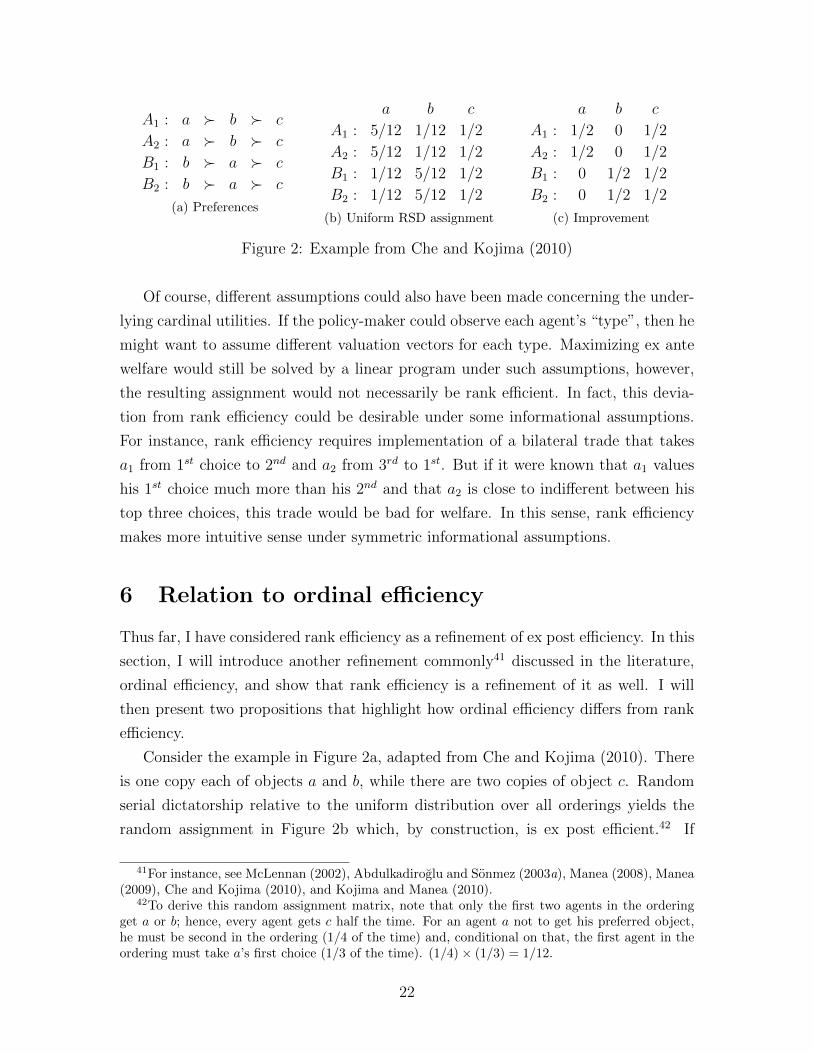
Figure 2: Example from Che and Kojima (2010)

Of course, different assumptions could also have been made concerning the under-

lying cardinal utilities. If the policy-maker could observe each agent’s “type”, then he

might want to assume different valuation vectors for each type. Maximizing ex ante

welfare would still be solved by a linear program under such assumptions, however,

the resulting assignment would not necessarily be rank efficient. In fact, this devia-

tion from rank efficiency could be desirable under some informational assumptions.

For instance, rank efficiency requires implementation of a bilateral trade that takes

a1 from 1st choice to 2nd and a2 from 3rd to 1st. But if it were known that a1 values

his 1st choice much more than his 2nd and that a2 is close to indifferent between his

top three choices, this trade would be bad for welfare. In this sense, rank efficiency

makes more intuitive sense under symmetric informational assumptions.

6 Relation to ordinal efficiency

Thus far, I have considered rank efficiency as a refinement of ex post efficiency. In this

section, I will introduce another refinement commonly41 discussed in the literature,

ordinal efficiency, and show that rank efficiency is a refinement of it as well. I will

then present two propositions that highlight how ordinal efficiency differs from rank

efficiency.

Consider the example in Figure 2a, adapted from Che and Kojima (2010). There

is one copy each of objects a and b, while there are two copies of object c. Random

serial dictatorship relative to the uniform distribution over all orderings yields the

random assignment in Figure 2b which, by construction, is ex post efficient.42 If

41For instance, see McLennan (2002), Abdulkadiroglu and Sonmez (2003a), Manea (2008), Manea(2009), Che and Kojima (2010), and Kojima and Manea (2010).

42To derive this random assignment matrix, note that only the first two agents in the orderingget a or b; hence, every agent gets c half the time. For an agent a not to get his preferred object,he must be second in the ordering (1/4 of the time) and, conditional on that, the first agent in theordering must take a’s first choice (1/3 of the time). (1/4)× (1/3) = 1/12.

22

each row of the assignment matrix represents a bundle of probability shares, however,

there is a mutually beneficial trade: A1 and A2 can trade their shares in b for the

shares of a held by B1 and B2, yielding the assignment in Figure 2c.43 Bogomolnaia

and Moulin (2001) first noticed this problem and suggested a refinement of ex post

efficiency which remedies it. Define the personal rank distribution of agent a

by Nx,a(k) ≡∑

o∈O 1ra(o)≤k · xao.

Definition 10. A feasible random assignment x ordinally dominates another as-

signment x if for all agents a, xa weakly stochastically dominates xa with respect to

%a, that is, N x,a(k) ≥ Nx,a(k) for all a ∈ A and k (strict for some a and k). An

assignment is called ordinally efficient if there is no other feasible assignment that

ordinally dominates it.

Bogomolnaia and Moulin (2001) showed that ordinal efficiency is a natural interim44

refinement of ex post efficiency, just as I earlier showed that rank efficiency can be

interpreted as an ex ante refinement of ex post efficiency. It is also true that rank

efficiency is a refinement of ordinal efficiency.

Proposition 6. If x is rank efficient, then x is ordinally efficient; however, the

converse need not hold.

Proof. The example from Figure 1a shows that the converse need not hold. For the

forward implication, note that weakly first-order stochastically improving all agents

(strict for one) will necessarily lead to a first-order stochastic improvement in the rank

distribution, since the global rank distribution is a sum over the agents’ individual

rank distributions.

Just as the random serial dictatorships always produce ex post efficient assign-

ments, the simultaneous eating mechanisms always yield ordinally efficient as-

signments (and can generate any ordinally efficient assignment). The formal descrip-

tion of this class of mechanisms is in Section C of the Appendix, but, essentially,

agents simultaneously claim object shares (“eat”) at an agent-specific, predefined

rate from their favorite (remaining) object, changing objects only when their current

43The Budish et al. (2011) extension of the Birkhoff-von Neumann theorem guarantees that thisnew assignment can also be resolved into a lottery over deterministic assignments. In fact, so longas the trades are one-for-one, this is true; the one-for-one requirement ensures that no agent endsup with shares that sum up to strictly more or less than one.

44Interim denotes the information set from which agent types are known, but the realized de-terministic assignment is not. In the context of assignment markets, this is the perspective whereagents’ ordinal preferences are known and the lottery over deterministic assignments has yet to beresolved.

23

favorite is exhausted.45 The probabilistic serial mechanism (PS) is the member

of this class where all agents “eat” at a uniform rate; it is the anonymous simultane-

ous eating mechanisms, just as uniform random serial dictatorship is the anonymous

random serial dictatorship. It is important to note that simultaneous eating mech-

anisms are generically non-strategy-proof and are absent in the field. Since ordinal

efficiency is such an attractive theoretical concept, it was unclear why there were no

ordinally efficient mechanisms in the field.46 The previous proposition, coupled with

the fact that rank efficient mechanisms do exist in the field resolves the puzzle. In-

stead of ordinal efficiency most broadly, institutional evolution seems to have chosen

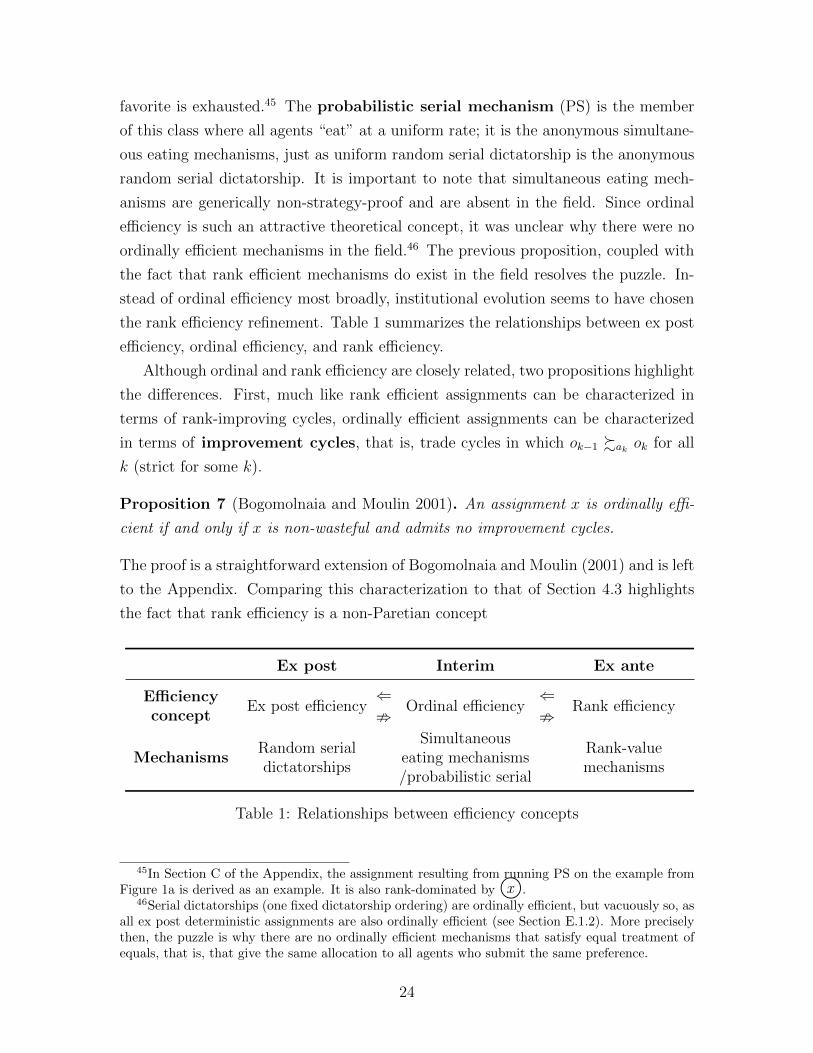
the rank efficiency refinement. Table 1 summarizes the relationships between ex post

efficiency, ordinal efficiency, and rank efficiency.

Although ordinal and rank efficiency are closely related, two propositions highlight

the differences. First, much like rank efficient assignments can be characterized in

terms of rank-improving cycles, ordinally efficient assignments can be characterized

in terms of improvement cycles, that is, trade cycles in which ok−1 %ak ok for all

k (strict for some k).

Proposition 7 (Bogomolnaia and Moulin 2001). An assignment x is ordinally effi-

cient if and only if x is non-wasteful and admits no improvement cycles.

The proof is a straightforward extension of Bogomolnaia and Moulin (2001) and is left

to the Appendix. Comparing this characterization to that of Section 4.3 highlights

the fact that rank efficiency is a non-Paretian concept

Ex post Interim Ex ante

Efficiencyconcept

Ex post efficiency⇐;

Ordinal efficiency⇐;

Rank efficiency

MechanismsRandom serialdictatorships

Simultaneouseating mechanisms/probabilistic serial

Rank-valuemechanisms

Table 1: Relationships between efficiency concepts

45In Section C of the Appendix, the assignment resulting from running PS on the example fromFigure 1a is derived as an example. It is also rank-dominated by x©.

46Serial dictatorships (one fixed dictatorship ordering) are ordinally efficient, but vacuously so, asall ex post deterministic assignments are also ordinally efficient (see Section E.1.2). More preciselythen, the puzzle is why there are no ordinally efficient mechanisms that satisfy equal treatment ofequals, that is, that give the same allocation to all agents who submit the same preference.

24

Second, conditional on an assignment being deterministic, ordinal efficiency is

equivalent to ex post efficiency, while rank efficiency remains a refinement. Formally,

Proposition 8. Let x be a deterministic assignment. Then,

(i) x is ordinally efficient if and only if it is ex post efficient.

(ii) x is rank efficient implies it is ex post efficient; however the converse need not

hold.

Motivating rank efficiency as ex ante efficiency, modulo a few assumptions, is theoret-

ically pleasing, but policy-makers tend to think in terms of deterministic assignments.

If this is true, then the preceding distinction might shed some light on why simultane-

ous eating mechanisms aren’t seen in the field. Rank efficiency is a strict refinement

even when only deterministic assignments are being compared.

7 The potential gains of the rank-value mechanism

As mentioned previously, both the ordinally efficient and rank efficient mechanisms

are generically non-strategy-proof. This could be a major problem, as agent manip-

ulation of reported preferences could yield assignments that look good relative to

the submitted preferences, but are quite bad relative to the true preferences. In this

section, I consider a simple empirical exercise that sheds light on this risk. Running

uniform random serial dictatorship (the baseline strategy-proof mechanism) gives an

idea of how efficient a match can be without sacrificing strategy-proofness. The pref-

erences submitted to a strategy-proof mechanisms should be truthful, so to get an

idea of the potential for gains, I can take those preferences and use them to run a non-

strategy-proof alternative, such as the probabilistic serial mechanism or a rank-value

mechanism. The efficiency of these counterfactuals is a sort of best-case analysis:

if there is not significant improvement even without manipulation, then sacrificing

strategy-proofness is likely not worth considering.

7.1 Assigning students to overseas programs at Harvard Busi-

ness School

At Harvard Business School (HBS), first year MBAs must participate in a global

immersion program.47 They are assigned to a foreign company and remotely work

47At HBS, it is known as the FIELD 2 program.

25

on a project with that company during the first semester. The program culminates

in a two-week trip over the winter break in which the MBA will present her work in

person and be given the opportunity to make foreign business contacts.

In 2011, at the beginning of their first semester at HBS, 900 MBAs were asked

to rank the 11 different countries to which they could be assigned.48 The mechanism

we49 used to match the students was strategy-proof, so the preferences submitted to

it can be taken as truthful. Note that we allowed the MBAs to express indifferences;

the strategy-proof adaptation of random serial dictatorship that we used is briefly

described in the Appendix. In the interests of simplicity, however, I randomly broke

student indifferences and considered only strict preference assignment mechanisms.

All results are qualitatively the same regardless of the method used to break student

indifferences, and regardless of whether indifferences are broken. Results from these

alternate specifications are included in the Appendix.

7.2 The data

The data used for the analysis in this section is borrowed from Featherstone and

Roth (2011). Figure 3 shows the rank distributions yielded by uniform random serial

dictatorship, probabilistic serial (note that these first two overlap on the graph), and

the v-rank-value mechanism, where the valuation vector50 is

v = (100, 80, 50, 35, 15, 10, 5, 3, 2, 1, 0.5)

The first thing to notice is that the rank distribution from probabilistic serial is

essentially identical to that of uniform random serial dictatorship. The underlying

assignments are also very similar, which means that, in the HBS context, there is

little reason to favor the more complicated probabilistic serial mechanism over the

simpler uniform random serial dictatorship. Che and Kojima (2010) show that, the-

oretically, the random assignment generated by the probabilistic serial mechanism

asymptotically converges to the random assignment generated by uniform random

serial dictatorship in the large market limit. Often with asymptotics, however, it is

hard to know how large is large enough. In the case of HBS, 900 students and 11

48Students only rank countries; once they are assigned to a country, the company they get isadministratively assigned without their input.

49I designed the HBS match jointly with Al Roth.50Other valuation vectors yield similar results; the main purpose I document the specific valuation

used is to assure the reader that the analysis in this section doesn’t depend on a particularly extremechoice of v.

26

countries seems sufficient.

Perhaps more striking is how well the v-rank-value mechanism performs. The

number of students who get their first or second choice is increased by more than

15% when we move from the uniform random serial dictatorship to the rank-value

mechanism. This corresponds to about 120 students. So, the gains from moving

to a rank-value mechanism might indeed be large enough to justify backing away

from strategy-proofness. However, these figures come from a best-case analysis. It

could be that manipulation completely undermines the gains, or even makes the rank-

value mechanism perform worse than random serial dictatorship.51 The analysis of

this section simply makes the case that backing away from strategy-proofness for the

gains given by probabilistic serial does not make sense for the HBS match, but that

doing so for the gains given by the rank-value mechanism might well be worthwhile.

7.3 Strategy-proofness versus improved efficiency

The previous exercise illustrates that the concept of rank efficiency and its asso-

ciated rank-value mechanisms fit well with previous literature that has considered

the costs of strategy-proofness in stable matching (Erdil and Ergin 2008, Abdulka-

diroglu, Pathak and Roth 2009, Azevedo and Leshno 2010). Papers on the costs of

strategy-proofness in non-stable assignment have mostly focused on how the Boston

mechanism (Abdulkadiroglu and Sonmez 2003b) can outperform random serial dicta-

torship. Featherstone and Niederle (2011) show this in the context of a truth-telling

equilibrium, while Abdulkadiroglu, Che and Yasuda (2011) focus on a non-truth-

telling equilibrium. Both papers rely on stylized assumptions about how preferences

are distributed. The present paper differs in two ways. First, it offers a new approach

to get at cardinal utility in the context of an ordinal mechanism: make reasonable

assumptions and maximize welfare accordingly. Second, in past literature, the leading

contender with random serial dictatorship has been the class of Boston mechanisms.

This paper offers a new mechanism that is based on the well-established empirical

fact that policy-makers care about rank distributions.52,53 As I have begun to show in

51Note that the work we do in Section 8 indicates that in at least some environments, we expecttruth-telling.

52Note that the Boston mechanism is not entirely ad hoc: it has been axiomatized by Kojimaand Unver (2011).

53Also, notice that the Boston mechanism is not a v-rank-value mechanism for any v. To see this,consider the example of Figure 1a. The Boston mechanism would give object a to 1 half the time, andto 2 the other half of the time. But, Claim 2 shows that this is not a rank efficient assignment, andTheorem 1 shows that rank-value mechanisms must yield rank efficient assignments. The Bostonmechanism is not forward-looking (i.e. it is a greedy algorithm), which is a requirement for any

27

60%

65%

70%

75%

80%

85%

90%

95%

100%

1 2 3 4 5 6 7 8 9 10 11

Ran

ked

kth

or

bet

ter

k

U-RSD

PS

RVM

Figure 3: Rank distributions for our mechanisms(U-RSD is Uniform Random Serial Dictatorship, PS is Probabilistic Serial, and RVM is Rank-Value

Mechanism. Note that U-RSD and PS overlap.)

28

this section, the rank-value mechanisms might be an important part of the discussion

about the costs of strategy-proofness in ordinal assignment markets.

8 Incentives for truth-telling

I begin this section by showing that efficiency and strategy-proofness are theoretically

incompatible. There are two ways that rank-value mechanisms could still work in light

of this. First, there could be environments in which rank-value mechanisms admit

manipulating equilibria in which the efficiency gains don’t disappear, much like in

Abdulkadiroglu, Che and Yasuda (2011). Second, there could be environments in

which truth-telling can be supported in equilibrium. Although, the first possibility is

interesting, in this paper, I will focus on the second.

8.1 An impossibility result

A mechanism is called strategy-proof if the allocation it gives to any agent when

she truthfully reveals her ordinal preference stochastically dominates the allocation it

would give her if she revealed anything else. A mechanism is called weakly strategy-

proof if the allocation it gives to an agent when she deviates from truth-telling never

strictly stochastically dominates what it gives her when she truthfully reveals. An-

other way to phrase the difference between these two concepts is in terms of the car-

dinal preferences that rationalize the true ordinal preferences. Strategy-proof means

that truth-telling is a dominant strategy regardless of the rationalizing cardinal util-

ities. Weakly strategy-proof means that for any beliefs and any potential lie, there

exist rationalizing cardinal utilities that make truth-telling a better-response.

Theorem 3. No rank efficient mechanism is strategy-proof. In fact, no rank efficient

mechanism is even weakly strategy-proof.

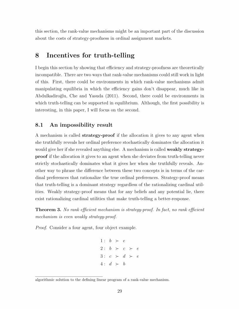
Proof. Consider a four agent, four object example.

1 : b e

2 : b c e

3 : c d e

4 : d b

algorithmic solution to the defining linear program of a rank-value mechanism.

29

The unique54 rank efficient allocation is (1, e) , (2, b) , (3, c) , (4, d). So under any

rank efficient mechanism, 1 must be assigned to e. Now, consider what happens if

1 deviates from truth-telling and submits b c d e instead. Now, the unique

rank efficient allocation is (1, b) , (2, e) , (3, c) , (4, d). Hence, under any rank efficient

mechanism, 1 gets b with the deviation, which first-order stochastically dominates the

certain e he would get with the truth.

Intuitively, someone has to get stuck with e. Under the true preferences, the

mechanism pays the smallest price for assigning e to Agent 1. When he submits

b c d e instead, he is exaggerating about how bad e is for him, making it

better for the mechanism to give it to Agent 2 instead. Still, this example required

quite a bit of specific knowledge. Next, I will show that truth-telling is a natural

response in some environments where agents have much less information.

8.2 A possibility result

Following Roth and Rothblum (1999), for some preference profile %, define %o↔o′ to

be the same preference profile, except all agents have switched the objects o and o′

in their ordinal rankings. Define qo↔o′

to switch the capacities of o and o′, and let

xo↔o′

denote the (possibly infeasible) assignment where everyone assigned to o in x

is reassigned to o′ and vice-versa. Finally, define the action of the o ↔ o′ operator

on the tiebreaker by τ(x)o↔o′ ≡ τ

(xo↔o

′). Note that xo↔o

′will be feasible if the

capacities are switched to qo↔o′. An agent a’s beliefs are then summarized by a

vector of random variables that range over potential ordinal preferences of the other

agents (%−a%−a%−a), capacities of the objects (qqq), and tie-breaker numberings, (τττ). We treat

%a, A, and O as known.

Definition 11. An agent’s beliefs are o, o′-symmetric if the distributions of

(%−a%−a%−a, qqq, τττ) and (%−a%−a%−a, qqq, τττ)o↔o′

coincide. If the beliefs are o, o′-symmetric for all

o, o′ ∈ O \ ∅, then we simply call the beliefs symmetric.

One interpretation of this condition is that it represents a very symmetric envi-

ronment. The interpretation I favor, however, is that it represents an environment in

which agents have very little specific information, that is, an environment in which,

to the agents, nothing really distinguishes one object from the other. Even when this

is not globally true, it is often the case that preferences are tiered and that, within a

54For an example of how to show that an assignment is the unique rank efficient assignment, seeClaim 2 above.

30

tier, beliefs are close to symmetric. Note that this condition is well defined even for

preferences that have indifferences. Under this informational assumption, switching

the order of two objects in the submitted preference is not profitable. Formally,

Proposition 9. Under a rank-value mechanism, if agent a’s beliefs are o, o′-symmetric,

and o′ a o, then for a, the allocation resulting from any submitted preference that

declares o a o′ is weakly stochastically dominated by the allocation resulting from a

submitted preference that does not. If the beliefs are symmetric, then this holds for

all o, o′ ∈ O \ ∅.

The proof for the theorem leverages the symmetry assumption to show that for

every state of the world in which the lie is profitable, there is at least one equally

likely state of the world in which it is not. This result is stated in a way that allows

for indifference, but from this point on in the main text, for expositional ease, I will

only consider assignment markets where all preferences are strict. For the interested

reader, the more general results for indifferences are in the Appendix. An immediate

corollary of Proposition 9 is that if an agent has strict preferences and must rank all

objects, then he does best to truth-tell if his beliefs are symmetric. Formally,

Theorem 4. Under a rank-value mechanism, if an agent’s beliefs are symmetric, his

preferences are strict, and he is required to rank all objects, then the allocation he

receives under truth-telling weakly stochastically dominates the allocation he receives

under any other strategy.

Corollary to Theorem 4. Under the conditions of Theorem 4, all agents truth-

telling is an equilibrium.

Although the requirement to rank all objects may seem unrealistic, it is actually

quite prevalent in the field. Consider public school assignment. Students are not

required to rank all schools, but if they cannot be assigned to a school they ranked,

they are generally given an administrative assignment.55 In this sort of situation,

failing to rank all schools is equivalent to the student saying to the school district,

“beyond what I ranked, you can fill out the rest of my rank-order list for me.” As

an aside, Teach for America also does not allow agents to rank the null object: any

admit will get some assignment with their offer of admission.

55I know that this is the policy in the San Francisco Unified School District because I and co-authors (Atila Abdulkadiroglu, Muriel Niederle, Parag Pathak, and Al Roth) spent a year redesigningthe assignment system; however, it is hard to imagine a school district that doesn’t work in thisway, as all students legally must be able to claim some seat in a public school, even after the matchhas run.

31

8.3 Characterizing exhaustive manipulation classes

Nevertheless, one might feel that forcing agents to rank all objects is too onerous

an assumption. If I relax this requirement, I can still tightly characterize classes

of manipulations with which an agent can always best respond. The surprise of

this exercise is that it hinges on an otherwise unremarkable detail of the design.

Implementing mechanisms in the field often focuses attention on things that might

otherwise be assumed away, and the results in this section are a result of carefully

considering what a rank-value mechanism should look like in the context of the HBS

global immersion match discussed in Section 7. How the null object is treated in the

rank scheme turns out to be of great import.

To understand manipulation when agents are not required to rank all objects, I

must first resolve the ambiguity concerning rank functions mentioned near the end of

Section 2. First, define a rank scheme to be upward-looking if ra(o) is independent

of the preferences among objects to which o is strictly preferred . Now, consider how

to deal with the outcome of being unmatched in the case of an agent whose true

preferences are a b ∅. One natural alternative is to treat ∅ like any other object,

that is r(a) = 1, r(b) = 2, and r(∅) = 3. Often, however, policy-makers think of

being unmatched as a distinct worst element in the overall rank distribution;56 that

is, r(∅) = |O|, regardless of how many objects the agent declared acceptable. To help

in thinking about this, consider inserting a new indifference class, I, which contains

only o, below all acceptable objects in %a (but ahead of ∅). Call this new preference

%+Ia . If r%+I

a(o) = r%a(∅), then call the ranking scheme unmatched-neutral, as ∅ is

treated just as any other object. If r%+Ia

(∅) = r%a(∅), then call the ranking scheme

unmatched-distinct. In this language, the example where ∅ is treated just like

any other object is unmatched-neutral, and the example where ∅ is always given the

lowest rank possible is unmatched-distinct.

Now, I define two important classes of manipulations. Call a submitted preference

%′a a truncation of the true preference %a if there is some object o %a ∅ such that

%o↔∅a is equivalent57 to %′a above ∅. Similarly, call a submitted preference %′a an

extension of the true preference %a if there is some object ∅ %a o such that %o↔∅a is

equivalent to %′a. Under these definitions, truth-telling is both a truncation and an

extension (when o = ∅).

Theorem 5. If an agent’s beliefs are symmetric, his preferences are strict, and the

56See Footnote 17.57In the rank-value mechanism, how things are listed below ∅ does not matter because ∅ is never

scarce.

32

rank scheme is upward-looking and...

• ...unmatched-distinct, then his allocation from any other strategy is weakly stochas-

tically dominated by his allocation from playing some truncation.

• ...unmatched-neutral, then his allocation from any other strategy is weakly stochas-

tically dominated by his allocation from playing some extension.

Note that I can’t leverage both parts of the theorem simultaneously to find a condition

for truth-telling.

Claim 7. A ranking scheme cannot be both unmatched-neutral and unmatched-

distinct.

Proof. If it is unmatched-neutral, then r%+Ia

(o) = r%a(∅), which means that r%+Ia

(∅) >r%a(∅), contradicting the assumption that the ranking scheme was unmatched-distinct.

Truncations are a familiar class of strategies,58 and the intuition for why they can

be profitable is simple. When the ranking scheme is unmatched-distinct, a truncation

can be interpreted as an agent threatening the linear program: “give me something

I like, or pay the price of giving me ∅”. When the ranking scheme is unmatched-

neutral, this threat no longer works, as truncating actually relaxes the optimization.

So why extensions? Intuitively, consider an agent whose preference is a b ∅ in a

market with 100 other agents whose preferences are a b c d e f ∅. If

the agent doesn’t extend, the linear program will assign him to ∅, since doing so is

worth v3 − v7 more than the alternative of putting some other agent in ∅.So even in low information environments, agents can gain, but it is notable that

they gain by using a class of strategies very similar to those that can theoretically

be used to game two-sided deferred acceptance in a low information environment. In

the lab, Featherstone and Mayefsky (2011) show that subjects can fail to truncate

under a deferred acceptance mechanism, leaving a significant amount of money on the

table by doing so. It would be interesting to see if a similar result held for rank-value

mechanisms,59 and in fact, the experimental and computational work of Unver (2001)

58The paper in which our informational assumption was first used, Roth and Rothblum (1999),found that, in symmetric environments, agents on the proposed-to side of a deferred acceptancemechanism can always do just as well with a truncation.

59The theorems just proved can help in the design of experiments that deal with the large strat-egy space of ordinal mechanisms, by allowing the experimenter to focus only on truncations orextensions. For a taste of how this might work, see Featherstone and Mayefsky (2011), which usesthe “truncations are exhaustive” result of Roth and Rothblum (1999) to yield a more analyticallytractable design.

33

and Unver (2005) indicate that this is a real possibility.

9 Connection to competitive equilibrium mecha-

nisms

In order to talk about the fairness properties of rank-value mechanisms, I must first

generalize rank efficiency by allowing agents to be weighted differently in the rank

distribution. In doing so, I will show that some ordinally efficient assignments are

not rank efficient relative to any weights. This generalization is also of independent

interest because it strongly relates to an ordinal adaptation of the much-discussed

pseudomarket mechanism of Hylland and Zeckhauser (1979), in which agents are

given a budget of artificial money and a competitive equilibrium is computed.

9.1 Generalizing rank efficiency

Until now, all agents have been equally weighted in the rank distribution, which

is equivalent to saying that the utility an agent gets from a kth choice is directly

comparable to the utility any other agent gets from a kth choice.60 I will weaken

this assumption by allowing for a general weighting scheme in the rank distribution.

Define the rank distribution of assignment x with respect to weights ααα (or

the α-rank distribution for short) to be

Nxα(k) ≡

∑a∈A

∑o∈O

αa · 1ra(o)≤k · xao

Nxα(k) is the weighted expected number of agents who get their kth choice or better

under assignment x.

Definition 12. A feasible random assignment x is ααα-rank dominated by another

feasible assignment x if the α-rank distribution of x first-order stochastically dom-

inates that of x, that is, N xα(k) ≥ Nx

α(k) for all k (strict for some k). A random

assignment is called ααα-rank efficient if it is not α-rank-dominated by any other

feasible assignment.

The mechanisms that correspond to α-rank efficiency are a similarly modified

version of the v-rank-value mechanisms.

60The interpersonal utility comparison is actually more subtle than this; see Section 5.2 for adiscussion.

34

Definition 13. The rank-value mechanism with respect to weights α and

valuation v (or the (α,v)-rank-value mechanism for short) maps agent rank

orderings to a maximizer of the following linear program.

maxx

∑a∈A

∑o∈O

αa · vra(o) · xao

s.t.∑a

xao ≤ qo, ∀o ∈ O∑o

xao ≤ 1 , ∀a ∈ A

xao ≥ 0 ,∀o

∀a

∈ O

∈ A

We say that the assignments in the arg max are supported by the (α,v)-rank-

value mechanism.

Everything proven thus far can be easily adapted to the generalization; proofs in the

appendix are done with respect to a non-specific α.

9.2 Supportable rank efficiency

Of course, one might not want to make any assumption about how agents’ utilities

compare. The following concept makes this idea precise.

Definition 14. An assignment x is called supportably rank efficient if there exists

an α such that x is α-rank efficient.

Supportable rank efficiency implies ordinal efficiency;61 however, it is perhaps sur-

prising that ordinally efficient assignments can fail to be supportably rank efficient.

Theorem 6. Supportable rank efficiency implies ordinal efficiency. The converse

need not hold.

The intuition behind the negative statement is rooted in appropriate generalization

of the “tough decisions” trade cycles of Section E.1.2. For an assignment to be

supportably rank efficient, there must be one (α, v) pair such that all trade cycles

fail to be (α, v)-rank improving.62 For every trade cycle then, there is a (possibly

61Supportable rank efficiency implies α-rank efficiency (for some α) which, by the easy general-ization of Proposition 6, implies ordinal efficiency.

62In Definition 9, replace∑k

[vrak

(ok−1) − vrak(ok)

]> 0 with

∑k

αak·[vrak

(ok−1) − vrak(ok)

]> 0.

35

empty) region of (α, v) space such that it is not (α, v)-rank improving. This region

can be characterized by a simple inequality. The proof of the theorem starts with an

ordinally efficient assignment and then defines trade cycles until the corresponding set

of inequalities has no solution. There is nothing special about the counterexample;

as an assignment grows large, it has many trade cycles, so unless special provision

is made to keep them all from being (α, v)-rank improving relative to some common

(α, v), it is no surprise that the system of inequalities cannot be satisfied. The proof

suggests a natural conjecture (which I do not prove in this paper): as the market

grows, the size of the set of supportably rank efficient assignments becomes small

when compared to the size of the set of ordinally efficient assignments. Also, note

that there is no reason that probabilistic serial assignments are special; in fact, the

proof to Theorem 6 uses a probabilistic serial assignment to get the ordinally efficient

assignment that forms the counterexample.

Corollary to the proof. Probabilistic serial does not always yield supportably rank

efficient assignments.

This result might seem especially surprising in the light of McLennan (2002) and

Manea (2008), who both find (using non-constructive and constructive methods, re-

spectively) that any ordinally efficient assignment is ex ante efficient relative to some

set of cardinal preferences that rationalize the ordinal preferences. The difference here

is that, as shown in Section 5.2, the concept of rank-efficiency imposes the added con-

straint that all agents must share the same cardinal utility (in expectation) across

ranks.

9.3 Competitive equilibrium mechanisms

An assignment is supportably rank efficient if and only if it can be supported by the

(α, v)-rank-value mechanism for some (α, v). This is a straightforward corollary of

the Generalization of Theorem 1 proved in Section E.1.1 of the Appendix. It is also

true, however, that an assignment is supportably rank efficient if and only if it can

be generated by a certain adaptation of the pseudomarket mechanisms of Hylland

and Zeckhauser (1979). The idea of these mechanisms is to 1) use a valuation vector

to convert agents’ ordinal preferences to cardinal preferences, 2) give each agent a

budget of artificial money, and 3) calculate a competitive equilibrium in the market

where goods are probability shares in the objects. Formally,

Definition 15. The prices and random assignment (x, p), form a budget equilib-

36

rium with respect to valuation vvv and budgets B if, for all a,

xa ∈ arg maxxa≥0

∑o

vra(o) · xao

s.t.∑o

po · xao ≤ Ba∑o

xao ≤ 1

and

xao ∈ arg maxxao≥0

∑a

∑o

po · xao

s.t.∑a

xao ≤ qo ,∀o

A (B,v)-budget mechanism maps ordinal preferences to an assignment that is

part of a (B, v)-budget equilibrium, and the assignment is said to be supported by

the (B, v)-budget mechanism.

The first optimization can be thought of as the agent’s problem, and the second as

the producer’s problem. Note that calculating a budget equilibrium is more difficult

than solving the rank-value linear program.63

Remark 7. The producer’s problem is equivalent to∑a

xao ≤ qo and po > 0⇒∑a

xao =

qo, for all o ∈ O.

The resemblance64 of budget equilibria to the more familiar competitive equilib-

rium suggests that there should also be results resembling the first and second welfare

theorems. Supportable rank efficiency is the efficiency concept needed to complete

the analogy. Formally,

Theorem 7. x is supportably rank efficient if and only if there exist budgets and a

valuation, (B, v), such that x is supported by the (B, v)-budget mechanism.

The intuition for this proof comes from considering the linear programming du-

als of the optimizations involved in the (α, v)-rank-value mechanism and the (B, v)-

budget mechanism. If x is a supportably rank efficient assignment, then it must be

63Budget equilibria can be approximately solved using a method laid out in the appendix ofHylland and Zeckhauser (1979), which in turn grapples with the known-to-be-difficult problem ofapproximating Kakutani fixed points (Scarf 1967, Scarf and Hansen 1973, Chen and Deng 2008).Polynomial time methods are known for markets in which agents are not limited by the

∑o xao ≤ 1

constraint (Nisan 2007), but it is unclear whether such results can be generalized to budget equilibria.64Note that the (α, v)-rank-value mechanism can be decentralized to look like a competitive

equilibrium as well. This decentralization, which I call an (α, v)(α, v)(α, v)-discount equilibrium is definedand characterized in Section E.4 of the Appendix.

37

in the arg max of the (α, v)-rank-value mechanism for some (α, v). Keeping the same

valuation v for the budget equilibrium, the shadow prices associated with the object

quota constraints will decentralize x, so long as each agent a can afford his allocation,

xa, which can be guaranteed by giving him a budget Ba =∑

o po ·xao. For the reverse

implication, start with an assignment x that is a (B, v)-budget equilibrium, keep the

same valuation, and set αa equal to the inverse of the budget shadow price in agent

a’s optimization.65

An important corollary to the proof of this proposition is that, for a given val-

uation v and set of preferences %, there is a natural mapping between weights α

and budgets B. Although not immediately obvious, the proof also shows that as-

signments in the arg max of the procedurally fair (all agents are weighted the same)

v-rank-value mechanism are supported by a budget equilibrium that is not procedu-

rally fair (budgets are not guaranteed to be equal). Similarly, budget equilibrium from

equal budgets gives assignments that are supported by an (α, v)-rank-value mecha-

nism in which the weights are not guaranteed to be equal. In this sense, procedural

fairness is fundamentally different between rank-value mechanisms and budget mech-

anisms. In the next section, I will show how this tension sheds light on the theoretical

incompatibility of rank efficiency and envy-freeness.

10 Justice and rank-efficiency

Looking at the example from Figure 1a, one might object that Agent 1 has been

unfairly singled out. Envy-freeness is the idea that makes this intuition precise. Let an

assignment be strongly envy-free if xa weakly first-order stochastically dominates

xa′ relative to %a, for all a, a′ ∈ A. Let an assignment be weakly envy-free if

there is no a′ ∈ A such that xa′ strongly first-order stochastically dominates xa

relative to %a, for all a ∈ A. Finally, let an assignment be envy-free relative to

some cardinal preferences if each agent weakly prefers his own allocation to all other

agents’ allocations.

Theorem 8. No mechanism is rank efficient and even weakly envy-free

Proof. Consider the example from Figure 1a. x© is the unique rank efficient as-

signment, so any rank efficient mechanism must choose it. But 1 would prefer 2’s

65Extra care must be taken when the shadow price is zero. This case is worked out in more detailin the Appendix.

38

allocation, regardless of the cardinal preferences that rationalize his ordinal prefer-

ence.

This theorem implicitly deals with two philosophical concepts of justice. Dworkin

argues for the dual requirements of ex post efficiency and envy-freeness, which he calls

“equality of resources” (Dworkin 1981).66 Harsanyi, in contrast, argues for policy to

be chosen as if by an expected utility maximizer in the Rawlsian67 original posi-

tion68, a concept which I will call “Harsanyian justice” (Harsanyi 1975). In terms

of these concepts, Theorem 8 says that in assignment markets, equality of resources

and Harsanyian justice cannot be jointly guaranteed. This is no surprise in view of

the proof of Theorem 7. An assignment implemented by a budget equilibrium from

equal budgets is, in some sense, envy-free, since all agents have the same opportu-

nity set. But this same assignment might also be implementable by a rank-value

mechanism with unequal weights, contradicting Harsanyian justice. To move forward

from Theorem 8 then, one must make a choice. As discussed in Section 5.2, the

rank-value mechanism with equal weights guarantees Harsanyian justice (modulo a

few assumptions). But how does one guarantee equality of resources?

Proposition 10. If there exist prices p, a valuation v, and budgets B, such that

Ba = Ba′ for all a, a′ ∈ A and (x, p) is a (B, v)-budget equilibrium, then x is weakly

envy-free and supportably rank efficient. Further, x is envy-free relative to the cardinal

preferences encoded by v.

Proof. Theorem 7 established that budget equilibria are supportably rank efficient.

Now, assume that xa′ strongly first-order stochastically dominates xa relative to %a.

Then, for any v, agent a’s objective in the definition of the (B, v)-budget equilibrium

must be higher at xa′ than at xa. But a could have afforded xa′ by the equal budgets

assumption. This contradicts optimality. Envy-freeness relative to v follows by similar

logic.

So, budget equilibrium from equal budgets yields weak envy-freeness and sup-

portable rank efficiency (which implies ex post efficiency). Although this provides a

66In fact, Dworkin (1981) literally suggests a cardinal version of this paper’s budget equilibriumfrom equal budgets as an embodiment of the idea.

67Although Harsanyi’s conception of justice is based on Rawls’ veil-of-ignorance, the DifferencePrinciple (i.e. insistence on a maximin objective from the original position) places Rawls’ conceptionmore in line with Dworkin’s (Rawls 1972).

68That is, from the perspective of a fictional agent who knows that they will become one ofthe agents in the market, uniformly and at random, and will inherit that agent’s preferences andallocation.

39

partial workaround to the impasse of Theorem 8, weak envy-freeness is not a strong

condition: it only guarantees that there exist rationalizing cardinal utilities that make

the assignment envy-free. Still, the exercise is very similar to how the v-rank-value

mechanism can be justified as maximizing social welfare: in the absence of cardinal

information, make assumptions and push forward. Under such assumptions, budget

equilibrium from equal budgets yields an envy-free assignment. Finally, note that the

probabilistic serial mechanism of Bogomolnaia and Moulin (2001) is strongly envy

free, but as shown in Section 9.2, it may not be ex ante efficient in a world where

beliefs about agents’ cardinal preferences meet the conditions of Proposition 5.69

11 Conclusion

Rank efficiency is a natural concept that is used in the field, and under truth-telling,

rank efficient mechanisms can yield significant welfare gains. Unfortunately, rank

efficiency is also theoretically incompatible with strategy-proofness. This does not

mean, however, that the market designer should freely dismiss it. In the words of

Day and Milgrom (2008),

“...it is customary in mechanism design theory to impose incentive con-

straints first, investigating other aspects of performance only later. It

is, of course, equally valid to begin with other constraints and such an

approach can be useful. To the extent that optimization is only an ap-

proximation to the correct behavioral theory for [agents], it is interesting

to investigate how closely incentive constraints can be approximated when

other constraints are imposed first.”

The situation in this paper is not unique: there is a growing body of literature that

points to the fact that the costs of strategy-proofness can be quite high. So, when

then should the market designer pay this cost? In this paper, I show that truth-telling

is an equilibrium of rank-value mechanism in a stylized, low-information environment.

Such a theorem highlights the important intuition that rank-value mechanisms are

more likely to work when agents know little about the popularity of the objects.

Even so, it seems likely that there exist environments in which the performance

of rank efficient mechanisms will be unacceptably poor. Unfortunately, any such

69Note that the wedge between fairness and efficiency exists in the cardinal setting as well.Competitive equilibrium from equal incomes (Varian 1974, Hylland and Zeckhauser 1979) givesPareto efficiency, but Negishi’s theorem (Negishi 1960) does not guarantee that the correspondingweights in the planner’s problem will be equal.

40

characterization is again likely to be limited to a stylized model, and characterizations

that truly generalize across environments seem intractable. In addition, it is certainly

plausible that in more complicated situations, equilibrium predictions will be not

be born out in the field (see Featherstone and Niederle (2011) and Featherstone

and Mayefsky (2011)). Thus, to understand when the costs of strategy-proofness

are too dear, theoretical results will need to be complemented with more empirical

approaches, such as experiments and learning models.

Regardless of such evidence however, it may be that in the long run, in any

environment in which a mechanism fails to admit a truth-telling equilibrium, agents

will eventually converge to a manipulating equilibrium. Even if this is true, it might

still be worthwhile to consider how much the short run can be extended. Consider the

HBS match discussed in Section 7. In the first year of the match, had we run a rank

efficient mechanism, it is quite plausible that agents would have truthfully revealed

their preferences. We didn’t do this, however, because we were worried about the

MBAs learning to manipulate over time. Taking extra efficiency in the first year,

at the expense of subsequent years, seemed like too much of a “smash-and-grab”

strategy. But what if the learning process were slower, such that the efficiency gains

could be reaped for the first five years? In such a setting, the “smash-and-grab”

strategy starts to sound like a good idea; in fact, one could even imagine running

a rank efficient mechanism for four years and then switching to a strategy-proof

mechanism as learning began to cause problems. Thinking about ways to slow the

speed with which agents learn to manipulate a non-strategy-proof mechanism seems

like an interesting, and thus far, unpursued line of research. When the efficiency cost

of strategy-proofness is high, as I have shown can be the case, this line of inquiry

could prove quite fruitful.

While there are many papers on the costs of strategy-proofness in matching mech-

anisms, the costs of Pareto-agnosticism have not been as carefully considered. In this

paper, I show that if the policy-maker truly considers all kth choice assignments as

interchangeable, then by allowing him to express this, the rank-value mechanism can

yield big welfare gains. For more complicated welfare considerations, the (α, v)-rank

efficient mechanisms or the generalizations of rank-value mechanisms mentioned at

the end of Section 5.2 could help. The lessons from the mechanisms in this paper are

then twofold. First, although economists are not in a position to make ethical judge-

ments about interpersonal utility comparison, policy-makers are. It makes sense then

for market designers to use mechanisms that have a place for policy-maker’s judge-

ments to be inputted, like the α in the (α, v)-rank-value mechanisms. Second, armed

41

with the power to make such judgements, market designers can significantly improve

welfare.

The fact that there are rank efficient mechanisms in the field could mean that

they are successful in some situations. Alternatively though, it might be that well-

intentioned policy-makers, ignorant of incentive concerns, are implementing bad poli-

cies. Market designers need to know whether they should be correcting the impulse

to depart from strategy-proofness or sometimes suggesting that it is a small price to

pay for potentially big welfare gains. Which advice is good very likely depends on the

environment in which the mechanism is meant to serve and on the dynamics of the so-

cial learning process. Understanding when (if ever) market designers can comfortably

suggest a rank efficient mechanism seems like an important open question.

42

References

Abdulkadiroglu, Atila, and Tayfun Sonmez. 1998. “Random serial dictatorshipand the core from random endowments in house allocation problems.” Economet-rica, 689–701.

Abdulkadiroglu, Atila, and Tayfun Sonmez. 2003a. “Ordinal efficiency anddominated sets of assignments.” Journal of Economic Theory, 112(1): 157–172.

Abdulkadiroglu, Atila, and Tayfun Sonmez. 2003b. “School choice: A mecha-nism design approach.” The American Economic Review, 93(3): 729–747.

Abdulkadiroglu, Atila, Parag Pathak, and Alvin E. Roth. 2009. “Strategy-proofness versus Efficiency in Matching with Indifferences: Redesigning the NewYork City High School Match.”

Abdulkadiroglu, Atila, Yeon-Koo Che, and Yosuke Yasuda. 2011. “Resolvingconflicting preferences in school choice: The Boston mechanism reconsidered.” TheAmerican Economic Review, 101(1): 399–410.

Azevedo, Eduardo M., and Jacob Leshno. 2010. “Can We Make School ChoiceMore Effiicient?” unpublished mimeo.

Berge, Claude. 1957. “Two theorems in graph theory.” Proceedings of the NationalAcademy of Sciences of the United States of America, 43(9): 842.

Birkhoff, Garrett. 1946. “Tres observaciones sobre el algebra lineal.” Univ. Nac.Tucuman Rev. Ser. A, 5: 147–151.

Bogomolnaia, Anna, and Herve Moulin. 2001. “A new solution to the randomassignment problem.” Journal of Economic Theory, 100(2): 295–328.

Bogomolnaia, Anna, Rajat Deb, and Lars Ehlers. 2005. “Strategy-proof assign-ment on the full preference domain.” Journal of Economic Theory, 123(2): 161–186.

Budish, Eric. 2009. “The combinatorial assignment problem: Approximate com-petitive equilibrium from equal incomes.” University of Chicago, Booth School ofBusiness, Unpublished mimeo.

Budish, Eric, and Estelle Cantillon. forthcoming. “The Multi-unit AssignmentProblem: Theory and Evidence from Course Allocation at Harvard.” The AmericanEconomic Review.

Budish, Eric, Yeon-Koo Che, Fuhito Kojima, and Paul Milgrom. 2011.“Implementing Random Assignments: A Generalization of the Birkhoff-von Neu-mann Theorem.” University of Chicago, Columbia University, Stanford University,unpublished mimeo.

Burkard, Rainer E., Mauro Dell’Amico, and Silvano Martello. 2009. Assign-ment problems. Society for Industrial Mathematics.

43

Chen, Xi, and Xiaotie Deng. 2008. “Matching algorithmic bounds for finding aBrouwer fixed point.” J. ACM, 55: 13:1–13:26.

Che, Yeon-Koo, and Fuhito Kojima. 2010. “Asymptotic equivalence of proba-bilistic serial and random priority mechanisms.” Econometrica, 78(5): 1625–1672.

Cook, William J., William H. Cunningham, William R. Pulleybank, andAlexander Schrijver. 1998. Combinatorial Optimization. New York, NY: Wiley-Interscience.

Cunningham, W. H., and A. B. Marsh, III. 1978. “A primal algorithm foroptimum matching.” Polyhedral Combinatorics, 50–72.

Day, Robert, and Paul Milgrom. 2008. “Core-selecting package auctions.” Inter-national Journal of Game Theory, 36(3): 393–407.

Dworkin, Ronald. 1981. “What is equality? Part 2: Equality of resources.” Phi-losophy and Public Affairs, 10(4): 283–345.

Egervary, Jeno. 1931. “Matrixok kombinatorius tulajdonsagairol.” Matematikai esFizikai Lapok, 38: 16–28.

Erdil, Aytek, and Haluk Ergin. 2008. “What’s the matter with tie-breaking?Improving efficiency in school choice.” The American Economic Review, 98(3): 669–689.

Featherstone, Clayton R. 2011. “Rank Efficiency: Investigating a WidespreadOrdinal Welfare Criterion.” working paper.

Featherstone, Clayton R., and Alvin E. Roth. 2011. “Strategy-Proof Mecha-nisms that Deal with Indifferences and Complicated Diversity Constraints: Match-ing MBAs to Countries at Harvard Business School.” mimeo.

Featherstone, Clayton R., and Eric S. Mayefsky. 2011. “Why Do Some Clear-inghouses Yield Stable Outcomes? Experimental Evidence on Out-of-EquilibriumTruth-telling.” mimeo.

Featherstone, Clayton R., and Muriel Niederle. 2011. “School Choice Mech-anisms under Incomplete Information: An Experimental Investigation.” HarvardBusiness School, Unpublished manuscript.

Gale, David, and Lloyd S. Shapley. 1962. “College admissions and the stabilityof marriage.” The American Mathematical Monthly, 69(1): 9–15.

Hall, Philip. 1935. “On representation of subsets.” J. London Math. Soc, 10(2): 6–30.

Harsanyi, John C. 1955. “Cardinal welfare, individualistic ethics, and interpersonalcomparisons of utility.” The Journal of Political Economy, 63(4): 309–321.

44

Harsanyi, John C. 1975. “Can the Maximin Principle Serve as a Basis for Morality?A Critique of John Rawls’s Theory.”

Harsanyi, John C. 1986. Rational behavior and bargaining equilibrium in gamesand social situations. Cambridge Univ Pr.

Hopcroft, John E., and Richard M. Karp. 1973. “An algorithm for maximummatching in bipartite graphs.” Society for Industrial and Applied Mathematics J.Comput, 2: 225–231.

Hylland, Aanund, and Richard Zeckhauser. 1979. “The efficient allocation ofindividuals to positions.” The Journal of Political Economy, 293–314.

Katta, Akshay-Kumar, and Jay Sethuraman. 2006. “A solution to the randomassignment problem on the full preference domain.” Journal of Economic theory,131(1): 231–250.

Klein, M. 1967. “A primal method for minimal cost flows with applications to theassignment and transportation problems.” Management Science, 205–220.

Kojima, Fuhito, and Mihai Manea. 2010. “Incentives in the probabilistic serialmechanism.” Journal of Economic Theory, 145(1): 106–123.

Kojima, Fuhito, and M. Utku Unver. 2011. “The “Boston” School-Choice Mech-anism.” unpublished mimeo.

Kuhn, Harold W. 1955. “The Hungarian method for the assignment problem.”Naval research logistics quarterly, 2(1-2): 83–97.

Lawler, Eugene L. 1976. “Combinatorial optimization: networks and matroids.”Holt, Rinehart and Winston, New York.

Manea, Mihai. 2008. “A constructive proof of the ordinal efficiency welfare theo-rem.” Journal of Economic Theory, 141(1): 276–281.

Manea, Mihai. 2009. “Asymptotic ordinal inefficiency of random serial dictator-ship.” Theoretical Economics, 4(2): 165–197.

McLennan, Andrew. 2002. “Ordinal Efficiency and the Polyhedral Separating Hy-perplane Theorem.” Journal of Economic Theory, 105(2): 435–449.

Motzkin, Theodore S. 1983. Theodore S. Motzkin: selected papers. Birkhauser.

Munkres, James. 1957. “Algorithms for the assignment and transportation prob-lems.” Journal of the Society for Industrial and Applied Mathematics, 32–38.

Negishi, Takashi. 1960. “Welfare economics and existence of an equilibrium for acompetitive economy.” Metroeconomica, 12(2-3): 92–97.

Nisan, Noam. 2007. Algorithmic game theory. Cambridge Univ Pr.

45

NYC Department of Education. 2009. “High School Admissions Press Release.”

Papadimitriou, C.H., and K. Steiglitz. 1998. Combinatorial optimization: algo-rithms and complexity. Dover Pubns.

Rawls, John. 1972. A Theory of Justice. Oxford, Clarendon Press.

Roth, Alvin E. 1984. “The evolution of the labor market for medical interns andresidents: a case study in game theory.” The Journal of Political Economy, 991–1016.

Roth, Alvin E. 1991. “A natural experiment in the organization of entry-level labormarkets: Regional markets for new physicians and surgeons in the United King-dom.” The American Economic Review, 415–440.

Roth, Alvin E., and Elliott Peranson. 1999. “The Redesign of the MatchingMarket for American Physicians: Some Engineering Aspects of Economic Design.”The American Economic Review, 89(4): 748–780.

Roth, Alvin E., and Marilda A. O. Sotomayor. 1992. Two-sided matching: Astudy in game-theoretic modeling and analysis. Vol. 18, Cambridge Univ Pr.

Roth, Alvin E., and Uriel G. Rothblum. 1999. “Truncation strategies in match-ing markets – in search of advice for participants.” Econometrica, 67(1): 21–43.

San Francisco Unified School District. 2011. “Student Assignment Report.”

Scarf, Herbert. 1967. “The approximation of fixed points of a continuous mapping.”SIAM Journal on Applied Mathematics, 15(5): 1328–1343.

Scarf, Herbert, and Terje Hansen. 1973. The computation of economic equilibria.Yale University Press.

Schrijver, Alexander. 1998. Theory of Linear and Integer Programming. John Wi-ley & Sons Inc.

Schrijver, Alexander. 2003. Combinatorial optimization. Springer.

Spielman, Daniel A., and Shang-Hua Teng. 2004. “Smoothed analysis of algo-rithms: Why the simplex algorithm usually takes polynomial time.” Journal of theACM (JACM), 51(3): 385–463.

Svensson, Lars-Gunnar. 1994. “Queue allocation of indivisible goods.” SocialChoice and Welfare, 11(4): 323–330.

Svensson, Lars-Gunnar. 1999. “Strategy-proof allocation of indivisible goods.”Social Choice and Welfare, 16(4): 557–567.

Unver, M. Utku. 2001. “Backward unraveling over time: The evolution of strategicbehavior in the entry level British medical labor markets.” Journal of Economicdynamics and control, 25(6-7): 1039–1080.

46

Unver, M. Utku. 2005. “On the survival of some unstable two-sided matchingmechanisms.” International Journal of Game Theory, 33(2): 239–254.

Varian, Hal. 1974. “Equity, envy, and efficiency.” Journal of Economic Theory,9(1): 63–91.

Zhou, Lin. 1990. “On a conjecture by Gale about one-sided matching problems.”Journal of Economic Theory, 52(1): 123–135.

Ziegler, G.M. 1995. Lectures on polytopes. Vol. 152, Springer.

47

Appendix

A Ex post dominance expressed as state-by-state

dominance

Consider a discrete probability space, (Ω, 2Ω, p(·)). Formally, a lottery over determin-

istic assignments can be thought of as a random variable X that maps each element of

the state space, ω ∈ Ω, into a deterministic assignment. State-of-the-world ω occurs

with probability p(ω), so the probability that a given deterministic assignment x is

drawn is p(x) =∑

ω 1X(ω)=x · p(ω). Hence, X represents a lottery over assignments

in which a given deterministic assignment x is chosen with probability p(x). If two

lotteries can be embedded in some discrete probability space as random variables X

and X ′ in such a way that all agents weakly prefer X(ω) to X ′(ω) for all ω ∈ Ω, with

strict preference for at least one agent in one state ω ∈ Ω, then the lottery embedded

as X is said to state-by-state ex post dominate the lottery embedded as X ′.

Claim 8. x is ex post efficient ⇔ x has a lottery representation that cannot be

state-by-state ex post dominated by any other lottery over feasible deterministic as-

signments

Proof. (⇐) Assume that the support of any lottery representation of ex post efficient

assignment x contains at least one ex post dominated deterministic assignment. Re-

placing this element of the support with its ex post dominator yields the state-by-state

dominator for every lottery representation of x, a contradiction.

(⇒) Assume that any lottery representation of x has a state-by-state dominator.

Then one of these ex post efficient assignments must be ex post dominated, meaning

that there is no representation of x that is a lottery over ex post efficient assignments,

a contradiction.

B Random serial dictatorship with indifferences

Several papers have looked at serial dictatorships adapted for indifferences (Svensson

1994, 1999, Bogomolnaia, Deb and Ehlers 2005), but they have mainly focused on

theoretical characterizations. In this section of the appendix, I will briefly describe

the theoretical mechanism and then two methods by which it can be implemented.

Appendix: p. 1

Let π be a permutation of (1, . . . , |A|), and let ρπ(k) be the rank of aπ(k)’s most

preferred objects that she can be assigned while still assigning agent aπ(k′) something

that he ranked ρπ(k′), for all k′ < k. Define serial dictatorship with indifferences

relative to πππ as the mechanism that yields any deterministic assignment that fulfills

the rank guarantees I just recursively defined.

Basically, this is a random serial dictatorship in which agents are serially as-

signed an indifference class guarantee instead of an actual object. Define random

serial dictatorship with indifferences analogously to the random serial dictator-

ship without indifferences defined in Section 6. Svensson (1994) proves that, even

with indifferences, a deterministic assignment is ex post efficient if and only if it can

be generated by serial dictatorship with indifferences relative to some ordering π.

The extension to random assignments, an analog of Proposition 1 in the main text,

is straightforward.

Proposition 11. An assignment x is ex post efficient ⇔∃ a distribution over dicta-

torship orderings such that the corresponding random serial dictatorship with indif-

ferences can yield x

Also true, and perhaps obvious, is that the extension of random serial dictatorship

to indifferences is strategy-proof.

Proposition 12 (Svensson 1994). Random serial dictatorship with indifferences is

strategy-proof, so long as the distribution over dictatorship ordering is fixed before

agents reveal their preferences.

A natural question at this point is “How does one run this mechanism practically?”

Svensson (1994) offers an algorithm for calculating the opportunity sets of the agents

as the dictatorship progresses, but not for calculating an actual assignment. I offer

two more practical algorithms.

B.1 Integer programming approach

One can easily calculate an agent’s rank guarantee with a simple linear integer pro-

gram

Appendix: p. 2

ρπ(k) = maxx

raπ(k)(o)

s.t.∑

a xao ≤ qo∑o xao = 1

xao ∈ 0, 1raπ(k′)(o) · xaπ(k′)o = ρaπ(k′) · xaπ(k′)o

Any assignment in the arg max of the calculation of ρ|A| is generated by serial dic-

tatorship with indifferences relative to π. The advantage to this approach is that

random serial dictatorship with indifferences can be easily calculated with off-the-

shelf linear optimization software, such as CPLEX or the open-source GNU Linear

Programming Kit (GLPK).

B.2 Augmenting paths approach

The downsides of the integer programming approach are that it uses black box soft-

ware and that for large problems, the integer program might solve quite slowly. For

these reasons, I introduce a more primitive algorithm that can be coded from scratch

if necessary. Consider a bipartite graph connecting agents to objects (qo different

nodes for each object o) with two kinds of links – potential and realized. Realized

links represent tentative allocations, while potential links represent allocations that

could potentially be implemented. At any stage in the algorithm about to be pre-

sented, the realized links will be a near maximum matching in which only one agent

has no realized link, but does have potential links. To see if the unmatched agent can

be matched, look for an augmenting path, which is a path (a1, o2, a3, o4, . . . an−1, on)

where (aj, oj+1) is a potential link, and (oj, aj+1) is a realized link. Implementing

an augmenting path means switching all of its potential links to realized links,

and vice-versa. This necessarily increases the number of agents in the realized link

matching by one. In fact, Berge’s theorem (Berge 1957) tells us that a matching is a

maximum matching if and only if it has no augmenting path. With this background,

the algorithm can be laid out.

1. Initialize.

(a) Create the graph G0

i. Put a potential link between all agents and objects.

ii. Pick any feasible deterministic assignment and put a realized link be-

tween every agent and objects that are assigned to each other.

Appendix: p. 3

(b) Set i = 1 and k = 1.

2. Let Ok be the set of objects in the kth indifference class of agent π(i). Create

Gtempi by deleting all links (implemented and potential) in Gi−1 that connect

to agent π(i) and replacing them with potential links between agent π(i) and

every object in Ok.

3. If there is an augmenting path in Gtempi , implement it, set Gi = Gtemp

i , increment

i, set k = 1, and go to Step 4. If not, then increment k and go to Step 2.

4. If i ≤ |A|, then go to Step 2. Otherwise terminate the algorithm.

When the algorithm terminates, the realized links in G|A| represent a match is gen-

erated by serial dictatorship with indifferences relative to π.

The algorithm is simple. Going through the agents one by one, try to match

them to the best indifference class possible, while preserving a feasible match for the

rest of the agents. Berge’s theorem assures us that if an augmenting path can’t be

found, then our agent in question cannot be matched to anything in the indifference

class being considered. The only computationally difficult parts of this algorithm

are finding the initial matching and searching for an augmenting path in a bipartite

graph. Finding the initial matching can be accomplished via the Hopcroft-Karp

algorithm (Hopcroft and Karp 1973), and finding an augmenting path is typically

accomplished with a breadth first search. Algorithms for these subroutines are easily

found in most textbooks on combinatorial optimization (Schrijver 2003, Cook et al.

1998, Papadimitriou and Steiglitz 1998).

C Simultaneous eating mechanisms and the prob-

abilistic serial mechanism

Bogomolnaia and Moulin (2001) introduced the class of simultaneous eating mecha-

nisms. Essentially, the agents simultaneously claim object shares (“eat”) from their

favorite remaining object, changing objects only when their current favorite is ex-

hausted. Claims occur at a predefined, agent-specific rate which is defined such that

each agent will claim shares that sum to one as time moves from 0 to 1.

Formally, each agent a has a measurable, non-negative eating function ωa :

[0, 1] 7→ R+ such that´ 1

0ωa(t) dt = 1. Let the set of agents who prefer object o the

most out of the set of objects B be given by M(o,B) ≡ a|o a o′,∀o′ ∈ B \ o.

Appendix: p. 4

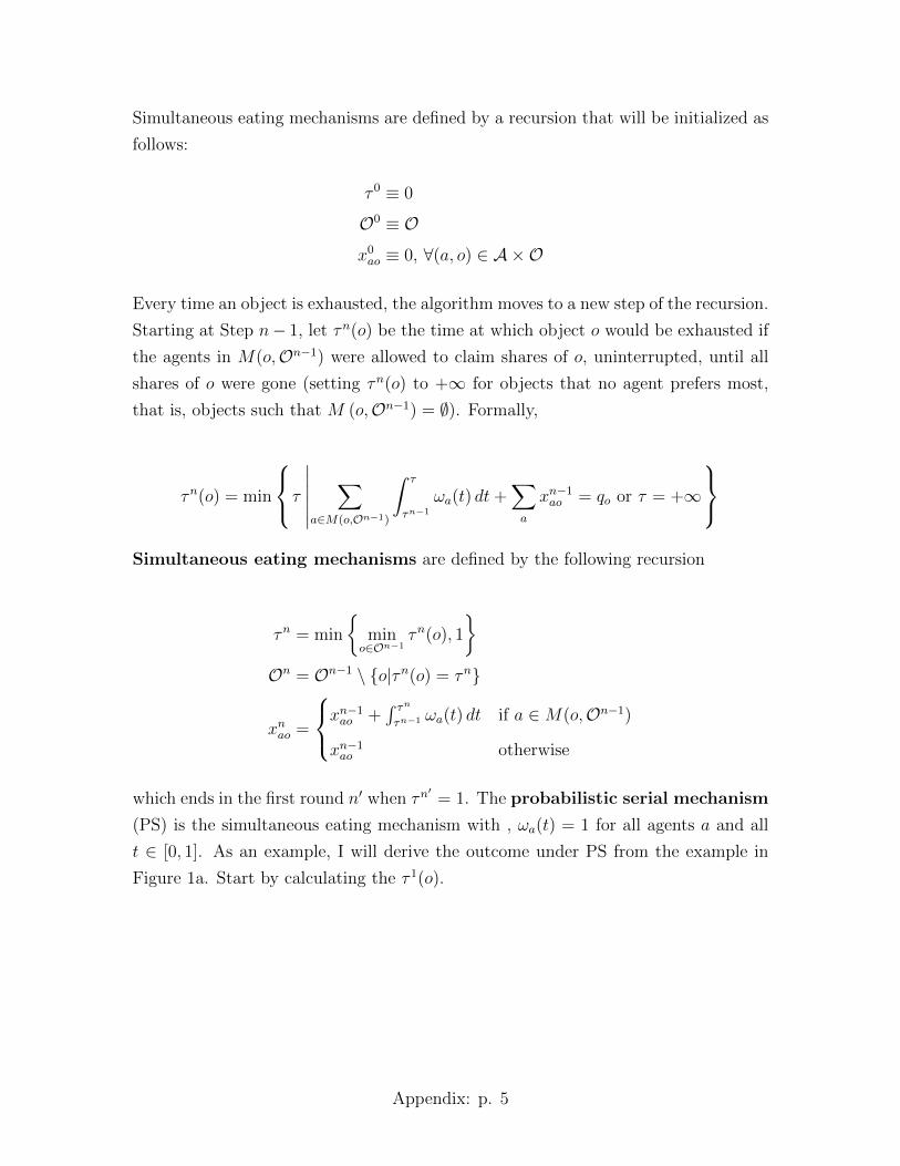
Simultaneous eating mechanisms are defined by a recursion that will be initialized as

follows:

τ 0 ≡ 0

O0 ≡ O

x0ao ≡ 0, ∀(a, o) ∈ A×O

Every time an object is exhausted, the algorithm moves to a new step of the recursion.

Starting at Step n− 1, let τn(o) be the time at which object o would be exhausted if

the agents in M(o,On−1) were allowed to claim shares of o, uninterrupted, until all

shares of o were gone (setting τn(o) to +∞ for objects that no agent prefers most,

that is, objects such that M (o,On−1) = ∅). Formally,

τn(o) = min

τ∣∣∣∣∣∣

∑a∈M(o,On−1)

ˆ τ

τn−1

ωa(t) dt+∑a

xn−1ao = qo or τ = +∞

Simultaneous eating mechanisms are defined by the following recursion

τn = min

min

o∈On−1τn(o), 1

On = On−1 \ o|τn(o) = τn

xnao =

xn−1ao +

´ τnτn−1 ωa(t) dt if a ∈M(o,On−1)

xn−1ao otherwise

which ends in the first round n′ when τn′= 1. The probabilistic serial mechanism

(PS) is the simultaneous eating mechanism with , ωa(t) = 1 for all agents a and all

t ∈ [0, 1]. As an example, I will derive the outcome under PS from the example in

Figure 1a. Start by calculating the τ 1(o).

Appendix: p. 5

τ 1(a) =1

2

τ 1(b) = 1

τ 1(c) = +∞

τ 1(d) = +∞

Hence, τ 1 = 1/2, O1 = b, c, d, and

x1 =

a b c d

1 : 1/2 0 0 0

2 : 1/2 0 0 0

3 : 0 1/2 0 0

Now, t1(a) =∞, and

τ 1(b) = 3/4

τ 1(c) = 3/2

τ 1(d) = +∞

Hence, τ 2 = 3/4, O2 = c, d, and

x2 =

a b c d

1 : 1/2 0 1/4 0

2 : 1/2 1/4 0 0

3 : 0 3/4 0 0

Finally, τ 2(a) = τ 2(b) =∞, and

τ 1(c) = 9/8

τ 1(d) = 7/4

Hence, τ 2 = 1, and the final probabilistic serial assignment is

Appendix: p. 6

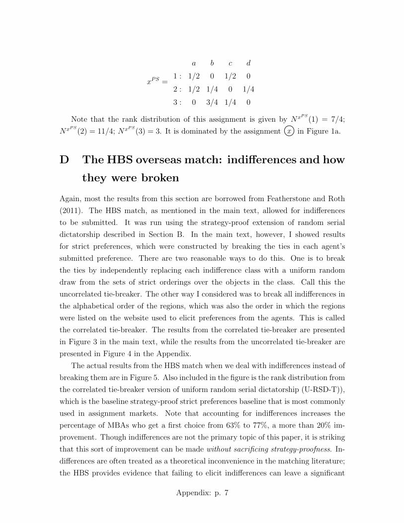
xPS =

a b c d

1 : 1/2 0 1/2 0

2 : 1/2 1/4 0 1/4

3 : 0 3/4 1/4 0

Note that the rank distribution of this assignment is given by NxPS(1) = 7/4;

NxPS(2) = 11/4; NxPS(3) = 3. It is dominated by the assignment x© in Figure 1a.

D The HBS overseas match: indifferences and how

they were broken

Again, most the results from this section are borrowed from Featherstone and Roth

(2011). The HBS match, as mentioned in the main text, allowed for indifferences

to be submitted. It was run using the strategy-proof extension of random serial

dictatorship described in Section B. In the main text, however, I showed results

for strict preferences, which were constructed by breaking the ties in each agent’s

submitted preference. There are two reasonable ways to do this. One is to break

the ties by independently replacing each indifference class with a uniform random

draw from the sets of strict orderings over the objects in the class. Call this the

uncorrelated tie-breaker. The other way I considered was to break all indifferences in

the alphabetical order of the regions, which was also the order in which the regions

were listed on the website used to elicit preferences from the agents. This is called

the correlated tie-breaker. The results from the correlated tie-breaker are presented

in Figure 3 in the main text, while the results from the uncorrelated tie-breaker are

presented in Figure 4 in the Appendix.

The actual results from the HBS match when we deal with indifferences instead of

breaking them are in Figure 5. Also included in the figure is the rank distribution from

the correlated tie-breaker version of uniform random serial dictatorship (U-RSD-T)),

which is the baseline strategy-proof strict preferences baseline that is most commonly

used in assignment markets. Note that accounting for indifferences increases the

percentage of MBAs who get a first choice from 63% to 77%, a more than 20% im-

provement. Though indifferences are not the primary topic of this paper, it is striking

that this sort of improvement can be made without sacrificing strategy-proofness. In-

differences are often treated as a theoretical inconvenience in the matching literature;

the HBS provides evidence that failing to elicit indifferences can leave a significant

Appendix: p. 7

60%

65%

70%

75%

80%

85%

90%

95%

100%

1 2 3 4 5 6 7 8 9 10 11

Ran

ked

kth

or

bet

ter

k

U-RSD

PS

RVM

Figure 4: Results from the uncorrelated tie-breaker(U-RSD is Uniform Random Serial Dictatorship, PS is Probabilistic Serial, and RVM is Rank-Value

Mechanism. Note that U-RSD and PS overlap.)

amount of welfare on the table.

E Proofs

E.1 Rank efficiency

E.1.1 Characterization of rank-value mechanisms

Here, I generalize Theorem 1 to the α-rank efficiency concept defined in Section 9.

Generalization of Theorem 1. x is an α-rank efficient assignment if and only if

there exists a valuation v such that x is supported by the (α, v)-rank-value mechanism.

Proof. Start by proving the “if” part. The objective of the defining linear program

can be rewritten as|O|−1∑k=1

Nxα(k) (vk − vk+1) + |A| · v|O|. By way of contradiction, let x

Appendix: p. 8

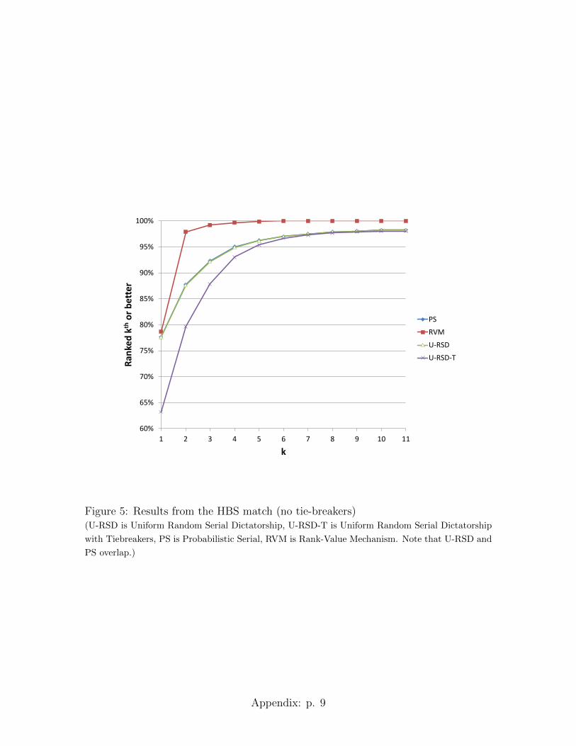
60%

65%

70%

75%

80%

85%

90%

95%

100%

1 2 3 4 5 6 7 8 9 10 11

Ran

ked

kth

or

bet

ter

k

PS

RVM

U-RSD

U-RSD-T

Figure 5: Results from the HBS match (no tie-breakers)(U-RSD is Uniform Random Serial Dictatorship, U-RSD-T is Uniform Random Serial Dictatorship

with Tiebreakers, PS is Probabilistic Serial, RVM is Rank-Value Mechanism. Note that U-RSD and

PS overlap.)

Appendix: p. 9

be a random assignment that α-rank-dominates the allocation yielded by the (α, v)-

rank-value mechanism, x∗. Then, the following is true:

|O|−1∑k=1

N xα(k) · (vk − vk+1) + |A| · v|O| >

|O|−1∑k=1

Nx∗

α (k) · (vk − vk+1) + |A| · v|O|

because the α-rank dominance of x over x∗ means that the left-hand side is weakly

greater than the right-hand side, term by term, and strictly so for at least one term.

But this is a contradiction of the optimality of the (α, v)-rank-value mechanism’s

defining linear program.

Now, I prove the “only if” part. Let Aα ⊂ R|O|−1 denote the set of α-rank

distributions that can be generated some random assignment, where the first index

of the vector corresponds to Nxα(1), the second to Nx

α(2), and so on. By the definition

of an α-rank distribution, Aα is convex. Now, let b ∈ Aα be the α-rank distribution

generated by x, the α-rank efficient assignment from the hypothesis of the theorem.

The set of α-rank distributions that would α-rank dominate b if they were generated

by feasible random allocations is U(b) ≡a∣∣a ∈ R|O|−1; ai ≥ bi, ∀i; ∃i′, ai > bi

. U(b)

is also convex. Any member of both Aα and U(b) would α-rank dominate x, so it

must be that Aα ∩ U(b) = ∅. The separating hyperplane theorem then tells us that

there is some p 6= 0 and some c such that p · u ≥ c,∀u ∈ U(b) and p · a ≤ c, ∀a ∈ Aα.

By construction, p · b = c. Without loss of generality, assume c ≥ 0. Now, let ei

denote the unit vector that points along the ith axis of R|O|−1. For any δ>0 , it must

be that b+ δei ∈ U(b). This means that p · (b+ δei) = c+ δpi ≥ c, which means that

pi ≥ 0. Consider the valuation v where vi = 1 +|O|−1∑j=i

pj, ∀i ∈ 1, . . . , |O| − 1, and

v|O| = 1. By construction, the (α, v)-rank-value mechanism supports x. But because

I have yet to prove that pi > 0,∀i, I am not sure that v is a valid valuation, that is

vk > vk+1,∀k.

To show this will require the stronger Polyhedral Separating Hyperplane Theorem

of McLennan (2002). Adopting the notation of that paper’s Theorem 2, let P =

Aα−R|O|−1 (which is a polyhedron by Theorem 1.2 of Ziegler (1995)) and b = p ∈ P .

The α-rank efficiency of x tells us that x is not in the relative interior70 of P , so the

Theorem lets us conclude that there is a hyperplane H such that P is contained in

one of its half-spaces, P ⊂ H−, and F ≡ P ∩H is the smallest face of P that contains

70The relative interior of a set S is its interior in the relative topology of its affine hull. The affinehull of S is the set of all affine combinations of elements of S. An affine combination of a set ofelements s1, . . . , sk of S is a sum

∑i αi · si, where αi ∈ R,∀i and

∑ki=1 αi = 1.

Appendix: p. 10

b. Pick p and c such that H =u ∈ R|O|−1

∣∣p · u = c

. First, note that for δ > 0,

b − δei ∈ P , by definition. Now, say that pi = 0. Then, b − δei ∈ H as well, which

means that b− δei ∈ F . Lemma 2 of McLennan (2002) with S = b tells us that the

relative interior of S, that is b,71 is contained in the relative interior of the smallest

face that contains S, that is F . Hence, for some δ > 0 small enough, b + δei ∈ F .

But since F ⊂ P , this contradicts our original assumption of the α-rank-efficiency of

x. Hence, pi > 0, ∀i.

E.1.2 Rank-improving cycles and improvement cycles

Without changing the number of copies of the objects (including ∅), consider adding∑o qo−|A| dummy agents to the market that are indifferent between all the objects.

Call this the augmented market. Note that the dummy agents are different from

the fictional agent introduced in the definition of claim-trade cycles.72 The extension

of x to the augmented market is an assignment x in which all real agents’ allocations

stay the same and the remaining objects are feasibly assigned to the dummy agents.

Lemma 1. Let x be the extension of x to the augmented market. Then, x is non-

wasteful if and only if there does not exist an improvement cycle in x that includes a

dummy agent.

Proof. (“only if”) If there is an improvement cycle that includes a dummy agent, then

there is also a two agent improvement cycle where one of the agents is the dummy.

Since the dummy is indifferent between all the objects and is holding something that

was not assigned in x, this cycle is equivalent to the real agent claiming something

that was not assigned, contradicting the assumption that x was non-wasteful. (“if”)

If x is wasteful, then x must have a two person improvement cycle between the real

agent who wants to claim an object unassigned under x and the dummy agent who

was assigned that object in x.

Proposition 7 (Bogomolnaia and Moulin 2001). An assignment x is ordinally effi-

cient if and only if x is non-wasteful and admits no improvement cycles.

Proof. This is proven with |A| =∑

o qo for preferences with indifferences in Katta and

Sethuraman (2006), and without indifferences by Bogomolnaia and Moulin (2001).

Ordinal efficiency in a market with |A| >∑

o qo is equivalent to ordinal efficiency in

71The affine hull of b is b.72The fictional agent is, in some sense, a “super” dummy that owns the shares held by all of the

smaller dummies.

Appendix: p. 11

the augmented market, so ordinal efficiency is equivalent to no cycles in the augmented

market. A cycle in the augmented market either contains a dummy or doesn’t, so

by Lemma 1, a cycle in the augmented market is equivalent to either a cycle or

wastefulness in the regular market.

Before addressing α-rank efficiency, I re-introduce the generalization of a v-rank-

improving cycle that was relegated to Footnote 62 in the main text.

Definition 16. A trade cycle τ on assignment x is an (α, v)-rank-improving cycle

if

|τ |∑k=1

αak ·[vrak (ok−1) − vrak (ok)

]> 0 (with o0 ≡ o|τ |).

Lemma 2. Let x be the extension of x to the augmented market. Then, x admits no

(α, v)-rank improving cycles if and only if x admits no (α, v)-rank improving cycles.

Remark 8. Note that while there can claim-trade cycles in x, there can’t in x, since

by construction, all object shares are claimed.

Proof. (“only if”) By way of contradiction, assume that τ is an (α, v)-rank improving

cycle in x. If τ has exactly one dummy, then it is already an (α, v)-rank improving

claim-trade cycle in x, a contradiction. If τ has multiple dummies, then it can be par-

titioned into several claim-trade cycles in x by taking the parts between any dummy

and the next dummy in τ . Because τ is overall (α, v)-rank improving, at least one

of the elements of the partition must be an (α, v)-rank improving claim-trade cycle

in x, a contradiction. Obviously, if τ has no dummies, then it is also an (α, v)-rank

improving trade cycle in x, a contradiction. (“if”) By way of contradiction, assume

that τ is an (α, v)-rank improving claim-trade cycle in x. Then an (α, v)-rank im-

proving trade cycle can be constructed in x by letting a1 be a dummy that is holding

o1, a contradiction. Now, assume that τ is an (α, v)-rank improving trade cycle in x.

It must also be an (α, v)-rank improving trade cycle in x, a contradiction.

Generalization of Theorem 2. x is α-rank efficient if and only if there exists a

valuation v such that x admits no (α, v)-rank-improving cycles.

Proof. (“only if”) By way of contradiction, assume that for any valuation v, there

exists an (α, v)-rank improving cycle. This would yield an improvement in the ob-

jective of the (α, v)-rank-value mechanism, which means that x cannot be generated

by any (α, v)-rank-value mechanism, which, by the Generalization of Theorem 1 in

Section E.1.1 of the Appendix, means that x is not α-rank efficient.

Appendix: p. 12

(“if”) Consider the extension of x to the augmented market, x. Now, by way of

contradiction, let x α-rank dominate x in that market. Let ξ ≡ x − x. Necessarily,∑o ξao = 0 and

∑a ξao = 0. Construct a cycle by the following procedure. First,

find some (a1, o1) such that ξa1o1 < 0. Then, find some a2 such that ξa2o1 > 0. Next,

find some o2 such that ξa2o2 < 0. In words, this process starts by picking a negative

element in ξ, then goes down the column to a positive element, then across the row

to a negative element, and so on. Continue building a sequence of agents and objects

in this way, until an agent is visited twice, i.e., a cycle is found. This process is

well-defined because any row or column with a non-zero element must have another

non-zero element of the opposite sign, since all rows and columns sum to zero. The

process will eventually terminate because the market is finite. By construction, the

process finds sequence of agents and objects that is a trade cycle. Denote it by τ .

Now, let Ξ = min(a,o)∈τ

|ξao| and define:

ξ1ao =

Ξ ∃k s.t. (a, o) = (ak, ok)

−Ξ ∃k s.t. (a, o) = (ak+1, ok)

0 otherwise

Then ξ− ξ1 has at least one fewer non-zero entries than ξ. Hence, this process can be

repeated to decompose ξ into a sum of trade cycles, that is ξ =∑

i ξi where each ξi

represents a trade cycle in the augmented market. Then, x = x +∑

i ξi. Now, since

x α-rank dominates, the objective of the (α, v)-rank-value mechanism is bigger at x,

regardless of the valuation. By the linearity of the objective of the (α, v)-rank-value

mechanism, it cannot be that the value of the objective evaluated at ξi is weakly

negative for all i. In other words, regardless of the valuation, at least one of the ξis

must be (α, v)-rank improving, which by Lemma 2 means that there is an (α, v)-rank

improving cycle in x, which by Lemma 2 is equivalent to an (α, v)-rank improving

cycle in x, a contradiction.

Proposition 4. If all elements of the initial assignment matrix are rational numbers,

then the sequential improvement process will terminate in a finite number of steps with

a rank efficient assignment that is in the arg max of the v-rank-value mechanism.

Proof. Implementing an (α, v)-rank-improving cycle transforms deterministic assign-

ments into deterministic assignments. It also necessarily increases the objective of

the (α, v)-rank-value mechanism, so the algorithm cannot cycle. Since the set of de-

Appendix: p. 13

terministic assignments is finite, the algorithm must terminate. Note that the same

logic works if all entries in the initial matrix are rational: simply multiply the starting

matrix by the least common denominator.

Lemma 3. Let x be a deterministic assignment. Then x is ex post efficient if and

only if it is non-wasteful and admits no improvement cycles.

Proof. The “only if” follows from the fact that implementing any improvement cycle

in the augmented market immediately yields an ex post dominator. For the “if” part,

consider the extension of x to the augmented market, x and assume it has an ex post

dominator, x. Using the decomposition strategy of the proof to the Generalization of

Theorem 2, one can move from x to x through a series of trade cycles. But, because

both x and x are deterministic assignments, for all the trade cycles, Ξ will equal 1.

Hence, each agent can only be involved in, at most, one of the trade cycles, and hence,

all of the trade cycles must be improvement cycles. By Lemma 1, these cycles map

back to either an improvement cycle, or wastefulness in x, a contradiction.

Proposition 8. Let x be a deterministic assignment. Then,

(i) x is ordinally efficient if and only if it is ex post efficient.

(ii) x is rank efficient implies it is ex post efficient; however the converse need not

hold.

Proof. Part (i) follows directly from Proposition 7 and Lemma 3. Now, I prove (ii).

Proposition 3 establishes that rank efficiency implies ex post efficiency. To see that

the converse need not hold, consider x© and y from Figure 1a. Both are ex post

efficient deterministic assignments, but only one is rank efficient.

E.1.3 Ex ante efficiency interpretation

The proof in the main text only addresses uniform weights. To justify an (α, v)-

rank-value mechanism, I need αa ·´va′k · F (v) = αa′ ·

´vak · F (v). In other words,

the unconditional expectations of va for all agents should be proportional, and the

constants of proportionality should be the appropriate weights from the α vector.

E.2 Truth-telling in low information environments

I allow for indifferences and a general weighting of the agents in all theorems I will

be deriving, so when I generalize relative to a statement in the main text, I will

Appendix: p. 14

note that I have done so . The general scheme of the proofs in this section borrow

heavily from Roth and Rothblum (1999), but the proofs themselves are new, as they

must be adapted to the rank-value mechanism, which is quite different from the more

algorithmically defined deferred acceptance algorithm. Let RVMα,va (%; q; τ) denote

a’s allocation under the (α, v)-rank-value mechanism when the submitted preferences

are %, the capacities are q, and the tie-breaker ordering is τ . Let the objective

function of the (α, v)-rank-value mechanism evaluated at assignment x and submitted

preferences % be denoted by

V α,v(%;x) ≡∑a′′

∑o′′

αa′′ · vra′′ (o′′) · xa′′o′′

Lemma 4. Let o′ a o. Then,

[RVMα,va (%; q; τ) = o]⇒

[RVMα,v

a

(%o↔o′a ,%−a; q; τ

)= o]

Proof. Swapping o and o′ changes the objective in the following way:

V α,v(%o↔o′a ,%−a;x

)= V α,v(%;x) + αa ·

(vra(o′) − vra(o)

)· (xao − xao′) (1)

Now, let y = RVMα,v (%; q; τ), which tells us that yao = 1 and yao′ = 0, which means

V α,v(%; y)− V α,v(%o↔o′a ,%−a; y

)= −αa ·

(vra(o′) − vra(o)

)< 0

Now consider another assignment z 6= y that is a member of the arg max of the linear

program when when o and o′ are switched, that is

V α,v(%o↔o′a ,%−a; z

)≥ V α,v

(%o↔o′a ,%−a; y

)(2)

First, I show that zao = 1. Assume otherwise. Then, by Equation 1, I derive

V α,v (%; z)− V α,v(%o↔o′a ,%−a; z

)≥ 0 > V α,v (%; y)− V α,v

(%o↔o′a ,%−a; y

)If I add this inequality to Inequality 2, I find that y was not an optimum to start

with, a contradiction. Hence, a must receive o when he switches. Now, if zao = 1,

then following the same logic, I derive

V α,v (%; z)− V α,v(%o↔o′a ,%−a; z

)= V α,v (%; y)− V α,v

(%o↔o′a ,%−a; y

)

Appendix: p. 15

and combine it with Inequality 2 to find that either y was not an optimum to start

with (a contradiction), or that z is a member of the arg max under both normal and

switched preferences. But then, the only way that z could be chosen under the switch

is if τ(z) < τ(y), which would contradict y being chosen under the truth.

Corollary (to Lemma 4). Let o′ a o. Then,[RVMα,v

a

(%o↔o′a ,%−a; τ

)= o′

]⇒ [RVMα,v

a (%; τ) = o′]

Proposition 9. Under a rank-value mechanism, if agent a’s beliefs are o, o′-symmetric,

and o′ a o, then for a, the allocation resulting from any submitted preference that

declares o a o′ is weakly stochastically dominated by the allocation resulting from a

submitted preference that does not. If the beliefs are symmetric, then this holds for

all o, o′ ∈ O \ ∅.

Proof. First, note that since the linear program does not depend on labels,

[RVMα,va (%; q; τ) = v]⇔

[RVMα,v

a

(%o↔o′ ; qo↔o

′; τ o↔o

′)

= v]

[RVMα,va (%; q; τ) = o]⇔

[RVMα,v

a

(%o↔o′ ; qo↔o

′; τ o↔o

′)

= o′]

where o, o′ ∈ O and v ∈ O \ o, o′. Then, it must also be that

[RVMα,v

a

(o↔o′a ,%−a; q; τ

)= v]⇔[RVMα,v

a

(%a,%

o↔o′−a ; qo↔o

′; τ o↔o

′)

= v]

[RVMα,v

a

(%o↔o′a ,%−a; q; τ

)= o]⇔[RVMα,v

a

(%a,o↔o

′

−a ; qo↔o′; τ o↔o

′)

= o′]

Now, using Lemma 4 and its corollary, one can think about the gains and losses an

agent a who prefers o′ to o gets from switching those two objects. The possible cases

are shown in Table 2. Using these cases, one can then think about what our agent

gets when everyone else’s preferences switch o and o′, which is equally likely due to

the assumption of o, o′-symmetric beliefs. This analysis is shown in Table 3. In

each of the cases, considering that everyone else switching o and o′ is equally likely,

truth-telling yields an allocation for a that weakly stochastically dominates what she

would have gotten by switching o and o′.

The condition in Proposition 9 is important enough to warrant a name.

Appendix: p. 16

Lie: RVMα,va

(%o↔o′a ,%−a; q; τ

)= u /∈o, o′ = o′ = o

= v /∈ o, o′ Case A Impossible Case B

Truth: RVMa (%a,%−a; q; τ) = o′ Case C Case D Case E

= o Impossible Impossible Case F

Table 2: Cases

a tells the truth a switches o and o′

(%a,%−a; q; τ)(%a,%o↔o

′−a ; qo↔o

′; τo↔o

′) (

%o↔o′

a ,%−a; q; τ) (

%o↔o′

a ,%o↔o′

−a ; qo↔o′; τo↔o

′)

Case A v u u v

Case B v o′ o v

Case C o′ u u o

Case D o′ o o′ o

Case E o′ o′ o o

Case F o o′ o o′

Table 3: Assignments under the different cases

Definition 17. A reported preference %′a is called weakly o, o′o, o′o, o′-order-preserving

with respect to %a%a%a if [o′ a o]⇒ [o′ %′a o]. If this is true for all o, o′ ∈ O\∅, then

just call the reported preference weakly order-preserving with respect to %a%a%a.

Notice that if I am dealing with a world where only strict preferences are allowed,

then this property basically says that objects besides ∅ are listed in their true order,

which is where I get Theorem 4. If I allow for indifferences, then I am not insisting on

truthful ordering, but instead are insisting that a true strict ordering of two objects is

never reported reversed. Before moving on, I review a notation that was only briefly

introduced in the main text. Let the true preference be %a and the preference that

adds an indifference class I of objects right above ∅ be %+Ia . For some object o, let

%+oa denote %+o

a .

Lemma 5. If the ranking scheme is upward-looking and unmatched-distinct then,

submitting a preference where the bottom declared-acceptable indifference class con-

sists entirely of truly unacceptable objects is weakly stochastically dominated by the

submitting the same preference with the bottom declared-acceptable indifference class

dropped.

Appendix: p. 17

Proof. By way of contradiction, assume that I is a set of unacceptable objects,

and that submitting %+Ia makes a better off, that is RVMa

(%+Ia ,%−a; q; τ

)≡ z,

RVMa (%; q; τ) ≡ y, and ya ≺a za. Then, by optimality, I know that V (%; y) ≥V (%; z) and V

(%+Ia ,%−a; z

)≥ V

(%+Ia ,%−a; y

). Now, ya is necessarily not in the

lowest indifference class of %+Ia , but it could either be in a higher indifference class,

or it could be ∅.

Case 1. (ya is ranked above %+Ia ) za must also be ranked above the bottom accept-

able indifference class of %+Ia , so (since I have assumed that the rankings

are upward-looking) V(%+Ia ,%−a; y

)= V (%; y) and V

(%+Ia ,%−a; z

)=

V (%; z). Combined with the optimality inequalities, these equalities im-

ply that y and z are both in the arg max under both preferences. This

cannot be, since the tiebreaker τ would choose one or the other.

Case 2. (ya = ∅) za is necessarily not in the lowest acceptable indifference class

of %+Ia , so V

(%+Ia ,%−a; z

)= V (%; z). Now since the ranking scheme

is unmatched-distinct, V(%+Ia ,%−a; y

)= V (%; y). Stringing inequalities

together, I find that y and z are both in the arg max under both preferences.

This cannot be, since the tiebreaker τ would choose one or the other.

Lemma 6. If the ranking scheme is upward-looking and unmatched-neutral, then if

o is a truly acceptable object that is declared unacceptable in %a, then

RVMα,va (%; q; τ) -a RVM

α,va

(%+oa ,%−a; q; τ

)Proof. Define y ≡ RVMα,v (%; q; τ) and z ≡ RVMα,v (%+o

a ,%−a; q; τ). Since y is an

arg max under %, I have V α,v (%; y) ≥ V α,v(%; z), and since z is an arg max under

(%+oa ,%−a), I have V α,v (%+o

a ,%−a; z) ≥ V α,v(%+oa ,%−a; y).

Now, by way of contradiction, assume that ya a za. There are three cases.

Case 1. (za = ∅) The ranking scheme is unmatched-neutral, so V α,v(%; z) > V α,v(%+oa

,%−a; z). Since ya is above the part of the rank-order that has changed, I

know V α,v(%+oa ,%−a; y) = V α,v(%; y) by the upward-looking assumption.

Combined with the optimality inequalities, I quickly arrive at a contradic-

tion.

Case 2. (za = o) Denote by z|(a,∅) the assignment I get by starting with z and only

moving a from o to ∅. This is feasible, so since y is an arg max under %, I

Appendix: p. 18

know that V α,v (%; y) ≥ V α,v(%; z|(a,∅)) By unmatched-neutrality, V α,v(%

; z|(a,∅)) = V α,v(%+oa ,%−a; z) Again, since ya is above any changes to the

rank orders, V α,v(%; y) = V α,v(%+oa ,%−a; y). Combined with the fact that

z is an arg max under (%+oa ,%−a), I can deduce that all of these objective

values must be equal. But if this were true, there would no way that the

same tiebreaker τ could have chosen two different assignments.

Case 3. (za a o) Both za and ya are above any changes in the rank orders. Hence,

by the upward-looking assumption, z and y must be in the arg max for

both submitted preferences, and since I break ties by choosing the lowest

τ , it is a contradiction that I choose y under the true preferences and z

under the truncations.

Proposition 13. Assume that agent a’s beliefs are symmetric. If the ranking scheme

is upward-looking and unmatched-neutral, then truly acceptable objects must be de-

clared acceptable. If the ranking scheme is upward-looking and unmatched-distinct,

then any unacceptable objects that a declares acceptable must be in the bottom indif-

ference class and declared indifferent to some acceptable objects.

Proof. The previous lemma establishes the first part of the theorem. For the second

part, note that symmetry requires that the objects are submitted in a weakly order

preserving way. Hence, there can exist only one indifference class that contains both

unacceptable and acceptable objects. Below that indifference class, all classes must

be filled with unacceptable objects. By Lemma 5, I can drop them.

This combined with Proposition 9 gives us the generalization of Theorem 5 to

preferences with indifferences.

Generalization of Theorem 5. If an agent’s beliefs are symmetric and the rank

scheme is upward-looking and...

• ...unmatched-distinct, then his expected allocation from any other strategy is

weakly stochastically dominated by his expected allocation from submitting some

weakly order preserving preference in which any truly unacceptable objects that

are declared acceptable are declared indifferent to some truly acceptable object

and are declared in the lowest acceptable indifference class.

Appendix: p. 19

• ...unmatched-neutral, then his expected allocation from any other strategy is

weakly stochastically dominated by his expected allocation from submitting some

weakly order preserving preference in which all truly acceptable objects are de-

clared acceptable.

E.3 Supportable rank efficiency

Theorem 6. Supportable rank efficiency implies ordinal efficiency. The converse

need not hold.

Proof. To show the positive statement, note that supportable rank efficiency im-

plies, for some α, α-rank efficiency, which in turn, for any α, implies ordinal effi-

ciency. To see that the converse need not hold, start by defining ∆(α,v)τ V =

|τ |∑m=1

αam ·(vram (om−1)−vram (om)

)for a trade cycle τ (where o0 ≡ om). By the Generalization of

Theorem 2 in Section E.1.2, an assignment is only supportably rank efficient there

exists some (α, v) such that ∆(α,v)τ V ≤ 0 for all trade cycles τ . Now, consider a 6

agent example, where there is one seat at a through d and 2 seats at e.

1 : a d e

2 : a c e

3 : a b e

4 : b c e

5 : c d e

6 : b e

Probabilistic serial yields the random allocation

a b c d e

1 : 1/3 0 0 17/27 1/27

2 : 1/3 0 7/27 0 11/27

3 : 1/3 1/9 0 0 15/27

4 : 0 4/9 4/27 0 11/27

5 : 0 0 16/27 10/27 1/27

6 : 0 4/9 0 0 15/27

which I know to be ordinally efficient. Relative to the trade cycles

Appendix: p. 20

τ1 = ((1, a) , (2, e))

τ2 = ((1, e) , (2, a))

τ3 = ((1, a) , (3, b) , (4, c) , (5, d))

τ4 = ((1, a) , (2, e) , (3, b) , (4, c) , (5, d))

I can calculate how ∆(α,v)τ V will change:

∆(α,v)τ1 V = (α2 − α1) · (v1 − v3)

∆(α,v)τ2 V = (α1 − α2) · (v1 − v3)

∆(α,v)τ3 V = (α3 + α4 + α5 − α1) · (v1 − v2)

∆(α,v)τ4 V = −α1 · (v1 − v2) + α2 · (v1 − v3)− α3 · (v2 − v3) + (α4 + α5) · (v1 − v2)

Now, I show how there is no (α, v) such that one of these trade cycles isn’t (α, v)-

rank improving, that is ∆(α,v)τ V ≤ 0. Since v1 > v3, I need α1 = α2 to prevent

either τ1 and τ2 from being (α, v)-rank-improving. To prevent τ3 from being α-rank-

improving, I need α1 ≥ α3 +α4 +α5. Finally, since α1 = α2, I can simplify ∆(α,v)τ4 V to

(α1−α3)·(v2−v3)+(α4+α5)·(v1−v2). The second term is definitely positive, so it must

be that α1 < α3. But combining the last two inequalities gives us α3 > α3 + α4 + α5,

which cannot be. Hence, there is no (α, v) such that ∆(α,v)τ V ≤ 0 for all four of the

trade cycles I have listed. Thus the ordinally efficient assignment I started with is

not supportably rank efficient.

E.4 Competitive equilibrium mechanisms

To establish Theorem 7, I will be using the concept of a discount equilibrium.

Definition 18. Prices and an assignment, (x∗, p), form a discount equilibrium with

respect to weights ααα and valuation vvv (or just (α,v)-discount equilibrium) if, for

all a,

x∗a ∈ arg maxxa≥0

∑o

(vra(o) − po

αa

)· xao

s.t.∑o

xao ≤ 1

and

Appendix: p. 21

x∗ao ∈ arg maxxao≥0

∑a

∑o

po · xao

s.t.∑a

xao ≤ qo ,∀o

(α, v)-discount equilibria decentralize the linear program that defined the (α, v)-

rank-value mechanism. Formally,

Proposition 14. x is α-rank efficient if and only if there exist prices p, and a valu-

ation v, such that (x∗, p) form an (α, v)-discount equilibrium

Proof. First, I prove the “only if” part. Since x is α-rank efficient, there must be a

valuation such that it is in the arg max of the (α, v)-rank-value mechanism, by the

Generalization of Theorem 1 in Section E.1.1.

The LP dual of the (α, v)-rank efficient mechanism is

minua≥0,po≥0

∑o∈O

qo · po +∑a∈A

αa · ua

s.t. ua ≥ vra(o) − poαa

∀o ∈ O, a ∈ A

I will support the discount equilibrium with the prices from the dual of the rank

efficient mechanism. Now, the LP dual of the agent a’s problem in the (α, v)-discount

equilibrium with these prices is

minua

ua

s.t. ua ≥ vra(o) − poαa∀o ∈ O

By nested optimization, I see that the ua from the rank efficient mechanism’s

dual also solves the discount equilibrium duals. Now, let xao be the assignment I

are considering from the arg max of the rank efficient mechanism. The LP duality

theorem tells us that

∑o∈O

qo · po +∑a∈A

αa · ua =∑a∈A

∑o∈O

αa · vra(o) · xao

From the constraint in the dual of the rank efficient mechanism, I can then derive

that, for any ξ such that∑

o ξao ≤ 1,∀a ∈ A, I have

∑o∈O

qo · po +∑a∈A

αa ·∑o∈O

(vra(o) −

poαa

)· ξao ≤

∑a∈A

∑o∈O

αa · vra(o) · xao (3)

If I plug in x for ξ, then this reduces to∑

o∈O po ·(qo −

∑a∈A xao

)≤ 0. Since

all elements of that sum are weakly positive, I conclude that po ·(qo −

∑a∈A xao

)=

Appendix: p. 22

0,∀o ∈ O. This, coupled with a constraint from the rank efficient mechanism, is the

second condition of the discount equilibrium. Note that I have also shown that

∑o∈O

qo · po +∑a∈A

αa ·∑o∈O

(vra(o) −

poαa

)· xao =

∑a∈A

∑o∈O

αa · vra(o) · xao

Finally, I show that the xao from the arg max of the rank efficient mechanism must

also be part of the arg max for the agents’ problems in the discount equilibrium.

By way of contradiction, say that they aren’t, and let ξa be the bundle chosen by

agent a under prices p. Then, for all agents,∑

o ξao ≤ 1 and∑

o

(vra(o) − po

αa

)· ξao ≥∑

o

(vra(o) − po

αa

)· xao, with the second inequality strict for some agent a′. Thus,

∑o∈O

qo ·po+∑a∈A

αa ·∑o

(vra(o) −

poαa

)·ξao >

∑o∈O

qo ·po+∑a∈A

αa ·∑o

(vra(o) −

poαa

)·xao

But I have shown∑o∈O

qo · po +∑a∈A

αa ·∑o

(vra(o) −

poαa

)· xao =

∑a∈A

∑o∈O

αa · vra(o) · xao,

which means that I have derived∑o∈O

qo · po +∑a∈A

αa ·∑o

(vra(o) −

poαa

)· ξao >

∑a∈A

∑o∈O

αa · vra(o) · xao

which stands in direct contradiction to something I have already proven, Inequality 3.

Therefore, the assignment from the rank efficient mechanism solves the agents’ prob-

lems in the discount equilibrium. Thus I have shown that any member of the arg

max of the rank efficient equilibrium can be supported as a discount equilibrium.

Now, I prove the “if” part. Consider the optimization

maxx

∑o

∑a

αa · vra(o) · xao +∑o

po ·(qo −

∑a

xao

)s.t.

∑o

xao ≤ 1∑a

xao ≤ qo

By the positivity of the prices and the object quota constraints, the value of this

optimization is greater than or equal to the value of

Appendix: p. 23

maxx

∑o

∑a

αa · vra(o) · xao

s.t.∑o

xao ≤ 1∑a

xao ≤ qo

Now, if I start with the assignment x from some discount equilibrium, it will also

solve the first optimization. To see this, relax the optimization by removing the object

capacity constraints. The relaxation can then be separated into an optimization for

each agent that is equivalent to the agent’s problem from the discount equilibrium,

so x solves the relaxation. But, since x is part of a discount equilibrium, it also meets

the object capacity constraints, and is thus an optimizer of the full problem as well.

By the seller’s problem in the discount equilibrium (see Remark 7), the value of this

assignment in the first optimization is attained in the second as well. Hence, x must

solve the second optimization, since it attains the upper bound at x. Hence, x is

in the arg max of the (α, v)-rank-value mechanism’s defining program, which means

that x is α-rank efficient.

This is a strange decentralization, as it distorts prices in a way that one might

expect it to not yield any sort of efficiency. At the end of this section, I will discuss

the intuition for why the discount equilibrium decentralization remains efficient.

Proposition 15. There exist weights α such that (x, p) is an (α, v)-discount equilib-

rium if and only if there exist budgets B such that (x, p) is a (B, v)-budget equilibrium.

Proof. I start by showing that if I start with an (α, v)-discount equilibrium (x∗, p),

then it is also a (B, v)-budget equilibrium for Ba =∑o

po · x∗ao. By way of con-

tradiction, assume that (x∗, p) is not a (B, v)-budget equilibrium assignment for

B. By construction, it is feasible, so it must be that there is some other feasi-

ble x such that∑o

vra(o) · xao >∑o

vra(o) · x∗ao. Since it is feasible, I also know that∑o

po · xao ≤∑o

po · x∗ao. Combining the last two inequalities (multiplying the second

by 1/αa), I find∑o

(vra(o) − po

αa

)· xao >

∑o

(vra(o) − po

αa

)· x∗ao, a contradiction of the

original assumption that (x∗, p) was an (α, v)-discount equilibrium.

Now, I show that if I start with a (B, v)-budget equilibrium, (x, p), then it is also

an (α, v)-discount equilibrium for some choice of α. Before I define our weights, how-

ever, I first introduce a few LP duals. The dual of the agent optimization problem in

Appendix: p. 24

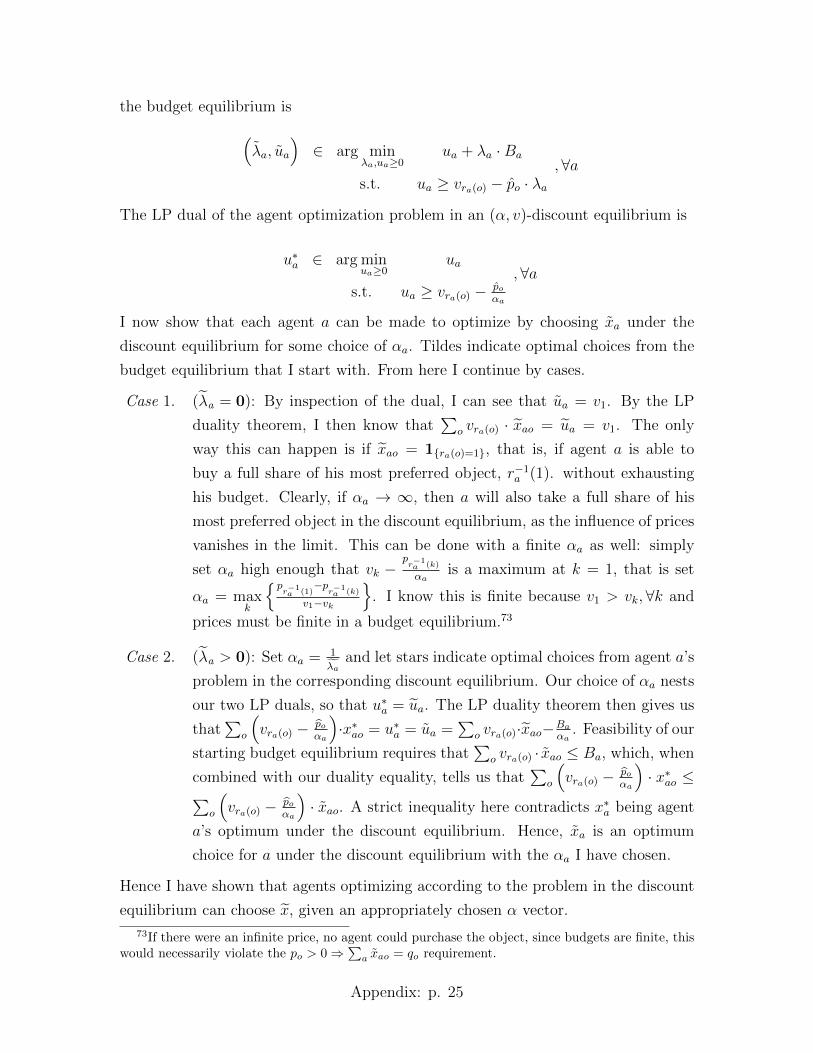
the budget equilibrium is(λa, ua

)∈ arg min

λa,ua≥0ua + λa ·Ba

s.t. ua ≥ vra(o) − po · λa,∀a

The LP dual of the agent optimization problem in an (α, v)-discount equilibrium is

u∗a ∈ arg minua≥0

ua

s.t. ua ≥ vra(o) − poαa

,∀a

I now show that each agent a can be made to optimize by choosing xa under the

discount equilibrium for some choice of αa. Tildes indicate optimal choices from the

budget equilibrium that I start with. From here I continue by cases.

Case 1. (λa = 0): By inspection of the dual, I can see that ua = v1. By the LP

duality theorem, I then know that∑

o vra(o) · xao = ua = v1. The only

way this can happen is if xao = 1ra(o)=1, that is, if agent a is able to

buy a full share of his most preferred object, r−1a (1). without exhausting

his budget. Clearly, if αa → ∞, then a will also take a full share of his

most preferred object in the discount equilibrium, as the influence of prices

vanishes in the limit. This can be done with a finite αa as well: simply

set αa high enough that vk −pr−1a (k)

αais a maximum at k = 1, that is set

αa = maxk

pr−1a (1)

−pr−1a (k)

v1−vk

. I know this is finite because v1 > vk,∀k and

prices must be finite in a budget equilibrium.73

Case 2. (λa > 0): Set αa = 1

λaand let stars indicate optimal choices from agent a’s

problem in the corresponding discount equilibrium. Our choice of αa nests

our two LP duals, so that u∗a = ua. The LP duality theorem then gives us

that∑

o

(vra(o) − po

αa

)·x∗ao = u∗a = ua =

∑o vra(o)·xao−Ba

αa. Feasibility of our

starting budget equilibrium requires that∑

o vra(o) · xao ≤ Ba, which, when

combined with our duality equality, tells us that∑

o

(vra(o) − po

αa

)· x∗ao ≤∑

o

(vra(o) − po

αa

)· xao. A strict inequality here contradicts x∗a being agent

a’s optimum under the discount equilibrium. Hence, xa is an optimum

choice for a under the discount equilibrium with the αa I have chosen.

Hence I have shown that agents optimizing according to the problem in the discount

equilibrium can choose x, given an appropriately chosen α vector.

73If there were an infinite price, no agent could purchase the object, since budgets are finite, thiswould necessarily violate the po > 0⇒

∑a xao = qo requirement.

Appendix: p. 25

Theorem 7. x is supportably rank efficient if and only if there exist budgets and a

valuation, (B, v), such that x is supported by the (B, v)-budget mechanism.

Proof. The previous two proofs establish the result.

The efficiency of the budget equilibria lines up well with a textbook understanding

of general equilibrium and the welfare theorems, but it is less clear why the discount

equilibrium should yield an efficient outcome, as distorting prices with the α-discounts

seems like it should cause trouble in the same way that distortionary taxation does.

So what is going on? The agent’s problem in the discount equilibrium can be thought

of as the problem of an agent with enough money to buy whatever he wants, but who

values money quasi-linearly. In the artificial economy where money factors into the

agent’s utility, the discount equilibrium will not be efficient. The efficiency concepts

in this paper, however, ignore the artificial money and rely only on the distribution

of objects among the agents. In short, in the discount equilibrium, distortions in

the relative cost of keeping money serve a similar role to the budgets in the budget

equilibrium, but they do so in a way that allows more precise control over what Pareto

weights will support the chosen optimal assignment (at the cost of sacrificing control

over agents’ opportunity sets).

Appendix: p. 26