range reference atmosphere 2019 - nasa
TRANSCRIPT
1
Range Reference Atmosphere 2019
Lee Burns, Ph.D.
Jacobs SEG
JPID-FY19-001801
1
TABLE OF CONTENTS
1.0 INTRODUCTION
1.1 Definition of a Range Reference Atmosphere
1.2 Purpose
1.3 History
1.4 Scope, Contents, and Arrangement of Data Tables
2.0 METHODOLOGY OVERVIEW
3.0 STEP 1: DEFINE/OBTAIN/INITIALIZE INPUT DATA
4.0 STEP 2: PERFORM QUALITY CONTROL
4.1 Out of Bounds Value Check
4.2 Surface level Check
4.3 Duplicate Profile Check
4.4 Missing Data Check
4.5 Minimum Number of Valid Data Levels Check
4.6 Maximum Data Gap Interval Check
4.7 Wind Speed Shear Check
4.8 Negative Delta-Z Check
4.9 Visual Inspection Check Based on Subject Matter Expertise
5.0 STEP 3: INTERPOLATE PROFILE DATA
5.1 Establish Output Altitude Grid
5.2 Compute Geopotential Heights for Output Grid Altitudes
5.2.1 Compute Latitude-Dependent Surface Gravity
5.2.2 Compute Vertical Derivative of Gravity at Surface
5.2.3 Compute Effective Earth Radius
5.2.4 Compute Geopotential Heights
5.3 Compute Wind Components
5.4 Interpolate Wind Speed and Wind Components to Output Grid
5.5 Interpolate Pressure to Output Grid
5.6 Interpolate Temperature and Dewpoint to Output Grid
6.0 STEP 4: COMPUTE DERIVED QUANTITIES
6.1 Compute Vapor Pressure
6.2 Compute Virtual Temperature
6.3 Compute Density
7.0 STEP 5: COMPUTE STATISTICS
8.0 STEP 6: PERFORM DIAGNOSTIC TESTING

2
9.0 STEP 7: PERFORM VALIDATION TESTING
9.1 Skewness Limit Tests
9.2 Buell Relationship Tests
9.3 Gas Law Reconstruction Test
9.4 Wind Speed Reconstruction Test
10.0 STEP 8: CREATE FINAL DATA PRODUCTS
REFFERENCES
3
1.0 INTRODUCTION
1.1 Definition of a Range Reference Atmosphere
A reference atmosphere is a statistical description of the Earth’s atmosphere derived from upper-
air measurements over some geographical area. Typically, reference atmospheres provide mean
values and some measures of variability for a number of atmospheric state variables, such as
pressure, density, temperature, wind speed, etc. The first reference atmosphere, developed in the
1920’s [1], was referred to as a “standard atmosphere.” Standard atmospheres are intended to be
applicable over large spatial domains (mid-latitudes, for example). For higher-fidelity
characterization of the atmosphere at a particular location, site-specific reference atmospheres
were later developed. This type of reference atmosphere is referred to as a Range Reference
Atmosphere (RRA). RRAs are, formally, a product of the Range Commander’s Council (RCC)
Meteorology Group (RCC-MG). The Marshall Space Flight Center (MSFC) Natural
Environments (NE) Branch has developed a new series of RRAs on behalf of the RCC-MG. This
document details the development methodology and the results obtained for the 2019 RRAs.
1.2 Purpose
A series of revised and expanded RRAs are to be published for locations of interest to the RCC.
These datasets will serve as authoritative reference sources on certain upper air statistics and as
atmospheric models for their respective range sites (locations). The technical usefulness of these
documents for the ranges, range users, U.S. aerospace industries, and the scientific community is
recognized because of the standardization of the development techniques and the presentation of
the tabulations.
1.3 History
Many RRAs have been produced over the years. The Inter-Range Instrumentation Group
Meteorology Working Group (IRIG-MWG), the organizational predecessor to the RCC-MG,
published several RRAs from 1963 through 1974. Beginning in 1983, the RCC-MG published a
new updated series of RRAs (RRA version 1983) to take advantage of improved measurement
systems and data processing capabilities [2]. A standardized process was implemented to generate
this series of RRAs, in contrast to previous versions, which were generated using non-
standardized, site-specific methodologies. Beginning in 2002, a second series of RRA updates
was generated by the Air Force Combat Climatology Center (now known as the 14th Weather
Squadron) [3]. These datasets were published by the RCC-MG in 2006 (RRA version 2006).
Beginning in 2013, MSFC NE produced a third series of RRA updates (RRA version 2013). The
RCC-MG intends to produce new RRA versions quasi-periodically to maintain the best possible
current representations of the upper atmospheres (surface to 30 km altitude) at selected ranges of
interest. In 2018, MSFC-NE agreed to develop a fourth series of RRA updates, resulting in the
current document and associated data tables. These new datasets will be referred to as RRA
version 2019.
4
1.4 Scope, Contents, and Arrangement of Data Tables
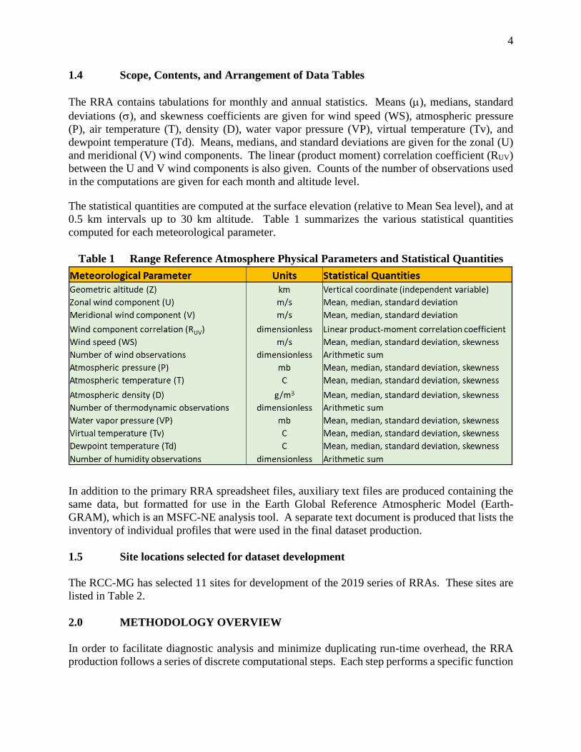
The RRA contains tabulations for monthly and annual statistics. Means (), medians, standard
deviations (), and skewness coefficients are given for wind speed (WS), atmospheric pressure
(P), air temperature (T), density (D), water vapor pressure (VP), virtual temperature (Tv), and
dewpoint temperature (Td). Means, medians, and standard deviations are given for the zonal (U)
and meridional (V) wind components. The linear (product moment) correlation coefficient (RUV)
between the U and V wind components is also given. Counts of the number of observations used
in the computations are given for each month and altitude level.
The statistical quantities are computed at the surface elevation (relative to Mean Sea level), and at
0.5 km intervals up to 30 km altitude. Table 1 summarizes the various statistical quantities
computed for each meteorological parameter.
Table 1 Range Reference Atmosphere Physical Parameters and Statistical Quantities
In addition to the primary RRA spreadsheet files, auxiliary text files are produced containing the
same data, but formatted for use in the Earth Global Reference Atmospheric Model (Earth-
GRAM), which is an MSFC-NE analysis tool. A separate text document is produced that lists the
inventory of individual profiles that were used in the final dataset production.
1.5 Site locations selected for dataset development
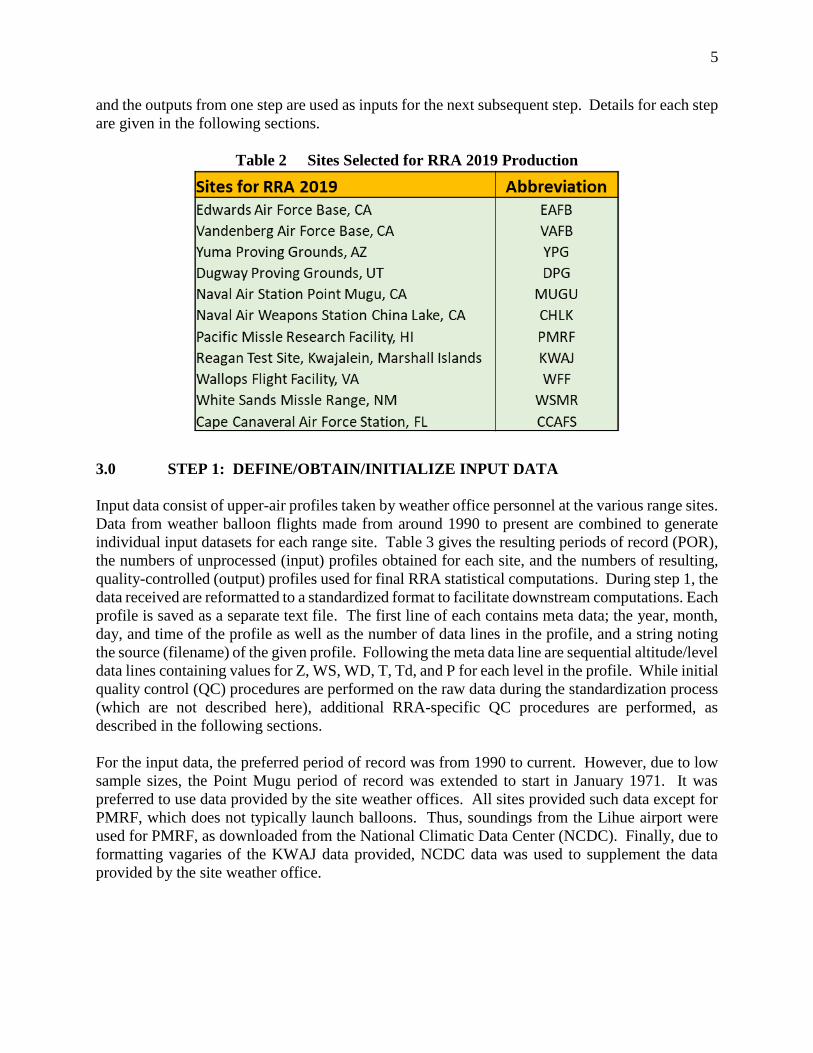
The RCC-MG has selected 11 sites for development of the 2019 series of RRAs. These sites are
listed in Table 2.
2.0 METHODOLOGY OVERVIEW
In order to facilitate diagnostic analysis and minimize duplicating run-time overhead, the RRA
production follows a series of discrete computational steps. Each step performs a specific function
5
and the outputs from one step are used as inputs for the next subsequent step. Details for each step
are given in the following sections.
Table 2 Sites Selected for RRA 2019 Production
3.0 STEP 1: DEFINE/OBTAIN/INITIALIZE INPUT DATA
Input data consist of upper-air profiles taken by weather office personnel at the various range sites.
Data from weather balloon flights made from around 1990 to present are combined to generate
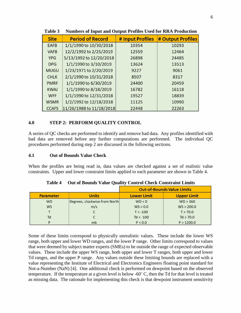
individual input datasets for each range site. Table 3 gives the resulting periods of record (POR),
the numbers of unprocessed (input) profiles obtained for each site, and the numbers of resulting,
quality-controlled (output) profiles used for final RRA statistical computations. During step 1, the
data received are reformatted to a standardized format to facilitate downstream computations. Each
profile is saved as a separate text file. The first line of each contains meta data; the year, month,
day, and time of the profile as well as the number of data lines in the profile, and a string noting
the source (filename) of the given profile. Following the meta data line are sequential altitude/level
data lines containing values for Z, WS, WD, T, Td, and P for each level in the profile. While initial
quality control (QC) procedures are performed on the raw data during the standardization process
(which are not described here), additional RRA-specific QC procedures are performed, as
described in the following sections.
For the input data, the preferred period of record was from 1990 to current. However, due to low
sample sizes, the Point Mugu period of record was extended to start in January 1971. It was
preferred to use data provided by the site weather offices. All sites provided such data except for
PMRF, which does not typically launch balloons. Thus, soundings from the Lihue airport were
used for PMRF, as downloaded from the National Climatic Data Center (NCDC). Finally, due to
formatting vagaries of the KWAJ data provided, NCDC data was used to supplement the data
provided by the site weather office.
6
Table 3 Numbers of Input and Output Profiles Used for RRA Production
4.0 STEP 2: PERFORM QUALITY CONTROL
A series of QC checks are performed to identify and remove bad data. Any profiles identified with
bad data are removed before any further computations are performed. The individual QC
procedures performed during step 2 are discussed in the following sections.
4.1 Out of Bounds Value Check
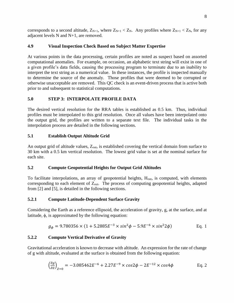
When the profiles are being read in, data values are checked against a set of realistic value
constraints. Upper and lower constraint limits applied to each parameter are shown in Table 4.
Table 4 Out of Bounds Value Quality Control Check Constraint Limits
Some of these limits correspond to physically unrealistic values. These include the lower WS
range, both upper and lower WD ranges, and the lower P range. Other limits correspond to values
that were deemed by subject matter experts (SMEs) to be outside the range of expected observable
values. These include the upper WS range, both upper and lower T ranges, both upper and lower
Td ranges, and the upper P range. Any values outside these limiting bounds are replaced with a
value representing the Institute of Electrical and Electronics Engineers floating point standard for
Not-a-Number (NaN) [4]. One additional check is performed on dewpoint based on the observed
temperature. If the temperature at a given level is below -60˚ C, then the Td for that level is treated
as missing data. The rationale for implementing this check is that dewpoint instrument sensitivity
7
decreases rapidly for temperatures below -60˚ C. At these temperatures, it is reasonable to assume
that the moisture content in the air is negligible.
4.2 Surface level Check
Profiles are required to start with valid data values within 0.1 km of the nominal surface elevation
for each site. Any profile with a lowest reporting altitude above this limit is removed.
4.3 Duplicate Profile Check
Occasionally, data from the same balloon flight are represented in the archive at multiple vertical
resolutions. For example, a given profile may be present in both 100 ft and 1000 ft resolutions.
When data from a given balloon flight exist in multiple resolutions, only the data with the lowest
resolution are retained.
4.4 Missing Data Check
Various “missing data” flags (for example, -999.99) are occasionally present in the data archive in
place of valid data entries. Any missing data flags are replaced with NaN.
4.5 Minimum Number of Valid Data Levels Check
A test is performed to ensure that each input profile contains at least five levels with valid data
values. This test is performed independently for the parameters WS, T, Td, and P. Any profile
containing less than five levels with valid observations of WS, T, Td, or P are removed. Note that
this QC check does not require a profile to have at least five levels containing valid observations
of all test parameters simultaneously at that same level.
4.6 Maximum Data Gap Interval Check
A test is performed to ensure that no data gaps larger than 5 km were present. Any profiles with
data gaps (altitude differences between adjacent levels with valid data values) larger than 5 km are
removed. This test is performed sequentially for WS, T, Td, and P.
4.7 Wind Speed Shear Check
A maximum wind shear limit is established with a value of 0.3 s-1. Any profile containing wind
speed shears between adjacent data reporting levels that exceeded the established limit is removed.
4.8 Negative Altitude Change Between Adjacent Levels Check
Occasionally a profile is noted to be corrupt as though portions of two separate profiles are written
on a single line. Typically, this is manifested as a profile that appears valid up to some given level,
after which the profile data is over-written by a second full profile. In these instances, the given,
Nth data level corresponds to a given altitude, say ZN, while the next subsequent, (N+1)th data level
8
corresponds to a second altitude, ZN+1, where ZN+1 < ZN. Any profiles where ZN+1 < ZN, for any
adjacent levels N and N+1, are removed.
4.9 Visual Inspection Check Based on Subject Matter Expertise
At various points in the data processing, certain profiles are noted as suspect based on assorted
computational anomalies. For example, on occasion, an alphabetic text string will exist in one of
a given profile’s data fields, causing the processing program to terminate due to an inability to
interpret the text string as a numerical value. In these instances, the profile is inspected manually
to determine the source of the anomaly. Those profiles that were deemed to be corrupted or
otherwise unacceptable are removed. This QC check is an event-driven process that is active both
prior to and subsequent to statistical computations.
5.0 STEP 3: INTERPOLATE PROFILE DATA
The desired vertical resolution for the RRA tables is established as 0.5 km. Thus, individual
profiles must be interpolated to this grid resolution. Once all values have been interpolated onto
the output grid, the profiles are written to a separate text file. The individual tasks in the
interpolation process are detailed in the following sections.
5.1 Establish Output Altitude Grid
An output grid of altitude values, Zout, is established covering the vertical domain from surface to
30 km with a 0.5 km vertical resolution. The lowest grid value is set at the nominal surface for
each site.
5.2 Compute Geopotential Heights for Output Grid Altitudes
To facilitate interpolations, an array of geopotential heights, Hout, is computed, with elements
corresponding to each element of Zout. The process of computing geopotential heights, adapted
from [2] and [5], is detailed in the following sections.
5.2.1 Compute Latitude-Dependent Surface Gravity
Considering the Earth as a reference ellipsoid, the acceleration of gravity, g, at the surface, and at
latitude, , is approximated by the following equation:
𝑔𝜙 = 9.780356 × (1 + 5.2885𝐸−3 × 𝑠𝑖𝑛2𝜙 − 5.9𝐸−6 × 𝑠𝑖𝑛22𝜙) Eq. 1
5.2.2 Compute Vertical Derivative of Gravity
Gravitational acceleration is known to decrease with altitude. An expression for the rate of change
of g with altitude, evaluated at the surface is obtained from the following equation:
(𝜕𝑔
𝜕𝑍)
𝑍=0= −3.085462𝐸−6 + 2.27𝐸−9 × 𝑐𝑜𝑠2𝜙 − 2𝐸−12 × 𝑐𝑜𝑠4𝜙 Eq. 2
9
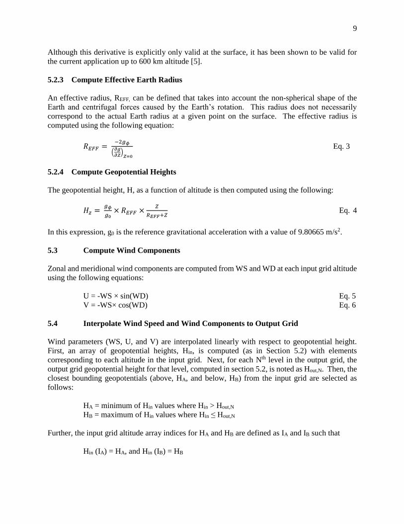
Although this derivative is explicitly only valid at the surface, it has been shown to be valid for
the current application up to 600 km altitude [5].
5.2.3 Compute Effective Earth Radius
An effective radius, REFF, can be defined that takes into account the non-spherical shape of the
Earth and centrifugal forces caused by the Earth’s rotation. This radius does not necessarily
correspond to the actual Earth radius at a given point on the surface. The effective radius is
computed using the following equation:
𝑅𝐸𝐹𝐹 = −2𝑔𝜙
(𝜕𝑔
𝜕𝑍)
𝑍=0
Eq. 3
5.2.4 Compute Geopotential Heights
The geopotential height, H, as a function of altitude is then computed using the following:
𝐻𝑧 = 𝑔𝜙
𝑔0× 𝑅𝐸𝐹𝐹 ×
𝑍
𝑅𝐸𝐹𝐹+𝑍 Eq. 4
In this expression, g0 is the reference gravitational acceleration with a value of 9.80665 m/s2.
5.3 Compute Wind Components
Zonal and meridional wind components are computed from WS and WD at each input grid altitude
using the following equations:
U = -WS × sin(WD) Eq. 5
V = -WS× cos(WD) Eq. 6
5.4 Interpolate Wind Speed and Wind Components to Output Grid
Wind parameters (WS, U, and V) are interpolated linearly with respect to geopotential height.
First, an array of geopotential heights, Hin, is computed (as in Section 5.2) with elements
corresponding to each altitude in the input grid. Next, for each Nth level in the output grid, the
output grid geopotential height for that level, computed in section 5.2, is noted as Hout,N. Then, the
closest bounding geopotentials (above, HA, and below, HB) from the input grid are selected as
follows:
HA = minimum of Hin values where Hin > Hout,N
HB = maximum of Hin values where Hin ≤ Hout,N
Further, the input grid altitude array indices for HA and HB are defined as IA and IB such that
Hin (IA) = HA, and Hin (IB) = HB
10
Then, upper and lower input grid values for WS, U, and V are determined as the array elements
defined by the indices IA and IB:
WSA = WS(IA)
WSB = WS(IB)
UA = U(IA)
UB = U(IB)
VA = V(IA)
VB = V(IB)
Now, a term, C1, can be defined where C1 = (Hout,N – HB)/(HA – HB). Then, the Nth interpolated
values for WS, U, and V are computed:
WSN = WSB + (WSA – WSB) * C1 Eq. 7
UN = UB + (UA – UB) * C1 Eq. 8
VN = VB + (VA – VB) * C1 Eq. 9
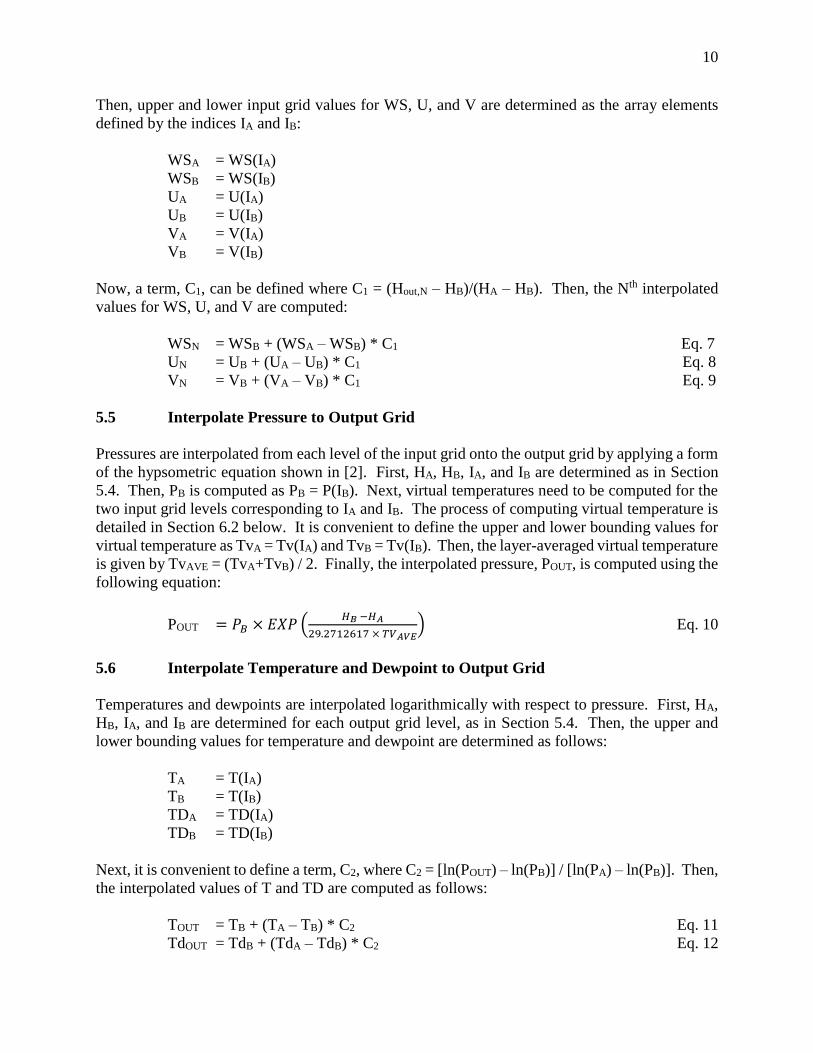
5.5 Interpolate Pressure to Output Grid
Pressures are interpolated from each level of the input grid onto the output grid by applying a form
of the hypsometric equation shown in [2]. First, HA, HB, IA, and IB are determined as in Section
5.4. Then, PB is computed as PB = P(IB). Next, virtual temperatures need to be computed for the
two input grid levels corresponding to IA and IB. The process of computing virtual temperature is
detailed in Section 6.2 below. It is convenient to define the upper and lower bounding values for
virtual temperature as TvA = Tv(IA) and TvB = Tv(IB). Then, the layer-averaged virtual temperature
is given by TvAVE = (TvA+TvB) / 2. Finally, the interpolated pressure, POUT, is computed using the
following equation:
POUT = 𝑃𝐵 × 𝐸𝑋𝑃 (𝐻𝐵 −𝐻𝐴
29.2712617 × 𝑇𝑉𝐴𝑉𝐸) Eq. 10
5.6 Interpolate Temperature and Dewpoint to Output Grid
Temperatures and dewpoints are interpolated logarithmically with respect to pressure. First, HA,
HB, IA, and IB are determined for each output grid level, as in Section 5.4. Then, the upper and
lower bounding values for temperature and dewpoint are determined as follows:
TA = T(IA)
TB = T(IB)
TDA = TD(IA)
TDB = TD(IB)
Next, it is convenient to define a term, C2, where C2 = [ln(POUT) – ln(PB)] / [ln(PA) – ln(PB)]. Then,
the interpolated values of T and TD are computed as follows:
TOUT = TB + (TA – TB) * C2 Eq. 11
TdOUT = TdB + (TdA – TdB) * C2 Eq. 12
11
6.0 STEP 4: COMPUTE DERIVED QUANTITIES
Once all profiles of WS, U, V, T, Td, and P have been interpolated to the output grid resolution,
values for the additional derived quantities of VP, Tv, and D are computed as shown in the
following sections. These equations and methods are adapted from [2].
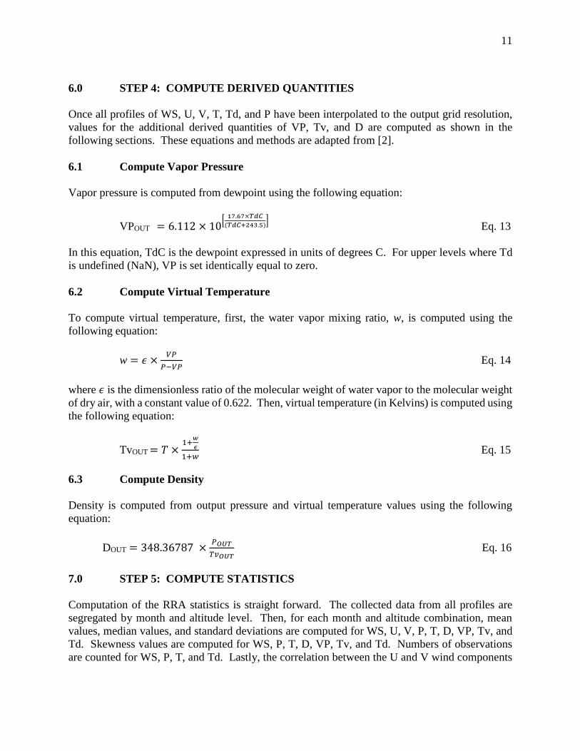
6.1 Compute Vapor Pressure
Vapor pressure is computed from dewpoint using the following equation:
VPOUT = 6.112 × 10[
17.67×𝑇𝑑𝐶
(𝑇𝑑𝐶+243.5)] Eq. 13
In this equation, TdC is the dewpoint expressed in units of degrees C. For upper levels where Td
is undefined (NaN), VP is set identically equal to zero.
6.2 Compute Virtual Temperature
To compute virtual temperature, first, the water vapor mixing ratio, w, is computed using the
following equation:
w = 𝜖 ×𝑉𝑃
𝑃−𝑉𝑃 Eq. 14
where 𝜖 is the dimensionless ratio of the molecular weight of water vapor to the molecular weight
of dry air, with a constant value of 0.622. Then, virtual temperature (in Kelvins) is computed using
the following equation:
TvOUT = 𝑇 ×1+
𝑤
𝜖
1+𝑤 Eq. 15
6.3 Compute Density
Density is computed from output pressure and virtual temperature values using the following
equation:
DOUT = 348.36787 ×𝑃𝑂𝑈𝑇
𝑇𝑣𝑂𝑈𝑇 Eq. 16
7.0 STEP 5: COMPUTE STATISTICS
Computation of the RRA statistics is straight forward. The collected data from all profiles are
segregated by month and altitude level. Then, for each month and altitude combination, mean
values, median values, and standard deviations are computed for WS, U, V, P, T, D, VP, Tv, and
Td. Skewness values are computed for WS, P, T, D, VP, Tv, and Td. Numbers of observations
are counted for WS, P, T, and Td. Lastly, the correlation between the U and V wind components
12
is calculated. Data values of NaN are not used in these computations. All computed values are
tabulated in an intermediate output file.
8.0 STEP 6: PERFORM DIAGNOSTIC TESTING
Diagnostic testing is performed individually for the variables WS, U, V, T, P, and Td. After
computing monthly mean values and standard deviations at each RRA altitude, all profiles of a
given variable for a given month are plotted together along with the +/- 6 envelopes. All
profiles with values that exceeded the envelope limits at any level are flagged for removal.
After removing these flagged profiles, step 5 is repeated to give a new set of RRA statistics. Then,
step 6 is repeated with new envelopes derived from the new means and standard deviations. Steps
5 and 6 are iterated until no profiles exceed any of the +/- 6 envelopes.
9.0 STEP 7: PERFORM VALIDATION TESTING
Once a set of RRA statistics successfully passes the diagnostic testing process, an additional series
of tests are performed to establish the validity of the statistical values. The individual tests are
described in detail in the following sections. Some of these tests have quantified success criteria
while others require SME judgment to determine pass/fail conditions. It should be noted that a
failure of one of these validation tests does not suggest a clear remediation process. For example,
no individual profiles are indicated as the cause of the failure condition. Rather, these tests were
used to indicate the presence of some problem. Once detected, the problem is addressed through
in-depth manual inspection of the input data and various idiomatic analyses of the constituent data
values. Any erroneous profiles discovered to be supporting the failure condition are removed from
the input database and the development process is repeated beginning with step 5. This process is
iterated until no validation test failures are noted.
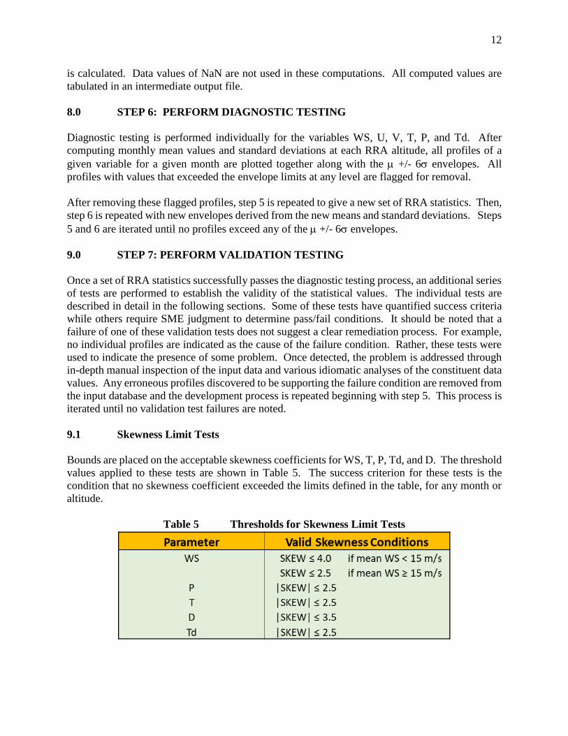
9.1 Skewness Limit Tests
Bounds are placed on the acceptable skewness coefficients for WS, T, P, Td, and D. The threshold
values applied to these tests are shown in Table 5. The success criterion for these tests is the
condition that no skewness coefficient exceeded the limits defined in the table, for any month or
altitude.
Table 5 Thresholds for Skewness Limit Tests
13
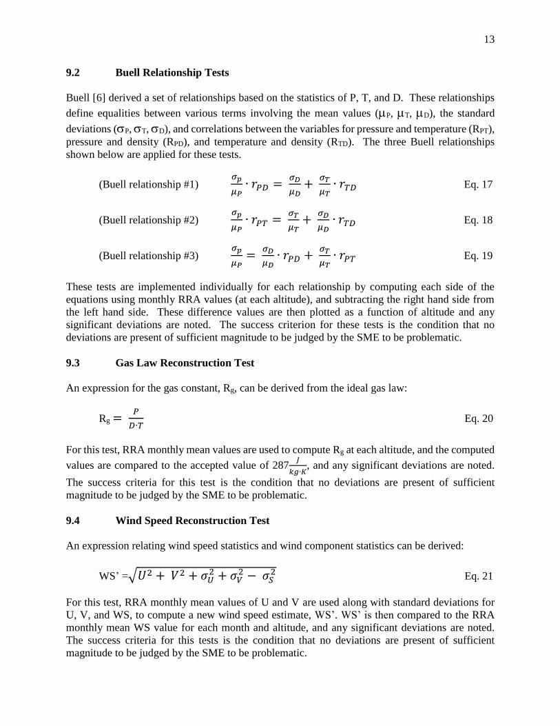
9.2 Buell Relationship Tests
Buell [6] derived a set of relationships based on the statistics of P, T, and D. These relationships
define equalities between various terms involving the mean values (P, T, D), the standard
deviations (P, T, D), and correlations between the variables for pressure and temperature (RPT),
pressure and density (RPD), and temperature and density (RTD). The three Buell relationships
shown below are applied for these tests.
(Buell relationship #1) 𝜎𝑝
𝜇𝑃∙ 𝑟𝑃𝐷 =
𝜎𝐷
𝜇𝐷+
𝜎𝑇
𝜇𝑇∙ 𝑟𝑇𝐷 Eq. 17
(Buell relationship #2) 𝜎𝑝
𝜇𝑃∙ 𝑟𝑃𝑇 =
𝜎𝑇
𝜇𝑇+
𝜎𝐷
𝜇𝐷∙ 𝑟𝑇𝐷 Eq. 18
(Buell relationship #3) 𝜎𝑝
𝜇𝑃=
𝜎𝐷
𝜇𝐷∙ 𝑟𝑃𝐷 +
𝜎𝑇
𝜇𝑇∙ 𝑟𝑃𝑇 Eq. 19
These tests are implemented individually for each relationship by computing each side of the
equations using monthly RRA values (at each altitude), and subtracting the right hand side from
the left hand side. These difference values are then plotted as a function of altitude and any
significant deviations are noted. The success criterion for these tests is the condition that no
deviations are present of sufficient magnitude to be judged by the SME to be problematic.
9.3 Gas Law Reconstruction Test
An expression for the gas constant, Rg, can be derived from the ideal gas law:
Rg = 𝑃
𝐷∙𝑇 Eq. 20
For this test, RRA monthly mean values are used to compute Rg at each altitude, and the computed
values are compared to the accepted value of 287𝐽
𝑘𝑔∙𝐾, and any significant deviations are noted.
The success criteria for this test is the condition that no deviations are present of sufficient
magnitude to be judged by the SME to be problematic.
9.4 Wind Speed Reconstruction Test
An expression relating wind speed statistics and wind component statistics can be derived:
WS’ =√𝑈2 + 𝑉2 + 𝜎𝑈2 + 𝜎𝑉
2 − 𝜎𝑆2 Eq. 21
For this test, RRA monthly mean values of U and V are used along with standard deviations for
U, V, and WS, to compute a new wind speed estimate, WS’. WS’ is then compared to the RRA
monthly mean WS value for each month and altitude, and any significant deviations are noted.
The success criteria for this tests is the condition that no deviations are present of sufficient
magnitude to be judged by the SME to be problematic.
14
10.0 STEP 8: CREATE FINAL DATA PRODUCTS
Once all issues identified in validation testing are successfully addressed and a set of RRA statistics
are generated that pass all validation tests, the following final data products are created: (1) a
Comma Separated Variable Excel spreadsheet file containing computed RRA values for all
statistical parameters for all months and altitudes, (2) an Earth-GRAM formatted text file
containing wind statistics, (3) an Earth-GRAM formatted text file containing thermodynamic
statistics, (4) an Earth-GRAM formatted text file containing moisture statistics, and (5) a listing,
by timestamp, of the constituent profiles used to produce the final RRA product.
15
REFERENCES
[1] Kyle, T. G., Atmospheric Transmission, Emission, and Scattering, Pergamon
Press, New York, NY, 1991
[2] Range Commanders Council Meteorological Group, Cape Canaveral Florida
Range Reference Atmosphere 0-70 km Altitude, Range Commanders Council
Secretariat, White Sands Missile Range, NM, 1983.
[3] "Range Reference Atmosphere Climatologies," Edwards Air Force Base Weather
Office, Updated 2013, <https://bsx.edwards.af.mil/weather/wxclimatology.htm>.
[4] Institute of Electrical and Electronics Engineers, IEEE Standard for Floating-
Point Arithmetic, IEEE Standard 754-2008, IEEE Publishing, New York, NY,
2008.
[5] List, R. J., Smithsonian Meteorological Tables, Smithsonian Institute Press,
Washington, DC. 1951.
[6] Buell, C. E., “Some Relations Among Atmospheric Statistics,” J. Meteor., 11,
pp. 238-254.