RAMS/BRAMSBasic equations

and some numerical issues

General equations

• The equations are the standard non-hydrostatic Reynolds-averaged primitive equations.

• AlI variables, unless otherwise denoted, are grid-volume averaged quantities where the overbar has been omitted.

• The horizontal and vertical grid transformations (described later) are omitted for clarity.

Equations of motion:

Thermodynamic equation:

+ PR(Θil)

Water species mixing ratio continuity equation:

+ Sn

Mass continuity equation:

T

cp

pc p

cR

p

p

d

00

Exner function

3D domain :“box grids”

x, y, z -– grid spacing

Grid structure

• standard C grid (Mesinger and Arakawa, 1976). • alI thermodynamic and moisture variables

are defined at the same point • with the velocity components u,v, and w staggered

1/2 Δx, 1/2 Δy, and 1/2 Δz respectively.

Grid stagger

Δz

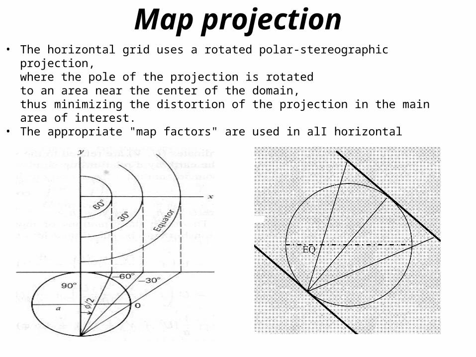
Map projection• The horizontal grid uses a rotated polar-stereographic projection,

where the pole of the projection is rotated to an area near the center of the domain,

thus minimizing the distortion of the projection in the main area of interest.

• The appropriate "map factors" are used in alI horizontal derivative terms.

Sp

p

Philips (1957) : “sigma”

0 1

vertical coordinate system

Terrain-following coordinate• The vertical structure of the grid uses the σz

terrain-following coordinate system • It is a terrain-following coordinate system where

the top of the model domain is exactly flat and the bottom follows the terrain.

• The coordinates in this system are defined as:

H – height of the top of the grid

Zg – local topography height

• Derivative terms can be written in tensor notation as:

• and the tensor bij is written as:

The relationship between the Cartesian wind components and the components in the transformed system is:

•This transformation can be viewed as a simple mapping of the horizontal velocity components to the terrain-following system since they

remain horizontal in Cartesian space. • This eliminates the complication of dealing with non-orthogonal velocity

components. • The vertical component, w*, has an imposed value of zero at z*, which implies no mass flux through the ground surface.

Time differencing

• the time differencing scheme is a hybrid scheme which consists of forward time differencing for the thermodynamic variables and leapfrog differencing for the velocity components and pressure.

"time-split" Time differencing• The basic idea behind these schemes is to "split" off in a series of smaller

time steps those terms in the equation that are responsible for the propagation of the fast wave modes (acoustic and gravity waves)

• The time differencing schemes can be demonstrated as follows for simplified two-dimensional, dry, inviscid, quasi-Boussinesq equation sets where the vertical and horizontal coordinate transformations have been removed for

where c is the speed of sound.

• The computational procedure is then as follows for a forward-backward time differencing scheme:

1. The right hand side of [22] and [24], Fu, Fw, and Fθ are computed.

2. The velocity components are stepped to t + Δts

3. Pressure at t + Δts, is computed with [25], using the newly updated velocity components at t + Δts

4. The small time step is repeated n times until n Δts = ΔtL.

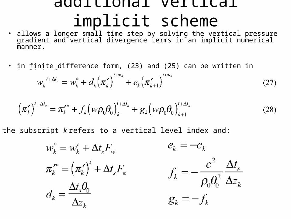
additional vertical implicit scheme• allows a longer small time step by solving the vertical pressure gradient

and vertical divergence terms in an implicit numerical manner.

• in finite difference form, (23) and (25) can be written in implicit form as:

where the subscript k refers to a vertical level index and:

• Equation (30) can be easily solved with a tri-diagonal matrix technique.

• These results for w*k would then be used in (25) to solve for to complete the small time step.

• Substituting (28) into (27) and rearranging yields:

where

other considerations :• inclusion of a Crank-Nicholson scheme in the matrix solution.• also contains a modification of c, the speed of sound, to allow a longer small time step lowers c in (25).• Reduction of c by a factor between .4 and 1 usually has no significanteffect on the model solution.

Advection• two types of advection schemes:

standard leapfrog-type schemes (velocity components)forward-upstream schemes (scalar variables)

• The advective schemes are configured in flux form in order to conserve mass and momentum.

• Considering the x-direction, assuming constant grid spacing and omitting topographical and spherical transformations for clarity,

• the advective terms in (1)-(4) then can be generically written as:

where u is the wind component in the x direction, ρ is the air density, and Φ the variable to be advected. The subscript references a particular grid point.

advection fluxes

• Second-order leapfrog fluxes:

• Second-order forward fluxes:

(where α =u Δt / Δ x) :

Parallelism