rajshahi university journal - university of rajshahi
TRANSCRIPT
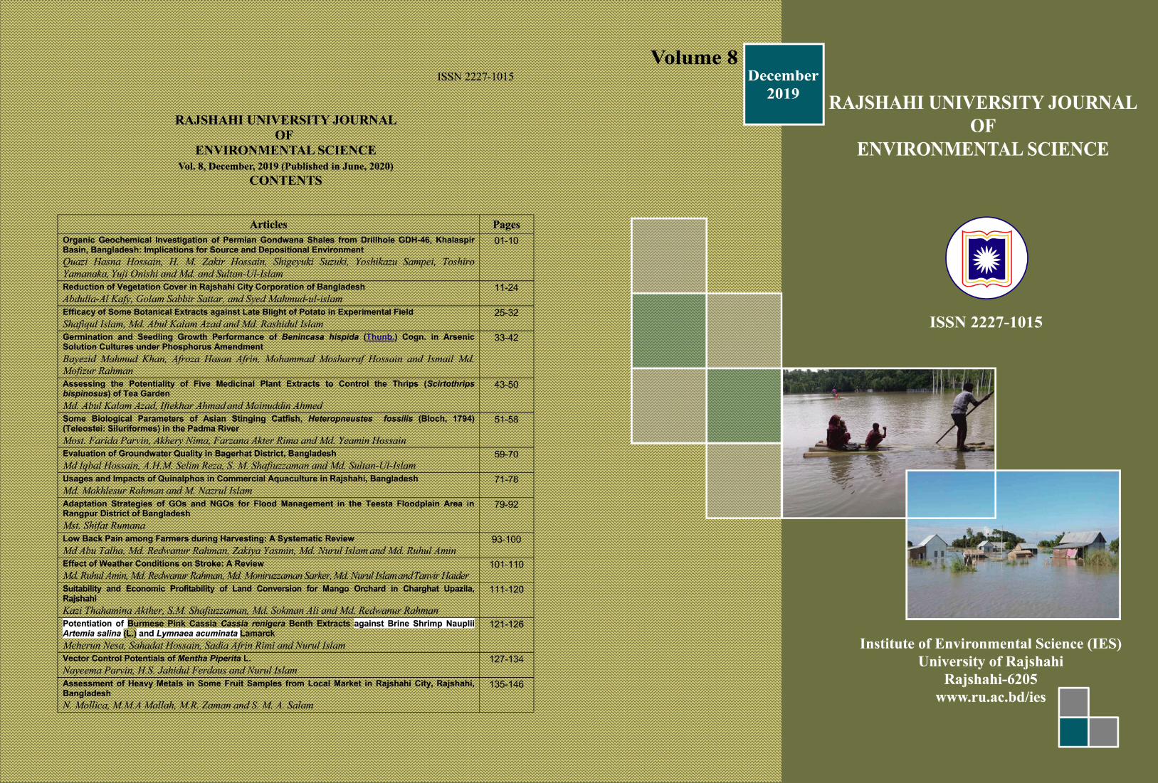
RAJSHAHI UNIVERSITY JOURNAL OF
ENVIRONMENTAL SCIENCE ISSN 2227-1015
Volume No. 8, December, 2019
(Published in June, 2020)
Published by
Institute of Environmental Science University of Rajshahi
Rajshahi-6205, Bangladesh www.ru.ac.bd/ies
@ All rights reserved by the publisher. The Journal is published annually accommodating all aspects of Environmental Science within available scope after peer review.
Subscriptions
Institutions: Inside Bangladesh Tk. 500 per copy Out side Bangladesh US$ 50 per copy Individual: Inside Bangladesh Tk. 300 per copy Out side Bangladesh US$ 30 per copy Correspondence: All correspondence should be addressed to the Chief Editor, Rajshahi University Journal of Environmental Science, Institute of Environmental Science, University of Rajshahi, Rajshahi-6205, Bangladesh. Website: www. ru.ac.bd/ies, E-mail: [email protected] and [email protected], Tel. 880-0721 750930
Cover Design: Prof. Dr. Md. Abul Kalam Azad Printed at: Uttoran Offset Printing Press, Greater Road, Rajshahi
ISSN 2227-1015
RAJSHAHI UNIVERSITY JOURNAL
OF ENVIRONMENTAL SCIENCE
An Annual Journal of the Institute of Environmental Science
Vol. No. 8, December, 2019
(Published in June, 2020)
EDITORIAL BOARD Chief Editor Prof. Dr. Md. Abul Kalam Azad Members Prof. Dr. Golam Sabbir Sattar Prof. Dr. Md. Golam Mostafa Prof. Dr. Md. Redwanur Rahman Prof. Dr. Jakir Hossain Prof. Dr. Md. Firoz Alam Prof. Dr. Sayed M A Salam Dr. S. M. Shafiuzzaman
Journal Liaison Officer: Md. Rajibul Hasan, Cell: 01712-002472 Published by: Institute of Environmental Science (IES), University of Rajshahi, Rajshahi-6205, Bangladesh E-mail: [email protected] and [email protected], website: www.ru.ac.bd/ies Phone: 880-0721-750930
FOREWORD
Conservation of environment is essential to ensure the security of water, food and energy for human beings. The challenges of environmental pollution, climate change and disasters must be addressed carefully with integrated initiatives, enhanced awareness and research. For deltaic landmass with vast coastal areas, the peoples of Bangladesh are the main sufferers of climate change and natural disasters. Therefore, interdisciplinary researches are utmost important for the control, mitigation, adaptation and dissemination of experiences for sustainable environmental management. The Rajshahi University Journal of Environmental Science (RUJES) is a multi-disciplinary journal to promote understanding of environmental issues includes environmental pollution, biodiversity loss, emission of carbon dioxide from fossil fuel, climate change and their impacts on air, water, soil and ecosystem. Thus, the journal offers a scientific platform for publishing the critical reviews and original research achievements through peer-review. All the contributors and reviewers are highly acknowledged for their interest, efforts and co-operation. I would like to express my sincere appreciation to the members of editorial board and associates for their support in publishing the current volume of the journal. I also thanks to the employees of printing press for their necessary help. Any further suggestion for the improvement of the next issues will be highly appreciated. The Chief Editor and Members of the Editorial Board do not bear any responsibility of the views expressed in the papers. The online version of the journal is available at: http://ru.ac.bd/ies Chief Editor
INSTRUCTIONS TO AUTHORS
Manuscripts: The manuscript must be sent in MS Word Document file format containing title of the paper, author's name(s), affiliation(s), author's full postal address and corresponding author’s e-mail. Abstract should be within 250 words along with maximum of 5 keywords indicating the objectives, results or conclusion of the study. The text of the full paper should preferably be within 5000 words (max. 10 pages) having the following sub-titles: o 1. Introduction: Introduction should be concise and precise relevant to objectives of study. o 2. Materials and Methods: Standard and published methods should not be described rather only be cited as
references. Any modification or new set up should be stated. o 3. Results and Discussion: Results should be presented with appropriate figures, tables, graphs, etc. with
proper interpretation and justification by relevant previous studies. o 4. Conclusion: Concise form of results with concluding remarks. o Tables, Graphs and Figures: The paper should contain maximum of 12 tables, graphs and figures all
together. Figures, graphs and photographs should be given as attached file along with appropriate marking numbers in standard BMP format (uncompressed). Original illustrator, graphic or photo files must be supplied with finally accepted manuscript.
o Acknowledgements (if any):
o References. Appropriate and relevant recent references must be cited following instruction given.
The following format needs to follow for preparation of manuscript: 1. Format Instructions
1.1. Instructions for Typists Margins are to be set to a width of 15.2 cm, and each page must be typed in Times New Roman 11 points letter for the main text with a 13 points spacing between the lines. The footnotes to be typed in Times New Roman 10 points letter with an 11 points spacing between the lines. Each page must be typed in a page depth of 21.6 cm. On the first page, the title of the paper should start after three blank lines below the journal heading. New paragraphs should be started without any indentation. Title of paper should be typed in bold, 14 point all upper-case letters, with 6 and 12 points spaces above and below respectively. The headings used are:
2. First-Order Heading These should be typed in bold, 12 point upper- and lower-case letters, with 6 points space above and below the heading. The text after the heading will begin at the left-hand margin (i.e., not indented as for new paragraph).
2.1. Second-Order Heading This should be typed in 12 point bold with a capital initial for each word at the left-hand margin, 6 points space above and below the heading.
2.1.1. Third-Order Heading This should be typed in 12 point bold with a capital initial for each word at the left-hand margin, 6 points space above and below the heading.
Special Attention
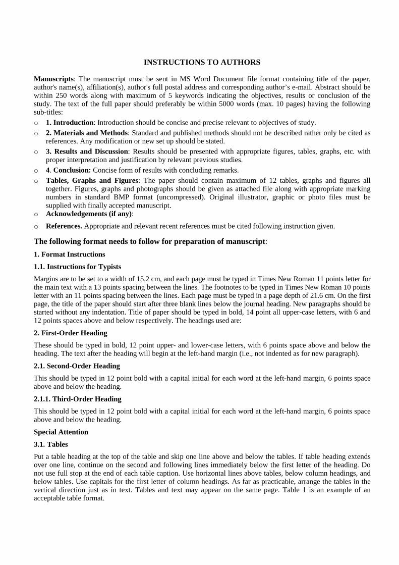
3.1. Tables Put a table heading at the top of the table and skip one line above and below the tables. If table heading extends over one line, continue on the second and following lines immediately below the first letter of the heading. Do not use full stop at the end of each table caption. Use horizontal lines above tables, below column headings, and below tables. Use capitals for the first letter of column headings. As far as practicable, arrange the tables in the vertical direction just as in text. Tables and text may appear on the same page. Table 1 is an example of an acceptable table format.
Table 1. Annual rainfall and water table of the study area
Areas
Annual Rainfall (mm) Water Table (m) Wet
Season Dry
Season Wet
Season Dry
Season Rajshahi Natore Pabna
20.4 30.6 45.9
27.4 38.6 46.9
90.0 34.6 45.0
20.4 31.6 43.9
3.2. Figures
Skip 6 points space above and below the figures. Put a figure caption at bottom of the figure and leave 6 points space between figure and caption, and use a full stop at end of the caption. Start second and subsequent lines immediately below the first letter of caption. Skip 6 points space after caption. Figures and text may appear on the same page. Legends, scales, etc. must be large enough to be legible. Give the consecutive numbers for tables and figures, respectively. You can break a paragraph for placing the figure. Try to avoid blank spaces within the text.
3.3. Equations
Equations should be numbered sequentially as follows: Use 1 line spacing instead of a 13 points spacing for the lines from just above to just below the equation. 02 =∇ φ (1)
3.4. References
In the text, author’s last name should be followed by the year of publication; e.g. “(Islam, 2016; Mostofa et al., 1997; Redwan and Shafiuzzaman, 2015) or “Azad (1998) showed that …”. In the list of references, arrange authors’ last names in alphabetical order with 0.5 cm indentation for the second and following lines of each reference. When two or more references by the same author are listed, the earlier work should appear first. All references must be cited in the text.
Style of References
For Journal:
Mostafa MG, Chen YH, Jean JS, Liu CC and Lee YC. 2011. Kinetics and Mechanism of Arsenate Removal by Nanosized Iron Oxide-coated Perlite. J. Hazardous Mat., 187: 89-95. Sen I, Parua DK, Bera S, Islam MS and Poole I. 2012. Contribution to the Neogene Fossil Wood Record and Palaeoecological Understanding of Bangladesh. Palaeontographica, Abteilung B: Palaophytologie, Palaeobotany-Palaeophytology, 288(1-4): 99-133.
For Book:
Blanford WT and Godwin-Austen HH. 1908. The Fauna of British India, including Ceylon and Burma, Mollusca: Testacellidae and Zonitidae: Taylor and Francis, London. 311p.
For Book Chapter:
Islam MB and Islam MS. 2006. Floods in Bangladesh: A Combined Interaction of Fluvio-anthropogenic Processes in the Sourse-sink Region, In: (Alphen JV, Beek EV and Taal M; eds): Floods, From Defence To Management. Taylor and Francis Group, London, England. P:589-595.
For Book Edited:
Kumar A and Bidhan D. 1989. A Text Book of Environmental Science (eds). (3rd edt) University Press, Dhaka, 525p.
For Dissertation/Thesis:
Mostafa MG. 2000. Thermodynamic Simulation of Cobalt-carbonate Aqueous System. PhD Dissertation (unpubl). Faculty of Engineering, Ehime University, Matsuyama, Japan, 200p.
For Report:
WDATCP (Wisconsin Department of Agriculture, Trade, and Consumer Protection). 1991. Report to the State Legislature: Agricultural Clean Sweep Demonstration Projects, Madison, WI: Agricultural Resource Management Division.
For Regulation:
USEPA (United States Environmental Protection Agency). 1995. Water Quality Standards-Revision of Metals Criteria, Fed. Reg., 60: 229-240.
For Proceedings:
Krewitt W, Trukenmueller A, Mayerhofer P and Freidrich R. 1995. An Integrated Tool for Environmental Impact Analysis. In: (Kremers H and Pillmann W) Environmental Information Systems, (eds), pp :90-97.
Online published articles with DOI (with /without page no):
Mutton D and Haque CE. 2004. Human Vulnerability, Dislocation and Resettlement: Adaptation Processes of River-bank Erosion-induced Displacees in Bangladesh. Disasters, 28(1): 4-62(22), March. http://www.ingentaconnect.com/content/bpl/disa/2004/028/001/art0,03;jsionid=2hcpbncdh3r.alice?format=pri. Cite the date of visit the web pages.
Declaration: The cover letter of a manuscript must include a declaration indicating that (i) the work submitted has been carried out and prepared the manuscript by author(s); (ii) the author(s) are responsible for the contents of the paper; (iii) the paper has not been published or submitted to any scientific journal for publication.
Article Processing Charges: Publication charge is 2500 (2000+500) BDT per article (max. 10 pages) for local and 50 US$ per article (max. 10 pages) for foreign author(s). Review charge of 500 BDT must be sent first with manuscript. One hard copy of the journal with ten re-print will be sent to the corresponding author by post. Additional payment is required for any color reproduction in print and re-prints requested in excess of 10 to be supplied.
Address of the Journal:
Chief Editor Rajshahi University Journal of Environmental Science (RUJES) Institute of Environmental Science University of Rajshahi Rajshahi-6205, Bangladesh E-mail: [email protected] and [email protected]
ISSN 2227-1015 RAJSHAHI UNIVERSITY JOURNAL
OF ENVIRONMENTAL SCIENCE
Vol. 8, December, 2019 (Published in June, 2020)
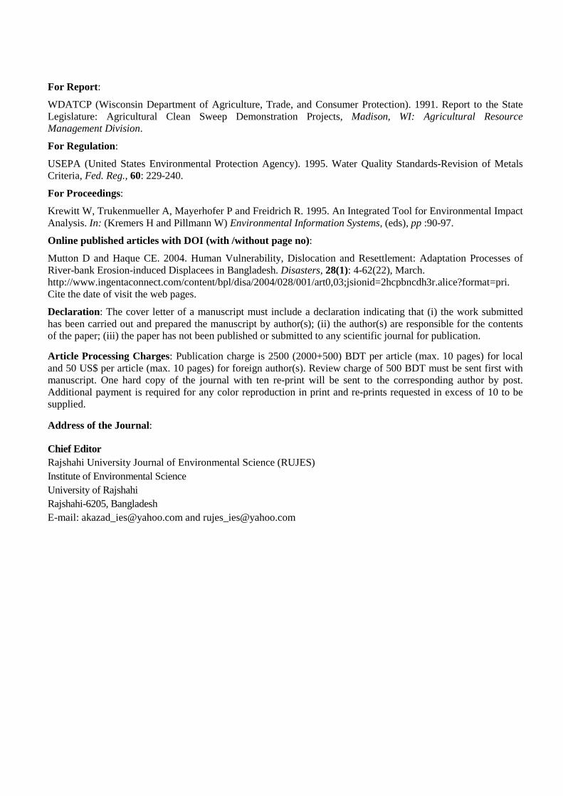
CONTENTS
Articles Pages Organic Geochemical Investigation of Permian Gondwana Shales from Drillhole GDH-46, Khalaspir Basin, Bangladesh: Implications for Source and Depositional Environment
Quazi Hasna Hossain, H. M. Zakir Hossain, Shigeyuki Suzuki, Yoshikazu Sampei, Toshiro Yamanaka, Yuji Onishi and Md. and Sultan-Ul-Islam
01-10
Reduction of Vegetation Cover in Rajshahi City Corporation of Bangladesh Abdulla-Al Kafy, Golam Sabbir Sattar, and Syed Mahmud-ul-islam
11-24
Efficacy of Some Botanical Extracts against Late Blight of Potato in Experimental Field Shafiqul Islam, Md. Abul Kalam Azad and Md. Rashidul Islam
25-32
Germination and Seedling Growth Performance of Benincasa hispida (Thunb.) Cogn. in Arsenic Solution Cultures under Phosphorus Amendment Bayezid Mahmud Khan, Afroza Hasan Afrin, Mohammad Mosharraf Hossain and Ismail Md. Mofizur Rahman
33-42
Assessing the Potentiality of Five Medicinal Plant Extracts to Control the Thrips (Scirtothrips bispinosus) of Tea Garden Md. Abul Kalam Azad, Iftekhar Ahmad and Moinuddin Ahmed
43-50
Some Biological Parameters of Asian Stinging Catfish, Heteropneustes fossilis (Bloch, 1794) (Teleostei: Siluriformes) in the Padma River Most. Farida Parvin, Akhery Nima, Farzana Akter Rima and Md. Yeamin Hossain
51-58
Evaluation of Groundwater Quality in Bagerhat District, Bangladesh Md Iqbal Hossain, A.H.M. Selim Reza, S. M. Shafiuzzaman and Md. Sultan-Ul-Islam
59-70
Usages and Impacts of Quinalphos in Commercial Aquaculture in Rajshahi, Bangladesh Md. Mokhlesur Rahman and M. Nazrul Islam
71-78
Adaptation Strategies of GOs and NGOs for Flood Management in the Teesta Floodplain Area in Rangpur District of Bangladesh Mst. Shifat Rumana
79-92
Low Back Pain among Farmers during Harvesting: A Systematic Review Md Abu Talha, Md. Redwanur Rahman, Zakiya Yasmin, Md. Nurul Islam and Md. Ruhul Amin
93-100
Effect of Weather Conditions on Stroke: A Review Md. Ruhul Amin, Md. Redwanur Rahman, Md. Moniruzzaman Sarker, Md. Nurul Islam and Tanvir Haider
101-110
Suitability and Economic Profitability of Land Conversion for Mango Orchard in Charghat Upazila, Rajshahi Kazi Thahamina Akther, S.M. Shafiuzzaman, Md. Sokman Ali and Md. Redwanur Rahman
111-120
Potentiation of Burmese Pink Cassia Cassia renigera Benth Extracts against Brine Shrimp Nauplii Artemia salina (L.) and Lymnaea acuminata Lamarck Meherun Nesa, Sahadat Hossain, Sadia Afrin Rimi and Nurul Islam
121-126
Vector Control Potentials of Mentha Piperita L. Nayeema Parvin, H.S. Jahidul Ferdous and Nurul Islam
127-134
Assessment of Heavy Metals in Some Fruit Samples from Local Market in Rajshahi City, Rajshahi, Bangladesh N. Mollica, M.M.A Mollah, M.R. Zaman and S. M. A. Salam
135-146
Quazi Hasna Hossain et al. / Rajshahi University Journal of Environmental Science, 8: 01-10, 2019 www.ru.ac.bd/ies
Organic Geochemical Investigation of Permian Gondwana Shales from Drillhole GDH-46, Khalaspir Basin, Bangladesh: Implications for Source and
Depositional Environment
Quazi Hasna Hossain1,2∗ , H. M. Zakir Hossain1, Shigeyuki Suzuki2, Yoshikazu Sampei3, Toshiro Yamanaka2,4, Yuji Onishi2,5 and Md. Sultan-Ul-Islam6
1Department of Petroleum and Mining Engineering, Jashore University of Science and Technology, Jashore 7408,
Bangladesh 2Department of Earth Sciences, Okayama University, 3-1-1 Tsushimanaka, Okayama 700-8530, Japan
3Department of Geoscience, Shimane University, 1060 Nishikawatsu, Matsue 690-8504, Japan 4Department of Ocean and Environmental Sciences, Tokyo University of Marine Science and Technology, 4-5-7 Konan
Minato-ku, Tokyo 108-8477, Japan 5Center for Ecological Research, Kyoto University, 2-509-3 Hirano, Otsu, Shiga 520-2113, Japan
6Department of Geology and Mining, University of Rajshahi, Rajshahi 6205, Bangladesh
Abstract Shales of fluvial deposits belonging to the Permian Gondwana Group, were collected from drillhole GDH-46 of the Khalaspir basin, northwestern Bangladesh, spanning the depth interval between 270 and 490 m from the surface. Here we present total organic carbon (TOC), total nitrogen (TN) and total sulfur (TS) contents, TOC/TN and TOC/TS ratios of 27 carbonaceous shale samples, in order to elucidate a significance of organic geochemical variations, sources and depositional environment of buried organic matter. The TOC and TN contents in the carbonaceous shale samples range from ~2 to 31 wt.% (average 7.64 wt.%) and 0.07 to 0.63 wt.% (average 0.27 wt.%), respectively. The TOC/TN ratios range between ~10 and 58 (average 26) indicate that organic matter in the studied shale samples were mostly originated from terrestrial vascular plants with minor input of algal derived organic matter. Furthermore, the strong positive correlation between TOC and TN (r = 0.76) suggests a comparable organic matter source with some exceptional data in the plot area of high TOC contents. TOC/TS ratios for the Gondwana shale samples varied between ~67 and 2400 (average 598), indicating mainly oxic conditions prevailed during preservation of organic matter in the Khalaspir basin.
Keywords: Gondwana shale; Organic matter; TOC/TN ratio; Permian; Khalaspir basin; Bangladesh.
1. Introduction
Geochemical characteristics of organic matter in carbonaceous shale and coal provide important information related to the sources of organic matter, paleodepositional environments and paleoclimate fingerprints. Total organic carbon (TOC), total nitrogen (TN), total sulfur (TS) and their ratio values of sedimentary rock, sediment, and coal are widely used to identify organic carbon and nitrogen influx to the terrestrial/oceanic basin (Singh et al., 2012; Ding et al., 2018). Additionally, organic geochemical proxies of coals, and coaly shales or carbonaceous shales have provided to use as a guide for terrestrial carbon cycle in the globe, redox potential, land plant/planktonic sources and to reconstruct depositional environment (Bechtel et al., 2007, 2018).
The Permian Gondwana sequence in the northwestern part of the Bengal Basin of Bangladesh contains abundant carbonaeous shales and coal seams (Islam et al. 1991; Norman, 1992; Uddin and Islam, 1992a; 1998; Bakr et al. 1996; Hossain et al., 2000, 2002, 2013). The Gondwana coal in northwestern Bangladesh is sub-bituminous to bituminous in nature (Wardell-Armstrong, 1991; Norman, 1992; Bakr et al., 1996). This Gondwana sequence has attracted the attention of geoscientists worldwide in different viewpoints, such as geology, lithostratigraphy and palynostratigraphy, sedimentology, geochemistry and coal-bed resource potential (Wardell-Armstrong, 1991; Islam 1993, 1994; Islam et al., 1992; Hossain et al., 2001, 2002; Islam and Hossain, 2006; Islam and Hayashi, 2008; Farhaduzzaman et al., 2012; Hossain et al., 2000, 2013, 2019, 2020; Islam et al. 2003, 2004a, b). The geochemical composition of Permian Gondwana coals (bituminous/sub-bituminous types) and shales around the globe have been investigated by numerous authors (Whiticar, 1996; de Wit et al., 2002; Sarkar et al., 2003; Bechtel et al., 2007; Singh et al., 2012; Ding et al., 2018). However, there are only limited organic geochemical ∗ Corresponding author’s e-mail: [email protected]
Quazi Hasna Hossain et al. / Rajshahi University Journal of Environmental Science, 8: 01-10, 2019 www.ru.ac.bd/ies
2
data published in nearby similar coal-bearing Gondwana basin in India (Sarkar et al., 2003; Singh et al., 2012; Ding et al., 2018), and none of these studies have been conducted in the Gondwana sediments from drillhole GDH-46, Khalaspir basin in Bangladesh. Therefore, this is the first proxy report describing TOC, TN and TS contents in carbonaceous shales of northwestern Bangladesh to recover varied paleovegetation types and redox conditions during Permian age. This paper reports elemental compositions of carbonaceous shales in drillhole GDH-46, Khalaspir basin, Bangladesh, and highlights their potential input of organic matter source, vertical variations in elemental composition and depositional environment during evolution of the Gondwana succession.
2. Geological Setting
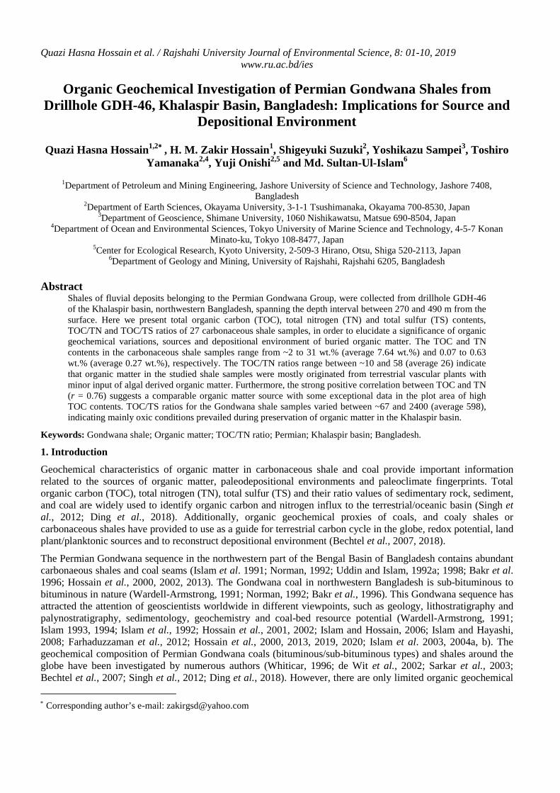
The Khalaspir basin is located in northwestern part of Bangladesh (Figure 1). This basin has an elongated fault bounded NW-SE trending composite outline with an area of approximately 25 km2, and contains probable coal researves of about 685 Mt (Islam et al., 1992; Uddin and Islam 1992b Hossain et al., 2001, 2002). Eight coal seams were identified in the basin with a combined thickness of ~50 m, and the depth range between 257 and 483 m from the surface (Islam et al. 1992; Hossain et al., 2002). This coal-bearing Gondwana sequence was accumulated during the Permian. Stratigraphic architectures of the Khalaspir basin are categorized as Gondwana Group, Surma Group, Dupi Tila Formation, Barind clay residuum, and alluvium in ascending order (Table 1). The Gondwana Group of Permian age is the oldest sedimentary succession in the Khalaspir basin. This Group composed of conglomerate, sandstone, shale and abundant coal. The sequences which are characterized by the finning upward successions of meandering river deposits are common. Feldspar is major in sandstone composition. Some sandstones and shales are calcareous due to formation of caliche. The conglomerate is predominant in the lower part of the Gondwana Group, which occurs in fluid flow or debris flow dominating braided river environment (Uddin and Islam 1992b; Hossain et al., 2002). The coarse-grained sandstone in middle and upper part of this Gondwana Group is accumulated in braided river environment. The Miocene Surma Group is unconformably overlying the Gondwana Group, composed mainly of grey to dark grey mudstone, sandstone and pebbly sandstone (Hossain et al., 2001). This Group was deposited in fluvial environment under channel-floodplain system (Islam et al., 1992; Uddin and Islam 1992b; Hossain et al., 2002). The Dupi Tila Group consists mainly of grey to yellowish grey sandstone, pebbly sandstone with uncommon mudstone (Table 1). The Pleistocene Barind Clay is unconformably underlying the recent alluvium, which is characterizing of weathering of floodplain deposits.
Figure 1. Generalized map showing location of the investigated area and major geologic features of the Bengal
Basin and adjoining areas (modified after Hossain et al., 2013, 2019).
Quazi Hasna Hossain et al. / Rajshahi University Journal of Environmental Science, 8: 01-10, 2019 www.ru.ac.bd/ies
3
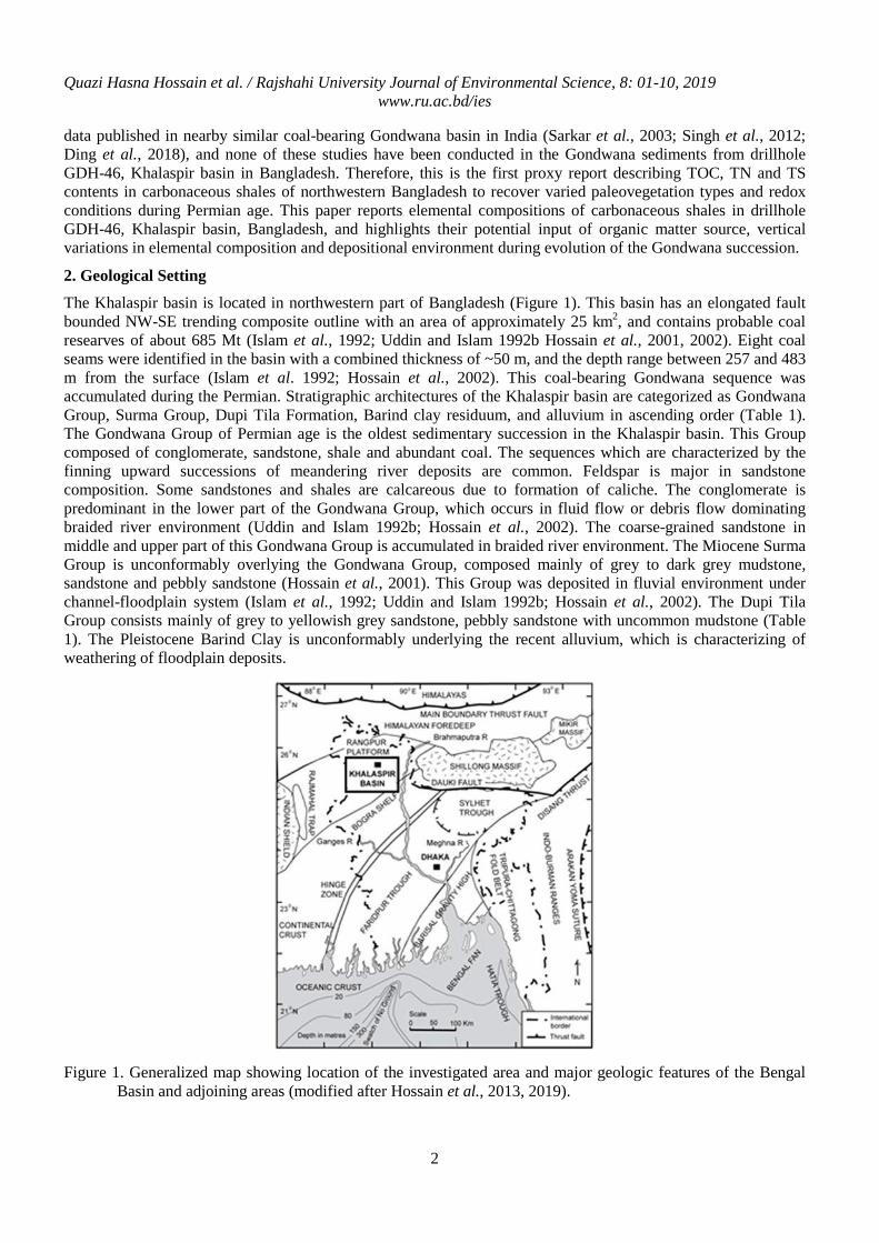
Table 1. Generalized stratigraphic succession of coal-bearing Gondwana sequence in the Khalaspir basin, northwestern Bangladesh (After Islam et al., 1992).
Age Group/Formation Lithology Max. Thickness (m)
Holocene Alluvium Grey sand and silty clay. 4.26
Pleistocene Barind Clay Yellowish grey silty clay. 6.10
Pliocene Dupi Tila Formation Grey to yellowish grey sandstone, pebbly sandstone with uncommon mudstone.
162.12
Miocene Surma Group Grey to dark grey mudstone, sandstone and pebbly sandstone.
184.14
Permian Gondwana Group Feldspathic sandstone, carbonaceous sandstone, carbonaceous shale, siltstone, mudstone, coal and conglomerate.
814.93 +
Base not seen
3. Samples and Analytical Methods
3.1. Sampling
Twenty-seven carbonaceous shale samples (ca. 100 g) were collected from the drillhole GDH-46 in the Khalaspir basin, Bangladesh. The drilled core depth was nearly 500 m, and the sampling points covered a range from 274 to 487 m within the drillhole GDH-46 (Table 2). All given samples were then taken to the organic geochemical laboratory at Shimane University and Okayama University in Japan for analysis. The cleaned carbonaceous shale samples were pulverized using hand morter and pestle subsequently stored in the laboratory.
3.2. CNS Elemental Analysis
TOC, TN and TS analyses were performed on powdered carbonaceous shale samples with Elemental Analyzer (FISSION, EA 1108) at Shimane University, Japan. TOC and TN analysis of selected 22 carbonaceous shale samples were also conducted using an elemental analyzer (Euro EA3000, EuroVecrtor, Italy) at Okayama University, Japan. The powdered carbonaceous shales (ca. 10 mg) were pre-treated with l M HCl at room temperature to remove inorganic carbonate subsequently drying at 40 °C. The TOC and TN values were reported as weight percentage (wt.%). The analytical uncertainity (coefficient of variation) of TOC and TN was about ± 0.3 wt.%.
4. Results
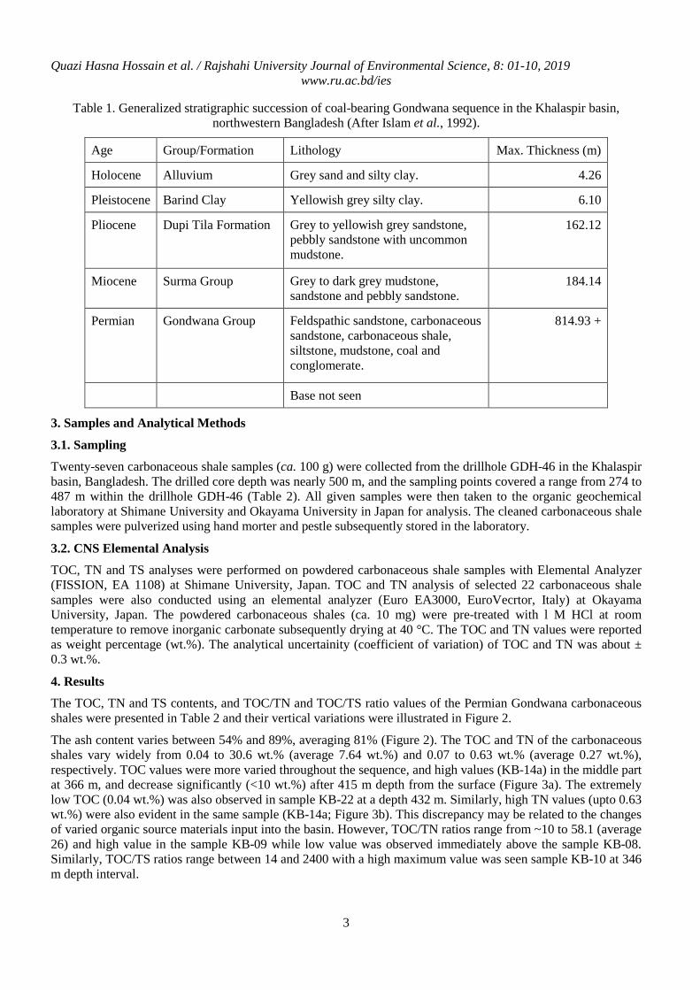
The TOC, TN and TS contents, and TOC/TN and TOC/TS ratio values of the Permian Gondwana carbonaceous shales were presented in Table 2 and their vertical variations were illustrated in Figure 2.
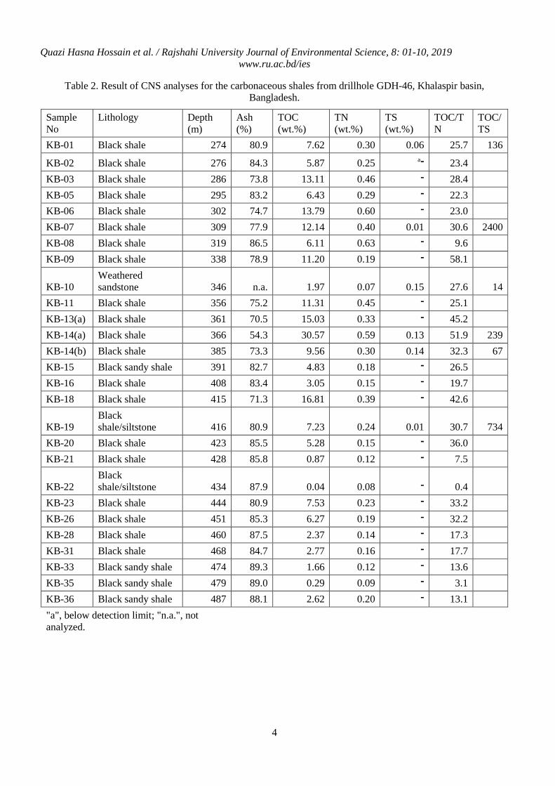
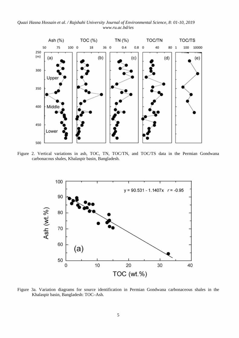
The ash content varies between 54% and 89%, averaging 81% (Figure 2). The TOC and TN of the carbonaceous shales vary widely from 0.04 to 30.6 wt.% (average 7.64 wt.%) and 0.07 to 0.63 wt.% (average 0.27 wt.%), respectively. TOC values were more varied throughout the sequence, and high values (KB-14a) in the middle part at 366 m, and decrease significantly (<10 wt.%) after 415 m depth from the surface (Figure 3a). The extremely low TOC (0.04 wt.%) was also observed in sample KB-22 at a depth 432 m. Similarly, high TN values (upto 0.63 wt.%) were also evident in the same sample (KB-14a; Figure 3b). This discrepancy may be related to the changes of varied organic source materials input into the basin. However, TOC/TN ratios range from ~10 to 58.1 (average 26) and high value in the sample KB-09 while low value was observed immediately above the sample KB-08. Similarly, TOC/TS ratios range between 14 and 2400 with a high maximum value was seen sample KB-10 at 346 m depth interval.
Quazi Hasna Hossain et al. / Rajshahi University Journal of Environmental Science, 8: 01-10, 2019 www.ru.ac.bd/ies
4
Table 2. Result of CNS analyses for the carbonaceous shales from drillhole GDH-46, Khalaspir basin, Bangladesh.
Sample No
Lithology Depth (m)
Ash (%)
TOC (wt.%)
TN (wt.%)
TS (wt.%)
TOC/TN
TOC/TS
KB-01 Black shale 274 80.9 7.62 0.30 0.06 25.7 136 KB-02 Black shale 276 84.3 5.87 0.25 ־P
a 23.4 KB-03 Black shale 286 73.8 13.11 0.46 28.4 ־ KB-05 Black shale 295 83.2 6.43 0.29 22.3 ־ KB-06 Black shale 302 74.7 13.79 0.60 23.0 ־ KB-07 Black shale 309 77.9 12.14 0.40 0.01 30.6 2400 KB-08 Black shale 319 86.5 6.11 0.63 9.6 ־ KB-09 Black shale 338 78.9 11.20 0.19 58.1 ־
KB-10 Weathered sandstone 346 n.a. 1.97 0.07 0.15 27.6 14
KB-11 Black shale 356 75.2 11.31 0.45 25.1 ־ KB-13(a) Black shale 361 70.5 15.03 0.33 45.2 ־ KB-14(a) Black shale 366 54.3 30.57 0.59 0.13 51.9 239 KB-14(b) Black shale 385 73.3 9.56 0.30 0.14 32.3 67 KB-15 Black sandy shale 391 82.7 4.83 0.18 26.5 ־ KB-16 Black shale 408 83.4 3.05 0.15 19.7 ־ KB-18 Black shale 415 71.3 16.81 0.39 42.6 ־
KB-19 Black shale/siltstone 416 80.9 7.23 0.24 0.01 30.7 734
KB-20 Black shale 423 85.5 5.28 0.15 36.0 ־ KB-21 Black shale 428 85.8 0.87 0.12 7.5 ־
KB-22 Black shale/siltstone 434 87.9 0.04 0.08 0.4 ־
KB-23 Black shale 444 80.9 7.53 0.23 33.2 ־ KB-26 Black shale 451 85.3 6.27 0.19 32.2 ־ KB-28 Black shale 460 87.5 2.37 0.14 17.3 ־ KB-31 Black shale 468 84.7 2.77 0.16 17.7 ־ KB-33 Black sandy shale 474 89.3 1.66 0.12 13.6 ־ KB-35 Black sandy shale 479 89.0 0.29 0.09 3.1 ־ KB-36 Black sandy shale 487 88.1 2.62 0.20 13.1 ־ "a", below detection limit; "n.a.", not analyzed.
Quazi Hasna Hossain et al. / Rajshahi University Journal of Environmental Science, 8: 01-10, 2019 www.ru.ac.bd/ies
5
Figure 2. Vertical variations in ash, TOC, TN, TOC/TN, and TOC/TS data in the Permian Gondwana
carbonacous shales, Khalaspir basin, Bangladesh.
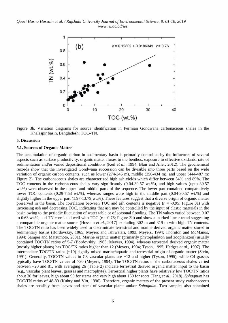
Figure 3a. Variation diagrams for source identification in Permian Gondwana carbonaceous shales in the Khalaspir basin, Bangladesh: TOC–Ash.
Quazi Hasna Hossain et al. / Rajshahi University Journal of Environmental Science, 8: 01-10, 2019 www.ru.ac.bd/ies
6
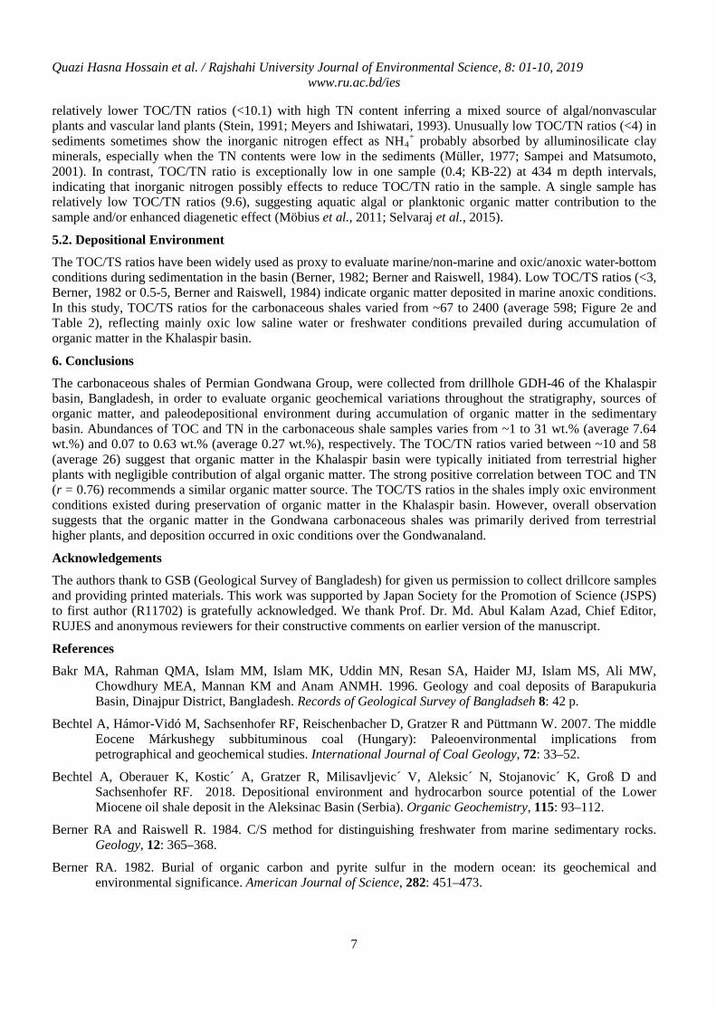
Figure 3b. Variation diagrams for source identification in Permian Gondwana carbonaceous shales in the Khalaspir basin, Bangladesh: TOC–TN.
5. Discussion
5.1. Sources of Organic Matter
The accumulation of organic carbon in sedimentary basin is primarily controlled by the influences of several aspects such as surface productivity, organic matter fluxes to the benthos, exposure to effective oxidants, rate of sedimentation and/or varied depositional conditions (Keil et al., 1994; Blair and Aller, 2012). The geochemical records show that the investigated Gondwana succession can be divisible into three parts based on the wide variation of organic carbon contents, such as lower (274-346 m), middle (356-434 m), and upper (444-487 m: Figure 2). The carbonaceous shales are characterized high ash yields which differ between 54% and 89%. The TOC contents in the carbonaceous shales vary significantly (0.04-30.57 wt.%), and high values (upto 30.57 wt.%) were observed in the upper- and middle parts of the sequence. The lower part contained comparatively lower TOC contents (0.29-7.53 wt.%), whereas ranges were high in the middle part (0.04-30.57 wt.%) and slightly higher in the upper part (1.97-13.79 wt.%). These features suggest that a diverse origin of organic matter preserved in the basin. The correlation between TOC and ash contents is negative (r = -0.95; Figure 3a) with increasing ash and decreasing TOC, indicating that ash may be controlled by the input of clastic materials in the basin owing to the periodic fluctuation of water table or of seasonal flooding. The TN values varied between 0.07 to 0.63 wt.%, and TN correlated well with TOC (r = 0.76; Figure 3b) and show a marked linear trend suggesting a comparable organic matter source (Hossain et al., 2017) excluding 302 m and 319 m with high TN contents. The TOC/TN ratio has been widely used to discriminate terrestrial and marine derived organic matter stored in sedimentary basins (Bordovskiy, 1965; Meyers and Ishiwatari, 1993; Meyers, 1994; Thornton and McManus, 1994; Sampei and Matsumoto, 2001). Marine organic matter (primarily phytoplankton and zooplankton) usually contained TOC/TN ratios of 5-7 (Bordovskiy, 1965; Meyers, 1994), whereas terrestrial derived organic matter (mostly higher plants) has TOC/TN ratios higher than 12 (Meyers, 1994; Tyson, 1995; Hedges et al., 1997). The intermediate TOC/TN ratios (~10) signify mixed marine/aquatic and terrestrial origin of organic matter (Stein, 1991). Generally, TOC/TN values in C3 vascular plants are ~12 and higher (Tyson, 1995), while C4 grasses typically have TOC/TN values of >30 (Meyers, 1994). The TOC/TN ratios in the carbonaceous shales varied between ~20 and 81, with averaging 26 (Table 2) indicate terrestrial derived organic matter input to the basin (e.g., vascular plant leaves, grasses and macrophyte). Terrestrial higher plants have relatively low TOC/TN ratios about 30 for leaves, high about 90 for stems and very high about 150 for roots (Tang et al., 2018). Sphagnum has TOC/TN ratios of 48-89 (Kuhry and Vitt, 1996). Therefore, organic matters of the present study carbonaceous shales are possibly from leaves and stems of vascular plants and/or Sphagnum. Two samples also contained
Quazi Hasna Hossain et al. / Rajshahi University Journal of Environmental Science, 8: 01-10, 2019 www.ru.ac.bd/ies
7
relatively lower TOC/TN ratios (<10.1) with high TN content inferring a mixed source of algal/nonvascular plants and vascular land plants (Stein, 1991; Meyers and Ishiwatari, 1993). Unusually low TOC/TN ratios (<4) in sediments sometimes show the inorganic nitrogen effect as NH4
+ probably absorbed by alluminosilicate clay minerals, especially when the TN contents were low in the sediments (Müller, 1977; Sampei and Matsumoto, 2001). In contrast, TOC/TN ratio is exceptionally low in one sample (0.4; KB-22) at 434 m depth intervals, indicating that inorganic nitrogen possibly effects to reduce TOC/TN ratio in the sample. A single sample has relatively low TOC/TN ratios (9.6), suggesting aquatic algal or planktonic organic matter contribution to the sample and/or enhanced diagenetic effect (Möbius et al., 2011; Selvaraj et al., 2015).
5.2. Depositional Environment
The TOC/TS ratios have been widely used as proxy to evaluate marine/non-marine and oxic/anoxic water-bottom conditions during sedimentation in the basin (Berner, 1982; Berner and Raiswell, 1984). Low TOC/TS ratios (<3, Berner, 1982 or 0.5-5, Berner and Raiswell, 1984) indicate organic matter deposited in marine anoxic conditions. In this study, TOC/TS ratios for the carbonaceous shales varied from ~67 to 2400 (average 598; Figure 2e and Table 2), reflecting mainly oxic low saline water or freshwater conditions prevailed during accumulation of organic matter in the Khalaspir basin.
6. Conclusions
The carbonaceous shales of Permian Gondwana Group, were collected from drillhole GDH-46 of the Khalaspir basin, Bangladesh, in order to evaluate organic geochemical variations throughout the stratigraphy, sources of organic matter, and paleodepositional environment during accumulation of organic matter in the sedimentary basin. Abundances of TOC and TN in the carbonaceous shale samples varies from ~1 to 31 wt.% (average 7.64 wt.%) and 0.07 to 0.63 wt.% (average 0.27 wt.%), respectively. The TOC/TN ratios varied between ~10 and 58 (average 26) suggest that organic matter in the Khalaspir basin were typically initiated from terrestrial higher plants with negligible contribution of algal organic matter. The strong positive correlation between TOC and TN (r = 0.76) recommends a similar organic matter source. The TOC/TS ratios in the shales imply oxic environment conditions existed during preservation of organic matter in the Khalaspir basin. However, overall observation suggests that the organic matter in the Gondwana carbonaceous shales was primarily derived from terrestrial higher plants, and deposition occurred in oxic conditions over the Gondwanaland.
Acknowledgements
The authors thank to GSB (Geological Survey of Bangladesh) for given us permission to collect drillcore samples and providing printed materials. This work was supported by Japan Society for the Promotion of Science (JSPS) to first author (R11702) is gratefully acknowledged. We thank Prof. Dr. Md. Abul Kalam Azad, Chief Editor, RUJES and anonymous reviewers for their constructive comments on earlier version of the manuscript.
References
Bakr MA, Rahman QMA, Islam MM, Islam MK, Uddin MN, Resan SA, Haider MJ, Islam MS, Ali MW, Chowdhury MEA, Mannan KM and Anam ANMH. 1996. Geology and coal deposits of Barapukuria Basin, Dinajpur District, Bangladesh. Records of Geological Survey of Bangladseh 8: 42 p.
Bechtel A, Hámor-Vidó M, Sachsenhofer RF, Reischenbacher D, Gratzer R and Püttmann W. 2007. The middle Eocene Márkushegy subbituminous coal (Hungary): Paleoenvironmental implications from petrographical and geochemical studies. International Journal of Coal Geology, 72: 33–52.
Bechtel A, Oberauer K, Kostic´ A, Gratzer R, Milisavljevic´ V, Aleksic´ N, Stojanovic´ K, Groß D and Sachsenhofer RF. 2018. Depositional environment and hydrocarbon source potential of the Lower Miocene oil shale deposit in the Aleksinac Basin (Serbia). Organic Geochemistry, 115: 93–112.
Berner RA and Raiswell R. 1984. C/S method for distinguishing freshwater from marine sedimentary rocks. Geology, 12: 365–368.
Berner RA. 1982. Burial of organic carbon and pyrite sulfur in the modern ocean: its geochemical and environmental significance. American Journal of Science, 282: 451–473.
Quazi Hasna Hossain et al. / Rajshahi University Journal of Environmental Science, 8: 01-10, 2019 www.ru.ac.bd/ies
8
Blair NE and Aller RC. 2012. The fate of terrestrial organic carbon in the marine environment. Annual Review of Marine Science, 4: 401–423.
Bordovskiy OK. 1965. Accumulation of organic matter in bottom sediments. Marine Geology, 3: 33–82.
de Wit MJ, Ghosh SC, Joy G, de Villiers S, Rakotosolofo N, Alexander J, Tripathi A and Looy C. 2002. Multiple organic carbon isotope reversals across the Permo-Triassic boundary of terrestrial Gondwana sequences: clues to extinction patterns and delayed ecosystem recovery. Journal of Geology, 110: 227–240.
Ding D, Liu G, Sun X and Sun R. 2018. Response of carbon isotopic compositions of Early-Middle Permian coals in North China to palaeo-climate change. Journal of Asian Earth Sciences, 151: 190–196.
Farhaduzzaman M, Abdullah WH and Islam MA. 2012. Depositional environment and hydrocarbon source potential of the Permian Gondwana coals from the Barapukuria Basin, Northwest Bangladesh. International Journal of Coal Geology, 90–91: 162–179.
Hedges JI, Keil RG and Benner R. 1997. What happens to terrestrial organic matter in the ocean? Organic Geochemistry, 27: 195–212.
Hossain HMZ, Hossain QH, Kamei A, Araoka D and Islam MS. 2020. Geochemical characteristics of Gondwana shales from the Barapukuria basin, Bangladesh: Implications for source-area weathering and provenance. Arabian Journal of Geosciences, 13(3): 111, https://doi.org/10.1007/s12517-020-5105-6.
Hossain HMZ, Islam MS, Ahmed SS and Hossain I. 2001. Petrography of Gondwana sandstones in the borehole GDH-45 of the Khalaspir Basin, Bangladesh. Acta Mineralogica Pakistanica, 12: 63–74.
Hossain HMZ, Islam MS, Ahmed SS and Hossain I. 2002. Analysis of sedimentary facies and depositional environments of the Permian Gondwana sequence in borehole GDH-45, Khalaspir Basin, Bangladesh. Geosciences Journal, 6: 227–236.
Hossain HMZ, Kawahata H, Roser BP, Sampei Y, Manaka T and Otani S. 2017. Geochemical characteristics of modern river sediments in Myanmar and Thailand: implications for provenance and weathering. Chemie der Erde, 77: 443–458.
Hossain HMZ, Sampei Y, Hossain QH, Roser BP and Islam MS. 2013. Characterization of alkyl phenanthrene distributions in Permian Gondwana coals and coaly shales from the Barapukuria basin, NW Bangladesh. Researches in Organic Geochemistry, 29: 17−28.
Hossain HMZ, Sampei Y, Hossain QH, Yamanaka T, Roser BP and Islam MS. 2019. Origin of organic matter and hydrocarbon potential of Permian Gondwana coaly shales intercalated in coals/sands of the Barapukuria basin, Bangladesh. International Journal of Coal Geology, 212: 103201, doi.org/10.1016/j.coal.2019.05.008.
Hossain I, Ahmed SS and Islam MS. 2000. Provenance of Gondwana sandstones in the borehole GDH-40, Barapukuria basin, Dinajpur, Bangladesh. Bangladesh Journal of Geology, 19:35-44.
Islam MN, Uddin MN, Resan SA, Islam MS and Ali MW. 1992. Geology of the Khalaspir coal basin, Pirganj, Rangpur, Bangladesh. Records of Geological Survey of Bangladesh, 6(5): 809 p.
Islam MR and Hayashi D. 2008. Geology and coal bed methane resource potential of the Gondwana Barapukuria Coal Basin, Dinajpur, Bangladesh. International Journal of Coal Geology, 75: 127–143.
Islam MS and Hossain I. 2006. Lithofacies and embedded Markov chain analyses of Gondwana sequence in boreholes GDH-40 and 43, Barapukuria coalfield, Bangladesh. Bangladesh Journal of Geology, 25: 64–84.
Islam MS, Chowdhury KR and Ishiga H. 2004. Geochemistry of the Gondwana sedimentary rocks from the Barapukuria basin, Bangladesh. Bangladesh Geoscience Journal, 10:83-102.
Islam MS, D’Rozario A, Chowdhury KR and Banerjee M. 2003. Palynostratigraphy of the Gondwana Sequence in the Barapukuria coal basin, Bangladesh. Bangladesh Geoscience Journal, 9:1-29.
Quazi Hasna Hossain et al. / Rajshahi University Journal of Environmental Science, 8: 01-10, 2019 www.ru.ac.bd/ies
9
Islam MS, D’Rozario A, Chowdhury KR and Banerjee M. 2004. Palynoassemblages and Paleovegetation of the Gondwana rocks in the Barapukuria coal basin, Bangladesh, Bangladesh Journal of Geology, 23:13-31.
Islam MS. 1993. Anatomy and depositional environment of the abnormally thick coal seam VI in the Barapukuria basin, Dinajpur, Bangladesh. Bangladesh Journal of Geology, 12:27-38.
Islam MS. 1994. Gondwana coal resources of Bangladesh and their characteristics. Proceedings of Second SEGMITE International Conference, Pakistan, 2:85-90.
Islam MS. 1998. Origin of thick coal seam in the Gondwana Sequence of the Jamalganj basin, Bangladesh. Journal of Nepal Geological Society, 18:289-298.
Keil RG, Montluçon DB, Prahl FG and Hedges JI. 1994. Sorptive preservation of labile organic matter in marine sediments. Nature, 370: 549–552.
Kuhry P and Vitt DH. 1996. Fossil carbon/nitrogen ratios as a measure of peat decomposition. Ecology, 77(1): 271–275.
Meyers PA and Ishiwatari R. 1993. Lacustrine organic geochemistry – an overview of indicators of organic matter sources and diagenesis in lake sediments. Organic Geochemistry, 20: 867–900.
Meyers PA. 1994. Preservation of elemental and isotopic source identification of sedimentary organic matter. Chemical Geology, 114: 289–302.
Möbius J, Gaye B, Lahajnar N, Bahlmann E and Emeis K-C. 2011. Influence of diagenesis on sedimentary δ15N in the Arabian Sea over the last 130 kyr. Marine Geology, 284: 127–138.
Müller PJ. 1977. C/N ratios in Pacific deep-sea sediments: effect of inorganic ammonium and organic nitrogen compounds sorbed by clays. Geochimica et Cosmochimica Acta, 41: 765–776.
Norman PS. 1992. Evaluation of the Barapukuria coal deposit NW Bangladesh. In: (Annels AE; ed): Case Histories and Methods in Mineral Resource Evaluation. Geological Society Special Publication, 63: 107–120.
Sampei Y and Matsumoto E. 2001. C/N ratios in a sediment core from Nakaumi Lagoon, southwest Japan–usefulness as an organic source indicator. Geochemical Journal, 35: 189–205.
Sarkar A, Yoshioka H, Ebihara M and Naraoka H. 2003. Geochemical and organic carbon isotope studies across the continental Permo-Triassic boundary of Raniganj Basin, eastern India. Palaeogeography, Palaeoclimatology, Palaeoecology, 191: 1–14.
Selvaraj K, Lee TY, Yang JYT, Canuel EA, Huang JC, Dai M, Liu JT and Kao SJ. 2015. Stable isotopic and biomarker evidence of terrigenous organic matter export to the deep sea during tropical storms. Marine Geology, 364: 32–42.
Singh PK, Singh MP, Prachiti PK, Kalpana MS, Manikyamba C, Lakshminarayana G, Singh AK and Naik AS. 2012. Petrographic characteristics and carbon isotopic composition of Permian coal: implications on depositional environment of Sattupalli coalfield, Godavari Valley, India. International Journal of Coal Geology, 90: 34–42.
Stein R. 1991. Accumulation of organic carbon in marine sediments. Results from the Deep Sea Drilling Project/Ocean Drilling Program. Lecture Notes in Earth Sciences, 34: Springer-Verlag, Berlin (pp. 217).
Tang Z, Xu W, Zhou G, Bai Y, Li J, Tang X, Chen D, Liu Q, Ma W, Xiong G, He H, He N, Guo Y, Guo Q, Zhu J, Han W, Hu H, Fang J and Xie Z. 2018. Patterns of plant carbon, nitrogen, and phosphorus concentration in relation to productivity in China’s terrestrial ecosystems. Proceedings of the National Academy of Sciences, 115: 4033–4038.
Thornton SF and McManus J. 1994. Application of organic carbon and nitrogen stable isotope and C/N ratios as source indicators of organic matter provenace in estuarine systems: evidence from the Tay Estuary, Scotland. Estuarine Coastal and Shelf Science, 38: 219–233.
Quazi Hasna Hossain et al. / Rajshahi University Journal of Environmental Science, 8: 01-10, 2019 www.ru.ac.bd/ies
10
Tyson RV. 1995. Sedimentary Organic Matter: Organic Facies and Palynofacies. Chapman and Hall, London.
Uddin N and Islam MS. 1992a. Gondwana basins and their coal resources in Bangladesh. Proceedings of the First South Asian Geological Congress, (GEOSAS-1), Pakistan :224-230.
Uddin N and Islam MS. 1992b. Depositional environment of the Gondwana rocks in the Khalaspir basin, Rangpur, Bangladesh, Bangladesh Journal of Geology, 11:31-44.
Wardell-Armstrong Ltd. 1991. Techno-economic feasibility study, Barapukuria coal project, Dinajpur, Bangladesh, 12 volumes. Report submitted to Ministry of Energy and Mineral Resources, Government of People’s Republic of Bangladesh (unpublished).
Whiticar MJ. 1996. Stable isotope geochemistry of coals, humic kerogens and related natural gases. International Journal of Coal Geology, 32: 191–215.
Golam Sabbir Sattar et al. / Rajshahi University Journal of Environmental Science, 8: 11-24, 2019 www.ru.ac.bd/ies
Reduction of Vegetation Cover in Rajshahi City Corporation of Bangladesh
Abdulla-Al Kafy1, Golam Sabbir Sattar2∗ and Syed Mahmud-ul-islam3
1ICLEI South Asia, Rajshahi City Corporation, Rajshahi- 6203 2Institute of Environmental Science, University of Rajshahi, Rajshahi – 6205
3Rajshahi City Corporation, Rajshahi- 6203
Abstract Multi-temporal Landsat TM/OLI satellite images have been used for the years 2000, 2010 and 2020, to classify Land Use/Land Cover (LULC) classes, a transformation between vegetation cover (VC) to an urban area (UA), directional distribution of Urban area (UA) and Vegetation Cover (VC), and variation of Land Surface Temperature (LST) in the study area. The supervised maximum likelihood classification algorithm has been used to classify the LULC maps. All the classified LULC maps demonstrated an overall accuracy of more than 85%. The spectral radiance model has been used to extract LST information from satellite images. The LULC estimation analysis suggested a significant net increase in UA areas (+15.55%) and a reduction in VC (-19.42%) from the year 2000 to 2020 respectively. The maximum temperature of the city increased to 37.75 0C in 2020 from 27.76 0C in 2000. The assessed LST showed that lower recorded temperature zones in 2000 converted into a higher temperature zone in 2020. The mean LST distribution shows growing trends and increases in UA, and reduction in VC converted the study region from a moderate temperature zone to the high-temperature zone. The study clearly show that a rise in the non-evaporated surfaces, i.e., UA and a reduction in the green cover has significantly increased the LST effect in the study area.
Keywords: Vegetation Cover; Land Surface Temperature; Remote Sensing; Rajshahi City Corporation
1. Introduction
The need for natural resources is increasing day by day with the rapid population growth in an urban area. It seems that this situation puts increasing pressure on the natural habitat (FAO, 1997). In this regard, Land Use/Land Cover (LULC) changes should be considered as the most basic information in land management (Varun et al., 2016). One of the most critical indicators of urbanization is the increase of land surface temperature (LST) with the anthropogenic heat effect and the formation of urban heat island (UHI) (Kumar et al., 2012). Metropolitan cities are warmer compared to surrounding rural areas (Huidong et al., 2018). The main reason for the formation of urban heat is warming the land surface with the effect material involving the heat due to urban development (Kaya et al, 2012) and removing vegetation covers.
The rapid unplanned transformation of vegetation cover (VC) to an urban area (UA) dramatically affects the ecosystem and biodiversity functions. LULC and LST play a crucial role in modeling the Earth's surface hydrological, ecological, agricultural, and climate processes (Meyer and Turner, 1992; Lo and Quattrochi, 2003; Kafy et al., 2020). LULC changes accelerated by rapid urbanization and created significant effects on LST (Rahman et al., 2017a; Niyogi, 2019). LST's dynamic increment creates an Urban Heat Island (UHI) effect (Ningrum, 2018; Kafy et al., 2019b). Anthropogenic heat emission increases the land's surface temperature due to its high energy consumption and subsequent decreases in vegetation and water-permeable surfaces, thereby decreasing surface temperature through evapotranspiration (Lo and Quattrochi, 2003; Chen et al., 2006). Thermal Remote Sensing (RS) data can be used to extract the spatially distributed LSTs in clear-sky conditions by calculating the upward longwave radiation from the surface area (Hart and Sailor, 2009; Bharath et al., 2013). The thermal signal acquired by RS sensor at the top of the atmosphere (TOA) is influenced by temperature and land surface emissivity parameters (Bokaie et al., 2016).
In addition to the provision for radiant surface temperature measurements, remote sensor instruments are also used to measure energy reflectance in the red and near-infrared portions of the electromagnetic spectrum, which can be used to quantify changes in vegetation conditions (Anbazhagan and Paramasivam, 2016). The lower LSTs are usually found for dense vegetative areas, but they can differ in times, locations, and vegetation distribution
∗ Corresponding author’s e-mail: [email protected]
Golam Sabbir Sattar et al. / Rajshahi University Journal of Environmental Science, 8: 11-24, 2019 www.ru.ac.bd/ies
12
types. Weng et al. (2004) found a slightly stronger negative correlation of the vegetation fraction to LST. Yue et al. (2007) have indicated a significant difference in the mean LST and normalized differential vegetation index (NDVI) values associated with different land uses. Joshi and Bhatt (2012) reported the temperature in areas with vegetation and water sources is lower than in built-up areas. Sun and Kafatos (2007) found that the correlation of LST and NDVI in the winter is positive and in warm seasons is negative.
The victims of climate change are developing and underdeveloped countries (IPCC, 2014). As a developing country, Bangladesh is one of the world's most vulnerable to climate change. The northwestern region of Bangladesh showed a signature of climate change (World Bank, 2016). LSTs are gradually increasing in this region, influenced by urbanization, global warming, and climate change (IPCC, 2014; Hossain et al., 2020). Several research studies have been conducted concerning the climate change scenarios based on the temperature, but the influence of vegetation dynamics on LST studies are limited. Kafy et al (2020a) reported an increase in the mean LST over the past two decades (1999-2009) by 9.830C and 130C in the city and district of Rajshahi respectively. Ahmed and Ahmed, 2012 have been reported an increase in temperature in Bangladesh about 0.50C. Rahman and Lateh (2017) found that during the June-August period, the temperature generally increased. The average maximum and minimum temperatures showed an increasing trend, respectively, of 50C and 30C. They also opined for the December-February period, the average maximum and minimum temperatures showed a decreasing and increasing trend of 0.1 0C and 1.60C respectively.
Geographic Information System (GIS) and RS techniques used as one of the most effective approaches in identification of the dynamics of VC losses and its impacts on LST in any area (Gallo and Tarpley, 1996; Balzter, 2000; Amiri et al., 2009; Anbazhagan and Paramasivam, 2016). VC loss's impacts on surface temperature can be easily estimated using classification techniques and spatial analysis toolsets,. The study aims to identify the VC losses using a Supervised Classification Technique (SCT) and evaluate their impacts on LST retrieved from Landsat 5TM and Landsat 8 OLI Images in Rajshahi City Corporation (RCC). It is anticipated that the study will help urban planners and policymakers to identify and take effective measures in mitigating the LST effects by increasing the VC in the study area.
2. Materials and Method
2.1. Study Area
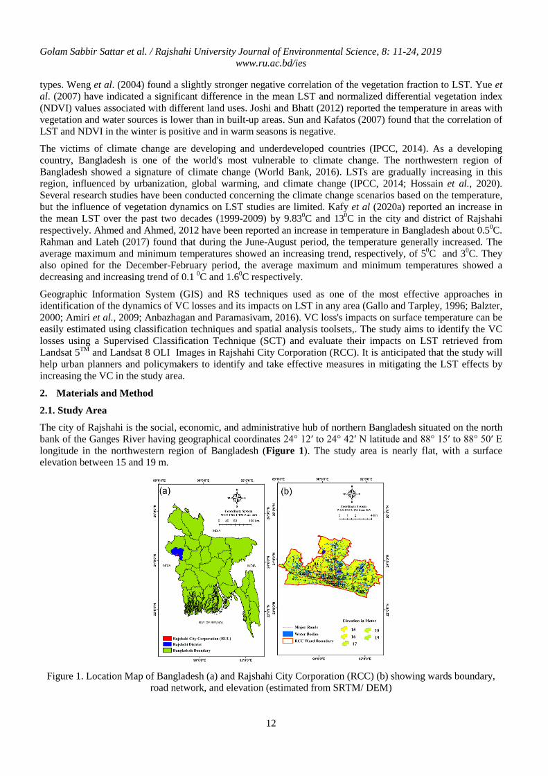
The city of Rajshahi is the social, economic, and administrative hub of northern Bangladesh situated on the north bank of the Ganges River having geographical coordinates 24° 12′ to 24° 42′ N latitude and 88° 15′ to 88° 50′ E longitude in the northwestern region of Bangladesh (Figure 1). The study area is nearly flat, with a surface elevation between 15 and 19 m.
Figure 1. Location Map of Bangladesh (a) and Rajshahi City Corporation (RCC) (b) showing wards boundary,
road network, and elevation (estimated from SRTM/ DEM)
Golam Sabbir Sattar et al. / Rajshahi University Journal of Environmental Science, 8: 11-24, 2019 www.ru.ac.bd/ies
13
The dry-wet tropical monsoonal prevails in RCC with a maximum temperature varies from 30-35 0C and having an annual average rainfall of 1448 mm (Ferdous and Baten, 2011; Kafy et al., 2020a). Since the last few decades, the city is facing rapid urbanization. Along with rapid urbanization and regional climate change phenomenon has drastically altered the duration and behavior of winter and summer seasons. This has detrimental effects on the cities climate, livelihood and green cover development (Kafy et al., 2020b). Land-use history in this area shows that over 19% of the green cover area has been lost. An increment in maximum LST was about 90C in the last 20 years due to rapid urbanization (RDA, 2003, 2008; Kafy et al., 2019c; Kafy et al., 2020b).
2.2. Data
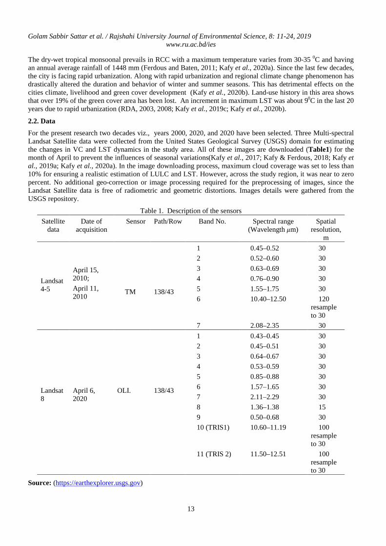
For the present research two decades viz., years 2000, 2020, and 2020 have been selected. Three Multi-spectral Landsat Satellite data were collected from the United States Geological Survey (USGS) domain for estimating the changes in VC and LST dynamics in the study area. All of these images are downloaded (Table1) for the month of April to prevent the influences of seasonal variations(Kafy et al., 2017; Kafy & Ferdous, 2018; Kafy et al., 2019a; Kafy et al., 2020a). In the image downloading process, maximum cloud coverage was set to less than 10% for ensuring a realistic estimation of LULC and LST. However, across the study region, it was near to zero percent. No additional geo-correction or image processing required for the preprocessing of images, since the Landsat Satellite data is free of radiometric and geometric distortions. Images details were gathered from the USGS repository.
Table 1. Description of the sensors Satellite
data Date of
acquisition Sensor Path/Row Band No. Spectral range
(Wavelength 𝜇m) Spatial
resolution, m
Landsat 4-5
April 15, 2010; April 11, 2010
TM
138/43
1 0.45–0.52 30 2 0.52–0.60 30 3 0.63–0.69 30 4 0.76–0.90 30 5 1.55–1.75 30 6 10.40–12.50 120
resample to 30
7 2.08–2.35 30 Landsat 8
April 6, 2020
OLI.
138/43
1 0.43–0.45 30 2 0.45–0.51 30 3 0.64–0.67 30 4 0.53–0.59 30 5 0.85–0.88 30 6 1.57–1.65 30 7 2.11–2.29 30 8 1.36–1.38 15 9 0.50–0.68 30 10 (TRIS1) 10.60–11.19 100
resample to 30
11 (TRIS 2) 11.50–12.51 100 resample to 30
Source: (https://earthexplorer.usgs.gov)
Golam Sabbir Sattar et al. / Rajshahi University Journal of Environmental Science, 8: 11-24, 2019 www.ru.ac.bd/ies
14
2.3. Landcover Classification
The satellite images obtained from Landsat sensors were enhanced in Erdas Imagine V.15 software by 3*3 majority filtering technique for better visibility (Kafy et al., 2020b; Kafy et al., 2020a). True Color Composite (TCC.) was generated using the correct band combinations for all images to choose training samples of various LULC classes (Trolle et al., 2019; Kafy et al., 2020a). The collected Landsat images were classified into four LULC categories Urban area, Vegetation cover, Water bodies, and Bare land for the years of 2000, 2010, and 2020 (Table 2). Maximum Likelihood Supervised Classification (MLSC) technique used to estimate the LULC classification. In the process of creating LULC maps, about 25 training samples were taken for each LULC class.
Accuracy of land cover maps is measured from available field data and Google Earth images through 150 ground truth points. Kappa statistics and Confusion Matrix are considered one of the best indicators for image classification accuracy were used in the study for accuracy assessment of the classified LULC maps (Story and Congalton, 1986; Foody, 2002; Congalton and Green, 2008; Pontius Jr and Millones, 2011).
Table 2. Descriptions of LULC classes
LULC Classes Description Urban area Residential, commercial and industrial services, transportation network.
Vegetation cover Trees, grassland, cropland, and fallow land. Water Bodies River, wetlands, lakes, ponds, and reservoirs.
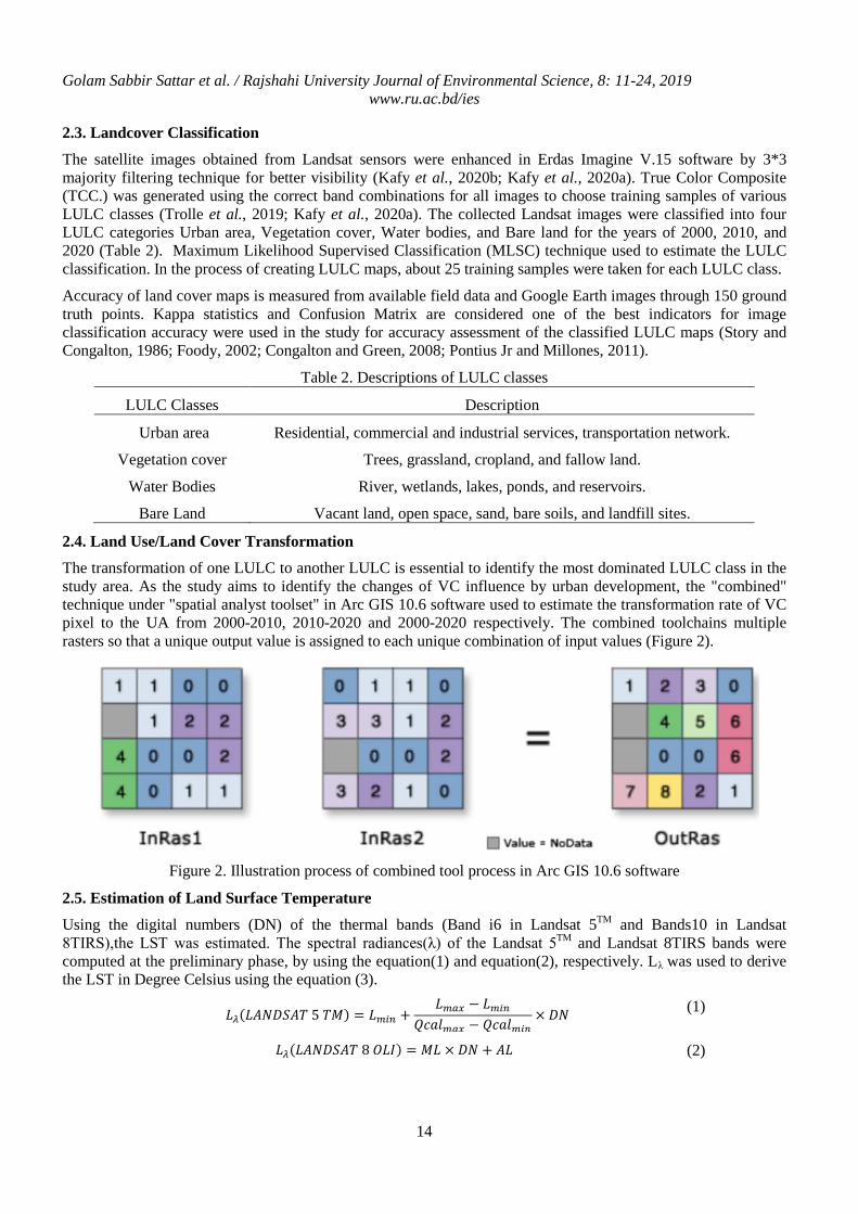
Bare Land Vacant land, open space, sand, bare soils, and landfill sites. 2.4. Land Use/Land Cover Transformation
The transformation of one LULC to another LULC is essential to identify the most dominated LULC class in the study area. As the study aims to identify the changes of VC influence by urban development, the "combined" technique under "spatial analyst toolset" in Arc GIS 10.6 software used to estimate the transformation rate of VC pixel to the UA from 2000-2010, 2010-2020 and 2000-2020 respectively. The combined toolchains multiple rasters so that a unique output value is assigned to each unique combination of input values (Figure 2).
Figure 2. Illustration process of combined tool process in Arc GIS 10.6 software
2.5. Estimation of Land Surface Temperature
Using the digital numbers (DN) of the thermal bands (Band i6 in Landsat 5TM and Bands10 in Landsat 8TIRS),the LST was estimated. The spectral radiances(λ) of the Landsat 5TM and Landsat 8TIRS bands were computed at the preliminary phase, by using the equation(1) and equation(2), respectively. Lλ was used to derive the LST in Degree Celsius using the equation (3).
𝐿𝜆(𝐿𝐴𝑁𝐷𝑆𝐴𝑇 5 𝑇𝑀) = 𝐿𝑚𝑖𝑛 +𝐿𝑚𝑎𝑥 − 𝐿𝑚𝑖𝑛
𝑄𝑐𝑎𝑙𝑚𝑎𝑥 − 𝑄𝑐𝑎𝑙𝑚𝑖𝑛× 𝐷𝑁 (1)
𝐿𝜆(𝐿𝐴𝑁𝐷𝑆𝐴𝑇 8 𝑂𝐿𝐼) = 𝑀𝐿 × 𝐷𝑁 + 𝐴𝐿 (2)
Golam Sabbir Sattar et al. / Rajshahi University Journal of Environmental Science, 8: 11-24, 2019 www.ru.ac.bd/ies
15
𝐿𝑆𝑇 =𝑇𝐵
1 + �𝜆 × 𝑇𝐵𝜌� ∗ ln (𝜀)
− 273.15 (3)
Where, ML (0.0003342) is a multiplicative rescaling factor (band-specific),and AL (0.1) is an additivere scaling factor (band-specific).The values for LandsatTM, Lmax, and Lmin were collected from the satellite meta data file. The wave length of emitted radiance λ is11.5µm (Kumar et al., 2012; Rahman et al., 2017b; Aboelnour and Engel, 2018; Ullah et al., 2019; Kafy et al., 2020a).
𝜌 =ℎ × 𝑐𝜎
= 1.438 × 10− 2 mK
(4)
Where, h indicates Plank's constant which is equal to 6.626×10⁻³⁴Js, c indicates the velocity of light, which is equal to 2.998×10⁸ms-2 and 𝜎0Tis the Boltzmann constant (5.67×10⁻⁸ iWm2k-4 i=1.38×10⁻²³JK-1); ε is the land surface emissivity which ranges in between 0.97 to 0.99 (Mallick et al., 2008; Pal and Ziaul, 2017; Guha et al., 2018).
𝑇𝐵 =𝐾2
ln (𝐾1𝐿𝜆
+ 1)
(5)
Where 𝑇𝐵 is the satellite brightness temperature, and the constants K1 and K2 values for (1) Landsat-5:K1 is 607.7, and K2 is 1260.6 and (2) Landsat8:K1 is 774.9 and K2 is 321.07, respectively (Anbazhagan and Paramasivam, 2016; Ullah et al., 2019; Kafy et al., 2020a; Roy et al., 2020).
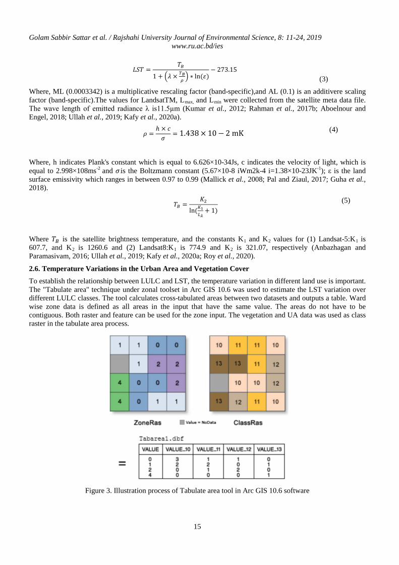
2.6. Temperature Variations in the Urban Area and Vegetation Cover
To establish the relationship between LULC and LST, the temperature variation in different land use is important. The "Tabulate area" technique under zonal toolset in Arc GIS 10.6 was used to estimate the LST variation over different LULC classes. The tool calculates cross-tabulated areas between two datasets and outputs a table. Ward wise zone data is defined as all areas in the input that have the same value. The areas do not have to be contiguous. Both raster and feature can be used for the zone input. The vegetation and UA data was used as class raster in the tabulate area process.
Figure 3. Illustration process of Tabulate area tool in Arc GIS 10.6 software
Golam Sabbir Sattar et al. / Rajshahi University Journal of Environmental Science, 8: 11-24, 2019 www.ru.ac.bd/ies
16
3. Result and Discussion
3.1. Changes in LULC Classes
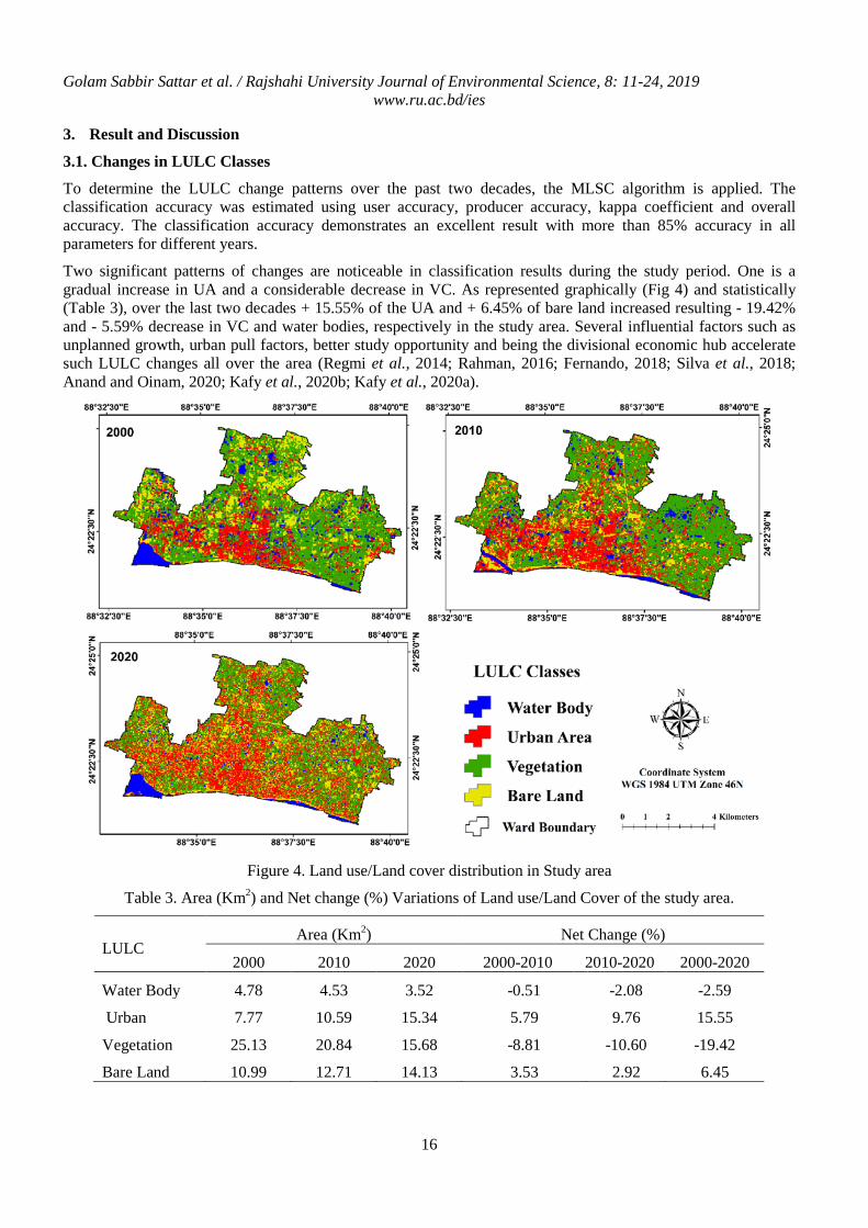
To determine the LULC change patterns over the past two decades, the MLSC algorithm is applied. The classification accuracy was estimated using user accuracy, producer accuracy, kappa coefficient and overall accuracy. The classification accuracy demonstrates an excellent result with more than 85% accuracy in all parameters for different years.
Two significant patterns of changes are noticeable in classification results during the study period. One is a gradual increase in UA and a considerable decrease in VC. As represented graphically (Fig 4) and statistically (Table 3), over the last two decades + 15.55% of the UA and + 6.45% of bare land increased resulting - 19.42% and - 5.59% decrease in VC and water bodies, respectively in the study area. Several influential factors such as unplanned growth, urban pull factors, better study opportunity and being the divisional economic hub accelerate such LULC changes all over the area (Regmi et al., 2014; Rahman, 2016; Fernando, 2018; Silva et al., 2018; Anand and Oinam, 2020; Kafy et al., 2020b; Kafy et al., 2020a).
Figure 4. Land use/Land cover distribution in Study area
Table 3. Area (Km2) and Net change (%) Variations of Land use/Land Cover of the study area.
LULC Area (Km2) Net Change (%)
2000 2010 2020 2000-2010 2010-2020 2000-2020 Water Body 4.78 4.53 3.52 -0.51 -2.08 -2.59 Urban 7.77 10.59 15.34 5.79 9.76 15.55 Vegetation 25.13 20.84 15.68 -8.81 -10.60 -19.42 Bare Land 10.99 12.71 14.13 3.53 2.92 6.45
Golam Sabbir Sattar et al. / Rajshahi University Journal of Environmental Science, 8: 11-24, 2019 www.ru.ac.bd/ies
17
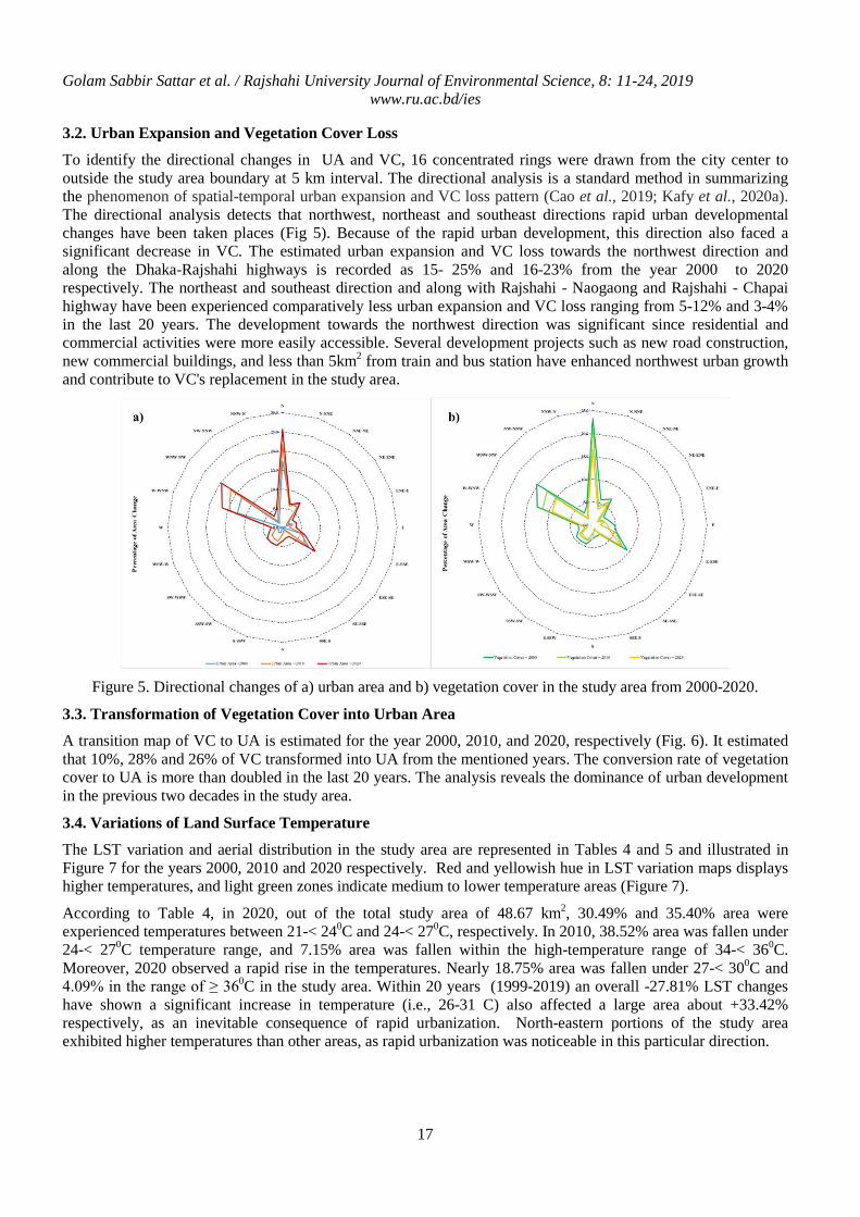
3.2. Urban Expansion and Vegetation Cover Loss
To identify the directional changes in UA and VC, 16 concentrated rings were drawn from the city center to outside the study area boundary at 5 km interval. The directional analysis is a standard method in summarizing the phenomenon of spatial-temporal urban expansion and VC loss pattern (Cao et al., 2019; Kafy et al., 2020a). The directional analysis detects that northwest, northeast and southeast directions rapid urban developmental changes have been taken places (Fig 5). Because of the rapid urban development, this direction also faced a significant decrease in VC. The estimated urban expansion and VC loss towards the northwest direction and along the Dhaka-Rajshahi highways is recorded as 15- 25% and 16-23% from the year 2000 to 2020 respectively. The northeast and southeast direction and along with Rajshahi - Naogaong and Rajshahi - Chapai highway have been experienced comparatively less urban expansion and VC loss ranging from 5-12% and 3-4% in the last 20 years. The development towards the northwest direction was significant since residential and commercial activities were more easily accessible. Several development projects such as new road construction, new commercial buildings, and less than 5km2 from train and bus station have enhanced northwest urban growth and contribute to VC's replacement in the study area.
Figure 5. Directional changes of a) urban area and b) vegetation cover in the study area from 2000-2020.
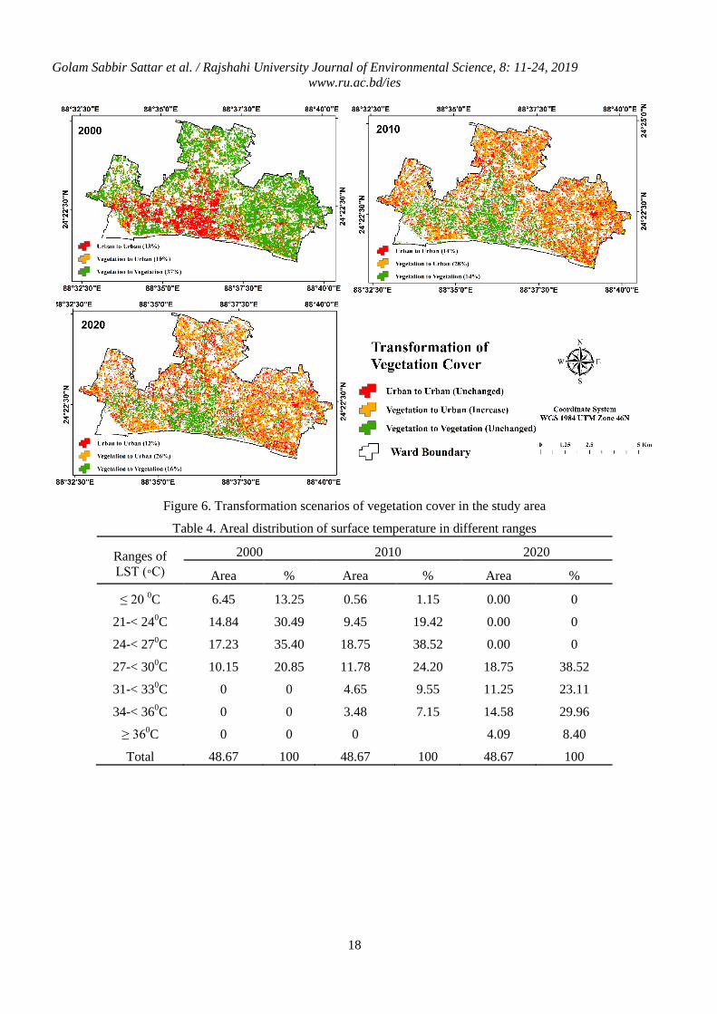
3.3. Transformation of Vegetation Cover into Urban Area
A transition map of VC to UA is estimated for the year 2000, 2010, and 2020, respectively (Fig. 6). It estimated that 10%, 28% and 26% of VC transformed into UA from the mentioned years. The conversion rate of vegetation cover to UA is more than doubled in the last 20 years. The analysis reveals the dominance of urban development in the previous two decades in the study area.
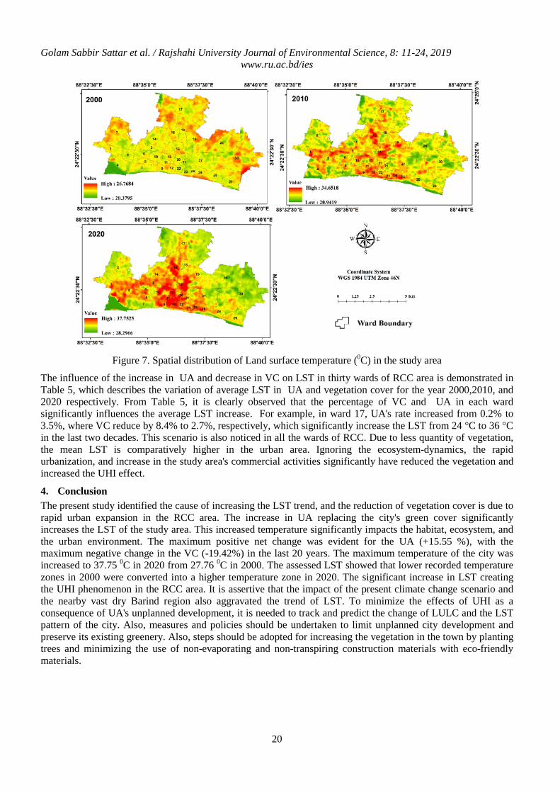
3.4. Variations of Land Surface Temperature
The LST variation and aerial distribution in the study area are represented in Tables 4 and 5 and illustrated in Figure 7 for the years 2000, 2010 and 2020 respectively. Red and yellowish hue in LST variation maps displays higher temperatures, and light green zones indicate medium to lower temperature areas (Figure 7).
According to Table 4, in 2020, out of the total study area of 48.67 km2, 30.49% and 35.40% area were experienced temperatures between 21-< 240C and 24-< 270C, respectively. In 2010, 38.52% area was fallen under 24-< 270C temperature range, and 7.15% area was fallen within the high-temperature range of 34-< 360C. Moreover, 2020 observed a rapid rise in the temperatures. Nearly 18.75% area was fallen under 27-< 300C and 4.09% in the range of ≥ 360C in the study area. Within 20 years (1999-2019) an overall -27.81% LST changes have shown a significant increase in temperature (i.e., 26-31 C) also affected a large area about +33.42% respectively, as an inevitable consequence of rapid urbanization. North-eastern portions of the study area exhibited higher temperatures than other areas, as rapid urbanization was noticeable in this particular direction.
Golam Sabbir Sattar et al. / Rajshahi University Journal of Environmental Science, 8: 11-24, 2019 www.ru.ac.bd/ies
18
Figure 6. Transformation scenarios of vegetation cover in the study area
Table 4. Areal distribution of surface temperature in different ranges
Ranges of LST (◦C)
2000 2010 2020 Area % Area % Area %
≤ 20 0C 6.45 13.25 0.56 1.15 0.00 0 21-< 240C 14.84 30.49 9.45 19.42 0.00 0 24-< 270C 17.23 35.40 18.75 38.52 0.00 0 27-< 300C 10.15 20.85 11.78 24.20 18.75 38.52 31-< 330C 0 0 4.65 9.55 11.25 23.11 34-< 360C 0 0 3.48 7.15 14.58 29.96
≥ 360C 0 0 0
4.09 8.40 Total 48.67 100 48.67 100 48.67 100
Golam Sabbir Sattar et al. / Rajshahi University Journal of Environmental Science, 8: 11-24, 2019 www.ru.ac.bd/ies
19
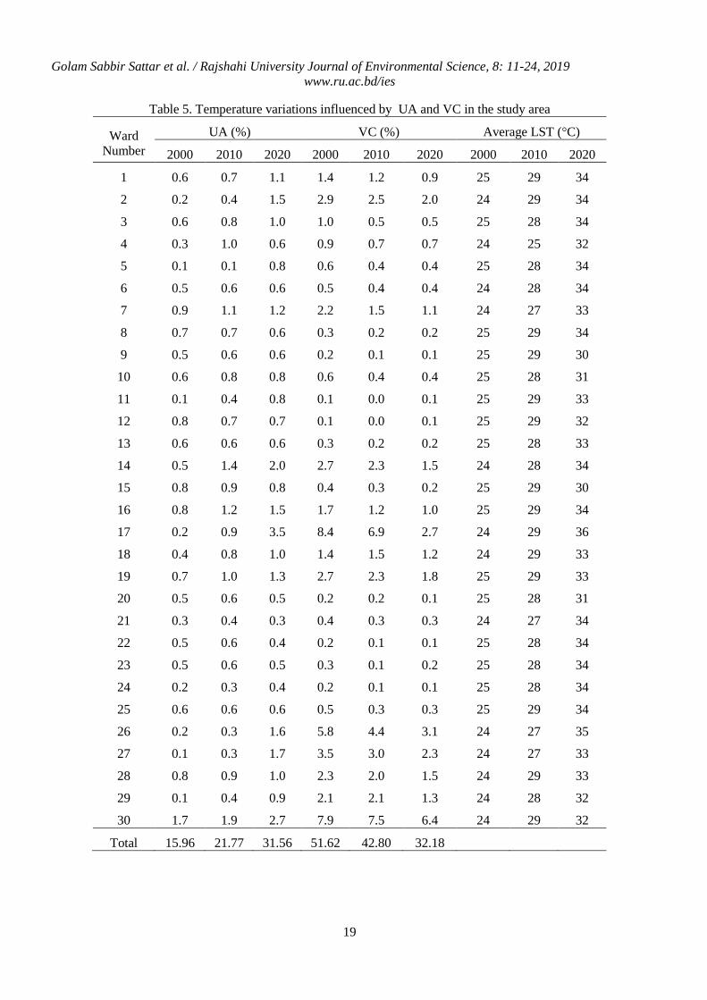
Table 5. Temperature variations influenced by UA and VC in the study area
Ward Number
UA (%) VC (%) Average LST (°C) 2000 2010 2020 2000 2010 2020 2000 2010 2020
1 0.6 0.7 1.1 1.4 1.2 0.9 25 29 34 2 0.2 0.4 1.5 2.9 2.5 2.0 24 29 34 3 0.6 0.8 1.0 1.0 0.5 0.5 25 28 34 4 0.3 1.0 0.6 0.9 0.7 0.7 24 25 32 5 0.1 0.1 0.8 0.6 0.4 0.4 25 28 34 6 0.5 0.6 0.6 0.5 0.4 0.4 24 28 34 7 0.9 1.1 1.2 2.2 1.5 1.1 24 27 33 8 0.7 0.7 0.6 0.3 0.2 0.2 25 29 34 9 0.5 0.6 0.6 0.2 0.1 0.1 25 29 30
10 0.6 0.8 0.8 0.6 0.4 0.4 25 28 31 11 0.1 0.4 0.8 0.1 0.0 0.1 25 29 33 12 0.8 0.7 0.7 0.1 0.0 0.1 25 29 32 13 0.6 0.6 0.6 0.3 0.2 0.2 25 28 33 14 0.5 1.4 2.0 2.7 2.3 1.5 24 28 34 15 0.8 0.9 0.8 0.4 0.3 0.2 25 29 30 16 0.8 1.2 1.5 1.7 1.2 1.0 25 29 34 17 0.2 0.9 3.5 8.4 6.9 2.7 24 29 36 18 0.4 0.8 1.0 1.4 1.5 1.2 24 29 33 19 0.7 1.0 1.3 2.7 2.3 1.8 25 29 33 20 0.5 0.6 0.5 0.2 0.2 0.1 25 28 31 21 0.3 0.4 0.3 0.4 0.3 0.3 24 27 34 22 0.5 0.6 0.4 0.2 0.1 0.1 25 28 34 23 0.5 0.6 0.5 0.3 0.1 0.2 25 28 34 24 0.2 0.3 0.4 0.2 0.1 0.1 25 28 34 25 0.6 0.6 0.6 0.5 0.3 0.3 25 29 34 26 0.2 0.3 1.6 5.8 4.4 3.1 24 27 35 27 0.1 0.3 1.7 3.5 3.0 2.3 24 27 33 28 0.8 0.9 1.0 2.3 2.0 1.5 24 29 33 29 0.1 0.4 0.9 2.1 2.1 1.3 24 28 32 30 1.7 1.9 2.7 7.9 7.5 6.4 24 29 32
Total 15.96 21.77 31.56 51.62 42.80 32.18
Golam Sabbir Sattar et al. / Rajshahi University Journal of Environmental Science, 8: 11-24, 2019 www.ru.ac.bd/ies
20
Figure 7. Spatial distribution of Land surface temperature (0C) in the study area
The influence of the increase in UA and decrease in VC on LST in thirty wards of RCC area is demonstrated in Table 5, which describes the variation of average LST in UA and vegetation cover for the year 2000,2010, and 2020 respectively. From Table 5, it is clearly observed that the percentage of VC and UA in each ward significantly influences the average LST increase. For example, in ward 17, UA's rate increased from 0.2% to 3.5%, where VC reduce by 8.4% to 2.7%, respectively, which significantly increase the LST from 24 °C to 36 °C in the last two decades. This scenario is also noticed in all the wards of RCC. Due to less quantity of vegetation, the mean LST is comparatively higher in the urban area. Ignoring the ecosystem-dynamics, the rapid urbanization, and increase in the study area's commercial activities significantly have reduced the vegetation and increased the UHI effect.
4. Conclusion The present study identified the cause of increasing the LST trend, and the reduction of vegetation cover is due to rapid urban expansion in the RCC area. The increase in UA replacing the city's green cover significantly increases the LST of the study area. This increased temperature significantly impacts the habitat, ecosystem, and the urban environment. The maximum positive net change was evident for the UA (+15.55 %), with the maximum negative change in the VC (-19.42%) in the last 20 years. The maximum temperature of the city was increased to 37.75 0C in 2020 from 27.76 0C in 2000. The assessed LST showed that lower recorded temperature zones in 2000 were converted into a higher temperature zone in 2020. The significant increase in LST creating the UHI phenomenon in the RCC area. It is assertive that the impact of the present climate change scenario and the nearby vast dry Barind region also aggravated the trend of LST. To minimize the effects of UHI as a consequence of UA's unplanned development, it is needed to track and predict the change of LULC and the LST pattern of the city. Also, measures and policies should be undertaken to limit unplanned city development and preserve its existing greenery. Also, steps should be adopted for increasing the vegetation in the town by planting trees and minimizing the use of non-evaporating and non-transpiring construction materials with eco-friendly materials.
Golam Sabbir Sattar et al. / Rajshahi University Journal of Environmental Science, 8: 11-24, 2019 www.ru.ac.bd/ies
21
References Aboelnour M and Engel BA. 2018. Application of Remote Sensing Techniques and Geographic Information
Systems to Analyze Land Surface Temperature in Response to Land Use/Land Cover Change in Greater Cairo Region, Egypt. Journal of Geographic Information System, 10: 57.
Ahmed B and Ahmed R. 2012. Modeling urban land cover growth dynamics using multi ‑tem poral s images: a case study of Dhaka, Bangladesh. ISPRS International Journal of Geo-Information, 1: 3-31.
Amiri R, Weng Q, Alimohammadi A and Alavipanah SK. 2009. Spatial–temporal dynamics of land surface temperature in relation to fractional vegetation cover and land use/cover in the Tabriz urban area, Iran. Remote Sensing of Environment, 113 (12): 2606-2617.
Anand V and Oinam B. 2020. Future land use land cover prediction with special emphasis on urbanization and wetlands. Remote Sensing Letters, 11: 225-234.
Anbazhagan S, and Paramasivam C. 2016. Statistical correlation between land surface temperature (LST) and vegetation index (NDVI) using multi-temporal landsat TM data. International Journal of Advanced Earth Science and Engineering, 5: 333-46.
Balzter H. 2000. Markov chain models for vegetation dynamics. Ecological modelling, 126: 139-154.
BBS, B.B.O.S. 2013. District Statistics 2011 ,Rajshahi. In: (ed. S.a.I. Division), Ministry of Planning, Government of The People's Republic of Bangladesh. 211p.
Bharath S, Rajan K and Ramachandra T. 2013. Geostatistics: An overview land surface temperature responses to land use land cover dynamics. A SciTechnol Journal, 1 (4): 158-166.
Bokaie M, Zarkesh MK, Arasteh PD and Hosseini A. 2016. Assessment of urban heat island based on the relationship between land surface temperature and land use/land cover in Tehran. Sustainable Cities and Society, 23: 94-104.
Cao H, Liu J, Chen J, Gao, J, Wang G. and Zhang W. 2019. Spatiotemporal Patterns of Urban Land Use Change in Typical Cities in the Greater Mekong Subregion (GMS). Remote Sensing, 11: 801-811.
Chen XL, Zhao HM, Li PX and Yin ZY. 2006. Remote sensing image-based analysis of the relationship between urban heat island and land use/cover changes. Remote sensing of environment, 104: 133-146.
Congalton RG and Green K. 2008. Assessing the accuracy of remotely sensed data: principles and practices. CRC press. 348p.
Ferdous M and Baten M. 2011. Climatic variables of 50 years and their trends over Rajshahi and Rangpur Division. Journal of Environmental Science and Natural Resources, 4: 147-150.
Fernando G. 2018. Identification of Urban Heat Islands & Its Relationship withVegetation Cover: A Case Study of Colombo & Gampaha Districts in Sri Lanka. Journal of Tropical Forestry and Environment, 8 (2): 82-100.
Foody GM. 2002. Status of land cover classification accuracy assessment. Remote sensing of environment, 80: 185-201.
Gallo K and Tarpley J. 1996. The comparison of vegetation index and surface temperature composites for urban heat-island analysis. International Journal of Remote Sensing, 17: 3071-3076.
Guha S, Govil H, Dey A and Gill N. 2018. Analytical study of land surface temperature with NDVI and NDBI using Landsat 8 OLI and TIRS data in Florence and Naples city, Italy. European Journal of Remote Sensing, 51: 667-678.
Golam Sabbir Sattar et al. / Rajshahi University Journal of Environmental Science, 8: 11-24, 2019 www.ru.ac.bd/ies
22
Hart MA and Sailor DJ. 2009. Quantifying the influence of land-use and surface characteristics on spatial variability in the urban heat island. Theoretical and applied climatology, 95: 397-406.
Hossain MS, Arshad M, Qian L, Kächele H, Khan I, Islam MDI and Mahboob MG. 2020. Climate change impacts on farmland value in Bangladesh. Ecological Indicators, 112: 106-118.
Huidong L, Fred M, Xuhui L, Trithankar C, Junfeg L, Martin, S and Sahar S. 2018. Interaction between urban heat islan and urban pollution island during summer in Berlin. Science of the Total Environment. 636: 818–828.
IPCC. 2014. Mitigation of climate change. Contribution of Working Group III to the Fifth Assessment Report of the Intergovernmental Panel on Climate Change, Cambridge University Press. 1454p.
Joshi JP and Bhatt B. 2012. Estimating temporal land surface temperature using remote sensing: A study of Vadodara urban area, Gujarat. International Journal of Geology, Earth and Environmental Sciences, 2: 123-130.
Kafy AA and Ferdous L. 2018. Pond Filling Locations Identification Using Landsat-8 Images In Comilla District, Bangladesh. 1st National Conference On Water Resources Engineering.
Kafy AA, Rahman MS. and Ferdous L. 2017. Exploring the Association of Land Cover Change And Landslides In The Chittagong Hill Tracts (CHT): A Remote Sensing Perspective.
Kafy AA, Islam M, Ferdous L, Khan AR and Hossain MM(a). 2019. Identifying Most Influential Land Use Parameters Contributing Reduction of Surface Water Bodies in Rajshahi City, Bangladesh: A Remote Sensing Approach. Remote Sensing of Land, 2: 87-95.
Kafy AA, Hossain M, Prince AAN, Kawshar M, Shamim MA, Das P, and Noyon MEK(b). 2019. Estimation of Land Use Change to Identify Urban Heat Island Effect on Climate change: A Remote Sensing Based Approach. International Conference on Climate Change (ICCC-2019) Dhaka, Bangladesh.
Kafy AA, Islam M, Khan A, Ferdous L and Hossain M. 2019(c). Identifying Most Influential Land Use Parameters Contributing Reduction of Surface Water Bodies in Rajshahi City, Bangladesh: A Remote Sensing Approach. Remote Sensing of Land, 2 (2): 87-95.
Kafy AA, Rahman MS, Faisal AA, Hasan MM and Islam M. 2020(a). Modelling future land use land cover changes and their impacts on land surface temperatures in Rajshahi, Bangladesh. Remote Sensing Applications: Society and Environment,
Kafy AA, Faisal AA, Sikdar S, Hasan M, Rahman M, Khan MH and Islam R. 2020(b). Impact of LULC Changes on LST in Rajshahi District of Bangladesh: A Remote Sensing Approach. Journal of Geographical Studies, 3: 11-23.
Kumar KS, Bhaskar PU and Padmakumari K. 2012 Estimation of land surface temperature to study urban heat island effect using LANDSAT ETM+ image. International journal of Engineering Science and technology, 4: 771-778.
Lo C and Quattrochi DA. 2003. Land-use and land-cover change, urban heat island phenomenon, and health implications. Photogrammetric Engineering & Remote Sensing, 69: 1053-1063.
Mallick J, Kant Y, and Bharath B. 2008. Estimation of land surface temperature over Delhi using Landsat-7 ETM+. J. Ind. Geophys. Union, 12: 131-140.
Meyer WB and Turner BL. 1992. Human population growth and global land-use/cover change. Annual review of ecology and systematics, 23: 39-61.
Golam Sabbir Sattar et al. / Rajshahi University Journal of Environmental Science, 8: 11-24, 2019 www.ru.ac.bd/ies
23
Ningrum W. 2018. Urban heat island towards urban climate. IOP Conference Series: Earth and Environmental Science.
Niyogi D. 2019. Land Surface Processes. Current Trends in the Representation of Physical Processes in Weather and Climate Models, Springer. 349-370
Pal S, and Ziaul S. 2017. Detection of land use and land cover change and land surface temperature in English Bazar urban centre. The Egyptian Journal of Remote Sensing and Space Science, 20: 125-145.
Pontius Jr RG, and Millones M. 2011. Death to Kappa: birth of quantity disagreement and allocation disagreement for accuracy assessment. International Journal of Remote Sensing, 32: 4407-4429.
Rahman M. 2016. Detection of land use/land cover changes and urban sprawl in Al-Khobar, Saudi Arabia: An analysis of multi-temporal remote sensing data. ISPRS International Journal of Geo-Information, 5 (15): 2-16.
Rahman MR. and Lateh H. 2017. Climate change in Bangladesh: a spatio-temporal analysis and simulation of recent temperature and rainfall data using GIS and time series analysis model. Theoretical and applied climatology, 128: 27-41.
Rahman MT, Aldosary AS and Mortoja M. 2017. Modeling future land cover changes and their effects on the land surface temperatures in the Saudi Arabian eastern coastal city of Dammam. Land, 6 (2): 36-48.
RDA. 2003. Preparation of Structure Plan, Master Plan and Detailed Area Plan For Rajshahi Metropolitan City In. Government of the people’s republic of Bangladesh Ministry of Housing and Public works.
RDA. 2008. Working paper on Existning Landuse , Demographic and Transport (revised),. In: (ed. MCA Development Design Consultants Limited 47, Dhaka-1212), Government of The People’s Republic Of Bangladesh Ministry of Housing and Public Works.
Regmi R, Saha S, and Balla M. 2014. Geospatial analysis of land use land cover change predictive modeling at Phewa Lake Watershed of Nepal. Int. J. Curr. Eng. Tech, 4: 2617-2627.
Roy S, Pandit S, Eva EA, Bagmar MSH, Papia M, Banik L, Dube T, Rahman F and Razi MA. 2020. Examining the nexus between land surface temperature and urban growth in Chattogram Metropolitan Area of Bangladesh using long term Landsat series data. Urban Climate, 32:1-22.
Silva JS, da Silva, RM and Santos CAG. 2018. Spatiotemporal impact of land use/land cover changes on urban heat islands: A case study of Paço do Lumiar, Brazil. Building and Environment, 136: 279-292.
Sinasi K, Umut GB, Mehmet K and Dursun ZS. 2012. Assessment of urban heat island using remotely sensed data. Ekoloji 21. 84: 107-113.
Story M and Congalton RG. 1986. Accuracy assessment: a user’s perspective. Photogrammetric Engineering and remote sensing, 52: 397-399.
Sun D and Kafatos M. 2007. Note on the NDVI ‐LST relat
indices over North America. Geophysical Research Letters, 34: 1-4.
Trolle D, Nielsen A, Andersen HE, Thodsen H, Olesen JE, Børgesen CD, Refsgaard JC, Sonnenborg TO, Karlsson, IB. and Christensen JP. 2019. Effects of changes in land use and climate on aquatic ecosystems: Coupling of models and decomposition of uncertainties. Science of the Total Environment, 657, 627-633.
Ullah S, Tahir AA, Akbar TA, Hassan QK, Dewan A, Khan AJ, and Khan M. 2019. Remote sensing-based quantification of the relationships between land use land cover changes and surface temperature over the lower Himalayan region. Sustainability, 11, 5492: 1-16.
Golam Sabbir Sattar et al. / Rajshahi University Journal of Environmental Science, 8: 11-24, 2019 www.ru.ac.bd/ies
24
Varun Narayan M, Praveen Kumar RAI, Pradeep K and Rajendra P. 2016. Evaluation of land use/land cover classification accuracy using multi-resolution remote sensing images. Forum geografic. Studii și cercetări de geografie și protecția mediului, 15: 45-53.
Weng Q, Lu, D, and Schubring J. 2004. Estimation of land surface temperature–vegetation abundance relationship for urban heat island studies. Remote Sensing of Environment, 89: 467-483.
World Bank. 2016. Climate Change and Sustainable Report- Bangladesh. In: (ed. W. Bank)
Yue W, Xu, J, Tan W and Xu L. 2007. The relationship between land surface temperature and NDVI with remote sensing: application to Shanghai Landsat 7 ETM+ data. International Journal of Remote Sensing, 28: 3205-3226.
Md. Abul Kalam Azad et al. / Rajshahi University Journal of Environmental Science, 8: 25-32, 2019 www.ru.ac.bd/ies
Efficacy of Some Botanical Extracts against Late Blight of Potato in Experimental Field
Shafiqul Islam1, Md. Abul Kalam Azad1∗ and Md. Rashidul Islam2
1Botanical Pesticides and Environmental Microbiology Lab, Institute of Environmental Science, University of Rajshahi,
Rajshahi-6205, Bangladesh 2Department of Plant Pathology, Bangladesh Agricultural University, Mymensingh-2202, Bangladesh
Abstract
Late blight of potato caused by Phytophthora infestans (Mont.) De Bary is the most devastating disease of potato. A number of chemical fungicides are being used to manage the disease effectively. However, the use of chemical fungicides is harmful to human and environment. Therefore, eco-friendly fungicides are now widely expected throughout the world. Among the few available alternatives, botanical extracts are the safe alternative to the chemical fungicides because of their eco-friendly nature. Hence, a study was conducted to evaluate the efficacy of ten botanical extracts against late blight of potato in Botanical Pesticide Experimental Field at University of Rajshahi. Crude aqueous extract of leaves of Kalojam (Syzygium cumini), Peyara (Psidium guajava), Eucalyptus (Eucalyptus globusus), Pepe (Carica papaya) and Mehidi (Lawsonia inermis); fruits of Bohera (Terminalia bellirica), Horitoki (T. chebula) and Golmorich (Piper nigrum); flower buds of Labonga (Syzygium aromaticum) andcloves of Rasun (Allium sativum) were used at 2.5% (w/v) concentration for evaluation. Among the botanical extracts, leaf of Kalojam (Syzygium cumini) was the most effective in terms of percent disease severity (19.68±3.47) compare to the untreated control (62.08±16.77) on 66 days after sowing (DAS). The efficacy of Horitoki (23.89±2.15), Golmorich (23.38±2.79), Labonga (19.69±1.49), Mehidi (25.43±4.10) and Pepe (23.78±1.11) are statistically same to Kalojam on 66 DAS. Mehidi leaf extract showed the highest yield (96.4%) over untreated control. These results suggested that botanical extracts have a great potential to be an alternative of chemical fungicides to control the late blight disease of potato.
Keywords: Botanical Extract, Late Blight of Potato, Phytophthora infestans, Experimental Field
1. Introduction
Potato (Solanum tuberosum) is the second most important crop after the paddy in Bangladesh (FAOSTAT, 2019). It is one of the staple foods in Bangladesh and primarily used as a vegetable. Bangladesh is the seventh largest potato producer country in the world (FAOSTAT, 2019). Among the exportable agricultural commodities of Bangladesh, potato is in second position (FAOSTAT, 2019). Potato is the basic raw materials of agro and food industries in Bangladesh (Islam et al., 2013). Many appetizing foods made from potatoes such as chips, crackers, crisps and French-fries are high consuming products in Bangladesh. Consequently, its commercial value is increasing rapidly day by day.
On the other hand, potato is the staple food in many countries. It is the cheapest source of carbohydrate and it contains a good amount of vitamin B6 and C as well as some minerals (Singha and Maezawa, 2019; King and Slavin, 2013).
Moreover , a significant amount of potato used in processing industries such as production of alcohol, glucose, dextrin and citric acid for textile and paper industries, inks, dyes, soap and leather as their raw materials (Abouzied and Reddy, 1986). According to Azad et al. (2014), potato is used for the production of eco-friendly fuel bio-ethanol.
But potato suffers from a number of diseases and caused a huge loss in terms of production loss around the world. Among the diseases, the late blight caused by Phytophthora infestans (Mont.) de Bary is the most devastating disease throughout the world (CIP, 1984). The disease late blight is well known for the historical Irish Potato Famine in 1840s (Chycoski and Punja, 1996; Fry and Goodwin, 1997).
∗ Corresponding author’s e-mail: [email protected]
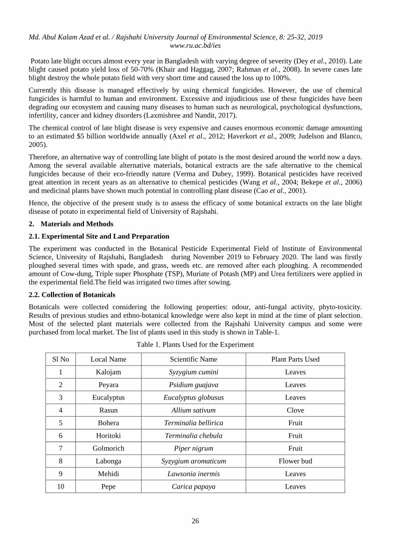
Md. Abul Kalam Azad et al. / Rajshahi University Journal of Environmental Science, 8: 25-32, 2019 www.ru.ac.bd/ies
26
Potato late blight occurs almost every year in Bangladesh with varying degree of severity (Dey et al., 2010). Late blight caused potato yield loss of 50-70% (Khair and Haggag, 2007; Rahman et al., 2008). In severe cases late blight destroy the whole potato field with very short time and caused the loss up to 100%.
Currently this disease is managed effectively by using chemical fungicides. However, the use of chemical fungicides is harmful to human and environment. Excessive and injudicious use of these fungicides have been degrading our ecosystem and causing many diseases to human such as neurological, psychological dysfunctions, infertility, cancer and kidney disorders (Laxmishree and Nandit, 2017).
The chemical control of late blight disease is very expensive and causes enormous economic damage amounting to an estimated $5 billion worldwide annually (Axel et al., 2012; Haverkort et al., 2009; Judelson and Blanco, 2005).
Therefore, an alternative way of controlling late blight of potato is the most desired around the world now a days. Among the several available alternative materials, botanical extracts are the safe alternative to the chemical fungicides because of their eco-friendly nature (Verma and Dubey, 1999). Botanical pesticides have received great attention in recent years as an alternative to chemical pesticides (Wang et al., 2004; Bekepe et al., 2006) and medicinal plants have shown much potential in controlling plant disease (Cao et al., 2001).
Hence, the objective of the present study is to assess the efficacy of some botanical extracts on the late blight disease of potato in experimental field of University of Rajshahi.
2. Materials and Methods
2.1. Experimental Site and Land Preparation
The experiment was conducted in the Botanical Pesticide Experimental Field of Institute of Environmental Science, University of Rajshahi, Bangladesh during November 2019 to February 2020. The land was firstly ploughed several times with spade, and grass, weeds etc. are removed after each ploughing. A recommended amount of Cow-dung, Triple super Phosphate (TSP), Muriate of Potash (MP) and Urea fertilizers were applied in the experimental field.The field was irrigated two times after sowing.
2.2. Collection of Botanicals
Botanicals were collected considering the following properties: odour, anti-fungal activity, phyto-toxicity. Results of previous studies and ethno-botanical knowledge were also kept in mind at the time of plant selection. Most of the selected plant materials were collected from the Rajshahi University campus and some were purchased from local market. The list of plants used in this study is shown in Table-1.
Table 1. Plants Used for the Experiment
Sl No Local Name Scientific Name Plant Parts Used 1 Kalojam Syzygium cumini Leaves 2 Peyara Psidium guajava Leaves 3 Eucalyptus Eucalyptus globusus Leaves 4 Rasun Allium sativum Clove 5 Bohera Terminalia bellirica Fruit 6 Horitoki Terminalia chebula Fruit 7 Golmorich Piper nigrum Fruit 8 Labonga Syzygium aromaticum Flower bud 9 Mehidi Lawsonia inermis Leaves 10 Pepe Carica papaya Leaves
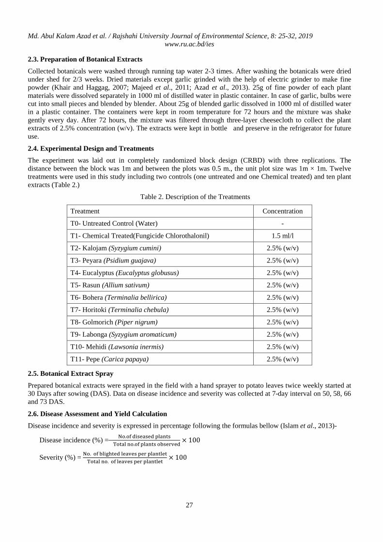
Md. Abul Kalam Azad et al. / Rajshahi University Journal of Environmental Science, 8: 25-32, 2019 www.ru.ac.bd/ies
27
2.3. Preparation of Botanical Extracts
Collected botanicals were washed through running tap water 2-3 times. After washing the botanicals were dried under shed for 2/3 weeks. Dried materials except garlic grinded with the help of electric grinder to make fine powder (Khair and Haggag, 2007; Majeed et al., 2011; Azad et al., 2013). 25g of fine powder of each plant materials were dissolved separately in 1000 ml of distilled water in plastic container. In case of garlic, bulbs were cut into small pieces and blended by blender. About 25g of blended garlic dissolved in 1000 ml of distilled water in a plastic container. The containers were kept in room temperature for 72 hours and the mixture was shake gently every day. After 72 hours, the mixture was filtered through three-layer cheesecloth to collect the plant extracts of 2.5% concentration (w/v). The extracts were kept in bottle and preserve in the refrigerator for future use.
2.4. Experimental Design and Treatments
The experiment was laid out in completely randomized block design (CRBD) with three replications. The distance between the block was 1m and between the plots was 0.5 m., the unit plot size was 1m × 1m. Twelve treatments were used in this study including two controls (one untreated and one Chemical treated) and ten plant extracts (Table 2.)
Table 2. Description of the Treatments
Treatment Concentration
T0- Untreated Control (Water) -
T1- Chemical Treated(Fungicide Chlorothalonil) 1.5 ml/l
T2- Kalojam (Syzygium cumini) 2.5% (w/v)
T3- Peyara (Psidium guajava) 2.5% (w/v)
T4- Eucalyptus (Eucalyptus globusus) 2.5% (w/v)
T5- Rasun (Allium sativum) 2.5% (w/v)
T6- Bohera (Terminalia bellirica) 2.5% (w/v)
T7- Horitoki (Terminalia chebula) 2.5% (w/v)
T8- Golmorich (Piper nigrum) 2.5% (w/v)
T9- Labonga (Syzygium aromaticum) 2.5% (w/v)
T10- Mehidi (Lawsonia inermis) 2.5% (w/v)
T11- Pepe (Carica papaya) 2.5% (w/v)
2.5. Botanical Extract Spray
Prepared botanical extracts were sprayed in the field with a hand sprayer to potato leaves twice weekly started at 30 Days after sowing (DAS). Data on disease incidence and severity was collected at 7-day interval on 50, 58, 66 and 73 DAS.
2.6. Disease Assessment and Yield Calculation
Disease incidence and severity is expressed in percentage following the formulas bellow (Islam et al., 2013)-
Disease incidence (%) = No.of diseased plants Total no.of plants observed
× 100
Severity (%) = No. of blighted leaves per plantletTotal no. of leaves per plantlet
× 100
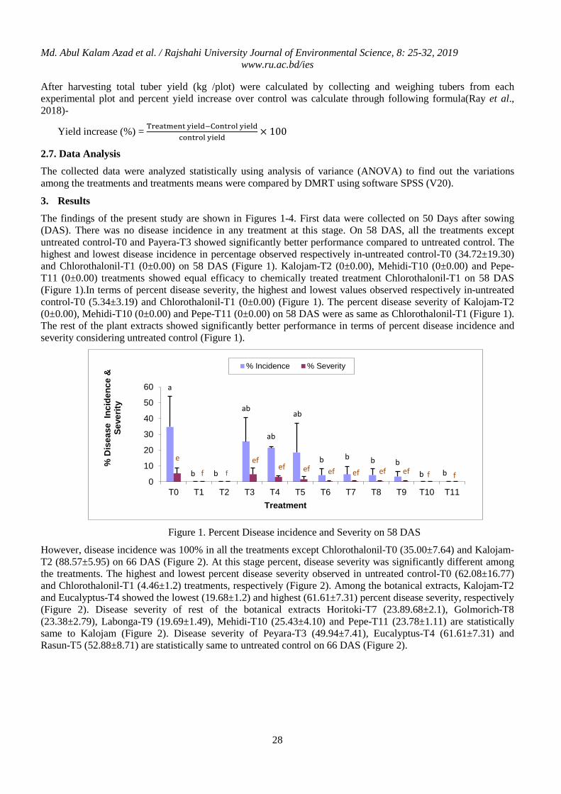
Md. Abul Kalam Azad et al. / Rajshahi University Journal of Environmental Science, 8: 25-32, 2019 www.ru.ac.bd/ies
28
After harvesting total tuber yield (kg /plot) were calculated by collecting and weighing tubers from each experimental plot and percent yield increase over control was calculate through following formula(Ray et al., 2018)-
Yield increase (%) = Treatment yield−Control yieldcontrol yield
× 100
2.7. Data Analysis
The collected data were analyzed statistically using analysis of variance (ANOVA) to find out the variations among the treatments and treatments means were compared by DMRT using software SPSS (V20).
3. Results
The findings of the present study are shown in Figures 1-4. First data were collected on 50 Days after sowing (DAS). There was no disease incidence in any treatment at this stage. On 58 DAS, all the treatments except untreated control-T0 and Payera-T3 showed significantly better performance compared to untreated control. The highest and lowest disease incidence in percentage observed respectively in-untreated control-T0 (34.72±19.30) and Chlorothalonil-T1 (0±0.00) on 58 DAS (Figure 1). Kalojam-T2 (0±0.00), Mehidi-T10 (0±0.00) and Pepe-T11 (0±0.00) treatments showed equal efficacy to chemically treated treatment Chlorothalonil-T1 on 58 DAS (Figure 1).In terms of percent disease severity, the highest and lowest values observed respectively in-untreated control-T0 (5.34±3.19) and Chlorothalonil-T1 (0±0.00) (Figure 1). The percent disease severity of Kalojam-T2 (0±0.00), Mehidi-T10 (0±0.00) and Pepe-T11 (0±0.00) on 58 DAS were as same as Chlorothalonil-T1 (Figure 1). The rest of the plant extracts showed significantly better performance in terms of percent disease incidence and severity considering untreated control (Figure 1).
Figure 1. Percent Disease incidence and Severity on 58 DAS
However, disease incidence was 100% in all the treatments except Chlorothalonil-T0 (35.00±7.64) and Kalojam-T2 (88.57±5.95) on 66 DAS (Figure 2). At this stage percent, disease severity was significantly different among the treatments. The highest and lowest percent disease severity observed in untreated control-T0 (62.08±16.77) and Chlorothalonil-T1 (4.46±1.2) treatments, respectively (Figure 2). Among the botanical extracts, Kalojam-T2 and Eucalyptus-T4 showed the lowest (19.68±1.2) and highest (61.61±7.31) percent disease severity, respectively (Figure 2). Disease severity of rest of the botanical extracts Horitoki-T7 (23.89.68±2.1), Golmorich-T8 (23.38±2.79), Labonga-T9 (19.69±1.49), Mehidi-T10 (25.43±4.10) and Pepe-T11 (23.78±1.11) are statistically same to Kalojam (Figure 2). Disease severity of Peyara-T3 (49.94±7.41), Eucalyptus-T4 (61.61±7.31) and Rasun-T5 (52.88±8.71) are statistically same to untreated control on 66 DAS (Figure 2).
0
10
20
30
40
50
60
T0 T1 T2 T3 T4 T5 T6 T7 T8 T9 T10 T11
% D
isea
se I
ncid
ence
&
Seve
rity
Treatment
% Incidence % Severity
a
b b
ab
b b b b
b b
ab
ab
e
f f
ef ef ef ef ef ef f
f ef
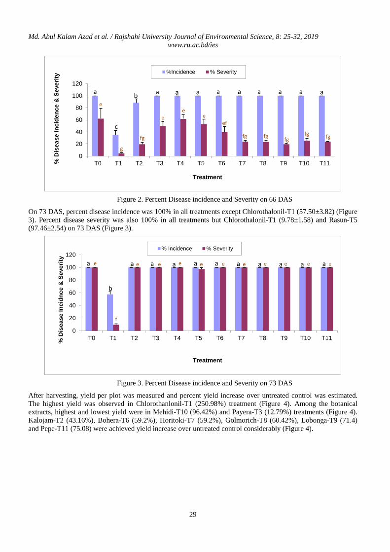
Md. Abul Kalam Azad et al. / Rajshahi University Journal of Environmental Science, 8: 25-32, 2019 www.ru.ac.bd/ies
29
Figure 2. Percent Disease incidence and Severity on 66 DAS
On 73 DAS, percent disease incidence was 100% in all treatments except Chlorothalonil-T1 (57.50±3.82) (Figure 3). Percent disease severity was also 100% in all treatments but Chlorothalonil-T1 (9.78±1.58) and Rasun-T5 (97.46±2.54) on 73 DAS (Figure 3).
Figure 3. Percent Disease incidence and Severity on 73 DAS
After harvesting, yield per plot was measured and percent yield increase over untreated control was estimated. The highest yield was observed in Chlorothanlonil-T1 (250.98%) treatment (Figure 4). Among the botanical extracts, highest and lowest yield were in Mehidi-T10 (96.42%) and Payera-T3 (12.79%) treatments (Figure 4). Kalojam-T2 (43.16%), Bohera-T6 (59.2%), Horitoki-T7 (59.2%), Golmorich-T8 (60.42%), Lobonga-T9 (71.4) and Pepe-T11 (75.08) were achieved yield increase over untreated control considerably (Figure 4).
0
20
40
60
80
100
120
T0 T1 T2 T3 T4 T5 T6 T7 T8 T9 T10 T11% D
isea
se In
cide
nce
& S
ever
ity
Treatment
%Incidence % Severity
a a a a a a a
e
e e
e
b
g
fg
ef
fg fg fg fg fg
c
a a a
0
20
40
60
80
100
120
T0 T1 T2 T3 T4 T5 T6 T7 T8 T9 T10 T11% D
isea
se In
cidn
ce &
Sev
erity
Treatment
% Incidence % Severity
a a a a a a a a a a a
b
e e e e e e e e e e e
f
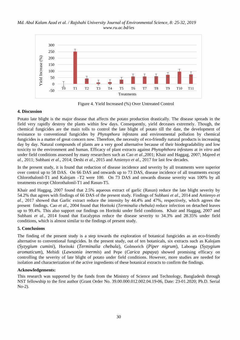
Md. Abul Kalam Azad et al. / Rajshahi University Journal of Environmental Science, 8: 25-32, 2019 www.ru.ac.bd/ies
30
Figure 4. Yield Increased (%) Over Untreated Control
4. Discussion
Potato late blight is the major disease that affects the potato production drastically. The disease spreads in the field very rapidly destroy the plants within few days. Consequently, yield deceases extremely. Though, the chemical fungicides are the main tolls to control the late blight of potato till the date, the development of resistance to conventional fungicides by Phytopthora infestans and environmental pollution by chemical fungicides is a matter of great concern now. Therefore, the necessity of eco-friendly natural products is increasing day by day. Natural compounds of plants are a very good alternative because of their biodegradability and low toxicity to the environment and human. Efficacy of plant extracts against Phytophthora infestans at in vitro and under field conditions assessed by many researchers such as Cao et al.,2001; Khair and Haggag, 2007; Majeed et al., 2011; Subhani et al., 2014; Deshi et al., 2015 and Amienyo et al., 2017 for last few decades.
In the present study, it is found that reduction of disease incidence and severity by all treatments were superior over control up to 58 DAS. On 66 DAS and onwards up to 73 DAS, disease incidence of all treatments except Chlorothalonil-T1 and Kalojam –T2 were 100. On 73 DAS and onwards disease severity was 100% by all treatments except Chlorothalonil-T1 and Rasun-T5.
Khair and Haggag, 2007 found that 2.5% aqueous extract of garlic (Rasun) reduce the late blight severity by 54.2% that agrees with findings of 66 DAS of the present study. Findings of Subhani et al., 2014 and Amienyo et al., 2017 showed that Garlic extract reduce the intensity by 44.4% and 47%, respectively, which agrees the present findings. Cao et al., 2004 found that Horitoki (Terminalia chebula) reduce infection on detached leaves up to 99.4%. This also support our findings on Horitoki under field conditions. Khair and Haggag, 2007 and Subhani et al., 2014 found that Eucalyptus reduce the disease severity to 34.3% and 28.35% under field conditions, which is almost similar to the findings of present study.
5. Conclusions
The finding of the present study is a step towards the exploration of botanical fungicides as an eco-friendly alternative to conventional fungicides. In the present study, out of ten botanicals, six extracts such as Kalojam (Syzygium cumini), Horitoki (Terminalia chebula), Golmorich (Piper nigrum), Labonga (Syzygium aromaticum), Mehidi (Lawsonia inermis) and Pepe (Carica papaya) showed promising efficacy on controlling the severity of late blight of potato under field conditions. However, more studies are needed for isolation and characterization of the active ingredients of these botanical extracts to confirm the findings.
Acknowledgements: This research was supported by the funds from the Ministry of Science and Technology, Bangladesh through NST fellowship to the first author (Grant Order No. 39.00.000.012.002.04.19-06, Date: 23-01.2020; Ph.D. Serial No-2).
-500
50100150200250300
T0 T1 T2 T3 T4 T5 T6 T7 T8 T9 T10 T11
Yie
ld In
crea
se (%
)
Treatments
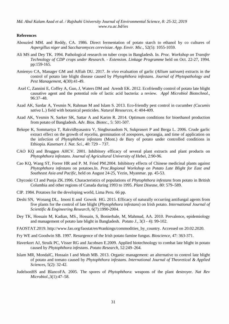
Md. Abul Kalam Azad et al. / Rajshahi University Journal of Environmental Science, 8: 25-32, 2019 www.ru.ac.bd/ies
31
References
Abouzied MM. and Reddy, CA. 1986. Direct fermentation of potato starch to ethanol by co cultures of Aspergillus niger and Saccharomyces cerevisiae. App. Envir. Mic., 52(5): 1055-1059.
Ali MS and Dey TK. 1994. Pathological research on tuber crops in Bangladesh. In. Proc. Workshop on Transfer Technology of CDP crops under Research. - Extension. Linkage Programme held on Oct. 22-27, 1994. pp:159-165.
Amienyo CA, Manager GM and Affiah DU. 2017. In vivo evaluation of garlic (Allium sativum) extracts in the control of potato late blight disease caused by Phytophthora infestans. Journal of Phytopathology and Pest Management, 4(30):41-49.
Axel C, Zannini E, Coffey A, Guo, J, Waters DM and Arendt EK. 2012. Ecofriendly control of potato late blight causative agent and the potential role of lactic acid bacteria: a review. Appl Microbiol Biotechnol., 96:37–48.
Azad AK, Sardar A, Yesmin N, Rahman M and Islam S. 2013. Eco-friendly pest control in cucumber (Cucumis sativa L.) field with botanical pesticides. Natural Resources, 4: 404-409.
Azad AK, Yesmin N, Sarker SK, Sattar A and Karim R. 2014. Optimum conditions for bioethanol production from potato of Bangladesh. Adv. Bios. Biotec., 5: 501-507.
Bekepe K, Sommartya T, Rakvidhyasastra V, Singburaudom N, Sukprasert P and Berga L. 2006. Crude garlic extract effect on the growth of mycelia, germination of zoospores, sporangia, and time of application on the infection of Phytophthora infestans (Mont.) de Bary of potato under controlled conditions in Ethiopia. Kasetsart J. Nat. Sci., 40: 729 – 737.
CAO KQ and Bruggen AHCV. 2001. Inhibitory efficacy of several plant extracts and plant products on Phytophthora infestans. Journal of Agricultural University of Hebei, 2:90-96.
Cao KQ, Wang ST, Forrer HR and P. M. Fried PM.2004. Inhibitory effects of Chinese medicinal plants against Phytophthora infestans on potatoes.In. Proc.Regional Workshop on Potato Late Blight for East and Southeast Asia and Pacific, held on August 24-25, Yezin, Myanmar. pp. 45-53.
Chycoski CI and Punja ZK.1996. Characteristics of populations of Phytophthora infestans from potato in British Columbia and other regions of Canada during 1993 to 1995. Plant Disease, 80: 579–589.
CIP. 1984. Potatoes for the developing world, Lima Peru. 66 pp.
Deshi SN, Wonang DL, Imoni E and Gowok HG. 2015. Efficacy of naturally occurring antifungal agents from five plants for the control of late blight (Phytophthora infestans) on Irish potato. International Journal of Scientific & Engineering Research, 6(7):1990-2004.
Dey TK, Hossain M, Kadian, MS., Hossain, S, Bonierbale, M, Mahmud, AA. 2010. Prevalence, epidemiology and management of potato late blight in Bangladesh. Potato J., 3(3 - 4): 99-102.
FAOSTAT.2019. http://www.fao.org/faostat/en/#rankings/commodities_by_country. Accessed on 20.02.2020.
Fry WE and Goodwin SB. 1997. Resurgence of the Irish potato famine fungus. Bioscience, 47: 363-371.
Haverkort AJ, Struik PC, Visser RG and Jacobsen E.2009. Applied biotechnology to combat late blight in potato caused by Phytophthora infestans. Potato Research, 52:249–264.
Islam MR, MondalC, Hossain I and Meah MB. 2013. Organic management: an alternative to control late blight of potato and tomato caused by Phytophthora infestans. International Journal of Theoretical & Applied Sciences, 5(2): 32-42.
JudelsonHS and BlancoFA. 2005. The spores of Phytophthora: weapons of the plant destroyer. Nat Rev Microbiol.,3(1):47–58.
Md. Abul Kalam Azad et al. / Rajshahi University Journal of Environmental Science, 8: 25-32, 2019 www.ru.ac.bd/ies
32
Khair Abd-El and Haggag WM. 2007. Application of some Egyptian medicinal plant extracts against potato late and early blights. Research Journal of Agriculture and Biological Sciences, 3(3):166-175.
King JC and Slavin JL. 2013. White potatoes, human health, and dietary guidance. Adv. Nutr., 4(3): 393-401.
Laxmishree and Nandit. 2017. Botanical pesticides – a major alternative to chemical pesticides: a review. Int. J. of Life Sciences, 5 (4): 722-729.
Majeed A, Ahmad H, Chaudhry Z , Jan G, Alam J and Muhammad Z. 2011. Assessment of leaf extracts of three medicinal plants against late blight of potato in Kaghan valley, Pakistan. Journal of Agricultural Technology, 7(4): 1155-1161.
Rahman MM, Dey TK, Ali MA, Khalequzzaman KM and Hussain MA. 2008. Control of late blight disease of potato by using new fungicides. Int. J. Sustain. Crop Prod., 3(2):10-15.
Ray PK, Singh HK, Chaudhary A and Verma RB.2018. Effect of certain fungicides and botanicals against late blight of potato (Phytophthora infestans). Current Journal of Applied Science and Technology31(3): 1-5.
Singha U and Maezawa S. 2019. Production, marketing system, storage and future aspect of potato in Bangladesh. Reviews in Agricultural Science, 7:29-40.
Subhani MN, Sahi ST, Hussain S, Munir N, Abbas W and Bilal M. 2014. Evaluation of antifungal effect of different plant extracts for the management of late blight of potato caused by Phytophthora infestans (Mont.) de Bary. TBAP., 4 (2): 125–135.
Varma J and Dubey NK. 1999. Prospectives of botanical and microbial products as pesticides of tomorrow. Current Science, 76 (2):172-179.
Wang S, Hu T, Zhang F, Zhen W, Song P, Forrer HR and Cao K. 2004 . Screening for alternate Products to control potato late blight. In. Proc. Regional Workshop on Potato Late Blight for East and Southeast Asia and Pacific, held on August 24-25, Yezin, Myanmar. pp. 68-73.
Bayezid Mahmud Khan et al. / Rajshahi University Journal of Environmental Science, 8: 33-42, 2019 www.ru.ac.bd/ies
Germination and Seedling Growth Performance of Benincasa hispida (Thunb.) Cogn. in Arsenic Solution Cultures under Phosphorus Amendment
Bayezid Mahmud Khan1∗, Afroza Hasan Afrin1, Mohammad Mosharraf Hossain1 and Ismail Md.
Mofizur Rahman2
1Institute of Forestry and Environmental Sciences, University of Chittagong, Chittagong-4331, Bangladesh 2Institute of Environmental Radioactivity, Fukushima University, Fukushima 960-1296, Japan
Abstract
Arsenic (As) is a toxic metalloid widely distributed in the environment posing a serious threat to human health. Based on past studies, it was postulated that enriching the soil with phosphorus (P) is an option to offset the negative effects of As on plant growth. However, attempts towards finding the precise role of P are limited. This study, therefore, aimed to determine the efficacy of P in balancing the negative effects of As on Benincasa hispida as measured in terms of seed germination, seedling growth and biomass production of seedling. Seeds of B. hispida were treated with different concentrations (2 ppm, 5 ppm and 10 ppm) of As, with or without addition of P (10 ppm). As exposure hindered germination rate, seedling growth and biomass production of seedling to different magnitudes depending on the concentrations. Addition of P in As solution cultures improved the seed and seedling performance significantly. Germination were 91% in 2 ppm As+10 ppm P, 85% in ppm As+10 ppm P and 74% in 10 ppm As+10 ppm P compared to 89% in 2 ppm As, 79% in 5 ppm As and 67% in 10 ppm As. In treatments T1 2 ppm As, T3 5 ppm As and 10 ppm As, seedling dry biomasses were 24 mg, 12 mg and 10 mg respectively, which were enhanced to 27 mg, 19 mg and 15 mg respectively in 2 ppm As+10 ppm P, 5 ppm As+10 ppm P and 10 ppm As+10 ppm P. Similar trend was also recorded for plumule growth, seedling fresh biomass production, seedling vigor, sturdiness etc. This study, therefore, recommended the application of P to reduce the negative effects of As on B. hispida in As solution culture under laboratory condition and maintains that the results may hold good in the field condition as well.
Keywords: Arsenic; Benincasa hispida; Germination; Phosphorus; Seedling vigor; Sturdiness.
1. Introduction
Native to South Asia and Southeast Asia including Bangladesh - Benincasa hispida (Thunb.) Cogn., the wax gourd, also known as winter melon, is widely grown throughout Asia, including Java and Japan where it is thought to have originated (Bimakr et al., 2016). It is belong to the horticulturally diverse gourd family Cucurbitaceae and only member of the genus Benincasa. Wax gourd is a vine grown for its very large fruit, eaten as a vegetable when mature. The fruit is fuzzy when young and has thick white flesh that is sweet. By maturity, the fruit loses its hairs and develops a waxy coating and providing a long shelf life (Rayees et al., 2013). It is grown in well drained loam and sandy soils, in warm mild climates, but will not tolerate frosts. The crops are grown in riverbeds or furrows, and needs constant irrigation during the growing season (Rayees et al., 2013; Bimakr et al., 2016).
In Bangladesh, elevated concentration of arsenic (As) in the surface soil of agricultural field and in plant tissue were reported since As contaminated groundwater has been used for irrigation (Meharg and Rahman, 2003). Areas under wax gourd cultivation in Bangladesh are prone to the risk. Being a toxic element, As poses serious threats to environment and human health (Leimu and Fischer, 2008; Singh et al., 2015; Babst-Kostecka et al., 2016; Guevara-Garcia et al., 2017; Khan et al., 2018). When crops are grown in As-contaminated soil or irrigated with As-contaminated water, As gets accumulated in the seeds or grain which is becoming an increasingly important problem in many parts of the world (Sanal et al., 2014) as it poses significant risk to animal and human health through soil-crop transfer (Fitz and Wenzel, 2002; Sultana et al., 2015). At high level of As concentrations, biomass production and yields of a variety of crops shrink significantly (Carbonell-Barrachina et al., 1997; Chaturvedi, 2006). Especially, plants with highly water-retentive fruits, such as wax gourd, accumulates As in elevated concentrations in their fruit (Mishra et al., 2014). Melons including wax gourd, however, is naturally efficient in preventing As accumulation in the fruit (Hettick, 2016).
∗ Corresponding author’s e-mail: [email protected]
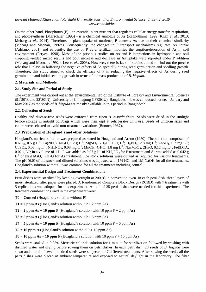
Bayezid Mahmud Khan et al. / Rajshahi University Journal of Environmental Science, 8: 33-42, 2019 www.ru.ac.bd/ies
34
On the other hand, Phosphorus (P) - an essential plant nutrient that regulates cellular energy transfer, respiration, and photosynthesis (Marschner, 1995) - is a chemical analogue of As (Raghothama, 1999; Khan et al., 2013; Meharg et al., 2014). Therefore, in plant uptake of nutrients, P contests As due to their chemical similarity (Meharg and Macnair, 1992a). Consequently, the changes in P transport mechanisms regulates As uptake (Adriano, 2001) and evidently, the use of P as a fertilizer modifies the sorption/desorption of As in soil environment (Peryea, 1998). Most of the previous studies on As and P interactions in hydroponic and soil cropping yielded mixed results and both increase and decrease in As uptake were reported under P addition (Meharg and Macnair, 1992b; Lee et al., 2003). However, there is lack of studies aimed to find out the precise role that P plays in buffering the negative effects of As specially during seed germination and seedling growth. Therefore, this study aimed to check the efficacy of P in reducing the negative effects of As during seed germination and initial seedling growth in terms of biomass production of B. hispida.
2. Materials and Methods
2.1. Study Site and Period of Study
The experiment was carried out at the environmental lab of the Institute of Forestry and Environmental Sciences (91050´E and 22030´N), University of Chittagong (IFESCU), Bangladesh. It was conducted between January and May 2017 as the seeds of B. hispida are mostly available in this period in Bangladesh.
2.2. Collection of Seeds
Healthy and disease-free seeds were extracted from ripen B. hispida fruits. Seeds were dried in the sunlight before storage in airtight polybags which were then kept at refrigerator until use. Seeds of uniform sizes and colors were selected to avoid non-treatment variations (Bonner, 1987).
2.3. Preparation of Hoagland’s and other Solutions
Hoagland’s nutrient solution was prepared as stated in Hoagland and Arnon (1950). The solution comprised of KNO3, 0.5 g L-1; Ca(NO3). 4H2O, 1.2 g L-1; MgSO4. 7H2O, 0.5 g L-1; H3BO3, 2.8 mg L-1; ZnSO4, 0.2 mg L-1; CuSO4, 0.05 mg L-1; NH4NO3, 0.08 mg L-1; MnCl2. 4H2O, 1.8 mg L-1; Na2MoO4. 2H2O, 0.12 mg L-1; FeEDTA, 0.02 g L-1; in a volume of 1 L. P was added as 0.07 g L-1 of KH2PO4 for P treatment and As was added as 0.042 g L-1 of Na2HAsO4. 7H2O for As treatment. The stock solutions were diluted as required for various treatments. The pH (6.0) of the stock and diluted solutions was adjusted with 1M HCl and 1M NaOH for all the treatments. Hoagland’s solution without P was common for all the treatments including control.
2.4. Experimental Design and Treatment Combinations
Petri dishes were sterilized by keeping overnight at 200 0C in convection oven. In each petri dish, three layers of moist sterilized filter paper were placed. A Randomized Complete Block Design (RCBD) with 7 treatments with 5 replications was adopted for this experiment. A total of 35 petri dishes were needed for this experiment. The treatment combinations used in the experiment were:
T0 = Control (Hoagland’s solution without P)
T1 = 2 ppm As (Hoagland’s solution without P + 2 ppm As)
T2 = 2 ppm As + 10 ppm P (Hoagland’s solution with 10 ppm P + 2 ppm As)
T3 = 5 ppm As (Hoagland’s solution without P + 5 ppm As)
T4 = 5 ppm As + 10 ppm P (Hoagland’s solution with 10 ppm P + 5 ppm As)
T5 = 10 ppm As (Hoagland’s solution without P + 10 ppm As)
T6 = 10 ppm As + 10 ppm P (Hoagland’s solution with 10 ppm P + 10 ppm As)
Seeds were soaked in 0.05% Mercuric chloride solution for 1 minute for sterilization followed by washing with distilled water and drying before sowing them on petri dishes. In each petri dish, 20 seeds of B. hispida were sown and a total of seven hundred seeds were subjected to 7 different treatments. After sowing the seeds, all the petri dishes were placed at ambient temperature and exposed to natural daylight in the laboratory. The filter
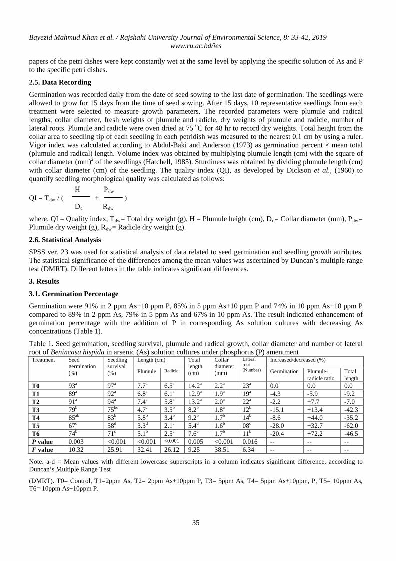
Bayezid Mahmud Khan et al. / Rajshahi University Journal of Environmental Science, 8: 33-42, 2019 www.ru.ac.bd/ies
35
papers of the petri dishes were kept constantly wet at the same level by applying the specific solution of As and P to the specific petri dishes.
2.5. Data Recording
Germination was recorded daily from the date of seed sowing to the last date of germination. The seedlings were allowed to grow for 15 days from the time of seed sowing. After 15 days, 10 representative seedlings from each treatment were selected to measure growth parameters. The recorded parameters were plumule and radical lengths, collar diameter, fresh weights of plumule and radicle, dry weights of plumule and radicle, number of lateral roots. Plumule and radicle were oven dried at 75 0C for 48 hr to record dry weights. Total height from the collar area to seedling tip of each seedling in each petridish was measured to the nearest 0.1 cm by using a ruler. Vigor index was calculated according to Abdul-Baki and Anderson (1973) as germination percent × mean total (plumule and radical) length. Volume index was obtained by multiplying plumule length (cm) with the square of collar diameter (mm)2 of the seedlings (Hatchell, 1985). Sturdiness was obtained by dividing plumule length (cm) with collar diameter (cm) of the seedling. The quality index (QI), as developed by Dickson et al., (1960) to quantify seedling morphological quality was calculated as follows: H Pdw QI = Tdw / ( + ) Dc Rdw
where, QI = Quality index, Tdw= Total dry weight (g), H = Plumule height (cm), Dc= Collar diameter (mm), Pdw= Plumule dry weight (g), Rdw= Radicle dry weight (g).
2.6. Statistical Analysis
SPSS ver. 23 was used for statistical analysis of data related to seed germination and seedling growth attributes. The statistical significance of the differences among the mean values was ascertained by Duncan’s multiple range test (DMRT). Different letters in the table indicates significant differences.
3. Results
3.1. Germination Percentage
Germination were 91% in 2 ppm As+10 ppm P, 85% in 5 ppm As+10 ppm P and 74% in 10 ppm As+10 ppm P compared to 89% in 2 ppm As, 79% in 5 ppm As and 67% in 10 ppm As. The result indicated enhancement of germination percentage with the addition of P in corresponding As solution cultures with decreasing As concentrations (Table 1).
Table 1. Seed germination, seedling survival, plumule and radical growth, collar diameter and number of lateral root of Benincasa hispida in arsenic (As) solution cultures under phosphorus (P) amentment
Treatment Seed germination (%)
Seedling survival (%)
Length (cm) Total length (cm)
Collar diameter (mm)
Lateral root (Number)
Increased/decreased (%)
Plumule Radicle Germination Plumule-radicle ratio
Total length
T0 93a 97a 7.7a 6.5a 14.2a 2.2a 23a 0.0 0.0 0.0 T1 89a 92a 6.8a 6.1a 12.9a 1.9a 19a -4.3 -5.9 -9.2 T2 91a 94a 7.4a 5.8a 13.2a 2.0a 22a -2.2 +7.7 -7.0 T3 79b 75bc 4.7c 3.5b 8.2b 1.8a 12b -15.1 +13.4 -42.3 T4 85ab 83b 5.8b 3.4b 9.2b 1.7b 14b -8.6 +44.0 -35.2 T5 67c 58d 3.3d 2.1c 5.4d 1.6b 08c -28.0 +32.7 -62.0 T6 74b 71c 5.1b 2.5c 7.6c 1.7b 11b -20.4 +72.2 -46.5 P value 0.003 <0.001 <0.001 <0.001 0.005 <0.001 0.016 -- -- -- F value 10.32 25.91 32.41 26.12 9.25 38.51 6.34 -- -- --
Note: a-d = Mean values with different lowercase superscripts in a column indicates significant difference, according to Duncan’s Multiple Range Test
(DMRT). T0= Control, T1=2ppm As, T2= 2ppm As+10ppm P, T3= 5ppm As, T4= 5ppm As+10ppm, P, T5= 10ppm As, T6= 10ppm As+10ppm P.
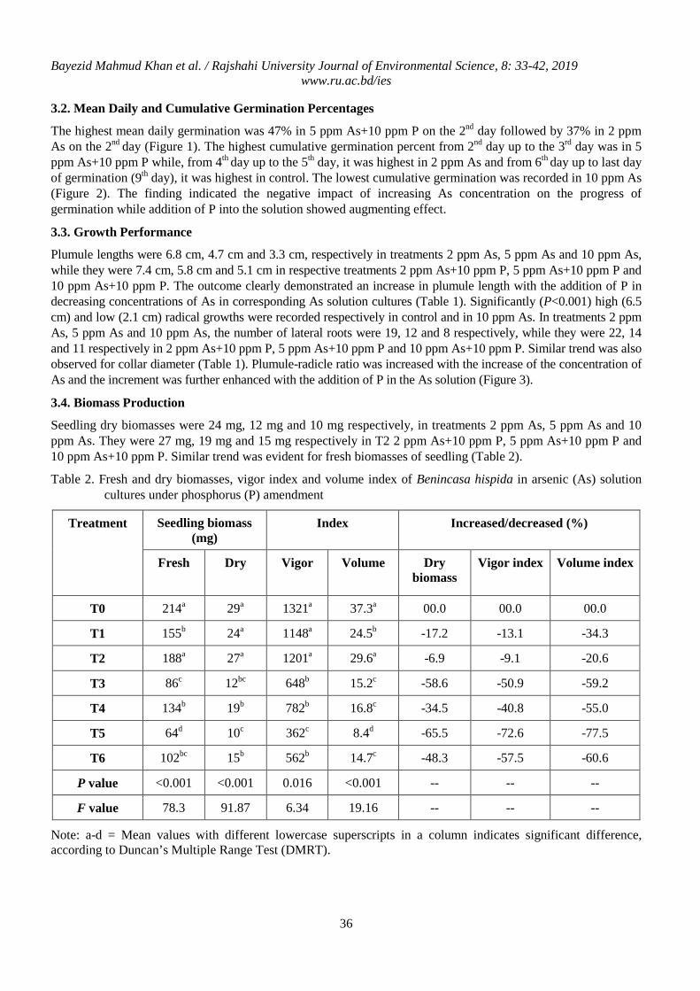
Bayezid Mahmud Khan et al. / Rajshahi University Journal of Environmental Science, 8: 33-42, 2019 www.ru.ac.bd/ies
36
3.2. Mean Daily and Cumulative Germination Percentages
The highest mean daily germination was 47% in 5 ppm As+10 ppm P on the 2nd day followed by 37% in 2 ppm As on the 2nd day (Figure 1). The highest cumulative germination percent from 2nd day up to the 3rd day was in 5 ppm As+10 ppm P while, from 4th day up to the 5th day, it was highest in 2 ppm As and from 6th day up to last day of germination (9th day), it was highest in control. The lowest cumulative germination was recorded in 10 ppm As (Figure 2). The finding indicated the negative impact of increasing As concentration on the progress of germination while addition of P into the solution showed augmenting effect.
3.3. Growth Performance
Plumule lengths were 6.8 cm, 4.7 cm and 3.3 cm, respectively in treatments 2 ppm As, 5 ppm As and 10 ppm As, while they were 7.4 cm, 5.8 cm and 5.1 cm in respective treatments 2 ppm As+10 ppm P, 5 ppm As+10 ppm P and 10 ppm As+10 ppm P. The outcome clearly demonstrated an increase in plumule length with the addition of P in decreasing concentrations of As in corresponding As solution cultures (Table 1). Significantly (P<0.001) high (6.5 cm) and low (2.1 cm) radical growths were recorded respectively in control and in 10 ppm As. In treatments 2 ppm As, 5 ppm As and 10 ppm As, the number of lateral roots were 19, 12 and 8 respectively, while they were 22, 14 and 11 respectively in 2 ppm As+10 ppm P, 5 ppm As+10 ppm P and 10 ppm As+10 ppm P. Similar trend was also observed for collar diameter (Table 1). Plumule-radicle ratio was increased with the increase of the concentration of As and the increment was further enhanced with the addition of P in the As solution (Figure 3).
3.4. Biomass Production
Seedling dry biomasses were 24 mg, 12 mg and 10 mg respectively, in treatments 2 ppm As, 5 ppm As and 10 ppm As. They were 27 mg, 19 mg and 15 mg respectively in T2 2 ppm As+10 ppm P, 5 ppm As+10 ppm P and 10 ppm As+10 ppm P. Similar trend was evident for fresh biomasses of seedling (Table 2).
Table 2. Fresh and dry biomasses, vigor index and volume index of Benincasa hispida in arsenic (As) solution cultures under phosphorus (P) amendment
Treatment Seedling biomass (mg)
Index Increased/decreased (%)
Fresh Dry Vigor Volume
Dry biomass
Vigor index Volume index
T0 214a 29a 1321a 37.3a 00.0 00.0 00.0
T1 155b 24a 1148a 24.5b -17.2 -13.1 -34.3
T2 188a 27a 1201a 29.6a -6.9 -9.1 -20.6
T3 86c 12bc 648b 15.2c -58.6 -50.9 -59.2
T4 134b 19b 782b 16.8c -34.5 -40.8 -55.0
T5 64d 10c 362c 8.4d -65.5 -72.6 -77.5
T6 102bc 15b 562b 14.7c -48.3 -57.5 -60.6
P value <0.001 <0.001 0.016 <0.001 -- -- --
F value 78.3 91.87 6.34 19.16 -- -- --
Note: a-d = Mean values with different lowercase superscripts in a column indicates significant difference, according to Duncan’s Multiple Range Test (DMRT).
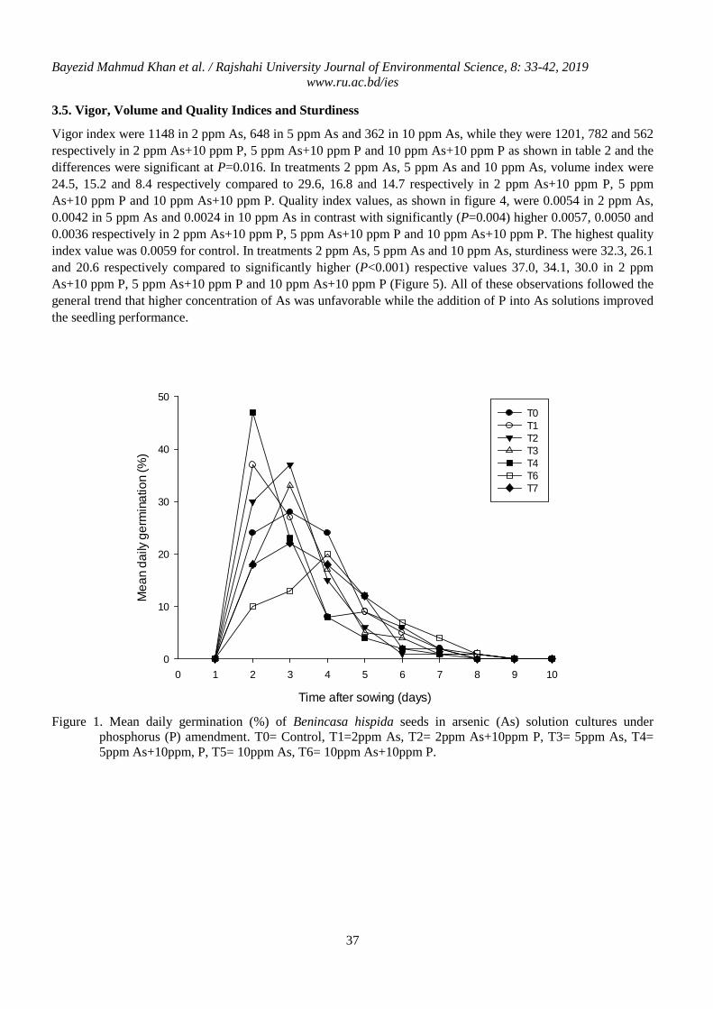
Bayezid Mahmud Khan et al. / Rajshahi University Journal of Environmental Science, 8: 33-42, 2019 www.ru.ac.bd/ies
37
3.5. Vigor, Volume and Quality Indices and Sturdiness
Vigor index were 1148 in 2 ppm As, 648 in 5 ppm As and 362 in 10 ppm As, while they were 1201, 782 and 562 respectively in 2 ppm As+10 ppm P, 5 ppm As+10 ppm P and 10 ppm As+10 ppm P as shown in table 2 and the differences were significant at P=0.016. In treatments 2 ppm As, 5 ppm As and 10 ppm As, volume index were 24.5, 15.2 and 8.4 respectively compared to 29.6, 16.8 and 14.7 respectively in 2 ppm As+10 ppm P, 5 ppm As+10 ppm P and 10 ppm As+10 ppm P. Quality index values, as shown in figure 4, were 0.0054 in 2 ppm As, 0.0042 in 5 ppm As and 0.0024 in 10 ppm As in contrast with significantly (P=0.004) higher 0.0057, 0.0050 and 0.0036 respectively in 2 ppm As+10 ppm P, 5 ppm As+10 ppm P and 10 ppm As+10 ppm P. The highest quality index value was 0.0059 for control. In treatments 2 ppm As, 5 ppm As and 10 ppm As, sturdiness were 32.3, 26.1 and 20.6 respectively compared to significantly higher (P<0.001) respective values 37.0, 34.1, 30.0 in 2 ppm As+10 ppm P, 5 ppm As+10 ppm P and 10 ppm As+10 ppm P (Figure 5). All of these observations followed the general trend that higher concentration of As was unfavorable while the addition of P into As solutions improved the seedling performance.
Time after sowing (days)
0 1 2 3 4 5 6 7 8 9 10
Mea
n da
ily g
erm
inat
ion
(%)
0
10
20
30
40
50T0 T1 T2 T3 T4 T6 T7
Figure 1. Mean daily germination (%) of Benincasa hispida seeds in arsenic (As) solution cultures under
phosphorus (P) amendment. T0= Control, T1=2ppm As, T2= 2ppm As+10ppm P, T3= 5ppm As, T4= 5ppm As+10ppm, P, T5= 10ppm As, T6= 10ppm As+10ppm P.
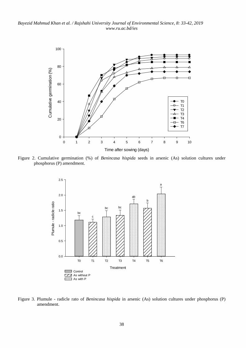
Bayezid Mahmud Khan et al. / Rajshahi University Journal of Environmental Science, 8: 33-42, 2019 www.ru.ac.bd/ies
38
Time after sowing (days)
0 1 2 3 4 5 6 7 8 9 10
Cum
ulat
ive
germ
inat
ion
(%)
0
20
40
60
80
100
T0 T1 T2 T3 T4 T6 T7
Figure 2. Cumulative germination (%) of Benincasa hispida seeds in arsenic (As) solution cultures under
phosphorus (P) amendment.
Treatment
T0 T1 T2 T3 T4 T5 T6
Plum
ule -
radi
cle ra
tio
0.0
0.5
1.0
1.5
2.0
2.5
ControlAs without PAs with P
a
abb
bcbcbc
c
Figure 3. Plumule - radicle rato of Benincasa hispida in arsenic (As) solution cultures under phosphorus (P)
amendment.
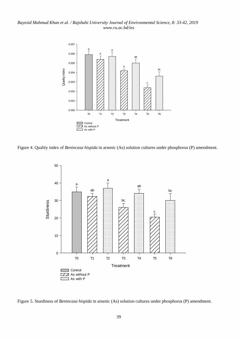
Bayezid Mahmud Khan et al. / Rajshahi University Journal of Environmental Science, 8: 33-42, 2019 www.ru.ac.bd/ies
39
Treatment
T0 T1 T2 T3 T4 T5 T6
Qua
lity
inde
x
0.000
0.001
0.002
0.003
0.004
0.005
0.006
0.007
ControlAs without PAs with P
a
aa
ab
bbc
c
Figure 4. Quality index of Benincasa hispida in arsenic (As) solution cultures under phosphorus (P) amendment.
Treatment
T0 T1 T2 T3 T4 T5 T6
Stu
rdin
ess
0
10
20
30
40
50
ControlAs without PAs with P
aa
abab
bc
bc
c
Figure 5. Sturdiness of Benincasa hispida in arsenic (As) solution cultures under phosphorus (P) amendment.
Bayezid Mahmud Khan et al. / Rajshahi University Journal of Environmental Science, 8: 33-42, 2019 www.ru.ac.bd/ies
40
4. Discussion
Accumulation of As mainly occurs in the root system in plants, and in the aboveground organs to a lesser degree. Such accumulation reduces crop productivity through physiological changes in plants (Stoeva et al., 2005; Leimu and Fischer, 2008; Khan et al., 2013; Meharg et al., 2014; Khan et al., 2018). Arsenic interrupts the biochemical function of cells and severely impedes different plant metabolic processes including transpiration, respiration, photosynthesis etc., by reacting with proteins and enzymes which culminates in stunted plant growth (Meharg and Hartley-Whitaker, 2002). Plants must take up sufficient amount of P to balance excessive As for the alleviation of As toxicity. The plants react to As exposure by increasing P accumulation (Burlo et al., 1999; Leimu and Fischer, 2008; Khan et al., 2013).
This study found that, As solution reduces the rate of seed germination, seedling growth and biomass production of seedling of B. hispida to varying magnitudes based on the level of As concentrations (2ppm, 5 ppm and 10 ppm). However, addition of P (10 ppm) in As solution cultures (2 ppm, 5 ppm and 10 ppm respectively) off setted the harms significantly in comparison to corresponding P-free As solutions. Lou-Hing et al., (2011) also reported that phosphate protects a rice variety- Bala from As toxicity at a lower concentration (13.3 µM) of As in the solution culture. Since As is a phosphate analogue, phosphate transporters transports As which results in competition between P and As for uptake at the level of membrane transport. Accordingly, P is expected to reduce arsenate influx resulting ultimately into an observed increase in arsenate tolerance under phosphate addition (Ullrich-Eberius et al., 1989; Meharg and Macnair, 1990; Khan et al., 2013; Meharg et al., 2014). Studies, especially in hydroponic environments, have demonstrated that non-resistant plants can be made more resistant to arsenate by raising their P status, as the P is taken more effectively compared to arsenate (Meharg and Macnair, 1992b; Lee et al., 2003; Khan et al., 2013). Increasing cytoplasmic phosphate concentration in wheat also demonstrated the role of phosphate against As toxicity (Meharg, 1994). Higher phosphate concentration plays an important role to down-regulation of the arsenate-phosphate plasma membrane transporter and competes with arsenate for biochemical processes where arsenate substitutes for phosphate (Pigna et al., 2009).
5. Conclusion Presence of As reduced the rate of seed germination, seedling growth and biomass production of B. hispida. The addition of P in As solution enhanced the performance of B. hispida seeds and seedlings. Hence, application of P can be recommended to reduce the negative effects of As on B. hispida growth in the laboratory. This similar approach might also be applicable in the field.
References
Abdul-Baki A and Anderson JD. 1973. Vigor determination in Soybean seed by multiple criteria. Crop Science, 13: 630-633.
Adriano DC. 2001. Trace elements in terrestrial environments: Biogeochemistry, bioavailability and risks of metals. Springer, New York.
Babst-Kostecka AA, Waldmann P, Frerot H and Vollenweider P. 2016. Plant adaptation to metal polluted environments- physiological, morphological, and evolutionary insights from Biscutella laevigata. Environmental and Experimental Botany, 127: 1-13.
Bimakr M, Rahman RA, Ganjloo A, Taip FS, Adzahan NM and Sarker MZI. 2016. Characterization of Valuable Compounds from Winter Melon (Benincasa hispida (Thunb.) Cogn.) Seeds Using Supercritical Carbon Dioxide Extraction Combined with Pressure Swing Technique. Food and Bioprocess Technology, 9(3): 396-406.
Bonner FT. 1987. Importance of seed size in germination and seedling growth. In: (Kamra SK and Aylin RD) forest seed problems in Africa, (eds), : 53-61.
Burlo F, Guijarro I, Barrachina AAC and Vlaero D. 1999. Arsenic species: effects on uptake and accumulation by tomato plants. Journal of Agricultural and Food Chemistry, 47: 1247-1253.
Carbonell-Barrachina AA, Burlo F, Burgos-Hernandez A, Lopez E and Mataix J. 1997. The influence of arsenite concentration on arsenic accumulation in tomato and bean plants. Scientia Horticulturae, 71: 167-176.
Bayezid Mahmud Khan et al. / Rajshahi University Journal of Environmental Science, 8: 33-42, 2019 www.ru.ac.bd/ies
41
Chaturvedi I. 2006. Effects of arsenic concentrations and forms on growth and arsenic uptake and accumulation by Indian Mustard (Brassica juncea L.) genotypes. Journal of Central European Agriculture, 7(1): 31-40.
Dickson A, Leaf AL and Hosner JF. 1960. Quality appraisal of white spruce and white pine seedling stock in nurseries. Forestry Chronicle, 36: 10-13.
Fitz WJ and Wenzel WW. 2002. Arsenic transformations in the soil-rhizosphere-plant system: fundamentals and potential application to phytoremediation. Journal of Biotechnology, 99(3): 259-278.
Guevara-Garcia AA, Lara FP, Juarez LK and Herrera-Estrella LR. 2017. Heavy metal adaptation. eLS, 1-9.
Hatchell GE. 1985. Proceedings of the 3rd Biological Southern Research Conference. Shoulders E (ed) Atlanta, Georgia, : 395-402.
Hettick BE. 2016. Arsenic in muskmelon (Cucumis melo) plants and wine in West Texas. https://ttu-ir.tdl.org/ttu-ir/handle/2346/68091 [accessed 28.10. 2017].
Hoagland DR and Arnon DI. 1950. The water culture method for growing plant without soil. California Agricultural Experiment Station Circular, 347: 1-32.
Khan BM, Afrin AH and Hossain MM. 2018. Effects of phosphorus on germination and seedling growth of Cucumis sativus L. in arsenic solution culture. International Journal of Rural Development, Environment and Health Research, 2(1):48-55.
Khan BM, Deacon C, Meharg C, Norton G, Johnson D and Meharg AA. 2013. A balanced polymorphism in biomass resource allocation controlled by phosphate in grasses screened through arsenate tolerance. Environmental and Experimental Botany, 96: 43-51.
Lee DA, Chen A and Schroeder JI. 2003. Ars1, an Arabidopsis mutant exhibiting increased tolerance to arsenate and increased phosphate uptake. The Plant Journal, 35: 637- 646.
Leimu R and Fischer M. 2008. A meta-analysis of local adaptation in plants. PLoS ONE, 3(12): e4010. doi:10.1371/journal.pone.0004010.
Lou-Hing D, Zhang B, Price AH and Meharg AA. 2011. Effects of phosphate on arsenate and arsenite sensitivity in two rice (Oryza sativa L.) cultivars of different sensitivity. Environmental and Experimental Botany, 72: 47-52.
Marschner H. 1995. Mineral nutrition of higher plants. 2nd ed. Academic press, Inc., London.
Meharg AA. 1994. Ecological impact of major industrial-chemical accident. Reviews on Environmental Contamination and Toxicology, 138: 21- 48.
Meharg AA and Hartley-Whitaker J. 2002. Arsenic uptake and metabolism in arsenic resistant and nonresistant plant species. New Phytologist, 154(1): 29-43.
Meharg AA and Macnair MR. 1990. An altered phosphate uptake system in arsenate tolerant Holcus lanatus L. New Phytologist, 116: 29-35.
Meharg AA and Macnair MR. 1992a. Suppression of the high affinity phosphate uptake system: a mechanism of arsenate tolerance in Holcus lanatus L. Journal of Experimental Bototany, 43: 519-524.
Meharg AA and Macnair M.R. 1992b. Genetic correlation between arsenate tolerance and the rate of arsenate and phosphate uptake in Holcus lanatus L. Heredity, 69: 336-341.
Meharg AA and Rahman MA. 2003. Arsenic contamination in Bangladesh paddy field soils: implication for rice contribution to arsenic consumption. Environmental Science and Technology, 37: 229-234.
Meharg C, Khan B, Norton G, Deacon C, Johnson D, Reinhardt R, Huettel B and Meharg AA. 2014. Trait directed de novo population transcriptome dissects genetic regulation of a balanced polymorphism in phosphorus nutrition/arsenate tolerance in a wild grass Holcus lanatus L. New Phytologist, 201:144-154.
Bayezid Mahmud Khan et al. / Rajshahi University Journal of Environmental Science, 8: 33-42, 2019 www.ru.ac.bd/ies
42
Mishra BK, Dubey CS, Shukla DP, Bhattacharya P and Usham AL. 2014. Concentration of arsenic by selected vegetables cultivated in the Yamuna flood plains (YFP) of Delhi, India. Environmental Earth Sciences, 72(9): 3281-3291.
Peryea FJ. 1998. Phosphate starter fertilizer temporarily enhances soil arsenic uptake by apple trees grown under field conditions. HortScience, 33: 826-829.
Pigna M, Cozzalino V, Violante A and Meharg AA. 2009. Influence of phosphate on the arsenic uptake by wheat (Triticum durum L.) irrigated with arsenic solutions at three different concentrations. Water, Air, and Soil Pollution, 197: 371-380.
Raghothama KG. 1999. Phosphate acquisition. Annual Review of Plant Physiology and Plant Molecular Biology, 50: 665-693.
Rayees B, Dorcus M and Chitra S. 2013. Nutritional composition and oil fatty acids of Indian winter melon Benincasa hispida (Thunb.) seeds. International Food Research Journal, 20(3): 1151-1155.
Sanal F, Şeren G and Guuner U. 2014. Effects of arsenate and arsenite on germination and some physiological attributes of barley (Hordeum vulgare L.). Bulletin of Environmental Contamination and Toxicology, 92(4): 483-489.
Singh M, Kumar J, Singh S, Singh VP, Prasad SM and Singh MPVVB. 2015. Adaptation strategies of plants against heavy metal toxicity: A short review. Biochemistry & Pharmacology, 4: 161.
Stoeva N, Berova MA and Zlatev Z. 2005. Effect of arsenic on some physiological parameters in bean plants. Biologia Plantarum, 49: 293-296.
Sultana S, Rashid MH and Huq SMI. 2015. Arsenic accumulation in crops in relation to their water requirement. Bangladesh Journal of Scientific Research, 28(2): 171-180.
Ullrich-Eberius CI, Sanz A and Novacky AJ. 1989. Evaluation of arsenate-and vanadate-associated changes of electrical membrane potential and phosphate transport in Lemna gibba G1. Journal of Experimental Botany, 40(210): 119-128.
Md. Abul Kalam Azad et al. / Rajshahi University Journal of Environmental Science, 8: 43-50, 2019 www.ru.ac.bd/ies
Assessing the Potentiality of Five Medicinal Plant Extracts to Control the Thrips (Scirtothrips bispinosus) of Tea Garden
Md. Abul Kalam Azad1∗, Iftekhar Ahmad1 and Moinuddin Ahmed2
1Department of Food Engineering & Tea Technology, Shahjalal University of Science & Technology, Sylhet-3114,
Bangladesh 2Former Director, Bangladesh Tea Research Institute, Srimangal-3210, Moulvibazar, Bangladesh
Abstract
Several pests including 1034 species of arthropods and 82 species of nematodes are the major pests which attack the tea plants globally. Among them, 25 species of insects, 4 species of mites and 10 species of nematodes are recorded from Bangladesh. In the advent for the search of potentiality of different medicinally important plants to control thrips of tea leaves, this experiment was carried out at lab as well as tea field. Five medicinal plants viz. Monochoria vaginalis, Cassia alata, Nerium odoratum, Annona squamosa and Mikania cordata were used with 50% alcohol extraction in different concentration. Mortality time was counted to quantify the efficiency and potentiality of different plants extracts on thrips named Scirtothrips bispinosusin the field.The result of one-way ANOVA and post hoc analysis reveals that Monochoria vaginalis and Nerium odoratum have the most potential to control the attack of Scirtothrips bispinosus based on time and extract concentration. The Omnibus test reveals that the different concentrations of plant extract have significant effect on the number of mortalities of thrips. The number of deaths of the thrips was found as 5 times higher for 5% concentration than 1% concentration of extract. The death of thrips potentiality was found to decreased with the decreasing of concentrations.
Keywords: Extracts; Medicinal Plant; Tea; Thrips; Potentiality
1. Introduction
In the recent decades, search for pest control products from plants continues to grow, but not always with clear outcomes and benefits (Isman and Grieneisen, 2013). However, there are many plant species with known pesticidal properties where many is already known about their chemistry and efficacy under laboratory conditions (Stevenson et al., 2017). Isman (2017) has argued that increasing use of natural pesticides needs research directed at the practical application of such products under complex agro-ecological conditions, particularly understanding how different pesticidal plant species perform when applied to different crops under different growing conditions. Using unprocessed plant extracts for pest control has several advantages in terms of preventing the development of insecticide resistance due to the usual presence of several bio-active compounds, their low persistence in the environment and their generally low cost of use, particularly for smallholder farmers with limited income (Angioni et al, 2005; Caboni et al, 2006; Isman 2008). Consumers and policy makers are demanding reduced synthetic inputs in food production, and practices that support agro-ecological intensification and pesticidal plant products may be well suited to this vision (Grzywacz et al., 2014; Sola et al., 2014; Pavela 2016).
Tea is one of the most consumed non-alcoholic as well as medicinal beverages in the world. At present, more than 58 countries around the world produce tea, while Bangladesh is now ranked 10th position amongst the tea growing countries. But tea plants are subjected to the attack of insects, mites and nematode pests (Paul et al, 2017). Mamun et al., (2016) reported that about 15% of tea production could be lost per year by various pests particularly insects, mites and nematodes if adequate control measures are not taken in Bangladesh. So far, 25 insect, four mites and 10 nematode species of tea related species had been recorded in Bangladesh (Sana 1989; Ahmed, 2005). Due to climate change, pest infestation is increasing as well as pest status is changing (Noori et al., 2016). Besides, deforestation is resulting in the migration of forest pest to tea ecosystem (Antony et al., 2012). Natural bio-control agents play an important role to regulate the pest population in tea ecosystem. Existence of more than one hundred species of indigenous natural bio-control agents of tea pests including predators, parasites and parasitoids were recorded from the tea ecosystem (Borthakur et al., 2010).
∗ Corresponding author’s e-mail: [email protected]
Md. Abul Kalam Azad et al. / Rajshahi University Journal of Environmental Science, 8: 43-50, 2019 www.ru.ac.bd/ies
44
The increasing awareness of negative effects of synthetic pesticide on human and animal health and the agro-ecosystem, research efforts on alternative and more environmentally friendly methods of controlling pests and diseases have proliferated (Zhou et al., 2019, Hagstrum and Athanassiou, 2019). Usage of extract from plants containing natural anti-pest compounds for pest control is considered to be one of the desirable methods for plant protection in agriculture (Kim et al., 2003). In recent past, several plant species had been screened for anti-pest activity and extracts/purified compounds from these plants were found to have a broad spectrum of anti-pest activity (Grayer and Harborne, 1994). Considering the above evidences, the present study was undertaken to find out most potential plant extract against Scirtothrips bispinosus (tea leaf’s thrips). It is expected that the output of the study could be helpful to provide information regarding plant-insect interaction and to predict suitable techniques for controlling tea pests naturally.
2. Materials and Methods
Tea leaves were used as the basic elements for this study which were infected by thrips. These infected leaves were collected from Habibnagar Tea Estate and Khan Tea Estate in Sylhet, and Baraoora Tea Estate in Moulvibazar district of Bangladesh. Climate of this region is considered sub-tropical monsoon with three distinct seasons: pre-monsoon season (February to April), monsoon season (May to August) and winter season (September to January). It was observed that about 1400 mm of annual rainfall is a critical limit and the monthly mean temperature is between 18.33°C to 29.44°C seem unfavorable for tea production in Bangladesh (Ahmed 2005 and Sana, 1989).
In this study, five plants extracts were used. The plants were Monochoria vaginalis (Bhat Meteka/ Panee Kachu), Cassia alata (Dadmurdan), Nerium odoratum (Karabi/Raktakarabi), Annona squamosa (Ata/Ata Phol) and Mikania cordata (Refusilata/Jarmanilata). The leaf of five plants were collected and dried in the sun. Fully dried leaf is grinded into fine powder and then placed into 50% alcohol as solvent. The solvent to sample ratio were 4:1. The conical were screw caped and placed in a shaker at room temperature for 24 h at 100 rpm. After 24 h, the extracts were filtered using a muslin cloth and then re-filtered using Whatman filter paper No.1. The extracts were labeled accordingly and preserved in the refrigerator at 4°C, till further work. The collection of thrips affected plants were repeated for three times. For each replication, four densities i.e., 1%, 5%, 10% and 15% concentration of extract were used to observe the number of mortalities of thrips out of total 12 thrips for each plant. The plant leaves were used to get the essence of plants using 50% alcohol and used it on the leaves in different concentrations. At the same time different duration of mortality of thrips were also observed. The experiment was designed to find out the potentiality of plant extracts for the mortality of thrips based on concentration and duration of time, and also find out the impact of different concentrations of extract on the mortality of thrips among the extracted plants. The plants were collected randomly from different places of Bangladesh. A total of 60 samples (thrips affected leaves), 12 for each plant were used in this study. Using in vitro method, 5 ml essence of plants were used for each sample. The laboratory work was carried out in the Department of Food Engineering and Tea Technology of Shahjalal University of Science and Technology, Sylhet, Bangladesh during March, 2019 to August, 2019.
Data analysis was carried out using analysis of variance (ANOVA). One-way ANOVA test is a widely used parametric test that is used to determine whether more than two groups have the same means or not (Osteragova and Ostertag, 2013). In this experimental study, ANOVA was used to find out whether there has significance difference in the average mortality of thrips among the five type of plants for the same concentration. For significance difference in the mortality of thrips for different plants, the Post hoc tests were applied to find out the significantly different pairs of plants extracts. To find out the impact of different concentration on the mortality of thrips, a Poisson regression model was applied. Poisson regression model was applied here because of the nature of the dependent variable, the number of mortalities of thrips which follows approximately a Poisson distribution. However, the Poisson loglinear regression model for the expected number of the occurrence of deaths of the thrips (µ) is: log𝑒 𝜇 = 𝛽0 + 𝛽1𝑋
Where, µ is the number of mortalities of thrips and X is the densities of the concentration (categorical type). Because of the small number of replicates and slight violation of equi-dispersion assumption having under-dispersion among samples, the confidence intervals were found to be more compact which was not major concern
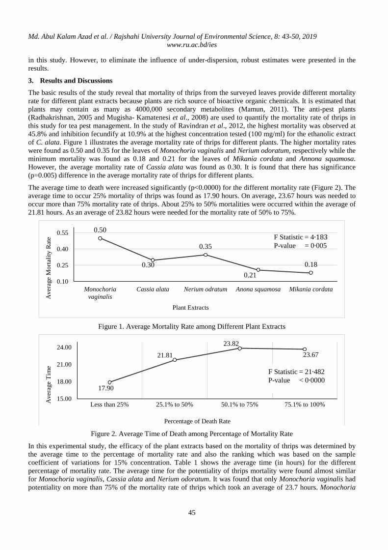
Md. Abul Kalam Azad et al. / Rajshahi University Journal of Environmental Science, 8: 43-50, 2019 www.ru.ac.bd/ies
45
in this study. However, to eliminate the influence of under-dispersion, robust estimates were presented in the results.
3. Results and Discussions
The basic results of the study reveal that mortality of thrips from the surveyed leaves provide different mortality rate for different plant extracts because plants are rich source of bioactive organic chemicals. It is estimated that plants may contain as many as 4000,000 secondary metabolites (Mamun, 2011). The anti-pest plants (Radhakrishnan, 2005 and Mugisha- Kamatenesi et al., 2008) are used to quantify the mortality rate of thrips in this study for tea pest management. In the study of Ravindran et al., 2012, the highest mortality was observed at 45.8% and inhibition fecundify at 10.9% at the highest concentration tested (100 mg/ml) for the ethanolic extract of C. alata. Figure 1 illustrates the average mortality rate of thrips for different plants. The higher mortality rates were found as 0.50 and 0.35 for the leaves of Monochoria vaginalis and Nerium odoratum, respectively while the minimum mortality was found as 0.18 and 0.21 for the leaves of Mikania cordata and Annona squamosa. However, the average mortality rate of Cassia alata was found as 0.30. It is found that there has significance (p=0.005) difference in the average mortality rate of thrips for different plants.
The average time to death were increased significantly (p<0.0000) for the different mortality rate (Figure 2). The average time to occur 25% mortality of thrips was found as 17.90 hours. On average, 23.67 hours was needed to occur more than 75% mortality rate of thrips. About 25% to 50% mortalities were occurred within the average of 21.81 hours. As an average of 23.82 hours were needed for the mortality rate of 50% to 75%.
Figure 1. Average Mortality Rate among Different Plant Extracts
Figure 2. Average Time of Death among Percentage of Mortality Rate
In this experimental study, the efficacy of the plant extracts based on the mortality of thrips was determined by the average time to the percentage of mortality rate and also the ranking which was based on the sample coefficient of variations for 15% concentration. Table 1 shows the average time (in hours) for the different percentage of mortality rate. The average time for the potentiality of thrips mortality were found almost similar for Monochoria vaginalis, Cassia alata and Nerium odoratum. It was found that only Monochoria vaginalis had potentiality on more than 75% of the mortality rate of thrips which took an average of 23.7 hours. Monochoria
0.50
0.30
0.35
0.21 0.18
0.10
0.25
0.40
0.55
Monochoriavaginalis
Cassia alata Nerium odratum Anona squamosa Mikania cordata
Ave
rage
Mor
talit
y R
ate
Plant Extracts
F Statistic = 4∙183 P-value = 0∙005
17.90
21.81
23.82 23.67
15.00
18.00
21.00
24.00
Less than 25% 25.1% to 50% 50.1% to 75% 75.1% to 100%Ave
rage
Tim
e
Percentage of Death Rate
F Statistic = 21∙482 P-value < 0∙0000
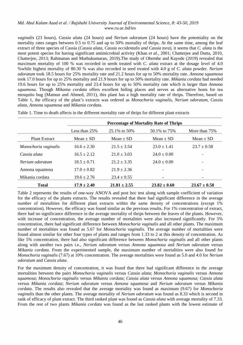
Md. Abul Kalam Azad et al. / Rajshahi University Journal of Environmental Science, 8: 43-50, 2019 www.ru.ac.bd/ies
46
vaginalis (23 hours), Cassia alata (24 hours) and Nerium odoratum (24 hours) have the potentiality on the mortality rates ranges between 0.5 to 0.75 and up to 50% mortality of thrips. At the same time, among the leaf extract of three species of Cassia (Cassia alata, Cassia occidentalis and Cassia tora), it seems that C. alata is the most potent species for having significant antimicrobial activity (Khan et al., 2001; Chatterjee and Dutta, 2010, Chatterjee, 2013; Rahmanan and Muthukumaran, 2019).The study of Obembe and Kayode (2019) revealed that maximum mortality of 100 % was recorded in seeds treated with C. alata extract at the dosage level of 4.0 %while highest mortality of 80.30 % was also recorded in seed treated with 4.0 g of C. alata powder. Nerium odoratum took 18.5 hours for 25% mortality rate and 21.2 hours for up to 50% mortality rate. Annona squamosa took 17.0 hours for up to 25% mortality and 21.9 hours for up to 50% mortality rate. Mikania cordata had needed 19.6 hours for up to 25% mortality and 23.4 hours for up to 50% mortality rate which is larger than Annona squamosa. Though Mikania cordata offers excellent hiding places and serves as alternative hosts for tea mosquito bug (Mamun and Ahmed, 2011), this plant has a high mortality rate of thrips. Therefore, based on Table 1, the efficacy of the plant’s extracts was ordered as Monochoria vaginalis, Nerium odoratum, Cassia alata, Annona squamosa and Mikania cordata.
Table 1. Time to death affects in the different mortality rate of thrips for different plant extracts
Percentage of Mortality Rate of Thrips
Less than 25% 25.1% to 50% 50.1% to 75% More than 75%
Plant Extract Mean ± SD Mean ± SD Mean ± SD Mean ± SD
Monochoria vaginalis 16.6 ± 2.30 21.5 ± 3.54 23.0 ± 1.41 23.7 ± 0.58
Cassia alata 16.5 ± 2.12 21.0 ± 3.03 24.0 ± 0.00 -
Nerium odoratum 18.5 ± 0.71 21.2 ± 3.35 24.0 ± 0.00 -
Annona squamosa 17.0 ± 0.82 21.9 ± 2.36 - -
Mikania cordata 19.6 ± 2.76 23.4 ± 0.55 - -
Total 17.9 ± 2.40 21.81 ± 2.55 23.82 ± 0.60 23.67 ± 0.58
Table 2 represents the results of one-way ANOVA and post hoc test along with sample coefficient of variation for the efficacy of the plants extracts. The results revealed that there had significant difference in the average number of mortalities for different plant extracts within the same density of concentrations (except 1% concentration). However, the efficacy was found similar as the previous results. For 1% concentration of extract, there had no significance difference in the average mortality of thrips between the leaves of the plants. However, with increase of concentration, the average number of mortalities were also increased significantly. For 5% concentration, there had significant difference between Monochoria vaginalis and all other plants. The maximum number of mortalities was found as 5.67 for Monochoria vaginalis. The average number of mortalities were found almost similar for other four types of plants and ranges from 1.33 to 2 at this density of concentration. As like 5% concentration, there had also significant difference between Monochoria vaginalis and all other plants along with another two pairs i.e., Nerium odoratum versus Annona squamosa and Nerium odoratum versus Mikania cordata. From the experimented sample, the maximum number of mortalities were also found for Monochoria vaginalis (7.67) at 10% concentration. The average mortalities were found as 5.0 and 4.0 for Nerium odoratum and Cassia alata.
For the maximum density of concentration, it was found that there had significant difference in the average mortalities between the pairs Monochoria vaginalis versus Cassia alata; Monochoria vaginalis versus Annona squamosa; Monochoria vaginalis versus Mikania cordata; Cassia alata versus Annona squamosa; Cassia alata versus Mikania cordata; Nerium odoratum versus Annona squamosa and Nerium odoratum versus Mikania cordata. The results also revealed that the average mortality was found as maximum (9.67) for Monochoria vaginalis than the other plants. The average mortality of Nerium odoratum was found as 8.33 which is second in rank of efficacy of plant extract. The third ranked plant was found as Cassia alata with average mortality of 7.33. From the rest of two plants Mikania cordata was found as the last ranked plants with the lowest estimate of
Md. Abul Kalam Azad et al. / Rajshahi University Journal of Environmental Science, 8: 43-50, 2019 www.ru.ac.bd/ies
47
average mortality (4.33). Therefore, at 10% concentration, the rank was found by following Monochoria vaginalis, Nerium odoratum, Cassia alata, Annona squamosa and Mikania cordata respectively that is considerable for other medicinal plants like Ipomoea crassicaulis, Lantana camara, Ipomoea hederaceaa, Glycosmis arborea, and Justicia gendarussa (Azad et al., 2020).
Table 2. Number of mortalities of thrips in different concentration of plant extract for different plant extracts
Mortality at Different Concentration of Plant extract
1% 5% 10% 15%
Plant Extracts Mean ± SD Mean ± SD Mean ± SD Mean ± SD CV Ranking
Monochoria vaginalis
1.00a ± 0.00 5.67a ± 0.58 7.67a ± 0.58 9.67a ± 0.58 5.99 1
Cassia alata 1.00a ± 0.00 2.00b ± 0.00 4.00bc ± 0.00 7.33b ± 0.58 7.91 3
Nerium odoratum 1.33a ± 0.58 2.00b ± 0.00 5.00b ± 1.00 8.33ab ± 0.58 6.96 2
Annona squamosa 0.33a ± 0.58 1.33b ± 0.58 3.00c ± 0.00 5.33c ± 0.58 10.88 4
Mikania cordata 0.33a ± 0.58 1.33b ± 0.58 2.67c ± 0.58 4.33c ± 0.58 13.39 5
Total 0.80 ± 0.56 2.47 ± 1.73 4.47 ± 1.92 7.00 ± 2.07 - -
Means within column followed by the same letters are not significantly different based on Tukey’s Post Hoc (Liu,et al. 2015) test at p = 0.05.
Poisson regression was used in Table 3 to determine the significant impact of different densities of concentration on the mortality of thrips for the plant extracts. The table shows the parameter estimates of the Poisson regression model along with Wald 95% confidence interval. The Omnibus test revealed that the different concentrations of alcohol have significant effect on the number of mortalities of thrips. The number of deaths of the thrips was found almost three times higher (Exp(1.126)=3.083) for 5% concentration than the 1% concentration of extract. The deaths were found as almost 5.5 times higher (Exp(1.72)=5.583) in 10% concentration as compared to 1% concentration. However, for further increase of the centration (15%), the number of deaths were increases as 8.75 times (Exp(2.169)=8.75) than the lowest densities of concentration (1%).
Table 3. Estimates of Poisson Regression Model along with 95% Confidence Interval
Parameters Estimates, β 95% CI of β Exp(β) 95% CI of Exp(β)
Intercept -0.223 [-0.566, 1.119] 0.800 [0.568, 1.127]
1% Concentration (Reference group)
5% Concentration 1.126 [0.642, 1.610] 3.083 [1.900, 5.004]
10% Concentration 1.720 [1.318, 2.122] 5.583 [3.735, 8.346]
15% Concentration 2.169 [1.797, 2.541] 8.750 [6.003, 12.691]
Omnibus test result: Likelihood Ratio Chi-square = 94.36, P-value <0.0000
4. Conclusion
Five types of medicinal plant extracts were used in this study to find out the potentiality of extracts on tea thrips at different concentrations. It was found that the plant extracts had potential to control the tea thrips (on mortality) based on time and concentration. Only Monochoria vaginalis had potentiality on more than 75% of the mortality rate of thrips which took an average 23.7 hours. Result shows that Monochoria vaginalis had the minimum CV value (5.99) than Nerium odoratum, Cassia alata, Annona squamosa and Mikania cordata. So, Monochoria vaginalis extracts was found to be most potential plant depending on the time of death affect among the five medicinal plants used in this study.
Md. Abul Kalam Azad et al. / Rajshahi University Journal of Environmental Science, 8: 43-50, 2019 www.ru.ac.bd/ies
48
References
Ahmed M. 2005. Tea Pest Management. Evergreen Printing and Packaging. Dhaka, Bangladesh, pp. 118.
Azad MAK, Ahmad A and Mainuddin A. 2020. Application of plant extracts for pest management in tea: a study on tea leaf’s thrips, Scirtothripsbispinosus. Journal of Bio-Sci, 28: 87-93.
Angioni A, Dedola F, Minelli EV, Barra A, Cabras P, and Caboni P. 2005. Residues and half-life times of pyrethrins on peaches after field treatments. Journal of Agriculture amd Food Chemistry, 53: 4059–4063.
Antony B, Sinu PA and Rahman A. 2012. Looper caterpillar invasion in North-East Indian tea agro-ecosystem: Change of weather and habitat loss may be possible causes. Journal of Tea Science Research, 2(1): 1-5.
Borthakur M, Rahman A and Sarmah S. 2010. Pest management in tea in North East India. Bul. UPASI Tea Res. Found. 55: 10-18.
Caboni P, Sarais G, Angioni A, Garcia AJ, Lai F, Dedola F. 2006. Residues and persistence of neem formulations on strawberry after field treatment. Journal of Agriculture amd Food Chemistry, 54: 10026–10032.
Chatterjee S, Chatterjee S, Dutta S .2010. A survey on VAM association in three different species of Cassia and determination of antimicrobial property of these phytoextracts. J Med Plants Res, 4: 286-292.
Chatterjee S. 2013. Cassia alata - a useful antimicrobial agent. Med Aromat Plants, 2: e143.
Gadzirayi CT, Mutandwa E, Mwale M, and Chindundu T. 2009. Utilization of Tephrosia vogelii in controlling ticks in dairy cows by small Scale commercial farmers in Zimbabwe. African Journal of Biotechnology, 8: 4134–4136.
Grayer RJ and Harborne JB. 1994. A Survey of antifungal compounds from higher plants, Phytochemistry, 37: 19-42.
Hagstrum DW and Athanassiou CG. 2019. Improving stored product insect pest management: From theory to practice. Insects, 10 (332): 1-7.
Isman MB. 2008. Botanical insecticides: for richer, for poorer. Pest Management Science, 64: 8–11.
Isman MB. 2017. Bridging the gap: moving botanical insecticides from the laboratory to the farm. Industrial Crops and Production,11: 10–14.
Isman MB and Grieneisen ML. 2013. Botanical insecticide research: many publications, limited useful data. Trends Plant Science, 19:140–145.
Khan MR, Kihara M and Omoloso AD. 2001. Antimicrobial activity of Cassia alata. Fitoterapia, 72: 561-564.
Kim Y, Lee S, Yu Y and Han S. 2003. An edible alginate micro-capsulation of entomopathogenic nematode, Steinernemacarocapsae. Korean Journal of Applied Entomopathogenic, 42: 145-152.
Liu S, Li Z, Sui Y, Schaefer DA, Alele PO, Chen JC and Yang X. 2015. Spider foraging strategies dominate pest suppressionin organic tea plantations. Journal of Biological Control, 1-8.
Mamun, MSA. 2011. Prospect of Indigenous Plant Extracts in Tea Pest Management. International Journal of Agricultural Research Innovation and Technology, 1(1&2): 16-23.
Mamun, MSA and Ahmed M. 2011. Integrated pest management in tea: prospects and future strategies in Bangladesh. The Journal of Plant Protection Sciences, 3(2):1-13.
Mamun, MSA, Hoque MM, Ahmed M, Akandha MYH and Paul SK. 2016. Evaluation of some potential miticides against red spider mite infesting tea in Bangladesh. Tea Journal of Bangladesh, 45: 52-64.
Mugisha-Kamatenesi M, Deng AL, OgendoJO, Omolo EO, Mihale MJ, Otim JP,Buyungo and Bet, PK. 2008. Indigenous knowledge of field insect pests and their management around Lake Victoria basin in Uganda. Africa Journal of Environmental Science and Technology, 2(8): 342-348.
Md. Abul Kalam Azad et al. / Rajshahi University Journal of Environmental Science, 8: 43-50, 2019 www.ru.ac.bd/ies
49
Noori MN, Mamun MSA and Ali M. 2016. Impact of climate change on tea production in Bangladesh: A case study on Bilashcherra Experimental Farm. Tea Journal of Bangladesh, 45: 24-34.
Obembe OM and Kayode J. 2019. Evaluation of the insecticidal properties of Cassia alata L. Against cowpea weevil, Callobruchus maculatus Fab.(Coleoptera: Bruchidae). Budapest International Research in Exact Sciences (BirEx) Journal, 1(4): 84-92.
Ostertagova E and Ostertag O. 2013. Methodology and application of one-way ANOVA. American Journal of Mechanical Engineering, 1(7), 256-261.
Paul SK, Ahmed M, Mamun MSA and Alam MJ. 2017. Diversity of insect, mite and nematode species in tea ecosystem of Bangladesh. Journal of Biodiversity Conservation and Bioresources Management, 3(1): 31-44.
Pavela R. 2016. History, presence and perspective of using plant extracts as commercial botanical insecticides and farm products for protection against insects-a review. Agricultural Journal of Plant Protection Science, 52: 229–241.
Radhakrishnan, B. 2005. Indigenouspreparations useful for pest and diseasemanagement. Planters’ Chronicle, 101(4):4-16.
Rahmanan M and Muthukumaran N. 2019. Anti-insect effect of Senna alata L. seed solvent extracts on Spodoptera litura Fab. Journal of Pharmacognosy and Phytochemistry, 2: 401-405.
Ravindran R, Juliet S, Sunil AR, Gopalan K, Kumar A, Nair SN, Amithamol KK, Bandyopadhayay A, Rawat AKS and Ghosh S. 2012. Acaricidal activity of Cassia alata against Rhipicephalus annulatus (Boophilus). Exp Appl Acarol, 56:69–74.
Sana DL. 1989. Tea Science. Ashrafia Boi Ghar, Dhaka, Bangladesh, pp.120-197.
Sola P, Mvumi BM, Ogendo JO, Mponda O, Kamanula JF and Nyirenda SP. 2014. Botanical pesticide production, trade and regulatory mechanisms in sub-Saharan Africa: making a case for plant-based pesticidal products. Food Security, 6: 369–384.
Stevenson PC, Isman MB and Belmain, SR. 2017. Pesticidal plants in Africa: a global vision of new biological control products from local uses. Industrial Crops Production, 110: 2–9.
Zhou Q, Cheng X, Wang S, Liu S and Wei C. 2019. Imidacloprid on the release of C6 green leaf volatiles in tea plants (Camellia sinensis). Scientific Reports, 625: 1-6.

Md. Abul Kalam Azad et al. / Rajshahi University Journal of Environmental Science, 8: 43-50, 2019 www.ru.ac.bd/ies
50
Most. Farida Parvin et al. / Rajshahi University Journal of Environmental Science, 8: 51-58, 2019 www.ru.ac.bd/ies
Some Biological Parameters of Asian Stinging Catfish, Heteropneustes fossilis (Bloch, 1794) (Teleostei: Siluriformes) in the Padma River
Most. Farida Parvin1∗, Akhery Nima2,3, Farzana Akter Rima2 and Md. Yeamin Hossain2
1Institute of Environmental science (IES), University of Rajshahi, Rajshahi-6205, Bangladesh
2Department of Fisheries, Faculty of Agriculture, University of Rajshahi, Rajshahi-6205, Bangladesh 3 Riverine Station, Bangladesh Fisheries Research Institute, Chandpur- 3600, Bangladesh
Abstract
The Stinging catfish, Heteropneustes fossilis (Bloch, 1974) is a commercially important fish species in Asia. The present study reveals life history traits of H. fossilis including population structure, growth pattern (length-weight relationships, LWRs; length-length relationship, LLR), conditions, prey-predator status (relative weight, WR), form factor (a3.0), size at first sexual maturity (Lm) and natural mortality (MW) of H. fossilis from the Padma River, northwestern Bangladesh. A total of 344 individuals of H. fossilis were captured by various types of traditional fishing gears during July 2 0 18 to June 2019 and measured biometric data for each individual. The recorded results showed that the total length was varied from 8.50 to 28.70 cm and Body weight was ranged from 3.12 to 146.55 g. All LWRs were significant (p<0.001), with r2 values ≥ 0.968. The calculated allometric coefficient (b) showed positive allometric growth in combined sexes (b > 3.00). The LLR was significant (p<0.001) with r2 value > 0.995. The a3.0, Lm, and MW were 0.0060, 16.45 cm TL and 0.93 per year for H. fossilis in the Padma River, respectively. These findings would be very effective for further stock assessment and management of this fish in the Padma River and adjoining ecosystems.
Keywords: Growth Pattern; Heteropneustes fossili; Size; Sexual Maturity; Natural Mortality.
1. Introduction
The stinging catfish belongs to the family Heteropneustidae under the order Siluriformes (locally called shing, shinghi) is primarily a fish of ponds, ditches, beels, swamps and marshes but sometimes found in muddy rivers (Jha and Rayamajhi, 2010; Froese and Pouly, 2019). This fish is locally known as Singi in Bangladesh (Talwar and Jhingran, 1991). It is an indigenous species in Asian countries including Bangladesh, India, Nepal, Pakistan, Sri Lanka, Myanmar and Thailand (Talwar and Jhingran, 1991). It is commercially important as a popular food fish. It is caught by small-and large-scale commercial fishers operating in the Padma River with a variety of traditional fishing gears (Craig et al., 2004; Hossain, 2010). The conservation status of this catfish has been categorized as a species of least concern in Bangladesh (IUCN Bangladesh, 2015) and worldwide (IUCN, 2017). Information on population parameters i.e., growth, reproduction, recruitment as well as mortality of fishes is vital to the implementation of sustainable management strategies for their better conservation (Rahman et al., 2012; Hossain et al., 2012a, 2015, 2016). A sum of studies including length-length relationship, length-weight relationships (LWRs) and condition factors (Muhammad et al., 2012; Alam and Ferdaushy, 2015; Das et al., 2015; Hossain et al., 2017; Khan et al., 2012) of this fish species have been conducted, but to the best of authors’ knowledge to date, there is no previous studies on this aspects of H. fossilis from Padma River of Bangladesh. Therefore, the present study was aimed to describe some biological parameters including, population structure, growth pattern, best condition factor, prey-predator status, form factor (a3.0), size at first sexual maturity (Lm) and natural mortality (Mw) of H. fossilis in the Padma River, northwestern part of Bangladesh using a number of specimen with various sizes over the study period of one year.
2. Materials and Methods
2.1. Sampling and Measurement
The present study was carried out in the Padma River in Bangladesh (Charghat: 24°15' N, 88°44' E; and Shaheb Bazaar: 24°20' N, 88°34'), northwestern part of Bangladesh. Samples of H. fossilis were collected occasionally from the fishers’ catch during July 2018 to June 2019. The random sampling method was used for sampling of fish. This fishes typically captured by using different types of traditional fishing gears like, gill net, cast net, ∗ Corresponding author’s e-mail: [email protected]
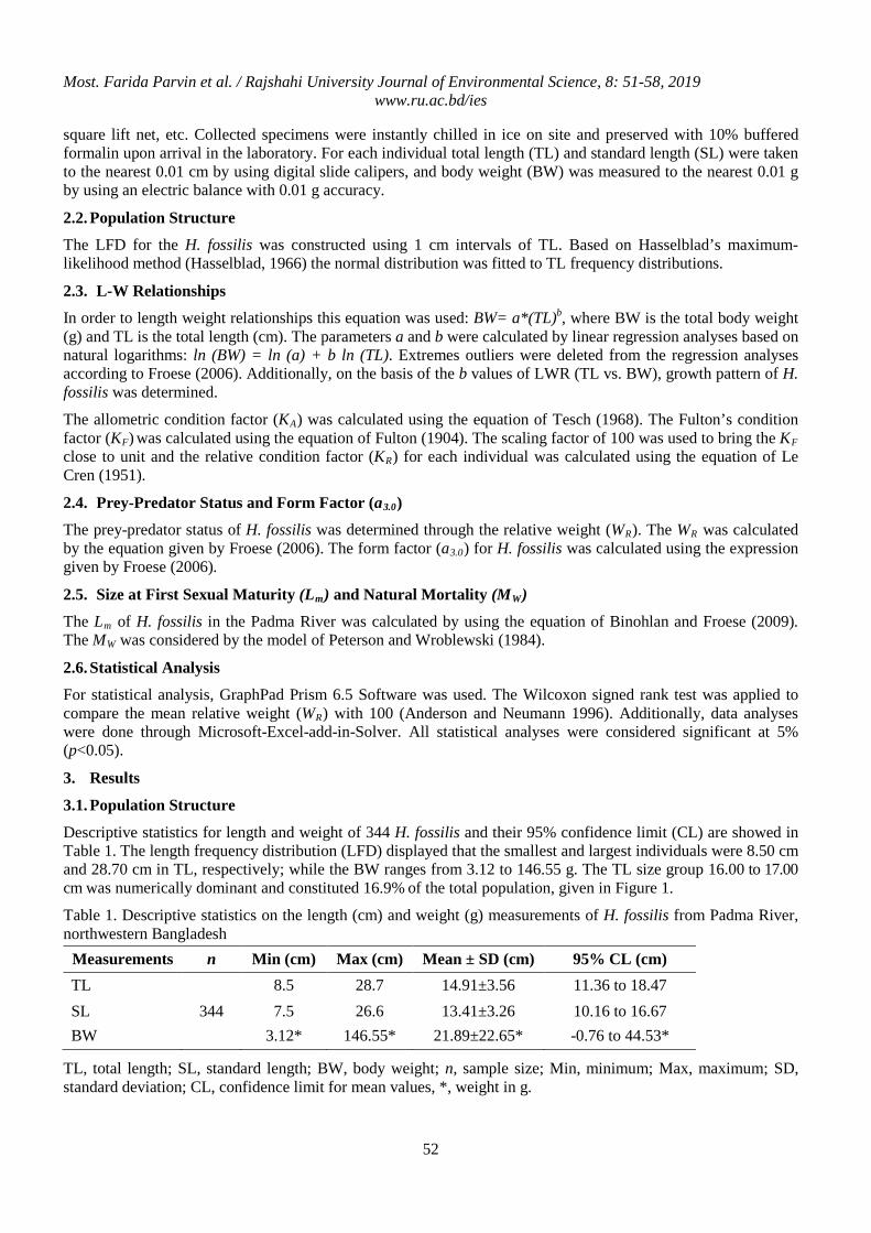
Most. Farida Parvin et al. / Rajshahi University Journal of Environmental Science, 8: 51-58, 2019 www.ru.ac.bd/ies
52
square lift net, etc. Collected specimens were instantly chilled in ice on site and preserved with 10% buffered formalin upon arrival in the laboratory. For each individual total length (TL) and standard length (SL) were taken to the nearest 0.01 cm by using digital slide calipers, and body weight (BW) was measured to the nearest 0.01 g by using an electric balance with 0.01 g accuracy.
2.2. Population Structure
The LFD for the H. fossilis was constructed using 1 cm intervals of TL. Based on Hasselblad’s maximum-likelihood method (Hasselblad, 1966) the normal distribution was fitted to TL frequency distributions.
2.3. L-W Relationships
In order to length weight relationships this equation was used: BW= a*(TL)b, where BW is the total body weight (g) and TL is the total length (cm). The parameters a and b were calculated by linear regression analyses based on natural logarithms: ln (BW) = ln (a) + b ln (TL). Extremes outliers were deleted from the regression analyses according to Froese (2006). Additionally, on the basis of the b values of LWR (TL vs. BW), growth pattern of H. fossilis was determined.
The allometric condition factor (KA) was calculated using the equation of Tesch (1968). The Fulton’s condition factor (KF) was calculated using the equation of Fulton (1904). The scaling factor of 100 was used to bring the KF close to unit and the relative condition factor (KR) for each individual was calculated using the equation of Le Cren (1951).
2.4. Prey-Predator Status and Form Factor (a3.0)
The prey-predator status of H. fossilis was determined through the relative weight (WR). The WR was calculated by the equation given by Froese (2006). The form factor (a3.0) for H. fossilis was calculated using the expression given by Froese (2006).
2.5. Size at First Sexual Maturity (Lm) and Natural Mortality (MW)
The Lm of H. fossilis in the Padma River was calculated by using the equation of Binohlan and Froese (2009). The MW was considered by the model of Peterson and Wroblewski (1984).
2.6. Statistical Analysis
For statistical analysis, GraphPad Prism 6.5 Software was used. The Wilcoxon signed rank test was applied to compare the mean relative weight (WR) with 100 (Anderson and Neumann 1996). Additionally, data analyses were done through Microsoft-Excel-add-in-Solver. All statistical analyses were considered significant at 5% (p<0.05).
3. Results
3.1. Population Structure
Descriptive statistics for length and weight of 344 H. fossilis and their 95% confidence limit (CL) are showed in Table 1. The length frequency distribution (LFD) displayed that the smallest and largest individuals were 8.50 cm and 28.70 cm in TL, respectively; while the BW ranges from 3.12 to 146.55 g. The TL size group 16.00 to 17.00 cm was numerically dominant and constituted 16.9% of the total population, given in Figure 1.
Table 1. Descriptive statistics on the length (cm) and weight (g) measurements of H. fossilis from Padma River, northwestern Bangladesh
Measurements n Min (cm) Max (cm) Mean ± SD (cm) 95% CL (cm) TL 8.5 28.7 14.91±3.56 11.36 to 18.47 SL 344 7.5 26.6 13.41±3.26 10.16 to 16.67 BW 3.12* 146.55* 21.89±22.65* -0.76 to 44.53*
TL, total length; SL, standard length; BW, body weight; n, sample size; Min, minimum; Max, maximum; SD, standard deviation; CL, confidence limit for mean values, *, weight in g.
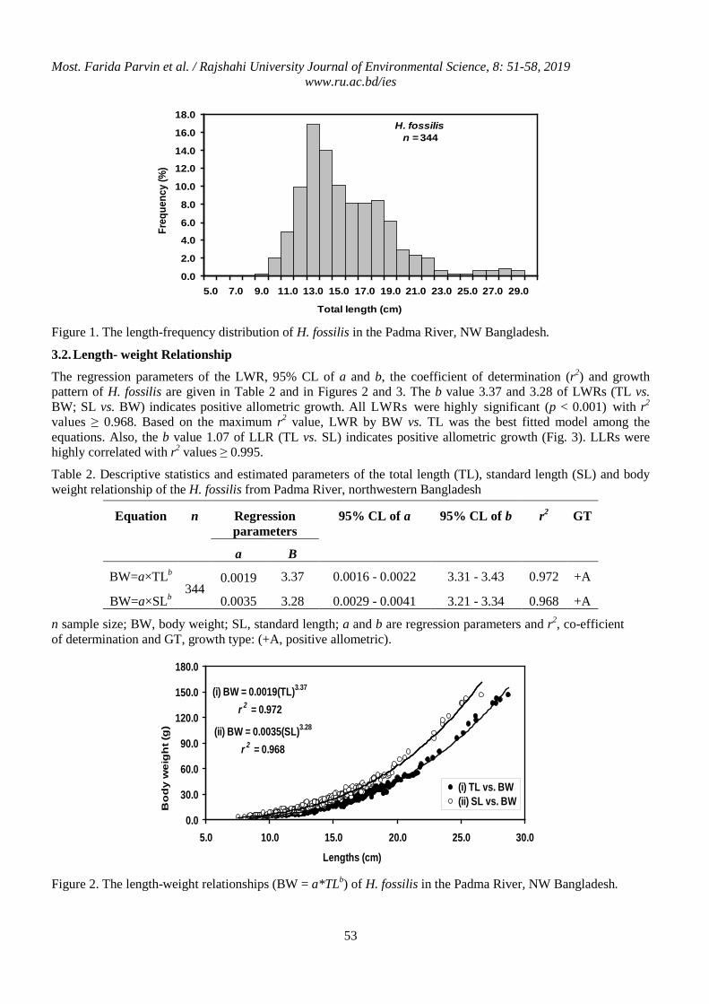
Most. Farida Parvin et al. / Rajshahi University Journal of Environmental Science, 8: 51-58, 2019 www.ru.ac.bd/ies
53
(i) BW = 0.0019(TL)3.37
r 2 = 0.972
(ii) BW = 0.0035(SL)3.28
r 2 = 0.968
0.0
30.0
60.0
90.0
120.0
150.0
180.0
5.0 10.0 15.0 20.0 25.0 30.0Lengths (cm)
Bo
dy
wei
gh
t (g
)
(i) TL vs. BW (ii) SL vs. BW
H. fossilisn = 344
0.0
2.0
4.0
6.0
8.0
10.0
12.0
14.0
16.0
18.0
5.0 7.0 9.0 11.0 13.0 15.0 17.0 19.0 21.0 23.0 25.0 27.0 29.0
Total length (cm)
Freq
uenc
y (%
)
Figure 1. The length-frequency distribution of H. fossilis in the Padma River, NW Bangladesh.
3.2. Length- weight Relationship
The regression parameters of the LWR, 95% CL of a and b, the coefficient of determination (r2) and growth pattern of H. fossilis are given in Table 2 and in Figures 2 and 3. The b value 3.37 and 3.28 of LWRs (TL vs. BW; SL vs. BW) indicates positive allometric growth. All LWRs were highly significant (p < 0.001) with r2 values ≥ 0.968. Based on the maximum r2 value, LWR by BW vs. TL was the best fitted model among the equations. Also, the b value 1.07 of LLR (TL vs. SL) indicates positive allometric growth (Fig. 3). LLRs were highly correlated with r2 values ≥ 0.995.
Table 2. Descriptive statistics and estimated parameters of the total length (TL), standard length (SL) and body weight relationship of the H. fossilis from Padma River, northwestern Bangladesh
Equation n
Regression parameters
95% CL of a 95% CL of b r2 GT
a B BW=a×TLb
344 0.0019 3.37 0.0016 - 0.0022 3.31 - 3.43 0.972 +A
BW=a×SLb 0.0035 3.28 0.0029 - 0.0041 3.21 - 3.34 0.968 +A n sample size; BW, body weight; SL, standard length; a and b are regression parameters and r2, co-efficient of determination and GT, growth type: (+A, positive allometric).
Figure 2. The length-weight relationships (BW = a*TLb) of H. fossilis in the Padma River, NW Bangladesh.
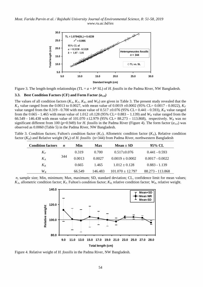
Most. Farida Parvin et al. / Rajshahi University Journal of Environmental Science, 8: 51-58, 2019 www.ru.ac.bd/ies
54
80.0
100.0
120.0
140.0
9.0 11.0 13.0 15.0 17.0 19.0 21.0 23.0 25.0 27.0 28.0
Total length (cm)
Rel
ativ
e w
eigh
t
Mean+SDMean WRMean-SD
Heteropneustes fossilisn = 344
TL = 1.0794(SL) + 0.4239r 2 = 0.995
5.0
10.0
15.0
20.0
25.0
30.0
5.0 10.0 15.0 20.0 25.0 30.0
Standard length (cm)
Tota
l len
gth
(cm
)
TL vs. SL
95% CL of a = 0.3150 - 0.5328b = 1.07 - 1.01
Figure 3. The length-length relationships (TL = a + b* SL) of H. fossilis in the Padma River, NW Bangladesh.
3.3. Best Condition Factors (CF) and Form Factor (a3.0)
The values of all condition factors (KA, KF, KR, and WR) are given in Table 3. The present study revealed that the KA value ranged from the 0.0013 to 0.0027, with mean value of 0.0019 ±0.0002 (95% CL= 0.0017 - 0.0022), KF value ranged from the 0.319 - 0.700 with mean value of 0.517 ±0.076 (95% CL= 0.441 - 0.593), KR value ranged from the 0.665 - 1.465 with mean value of 1.012 ±0.128 (95% CL= 0.883 – 1.139) and WR value ranged from the 66.549 - 146.438 with mean value of 101.070 ±12.979 (95% CL= 88.273 – 113.868), respectively. WR was no significant different from 100 (p=0.949) for H. fossilis in the Padma River (Figure 4). The form factor (a3.0) was observed as 0.0060 (Table 5) in the Padma River, NW Bangladesh.
Table 3. Condition factors; Fulton′s condition factor (KF), Allometric condition factor (KA), Relative condition factor (KR) and Relative weight (WR) of H. fossilis (n=344) from Padma River, northwestern Bangladesh
Condition factors n Min Max Mean ± SD 95% CL KF
344 0.319 0.700 0.517±0.076 0.441 - 0.593
KA 0.0013 0.0027 0.0019 ± 0.0002 0.0017 - 0.0022 KR 0.665 1.465 1.012 ± 0.128 0.883 - 1.139 WR 66.549 146.483 101.070 ± 12.797 88.273 - 113.868
n, sample size; Min, minimum; Max, maximum; SD, standard deviation; CL, confidence limit for mean values; KA, allometric condition factor; KF, Fulton′s condition factor; KR, relative condition factor; WR, relative weight.
Figure 4. Relative weight of H. fossilis in the Padma River, NW Bangladesh.
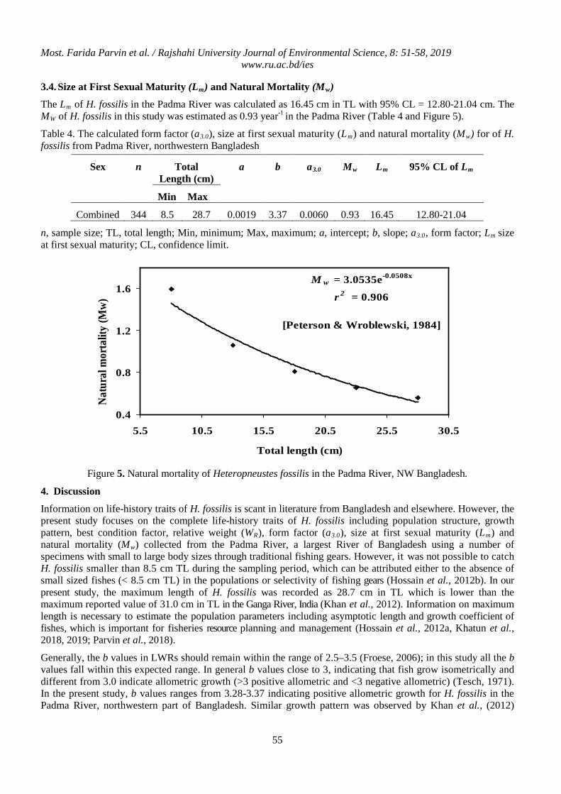
Most. Farida Parvin et al. / Rajshahi University Journal of Environmental Science, 8: 51-58, 2019 www.ru.ac.bd/ies
55
M w = 3.0535e-0.0508x
r 2 = 0.906
[Peterson & Wroblewski, 1984]
0.4
0.8
1.2
1.6
5.5 10.5 15.5 20.5 25.5 30.5
Total length (cm)
Natu
ral m
orta
lity
(Mw)
3.4. Size at First Sexual Maturity (Lm) and Natural Mortality (Mw)
The Lm of H. fossilis in the Padma River was calculated as 16.45 cm in TL with 95% CL = 12.80-21.04 cm. The MW of H. fossilis in this study was estimated as 0.93 year-1 in the Padma River (Table 4 and Figure 5).
Table 4. The calculated form factor (a3.0), size at first sexual maturity (Lm) and natural mortality (Mw) for of H. fossilis from Padma River, northwestern Bangladesh
Sex n Total Length (cm)
a b a3.0 Mw Lm 95% CL of Lm
Min Max Combined 344 8.5 28.7 0.0019 3.37 0.0060 0.93 16.45 12.80-21.04
n, sample size; TL, total length; Min, minimum; Max, maximum; a, intercept; b, slope; a3.0, form factor; Lm size at first sexual maturity; CL, confidence limit.
Figure 5. Natural mortality of Heteropneustes fossilis in the Padma River, NW Bangladesh.
4. Discussion
Information on life-history traits of H. fossilis is scant in literature from Bangladesh and elsewhere. However, the present study focuses on the complete life-history traits of H. fossilis including population structure, growth pattern, best condition factor, relative weight (WR), form factor (a3.0), size at first sexual maturity (Lm) and natural mortality (Mw) collected from the Padma River, a largest River of Bangladesh using a number of specimens with small to large body sizes through traditional fishing gears. However, it was not possible to catch H. fossilis smaller than 8.5 cm TL during the sampling period, which can be attributed either to the absence of small sized fishes (< 8.5 cm TL) in the populations or selectivity of fishing gears (Hossain et al., 2012b). In our present study, the maximum length of H. fossilis was recorded as 28.7 cm in TL which is lower than the maximum reported value of 31.0 cm in TL in the Ganga River, India (Khan et al., 2012). Information on maximum length is necessary to estimate the population parameters including asymptotic length and growth coefficient of fishes, which is important for fisheries resource planning and management (Hossain et al., 2012a, Khatun et al., 2018, 2019; Parvin et al., 2018).
Generally, the b values in LWRs should remain within the range of 2.5–3.5 (Froese, 2006); in this study all the b values fall within this expected range. In general b values close to 3, indicating that fish grow isometrically and different from 3.0 indicate allometric growth (>3 positive allometric and <3 negative allometric) (Tesch, 1971). In the present study, b values ranges from 3.28-3.37 indicating positive allometric growth for H. fossilis in the Padma River, northwestern part of Bangladesh. Similar growth pattern was observed by Khan et al., (2012)
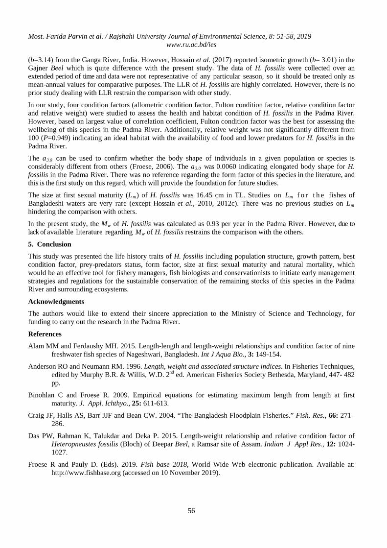
Most. Farida Parvin et al. / Rajshahi University Journal of Environmental Science, 8: 51-58, 2019 www.ru.ac.bd/ies
56
(b=3.14) from the Ganga River, India. However, Hossain et al. (2017) reported isometric growth (b= 3.01) in the Gajner Beel which is quite difference with the present study. The data of H. fossilis were collected over an extended period of time and data were not representative of any particular season, so it should be treated only as mean-annual values for comparative purposes. The LLR of H. fossilis are highly correlated. However, there is no prior study dealing with LLR restrain the comparison with other study.
In our study, four condition factors (allometric condition factor, Fulton condition factor, relative condition factor and relative weight) were studied to assess the health and habitat condition of H. fossilis in the Padma River. However, based on largest value of correlation coefficient, Fulton condition factor was the best for assessing the wellbeing of this species in the Padma River. Additionally, relative weight was not significantly different from 100 (P=0.949) indicating an ideal habitat with the availability of food and lower predators for H. fossilis in the Padma River.
The a3.0 can be used to confirm whether the body shape of individuals in a given population or species is considerably different from others (Froese, 2006). The a3.0 was 0.0060 indicating elongated body shape for H. fossilis in the Padma River. There was no reference regarding the form factor of this species in the literature, and this is the first study on this regard, which will provide the foundation for future studies.
The size at first sexual maturity (Lm) of H. fossilis was 16.45 cm in TL. Studies on Lm f o r t h e fishes of Bangladeshi waters are very rare (except Hossain et al., 2010, 2012c). There was no previous studies on Lm hindering the comparison with others.
In the present study, the Mw of H. fossilis was calculated as 0.93 per year in the Padma River. However, due to lack of available literature regarding Mw of H. fossilis restrains the comparison with the others.
5. Conclusion
This study was presented the life history traits of H. fossilis including population structure, growth pattern, best condition factor, prey-predators status, form factor, size at first sexual maturity and natural mortality, which would be an effective tool for fishery managers, fish biologists and conservationists to initiate early management strategies and regulations for the sustainable conservation of the remaining stocks of this species in the Padma River and surrounding ecosystems.
Acknowledgments
The authors would like to extend their sincere appreciation to the Ministry of Science and Technology, for funding to carry out the research in the Padma River.
References
Alam MM and Ferdaushy MH. 2015. Length-length and length-weight relationships and condition factor of nine freshwater fish species of Nageshwari, Bangladesh. Int J Aqua Bio., 3: 149-154.
Anderson RO and Neumann RM. 1996. Length, weight and associated structure indices. In Fisheries Techniques, edited by Murphy B.R. & Willis, W.D. 2nd ed. American Fisheries Society Bethesda, Maryland, 447- 482 pp.
Binohlan C and Froese R. 2009. Empirical equations for estimating maximum length from length at first maturity. J. Appl. Ichthyo., 25: 611-613.
Craig JF, Halls AS, Barr JJF and Bean CW. 2004. “The Bangladesh Floodplain Fisheries.” Fish. Res., 66: 271–286.
Das PW, Rahman K, Talukdar and Deka P. 2015. Length-weight relationship and relative condition factor of Heteropneustes fossilis (Bloch) of Deepar Beel, a Ramsar site of Assam. Indian J Appl Res., 12: 1024-1027.
Froese R and Pauly D. (Eds). 2019. Fish base 2018, World Wide Web electronic publication. Available at: http://www.fishbase.org (accessed on 10 November 2019).
Most. Farida Parvin et al. / Rajshahi University Journal of Environmental Science, 8: 51-58, 2019 www.ru.ac.bd/ies
57
Froese R, Tsikliras AC and Stergiou KI. 2011. Editorial note on weight-length relations of fishes. Acta Ichthyol Pisc., 41: 261-263.
Froese R. 2006. Cube law, condition factor and weight-length relationships: history, meta-analysis. J Appl Ichthyol., 22: 241–253.
Fulton TW. 1904. The rate of growth of fishes. Twenty-second Annual Reports, Part III. Fisheries Board of Scotland, Edinburgh, 141-241pp.
Hasselblad V. 1966. Estimation of Parameters for a Mixture of Normal Distributions. Technometrics, 8: 431–444.
Hossain MY Rahman MM, Miranda R, Leunda PM, Oscoz J, Jewel MAS, Naif A and Ohtomi J. 2012c. Size at first sexual maturity, fecundity, length–weight and length–length relationships of Puntius sophore (Cyprinidae) in Bangladeshi waters. J. Appl. Ichthyo., 28: 818-822
Hossain MY, Ahmed ZF, Islam ABMS, Jasmine S and Ohtomi J. 2010. Gonadosomatic index-based size at first sexual maturity and fecundity indices of the Indian River shad Gudusia chapra (Clupeidae) in the Ganges River (NW Bangladesh). J. Appl. Ichthyo., 26: 550-553.
Hossain MY, Hossen MA, Ahmed FZ, Hossain AM, Pramanik MNU, Paul AK, Nawer F, Khatun D, Haque N and Islam MA. 2017. Length–weight relationships of 12 indigenous fish species in the Gajner Beel floodplain (NW Bangladesh), J Appl Ichthyol., 33:842-845.
Hossain MY, Jahan S, Jewel MAS, Rahman MM, Khatun MM.and Jasmine S. 2015. Biological aspects of the critically endangered fish, Labeo boga in the Ganges River, Northwestern Bangladesh. Sains Malays., 44: 31-40.
Hossain MY, Jewel MAS, Nahar L, Rahman MM, Naif A and Ohtomi J. 2012a. Gonadosomatic index-based size at first sexual maturity of the catfish Eutropiichthys vacha (Hamilton, 1822) in the Ganges River (NW Bangladesh). J. Appl. Ichthyo., 28: 601–605.
Hossain MY, Rahman MM, Jewel MAS, Ahmed ZF, Ahamed F, Fulanda B, Abdallah EM and Ohtomi J. 2012b. Condition- and form-factor of the five threatened fishes from the Jamuna (Brahmaputra River distributary) River, northern Bangladesh. Sains Malay., 41: 671–678.
Hossain MY, Rahman MM, Jewel MAS, Hossain MA, Ahamed F, Tumpa AS, Abdallah EM and Ohtomi J. 2013. Life-history traits of the critically endangered catfish Eutropiichthys vacha (Hamilton, 1822) in the Jamuna (Brahmaputra River distributary) River, northern Bangladesh. Sains Malays., 42: 265-277.
Hossain MY. 2010. Morphometric relationships of length-weight and length-length of four Cyprinid small indigenous fish species from the Padma River (NW Bangladesh). Turk J Fish Aquat Sci., 10: 131–134.
Hossain MY. Naser SMA, Bahkali AH, Yahya K, Hossen MA, Elgorban AM., Islam MM and Rahman MM. 2016. Life history traits of the flying barb Esomus danricus (Cyprinidae) in the Ganges River, northwestern Bangladesh. Pakistan J Zool., 48: 399-408.
IUCN Bangladesh. 2015. Red List of Bangladesh. Volume 5: Freshwater Fishes. IUCN, International Union for Conservation of Nature, Bangladesh Country Office, Dhaka, Bangladesh, 360 pp.
IUCN. 2017. The IUCN Red List of Threatened Species. Version 2017-18. Downloaded on 18 May 2018.https:// www.iucnredlist.org.
Jha, BR and Rayamajhi, A. 2010. Heteropneustes fossilis In: IUCN 2013. IUCN Red List of Threatened Species. Version 2013.1. www.iucnredlist.org.
Khan MA, Khan S and Miyan K. 2012. Length–weight relationship of giant snakehead, Channa marulius and stinging catfish, Heteropneustes fossilis from the River Ganga, India. J. Appl. Ichthyo., 28: 154–155.
Most. Farida Parvin et al. / Rajshahi University Journal of Environmental Science, 8: 51-58, 2019 www.ru.ac.bd/ies
58
Khatun D, Hossain MY, Parvin MF and Ohtomi J. 2018. Temporal variation of sex ratio, growth pattern and physiological status of Eutropiichthys vacha (Schilbeidae) in the Ganges River, NW Bangladesh. Zool. and Ecol., 28: 343-354.
Khatun D, Hossain MY, Rahman MA, Islam MA, Rahman O, Sharmin MS, Parvin MF, Haque ATU and Hossain MA. 2019. Life-history traits of the climbing perch Anabas testeudineus (Bloch, 1792) in a wetland ecosystem. Jordan J Biol Sci., 12: 175182.
Le Cren, ED. 1951. The length-weight relationships and seasonal cycle in gonad weight and condition in the perch (Perca fluviatilis). J Anim Ecol., 20: 201-219.
Muhammad HZ, Iqbal Q, Bashir MA and Hanif. 2017. Length-weight relationship and condition factor of catfish species from Indus River, Pakistan, Punj Univ J Zool., 32: 35-38.
Parvin MF, Hossain MY, Nawer F, Khatun D, Rahman MA, Islam MA, Rahman O and Sharmin MS. 2018. Morphometric and meristic characteristics of Salmostoma bacaila (Hamilton, 1822) (Cyprinidae) from the Ganges river, Northwestern Bangladesh. Jordan J Biol Sci., 11: 533-536.
Peterson I and Wroblewski JS. 1984. Mortality rates of Fishes in the pelagic ecosystem. Cana. J. Fish. and Aqu. Sci., 41: 1117–1120.
Rahman MM, Hossain MY, Jewel MAS, Rahman MM, Jasmine S, Abdallah EM and Ohtomi J. 2012. Population structure, length-weight and length-length relationships, and condition- and form-factors of the Pool barb Puntius sophore (Hamilton, 1822) (Cyprinidae) from the Chalan bel, north-central Bangladesh. Sains Malays., 41: 795-802.
Ranjan JB, Herwig W, Subodh S and Michael S. 2005. Study of the length frequency distribution of sucker head, Garragotyla gotyla (Gray, 1830) in different rivers and seasons in Nepal and its applications. Kathmandu Univ J Sci Eng Technol., 1: 1-14.
Talwar PK and Jhingran AG. 1991. Inland Fishes of India and Adjacent Countries. A. A Balkema, Rotterdam., 541p.
Tesch FW. 1968. Age and growth. In: Methods for assessment of fish production in fresh waters. Ricker WE, (Ed.). Blackwell Scientific Publications, Oxford, 93-123.
Tesch FW. 1971. Age and Growth. In Methods for Assessment of Fish Production in Fresh Waters, edited by Ricker, W.E. Oxford: Blackwell Scientific Publications., 98-130 pp.
Md Iqbal Hossain et al. / Rajshahi University Journal of Environmental Science, 8: 59-70, 2019 www.ru.ac.bd/ies
Evaluation of Groundwater Quality in Bagerhat District, Bangladesh
Md Iqbal Hossain1∗, A.H.M. Selim Reza2, S. M. Shafiuzzaman1 and Md. Sultan-Ul-Islam2
1Institute of Environmental Science, University of Rajshahi, Rajshahi-6205, Bangladesh 2Department of Geology and Mining, University of Rajshahi, Rajshahi-6205, Bangladesh
Abstract
Groundwater quality in Bagerhat district of Bangladesh was assessed during pre-monsoon and post-monsoon period of the year 2016. The study is aimed to find out the seasonal water quality of groundwater which shows most of the parameters values of the samples were decreased during post-monsoon period due to the dilution of monsoon rainfall water. To fulfill the research objectives, some significant physicochemical parameters of groundwater have been analyzed and interpreted in the study. Among the physical parameters of the most samples of both seasons, the pH and TH values are within the WHO and DoE’s allowed limits except few samples of post-monsoon; However in the most samples, the values of EC and TDS exceeded this recommended limit, except for a few samples for subsequent samples during the monsoon . Among the chemical parameters, Na+ and Cl- values of all the samples exceeded WHO and DoE permissible limit, while Ca2+, Mg2+, SO4
2- and NO3- values are significantly low and their values are below the WHO and DoE’s
permissible limit but K+ and HCO3- values for few samples are below, some are within the permissible limit
and some are exceeded the WHO and DoE’s permissible limit. So the water quality controlling parameters especially EC, TDS, Na+, and Cl- absorbency are objectionable in the most of the groundwater specimens which exceeding the WHO (2006) and DoE (1997) standards and unlikely for drinking and irrigation purposes. The Pie study also shows that the order of the abundance of major cations in the ground water is Na+
> Ca2+ > K+ > Mg2+ while that of anions is Cl- > HCO3- >SO4
2- > NO3- in both periods in the area. Overall, the
results revealed that the groundwater quality in the study area is objectionable and unsuitable for drinking, domestic and agriculture purposes.
Keywords: Coastal Area; Groundwater; Hydrochemistry; Quality Measurement
1. Introduction
Groundwater is the main source of freshwater to use in agricultural, industrial and drinking purposes in Indian subcontinent (Azaza et al., 2011). One-thirds of the world population use groundwater for drinking and other purposes (Nickson et al., 2005). The South-West zone of Bangladesh comprises of 21 districts and have very complex river network along with other water bodies like Beels, Wetlands and Khals, however among 21 districts 7 districts are in direct interaction with the Bay of Bengal and can be classified as Coastal zone of South-West part of Bangladesh (Ahmed et al., 2014). Among 7 districts Bagerhat is one of them. The southern part of Bangladesh is vulnerable to natural disasters, and groundwater quality of this region has been deteriorating day-by-day (Islam et al., 2016). Ground water in the coastal area is relatively vulnerable to the contamination by the seawater intrusion (Rani and Babu, 2007). The water quality parameters are the key concern which needs to be informed to citizens and policy makers to ensure conservation and utilization of resources (Hosseinifard and Aminiyan, 2004). Fresh or drinking water is unavailable in a major part of the study area , where local peoples are using or drinking polluted surface water without proper purification (Researcher field observation, 2016). So it is very important to find out the groundwater quality of Bagerhat district. Generally water quality depends on physical, chemical and biological properties of water. However biological properties have been neglected in the study due to researcher's limitation. So, physicochemical analysis has considered evaluating the groundwater quality in the study area. The study result has been compared with WHO (2006) and DoE (1997) permissible standard limit to measure water quality for drinking, agriculture and domestic purposes. The main objective of the present study is to evaluate the groundwater quality of the study area.
1.1 Study Area
The research work has been scheduled in the coastal adjoining "Bagerhat district" including 9 (Nine) Upazillas having area of 3959.11 sq. km (P&HC, 2011). The Upazilas are Mollahat, Fakirhat, Chitalmari, Kachua, Rampal,
∗ Corresponding author’s e-mail: [email protected]
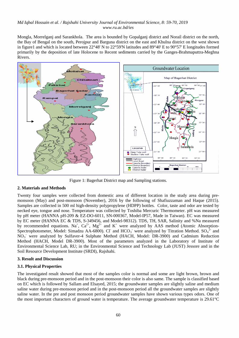
Md Iqbal Hossain et al. / Rajshahi University Journal of Environmental Science, 8: 59-70, 2019 www.ru.ac.bd/ies
60
Mongla, Morrelganj and Sarankhola. The area is bounded by Gopalganj district and Norail district on the north, the Bay of Bengal on the south, Perojpur and Barguna district on the east and Khulna district on the west shown in figure1 and which is located between 22°48' N to 22°59'N latitudes and 89°40' E to 90°57' E longitudes formed primarily by the deposition of late Holocene to Recent sediments carried by the Ganges-Brahmaputtra-Meghna Rivers.
Figure 1: Bagerhat District map and Sampling stations.
2. Materials and Methods
Twenty four samples were collected from domestic area of different location in the study area during pre-monsoon (May) and post-monsoon (November), 2016 by the following of Shafiuzzaman and Haque (2015). Samples are collected in 500 ml high-density polypropylene (HDPP) bottles. Color, taste and odor are tested by necked eye, tongue and nose. Temperature was collected by Toshiba Mercuric Thermometer. pH was measured by pH meter (HANNA pH-209 & EZ-DO-6011, SN-000367, Model-IP57, Made in Taiwan). EC was measured by EC meter (HANNA EC & TDS, S-349456, and Model-98312). TDS, TH, SAR, Salinity and %Na measured by recommended equations. Na+, Ca2+, Mg2+ and K+ were analyzed by AAS method (Atomic Absorption-Spectrophotometer, Model: Simadzu AA-6800). Cl- and HCO3
- were analyzed by Titration Method. SO42- and
NO3- were analyzed by Sulfaver-4 Sulphate Method (HACH, Model: DR-3900) and Cadmium Reduction
Method (HACH, Model DR-3900). Most of the parameters analyzed in the Laboratory of Institute of Environmental Science Lab, RU; in the Environmental Science and Technology Lab (JUST) Jessore and in the Soil Resource Development Institute (SRDI), Rajshahi.
3. Result and Discussion
3.1. Physical Properties
The investigated result showed that most of the samples color is normal and some are light brown, brown and black during pre-monsoon period and in the post-monsoon their color is also same. The sample is classified based on EC which is followed by Sallam and Elsayed, 2015; the groundwater samples are slightly saline and medium saline water during pre-monsoon period and in the post-monsoon period all the groundwater samples are slightly saline water. In the pre and post monsoon period groundwater samples have shown various types odors. One of the most important characters of ground water is temperature. The average groundwater temperature is 29.61°C
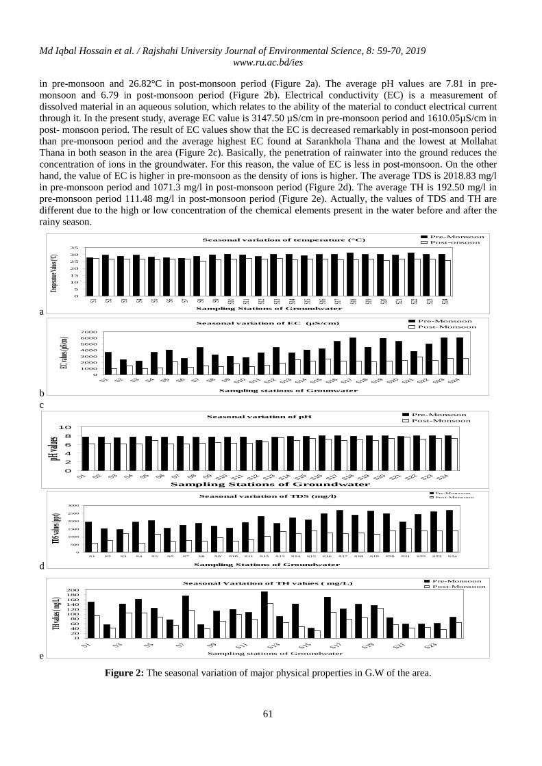
Md Iqbal Hossain et al. / Rajshahi University Journal of Environmental Science, 8: 59-70, 2019 www.ru.ac.bd/ies
61
in pre-monsoon and 26.82°C in post-monsoon period (Figure 2a). The average pH values are 7.81 in pre-monsoon and 6.79 in post-monsoon period (Figure 2b). Electrical conductivity (EC) is a measurement of dissolved material in an aqueous solution, which relates to the ability of the material to conduct electrical current through it. In the present study, average EC value is 3147.50 µS/cm in pre-monsoon period and 1610.05µS/cm in post- monsoon period. The result of EC values show that the EC is decreased remarkably in post-monsoon period than pre-monsoon period and the average highest EC found at Sarankhola Thana and the lowest at Mollahat Thana in both season in the area (Figure 2c). Basically, the penetration of rainwater into the ground reduces the concentration of ions in the groundwater. For this reason, the value of EC is less in post-monsoon. On the other hand, the value of EC is higher in pre-monsoon as the density of ions is higher. The average TDS is 2018.83 mg/l in pre-monsoon period and 1071.3 mg/l in post-monsoon period (Figure 2d). The average TH is 192.50 mg/l in pre-monsoon period 111.48 mg/l in post-monsoon period (Figure 2e). Actually, the values of TDS and TH are different due to the high or low concentration of the chemical elements present in the water before and after the rainy season.
a
bc
d
e
Figure 2: The seasonal variation of major physical properties in G.W of the area.
Seasonal variation of temperature (°C)
0
5
10
15
20
25
30
35
S1 S2 S3 S4 S5 S6 S7 S8 S9 S10 S11 S12 S13 S14 S15 S16 S17 S18 S19 S20 S21 S22 S23 S24
Sampling Stations of Groundwater
Tempera
ture Val
ues (°C)
Pre-MonsoonPost-onsoon
Seasonal variation of EC (µS/cm)
0
1000
2000
3000
4000
5000
6000
7000
S1 S2 S3 S4 S5 S6 S7 S8 S9 S10 S11 S12 S13 S14 S15 S16 S17 S18 S19 S20 S21 S22 S23 S24
Sampling stations of Grounwater
EC value
s (µS/cm)
Pre-MonsoonPost-Monsoon
Seasonal variation of pH
0
2
4
6
8
10
S1 S2 S3 S4 S5 S6 S7 S8 S9 S10 S11 S12 S13 S14 S15 S16 S17 S18 S19 S20 S21 S22 S23 S24Sampling Stations of Groundwater
pH valu
es
Pre-MonsoonPost-Monsoon
Seasonal variation of TDS (mg/l)
0
500
1000
1500
2000
2500
3000
S1 S2 S3 S4 S5 S6 S7 S8 S9 S10 S11 S12 S13 S14 S15 S16 S17 S18 S19 S20 S21 S22 S23 S24
Sampling Stations of Groundwater
TDS valu
es (ppt)
Pre-MonsoonPost-Monsoon
Seasonal Variation of TH values ( mg/L)
020406080
100120140160180200
S1 S3 S5 S7 S9 S11 S13 S15 S17 S19 S21 S23Sampling stations of Groundwater
TH valu
es ( mg/
L)
Pre-MonsoonPost-Monsoon
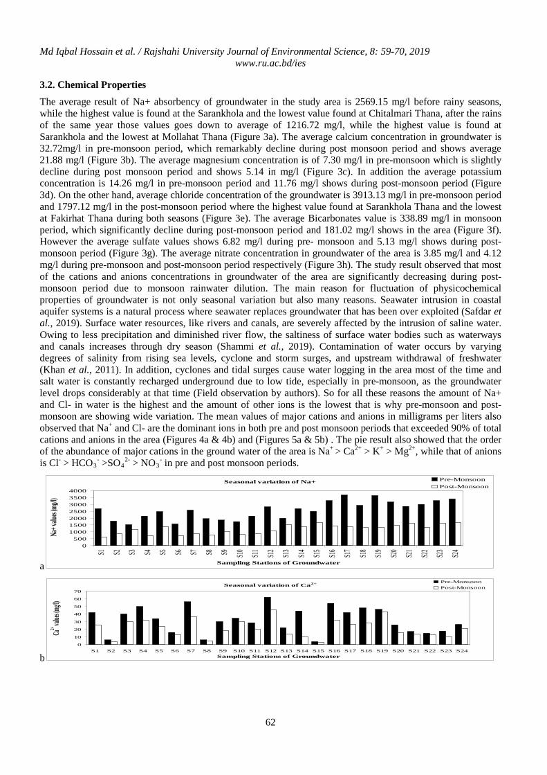
Md Iqbal Hossain et al. / Rajshahi University Journal of Environmental Science, 8: 59-70, 2019 www.ru.ac.bd/ies
62
3.2. Chemical Properties
The average result of Na+ absorbency of groundwater in the study area is 2569.15 mg/l before rainy seasons, while the highest value is found at the Sarankhola and the lowest value found at Chitalmari Thana, after the rains of the same year those values goes down to average of 1216.72 mg/l, while the highest value is found at Sarankhola and the lowest at Mollahat Thana (Figure 3a). The average calcium concentration in groundwater is 32.72mg/l in pre-monsoon period, which remarkably decline during post monsoon period and shows average 21.88 mg/l (Figure 3b). The average magnesium concentration is of 7.30 mg/l in pre-monsoon which is slightly decline during post monsoon period and shows 5.14 in mg/l (Figure 3c). In addition the average potassium concentration is 14.26 mg/l in pre-monsoon period and 11.76 mg/l shows during post-monsoon period (Figure 3d). On the other hand, average chloride concentration of the groundwater is 3913.13 mg/l in pre-monsoon period and 1797.12 mg/l in the post-monsoon period where the highest value found at Sarankhola Thana and the lowest at Fakirhat Thana during both seasons (Figure 3e). The average Bicarbonates value is 338.89 mg/l in monsoon period, which significantly decline during post-monsoon period and 181.02 mg/l shows in the area (Figure 3f). However the average sulfate values shows 6.82 mg/l during pre- monsoon and 5.13 mg/l shows during post-monsoon period (Figure 3g). The average nitrate concentration in groundwater of the area is 3.85 mg/l and 4.12 mg/l during pre-monsoon and post-monsoon period respectively (Figure 3h). The study result observed that most of the cations and anions concentrations in groundwater of the area are significantly decreasing during post-monsoon period due to monsoon rainwater dilution. The main reason for fluctuation of physicochemical properties of groundwater is not only seasonal variation but also many reasons. Seawater intrusion in coastal aquifer systems is a natural process where seawater replaces groundwater that has been over exploited (Safdar et al., 2019). Surface water resources, like rivers and canals, are severely affected by the intrusion of saline water. Owing to less precipitation and diminished river flow, the saltiness of surface water bodies such as waterways and canals increases through dry season (Shammi et al., 2019). Contamination of water occurs by varying degrees of salinity from rising sea levels, cyclone and storm surges, and upstream withdrawal of freshwater (Khan et al., 2011). In addition, cyclones and tidal surges cause water logging in the area most of the time and salt water is constantly recharged underground due to low tide, especially in pre-monsoon, as the groundwater level drops considerably at that time (Field observation by authors). So for all these reasons the amount of Na+ and Cl- in water is the highest and the amount of other ions is the lowest that is why pre-monsoon and post-monsoon are showing wide variation. The mean values of major cations and anions in milligrams per liters also observed that Na+ and Cl- are the dominant ions in both pre and post monsoon periods that exceeded 90% of total cations and anions in the area (Figures 4a & 4b) and (Figures 5a & 5b) . The pie result also showed that the order of the abundance of major cations in the ground water of the area is Na+ > Ca2+ > K+ > Mg2+, while that of anions is Cl- > HCO3
- >SO42- > NO3
- in pre and post monsoon periods.
a
b
Seasonal variation of Na+
0500
1000150020002500300035004000
S1 S2 S3 S4 S5 S6 S7 S8 S9 S10 S11 S12 S13 S14 S15 S16 S17 S18 S19 S20 S21 S22 S23 S24
Sampling Stations of Groundwater
Na+ v
alues (
mg/l)
Pre-MonsoonPost-Monsoon
Seasonal variation of Ca2+
0
10
20
30
40
50
60
70
S1 S2 S3 S4 S5 S6 S7 S8 S9 S10 S11 S12 S13 S14 S15 S16 S17 S18 S19 S20 S21 S22 S23 S24Sampling Stations of Groundwater
Ca2+ value
s (mg/l)
Pre-MonsoonPost-Monsoon
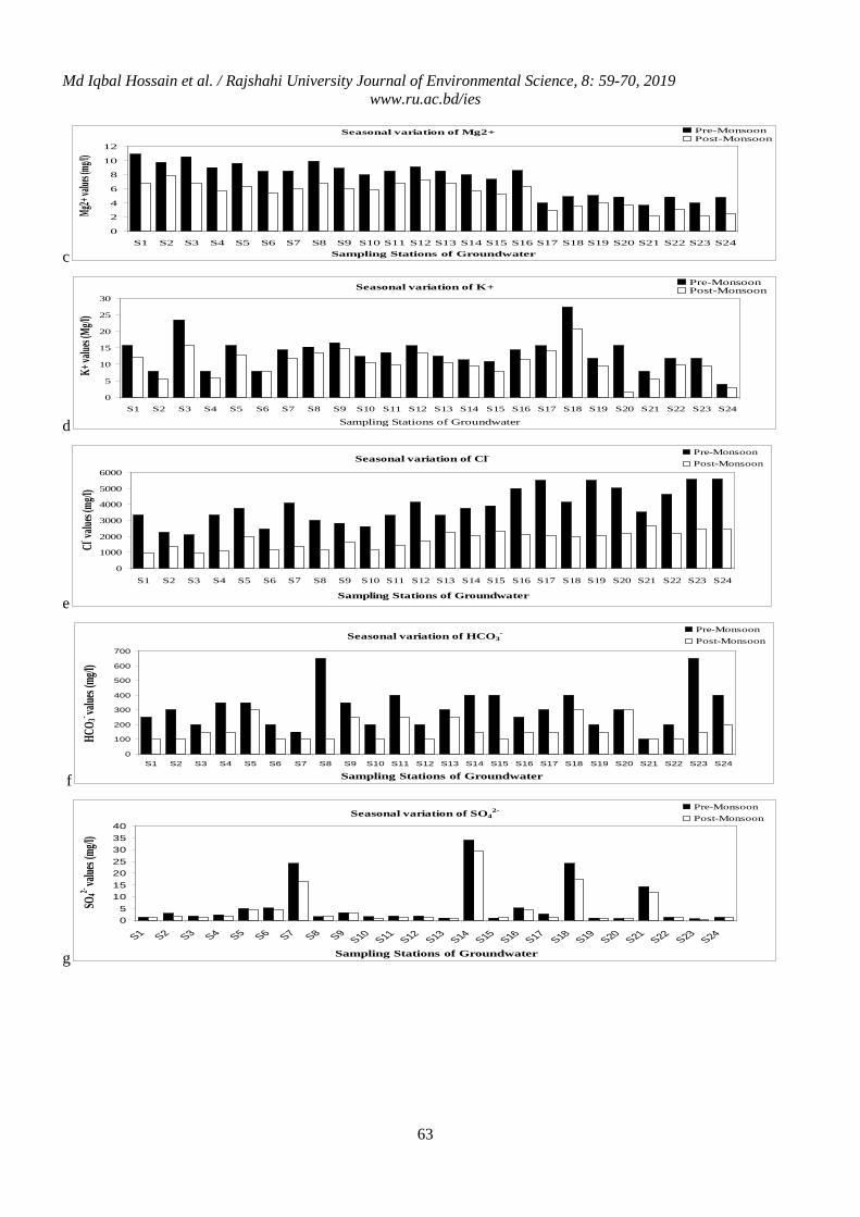
Md Iqbal Hossain et al. / Rajshahi University Journal of Environmental Science, 8: 59-70, 2019 www.ru.ac.bd/ies
63
c
d
e
f
g
Seasonal variation of Mg2+
0
2
4
6
8
10
12
S1 S2 S3 S4 S5 S6 S7 S8 S9 S10 S11 S12 S13 S14 S15 S16 S17 S18 S19 S20 S21 S22 S23 S24Sampling Stations of Groundwater
Mg2+
values
(mg/l)
Pre-MonsoonPost-Monsoon
Seasonal variation of K+
0
5
10
15
20
25
30
S1 S2 S3 S4 S5 S6 S7 S8 S9 S10 S11 S12 S13 S14 S15 S16 S17 S18 S19 S20 S21 S22 S23 S24
Sampling Stations of Groundwater
K+ va
lues (M
g/l)
Pre-MonsoonPost-Monsoon
Seasonal variation of Cl-
0
1000
2000
3000
4000
5000
6000
S1 S2 S3 S4 S5 S6 S7 S8 S9 S10 S11 S12 S13 S14 S15 S16 S17 S18 S19 S20 S21 S22 S23 S24
Sampling Stations of Groundwater
Cl- value
s (mg/l
)
Pre-MonsoonPost-Monsoon
Seasonal variation of HCO3-
0
100
200
300
400
500
600
700
S1 S2 S3 S4 S5 S6 S7 S8 S9 S10 S11 S12 S13 S14 S15 S16 S17 S18 S19 S20 S21 S22 S23 S24
Sampling Stations of Groundwater
HCO 3
- value
s (mg
/l)
Pre-MonsoonPost-Monsoon
Seasonal variation of SO42-
05
10152025303540
S1 S2 S3 S4 S5 S6 S7 S8 S9S10 S11 S12 S13 S14 S15 S16 S17 S18 S19 S20 S21 S22 S23 S24
Sampling Stations of Groundwater
SO42-
value
s (mg
/l)
Pre-MonsoonPost-Monsoon
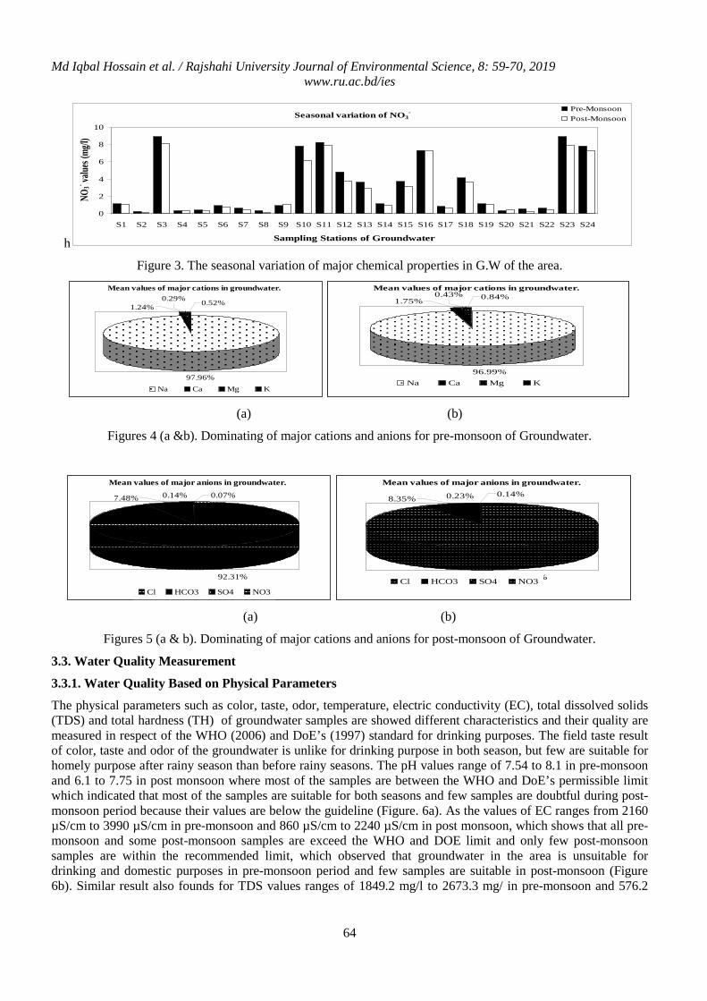
Md Iqbal Hossain et al. / Rajshahi University Journal of Environmental Science, 8: 59-70, 2019 www.ru.ac.bd/ies
64
h
Figure 3. The seasonal variation of major chemical properties in G.W of the area.
(a) (b)
Figures 4 (a &b). Dominating of major cations and anions for pre-monsoon of Groundwater.
(a) (b)
Figures 5 (a & b). Dominating of major cations and anions for post-monsoon of Groundwater. 3.3. Water Quality Measurement
3.3.1. Water Quality Based on Physical Parameters
The physical parameters such as color, taste, odor, temperature, electric conductivity (EC), total dissolved solids (TDS) and total hardness (TH) of groundwater samples are showed different characteristics and their quality are measured in respect of the WHO (2006) and DoE’s (1997) standard for drinking purposes. The field taste result of color, taste and odor of the groundwater is unlike for drinking purpose in both season, but few are suitable for homely purpose after rainy season than before rainy seasons. The pH values range of 7.54 to 8.1 in pre-monsoon and 6.1 to 7.75 in post monsoon where most of the samples are between the WHO and DoE’s permissible limit which indicated that most of the samples are suitable for both seasons and few samples are doubtful during post-monsoon period because their values are below the guideline (Figure. 6a). As the values of EC ranges from 2160 µS/cm to 3990 µS/cm in pre-monsoon and 860 µS/cm to 2240 µS/cm in post monsoon, which shows that all pre-monsoon and some post-monsoon samples are exceed the WHO and DOE limit and only few post-monsoon samples are within the recommended limit, which observed that groundwater in the area is unsuitable for drinking and domestic purposes in pre-monsoon period and few samples are suitable in post-monsoon (Figure 6b). Similar result also founds for TDS values ranges of 1849.2 mg/l to 2673.3 mg/ in pre-monsoon and 576.2
Seasonal variation of NO3-
0
2
4
6
8
10
S1 S2 S3 S4 S5 S6 S7 S8 S9 S10 S11 S12 S13 S14 S15 S16 S17 S18 S19 S20 S21 S22 S23 S24
Sampling Stations of Groundwater
NO3- va
lues (
mg/l)
Pre-MonsoonPost-Monsoon
Mean values of major cations in groundwater.
0.52%0.29%1.24%
97.96%Na Ca Mg K
Mean values of major cations in groundwater.0.84%0.43%
1.75%
96.99%Na Ca Mg K
Mean values of major anions in groundwater.
92.31%
7.48% 0.14% 0.07%
Cl HCO3 SO4 NO3
Mean values of major anions in groundwater.0.14%0.23%8.35%
91.28%Cl HCO3 SO4 NO3
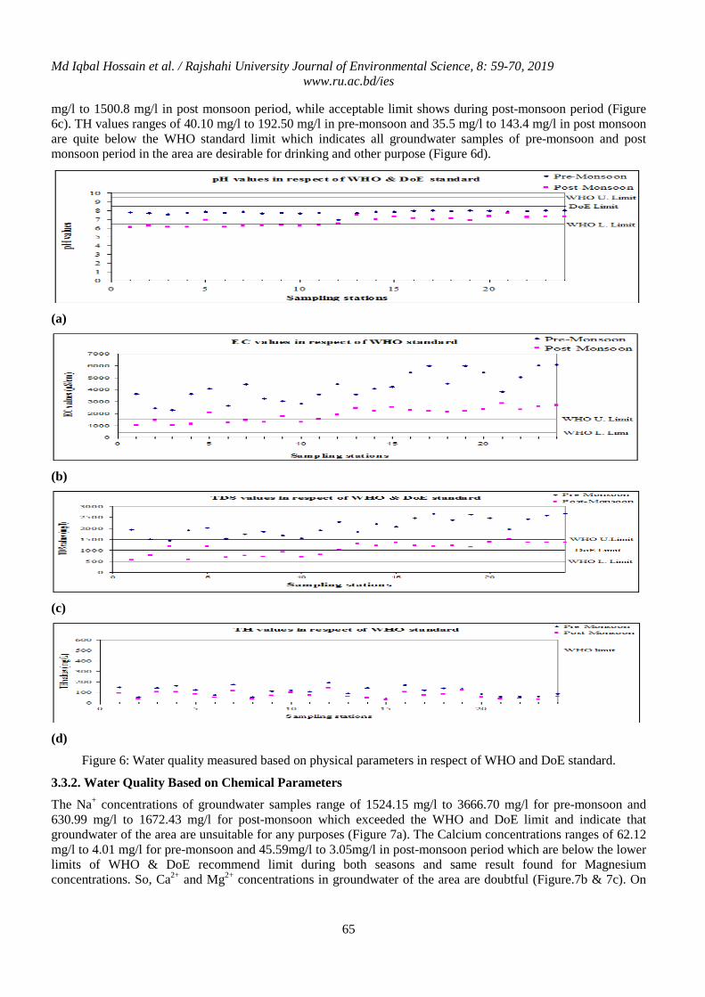
Md Iqbal Hossain et al. / Rajshahi University Journal of Environmental Science, 8: 59-70, 2019 www.ru.ac.bd/ies
65
mg/l to 1500.8 mg/l in post monsoon period, while acceptable limit shows during post-monsoon period (Figure 6c). TH values ranges of 40.10 mg/l to 192.50 mg/l in pre-monsoon and 35.5 mg/l to 143.4 mg/l in post monsoon are quite below the WHO standard limit which indicates all groundwater samples of pre-monsoon and post monsoon period in the area are desirable for drinking and other purpose (Figure 6d).
(a)
(b)
(c)
(d)
Figure 6: Water quality measured based on physical parameters in respect of WHO and DoE standard.
3.3.2. Water Quality Based on Chemical Parameters
The Na+ concentrations of groundwater samples range of 1524.15 mg/l to 3666.70 mg/l for pre-monsoon and 630.99 mg/l to 1672.43 mg/l for post-monsoon which exceeded the WHO and DoE limit and indicate that groundwater of the area are unsuitable for any purposes (Figure 7a). The Calcium concentrations ranges of 62.12 mg/l to 4.01 mg/l for pre-monsoon and 45.59mg/l to 3.05mg/l in post-monsoon period which are below the lower limits of WHO & DoE recommend limit during both seasons and same result found for Magnesium concentrations. So, Ca2+ and Mg2+ concentrations in groundwater of the area are doubtful (Figure.7b & 7c). On
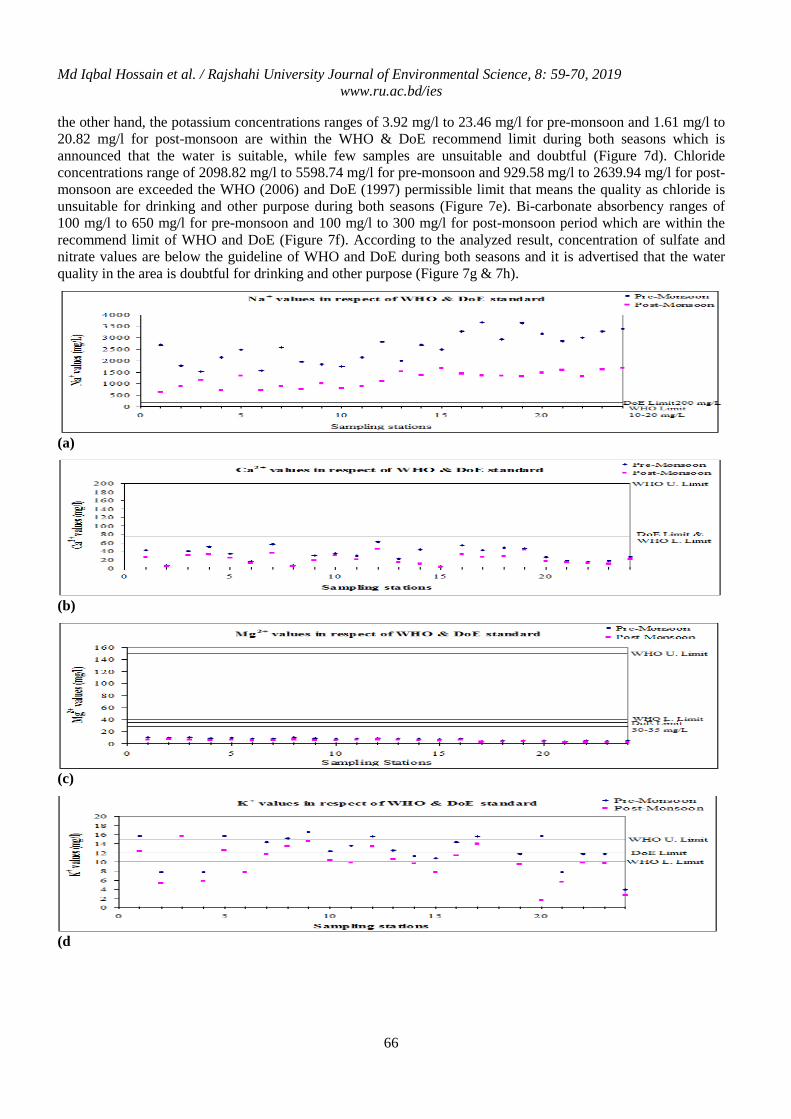
Md Iqbal Hossain et al. / Rajshahi University Journal of Environmental Science, 8: 59-70, 2019 www.ru.ac.bd/ies
66
the other hand, the potassium concentrations ranges of 3.92 mg/l to 23.46 mg/l for pre-monsoon and 1.61 mg/l to 20.82 mg/l for post-monsoon are within the WHO & DoE recommend limit during both seasons which is announced that the water is suitable, while few samples are unsuitable and doubtful (Figure 7d). Chloride concentrations range of 2098.82 mg/l to 5598.74 mg/l for pre-monsoon and 929.58 mg/l to 2639.94 mg/l for post-monsoon are exceeded the WHO (2006) and DoE (1997) permissible limit that means the quality as chloride is unsuitable for drinking and other purpose during both seasons (Figure 7e). Bi-carbonate absorbency ranges of 100 mg/l to 650 mg/l for pre-monsoon and 100 mg/l to 300 mg/l for post-monsoon period which are within the recommend limit of WHO and DoE (Figure 7f). According to the analyzed result, concentration of sulfate and nitrate values are below the guideline of WHO and DoE during both seasons and it is advertised that the water quality in the area is doubtful for drinking and other purpose (Figure 7g & 7h).
(a)
(b)
(c)
(d
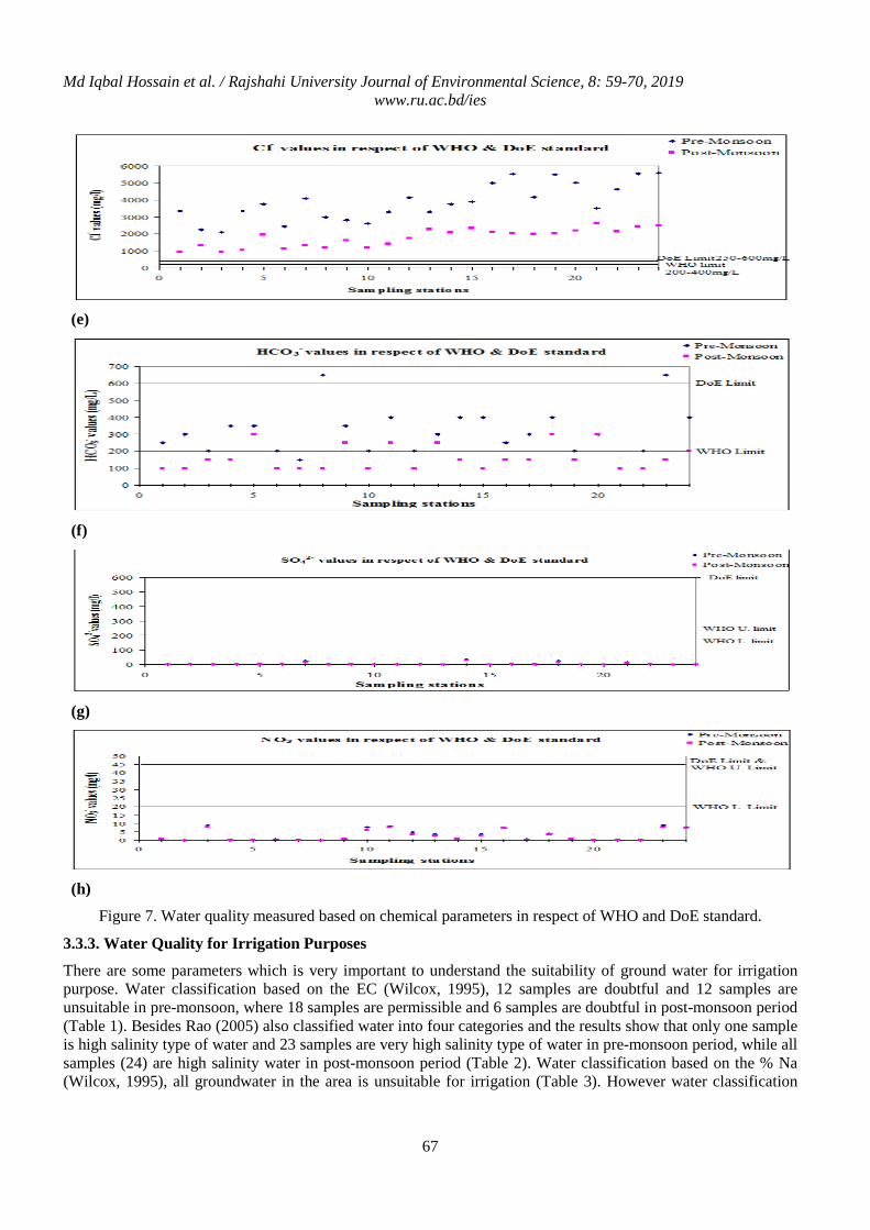
Md Iqbal Hossain et al. / Rajshahi University Journal of Environmental Science, 8: 59-70, 2019 www.ru.ac.bd/ies
67
(e)
(f)
(g)
(h)
Figure 7. Water quality measured based on chemical parameters in respect of WHO and DoE standard.
3.3.3. Water Quality for Irrigation Purposes
There are some parameters which is very important to understand the suitability of ground water for irrigation purpose. Water classification based on the EC (Wilcox, 1995), 12 samples are doubtful and 12 samples are unsuitable in pre-monsoon, where 18 samples are permissible and 6 samples are doubtful in post-monsoon period (Table 1). Besides Rao (2005) also classified water into four categories and the results show that only one sample is high salinity type of water and 23 samples are very high salinity type of water in pre-monsoon period, while all samples (24) are high salinity water in post-monsoon period (Table 2). Water classification based on the % Na (Wilcox, 1995), all groundwater in the area is unsuitable for irrigation (Table 3). However water classification
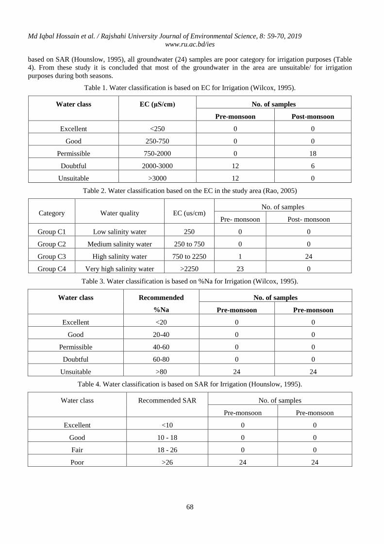
Md Iqbal Hossain et al. / Rajshahi University Journal of Environmental Science, 8: 59-70, 2019 www.ru.ac.bd/ies
68
based on SAR (Hounslow, 1995), all groundwater (24) samples are poor category for irrigation purposes (Table 4). From these study it is concluded that most of the groundwater in the area are unsuitable/ for irrigation purposes during both seasons.
Table 1. Water classification is based on EC for Irrigation (Wilcox, 1995).
Water class EC (μS/cm) No. of samples Pre-monsoon Post-monsoon
Excellent <250 0 0 Good 250-750 0 0
Permissible 750-2000 0 18 Doubtful 2000-3000 12 6
Unsuitable >3000 12 0 Table 2. Water classification based on the EC in the study area (Rao, 2005)
Category Water quality EC (us/cm) No. of samples
Pre- monsoon Post- monsoon Group C1 Low salinity water 250 0 0 Group C2 Medium salinity water 250 to 750 0 0 Group C3 High salinity water 750 to 2250 1 24 Group C4 Very high salinity water >2250 23 0
Table 3. Water classification is based on %Na for Irrigation (Wilcox, 1995).
Water class Recommended %Na
No. of samples Pre-monsoon Pre-monsoon
Excellent <20 0 0 Good 20-40 0 0
Permissible 40-60 0 0 Doubtful 60-80 0 0
Unsuitable >80 24 24 Table 4. Water classification is based on SAR for Irrigation (Hounslow, 1995).
Water class Recommended SAR No. of samples Pre-monsoon Pre-monsoon
Excellent <10 0 0 Good 10 - 18 0 0 Fair 18 - 26 0 0 Poor >26 24 24
Md Iqbal Hossain et al. / Rajshahi University Journal of Environmental Science, 8: 59-70, 2019 www.ru.ac.bd/ies
69
4. Conclusion
There is a lack of fresh water all over the world now. Bangladesh is no exception to it and coastal areas of Bangladesh are more vulnerable to salinity problem. Due to which the salinity of water in the coastal area is increasing. As a result water quality is deteriorating day by day. The evaluation of groundwater quality based on the physicochemical parameters concluded that all parameters are seasonally fluctuated, while most of the parameters remarkably decreased during post-monsoon period because most of the physicochemical properties concentrations in groundwater of the area are significantly decreasing during post-monsoon period due to monsoon rainwater dilution. Comparing of the most physicochemical properties of groundwater in the study area with WHO (2006) and DoE (1997) standard limits shows that some properties are acceptable in post-monsoon most of are unacceptable in pre-monsoon besides some are doubtful because their position is below the guideline. The groundwater quality for irrigation is compared based on electrical conductance (EC), per cent sodium (%Na) and sodium absorption ratio (SAR) shows that groundwater moderately unsuitable and poor quality for irrigation purposes, but little is suitable for irrigation in post-monsoon period according to EC values (Wilcox, 1995). So the study result concluded that most of the groundwater in the area is unsuitable or objectionable for drinking, domestic and irrigation purposes during both seasons. That is why the lives of the people of the coastal area are being severely damaged as well as the country’s economy. The coastal people and the government need a lot of support to maintain the quality of groundwater. However some techniques such as prevention of seawater intrusion, rainwater harvesting, land pattern changing, decreasing pumping of tube well, making embankment can create a comparative better way to find suitable water for various purposes for future generation.
References
Ahmed I, Kadir NM and Ahmed HM. 2014. Intrusion of surface water salinity in the Western Coastal belt of
Bangladesh. Inter. J. Environ. Pollut. and Ctrl. Res., 1:7–12.
Azaza HF, Ketata M, Bouhlila R, Gueddari M and Riberio L. 2011. Hydrogeochemical characteristics and assessment of drinking water quality in Zeuss–Koutine aquifer, southeastern Tunisia. Environ Monit Assess,174 (1–4): 283–298 (16).
P&HC (Population & Housing Census) 2011. Community Report on Bagerhat, Bagerhat, Bd: Bangladesh Bureau of Statistics and Informatics Division.
DoE (Department of Environment) 1997. Notification of the Environment Conservation Rules, Ministry of Environment and Forest.
Hosseinifard JS and Aminiyan MM. 2015. Hydrochemical Characterization of Groundwater Quality for Drinking and Agricultural Purposes: A Case Study in Rafsanjan Plain, Iran. Water Quality, Exposure and Health, 7:531–544 (14).
Hounslow AW. 1995. Water quality data analysis and interpretation: Lewis publishers, CRC Press, Taylor and Francis group, London. 416p.
Islam M A, Zahid A, Rahman MM, Rahman SM, Islam JM, Akter Y, Shammi M, Doza BM and Roy B. 2016. Investigation of Groundwater Quality and Its Suitability for Drinking and Agricultural Use in the South
Central Part of the Coastal Region in Bangladesh. Expo Health, 1-16 (16).
Khan EA, Ireson A, Kovats S, Mojumder S, Khusru A, Rahman A and Vineis P. 2011. Drinking water salinity and maternal health in coastal Bangladesh: Implications of climate change. Environ Health Perspect., 119:1328–1332(5).
Nickson TR, Shrestha B, .Kyaw-Myint OT and Lowry D. 2005. Arsenic and others drinking quality issues, Muzaffargarh district, Pakistan. Appl. Geochem, 20 (1): 55-68(14).
Rani LA and Babu SSD. 2007. A statistical evaluation of groundwater chemistry from the west coast of Tamil Nadu, India. Ind. J. Marine Sci., 37: 186-192.
Md Iqbal Hossain et al. / Rajshahi University Journal of Environmental Science, 8: 59-70, 2019 www.ru.ac.bd/ies
70
Rao NS. 2005. Seasonal variation of groundwater quality in a part of Guntur District, Andhra Pradesh, India. Environ Geol., 49: 413–429.
Safdar H, Amin A, Shafiq Y, Ali A, Yasin R, Shoukat A, Hussan M and Sarwar IM. 2019. A review: Impact of salinity on plant growth. Nat Sci., 17 (1): 34-40 (7).
Sallam GAH and Elsayed EA. 2015. Estimating relations between temperature, relative humidity as independed variables and selected water quality parameters in Lake Manzala, Egypt. Ain Shams Engrg. J., 1-14.
Shafiuzzaman MS. and Haque EK. 2015. Impact of water salinity on major crops production in most of the coastal adjoining area of Satkhira district, Bangladesh. Rajshahi. Uni. J. Environ. Sci., 3: 27-32.
Shammi M, Rahman MM Bondad ES and Doza BM. 2019. Impacts of Salinity Intrusion in Community Health: A Review of Experiences on Drinking Water Sodium from Coastal Areas of Bangladesh. Healthcare, 7 (50): 1-19(19).
WHO (World Health Organization) 2006. Guideline for drinking water quality Vol:-I., Geneva.
Wilcox LV. 1995. Classification and use of irrigation waters. US Department of Agriculture, Washington Dc, p-19.
Md. Mokhlesur Rahman et al. / Rajshahi University Journal of Environmental Science, 8: 71-78, 2019 www.ru.ac.bd/ies
Usages and Impacts of Quinalphos in Commercial Aquaculture in Rajshahi, Bangladesh
Md. Mokhlesur Rahman1∗ and M. Nazrul Islam2
1Institute of Environmental Science, University of Rajshahi, Rajshahi-6205, Bangladesh.
2Department of Zoology, University of Rajshahi, Rajshahi-6205, Bangladesh
Abstract Fish farmers involved in commercial aquaculture in northwest Bangladesh is striving for ruthless efficiency of the system. In this process they have been selective poisoning the undesired species (!) by using quinalphos pesticides while keeping their desired species (Indian and Chinese major carps) seemingly unaffected. The study was conducted to know the impact of the use of quinalphos on zooplankton, aquatic insects and benthos population in commercial aquaculture ponds. To know the bioaccumulation phenomena, fish were collected pre and post-treatment and analyzed for residual content of quinalphos. Zooplankton, aquatic insects and benthos sample were collected and counted at pretreatment and after 1 day, 2 days, 5 days, 10 days, 15 days, 21 days and 28 days after the treatment. Quinalphos was found to be bioaccumulated in fish till 10 days after the use. Zooplankton were found to be impacted for short duration and were able to regenerate within 5 days of the use of quinalphos. Aquatic insects and benthos were also affected but the loss of insect diversity was observed till the end of the observation period.
Keywords: Quinalphos; Selective poisoning; Aquaculture; Bioaccumulation; Zooplankton; Aquatic insects.
1. Introduction
The activity of commercial aquaculture begins with complete wipeout of existing batch of left-over fish (that didn’t come under catchment as live) and water insects from the pond using various chemicals (like starting with a clean sheet), which is followed by stocking of desired number of relatively large fish (Indian major carps of 0.5 kg to 1.5 kg in size)in northwest Bangladesh compared to the other parts of the country. In the process of transferring the live fish from the nursery pond to the stocking pond, undesired (!) small indigenous fish species like Pseudambasis sp., Chanda sp., Glossogobius sp. and Puntius sp. etc. also get transferred unintentionally by the farmers into the stocking pond. Since these small indigenous species can breed in ponds, within few months (especially after monsoon) they manage to multiply and populate the culture ponds of Indian major carps. Despite of the disparity of the size between these indigenous species and large Indian and Chinese major carps (more than 1.5 kg in size) in commercial ponds, farm owners view these small species as a challenge to the desired species that might face competition for food and space or at least get disturbed by these tiny fish. Some fish like Chanda sp. and Pseudambasis sp.(which usually present in large number) does keep biting and feeding on scales of carps, especially silver carps with their jaws that is armed with curved and conical teeth (Wahab, 2003) and thus make the carp fish scale less glossy, will reduce the price in the market if sold, apart from the risk of hampering the growth.On the other hand, Glossogobius sp. is a voracious feeder and almost feeds on everything namely decaying organic matter, protozoans, planktons, water insects, other fish and their eggs and larvae (Siddiqui et al., 2007). Thus Glossogobius sp. can create competition for feed supplied to the commercial aquaculture pond.
Quinalphos is a broad-spectrum organophosphate insecticide with contact and stomach action used against common pests like aphids, caterpillars, mealybugs, mites, bollworms, leafhoppers and borers of various crops and plants like wheat, sugarcane, peanut, sorghum, cotton, fiber-crops etc. has been in widespread use since 1970 (IUPAC, 2019). National Center for Biotechnology Information (NCBI) (2019) has categorized the toxicity of quinalphos as ‘very toxic to aquatic life’ and ‘very toxic to aquatic life with long lasting effects’. Despite being labeled as very toxic, it has a wide range when comes to the toxicity to fish, that means for some fish tolerance level of quinalphos is way higher than others even within the same family of fish. For example, regarding quinalphos, 96 hour LC50 value of silver barb (Barbonymus gonionotus) is 4.70 mg/l (Mostakim et al., 2014), of Labeorohita is 2.826 mg/l (Rathnamma and Nagaraju, 2013), of Cyprinuscarpio is 2.75 mg/l (Padmanabha et al., 2016), of Catlacatla is 2.91mg/l (Rajput, 2012), of Cirrhinus mrigala is 0.128mg/l (Nair et al., 2017) and of ∗ Corresponding author’s e-mail: [email protected]
Md. Mokhlesur Rahman et al. / Rajshahi University Journal of Environmental Science, 8: 71-78, 2019 www.ru.ac.bd/ies
72
Oncorhynchus mykiss is 0.005 mg/l (IUPAC, 2019). Therefore, a given dose (depending on the dose itself) may be very toxic to one fish species while may not be harmful at all for another species. This phenomenon of quinalphos is exploited by the commercial fish farmers in northwest Bangladesh and quinalphos is being used as a weapon (selective poison) to kill and wipeout the undesired (!) fish species like Chanda sp., Pseudambasis sp. and Glossogobius sp. Though the author failed to find any reference for LC50 value of Pseudambasis sp. and Glossogobius sp. for quinalphos but that is defiantly much lower than that of Indian major carps in commercial aquaculture ponds. The study was conducted to know the unintended consequences of use of quinalphos in commercial aquaculture ponds on fish, zooplankton, aquatic insects and benthos population.
2. Materials and Methods
The study was conducted in 3 different ponds (each of which were 2 to 3 acres in size) under commercial aquaculture located in Hatgodagari area of Pobaupazilla of Rajshahi. During the survey in the region the author came to know about this practice by the farmers. Therefore, farmers were communicated early to inform the author when they intend to use quinalphos in culture ponds. Accordingly, the author was present during the treatment in last week of November 2018. Total quantity of quinalphos pesticide was diluted in a big aluminum pot and then was broadcasted manually over the entire body of water of the pond. Based on the uses the doses were back calculated using the following formula: Concentration (mg/liter) = total amount of pure quinalphos (in mg) / volume of the water (of the pond in liter). Accordingly, the doses of quinalphos were found to be 0.02 mg/liter which is little less than 1/6th of the (lowest of Indian major carps) 96-hour LC50 value of Cirrhinus mrigala (LC50 value is 0.128 mg/l). The study was repeated using similar doses of quinalphos (brand name Deviqueen 25 EC quinalphos marketed by ‘The Limit Agroproducts Ltd’) with two additional farmers at different times and each one/pond was considered as one replication. Sampling of zooplankton, aquatic insects and benthos was done just before the treatment and 1 day, 2 days, 5 days, 10 days, 15 days, 21 days and 28 days after the treatment. In addition, fish and water sample were also collected pretreatment and after 1 day, 2 days, 5 days and 10 days of the experiment for testing the residue level of quinalphos. For each sampling approximately one to one and half kg fish (Labeo rohita) were caught using cast net, put in a plastic bag and immediately transferred into the freezer. Water samples were collected from 18 inches below the surface of water level, at least from four different locations of the pond to make totaling of 1 liter. The water sample was put in non-transparent plastic bottle and immediately put into the freezer. Both the fish and water samples were coded with numbers and transferred to the ‘Pesticide Analytical Laboratory’ located in Entomology Division of Bangladesh Agricultural Research Institute (BARI). The lab then analyzed the sampleusing GCMS-MS machine (level of detection of organophosphate insecticides ranged from 0.003 to 0.009 mg/liter) for quinalphos residue and delivered the report.
2.1. Sampling of Zooplankton
Zooplankton sampling was done using a plankton net (specification- 200 US with 75 to 85 microns mesh size). The plankton net had a circular mouth/head fitted with a metal frame used as inlet. The opposite side of the opening has a tapering end fitted with a collection bottle. The net was towed through the pond water one feet below the surface for certain distance. Based on the traversed distance and radius of the opening end of the net, total volume of pond water sieved through the net was calculated. Then the collected zooplankton sample was taken into a plastic bottle. The sample in plastic bottle now represents the total volume of water sieved through the net. 5% formalin was added in the plastic bottle with sample for fixation and preservation of the planktons till they were taken to the lab, identified and counted using a Sedgewick-Rafter cell counter (Welch, 1948) under microscope. Based on the counting, volume of stock sample in plastic bottle and the total volume of water from where the sample was collected, zooplankton concentration (nos/liter of pond water) was calculated.
2.2. Sampling of Aquatic Insects
For collection of aquatic insects, a fine meshed net fitted with a square meter frame was towed for three meters along the edges of the pond. The collected insects were then transferred in a plastic bottle and 5% formalin was added for the preservation of the sample. Then it was taken to the lab where all insects were identified and counted.
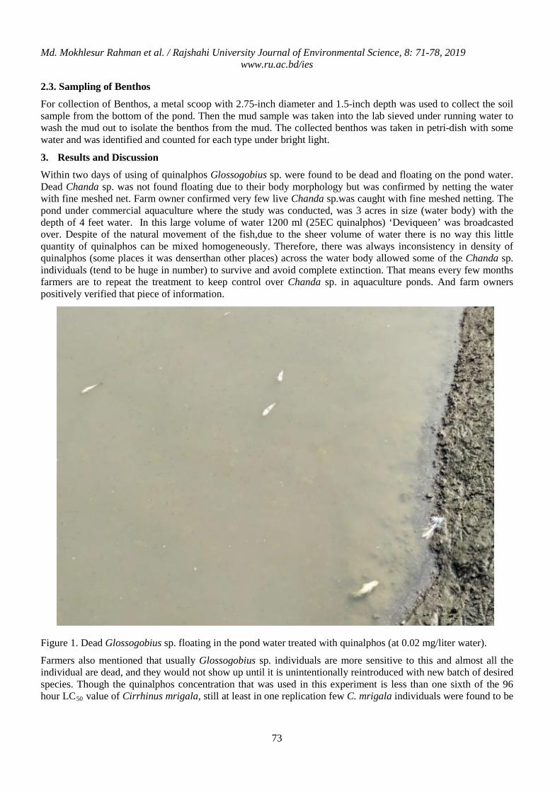
Md. Mokhlesur Rahman et al. / Rajshahi University Journal of Environmental Science, 8: 71-78, 2019 www.ru.ac.bd/ies
73
2.3. Sampling of Benthos
For collection of Benthos, a metal scoop with 2.75-inch diameter and 1.5-inch depth was used to collect the soil sample from the bottom of the pond. Then the mud sample was taken into the lab sieved under running water to wash the mud out to isolate the benthos from the mud. The collected benthos was taken in petri-dish with some water and was identified and counted for each type under bright light.
3. Results and Discussion
Within two days of using of quinalphos Glossogobius sp. were found to be dead and floating on the pond water. Dead Chanda sp. was not found floating due to their body morphology but was confirmed by netting the water with fine meshed net. Farm owner confirmed very few live Chanda sp.was caught with fine meshed netting. The pond under commercial aquaculture where the study was conducted, was 3 acres in size (water body) with the depth of 4 feet water. In this large volume of water 1200 ml (25EC quinalphos) ‘Deviqueen’ was broadcasted over. Despite of the natural movement of the fish,due to the sheer volume of water there is no way this little quantity of quinalphos can be mixed homogeneously. Therefore, there was always inconsistency in density of quinalphos (some places it was denserthan other places) across the water body allowed some of the Chanda sp. individuals (tend to be huge in number) to survive and avoid complete extinction. That means every few months farmers are to repeat the treatment to keep control over Chanda sp. in aquaculture ponds. And farm owners positively verified that piece of information.
Figure 1. Dead Glossogobius sp. floating in the pond water treated with quinalphos (at 0.02 mg/liter water).
Farmers also mentioned that usually Glossogobius sp. individuals are more sensitive to this and almost all the individual are dead, and they would not show up until it is unintentionally reintroduced with new batch of desired species. Though the quinalphos concentration that was used in this experiment is less than one sixth of the 96 hour LC50 value of Cirrhinus mrigala, still at least in one replication few C. mrigala individuals were found to be
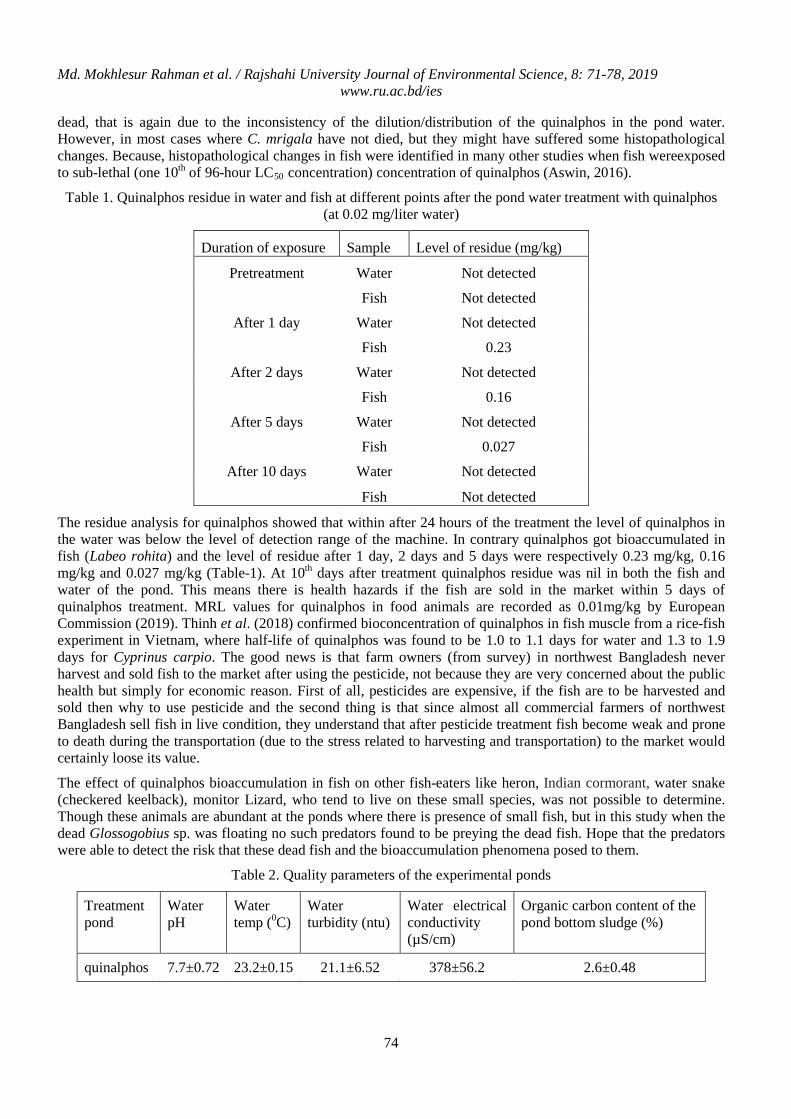
Md. Mokhlesur Rahman et al. / Rajshahi University Journal of Environmental Science, 8: 71-78, 2019 www.ru.ac.bd/ies
74
dead, that is again due to the inconsistency of the dilution/distribution of the quinalphos in the pond water. However, in most cases where C. mrigala have not died, but they might have suffered some histopathological changes. Because, histopathological changes in fish were identified in many other studies when fish wereexposed to sub-lethal (one 10th of 96-hour LC50 concentration) concentration of quinalphos (Aswin, 2016).
Table 1. Quinalphos residue in water and fish at different points after the pond water treatment with quinalphos (at 0.02 mg/liter water)
Duration of exposure Sample Level of residue (mg/kg) Pretreatment Water Not detected
Fish Not detected After 1 day Water Not detected
Fish 0.23 After 2 days Water Not detected
Fish 0.16 After 5 days Water Not detected
Fish 0.027 After 10 days Water Not detected
Fish Not detected The residue analysis for quinalphos showed that within after 24 hours of the treatment the level of quinalphos in the water was below the level of detection range of the machine. In contrary quinalphos got bioaccumulated in fish (Labeo rohita) and the level of residue after 1 day, 2 days and 5 days were respectively 0.23 mg/kg, 0.16 mg/kg and 0.027 mg/kg (Table-1). At 10th days after treatment quinalphos residue was nil in both the fish and water of the pond. This means there is health hazards if the fish are sold in the market within 5 days of quinalphos treatment. MRL values for quinalphos in food animals are recorded as 0.01mg/kg by European Commission (2019). Thinh et al. (2018) confirmed bioconcentration of quinalphos in fish muscle from a rice-fish experiment in Vietnam, where half-life of quinalphos was found to be 1.0 to 1.1 days for water and 1.3 to 1.9 days for Cyprinus carpio. The good news is that farm owners (from survey) in northwest Bangladesh never harvest and sold fish to the market after using the pesticide, not because they are very concerned about the public health but simply for economic reason. First of all, pesticides are expensive, if the fish are to be harvested and sold then why to use pesticide and the second thing is that since almost all commercial farmers of northwest Bangladesh sell fish in live condition, they understand that after pesticide treatment fish become weak and prone to death during the transportation (due to the stress related to harvesting and transportation) to the market would certainly loose its value.
The effect of quinalphos bioaccumulation in fish on other fish-eaters like heron, Indian cormorant, water snake (checkered keelback), monitor Lizard, who tend to live on these small species, was not possible to determine. Though these animals are abundant at the ponds where there is presence of small fish, but in this study when the dead Glossogobius sp. was floating no such predators found to be preying the dead fish. Hope that the predators were able to detect the risk that these dead fish and the bioaccumulation phenomena posed to them.
Table 2. Quality parameters of the experimental ponds
Treatment pond
Water pH
Water temp (0C)
Water turbidity (ntu)
Water electrical conductivity (µS/cm)
Organic carbon content of the pond bottom sludge (%)
quinalphos 7.7±0.72 23.2±0.15 21.1±6.52 378±56.2 2.6±0.48
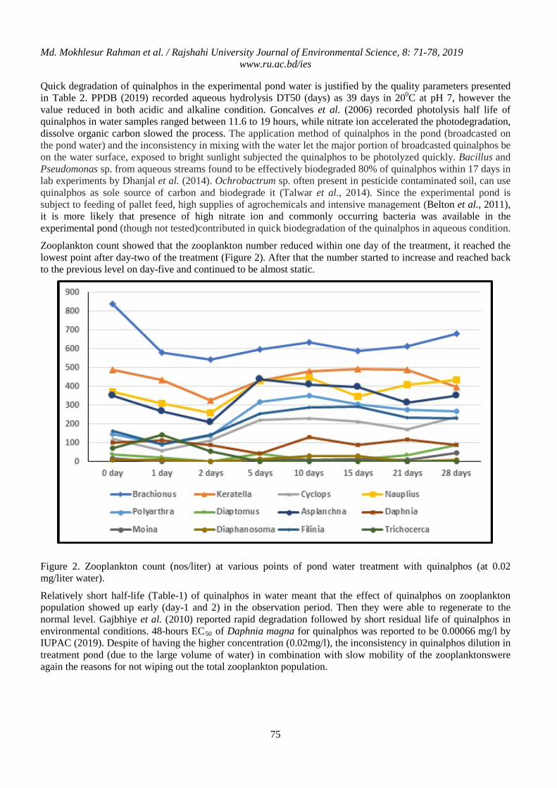
Md. Mokhlesur Rahman et al. / Rajshahi University Journal of Environmental Science, 8: 71-78, 2019 www.ru.ac.bd/ies
75
Quick degradation of quinalphos in the experimental pond water is justified by the quality parameters presented in Table 2. PPDB (2019) recorded aqueous hydrolysis DT50 (days) as 39 days in 200C at pH 7, however the value reduced in both acidic and alkaline condition. Goncalves et al. (2006) recorded photolysis half life of quinalphos in water samples ranged between 11.6 to 19 hours, while nitrate ion accelerated the photodegradation, dissolve organic carbon slowed the process. The application method of quinalphos in the pond (broadcasted on the pond water) and the inconsistency in mixing with the water let the major portion of broadcasted quinalphos be on the water surface, exposed to bright sunlight subjected the quinalphos to be photolyzed quickly. Bacillus and Pseudomonas sp. from aqueous streams found to be effectively biodegraded 80% of quinalphos within 17 days in lab experiments by Dhanjal et al. (2014). Ochrobactrum sp. often present in pesticide contaminated soil, can use quinalphos as sole source of carbon and biodegrade it (Talwar et al., 2014). Since the experimental pond is subject to feeding of pallet feed, high supplies of agrochemicals and intensive management (Belton et al., 2011), it is more likely that presence of high nitrate ion and commonly occurring bacteria was available in the experimental pond (though not tested)contributed in quick biodegradation of the quinalphos in aqueous condition.
Zooplankton count showed that the zooplankton number reduced within one day of the treatment, it reached the lowest point after day-two of the treatment (Figure 2). After that the number started to increase and reached back to the previous level on day-five and continued to be almost static.
Figure 2. Zooplankton count (nos/liter) at various points of pond water treatment with quinalphos (at 0.02 mg/liter water).
Relatively short half-life (Table-1) of quinalphos in water meant that the effect of quinalphos on zooplankton population showed up early (day-1 and 2) in the observation period. Then they were able to regenerate to the normal level. Gajbhiye et al. (2010) reported rapid degradation followed by short residual life of quinalphos in environmental conditions. 48-hours EC50 of Daphnia magna for quinalphos was reported to be 0.00066 mg/l by IUPAC (2019). Despite of having the higher concentration (0.02mg/l), the inconsistency in quinalphos dilution in treatment pond (due to the large volume of water) in combination with slow mobility of the zooplanktonswere again the reasons for not wiping out the total zooplankton population.
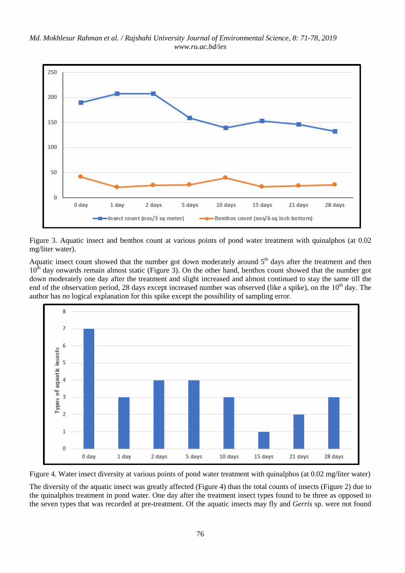
Md. Mokhlesur Rahman et al. / Rajshahi University Journal of Environmental Science, 8: 71-78, 2019 www.ru.ac.bd/ies
76
Figure 3. Aquatic insect and benthos count at various points of pond water treatment with quinalphos (at 0.02 mg/liter water).
Aquatic insect count showed that the number got down moderately around 5th days after the treatment and then 10th day onwards remain almost static (Figure 3). On the other hand, benthos count showed that the number got down moderately one day after the treatment and slight increased and almost continued to stay the same till the end of the observation period, 28 days except increased number was observed (like a spike), on the 10th day. The author has no logical explanation for this spike except the possibility of sampling error.
Figure 4. Water insect diversity at various points of pond water treatment with quinalphos (at 0.02 mg/liter water)
The diversity of the aquatic insect was greatly affected (Figure 4) than the total counts of insects (Figure 2) due to the quinalphos treatment in pond water. One day after the treatment insect types found to be three as opposed to the seven types that was recorded at pre-treatment. Of the aquatic insects may fly and Gerris sp. were not found
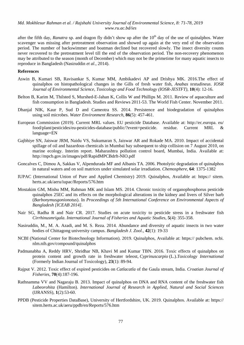
Md. Mokhlesur Rahman et al. / Rajshahi University Journal of Environmental Science, 8: 71-78, 2019 www.ru.ac.bd/ies
77
after the fifth day, Ranatra sp. and dragon fly didn’t show up after the 10th day of the use of quinalphos. Water scavenger was missing after pretreatment observation and showed up again at the very end of the observation period. The number of backswimmer and boatman declined but recovered slowly. The insect diversity counts never recovered to the pretreatment level till the end of the observation period. The non-recovery phenomenon may be attributed to the season (month of December) which may not be the primetime for many aquatic insects to reproduce in Bangladesh (Nasiruddin et al., 2014).
References
Aswin B, Kumari SB, Ravisankar S, Kumar MM, Ambikadevi AP and Drishya MK. 2016.The effect of quinalphos on histopathological changes in the Gills of fresh water fish, Anabas testudineus. IOSR Journal of Environmental Science, Toxicology and Food Technology (IOSR-JESTFT), 10(4): 12-16.
Belton B, Karim M, Thilsted S, Murshed-E-Jahan K, Collis W and Phillips M. 2011. Review of aquaculture and fish consumption in Bangladesh. Studies and Reviews 2011-53. The World Fish Center. November 2011.
Dhanjal NIK, Kaur P, Sud D and Cameotra SS. 2014. Persistence and biodegradation of quinalphos using soil microbes. Water Environment Research, 86(5): 457-461.
European Commission (2019). Current MRL values. EU pesticide Database. Available at: http://ec.europa. eu/ food/plant/pesticides/eu-pesticides-database/public/?event=pesticide. residue. Current MRL & language=EN
Gajbhiye SN, Jaiswar JRM, Naidu VS, Sukumaran S, Jaiswar AR and Rokade MA. 2010. Impact of accidental spillage of oil and hazardous chemicals in Mumbai bay subsequent to ship collision on 7 August 2010, on marine ecology. Interim report. Maharashtra pollution control board, Mumbai, India. Available at: http://mpcb.gov.in/images/pdf/RapidMPCBdrft-NIO.pdf
Goncalves C, Dimou A, Sakkas V, Alpendurada MF and Albanis TA. 2006. Photolytic degradation of quinalphos in natural waters and on soil matrices under simulated solar irradiation. Chemosphere, 64: 1375-1382
IUPAC (International Union of Pure and Applied Chemistry) 2019. Quinalphos, Available at: https:// sitem. herts.ac.uk/aeru/iupac/Reports/576.htm
Mostakim GM, Mishu MM, Rahman MK and Islam MS. 2014. Chronic toxicity of organophosphorus pesticide quinalphos 25EC and its effects on the morphological alterations in the kidney and livers of Silver barb (Barbonymusgonionotus). In Proceedings of 5th International Conference on Environmental Aspects of Bangladesh [ICEAB 2014].
Nair SG, Radha R and Nair CR. 2017. Studies on acute toxicity to pesticide stress in a freshwater fish Cirrhinusmrigala. International Journal of Fisheries and Aquatic Studies, 5(4): 355-358.
Nasiruddin, M., M. A. Azadi, and M. S. Reza. 2014. Abundance and diversity of aquatic insects in two water bodies of Chittagong university campus. Bangladesh J. Zool., 42(1): 19-33
NCBI (National Center for Biotechnology Information). 2019. Quinalphos, Available at: https:// pubchem. ncbi. nlm.nih.gov/compound/quinalphos
Padmanabha A, Reddy HRV, Shridhar NB, Khavi M and Kumar TBN. 2016. Toxic effects of quinalphos on protein content and growth rate in freshwater teleost, Cyprinuscarpio (L.).Toxicology International (Formerly Indian Journal of Toxicology), 23(1): 89-94.
Rajput V. 2012. Toxic effect of expired pesticides on Catlacatla of the Gaula stream, India. Croatian Journal of Fisheries, 70(4):187-196.
Rathnamma VV and Nagaraju B. 2013. Impact of quinalphos on DNA and RNA content of the freshwater fish Labeorohita (Hamilton). International Journal of Research in Applied, Natural and Social Sciences (IJRANSS), 1(2):53-60.
PPDB (Pesticide Properties DataBase), University of Hertfordshire, UK. 2019. Quinalphos. Available at: https:// sitem.herts.ac.uk/aeru/ppdb/en/Reports/576.htm
Md. Mokhlesur Rahman et al. / Rajshahi University Journal of Environmental Science, 8: 71-78, 2019 www.ru.ac.bd/ies
78
Siddiqui KU, Islam MA, Kabir SMH, Ahmad M, Ahmed ATA, Rahman AKA, Haque EU, Ahmed ZU, Begum ZNT, Hassa MA, Khondker M and Rahman MM (eds.). 2007. Encyclopedia of Flora and Fauna of Bangladesh, Vol. 23. Freshwater Fisher. Asiatic Society of Bangladesh, Dhaka. 300p.
Talwar MP, Mulla SI and Ninnekar HZ. 2014. Biodegradation of organophosphate pesticide quinalphos by Ochrobactrum sp. strain HZM. Journal of Applied Microbiology, 117: 1283-1292. doi: 10. 1111/ jam. 12627
Thinh NQ, Phu TM, Douny C, Phuong NT, Huong DTT, Kestemont P and Scippo ML. 2018. Bioconcentration and half-life of quinalphos pesticide in rice-fish integration system in the Mekong Delta, Vietnam. Journal of Environmental Science and Health, 53(1): 35-41.
Wahab MA. 2003. Small indigenous fish species of Bangladesh: potentials for culture and conservation,In: (Wahab MA, Thilsted SH, and Hoq ME; eds.):Small indigenous species of fish in Bangladesh: culture potentials for improved nutrition &livelihood. Bangladesh Agricultural University, Mymensingh, Bangladesh, 1-12.
Welch PS. 1948. Limnological Methods, McGraw Hill Book Company, New York. 381p.
Mst. Shifat Rumana / Rajshahi University Journal of Environmental Science, 8: 79-92, 2019 www.ru.ac.bd/ies
Adaptation Strategies of GOs and NGOs for Flood Management in the Teesta Floodplain Area in Rangpur District of Bangladesh
Mst. Shifat Rumana∗
Department of Geography and Environmental Science, Begum Rokeya University, Rangpur, Bangladesh
Abstract
In the Teesta river basin area, people suffer and fight against flood almost every year. Flood affected people get support from GOs, NGOs and other private organizations in pre, during and post flooding period. But these supports are not sufficient for them and they fall in long term poverty trap which refers to the incapability of achieving a minimum standard of living. So this study presents various adaptation strategies of GOs and NGOs, and suggests some recommendations to rapid recover from flood disaster in the research area. The study area is located in flood prone region of the Teesta river basin in Rangpur district of Bangladesh. Lakshmitari union of Gangachara upazila and Kaunia Balapara union of Kaunia upazila have been selected for this study. Primary and secondary data have been collected to fulfill the research objectives. The research findings indicate that flood is occurred every year in the study area. To minimize the damages of flood, GOs and NGOs take various steps. These steps awareness build-up of people, building embankment and shelter center, operate rescue operation, giving relief and emergency treatment, etc. But these activities are not sufficient fully to reduce the impacts of flood. So this study recommends some policies like building embankment in total eroded area, develop early warning system, increase the number of flood shelter center, etc. to minimize the damage of flood and improve the life standard of flood affected people in the study area.
Keywords: Flood; Adaptation Strategies; GOs; NGOs; Teesta Floodplain.
1. Introduction
Bangladesh lies approximately between 20°30' and 26°40' north latitude and 88°03' and 92°40' east longitude. It is one of the biggest active deltas in the world with an area about 147570 sq. km. The country is under sub-tropical monsoon climate, annual average precipitation is 2300 mm, varying from 1200 mm in the north-west to over 5000 mm in the north-east. India borders the country in west, north and most part of east. The Bay of Bengal is in the south, Myanmar borders part of the south-eastern area. It has 405 rivers including 57 transboundary rivers, among them 54 originated from India (BWDB, 2011). Since Bangladesh achieved independence in 1971, GDP has more than tripled in real terms, food protection has increased three fold, the population growth rate has declined from around 2.9% per annum in 1974 to 1.4% in 2006 and the country is largely food secure. Over the last 20 years, growth has accelerated and the country is on track to become a middle income country by 2021 when it will celebrate its 50 years of independence (MoEF, 2009). Despite these successes, the country is highly vulnerable to natural hazards like catastrophic cyclones, tornadoes, storm surges, droughts, floods, earthquakes, riverbank erosion, and landslides. Floods are the most common natural hazard affecting Bangladesh, with about 20 million people present in zones subject to flooding (Gemenne et al., 2011). Bangladesh is mostly flat except some hilly part in the southeast and the northeast and about all rivers are come in our country in mature stage. This country was formed due to sedimentation of the large river systems. For these reason some 30 to 35% of the total land surface of the country is flooded every year during wet monsoon (Milliman et al., 1989). Flooding is one such water related environmental problem magnitude of which is very much dependent on land-use practices in the watershed of each rivers or streams (Khalequzzaman, 2000).
According to Nishat, 2004, an area goes under and remains under water for some times, it is inundation. When inundation causes damage to property and crops, disrupts communication and brings harmful effects to human beings as well as flora and fauna, we call it flood. So it is said that inundation and damage are together considered as flood.
When water flow of the river or other channel exceeds certain stage, spreads the bank area or adjoining high land and damages the environment and man-made things this situation is enumerated as flood (Rumana, 2020).
∗ Corresponding author’s e-mail: [email protected]
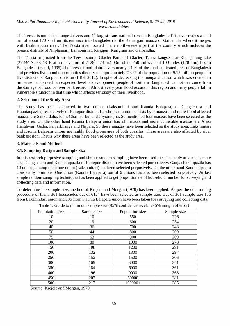
Mst. Shifat Rumana / Rajshahi University Journal of Environmental Science, 8: 79-92, 2019 www.ru.ac.bd/ies
80
The Teesta is one of the longest rivers and 4th largest trans-national river in Bangladesh. This river makes a total run of about 170 km from its entrance into Bangladesh to the Kamargani mauza of Gaibandha where it merges with Brahmaputra river. The Teesta river located in the north-western part of the country which includes the present districts of Nilphamari, Lalmonirhat, Rangpur, Kurigram and Gaibandha.
The Teesta originated from the Teesta source Glacier-Pauhunri Glacier, Teesta kangse near Khangchung lake (27°59' N; 38°48' E at an elevation of 7128©/2173 m.). Out of its 250 miles about 100 miles (170 km.) lies in Bangladesh (Hanif, 1995).The Teesta flood plain covers nearly 14 % of the total cultivated area of Bangladesh and provides livelihood opportunities directly to approximately 7.3 % of the population or 9.15 million people in five districts of Rangpur division (BBS, 2012). In spite of decreasing the monga situation which was created an immense bar to reach an expected level of development, people of northern Bangladesh cannot overcome from the damage of flood or river bank erosion. Almost every year flood occurs in this region and many people fall in vulnerable situation in that time which affects seriously on their livelihood.
2. Selection of the Study Area
The study has been conducted in two unions (Lakshmitari and Kaunia Balapara) of Gangachara and Kauniaupazila, respectively of Rangpur district. Lakshmitari union consists by 9 mauzas and more flood affected mauzas are Sankardaha, Ichli, Char Isorkul and Joyramojha. So mentioned four mauzas have been selected as the study area. On the other hand Kaunia Balapara union has 21 mauzas and more vulnerable mauzas are Arazi Harishwar, Gadai, Panjarbhanga and Nijpara. So these mauzas have been selected as the study area. Lakshmitari and Kaunia Balapara unions are highly flood prone area of both upazilas. These areas are also affected by river bank erosion. That is why these areas have been selected as the study area.
3. Materials and Method
3.1. Sampling Design and Sample Size
In this research purposive sampling and simple random sampling have been used to select study area and sample size. Gangachara and Kaunia upazila of Rangpur district have been selected purposively. Gangachara upazila has 10 unions, among them one union (Lakshmitari) has been selected purposively. On the other hand Kaunia upazila consists by 6 unions. One union (Kaunia Balapara) out of 6 unions has also been selected purposively. At last simple random sampling techniques has been applied to get proportionate of household number for surveying and collecting data and information.
To determine the sample size, method of Krejcie and Morgan (1970) has been applied. As per the determining procedure of them, 361 households out of 6124 have been selected as sample size. Out of 361 sample size 156 from Lakshmitari union and 205 from Kaunia Balapara union have been taken for surveying and collecting data. Table 1. Guide to minimum sample size (95% confidence level, +/- 5% margin of error)
Population size Sample size Population size Sample size 10 10 550 226 20 19 600 234 40 36 700 248 50 44 800 260 75 63 900 269
100 80 1000 278 150 108 1200 291 200 132 1300 297 250 152 1500 306 300 169 3000 341 350 184 6000 361 400 196 9000 368 450 207 50000 381 500 217 100000+ 385
Source: Krejcie and Morgan, 1970
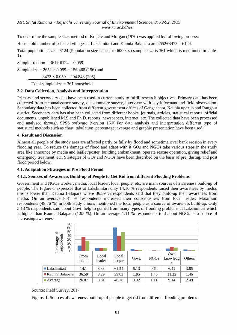
Mst. Shifat Rumana / Rajshahi University Journal of Environmental Science, 8: 79-92, 2019 www.ru.ac.bd/ies
81
Frommedia
Localleader
Localpeople Govt. NGOs
Ownknowledg
eOthers
Lakshmitari 14.1 8.33 61.54 5.13 0.64 6.41 3.85Kaunia Balapara 36.59 8.29 39.03 1.95 1.46 11.22 1.46Average 26.87 8.31 48.76 3.32 1.11 9.14 2.49
010203040506070
Perc
enta
ge o
f re
spon
dent
s
To determine the sample size, method of Krejcie and Morgan (1970) was applied by following process: Household number of selected villages at Lakshmitari and Kaunia Balapara are 2652+3472 = 6124. Total population size = 6124 (Population size is near to 6000, so sample size is 361 which is mentioned in table-1). Sample fraction = 361÷ 6124 = 0.059 Sample size = 2652 × 0.059 = 156.468 (156) and 3472 × 0.059 = 204.848 (205)
Total sample size = 361 household 3.2. Data Collection, Analysis and Interpretation Primary and secondary data have been used in current study to fulfill research objectives. Primary data has been collected from reconnaissance survey, questionnaire survey, interview with key informant and field observation. Secondary data has been collected from different government offices of Gangachara, Kaunia upazila and Rangpur district. Secondary data has also been collected from different books, journals, articles, statistical reports, official documents, unpublished M.S and Ph.D. reports, newspapers, internet, etc. The collected data have been processed and analyzed through SPSS software (version 16.0).For data analysis and interpretation different type of statistical methods such as chart, tabulation, percentage, average and graphic presentation have been used. 4. Result and Discussion Almost all people of the study area are affected partly or fully by flood and sometime river bank erosion in every flooding year. To reduce the damage of flood and adapt with it GOs and NGOs take various steps in the study area like announce by media and leaflet/poster, building embankment, operate rescue operation, giving relief and emergency treatment, etc. Strategies of GOs and NGOs have been described on the basis of pre, during, and post flood period below. 4.1. Adaptation Strategies in Pre Flood Period 4.1.1. Sources of Awareness Build-up of People to Get Rid from different Flooding Problems Government and NGOs worker, media, local leader, local people, etc. are main sources of awareness build-up of people. The Figure-1 expresses that at Lakshmitari only 14.10 % respondents raised their awareness by media, this is lower than Kaunia Balapara where 36.59 % respondents said that they build-up their awareness from media. On an average 8.31 % respondents increased their consciousness from local leader. Maximum respondents (48.76 %) in both study unions mentioned the local people as a source of awareness build-up. Only 5.13 % respondents said about Govt. help to get rid from many types of flooding problems at Lakshmitari which is higher than Kaunia Balapara (1.95 %). On an average 1.11 % respondents told about NGOs as a source of increasing awareness.
Source: Field Survey, 2017
Figure: 1. Sources of awareness build-up of people to get rid from different flooding problems
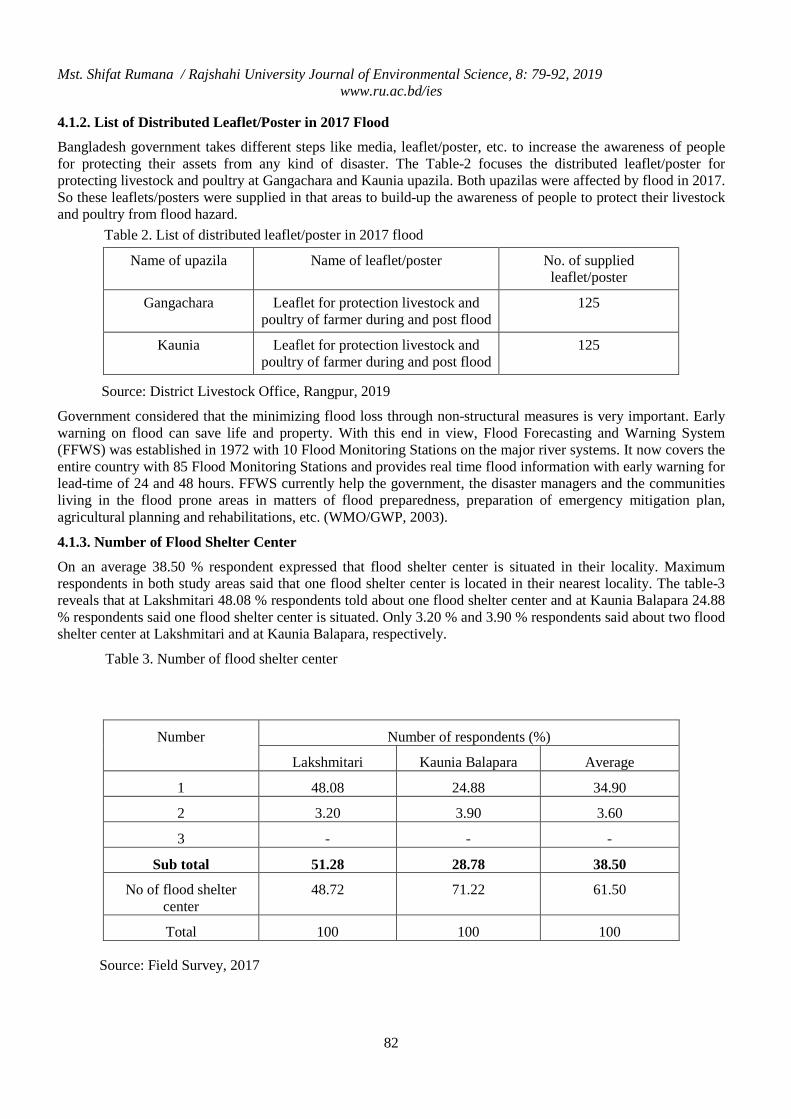
Mst. Shifat Rumana / Rajshahi University Journal of Environmental Science, 8: 79-92, 2019 www.ru.ac.bd/ies
82
4.1.2. List of Distributed Leaflet/Poster in 2017 Flood
Bangladesh government takes different steps like media, leaflet/poster, etc. to increase the awareness of people for protecting their assets from any kind of disaster. The Table-2 focuses the distributed leaflet/poster for protecting livestock and poultry at Gangachara and Kaunia upazila. Both upazilas were affected by flood in 2017. So these leaflets/posters were supplied in that areas to build-up the awareness of people to protect their livestock and poultry from flood hazard.
Table 2. List of distributed leaflet/poster in 2017 flood
Name of upazila Name of leaflet/poster No. of supplied leaflet/poster
Gangachara Leaflet for protection livestock and poultry of farmer during and post flood
125
Kaunia Leaflet for protection livestock and poultry of farmer during and post flood
125
Source: District Livestock Office, Rangpur, 2019
Government considered that the minimizing flood loss through non-structural measures is very important. Early warning on flood can save life and property. With this end in view, Flood Forecasting and Warning System (FFWS) was established in 1972 with 10 Flood Monitoring Stations on the major river systems. It now covers the entire country with 85 Flood Monitoring Stations and provides real time flood information with early warning for lead-time of 24 and 48 hours. FFWS currently help the government, the disaster managers and the communities living in the flood prone areas in matters of flood preparedness, preparation of emergency mitigation plan, agricultural planning and rehabilitations, etc. (WMO/GWP, 2003).
4.1.3. Number of Flood Shelter Center
On an average 38.50 % respondent expressed that flood shelter center is situated in their locality. Maximum respondents in both study areas said that one flood shelter center is located in their nearest locality. The table-3 reveals that at Lakshmitari 48.08 % respondents told about one flood shelter center and at Kaunia Balapara 24.88 % respondents said one flood shelter center is situated. Only 3.20 % and 3.90 % respondents said about two flood shelter center at Lakshmitari and at Kaunia Balapara, respectively.
Table 3. Number of flood shelter center
Source: Field Survey, 2017
Number Number of respondents (%)
Lakshmitari Kaunia Balapara Average
1 48.08 24.88 34.90
2 3.20 3.90 3.60
3 - - -
Sub total 51.28 28.78 38.50
No of flood shelter center
48.72 71.22 61.50
Total 100 100 100
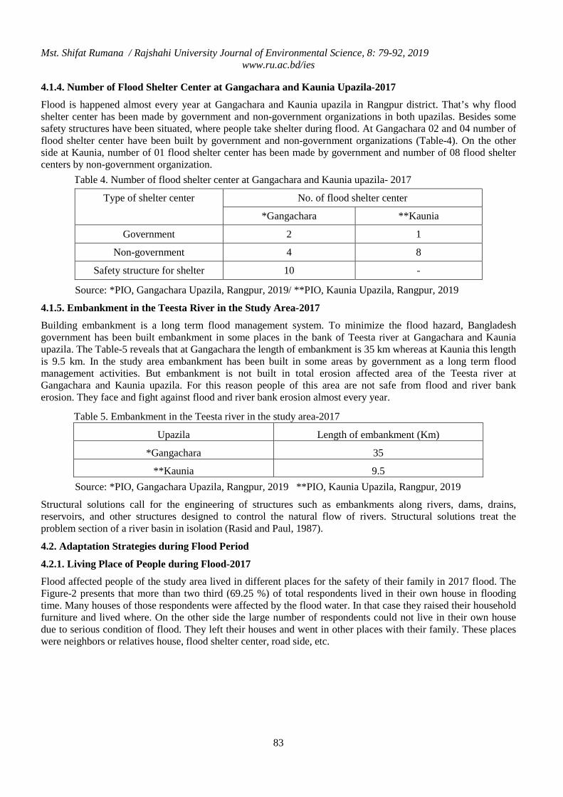
Mst. Shifat Rumana / Rajshahi University Journal of Environmental Science, 8: 79-92, 2019 www.ru.ac.bd/ies
83
4.1.4. Number of Flood Shelter Center at Gangachara and Kaunia Upazila-2017
Flood is happened almost every year at Gangachara and Kaunia upazila in Rangpur district. That’s why flood shelter center has been made by government and non-government organizations in both upazilas. Besides some safety structures have been situated, where people take shelter during flood. At Gangachara 02 and 04 number of flood shelter center have been built by government and non-government organizations (Table-4). On the other side at Kaunia, number of 01 flood shelter center has been made by government and number of 08 flood shelter centers by non-government organization.
Source: *PIO, Gangachara Upazila, Rangpur, 2019/ **PIO, Kaunia Upazila, Rangpur, 2019
4.1.5. Embankment in the Teesta River in the Study Area-2017
Building embankment is a long term flood management system. To minimize the flood hazard, Bangladesh government has been built embankment in some places in the bank of Teesta river at Gangachara and Kaunia upazila. The Table-5 reveals that at Gangachara the length of embankment is 35 km whereas at Kaunia this length is 9.5 km. In the study area embankment has been built in some areas by government as a long term flood management activities. But embankment is not built in total erosion affected area of the Teesta river at Gangachara and Kaunia upazila. For this reason people of this area are not safe from flood and river bank erosion. They face and fight against flood and river bank erosion almost every year.
Source: *PIO, Gangachara Upazila, Rangpur, 2019 **PIO, Kaunia Upazila, Rangpur, 2019
Structural solutions call for the engineering of structures such as embankments along rivers, dams, drains, reservoirs, and other structures designed to control the natural flow of rivers. Structural solutions treat the problem section of a river basin in isolation (Rasid and Paul, 1987).
4.2. Adaptation Strategies during Flood Period
4.2.1. Living Place of People during Flood-2017
Flood affected people of the study area lived in different places for the safety of their family in 2017 flood. The Figure-2 presents that more than two third (69.25 %) of total respondents lived in their own house in flooding time. Many houses of those respondents were affected by the flood water. In that case they raised their household furniture and lived where. On the other side the large number of respondents could not live in their own house due to serious condition of flood. They left their houses and went in other places with their family. These places were neighbors or relatives house, flood shelter center, road side, etc.
Table 4. Number of flood shelter center at Gangachara and Kaunia upazila- 2017
Type of shelter center No. of flood shelter center
*Gangachara **Kaunia
Government 2 1
Non-government 4 8
Safety structure for shelter 10 -
Table 5. Embankment in the Teesta river in the study area-2017
Upazila Length of embankment (Km)
*Gangachara 35
**Kaunia 9.5
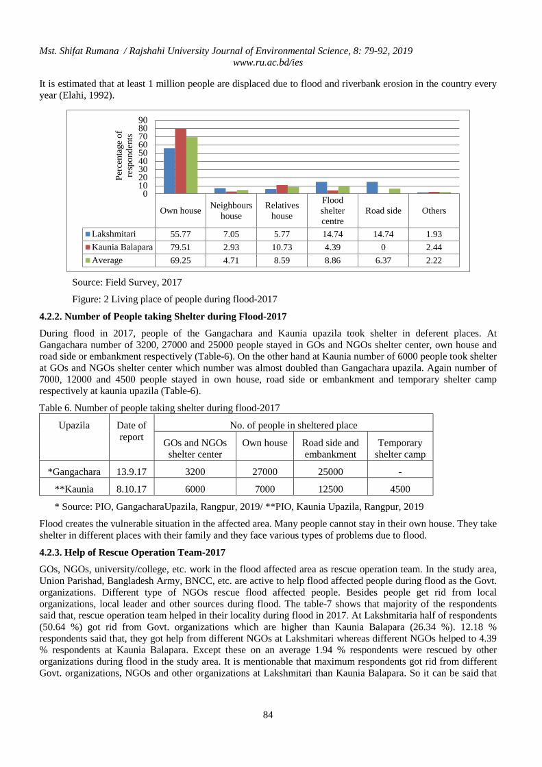
Mst. Shifat Rumana / Rajshahi University Journal of Environmental Science, 8: 79-92, 2019 www.ru.ac.bd/ies
84
Own house Neighbourshouse
Relativeshouse
Floodsheltercentre
Road side Others
Lakshmitari 55.77 7.05 5.77 14.74 14.74 1.93Kaunia Balapara 79.51 2.93 10.73 4.39 0 2.44Average 69.25 4.71 8.59 8.86 6.37 2.22
0102030405060708090
Perc
enta
ge o
f re
spon
dent
s
It is estimated that at least 1 million people are displaced due to flood and riverbank erosion in the country every year (Elahi, 1992).
Source: Field Survey, 2017
Figure: 2 Living place of people during flood-2017
4.2.2. Number of People taking Shelter during Flood-2017
During flood in 2017, people of the Gangachara and Kaunia upazila took shelter in deferent places. At Gangachara number of 3200, 27000 and 25000 people stayed in GOs and NGOs shelter center, own house and road side or embankment respectively (Table-6). On the other hand at Kaunia number of 6000 people took shelter at GOs and NGOs shelter center which number was almost doubled than Gangachara upazila. Again number of 7000, 12000 and 4500 people stayed in own house, road side or embankment and temporary shelter camp respectively at kaunia upazila (Table-6).
Table 6. Number of people taking shelter during flood-2017
Upazila Date of report
No. of people in sheltered place
GOs and NGOs shelter center
Own house Road side and embankment
Temporary shelter camp
*Gangachara 13.9.17 3200 27000 25000 -
**Kaunia 8.10.17 6000 7000 12500 4500
* Source: PIO, GangacharaUpazila, Rangpur, 2019/ **PIO, Kaunia Upazila, Rangpur, 2019
Flood creates the vulnerable situation in the affected area. Many people cannot stay in their own house. They take shelter in different places with their family and they face various types of problems due to flood.
4.2.3. Help of Rescue Operation Team-2017
GOs, NGOs, university/college, etc. work in the flood affected area as rescue operation team. In the study area, Union Parishad, Bangladesh Army, BNCC, etc. are active to help flood affected people during flood as the Govt. organizations. Different type of NGOs rescue flood affected people. Besides people get rid from local organizations, local leader and other sources during flood. The table-7 shows that majority of the respondents said that, rescue operation team helped in their locality during flood in 2017. At Lakshmitaria half of respondents (50.64 %) got rid from Govt. organizations which are higher than Kaunia Balapara (26.34 %). 12.18 % respondents said that, they got help from different NGOs at Lakshmitari whereas different NGOs helped to 4.39 % respondents at Kaunia Balapara. Except these on an average 1.94 % respondents were rescued by other organizations during flood in the study area. It is mentionable that maximum respondents got rid from different Govt. organizations, NGOs and other organizations at Lakshmitari than Kaunia Balapara. So it can be said that
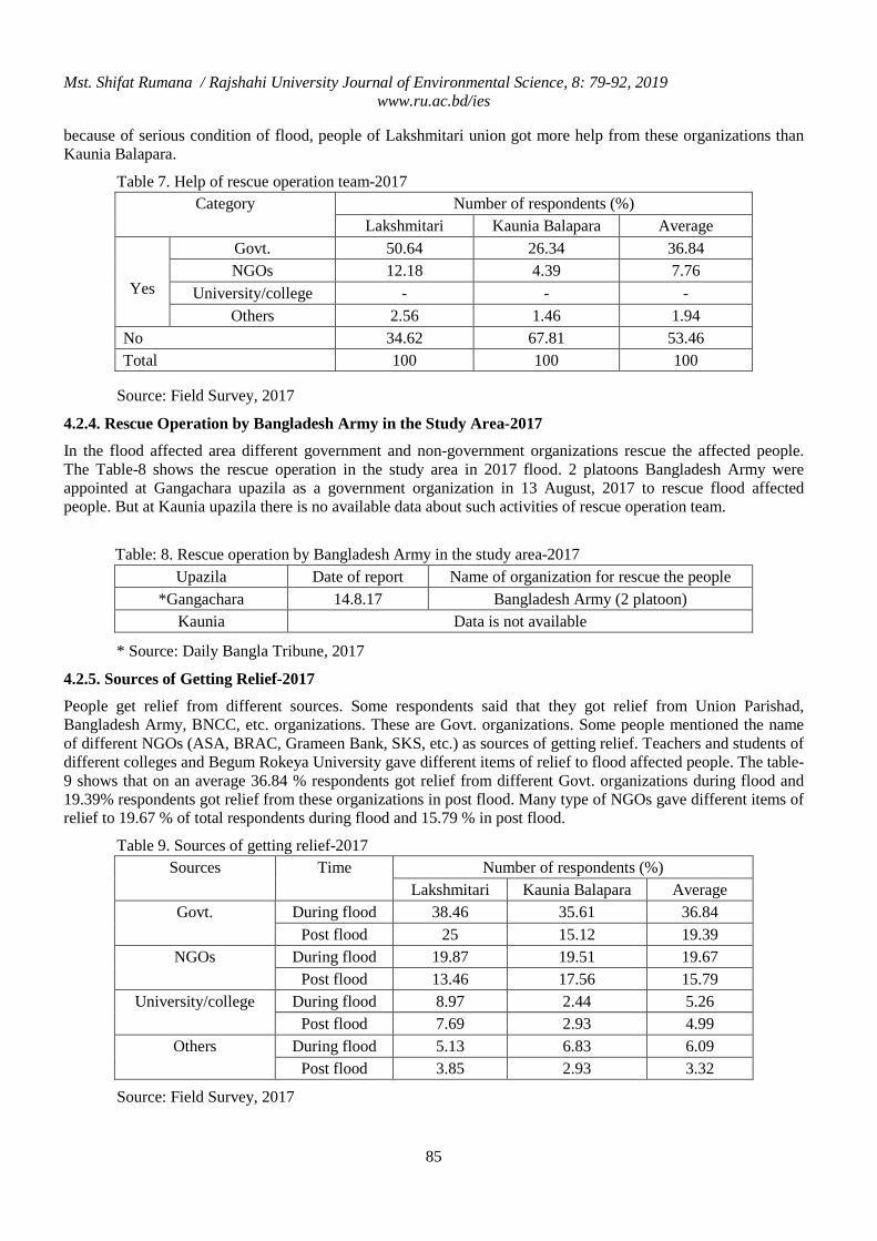
Mst. Shifat Rumana / Rajshahi University Journal of Environmental Science, 8: 79-92, 2019 www.ru.ac.bd/ies
85
because of serious condition of flood, people of Lakshmitari union got more help from these organizations than Kaunia Balapara.
Table 7. Help of rescue operation team-2017
Source: Field Survey, 2017
4.2.4. Rescue Operation by Bangladesh Army in the Study Area-2017
In the flood affected area different government and non-government organizations rescue the affected people. The Table-8 shows the rescue operation in the study area in 2017 flood. 2 platoons Bangladesh Army were appointed at Gangachara upazila as a government organization in 13 August, 2017 to rescue flood affected people. But at Kaunia upazila there is no available data about such activities of rescue operation team.
Table: 8. Rescue operation by Bangladesh Army in the study area-2017
Upazila Date of report Name of organization for rescue the people *Gangachara 14.8.17 Bangladesh Army (2 platoon)
Kaunia Data is not available
* Source: Daily Bangla Tribune, 2017
4.2.5. Sources of Getting Relief-2017
People get relief from different sources. Some respondents said that they got relief from Union Parishad, Bangladesh Army, BNCC, etc. organizations. These are Govt. organizations. Some people mentioned the name of different NGOs (ASA, BRAC, Grameen Bank, SKS, etc.) as sources of getting relief. Teachers and students of different colleges and Begum Rokeya University gave different items of relief to flood affected people. The table-9 shows that on an average 36.84 % respondents got relief from different Govt. organizations during flood and 19.39% respondents got relief from these organizations in post flood. Many type of NGOs gave different items of relief to 19.67 % of total respondents during flood and 15.79 % in post flood.
Table 9. Sources of getting relief-2017
Source: Field Survey, 2017
Category Number of respondents (%) Lakshmitari Kaunia Balapara Average
Yes
Govt. 50.64 26.34 36.84 NGOs 12.18 4.39 7.76
University/college - - - Others 2.56 1.46 1.94
No 34.62 67.81 53.46 Total 100 100 100
Sources Time Number of respondents (%) Lakshmitari Kaunia Balapara Average
Govt. During flood 38.46 35.61 36.84 Post flood 25 15.12 19.39
NGOs During flood 19.87 19.51 19.67 Post flood 13.46 17.56 15.79
University/college During flood 8.97 2.44 5.26 Post flood 7.69 2.93 4.99
Others During flood 5.13 6.83 6.09 Post flood 3.85 2.93 3.32
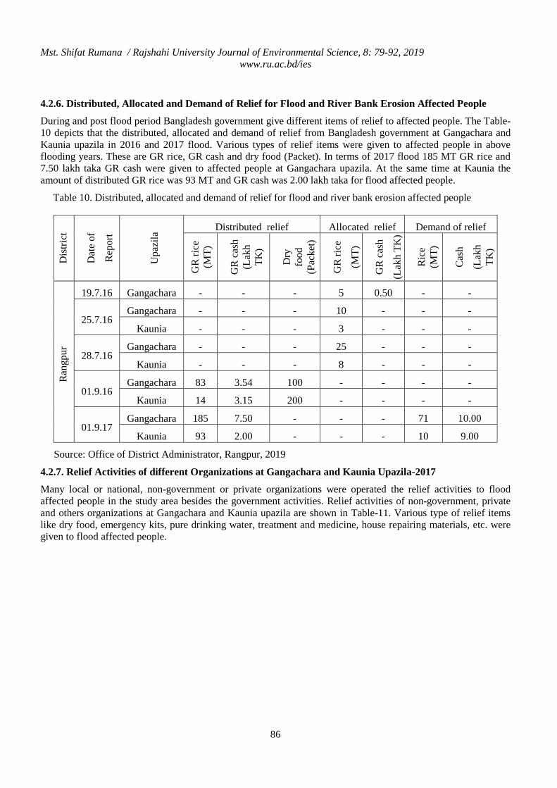
Mst. Shifat Rumana / Rajshahi University Journal of Environmental Science, 8: 79-92, 2019 www.ru.ac.bd/ies
86
4.2.6. Distributed, Allocated and Demand of Relief for Flood and River Bank Erosion Affected People
During and post flood period Bangladesh government give different items of relief to affected people. The Table-10 depicts that the distributed, allocated and demand of relief from Bangladesh government at Gangachara and Kaunia upazila in 2016 and 2017 flood. Various types of relief items were given to affected people in above flooding years. These are GR rice, GR cash and dry food (Packet). In terms of 2017 flood 185 MT GR rice and 7.50 lakh taka GR cash were given to affected people at Gangachara upazila. At the same time at Kaunia the amount of distributed GR rice was 93 MT and GR cash was 2.00 lakh taka for flood affected people.
Table 10. Distributed, allocated and demand of relief for flood and river bank erosion affected people
4.2.7. Relief Activities of different Organizations at Gangachara and Kaunia Upazila-2017
Many local or national, non-government or private organizations were operated the relief activities to flood affected people in the study area besides the government activities. Relief activities of non-government, private and others organizations at Gangachara and Kaunia upazila are shown in Table-11. Various type of relief items like dry food, emergency kits, pure drinking water, treatment and medicine, house repairing materials, etc. were given to flood affected people.
Dis
trict
Dat
e of
Rep
ort
Upa
zila
Distributed relief Allocated relief Demand of relief
GR
rice
(M
T)
GR
cas
h (L
akh
TK)
Dry
fo
od
(Pac
ket)
GR
rice
(MT)
GR
cas
h
(Lak
h TK
)
Ric
e (M
T)
Cas
h
(Lak
h TK
)
Ran
gpur
19.7.16 Gangachara - - - 5 0.50 - -
25.7.16 Gangachara - - - 10 - - -
Kaunia - - - 3 - - -
28.7.16 Gangachara - - - 25 - - -
Kaunia - - - 8 - - -
01.9.16 Gangachara 83 3.54 100 - - - -
Kaunia 14 3.15 200 - - - -
01.9.17 Gangachara 185 7.50 - - - 71 10.00
Kaunia 93 2.00 - - - 10 9.00
Source: Office of District Administrator, Rangpur, 2019
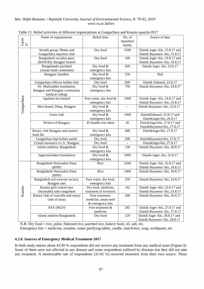
Mst. Shifat Rumana / Rajshahi University Journal of Environmental Science, 8: 79-92, 2019 www.ru.ac.bd/ies
87
Table 11. Relief activities of different organizations at Gangachara and Kaunia upazila-2017
Upa
zila
Name of organizations Relief item No. of benefited
family
Source of data
Gan
gach
ara
Wealth group, Dhaka and Gangachara reporters club
Dry food 3500 Dainik Juger Alo, 15.8.17 and Dainik Bayannor Alo, 15.8.17
Bangladesh socialist party (BASOD), Rangpur branch
Dry food 100 Dainik Juger Alo, 19.8.17 and Dainik Bayannor Alo, 19.8.17
Bangabandu parishad (Janata bank committee)
Dry food & emergency kits
420 Dainik Juger Alo, 23.8.17
Rangpur chamber Dry food & emergency kits
250 Ibid
Gangachara officers kollan club Dry food 600 Dainik Dabanol, 23.8.17 Dr. Mafizuddin foundation,
Rangpur and Rangpur community medical college
Dry food & emergency kits
750 Dainik Bayannor Alo, 24.8.17
Ispahani tea limited Pure water, dry food & emergency kits
1000 Dainik Juger Alo, 24.8.17 and Dainik Bayannor Alo, 25.8.17
Mou hostel, Dhap, Rangpur Dry food & emergency kits
- Dainik Bayannor Alo, 25.8.17
Lions club Dry food & emergency kits
1000 DainikDabanol, 25.8.17 and DainikJugerAlo, 26.8.17
Writers of Rangpur 45 bundle iron sheet 45 DainikJugerAlo, 27.8.17 and DainikBayannorAlo, 27.8.17
Rotary club Rangpur and eastern bank ltd.
Dry food & emergency kits
400 DainikJugerAlo, 27.8.17
Gangachara haji kollan samiti Dry food 200 DainikBayannorAlo, 27.8.17 Cristal insurance co. li., Rangpur Dry food - DainikJugerAlo, 27.8.17
Islami andolon, Bangladesh Dry food & emergency kits
130 Dainik Bayannor Alo, 28.8.17
Jagoronichakro foundation Dry food & emergency kits
1000 Dainik Juger Alo, 31.8.17
Kau
nia
Bangladesh Nationalist Party (BNP)
Rice 2500 Dainik Juger Alo, 16.8.17 and Dainik Bayannor Alo, 16.8.17
Bangladesh Nationalist Party (BNP)
Rice 1400 Dainik Bayannor Alo, 19.8.17
Bangladesh red crescent society, Rangpur unit
Pure water, dry food, emergency kits
250 Dainik Bayannor Alo, 24.8.17
Kaunia girls school mor choymatha zubo sangothon
Dry food, medicine, treatment of livestock
162 Dainik Juger Alo, 25.8.17 and Dainik Bayannor Alo, 25.8.17
Rotary club of roseville and rotary club of uttara
Free treatment, medicine, aman seed
& emergency kits
500 Dainik Bayannor Alo, 26.8.17
ASA (NGO) Free treatment & medicine
285 Dainik Juger Alo, 27.8.17 and Dainik Bayannor Alo, 27.8.17
Islami andolon Bangladesh Dry food 120 Dainik Juger Alo, 28.8.17 and Dainik Bayannor Alo, 28.8.17
N.B: Dry food = rice, pulse, flattened rice, parched rice, bakery food, oil, salt, etc. Emergency kits = medicine, orsaline, water purifying tablet, candle, match-box, soap, toothpaste, etc.
4.2.8. Sources of Emergency Medical Treatment-2017
In both study unions about 43.49 % respondents did not receive any treatment from any medical team (Figure-3). Some of them were not affected in any disease and some respondents suffered by diseases but they did not take any treatment. A mentionable rate of respondents (31.03 %) received treatment from their own source. These

Mst. Shifat Rumana / Rajshahi University Journal of Environmental Science, 8: 79-92, 2019 www.ru.ac.bd/ies
88
No treatment Govt. NGOs Socialcommunity Own source Others
Lakshmitari 44.23 16.67 7.05 1.92 27.57 2.56Kaunia Balapara 42.92 11.71 4.39 0 33.66 7.32Average 43.49 13.85 5.54 0.83 31.03 5.26
01020304050
Perc
enta
ge o
f re
spon
dent
s
sources were medicine store, Quack, Homeopathy, Kobiraji, etc. On the other hand on an average 13.85 % respondents got emergency medical treatment from Govt. medical team. Treatments from Bangladesh Army, village community clinic, medical team from upazila health complex, etc. are included as Govt. medical team. In both study areas 5.54 % of total respondents said that they got treatment from different NGOs in free of cost during and post flood period in 2017.
Source: Field Survey, 2017
Figure: 3. Sources of emergency medical treatment-2017
4.2.9. Activities of Emergency Medical Team in the Study Area-2017
The Table-12 provides information about activities of emergency medical team in the flooding period of 2017. Different type of non-government organizations gave emergency medical service besides the government to flood affected people and livestock in the study area.
Table 12. Activities of emergency medical team in the study area-2017
Upa
zila
Name of organizations
Trea
tmen
t fo
r hum
an/
lives
tock
No.
of
bene
fited
fa
mily
Source of data
Gan
gach
ara
Upazila Health Complex
(Medical team for all unions)
Human - Upazila Health Complex, Gangachara, Rangpur,
2019
Kau
nia
Kaunia girls school mor choymatha zubo sangothon
Livestock
162 Dainik Juger Alo, 25.8.17 & Dainik Bayannor Alo,
25.8.17
Rotary club of roseville and rotary club of uttara
Human 500 Dainik Bayannor Alo, 26.8.17
ASA (NGO) Human 285 Dainik Juger Alo, 27.8.17 & Dainik Bayannor Alo,
27.8.17
4.3. Adaptation Strategies in Post Flood Period
4.3.1. Giving Loan to Flood Victims-2017
People receive loan from different sources to fulfill their different purposes. On an average 47.65 % respondents did not receive loan after flood of 2017. Different NGOs such as Grammen Bank, BRAC, ASA, etc. gave loan to 29.64 % of total respondents. People invest their loan money in agriculture sector, business, buying domestic animal or van, rickshaw, etc. These are productive sectors. But some people use this taka in non-productive
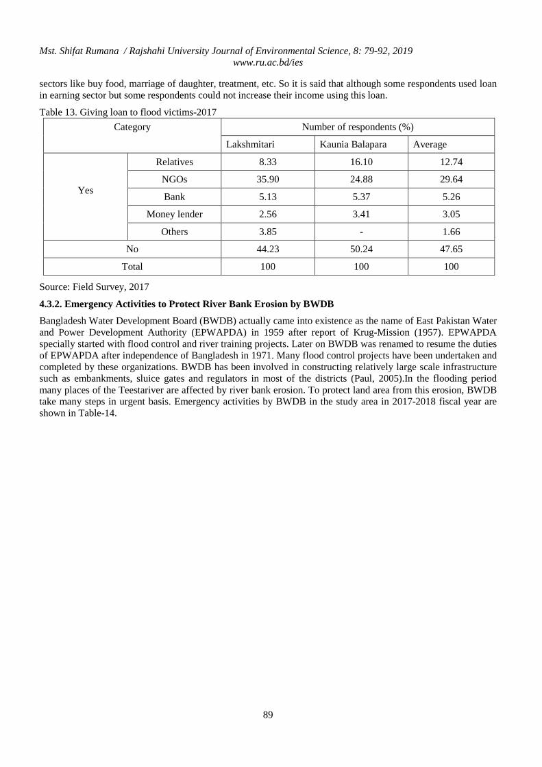
Mst. Shifat Rumana / Rajshahi University Journal of Environmental Science, 8: 79-92, 2019 www.ru.ac.bd/ies
89
sectors like buy food, marriage of daughter, treatment, etc. So it is said that although some respondents used loan in earning sector but some respondents could not increase their income using this loan.
Table 13. Giving loan to flood victims-2017 Category Number of respondents (%)
Lakshmitari Kaunia Balapara Average
Yes
Relatives 8.33 16.10 12.74
NGOs 35.90 24.88 29.64
Bank 5.13 5.37 5.26
Money lender 2.56 3.41 3.05
Others 3.85 - 1.66
No 44.23 50.24 47.65
Total 100 100 100
Source: Field Survey, 2017
4.3.2. Emergency Activities to Protect River Bank Erosion by BWDB
Bangladesh Water Development Board (BWDB) actually came into existence as the name of East Pakistan Water and Power Development Authority (EPWAPDA) in 1959 after report of Krug-Mission (1957). EPWAPDA specially started with flood control and river training projects. Later on BWDB was renamed to resume the duties of EPWAPDA after independence of Bangladesh in 1971. Many flood control projects have been undertaken and completed by these organizations. BWDB has been involved in constructing relatively large scale infrastructure such as embankments, sluice gates and regulators in most of the districts (Paul, 2005).In the flooding period many places of the Teestariver are affected by river bank erosion. To protect land area from this erosion, BWDB take many steps in urgent basis. Emergency activities by BWDB in the study area in 2017-2018 fiscal year are shown in Table-14.
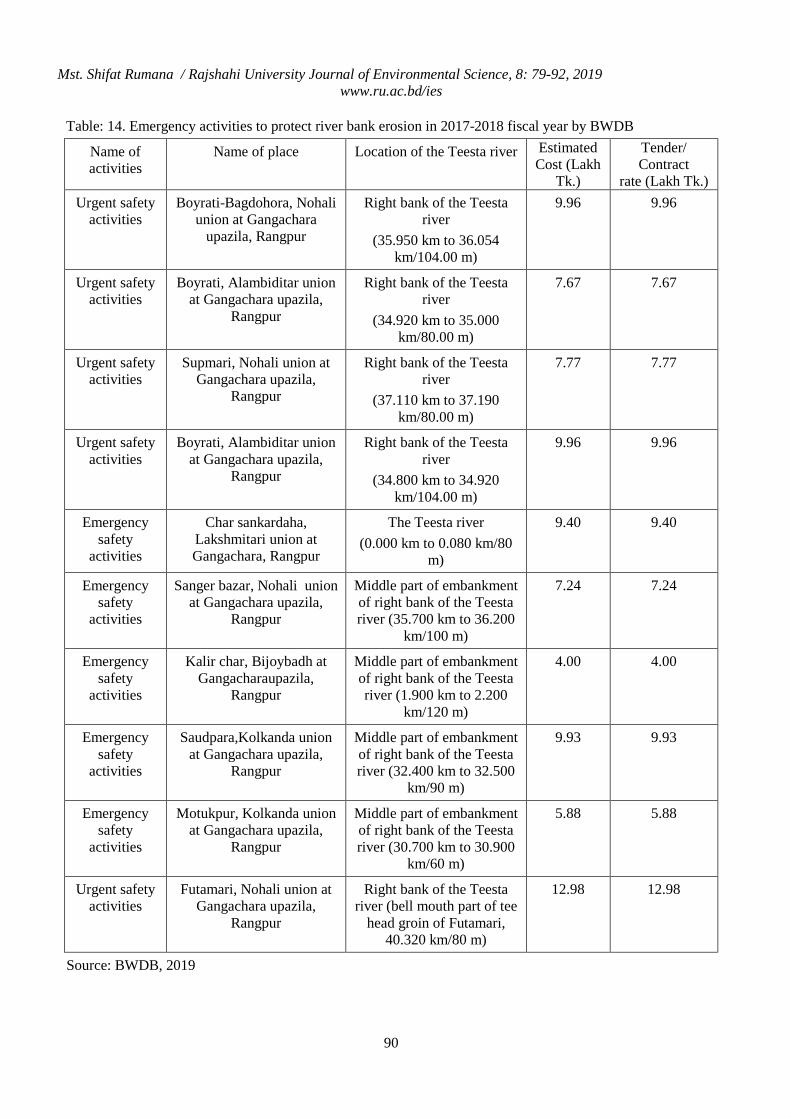
Mst. Shifat Rumana / Rajshahi University Journal of Environmental Science, 8: 79-92, 2019 www.ru.ac.bd/ies
90
Table: 14. Emergency activities to protect river bank erosion in 2017-2018 fiscal year by BWDB
Name of activities
Name of place Location of the Teesta river Estimated Cost (Lakh
Tk.)
Tender/ Contract
rate (Lakh Tk.) Urgent safety
activities Boyrati-Bagdohora, Nohali
union at Gangachara upazila, Rangpur
Right bank of the Teesta river
(35.950 km to 36.054 km/104.00 m)
9.96 9.96
Urgent safety activities
Boyrati, Alambiditar union at Gangachara upazila,
Rangpur
Right bank of the Teesta river
(34.920 km to 35.000 km/80.00 m)
7.67 7.67
Urgent safety activities
Supmari, Nohali union at Gangachara upazila,
Rangpur
Right bank of the Teesta river
(37.110 km to 37.190 km/80.00 m)
7.77 7.77
Urgent safety activities
Boyrati, Alambiditar union at Gangachara upazila,
Rangpur
Right bank of the Teesta river
(34.800 km to 34.920 km/104.00 m)
9.96 9.96
Emergency safety
activities
Char sankardaha, Lakshmitari union at Gangachara, Rangpur
The Teesta river (0.000 km to 0.080 km/80
m)
9.40 9.40
Emergency safety
activities
Sanger bazar, Nohali union at Gangachara upazila,
Rangpur
Middle part of embankment of right bank of the Teesta river (35.700 km to 36.200
km/100 m)
7.24 7.24
Emergency safety
activities
Kalir char, Bijoybadh at Gangacharaupazila,
Rangpur
Middle part of embankment of right bank of the Teesta river (1.900 km to 2.200
km/120 m)
4.00 4.00
Emergency safety
activities
Saudpara,Kolkanda union at Gangachara upazila,
Rangpur
Middle part of embankment of right bank of the Teesta river (32.400 km to 32.500
km/90 m)
9.93 9.93
Emergency safety
activities
Motukpur, Kolkanda union at Gangachara upazila,
Rangpur
Middle part of embankment of right bank of the Teesta river (30.700 km to 30.900
km/60 m)
5.88 5.88
Urgent safety activities
Futamari, Nohali union at Gangachara upazila,
Rangpur
Right bank of the Teesta river (bell mouth part of tee
head groin of Futamari, 40.320 km/80 m)
12.98 12.98
Source: BWDB, 2019
Mst. Shifat Rumana / Rajshahi University Journal of Environmental Science, 8: 79-92, 2019 www.ru.ac.bd/ies
91
5. Conclusion and Recommendations
Flood or any natural disaster cannot be stopped fully but proper management system can reduce the magnitude and destructiveness of this natural disaster. In the study area people become economically vulnerable due to flood and riverbank erosion. To recover this situation, GOs and NGOs have taken many steps and people apply their indigenous knowledge. But still now people whirl round and round in poverty trap. For a sustainable flood management in the Teesta floodplain area the study would consider the following recommendations.
• Official warning dissemination bodies have to be formed to reach the warning to rural people in proper time.
• Many flood shelter centers are need to be established, at the same time pure drinking water, proper sanitation system, emergency treatment, etc. need to be ensured in those shelters.
• Embankment should be built-up in total eroded area which can protect the villagers from flood and river bank erosion. Besides monitoring, repairing and maintenances are necessary in regular basis to sustain the embankment.
• Rescue operation, relief activates, emergency medical treatment, etc. should be applied in urgent basis and proper way.
• During and post flooding period many people are being workless. In that case more work opportunities should be created for those people. Various types of agricultural (poultry, livestock, fishery, etc.) or non-agricultural (labor, driver, shopkeeper, etc.) activities should be introduced in that area. GOs and NGOs can take necessary steps to train up people and provide logistics support like capital through soft loan.
• A master plan has to be formulated for proper land use, water and power development.
• Moreover Govt. should take proper policy, more effective plan, more in-depth studies, increase economic strength and resources to adapt with flood or any other disasters.
References
BBS. (Bangladesh Bureau of Statistics). 2012. Census of Population 2011. Ministry of Planning. Government of the People’s Republic of Bangladesh.
BWDB. (Bangladesh Water Development Board). 2011. Bangladesher Nod Nodi, August. 2011.
BWDB. (Bangladesh Water Development Board). 2019. (Official report). BWDB, Rangpur, Bangladesh.
Daily Bangla Tribune. 2017. Uttaranchole bonna durgoto der sahajje sena bahini. August 14, 2017. Dhaka, Bangladesh.
Dainik Bayannor Alo. 2017. Flood related news of August, 2017. Local Newspaper of Rangpur, Bangladesh. (In Bengali).
Dainik Dabanol. 2017. Flood related news of August, 2017. Local Newspaper of Rangpur, Bangladesh. (In Bengali).
Dainik Juger Alo. 2017. Flood related news of August, 2017. Local Newspaper of Rangpur, Bangladesh. (In Bengali).
District Livestock Office. 2019. Rangpur, Bangladesh. (Official report).
Elahi KM. 1992. Flood hazard and the approaches to flood management in Bangladesh. In: Elahi KM, Sharif AHMR, and Kalam AKMA. (eds.), Bangladesh: Geography, Environment and Development. Dhaka, Bangladesh National geographic Association, 53-69.
Gemenne F, Brücker P, and Ionesco D. (eds.) 2011. The State of Environmental Migration 2011. Institute for Sustainable Development and International Relations (IDDRI) / International Organization for Migration (IOM).
Mst. Shifat Rumana / Rajshahi University Journal of Environmental Science, 8: 79-92, 2019 www.ru.ac.bd/ies
92
Hanif SA. 1995. Hydro-geomorphic characteristics of the Teesta floodplain, Bangladesh. Ph.D Dissertation (Unpublished). Department of Geography, University of Rajshahi. Bangladesh.
Khalequzzaman M. 2000. Flood Control in Bangladesh through Best Management Practices, EB 2000: Expatriate Bangladeshi 2000-Short Note 17. (http://www.eb2000.org/short-note-17.htm).
Krejcie RV and Morgan DW. 1970. Determining Sample Size for Research activities Educational and Psychological Measurement, 30: 607-610.
Milliman JD, Broadus JM, and Gable F. 1989. Environmental and Economic Implications of Rising Sea Level and Subsiding Deltas: The Nile and Bengal Examples. Ambio, 18 (6): 340-345.
MoEF. 2009. Bangladesh Climate Change Strategy and Action Plan 2009. Ministry of Environment and Forests. Government of the People’s Republic of Bangladesh. Dhaka. Bangladesh.
Nishat A. 2004. A Review of Flood Management in Bangladesh: A Case Study of 2004 Flood. AinunNishat. Country representative, IUCN-the International Union for Conservation of Nature.
Office of District Administrator. 2019. Relief section, Rangpur, Bangladesh (Official report).
Paul SK. 2005. Flood Proneness and Human Response in Bangladesh: A Case Study. M.S. Dissertation (Unpublished). Asian Institute of Technology (AIT). School of Environment, Resource and Development. Thailand.
PIO. (Project Implementation Office). 2019. Gangachara upazila, Rangpur, Bangladesh (Official report).
PIO. (Project Implementation Office). 2019. Kaunia upazila, Rangpur, Bangladesh (Official report).
Rasid H and Paul BK. 1987. Flood Problems in Bangladesh: Is there any Indigenous Solutions? Environmental Management, 11 (2): 155-173.
Rumana MS. 2020. Impact of Flood on Livelihood and Its Adaptation Strategy on Teesta Flood Prone Area in Rangpur District. Ph.D. Dissertation (Unpublished). Institute of Environmental Science, University of Rajshahi. Bangladesh, 11p
Upazila Health Complex. 2019. Gangachara, Rangpur, Bangladesh (Official report).
WMO/GWP. (World Meteorological Organization/Global Water Partnership). 2003. Bangladesh: Flood Management. The Associated Programme on Flood Management. Integrated Flood Management.
Md Abu Talha et al. / Rajshahi University Journal of Environmental Science, 8: 93-100, 2019 www.ru.ac.bd/ies
Low Back Pain among Farmers during Harvesting: A Systematic Review
Md Abu Talha1∗, Md. Redwanur Rahman1, Zakiya Yasmin1, Md. Nurul Islam2
and Md. Ruhul Amin3
1Institute of Environmental Science, University of Rajshahi, Bangladesh 2Department of Medicine, Rajshahi Medical College & Hospital, Bangladesh 3Department of Physiotherapy, Gono University, Savar, Dhaka, Bangladesh
Abstract
Low Back Pain is characterized by pain in one or more lumbar or sacral dermatomes that causes decreased function. Pain originating from spinal nerve roots demonstrates multiple pathogeneses. Root-related pain can emerge from the tension events in the dura mater and nerve tissue. The objectives of the present study are to systematic way review the environmental risk factors of Low Back Pain among farmers and explore the efficacy of different types of Physiotherapy intervention. This review mainly focus on working environment, climatic variables, seasonal variation, mal posture and working load of the respondents. Literatures search of online database has been performed from 1999 to 2016 and studies were included found the association among risk factors related to Low Back Pain and its remedies. Review articles show that 26.47%, 17.65%, 14.71%, 14.70%, 11.76%, 8.82% and 5.89% of the articles were on working environment, Pain Characteristics, Treatment Characteristics, Crops, Associated Problem, BMI and Harvesting respectively. A comprehensive rehabilitation program included postural training, muscle reactivation, correction of flexibility and strength deficits, and subsequent progression to functional exercises. Further study is needed for statistical modeling for preventive and curative measures of Low Back Pain.
Keywords: Low Back Pain; Harvesting; Farmers; Review
1. Introduction
Incidence of musculoskeletal symptoms, information on work exposure, physical workload and leisure time physical activity were related to low back pain. Farmers reported more low back and hip problems (Holmberg et al., 2003). Farmers report low back pain and explained risk factors such as physical work exposures, psychosocial factors and lifestyle. Low Back Pain was associated with musculoskeletal symptoms other than LBP, chest discomfort, dyspepsia, symptoms from eyes, nose and throat mucous membranes, skin problems, work-related fever attacks, and primary care appointments due to digestive disorders (Holmberg et al., 2005).
Low back pain and other musculoskeletal conditions are a significant problem for farmers. The farmer experienced low back pain at a much higher rate than the general working population and higher than other groups of farmer (Wiley, 2006). Farming continues to rank as one of the most dangerous occupations. The most frequent Farmers syndrome are lumbago, shoulder pain, greenhouse-melon farmers had higher prevalence of musculoskeletal symptoms, such as lumbago and shoulder pain (Park and Oh.,2008).
Low back pain remains the predominant occupational health problem in most industrialized countries and low-income countries. Both work characteristics and individual factors have been identified as risk factors. Reducing sickness absence from Low back pain among workers requires focusing on the working conditions of workers and risk factors for Low back pain. Increasing social support in the work environment may have effects in reducing sickness absence (Murtezani et al., 2010)
In addition, the anticipated relationship between low back pain and whole body vibration in farmers was evaluated. The repeated or constant exposure to mechanical shocks may increase the risk of low back pain (Solecki, 2011). Rice grinding activity was a high risk activity with risks. In brief, rice farming was an agriculture activity that harms for farmers’ health and safety (Yonelia, and Kurniawidjaja, 2013). Low back pain is a common health problem with concomitant disability which has assumed a public health importance in our setting. Public health efforts should be directed at educating people on occupational activities and lifestyle habits (Ogunbode et al., 2013).
∗ Corresponding author’s e-mail: [email protected]
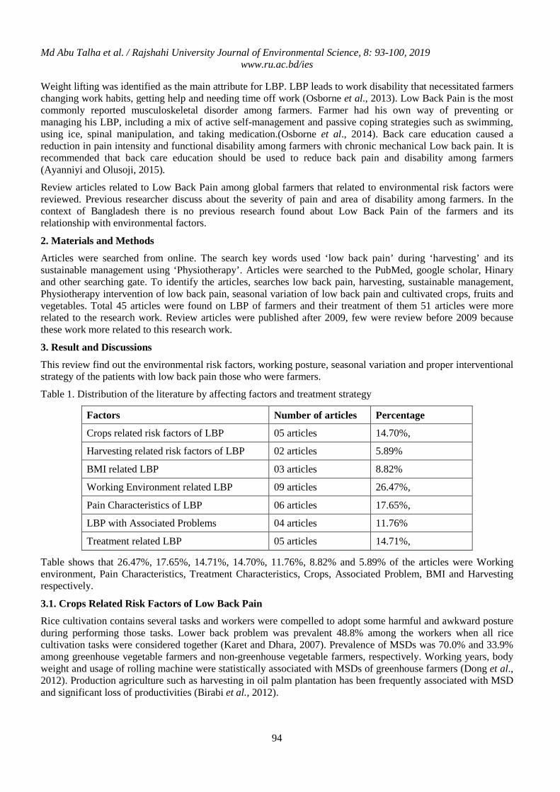
Md Abu Talha et al. / Rajshahi University Journal of Environmental Science, 8: 93-100, 2019 www.ru.ac.bd/ies
94
Weight lifting was identified as the main attribute for LBP. LBP leads to work disability that necessitated farmers changing work habits, getting help and needing time off work (Osborne et al., 2013). Low Back Pain is the most commonly reported musculoskeletal disorder among farmers. Farmer had his own way of preventing or managing his LBP, including a mix of active self-management and passive coping strategies such as swimming, using ice, spinal manipulation, and taking medication.(Osborne et al., 2014). Back care education caused a reduction in pain intensity and functional disability among farmers with chronic mechanical Low back pain. It is recommended that back care education should be used to reduce back pain and disability among farmers (Ayanniyi and Olusoji, 2015).
Review articles related to Low Back Pain among global farmers that related to environmental risk factors were reviewed. Previous researcher discuss about the severity of pain and area of disability among farmers. In the context of Bangladesh there is no previous research found about Low Back Pain of the farmers and its relationship with environmental factors.
2. Materials and Methods
Articles were searched from online. The search key words used ‘low back pain’ during ‘harvesting’ and its sustainable management using ‘Physiotherapy’. Articles were searched to the PubMed, google scholar, Hinary and other searching gate. To identify the articles, searches low back pain, harvesting, sustainable management, Physiotherapy intervention of low back pain, seasonal variation of low back pain and cultivated crops, fruits and vegetables. Total 45 articles were found on LBP of farmers and their treatment of them 51 articles were more related to the research work. Review articles were published after 2009, few were review before 2009 because these work more related to this research work.
3. Result and Discussions
This review find out the environmental risk factors, working posture, seasonal variation and proper interventional strategy of the patients with low back pain those who were farmers.
Table 1. Distribution of the literature by affecting factors and treatment strategy
Factors Number of articles Percentage Crops related risk factors of LBP 05 articles 14.70%, Harvesting related risk factors of LBP 02 articles 5.89% BMI related LBP 03 articles 8.82% Working Environment related LBP 09 articles 26.47%, Pain Characteristics of LBP 06 articles 17.65%, LBP with Associated Problems 04 articles 11.76% Treatment related LBP 05 articles 14.71%,
Table shows that 26.47%, 17.65%, 14.71%, 14.70%, 11.76%, 8.82% and 5.89% of the articles were Working environment, Pain Characteristics, Treatment Characteristics, Crops, Associated Problem, BMI and Harvesting respectively.
3.1. Crops Related Risk Factors of Low Back Pain
Rice cultivation contains several tasks and workers were compelled to adopt some harmful and awkward posture during performing those tasks. Lower back problem was prevalent 48.8% among the workers when all rice cultivation tasks were considered together (Karet and Dhara, 2007). Prevalence of MSDs was 70.0% and 33.9% among greenhouse vegetable farmers and non-greenhouse vegetable farmers, respectively. Working years, body weight and usage of rolling machine were statistically associated with MSDs of greenhouse farmers (Dong et al., 2012). Production agriculture such as harvesting in oil palm plantation has been frequently associated with MSD and significant loss of productivities (Birabi et al., 2012).
Md Abu Talha et al. / Rajshahi University Journal of Environmental Science, 8: 93-100, 2019 www.ru.ac.bd/ies
95
Rice farmers often have poor sustained postures during a rice planting process and start their farming at an early age. However, individual associated factors of Clinical lumbar instability were known and have rarely been diagnosed in low back pain (Puntumetakul et al., 2015). Low back pain is common among rubber farmers, postural factors were identified as being associated with the high prevalence of LBP (Udom et al., 2016).
3.2. Harvesting Related Risk Factors
Back pain is the most prevalent occupational health problem experienced by much of the world's workforce. However, agricultural work-related back pains occurring among US farmers and it was 26.2%. These findings were significant positive associations between depression, farming activities, and back pain (Xiang et al., 1999).The prevalence of Clinical lumbar instability in Thai rice farmers was 13% their mean age were 44±10 years. Number of years of farming experience was found to be significantly correlated with the prevalence of Clinical lumbar instability (Puntumetakul et al., 2015).
3.3. Body Mass Index Related Low Back Pain
Low back pain was more prevalent in who had farming for a long duration. Severe LBP was significantly linked with age group, low BMI and those above average height was 1.60 m (Birabi et al., 2012). Low back pain is one of the most prevalent musculoskeletal disorders in the general population, especially among manual laborers BMI, exposure to pesticides, and tapping below knee level were statistically associated (Udom, 2016).
3.4. Working Environment Related Low Back Pain
Farmers showed higher prevalence changes for intervertebral disc disorders than other occupational workers (Cha et al., 2009). The frequency of back pain is related with whole body vibration, as well as with prolonged sitting position, wrong body posture and physical work load. The repeated or constant exposure to mechanical shocks may increase the risk of low back pain (Solecki, 2011).
Back pain was 66.0% and it was dependent work quantity and quality the associations between potential risk factors of farming pattern (Wang et al., 2012). Most common musculoskeletal disorders affecting the farmers of Kanpur-Rural, lower back pain were 60%, knee pain were 39%, shoulder pain 22%, neck pain 10%. Poor postures and lack of ergonomic awareness in the farmer was affected (Gupta and Tarique, 2013).There is a high prevalence of LBP among the respondents was 74.4%. Low back pain was described as moderate in 53.4%. Prolonged bending 51.3% was the most related risk factor. A considerable proportion was 65.9% of the respondents were unable to continue some of the previously enjoyed activities. Males had significantly higher prevalence, recurrence and duration of LBP than the females (Tella et al., 2016). Clinical lumbar instability is one of the subgroups of chronic non-specific low back pain. Thai rice farmers often have poor sustained postures during a rice planting process and start their farming at an early age (Puntumetakul et al., 2014).
Prevalence of low back pain was 83.1%. Farmers with high stress levels were more likely to have low back pain and it was associated with the weekly work duration and stress (Keawduangdee et al., 2015). The lower back was 57.7%, followed by shoulders was 44.0%, and neck was 39.6%. MSD prevalence was significantly related to time spent performing biomechanically demanding tasks such as heavy lifting and working with arms overhead (McMillan et al., 2015). Work-related exposures and inflammatory responses might be involved and identify plasma proteins that differentiated farmers with MSD of these protein biomarkers might eventually be used to identify and prevent work-related MSD (Ghafouri et al., 2016). Occupational determinants of health such as vibration, heavy lifting, and awkward postures are important in the development and progression of low back disorders (Trask et al., 2016).
3.5. Pain Characteristics of Low Back Pain
The most commonly experienced MSDs were back pain 37% and neck/shoulder pain 25%. Other MSDs experienced in the previous year included knee pain 9%, hand, wrist and elbow pain 9%, ankle/foot pain 9% and hip pain 8%. Back pain was more prevalent in full time farmer, while prevalence of hip pain was greater in farmers who were older, full time, farming for longer and working for longer hours (Osborn et al., 2010). Prevalence rates of LBP were 77%, 56% and 49%, respectively. No relationship between age and LBP was found. Ninety-five percent of LBP were chronic, experiencing pain longer than 12 weeks with a mean duration was 5.6 years (Taechasubamorn et al., 2011). Prevalence of MSD among farmers was 90.6% while 1-year MSD
Md Abu Talha et al. / Rajshahi University Journal of Environmental Science, 8: 93-100, 2019 www.ru.ac.bd/ies
96
prevalence was 76.9%. LBP prevalence was 75% while 1-year LBP prevalence was 47.8%. The next most common regional MSDs reported range from 10.4-41% to 3.6-71.4% (Osborne et al., 2012).
Farmers experience musculoskeletal symptoms such as pain and disability at a higher rate than other professions. Musculoskeletal symptom prevalence varied by age and joint, with the lowest prevalence of 28% for the elbow and the highest prevalence of over 73% for the lower back (Tonelli et al., 2015). Chronic low back pain prevalence was 8·4%. Increasing age, rearing two or more species of livestock, exposure to tasks that require heavy physical exertion, working in awkward postures, green tobacco sickness, pesticide poisoning, and minor psychiatric disorders were associated with CLBP (Meucci et al., 2015). The prevalence of low back pain was found to be 42%. The majority of women were 60.9% with low back pain experienced moderate disability (Ahdhi et al., 2016).
3.6. Low Back Pain with Associated Problems
The frequency of low back was 63.8%, leg/foot was 43.3%, shoulder was 42.9%, wrist/hand/finger was 26.6%, arm/elbow was 25.3%, and neck was 21.8%. Low back pain was more frequent in those with over 30 years of farming experience (Min et al., 2016). Musculoskeletal pain in multiple areas was 91.3%, and low back pain was 63.8% was the most frequent site of pain. 53% of participants had worked in farming for more than 30 years, and workers involved in dry-field farming comprised the largest subgroup was 41.5% (Jo et al., 2016).
Hormones play an important role in the etiology and pathophysiology of a variety of musculoskeletal degenerative diseases and it accelerated disc degeneration due to relative estrogen deficiency (Wang et al., 2016). Chronic low back pain is a common orthopedic condition that co-exists with depression. The prevalence of depression in patients with CLBP was observed to be 39.5% which is comparable to the reports of previous studies in the developed countries (Namgawa et al., 2016).
3.7. Treatment Related Low Back Pain
Prevention might be more beneficial in the management of LBP. With respect to prevention, the knowledge of risk factors is essential. Exposures involving spinal mechanical load reducing is frequently discussed as a potential benefit for LBP (Bakker et al., 2009). The socio-demographic differences between farmers and non farmers with chronic back disorders may impact the design of effective interventions and have implications for health services planning and health care delivery (Saskatchewan and Josh, 2010). Compared to general exercise, core stability exercise is more effective in decreasing pain and may improve physical function in patients with chronic back pain. There was no significant long-term differences in pain severity were observed between patients who engaged in core stability exercise versus those who engaged in general exercise (Wang et al., 2012). The application of an instruction protocol Intervention for low back pain was effective in improving patient knowledge and practice, with associated amelioration of the severity of pain and disability among them (Taha et al., 2015). Low back pain was found to be a cause of work absenteeism of working population. Fifty percent of the respondents suffered from low back pain. Back care education can be provided to the farmers (Kamruzzaman, 2016).
3.8. Bangladesh Perspectives
Bangladesh is a lower-middle income, most densely populated countries in the world and continues to face numerous political, economic, social and environmental challenges, including political instability, poverty and overpopulation. Food security is also constrained by low level of productivity, profitability, and high yield gap; relatively slow rate of take up of new technologies; inadequate level of private sector interest and investments in agricultural value chain; fluctuations in agricultural production; and limited resources for building resilience to climate change. They suffered different types of disorders including back pain, neck pain, knee pain, wrist and elbow pain due to their working posture, intensive farming and heavy weight lifting and carrying and exposed to different types of health risk type of farming activity. In Bangladesh there is no previous research finding about this risk factors of musculoskeletal disorders of the farmers of rural community.
Md Abu Talha et al. / Rajshahi University Journal of Environmental Science, 8: 93-100, 2019 www.ru.ac.bd/ies
97
4. Conclusion
This review found that working environment, crops pattern, seasonal variation, working hours, working duration, bending posture were the risk factors of Low Back Pain among farmers. Several Physiotherapy intervention strategies were the sustainable management of these issues.
References
Ahdhi GS, Subramanian R, Saya GK and Yamuna TV. 2016. Prevalence of low back pain and its relation to quality of life and disability among women in rural area of Puducherry, India. Indian J. Pain, 30:111-115.
Akinbo TBA, Asafa SRA, Gbiri SA and Ademola C. 2013. Prevalence and impacts of low back pain among peasant farmers in south-west Nigeria. International Journal of Occupational Medicine and Environmental Health, 26(4):621-627.
Ayanniyi O and Olusoji GI. 2015. Back care education on peasant farmers suffering from chronic mechanical low back pain. J. ExpIntegr Med, 5(4): 215-221.
Bakker EW, Verhagen AP, van Trijffel E, Lucas C and Koes BW. 2009. Spinal mechanical load as a risk factor for low back pain: a systematic review of prospective cohort studies. Spine, 34(8):281-93
Birabi BN, Dienye PO and Ndukwu GU. 2012. Prevalence of low back pain among peasant farmers in a rural community in South South Nigeria. Rural and Remote Health, 12:1920.
Cha ES, Kong KA, MoonEK and Lee WJ. 2009. Prevalence and changes in chronic diseases among South Korean farmers: 1998 to 2005. BMC Public Health, 9:268
Dong HY, Li HJ and Yu SF. 2012. Analyzing the factors of influencing the musculoskeletal disorders of greenhouse vegetable farmers. Chinese Journal of Industrial Hygiene and Occupational Diseases, 30(3):198-200.
Ghafouri B, Carlsson A, Holmberg S, Thelin A and Tagesson C. 2016. Biomarkers of systemic inflammation in farmers with musculoskeletal disorders; a plasma proteomic study. BMC Musculoskelet Disorder, 17:206.
Gupta G and Tarique. 2013. Prevalence of Musculoskeletal Disorders in Farmers of Kanpur-Rural, India. J Community Med Health Educ., 3:249.
Holmberg S, Thelin A, Stiernstrom E and Svardsudd K. 2003. The impact of physical work exposure on musculoskeletal symptoms among farmers and rural non-farmers. Ann Agric Environ Med., 10 (2):179-184.
Holmberg S, Thelin A, Stiernström EL and Svärdsudd K. 2004. Psychosocial factors and low back pain, consultations, and sick leave among farmers and rural referents: a population-based study. J Occup Environ Med., 46(9): 993-998.
Holmberg S, Thelin A, Stiernström EL and Svärdsudd K. 2005. Low back pain comorbidity among male farmers and rural referents: a population-based study. Ann Agric Environ Med., 12(2):261-268.
Jo H, Baek S, Park HW, Lee SA, Moon J, Yang JE, Kim KS, Kim JY and Kang EK. 2016. Farmers' Cohort for Agricultural Work-Related Musculoskeletal Disorders (FARM) Study: Study Design, Methods, and Baseline Characteristics of Enrolled Subjects. J Epidemiol., 26(1):50-56.
Kamruzzaman M. 2016. Prevalence of Low Back Pain among Farmers. EC Orthopaedics, 2(6): 218-221.
Kar SK and Dhara PC. 2007. An evaluation of musculoskeletal disorder and socioeconomic status of farmers in West Bangal, India. Nepal Medical College Journal, 9(4): 245-249.
Keawduangdee P, Puntumetakul R, Swangnetr M, Laohasiriwong W, Settheetham D, Yamauchi J and Boucaut R. 2015. Prevalence of low back pain and associated factors among farmers during the rice transplanting process. J PhysTher Sci., 27(7):2239-45.
Md Abu Talha et al. / Rajshahi University Journal of Environmental Science, 8: 93-100, 2019 www.ru.ac.bd/ies
98
McMillan M, Trask C, Dosman J, Hagel L and Pickett W. 2015. Saskatchewan Farm Injury Cohort Study Team. Prevalence of Musculoskeletal Disorders Among Saskatchewan Farmers. J Agromedicine, 20(3):292-301.
Meucci RD, Fassa AG, Faria NM and Fiori NS. 2015. Chronic low back pain among tobacco farmers in southern Brazil. Int J Occup Environ Health, 21(1):66-73.
Min D, Baek S, Park HW, Lee SA, Moon J, Yang JE, Kim KS, Kim JY and Kang EK. 2016. Prevalence and Characteristics of Musculoskeletal Pain in Korean Farmers. Ann Rehabil Med., 40(1):1-13.
Murtezani A, Hundozi H, Orovcanec N, Berisha M and Meka V. 2010. Low back pain predict sickness absence among power plant workers. Indian J Occup Environ Med., 14:49-53.
Namgwa KJ, Terkura A, William Y, Daniel MD and Cornilius EI. 2016. Depression in patients with chronic low back pain: A hospital-based study. Niger J Surg Res., 17:1-4.
Ogunbode AM, Adebusoye LA and Alonge TO. 2013. Prevalence of low back pain and associated risk factors amongst adult patients presenting to a Nigerian family practice clinic, a hospital-based study. Afr J Prm Health Care Fam Med., 5(1):441-448.
Osborne A, Blake C, Fullen BM, Meredith D, Phelan J, McNamara J and Cunningham C. 2012. Prevalence of musculoskeletal disorders among farmers: A systematic review. Am J Ind Med., 55(2):143-158.
Osborne A, Blake C, McNamara J, Meredith D, Phelan J and Cunningham C. 2010. Musculoskeletal disorders among Irish farmers. Occupational Medicine Advance Access published, 15(9):1-6.
Osborne A, Blake C, Meredith D, McNamara J, Phelan J and Cunningham C. 2014. The Lived Experience of Low Back Pain among Irish Farmers: Case Studies. Journal of Agromedicine, 19(2):181-190.
Osborne A, Finnegan G, Blake C, Meredith D, McNamara J, Phelan J and Cunningham C. 2013. An evaluation of low back pain among farmers in Ireland. Occup Med. (Lond), 63(1):53-59.
Park JS and Oh GJ. 2008. Differences in Farmer's Syndrome between Greenhouse-Melon Farmers and Rice Farmers. J Agric Med Community Health, 33(1):27-36.
Puntumetakul R, Yodchaisarn W, Emasithi A, Keawduangdee P, Chatchawan U and Yamauchi J. 2015. Prevalence and individual risk factors associated with clinical lumbar instability in rice farmers with low back pain. Patient Preference and Adherence, 9:1-7.
Puntumetakul R, Yodchaisarn W, Emasithi A, Keawduangdee P, Chatchawan U and Yamauchi J. 2014. Prevalence and individual risk factors associated with clinical lumbar instability in rice farmers with low back pain. Patient Preference and Adherence, 9:1-7.
Rosecrance J, Rodgers G and Merlino L. 2006. Low back pain and musculoskeletal symptoms among Kansas farmers. Am J Ind Med., 49(7):547-556.
Saskatchewan and Lawson J. 2014. A Profile of Farmers and Other Employed Canadians with Chronic Back Pain: A Population-Based Analysis of the 2009-2010 Canadian Community Health Surveys. The Journal of Rural Health, 30(3):300-31.
Solecki L. 2011. Low back pain among farmers exposed to whole body vibration: a literature review. Med Pr., 62(2):187-202.
Taechasubamorn P, Nopkesorn T and Pannarunothai S. 2011. Prevalence of Low Back Pain among Rice Farmers in a Rural Community in Thailand. Med Assoc Thai, 94(5):616-622.
Taha NM, Mohamed NA and El-Aziz NAA. 2015. Nursing intervention protocol for adult patients experiencing chronic low back pain. Cent. EJN, 6(4):343-351.
Tamrin SBM, Yik WM, Yusoff ISM and Mor I. 2014. The Prevalence of Musculoskeletal Disorder and Association with Productivity Loss: A Preliminary Study among Labour Intensive Manual Harvesting Activities in Oil Palm Plantation Yee Guan NG. Industrial Health, 52:78-85.
Md Abu Talha et al. / Rajshahi University Journal of Environmental Science, 8: 93-100, 2019 www.ru.ac.bd/ies
99
Tella BA, Akinbo SRA and Asafa SA. 2016. Prevalence and impacts of low back pain among peasant farmers in South-West Nigeria. Afr. J. Biomed Res., 19(5):109-115.
Tonelli S, Culp K and Donham KJ. 2015. Prevalence of Musculoskeletal Symptoms and Predictors of Seeking Healthcare among Iowa Farmers. J. Agric. Saf. Health, 21(4):229-39.
Trask C, Bath B, Johnson PW, Teschke K. 2016. Risk Factors for Low Back Disorders in Saskatchewan Farmers: Field-based Exposure Assessment to Build a Foundation for Epidemiological Studies. JMIR Res Protoc, 5(2), doi: 10.2196/resprot. 5573.
Udom C, Janwantanakul P and Kanlayanaphotporn R. 2016. The Prevalence of Low Back Pain and its Associated Factors in Thai Rubber Farmers. J Occup Health, 58(6):534-542.
Wang LX, Stallones L, Wheeler L, Zhao KK, Smith W and Xiang GA. 2012. Back Pain among Farmers in a Northern Area of China. Spine, 37(6):508-514.
Wang X-Q, Zheng J-J, Yu Z-W, Bi X, Lou S-J and Liu J. 2012. A Meta-Analysis of Core Stability Exercise versus General Exercise for Chronic Low Back Pain. PLoS ONE, 7(12).
Wang Y-X, Wang J and Kaplar Z. 2016. Increased low back pain prevalence in females than in males after menopause age: evidences based on synthetic literature review. Quant Imaging Med. Surg, 6(2):199-206.
Wiley-Liss. 2006. Low back pain and musculoskeletal symptoms among Kansas farmers. American journal of Industrial Medicine, 49(7):547-556.
Xiang H, Stallones L and Keefe TJ. 1999. Back pain and agricultural work among farmers: An analysis of the Colorado Farm Family Health and Hazard Surveillance Survey. Am J Ind Med., 35(3):310-316.
Yonelia, A.L and Kurniawidjaja, M. 2013. Risk Management of Occupational Health and Safety in Rice Farmers in Ngrendeng, East Java in 2012. International Journal on Advanced Science, Engineering and Information Technology, 3(1):28-32.

Md Abu Talha et al. / Rajshahi University Journal of Environmental Science, 8: 93-100, 2019 www.ru.ac.bd/ies
100
Md. Ruhul Amin et al. / Rajshahi University Journal of Environmental Science, 8: 101-110, 2019 www.ru.ac.bd/ies
Effect of Weather Conditions on Stroke: A Review
Md. Ruhul Amin1∗, Md. Redwanur Rahman1, Md. Moniruzzaman Sarker2, Md. Nurul Islam3
and Tanvir Haider4
1* Institute of Environmental Science, University of Rajshahi, Bangladesh
2 Department of Zoology, University of Rajshahi, Bangladesh
3 Department of Medicine, Rajshahi Medical College and Hospital, Bangladesh 4 National Institute of Neurosciences and Hospital, Dhaka, Bangladesh
Abstract
Stroke is a focal episode of neurological deficit and brain tissue damage, either infraction or hemorrhage which persists for more than 24 hours and resultant weaknesses the half of the body. The objectives of the study to review the weather condition related to risk factors of stroke. This reviewed mainly focuses on weather conditions-related articles, which are mainly related to stroke. A literatures search of online database has been performed from July 2019 and the study found the association among risk factors related variables and stroke and its remedies. Reviewed articles show that 41.8, 21.8, 12.7, 9,1, 9.1, and 5.5% had a temperature, atmospheric pressure, humidity, snowfall and rainfall, seasonal variation, and air pollution-related respectively. It was found from the review that low temperature, low atmospheric pressure, and less humidity were responsible for intracerebral hemorrhage contrast to the ischemic stroke it may have occurred at high temperature, high atmospheric pressure, and more humid conditions. However, the mean lowest temperatures of stroke occurrence had 1.33°C, and the mean highest temperature of stroke occurrence had 14.50°C and a range between -20°C and 30°C.
Keywords: Stroke; Weather Conditions; Seasonal Variation.
1. Introduction
Health is an important issue and needs special attention to their medical checkup but in our country, there are no formal health checkup facilities for this risk factor did not find out and non-communicable diseases suddenly attack human health, stroke is one of them. Stroke is a focal episode of neurological deficit and damage of brain tissue, either due to infarction or hemorrhage which persists more than 24 hours. Ischemic, hemorrhagic, and transient ischemic attacks were common types (Hauser, 2010). History of hypertension, diabetes mellitus, central obesity, psychosocial stress, and smoking were the risk factors of ischemic stroke, whereas alcohol intake was the risk factor for haemorrhagic stroke (Donnel et al., 2010). External stimuli, such as temperature, atmospheric pressure, and humidity were responsible for stroke (Cao et al., 2016). High annual rainfall, average temperature, cold days may affect the risk of stroke (Matsumoto et al., 2010). Higher body temperature resulting in excess fluid loss causes hemoconcentration, which increased the incidence of ischemic stroke (Kvistood et al., 2012). The high and low temperature was directly influenced by the risk of stroke (Chen et al., 2013). Maximum temperature and atmospheric pressure combined with a significant predictor of stroke. Daily fluctuations in atmospheric pressure also had significant effects on stroke incidence (Nocera et al., 2014). Hurricanes or tropical storms increased the risk of ischemic stroke but daily lowest and highest air pressure and temperature fall in both ischemic and subarachnoid hemorrhages (Tarnoki et al., 2017). Stroke is the leading cause of death and disability in Bangladesh. Rehabilitation services have few yet integrated into the Bangladesh health system. Only a few government and non-governmental organizations provide rehabilitation for stroke patients (Mamin et al., 2017).
Stroke causes impairments, long-term disability resulting from lead to persistent difficulties with walking. After a stroke, secondary complications may arise such as joints contracture and deformity, heart disease, bedsore, urinary tract infection, respiratory infection were more common (Eng and Tang, 2007). Stroke is one of the top 5 leading causes of death and one of the top 10 causes of hospitalization in Malaysia with the greatest burden of disease based on disability (Loo and Gan, 2012). In the Philippines, the prevalence ranged from 1·9 to 6·59%, and the government should emphasize primary and secondary prevention strategies (Loo and Gan, 2013). In India, China, Philippines, Thailand, Sri Lanka, Iran, Pakistan, Nepal, there has been a rapid increase in stroke
∗ Corresponding author’s e-mail: [email protected]
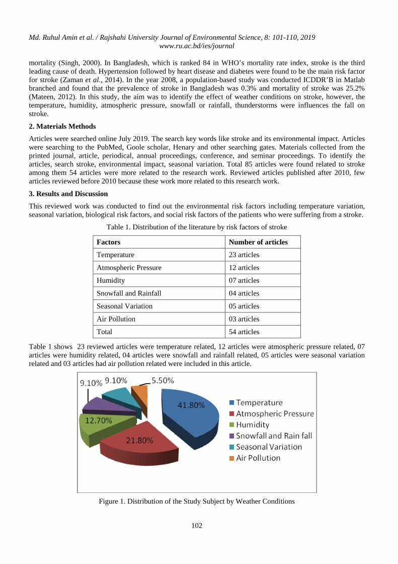
Md. Ruhul Amin et al. / Rajshahi University Journal of Environmental Science, 8: 101-110, 2019 www.ru.ac.bd/ies/journal
102
mortality (Singh, 2000). In Bangladesh, which is ranked 84 in WHO’s mortality rate index, stroke is the third leading cause of death. Hypertension followed by heart disease and diabetes were found to be the main risk factor for stroke (Zaman et al., 2014). In the year 2008, a population-based study was conducted ICDDR’B in Matlab branched and found that the prevalence of stroke in Bangladesh was 0.3% and mortality of stroke was 25.2% (Mateen, 2012). In this study, the aim was to identify the effect of weather conditions on stroke, however, the temperature, humidity, atmospheric pressure, snowfall or rainfall, thunderstorms were influences the fall on stroke.
2. Materials Methods
Articles were searched online July 2019. The search key words like stroke and its environmental impact. Articles were searching to the PubMed, Goole scholar, Henary and other searching gates. Materials collected from the printed journal, article, periodical, annual proceedings, conference, and seminar proceedings. To identify the articles, search stroke, environmental impact, seasonal variation. Total 85 articles were found related to stroke among them 54 articles were more related to the research work. Reviewed articles published after 2010, few articles reviewed before 2010 because these work more related to this research work.
3. Results and Discussion
This reviewed work was conducted to find out the environmental risk factors including temperature variation, seasonal variation, biological risk factors, and social risk factors of the patients who were suffering from a stroke.
Table 1. Distribution of the literature by risk factors of stroke
Factors Number of articles Temperature 23 articles Atmospheric Pressure 12 articles Humidity 07 articles Snowfall and Rainfall 04 articles Seasonal Variation 05 articles Air Pollution 03 articles Total 54 articles
Table 1 shows 23 reviewed articles were temperature related, 12 articles were atmospheric pressure related, 07 articles were humidity related, 04 articles were snowfall and rainfall related, 05 articles were seasonal variation related and 03 articles had air pollution related were included in this article.
Figure 1. Distribution of the Study Subject by Weather Conditions
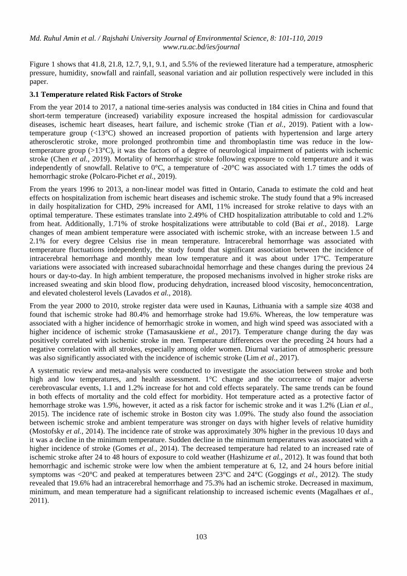
Md. Ruhul Amin et al. / Rajshahi University Journal of Environmental Science, 8: 101-110, 2019 www.ru.ac.bd/ies/journal
103
Figure 1 shows that 41.8, 21.8, 12.7, 9,1, 9.1, and 5.5% of the reviewed literature had a temperature, atmospheric pressure, humidity, snowfall and rainfall, seasonal variation and air pollution respectively were included in this paper.
3.1 Temperature related Risk Factors of Stroke
From the year 2014 to 2017, a national time-series analysis was conducted in 184 cities in China and found that short-term temperature (increased) variability exposure increased the hospital admission for cardiovascular diseases, ischemic heart diseases, heart failure, and ischemic stroke (Tian et al., 2019). Patient with a low-temperature group (<13°C) showed an increased proportion of patients with hypertension and large artery atherosclerotic stroke, more prolonged prothrombin time and thromboplastin time was reduce in the low-temperature group (>13°C), it was the factors of a degree of neurological impairment of patients with ischemic stroke (Chen et al., 2019). Mortality of hemorrhagic stroke following exposure to cold temperature and it was independently of snowfall. Relative to 0°C, a temperature of -20°C was associated with 1.7 times the odds of hemorrhagic stroke (Polcaro-Pichet et al., 2019).
From the years 1996 to 2013, a non-linear model was fitted in Ontario, Canada to estimate the cold and heat effects on hospitalization from ischemic heart diseases and ischemic stroke. The study found that a 9% increased in daily hospitalization for CHD, 29% increased for AMI, 11% increased for stroke relative to days with an optimal temperature. These estimates translate into 2.49% of CHD hospitalization attributable to cold and 1.2% from heat. Additionally, 1.71% of stroke hospitalizations were attributable to cold (Bai et al., 2018). Large changes of mean ambient temperature were associated with ischemic stroke, with an increase between 1.5 and 2.1% for every degree Celsius rise in mean temperature. Intracerebral hemorrhage was associated with temperature fluctuations independently, the study found that significant association between the incidence of intracerebral hemorrhage and monthly mean low temperature and it was about under 17°C. Temperature variations were associated with increased subarachnoidal hemorrhage and these changes during the previous 24 hours or day-to-day. In high ambient temperature, the proposed mechanisms involved in higher stroke risks are increased sweating and skin blood flow, producing dehydration, increased blood viscosity, hemoconcentration, and elevated cholesterol levels (Lavados et al., 2018).
From the year 2000 to 2010, stroke register data were used in Kaunas, Lithuania with a sample size 4038 and found that ischemic stroke had 80.4% and hemorrhage stroke had 19.6%. Whereas, the low temperature was associated with a higher incidence of hemorrhagic stroke in women, and high wind speed was associated with a higher incidence of ischemic stroke (Tamasauskiene et al., 2017). Temperature change during the day was positively correlated with ischemic stroke in men. Temperature differences over the preceding 24 hours had a negative correlation with all strokes, especially among older women. Diurnal variation of atmospheric pressure was also significantly associated with the incidence of ischemic stroke (Lim et al., 2017).
A systematic review and meta-analysis were conducted to investigate the association between stroke and both high and low temperatures, and health assessment. 1°C change and the occurrence of major adverse cerebrovascular events, 1.1 and 1.2% increase for hot and cold effects separately. The same trends can be found in both effects of mortality and the cold effect for morbidity. Hot temperature acted as a protective factor of hemorrhage stroke was 1.9%, however, it acted as a risk factor for ischemic stroke and it was 1.2% (Lian et al., 2015). The incidence rate of ischemic stroke in Boston city was 1.09%. The study also found the association between ischemic stroke and ambient temperature was stronger on days with higher levels of relative humidity (Mostofsky et al., 2014). The incidence rate of stroke was approximately 30% higher in the previous 10 days and it was a decline in the minimum temperature. Sudden decline in the minimum temperatures was associated with a higher incidence of stroke (Gomes et al., 2014). The decreased temperature had related to an increased rate of ischemic stroke after 24 to 48 hours of exposure to cold weather (Hashizume et al., 2012). It was found that both hemorrhagic and ischemic stroke were low when the ambient temperature at 6, 12, and 24 hours before initial symptoms was <20°C and peaked at temperatures between 23°C and 24°C (Goggings et al., 2012). The study revealed that 19.6% had an intracerebral hemorrhage and 75.3% had an ischemic stroke. Decreased in maximum, minimum, and mean temperature had a significant relationship to increased ischemic events (Magalhaes et al., 2011).
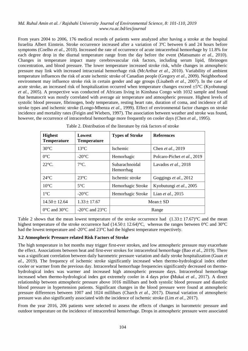
Md. Ruhul Amin et al. / Rajshahi University Journal of Environmental Science, 8: 101-110, 2019 www.ru.ac.bd/ies/journal
104
From years 2004 to 2006, 176 medical records of patients were analyzed after having a stroke at the hospital Israelita Albert Einstein. Stroke occurrence increased after a variation of 3ºC between 6 and 24 hours before symptoms (Coelho et al., 2010). Increased the rate of occurrence of acute intracerebral hemorrhage by 11.8% for each degree drop in the diurnal temperature range from the day before the event (Matsumato et al., 2010). Changes in temperature impact many cerebrovascular risk factors, including serum lipid, fibrinogen concentration, and blood pressure. The lower temperature increased stroke risk, while changes in atmospheric pressure may link with increased intracranial hemorrhage risk (McArthur et al., 2010). Variability of ambient temperature influences the risk of acute ischemic stroke of Canadian people (Gregory et al., 2009). Neighborhood environment may influence stroke risk in certain gender and age groups (Lisabeth et al., 2007). In the case of acute stroke, an increased risk of hospitalization occurred when temperature changes exceed ±5°C (Kyobutungi et al., 2005). A prospective was conducted of Africans living in Kinshasa Congo with 1032 sample and found that hematocrit was mostly correlated with average air temperature and atmospheric pressure. Highest levels of systolic blood pressure, fibrinogen, body temperature, resting heart rate, duration of coma, and incidence of all stroke types and ischemic stroke (Longo-Mbenza et al., 1999). Effect of environmental factor changes on stroke incidence and mortality rates (Feigin and Wiebers, 1997). The association between weather and stroke was found, however, the occurrence of intracerebral hemorrhage more frequently on cooler days (Chen et al., 1995).
Table 2. Distribution of the literature by risk factors of stroke
Highest Temperature
Lowest Temperature
Types of Stroke References
30°C 13°C Ischemic Chen et al., 2019 0°C -20°C Hemorhagic Polcaro-Pichet et al., 2019 22°C. 7°C. Subarachnoidal
Hemorrhag Lavados et al., 2018
24°C 23°C Ischemic stroke Goggings et al., 2012 10°C 5°C Hemorhagic Stroke Kyobutungi et al., 2005 1°C -20°C Hemorhagic Stroke Lian et al., 2015 14.50± 12.64 1.33± 17.67 Mean± SD 0°C and 30°C -20°C and 23°C Range
Table 2 shows that the mean lowest temperature of the stroke occurrence had (1.33± 17.67)°C and the mean highest temperature of the stroke occurrence had (14.50± 12.64)°C, whereas the ranges between 0°C and 30°C had the lowest temperature and -20°C and 23°C had the highest temperature respectively.
3.2 Atmospheric Pressure related Risk Factors of Stroke
The high temperature in hot months may trigger first-ever strokes, and low atmospheric pressure may exacerbate the effect. Associations between heat and first-ever strokes for intracerebral hemorrhage (Bao et al., 2019). There was a significant correlation between daily barometric pressure variation and daily stroke hospitalization (Guan et al., 2019). The frequency of ischemic stroke significantly increased when thermo-hydrological index either cooler or warmer from the previous day. Intracerebral hemorrhage frequencies significantly decreased on thermo-hydrological index was warmer and increased high atmospheric pressure days. Intracerebral hemorrhage increased when thermo-hydrological index got extremely cooler in 4 days prior (Mukai et al., 2017). A direct relationship between atmospheric pressure above 1016 millibars and both systolic blood pressure and diastolic blood pressure in hypertension patients. Significant changes in the blood pressure were found at atmospheric pressure differences between 1007 and 1024 millibars (Charch et al., 2017). Diurnal variation of atmospheric pressure was also significantly associated with the incidence of ischemic stroke (Lim et al., 2017).
From the year 2016, 206 patients were selected to assess the effects of changes in barometric pressure and outdoor temperature on the incidence of intracerebral hemorrhage. Drops in atmospheric pressure were associated
Md. Ruhul Amin et al. / Rajshahi University Journal of Environmental Science, 8: 101-110, 2019 www.ru.ac.bd/ies/journal
105
with different types of intracerebral hemorrhage (Honig et al., 2016). Increased 1hPa in atmospheric pressure for the risk of ischemic stroke, intracerebral hemorrhage, and subarachnoid hemorrhage. It was also revealed that 1 percent increased humidity for risk of ischemic stroke and intracerebral hemorrhage (Cao et al., 2016). It was observed that a significant difference in blood pressure was recorded during the lower and higher range of atmospheric pressure. A significant inverse relationship between atmospheric pressure and blood pressure was identified (Kaminski et al., 2016).
Non-lacunar stroke was related to a fall in atmospheric pressure, while intracerebral hemorrhage was associated with rising atmospheric pressure. However non-lacunar stroke was related to rising in temperature and intracerebral hemorrhage was associated with a fall in temperature (Jimenez-Conde et al., 2008). It was revealed that 90% of the patients suffered from ischemic stroke, 34% were lacunar, 10% had a hemorrhagic stroke. Increased temperature in the risk of ischemic stroke and decreased atmospheric pressure increased the rate of hemorrhagic stroke (Dawson et al., 2007). There was a significant correlation between decreased atmospheric pressure and AMI and no correlation between decreased atmospheric pressure and stroke (Houck et al., 2005). There was a relationship between high atmospheric pressure and increased incidence of subarachnoid hemorrhage (Buxton et al., 2001).
3.3 Humidity related Risk Factors of Stroke
In the year 2004 to 2006, a retrospective study was conducted with a sample size 11930 and found that rapid increases or rapidly decreased in humidity increased the incidence of stroke. Extremely low and high humidity influences the increased number of strokes (Slatina et al., 2013). Decreases in temperature and humidity on the day of or day before stroke have been significantly linked to ischemic stroke and transient ischemic attack (Petrov et al., 2011). Cerebral infraction correlated with more humidity factors, fewer sunshine hours, fewer solar radiation factors, and greater amount of precipitation (Ebi et al., 2004).
3.4 Snowfall and Rainfall related Risk Factors of Stroke
Lower temperature and radical humidity change were identified as risk factors for stroke and a decreasing temperature was also associated (Matsumaru et al., 2020). Sudden cold water exposure increases sympathetic tone, which is mediated by thermo-receptors, activated by the rapid fall in skin temperature, it induced an increase in blood pressure and this cause fall in stroke in high-risk individuals (Benedict and Pandian, 2014). The mortality increased on days of extreme cold conditions. Snowfall was greater than 3cm and when the temperature below -7°C and mortality due to ischemic heart diseases and cerebrovascular cause (Gorjanc et al., 1999). There was a statistically significant negative correlation between mean temperature with admission for cerebrovascular diseases, intracerebral hemorrhage, ischemic stroke, and transient ischemic attack, these correlations were independent of any seasonal variation (Azevedo et al., 1995).
3.5 Seasonal Variation related Risk Factors of Stroke
From the year 2006 to 2007, a survey was conducted among 2319 stroke patients in Wujin, a city, southeast China to evaluate seasonal variations in stroke incidence. Stroke incidence was highest in September and lowest in January, however, autumn had the highest incidence of both ischemic and cerebral hemorrhage (Jin et al., 2018). Cardioembolic stroke was more common in winter. Ischemic stroke patients had more moderate to severe initial neurological deficits in winter and spring and ischemic stroke was not winter dominant disease (Toyoda et al., 2018). There was a higher frequency of stroke in the United State in winter and it was 116862 in winter, 113689 in spring, 113569 in summer, and 113518 in the fall season. Wormer and wetter weather conditions were independently associated with better outcomes (Chu et al., 2018). There were more strokes in winter (December-March) than summer (June-September) (Mateen, 2012). There was no association between weather changes and stroke occurrence (Field and Hill, 2002).
3.6 Air Pollution related Factors of Stroke
Air pollution (sulfur dioxide, nitrogen dioxide, and carbon monoxide) was positively associated with ischemic stroke, whereas only a significant association with nitrogen dioxide and hemorrhagic stroke (Liu et al., 2017). There was a negative correlation between average temperature and intracerebral hemorrhage whole only ozone was independently associated with subarachnoidal hemorrhage (Han et al., 2016). The study showed that
Md. Ruhul Amin et al. / Rajshahi University Journal of Environmental Science, 8: 101-110, 2019 www.ru.ac.bd/ies/journal
106
exposure of particulate mattress 12 to 14 hours greater risk of ischemic stroke and it was PM 2.5 (Wellenius et al., 2012).
3.7 Research Gap
In a nutshell, it was found some gaps while critically reviewing evidence-based paper. Authors of reviewed articles from different countries emphasize on risk factors of stroke and climatic variables of South Asian countries, African countries, the United Kingdom, and the United State of America. In the context of Bangladesh, there was no previous study found regarding the effect of weather conditions on stroke.
3.8 Conclusion
The study concludes that atmospheric pressure, humidity, snowfall, or rainfall, temperature including heat and cold exposure also seasonal variations were the risk factors of stroke.
3.9 Recommendations
Based on the review findings, the following recommendations made to prevent and reduce the risk of stroke.
1. Raising awareness among the population about the risk factors of stroke and its severity
2. A continuous health education program by using print media and electronic media
3. Further study is needed to assess climatic and geographical risk factors of stroke patients in Bangladesh.
References
Azevedo E, Ribeiro JA, Lopes F, Martin R and Barros H. 1995. Cold: arisk factors for stroke? Journal of Neurology, 242: 217-221.
Bai L, Li Q, Wang J, Lavigne E, Gasparrini A and Copes R. 2018. Increased coronary heart diseases and stroke hospitalizations from ambient temperature in Ontario. Heart, 104(8): 673-679.
Bao J, Guo Y, Wang Q, He Y, Ma R and Hua J. 2019. Effects of heat on first-ever stroke and the effect modification of atmospheric pressure: A time-series study in Shenzhen, China. Science of the Total Environment, 654: 1372-1378.
Benedict PS and Pandian JD. 2014. Stroke after cold bath. CHRISMED. 1(4): 283-285.
Buxton N, Liu C, Dasic D, Moody P and Hope DT. 2001. Relationship of aneurismal subarachnoid hemorrhage to changes in atmospheric pressure: results of a prospective study. Journal of Neurosurgery, 95(3): 567-74.
Cao Y, Wang X, Zheng D, Robinson T, Hong D and Richtering S. 2016. Air pressure, humidity and stroke occurrence: A systematic review and meta-analysis. Int. J. Environ., 13: 675-685.
Charch G, Friedman I, Nochomovich H, Rogowski O, Charch R and Steinvil R. 2017. Whether atmospheric pressure changes predict variations in blood pressure. J Cardiol Curr Res., 9(4): 02-06.
Chen ZY, Chang SF and Su CL. 1995. Weather and stroke in a subtropical area: IIan, Taiwan. Home stroke, 26(4): 569-572.
Chen R, Wang C and Meng X. 2013. Both low and high temperature may increase the risk of stroke mortality. Neurology, 81: 1064-1070.
Chen X, Shang W, Huang X, Shu L, Xiao S, Jiang Q and Hong H. 2019. The effect of winter temperature on patients with ischemic stroke. Med. Sci. Monit., 25: 3839-45.
Chu SY, Cox M, Fonarow GC, Smith EE, Schwamm L and Bhatt DL. 2018. Temperature and precipitation associate with ischemic stroke outcome in the United States. Home Journal of American Heart Association, 7(22): 01-10.
Coelho FMS, Santos BFC, Neto MC, Fernando LL, Cypriano AS and Lopes TO. 2010. Temperature variation in the 24 hours before the initial symptoms of stroke. Arq Neuro- Psiquiatr, 68(2): 242-245.
Md. Ruhul Amin et al. / Rajshahi University Journal of Environmental Science, 8: 101-110, 2019 www.ru.ac.bd/ies/journal
107
Dawson J, Weir C, Wright F, Bryden C, Aslanyan S and Lees K. 2007. Associations between meteorological variables and acute stroke hospital admissions in the west of Scotland. Acta Neurol Scan., 117(2): 85-89.
Donnel MJ, Xavier D, Liu L, Zang H, Chin SL and Melacini PR. 2010. Risk factors for ischaemic and intracerebral haemorrhagic stroke in 22 countries (the inter stroke study): a case-control study. The Lancet., 376(9735): 112-123.
Ebi KL, Exuzides KA, Lau E, Kelsh M and Barnston A. 2004. Weather changes associated with hospitalizations for cardiovascular diseases and stroke in California, 1983-98. International Journal of Biometeorology, 49(1): 48-58.
Eng JJ and Tang PF. 2007. Gait training strategies to optimize walking ability in people with stroke: a synthesis of the evidence. Expert Rev Neurother., 7(10): 1417-1436.
Feigin VL and Wiebers DO. 1997. Environmental factors and stroke: A selective review. J Stroke Cerebrovasc Dis., 6(3):108-113.
Field TS and Hill M. 2002. Weather, Chinook, and stroke occurrence. Stroke, 33(7): 1751-1758.
Goggings WB, Woo J, Ho S, Chan EYY and Chau PH. 2012. Weather, season, and daily stroke admissions in Hong Kong. Internation Journal of Biometeorology, 56(5): 865-872.
Gomes J, Damasceno A, Carrilho C, Labo V, Lopes H and Madede T. 2014. The effect of Seasonal and temperature variation on hospital admission for incident stroke events in Maputo, Mozambique. Journal of Stroke and Cerebrovascular Diseases, 23(2): 271-277.
Gorjanc ML, Flanders WD, Vanderslice J, Hersh J and Malilay J. 1999. Effects of temperature and snowfall on mortality in Pennsylvania. Am. J. Epidemiol., 149(12): 1152-60.
Gregory W, Martin OD, Jiming F, Moira K and Murray M. 2009. Temperature and the risk of acute ischemic stroke: results from the registry of the Canadian stroke network. Epidemiology, 20(6): 64-73.
Guan W, Clay SJ, Sloan GJ and Pretlow LG. 2019. Effects of barometric pressure and temperature on acute ischemic stroke hospitalization in August, GA. Translational Stroke Research, 10: 259-64.
Han MH, Yi HJ, Ko Y, Kim YS and Lee YJ. 2016. Association between hemorrhagic stroke occurrence and meteorological factors and pollutants. BMC Neurology, 16(59): 01-08.
Hashizume AHM, Tusda Y, Tsukahara T, Nomiyama T. 2012. Effect of weather variability and air pollutants on emergency admissions for cardiovascular and cerebrovascular diseases. International Journal of Environmental Health Research, 22(5): 416-33.
Hauser SL. 2010. Harrison’s Neurology in Clinical Medicine. 2nd ed. USA: Mc Graw Hill, 246-47, 275-77.
Honig A, Eliahou R, Pikkel YY and Leker RR. 2016. Drops in barometric pressure are associated with deep intracerebral hemorrhage. Journal of Stroke and Cerebrovascular Diseases, 25(4): 872-76.
Houck P, White S, Lethen J, Riggs MW and Gantt DS. 2005. Relation of atmospheric pressure changes and the occurrences of acute myocardial infraction and stroke. The American Journal of Cardiology, 96(1): 45-51.
Jimenez-Conde J, Ois A, Gomis M, Rodriguez-Campello A, Cuadrado-Godia E, Subirana I and Roquer J. 2008. Weather a trigger of stroke. Daily meteorological factors and incidence of stroke subtypes. Cerebrovasc Dis., 26(4): 348-54.
Jin H, Xu Z, Li Y, Xu J, Shan H, Feng X, Xie Y, Bian K and Qin D. 2018. Seasonal variation of stroke incidence in Wujin, a city in southeast China. Health Sci. Rep., 1(4): 29- 35.
Kaminski M, Cieslik-Guerra UI, Kotas R, Mazur P, Maranda W and Piotrowicz M. 2016. Evaluation of the impact of atmospheric pressure in different seasons on blood pressure in patients with arterial hypertension. Int. J. Occup. Med. Environ. Health, 29(5):783-92.
Md. Ruhul Amin et al. / Rajshahi University Journal of Environmental Science, 8: 101-110, 2019 www.ru.ac.bd/ies/journal
108
Kvistood CE, Thomssen L, Andreassen WU and Naess H. 2012. Vascular health and risk management, Neurology, 10(1): 333-338.
Kyobutungi C, Grau A, Stieglbauer G and Becher H. 2005. Absolute temperature, temperature change and stroke risk: a case-crossover study. European Journal of Epidemiology, 20(8): 693-698.
Lavados PM, Olavarria VV and Hoffmeister L. 2018. Ambient temperature and stroke risk. Stroke, 49(1): 255-261.
Lian H, Ruan Y, Liang R, Liu X and Fan Z. 2015. Short-Term Effect of Ambient Temperature and the Risk of Stroke: A Systematic Review and Meta Analysis. International Journal of Environmental Research and Public Health, 12(8): 9068-9088.
Lim JS, Kwon HM, Kim SE, Lee J, Lee YS, and Yoon BW. 2017. Effects of Temperature and Pressure on Acute Stroke Incidence Assessed Using a Korean Nationwide Insurance Database. Journal of Stroke, 19(3): 295-303.
Lisabeth LD, Roux AVD, Escoba JD, Smith MA and Morgenstern LB. 2007. Neighborhood Environment and Risk of Ischemic Stroke: The Brain Attack Surveillance in Corpus Christi (BASIC) Project. American Journal of Epidemiology, 165(3): 279–287.
Liu H, Tian Y, Xu Y, Huang Z, Huang C, Hu Y and Zhang J. 2017. Association between ambient air pollution and hospitalization for ischemic and hemorrhagic stroke in China. Environmental Pollution, 230: 234-241.
Longo-Mbenza B, Phanzu-Mbete LB, M’Buyambo-Kabangu JR, Tonduangu K, Mvunzu M and Muvova D. 1999. Hematocrit and stroke in black African under tropical climate and meteorological influence. Ann. Med. Intern., 150(93) :171-77.
Loo KW and Gan SH. 2012. Burden of stroke in Malaysia. Int. J. Stroke, 7(2):165-67.
Loo KW and Gan SH. 2013. Burden of stroke in the Philippines. Int. J. Stroke, 8(2):131-4.
Magalhaes R, Silva MC, Correia M and Baily T. 2011. Are stroke occurrence and outcome related to weather parameters? Results from a population-based study in northern Portugal. Cerebrovasc Dis., 32(6):542-51.
Mamin FA, Islam MS, Rumana FS and Faruqui F. 2017. Profile of stroke patients treated at a rehabilitation centre in Bangladesh. BMC Research Notes, 10:520.
Mateen, FJ, Carone, M, Alam, N, Streatfield, PK and Black, RE. 2012. A population-based case-control study of 1250 stroke deaths in rural Bangladesh. Eur. J. Neurol., 19(7): 999-1006.
Matsumaru N, Okada H, Suzuki K, Nachi S, Yoshida T, Tsukamoto K and Oguru S. 2020. Weather Fluctuations may have an impact on stroke occurrence in a society: a population- based cohort study. Cerebrovasc Dis. Extra., 10: 01-10.
Matsumato M, Ishikawa S and Kajii E. 2010. Cumulative effects of weather on stroke incidence: a multi-community cohort study in Japan. Journal of Epidemiology, 20(2) : 136-142.
McArthur K, Dawson J and Walter M. 2010. What is it with the weather and stroke?. Expert Rev. Neurother., 10(2):243-49.
Mostofsky E, Wilker EH, Schwartz J, Zanobetti A, Gold DR, Wellenius GA and Mittleman MA. 2014. Short-term changes in ambient temperature and risk of ischemic stroke. Cerebrovasc Dis. Extra., 4(1): 9-18.
Mukai T, Hosomi N, Tsunematsu M, SuedaY, Shimoe Y and Ohshita T. 2017. Various meteorological conditions exhibit both immediate and delayed influences on the risk of stroke events: the Hews-stroke study. PLoS ONE, 12(6): 01-13.
Nocera R, Petrucelli P, Park J and Stander E. 2014. Meteorological Variables Associated with Stroke. International Scholarly Research Notices, 14(33): 1155-1162.
Md. Ruhul Amin et al. / Rajshahi University Journal of Environmental Science, 8: 101-110, 2019 www.ru.ac.bd/ies/journal
109
Petrov D, Hidalgo A, Gandhi C and Prestigiacomo C. 2011. Decreases in temperature and humidity leading to an increased incidence of ischemic stroke. Journal of Neurointerventional Surgery, 3(1): 01-04.
Polcaro-Pichet S, Tomkosatsky, Potter BJ, Bilodeau-Bertrand M and Auger N. 2019. Effects of cold temperature and snow fall on stroke mortality: A case-crossover analysis. Environment International, 126: 89-95.
Singh RB, Suh IL, Singh VP, Chaithiraphan S, Laothavorn P, Sy RG, Babilonia NA, Rahman AR, Sheikh S, Tomlinson B and Sarraf-Zadigan N. 2000. Hypertension and stroke in Asia: prevalence, control and strategies in developing countries for prevention. J. Hum. Hypertens, 14(10-11): 749-63.
Slatina E, Music M, Babic N, Dervisevic A, Mujaric E and Salibasic M. 2013. Correlation between change in air humidity and the incidence of stroke. Mater Sociomed, 25(4): 242-45.
Tamasauskiene L, Rastenyte D, Radisauskas R, Tamosiunas A, Tamasauskas D and Vaiciulis V. 2017. Relationship of metrological factors and acute stroke events in Kaunas (Lithuania) in 2000-2010. Environ. Sci. Pollut. Res. Int., 24(10): 9286-9293.
Tarnoki AD, Türker A, Tarnoki DL, İyisoy MS, Szilagyi BK, Duong H and Miskolczi L. 2017. Relationship between weather conditions and admissions for ischemic stroke and subarachnoid hemorrhage. Croat. Med. J., 58(1): 56–62.
Tian Y, Liu H, Si Y, Cao Y and Song J. 2019. Association between temperature variability and daily hospital admission for case-specific cardiovascular diseases in urban China: A national time-series study. PLOS Medicine, 16(1): 01-07.
Toyoda K, Koga M, Yamagami H, Yokota C, Sato S and Inoue M. 2018. Seasonal variations in neurological severity and outcomes of Ischemic stroke-5- Years single- center observational study. Circ. J. 1231(10): 01-08.
Wellenius GA, Burger MR, Coull BA, Schwart J, Suh HH and Koutrakis P. 2012. Ambient air pollution and the risk of acute ischemic stroke. Arch. Intern. Med., 172(3): 229-234.
Zaman K, Talukder L, Uddin MN, Ahmed T, Islam A and Asaduzzaman M. 2014 Understanding risk factors for stroke death in Bangladesh, International health research in Matlab.

Md. Ruhul Amin et al. / Rajshahi University Journal of Environmental Science, 8: 101-110, 2019 www.ru.ac.bd/ies/journal
110
Kazi Thahamina Akther et al. / Rajshahi University Journal of Environmental Science, 8: 111-120, 2019 www.ru.ac.bd/ies
Suitability and Economic Profitability of Land Conversion for Mango Orchard in Charghat Upazila, Rajshahi
Kazi Thahamina Akther1, S.M. Shafiuzzaman2∗, Md. Sokman Ali1 and Md. Redwanur Rahman2
1Rawtha College, Charghat, Rajshahi, Bangladesh
2Institute of Environmental Science, University of Rajshahi, Rajshahi, Bangladesh
Abstract Orchard has emerged as an important area for alternative cropping pattern due to higher returns and productivity. This study was conducted to determine the suitability and economic profitability of land conversion to mango orchard in Charghat Upazila, Rajshahi. A total 85 mango orchard growing farmers were randomly selected for the interviewing. About (44%) lands were converted to mango orchard from cereal crops. The land conversion was higher in Byaluxmpur (27%), Nimpara (20%) followed by Charghat (14%) union, respectively. The main reason of this conversion was higher quick profit compared to other crops. About 90% farmers have converted crop land into mango orchard because quick profit and economic profitability. Mango orchard farmer obtained an average yield 103 kg/ha mango in 1st quarter (year 1-3) and then production increased sharply to 21694 kg/ha in 5th quarter (year 13-15). Although inter cropping cultivation becomes popular to many farmers because of additional income. While increasing canopy coverage of mango causes yield loss of both rice and other crops. In 15 years, old mango intercrop yield reduces drastically (90%). More than 92% farmers obtained increased income, whereas 77% achieved better livelihoods due to orchard cultivation. However, there is a possibility to decrease of crop land with crop production which may have adverse impact on food security. Therefore, planned mango orchard cultivation is needed along with food security in Charghat Upazila, Rajshahi.
Keywords: Economic Profitability; Land Conversion; Mango Orchard; Crops
1. Introduction The concept sustainable agriculture or farming involves producing quality products in an environmentally benign, socially acceptable and economically efficient way (Addeo et al., 2001). Farmers’ crop diversification decision is considered as one of the important economic decisions which have strong influence on their welfare in terms of income level and returns (Khandoker et al., 2017).With the growth of a country’s economy, agricultural land is usually transferred to non-agriculture as the demand fornon-farmproducts and services increased (Qusasem, 2011). The sustained economic growth, rising per capita income and growing urbanization have caused a shift in the consumption patterns in favor of high value crops like fruits and vegetables from staple food crops such as rice and wheat (Joshi, 2005). While taking decisions farmers make choices in the context of their production possibility frontier, their expectations of relative prices and their sense of risk from both an agronomic and market perspective for various alternatives. The first decision is about the choice of number of crops. While taking decision on number of crops and level of spread in the cropping pattern, farmers also take another critical decision as to which crops to produce and how much land to be allocated to that crop. Hence, the area substitution for crop decision comes from this concept. In recent decades, Charghat Upazila in Rajshahi, demand for mango orchard has grown much faster than that of food grains. In farm planning, farmer decided what to produce, how to produce, and how much to produce (Van and Keller, 2006). The farmer has to decide between alternative uses of resources at his disposal in order to address these three different but inter-related questions. It was observed that in the study area highly unfavorable for crop cultivation and production but favorable production of orchard like mango. Inadequate irrigation management, hard industry, seasonal casual labour shortage, soil nutrient depletionman power less are adding more pressure of farmer on natural resources for sustainable crop production. On the contrary, mango cultivation high productivity and draw quick profit, low water requirement, favorableagro-ecological condition, ready market and also environment friendly farmer’s perception for suitable orchard cultivation. The total agricultural land in the study area has been decreased gradually. Otherwise, orchardland increasing steadily and its production increase sharply. On the other hand, farmer’s discard crop cultivation for years because of lack of justifiable economic return and profitability. Another aspect is the lack of younger generation
∗ Corresponding author’s e-mail: [email protected]
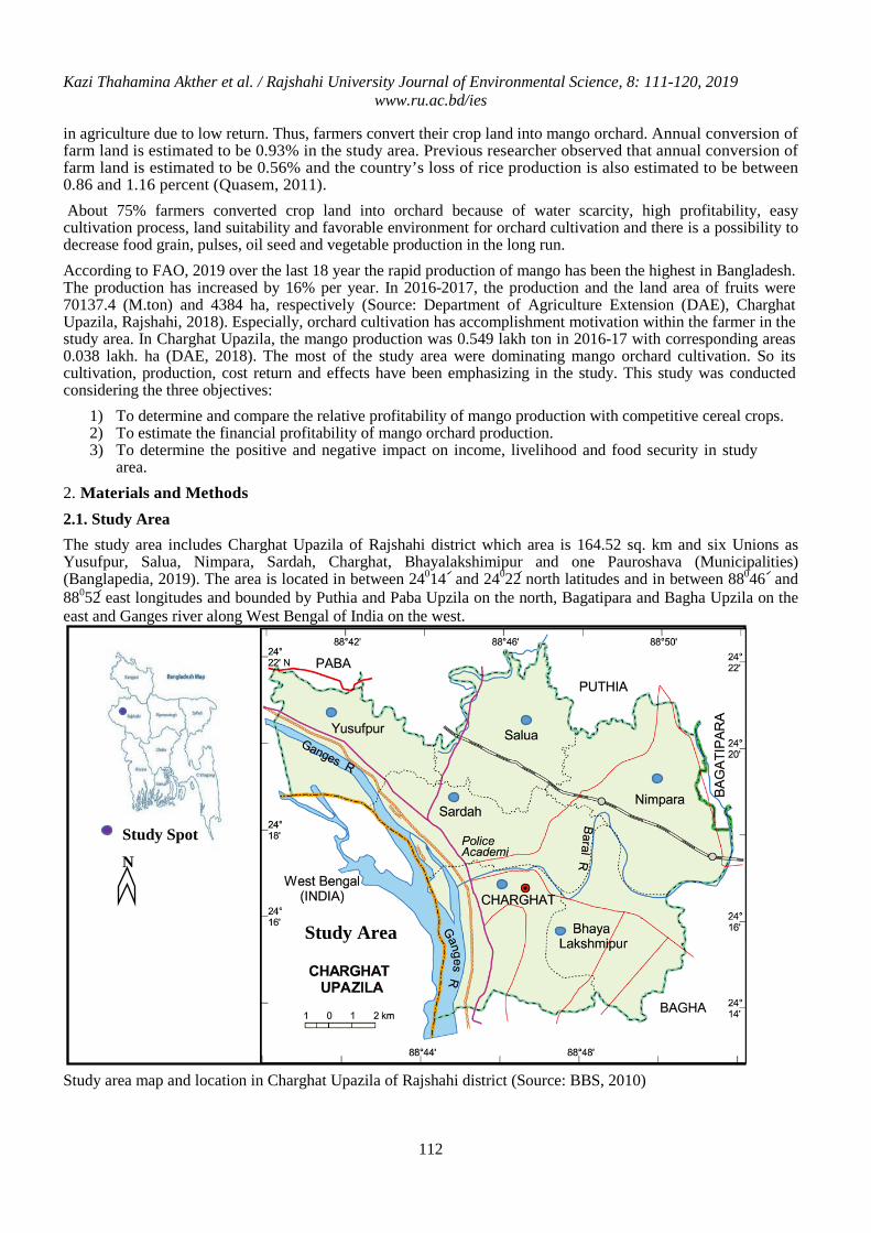
Kazi Thahamina Akther et al. / Rajshahi University Journal of Environmental Science, 8: 111-120, 2019 www.ru.ac.bd/ies
112
in agriculture due to low return. Thus, farmers convert their crop land into mango orchard. Annual conversion of farm land is estimated to be 0.93% in the study area. Previous researcher observed that annual conversion of farm land is estimated to be 0.56% and the country’s loss of rice production is also estimated to be between 0.86 and 1.16 percent (Quasem, 2011). About 75% farmers converted crop land into orchard because of water scarcity, high profitability, easy cultivation process, land suitability and favorable environment for orchard cultivation and there is a possibility to decrease food grain, pulses, oil seed and vegetable production in the long run. According to FAO, 2019 over the last 18 year the rapid production of mango has been the highest in Bangladesh. The production has increased by 16% per year. In 2016-2017, the production and the land area of fruits were 70137.4 (M.ton) and 4384 ha, respectively (Source: Department of Agriculture Extension (DAE), Charghat Upazila, Rajshahi, 2018). Especially, orchard cultivation has accomplishment motivation within the farmer in the study area. In Charghat Upazila, the mango production was 0.549 lakh ton in 2016-17 with corresponding areas 0.038 lakh. ha (DAE, 2018). The most of the study area were dominating mango orchard cultivation. So its cultivation, production, cost return and effects have been emphasizing in the study. This study was conducted considering the three objectives:
1) To determine and compare the relative profitability of mango production with competitive cereal crops. 2) To estimate the financial profitability of mango orchard production. 3) To determine the positive and negative impact on income, livelihood and food security in study
area. 2. Materials and Methods 2.1. Study Area The study area includes Charghat Upazila of Rajshahi district which area is 164.52 sq. km and six Unions as Yusufpur, Salua, Nimpara, Sardah, Charghat, Bhayalakshimipur and one Pauroshava (Municipalities) (Banglapedia, 2019). The area is located in between 24014 © and 24022© north latitudes and in between 88046 © and 88052© east longitudes and bounded by Puthia and Paba Upzila on the north, Bagatipara and Bagha Upzila on the east and Ganges river along West Bengal of India on the west.
Study Spot
N
Study area map and location in Charghat Upazila of Rajshahi district (Source: BBS, 2010)
Study Area
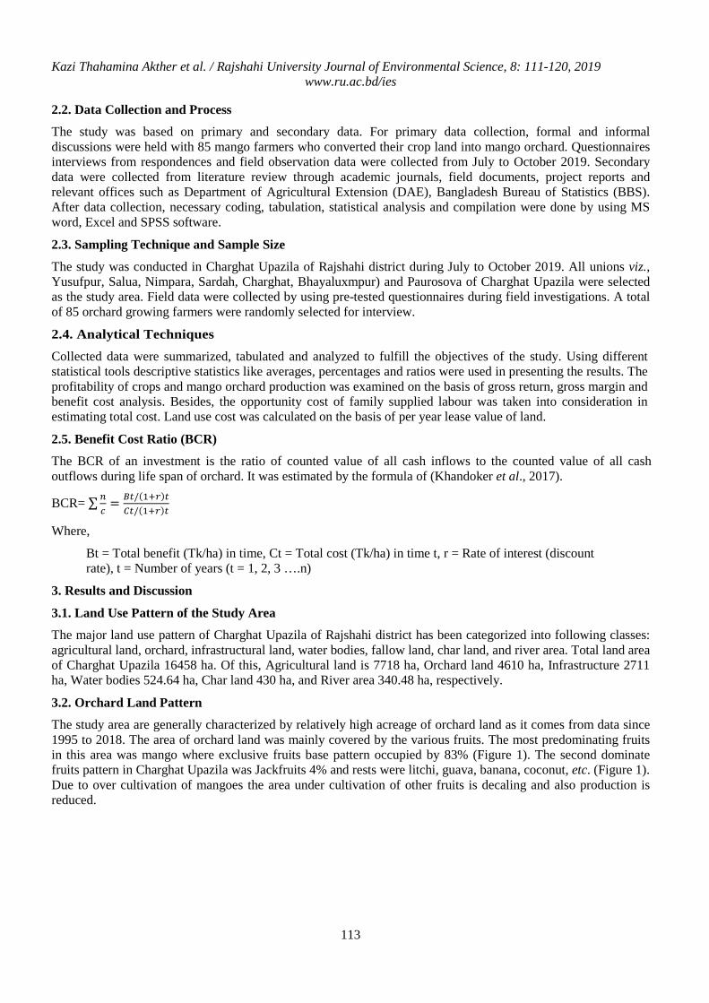
Kazi Thahamina Akther et al. / Rajshahi University Journal of Environmental Science, 8: 111-120, 2019 www.ru.ac.bd/ies
113
2.2. Data Collection and Process
The study was based on primary and secondary data. For primary data collection, formal and informal discussions were held with 85 mango farmers who converted their crop land into mango orchard. Questionnaires interviews from respondences and field observation data were collected from July to October 2019. Secondary data were collected from literature review through academic journals, field documents, project reports and relevant offices such as Department of Agricultural Extension (DAE), Bangladesh Bureau of Statistics (BBS). After data collection, necessary coding, tabulation, statistical analysis and compilation were done by using MS word, Excel and SPSS software.
2.3. Sampling Technique and Sample Size
The study was conducted in Charghat Upazila of Rajshahi district during July to October 2019. All unions viz., Yusufpur, Salua, Nimpara, Sardah, Charghat, Bhayaluxmpur) and Paurosova of Charghat Upazila were selected as the study area. Field data were collected by using pre-tested questionnaires during field investigations. A total of 85 orchard growing farmers were randomly selected for interview.
2.4. Analytical Techniques
Collected data were summarized, tabulated and analyzed to fulfill the objectives of the study. Using different statistical tools descriptive statistics like averages, percentages and ratios were used in presenting the results. The profitability of crops and mango orchard production was examined on the basis of gross return, gross margin and benefit cost analysis. Besides, the opportunity cost of family supplied labour was taken into consideration in estimating total cost. Land use cost was calculated on the basis of per year lease value of land.
2.5. Benefit Cost Ratio (BCR)
The BCR of an investment is the ratio of counted value of all cash inflows to the counted value of all cash outflows during life span of orchard. It was estimated by the formula of (Khandoker et al., 2017).
BCR= ∑𝑛𝑐
= 𝐵𝑡/(1+𝑟)𝑡𝐶𝑡/(1+𝑟)𝑡
Where,
Bt = Total benefit (Tk/ha) in time, Ct = Total cost (Tk/ha) in time t, r = Rate of interest (discount rate), t = Number of years (t = 1, 2, 3 ….n)
3. Results and Discussion
3.1. Land Use Pattern of the Study Area
The major land use pattern of Charghat Upazila of Rajshahi district has been categorized into following classes: agricultural land, orchard, infrastructural land, water bodies, fallow land, char land, and river area. Total land area of Charghat Upazila 16458 ha. Of this, Agricultural land is 7718 ha, Orchard land 4610 ha, Infrastructure 2711 ha, Water bodies 524.64 ha, Char land 430 ha, and River area 340.48 ha, respectively.
3.2. Orchard Land Pattern
The study area are generally characterized by relatively high acreage of orchard land as it comes from data since 1995 to 2018. The area of orchard land was mainly covered by the various fruits. The most predominating fruits in this area was mango where exclusive fruits base pattern occupied by 83% (Figure 1). The second dominate fruits pattern in Charghat Upazila was Jackfruits 4% and rests were litchi, guava, banana, coconut, etc. (Figure 1). Due to over cultivation of mangoes the area under cultivation of other fruits is decaling and also production is reduced.
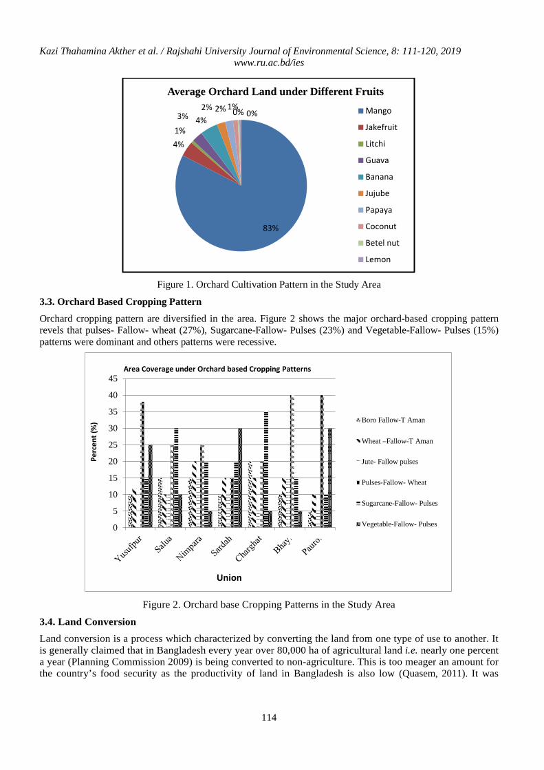
Kazi Thahamina Akther et al. / Rajshahi University Journal of Environmental Science, 8: 111-120, 2019 www.ru.ac.bd/ies
114
Figure 1. Orchard Cultivation Pattern in the Study Area
3.3. Orchard Based Cropping Pattern
Orchard cropping pattern are diversified in the area. Figure 2 shows the major orchard-based cropping pattern revels that pulses- Fallow- wheat (27%), Sugarcane-Fallow- Pulses (23%) and Vegetable-Fallow- Pulses (15%) patterns were dominant and others patterns were recessive.
Figure 2. Orchard base Cropping Patterns in the Study Area
3.4. Land Conversion
Land conversion is a process which characterized by converting the land from one type of use to another. It is generally claimed that in Bangladesh every year over 80,000 ha of agricultural land i.e. nearly one percent a year (Planning Commission 2009) is being converted to non-agriculture. This is too meager an amount for the country’s food security as the productivity of land in Bangladesh is also low (Quasem, 2011). It was
83%
4% 1%
3% 4% 2% 2% 1% 0% 0%
Average Orchard Land under Different Fruits
Mango
Jakefruit
Litchi
Guava
Banana
Jujube
Papaya
Coconut
Betel nut
Lemon
0
5
10
15
20
25
30
35
40
45
Boro Fallow-T Aman
Wheat –Fallow-T Aman
Jute- Fallow pulses
Pulses-Fallow- Wheat
Sugarcane-Fallow- Pulses
Vegetable-Fallow- Pulses
Area Coverage under Orchard based Cropping Patterns
Union
Perc
ent (
%)
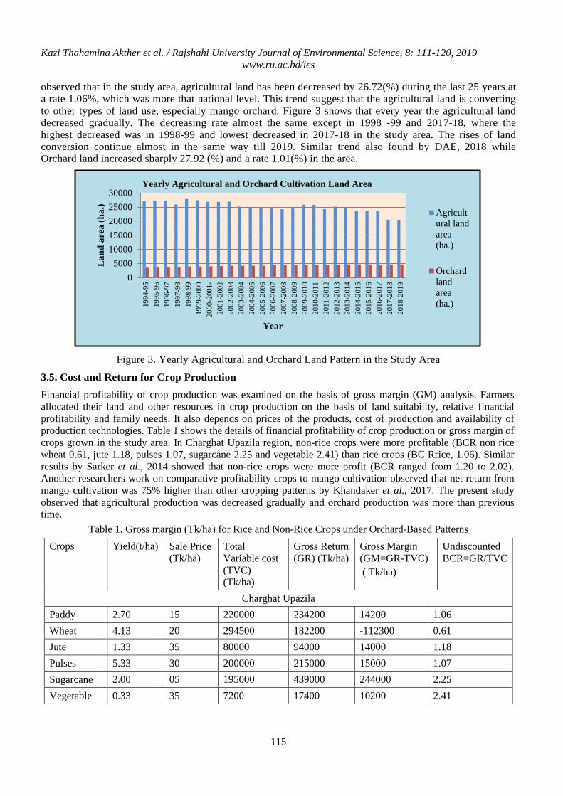
Kazi Thahamina Akther et al. / Rajshahi University Journal of Environmental Science, 8: 111-120, 2019 www.ru.ac.bd/ies
115
observed that in the study area, agricultural land has been decreased by 26.72(%) during the last 25 years at a rate 1.06%, which was more that national level. This trend suggest that the agricultural land is converting to other types of land use, especially mango orchard. Figure 3 shows that every year the agricultural land decreased gradually. The decreasing rate almost the same except in 1998 -99 and 2017-18, where the highest decreased was in 1998-99 and lowest decreased in 2017-18 in the study area. The rises of land conversion continue almost in the same way till 2019. Similar trend also found by DAE, 2018 while Orchard land increased sharply 27.92 (%) and a rate 1.01(%) in the area.
Figure 3. Yearly Agricultural and Orchard Land Pattern in the Study Area
3.5. Cost and Return for Crop Production
Financial profitability of crop production was examined on the basis of gross margin (GM) analysis. Farmers allocated their land and other resources in crop production on the basis of land suitability, relative financial profitability and family needs. It also depends on prices of the products, cost of production and availability of production technologies. Table 1 shows the details of financial profitability of crop production or gross margin of crops grown in the study area. In Charghat Upazila region, non-rice crops were more profitable (BCR non rice wheat 0.61, jute 1.18, pulses 1.07, sugarcane 2.25 and vegetable 2.41) than rice crops (BC Rrice, 1.06). Similar results by Sarker et al., 2014 showed that non-rice crops were more profit (BCR ranged from 1.20 to 2.02). Another researchers work on comparative profitability crops to mango cultivation observed that net return from mango cultivation was 75% higher than other cropping patterns by Khandaker et al., 2017. The present study observed that agricultural production was decreased gradually and orchard production was more than previous time.
Table 1. Gross margin (Tk/ha) for Rice and Non-Rice Crops under Orchard-Based Patterns Crops Yield(t/ha) Sale Price
(Tk/ha) Total Variable cost (TVC) (Tk/ha)
Gross Return (GR) (Tk/ha)
Gross Margin (GM=GR-TVC) ( Tk/ha)
Undiscounted BCR=GR/TVC
Charghat Upazila Paddy 2.70 15 220000 234200 14200 1.06 Wheat 4.13 20 294500 182200 -112300 0.61 Jute 1.33 35 80000 94000 14000 1.18 Pulses 5.33 30 200000 215000 15000 1.07 Sugarcane 2.00 05 195000 439000 244000 2.25 Vegetable 0.33 35 7200 17400 10200 2.41
05000
1000015000200002500030000
1994
-95
1995
-96
1996
-97
1997
-98
1998
-99
1999
-200
020
00-2
001-
2001
-200
220
02-2
003
2003
-200
420
04-2
005
2005
-200
620
06-2
007
2007
-200
820
08-2
009
2009
-201
020
10-2
011
2011
-201
220
12-2
013
2013
-201
420
14-2
015
2015
-201
620
16-2
017
2017
-201
820
18-2
019
Lan
d ar
ea (h
a.)
Year
Yearly Agricultural and Orchard Cultivation Land Area
Agricultural landarea(ha.)
Orchardlandarea(ha.)
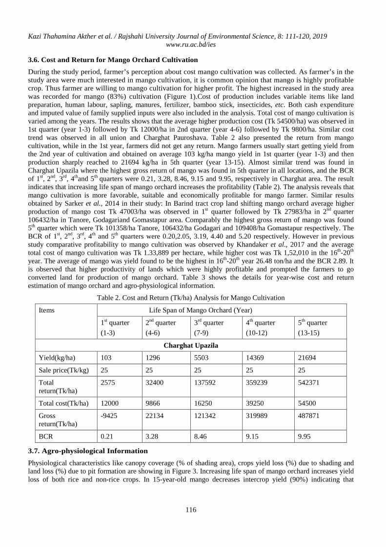
Kazi Thahamina Akther et al. / Rajshahi University Journal of Environmental Science, 8: 111-120, 2019 www.ru.ac.bd/ies
116
3.6. Cost and Return for Mango Orchard Cultivation
During the study period, farmer’s perception about cost mango cultivation was collected. As farmer’s in the study area were much interested in mango cultivation, it is common opinion that mango is highly profitable crop. Thus farmer are willing to mango cultivation for higher profit. The highest increased in the study area was recorded for mango (83%) cultivation (Figure 1).Cost of production includes variable items like land preparation, human labour, sapling, manures, fertilizer, bamboo stick, insecticides, etc. Both cash expenditure and imputed value of family supplied inputs were also included in the analysis. Total cost of mango cultivation is varied among the years. The results shows that the average higher production cost (Tk 54500/ha) was observed in 1st quarter (year 1-3) followed by Tk 12000/ha in 2nd quarter (year 4-6) followed by Tk 9800/ha. Similar cost trend was observed in all union and Charghat Pauroshava. Table 2 also presented the return from mango cultivation, while in the 1st year, farmers did not get any return. Mango farmers usually start getting yield from the 2nd year of cultivation and obtained on average 103 kg/ha mango yield in 1st quarter (year 1-3) and then production sharply reached to 21694 kg/ha in 5th quarter (year 13-15). Almost similar trend was found in Charghat Upazila where the highest gross return of mango was found in 5th quarter in all locations, and the BCR of 1st, 2nd, 3rd, 4thand 5th quarters were 0.21, 3.28, 8.46, 9.15 and 9.95, respectively in Charghat area. The result indicates that increasing life span of mango orchard increases the profitability (Table 2). The analysis reveals that mango cultivation is more favorable, suitable and economically profitable for mango farmer. Similar results obtained by Sarker et al., 2014 in their study: In Barind tract crop land shifting mango orchard average higher production of mango cost Tk 47003/ha was observed in 1st quarter followed by Tk 27983/ha in 2nd quarter 106432/ha in Tanore, Godagariand Gomastapur area. Comparably the highest gross return of mango was found 5th quarter which were Tk 101358/ha Tanore, 106432/ha Godagari and 109408/ha Gomastapur respectively. The BCR of 1st, 2nd, 3rd, 4th and 5th quarters were 0.20,2.05, 3.19, 4.40 and 5.20 respectively. However in previous study comparative profitability to mango cultivation was observed by Khandaker et al., 2017 and the average total cost of mango cultivation was Tk 1.33,889 per hectare, while higher cost was Tk 1,52,010 in the 16th-20th year. The average of mango was yield found to be the highest in 16th-20th year 26.48 ton/ha and the BCR 2.89. It is observed that higher productivity of lands which were highly profitable and prompted the farmers to go converted land for production of mango orchard. Table 3 shows the details for year-wise cost and return estimation of mango orchard and agro-physiological information.
Table 2. Cost and Return (Tk/ha) Analysis for Mango Cultivation
Items Life Span of Mango Orchard (Year)
1st quarter (1-3)
2nd quarter (4-6)
3rd quarter (7-9)
4th quarter (10-12)
5th quarter (13-15)
Charghat Upazila
Yield(kg/ha) 103 1296 5503 14369 21694
Sale price(Tk/kg) 25 25 25 25 25
Total return(Tk/ha)
2575 32400 137592 359239 542371
Total cost(Tk/ha) 12000 9866 16250 39250 54500
Gross return(Tk/ha)
-9425 22134 121342 319989 487871
BCR 0.21 3.28 8.46 9.15 9.95
3.7. Agro-physiological Information
Physiological characteristics like canopy coverage (% of shading area), crops yield loss (%) due to shading and land loss (%) due to pit formation are showing in Figure 3. Increasing life span of mango orchard increases yield loss of both rice and non-rice crops. In 15-year-old mango decreases intercrop yield (90%) indicating that
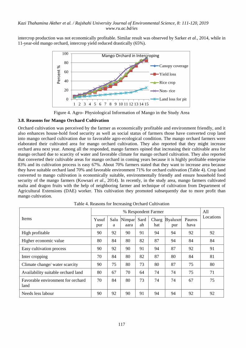
Kazi Thahamina Akther et al. / Rajshahi University Journal of Environmental Science, 8: 111-120, 2019 www.ru.ac.bd/ies
117
0
20
40
60
80
100
1 2 3 4 5 6 7 8 9 10 11 12 13 14 15
Canopy coverage
Yield loss
Rice crop
Non- rice
Land loss for pit
Mango Orchard in Intercroping Pe
rcen
t %
intercrop production was not economically profitable. Similar result was observed by Sarker et al., 2014, while in 11-year-old mango orchard, intercrop yield reduced drastically (65%).
Figure 4. Agro- Physiological Information of Mango in the Study Area
3.8. Reasons for Mango Orchard Cultivation
Orchard cultivation was perceived by the farmer as economically profitable and environment friendly, and it also enhances house-hold food security as well as social status of farmers those have converted crop land into mango orchard cultivation due to favorable agro-ecological condition. The mango orchard farmers were elaborated their cultivated area for mango orchard cultivation. They also reported that they might increase orchard area next year. Among all the responded, mango farmers opined that increasing their cultivable area for mango orchard due to scarcity of water and favorable climate for mango orchard cultivation. They also reported that converted their cultivable areas for mango orchard in coming years because it is highly profitable enterprise 83% and its cultivation process is easy 67%. About 70% farmers stated that they want to increase area because they have suitable orchard land 70% and favorable environment 71% for orchard cultivation (Table 4). Crop land converted to mango cultivation is economically suitable, environmentally friendly and ensure household food security of the mango farmers (Kowsari et al., 2014). In recently, in the study area, mango farmers cultivated malta and dragon fruits with the help of neighboring farmer and technique of cultivation from Department of Agricultural Extensions (DAE) worker. This cultivation they promoted subsequently due to more profit than mango cultivation.
Table 4. Reasons for Increasing Orchard Cultivation
Items
% Respondent Farmer All Locations Yusuf
pur Salu
a Nimpar
aara Sardah
Charghat
Byaluxmpur
Pauroshava
High profitable 90 92 90 91 94 94 92 92 Higher economic value 80 84 80 82 87 94 84 84 Easy cultivation process 90 92 90 91 94 87 92 91 Inter cropping 70 84 80 82 87 80 84 81 Climate change/ water scarcity 90 75 80 73 80 87 75 80 Availability suitable orchard land 80 67 70 64 74 74 75 71 Favorable environment for orchard land
70 84 80 73 74 74 67 75
Needs less labour 90 92 90 91 94 94 92 92
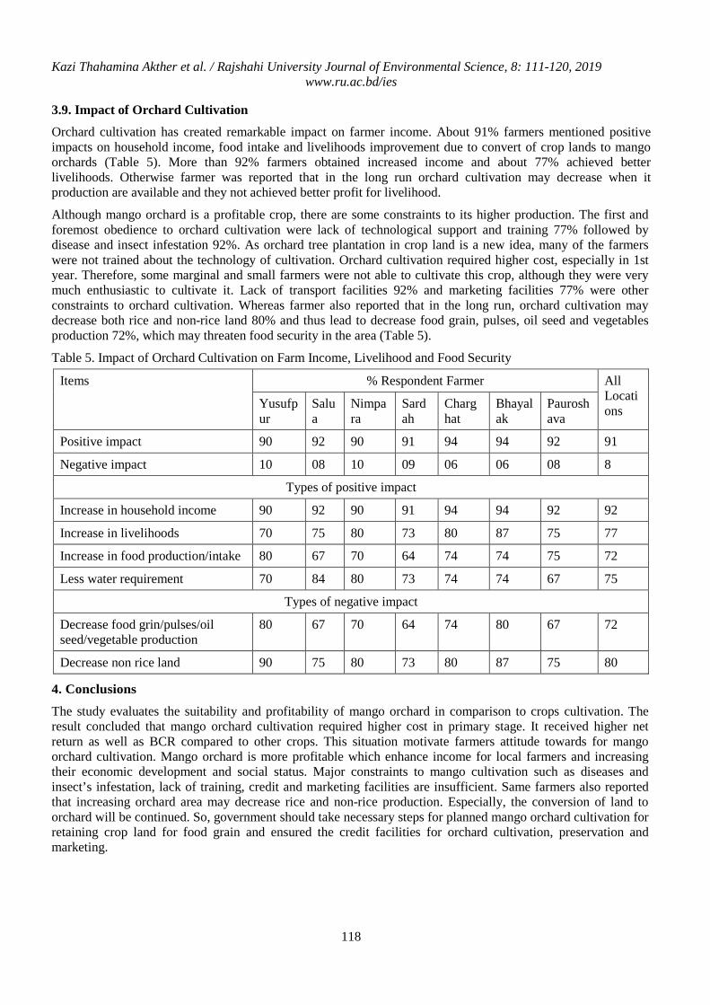
Kazi Thahamina Akther et al. / Rajshahi University Journal of Environmental Science, 8: 111-120, 2019 www.ru.ac.bd/ies
118
3.9. Impact of Orchard Cultivation
Orchard cultivation has created remarkable impact on farmer income. About 91% farmers mentioned positive impacts on household income, food intake and livelihoods improvement due to convert of crop lands to mango orchards (Table 5). More than 92% farmers obtained increased income and about 77% achieved better livelihoods. Otherwise farmer was reported that in the long run orchard cultivation may decrease when it production are available and they not achieved better profit for livelihood.
Although mango orchard is a profitable crop, there are some constraints to its higher production. The first and foremost obedience to orchard cultivation were lack of technological support and training 77% followed by disease and insect infestation 92%. As orchard tree plantation in crop land is a new idea, many of the farmers were not trained about the technology of cultivation. Orchard cultivation required higher cost, especially in 1st year. Therefore, some marginal and small farmers were not able to cultivate this crop, although they were very much enthusiastic to cultivate it. Lack of transport facilities 92% and marketing facilities 77% were other constraints to orchard cultivation. Whereas farmer also reported that in the long run, orchard cultivation may decrease both rice and non-rice land 80% and thus lead to decrease food grain, pulses, oil seed and vegetables production 72%, which may threaten food security in the area (Table 5).
Table 5. Impact of Orchard Cultivation on Farm Income, Livelihood and Food Security
Items
% Respondent Farmer All Locations Yusufp
ur Salua
Nimpara
Sardah
Charghat
Bhayalak
Pauroshava
Positive impact 90 92 90 91 94 94 92 91 Negative impact 10 08 10 09 06 06 08 8
Types of positive impact Increase in household income 90 92 90 91 94 94 92 92 Increase in livelihoods 70 75 80 73 80 87 75 77 Increase in food production/intake 80 67 70 64 74 74 75 72 Less water requirement 70 84 80 73 74 74 67 75
Types of negative impact Decrease food grin/pulses/oil seed/vegetable production
80 67 70 64 74 80 67 72
Decrease non rice land 90 75 80 73 80 87 75 80
4. Conclusions
The study evaluates the suitability and profitability of mango orchard in comparison to crops cultivation. The result concluded that mango orchard cultivation required higher cost in primary stage. It received higher net return as well as BCR compared to other crops. This situation motivate farmers attitude towards for mango orchard cultivation. Mango orchard is more profitable which enhance income for local farmers and increasing their economic development and social status. Major constraints to mango cultivation such as diseases and insect’s infestation, lack of training, credit and marketing facilities are insufficient. Same farmers also reported that increasing orchard area may decrease rice and non-rice production. Especially, the conversion of land to orchard will be continued. So, government should take necessary steps for planned mango orchard cultivation for retaining crop land for food grain and ensured the credit facilities for orchard cultivation, preservation and marketing.
Kazi Thahamina Akther et al. / Rajshahi University Journal of Environmental Science, 8: 111-120, 2019 www.ru.ac.bd/ies
119
References
Addeo G, Guastadisegni G and Pisante M. 2001. Land and water quality for sustainable and precision farming. World Congress on Conservation Agriculture, Madrid.
Banglapedia. 2019. National Encyclopedia of Bangladesh, www.banglapedia.org
Department of Agricultural Extension (DAE). 2018. Krishi Extenssion Sector Hathboi (Handbook on Agri-technology), File no-(2) Charghat Upazila, Rajshahi.
FAO (Food and Agriculture Organization). 2019. Of the UN Bangladesh Growing Source of Fruit production.
Joshi PK. 2005. Crop Diversification in India: Nature, Pattern and Drivers, National Centre for Agricultural Economics and Policyresearch, New Delhi.http://www.adb.org/Documents/Reports/Consultant/Tar-IND-4066/Agriculture/ joshi.pdf Krishna.
Kowsari MS, Miah MA and Rahman MZ. 2014. Effect of Transformation of Cropland into Mango Orchard in Selected Area of Nawabgang District. Bangladesh Journal of Extension Education, 26 (1&2): 41-47.
Khandoker S, Miah MAM, Rashid MA, Khatun M and Kundu N. 2017.Comparatively profitability analysis of shifting land from field crops to mango cultivation in selected areas of Bangladesh. Bangladesh J. Agril. Res., 42 (1):137-158.
Planning Commission. 2009. Steps Towards Change – National Strategy for Accelerated Poverty Reduction II (Revised). FY 2009-11. Government of the People’s Republic of Bangladesh, Dhaka.
Quasem MA. 2011. Conversion of Agricultural land to Non-agricultural Uses in Bangladesh: Extent and Determinant. Bangladesh Development Studies vol. XXXIV: 159-185p.
Sarker FIMGW, Biswas JC and Maniruzzaman M. 2014. Climate Change Adaptation and Economic Profitability: Crop Land Shifting to Mango Orchard in Rajshahi Region. Bangladesh Rice J., 18(1&2):18-17.
Van LWT and Keller LH. 2006. Farmers’ decision making: Perceptions of the importance, uncertainty and controllability of selected factors. Agribusiness, 7(6): 523-525.
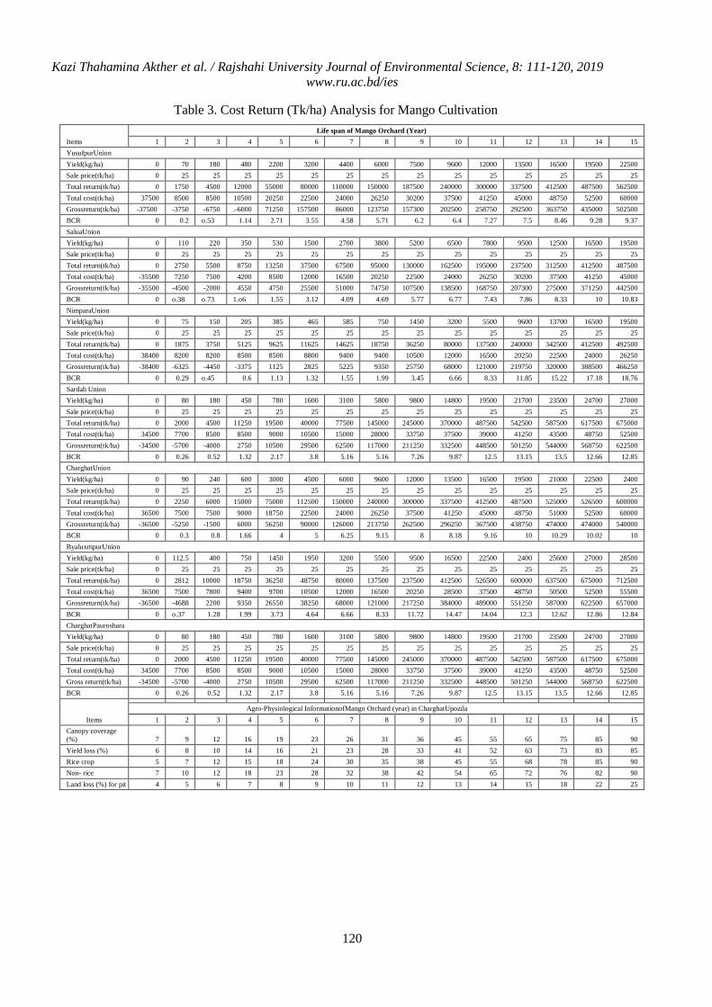
Kazi Thahamina Akther et al. / Rajshahi University Journal of Environmental Science, 8: 111-120, 2019 www.ru.ac.bd/ies
120
Table 3. Cost Return (Tk/ha) Analysis for Mango Cultivation
Items Life span of Mango Orchard (Year)
1 2 3 4 5 6 7 8 9 10 11 12 13 14 15 YusufpurUnion Yield(kg/ha) 0 70 180 480 2200 3200 4400 6000 7500 9600 12000 13500 16500 19500 22500 Sale price(tk/ha) 0 25 25 25 25 25 25 25 25 25 25 25 25 25 25 Total return(tk/ha) 0 1750 4500 12000 55000 80000 110000 150000 187500 240000 300000 337500 412500 487500 562500 Total cost(tk/ha) 37500 8500 8500 10500 20250 22500 24000 26250 30200 37500 41250 45000 48750 52500 60000 Grossreturn(tk/ha) -37500 -3750 -6750 .-6000 71250 157500 86000 123750 157300 202500 258750 292500 363750 435000 502500 BCR 0 0.2 o.53 1.14 2.71 3.55 4.58 5.71 6.2 6.4 7.27 7.5 8.46 9.28 9.37 SaluaUnion Yield(kg/ha) 0 110 220 350 530 1500 2700 3800 5200 6500 7800 9500 12500 16500 19500 Sale price(tk/ha) 0 25 25 25 25 25 25 25 25 25 25 25 25 25 25 Total return(tk/ha) 0 2750 5500 8750 13250 37500 67500 95000 130000 162500 195000 237500 312500 412500 487500 Total cost(tk/ha) -35500 7250 7500 4200 8500 12000 16500 20250 22500 24000 26250 30200 37500 41250 45000 Grossreturn(tk/ha) -35500 -4500 -2000 4550 4750 25500 51000 74750 107500 138500 168750 207300 275000 371250 442500 BCR 0 o.38 o.73 1.o6 1.55 3.12 4.09 4.69 5.77 6.77 7.43 7.86 8.33 10 10.83 NimparaUnion Yield(kg/ha) 0 75 150 205 385 465 585 750 1450 3200 5500 9600 13700 16500 19500 Sale price(tk/ha) 0 25 25 25 25 25 25 25 25 25 25 25 25 25 25 Total return(tk/ha) 0 1875 3750 5125 9625 11625 14625 18750 36250 80000 137500 240000 342500 412500 492500 Total cost(tk/ha) 38400 8200 8200 8500 8500 8800 9400 9400 10500 12000 16500 20250 22500 24000 26250 Grossreturn(tk/ha) -38400 -6325 -4450 -3375 1125 2825 5225 9350 25750 68000 121000 219750 320000 388500 466250 BCR 0 0.29 o.45 0.6 1.13 1.32 1.55 1.99 3.45 6.66 8.33 11.85 15.22 17.18 18.76 Sardah Union Yield(kg/ha) 0 80 180 450 780 1600 3100 5800 9800 14800 19500 21700 23500 24700 27000 Sale price(tk/ha) 0 25 25 25 25 25 25 25 25 25 25 25 25 25 25 Total return(tk/ha) 0 2000 4500 11250 19500 40000 77500 145000 245000 370000 487500 542500 587500 617500 675000 Total cost(tk/ha) 34500 7700 8500 8500 9000 10500 15000 28000 33750 37500 39000 41250 43500 48750 52500 Grossreturn(tk/ha) -34500 -5700 -4000 2750 10500 29500 62500 117000 211250 332500 448500 501250 544000 568750 622500 BCR 0 0.26 0.52 1.32 2.17 3.8 5.16 5.16 7.26 9.87 12.5 13.15 13.5 12.66 12.85 CharghatUnion Yield(kg/ha) 0 90 240 600 3000 4500 6000 9600 12000 13500 16500 19500 21000 22500 2400 Sale price(tk/ha) 0 25 25 25 25 25 25 25 25 25 25 25 25 25 25 Total return(tk/ha) 0 2250 6000 15000 75000 112500 150000 240000 300000 337500 412500 487500 525000 526500 600000 Total cost(tk/ha) 36500 7500 7500 9000 18750 22500 24000 26250 37500 41250 45000 48750 51000 52500 60000 Grossreturn(tk/ha) -36500 -5250 -1500 6000 56250 90000 126000 213750 262500 296250 367500 438750 474000 474000 540000 BCR 0 0.3 0.8 1.66 4 5 6.25 9.15 8 8.18 9.16 10 10.29 10.02 10 ByaluxmpurUnion Yield(kg/ha) 0 112.5 400 750 1450 1950 3200 5500 9500 16500 22500 2400 25600 27000 28500 Sale price(tk/ha) 0 25 25 25 25 25 25 25 25 25 25 25 25 25 25 Total return(tk/ha) 0 2812 10000 18750 36250 48750 80000 137500 237500 412500 526500 600000 637500 675000 712500 Total cost(tk/ha) 36500 7500 7800 9400 9700 10500 12000 16500 20250 28500 37500 48750 50500 52500 55500 Grossreturn(tk/ha) -36500 -4688 2200 9350 26550 38250 68000 121000 217250 384000 489000 551250 587000 622500 657000 BCR 0 o.37 1.28 1.99 3.73 4.64 6.66 8.33 11.72 14.47 14.04 12.3 12.62 12.86 12.84 CharghatPauroshara Yield(kg/ha) 0 80 180 450 780 1600 3100 5800 9800 14800 19500 21700 23500 24700 27000 Sale price(tk/ha) 0 25 25 25 25 25 25 25 25 25 25 25 25 25 25 Total return(tk/ha) 0 2000 4500 11250 19500 40000 77500 145000 245000 370000 487500 542500 587500 617500 675000 Total cost(tk/ha) 34500 7700 8500 8500 9000 10500 15000 28000 33750 37500 39000 41250 43500 48750 52500 Gross return(tk/ha) -34500 -5700 -4000 2750 10500 29500 62500 117000 211250 332500 448500 501250 544000 568750 622500 BCR 0 0.26 0.52 1.32 2.17 3.8 5.16 5.16 7.26 9.87 12.5 13.15 13.5 12.66 12.85
Items
Agro-Physiological InformationofMango Orchard (year) in CharghatUpozila 1 2 3 4 5 6 7 8 9 10 11 12 13 14 15
Canopy coverage (%) 7 9 12 16 19 23 26 31 36 45 55 65 75 85 90 Yield loss (%) 6 8 10 14 16 21 23 28 33 41 52 63 73 83 85 Rice crop 5 7 12 15 18 24 30 35 38 45 55 68 78 85 90 Non- rice 7 10 12 18 23 28 32 38 42 54 65 72 76 82 90 Land loss (%) for pit 4 5 6 7 8 9 10 11 12 13 14 15 18 22 25
Meherun Nesa et al. / Rajshahi University Journal of Environmental Science, 8: 121-126, 2019 www.ru.ac.bd/ies
Potentiation of Burmese Pink Cassia Cassia renigera Benth Extracts against Brine Shrimp Nauplii Artemia salina (L.) and Lymnaea acuminata Lamarck
Meherun Nesa, Sahadat Hossain, Sadia Afrin Rimi and Nurul Islam∗
Department of Zoology, University of Rajshahi, Rajshahi-6205, Bangladesh.
Abstract
Pet. (Petroleum) ether, CHCl3 (Chloroform) and CH3OH (Methanol) extracts of leaves and stem-bark of Cassia renigera Benth. were evaluated against brine shrimp Artemia salina (L.) nauplii and Lymnaea acuminata Lamarck adults through cytotoxicity and molluscicidal activity tests. Except the Pet. ether extract of leaves all the rest were found effective. Against A. salina nauplii the C. renigera leaves gave LC50 values 428.54, 315.20, 240.30, 180.20, 163.22 and 126.54 ppm for the CHCl3 extract and 528.90, 358.21, 270.70, 192.56, 195.63 and 140.20 ppm for the CH3OH extract after 18, 24, 30, 36, 42 and 48 h of exposure respectively. The stem bark gave LC50 values 536.23, 339.43, 271.56, 192.56, 186.58 and 140.20 ppm for Pet. ether extract; 662.82, 368.90, 283.48, 205.04, 189.97 and 156.85 ppm for CHCl3 and 551.60, 368.90, 334.24, 233.07, 215.52 and 140.22 ppm for CH3OH extract, all after 18, 24, 30, 36, 42 and 48 h of exposure respectively. Against L. acuminata the C. renigera leaves gave LC50 values 117.15, 103.30, 91.65, 66.74, 66.74, 52.12 and 49.35 ppm for the CHCl3 extract, and 216.04, 177.94, 149.50, 111.61, 92.34, 59.43 and 52.20 ppm for the CH3OH extract; the stem bark gave LC50 values 105.77, 140.07, 100.62, 95.48, 86.76, 71.47 and 66.40 ppm; 129.37, 111.72, 96.67, 85.28, 77.66, 78.82 and 77.70 ppm, and 134.76, 107.35, 102.26, 94.21, 83.25, 80.70 and 77.00 ppm for Pet. ether, CHCl3 and CH3OH extracts after 12, 18, 24, 30, 36, 42 and 48 h of exposure respectively.
Keywords: Potentiation; Cassia renigera; Extracts; Artemia salina; Lymnaea acuminata.
1. Introduction
Cassia renigera Benth belongs to the Family- Caesalpinaceae. It mainly grows throughout the tropical countries. It is commonly known as Burmese Pink Cassia. The genus Cassia consists of nearly 1000 species and C. renigera is one of the remarkable species among them (Rahman, 2013; Jain and De Filipps, 1991). It is a small tree less than 20 feet in height. In May, when the large, impressive flowers, as well as green leaves and tenders appear, it looks like an amazingly gorgeous picture, heightened by the varied characters of pink in each of the clusters (Pawar and Mello, 2011). In traditional medicine, numerous medicinal properties of C. renigera have been recognized from time to time. Among them, sennosides are well known to the people for having remarkable medicinal values (Raghunathan et al., 1974). Extracts of different Cassia species have been used as remedy for rheumatic disease, skin ailments and as laxatives (De Filipps, 1991; Hooker, 1879; Bhakta et al., 1999). The leaf and seed extracts have been found to possess significant hepatoprotective activity and anti-inflammatory activity (Hossain et al., 2018; Nesa et al., 2017; Yadav et al., 2013; Maity and Dinda, 2003; Asolkar, 1992). Previously, the plant has been examined for identifying its antifeedant, larvicidal, antioxidant, antitumour, anti-inflammatory and antimicrobial activities against different test agents (Gupta, 2000; Luximon-Ramma et al., 2002; Raju et al., 2005; Aneja et al., 2011; Duraipandiyan et al., 2011). High potential mortality has been recorded against different stored grain pests and also found to be proficient in controlling grain damages and seed weight loss (Weaver and Subramanyam, 2000; Sabbour, et al., 2007). Many synthetic pesticides have been introduced in the recent time to control agricultural, veterinary, medical and household insect pests. But due to the voluminous and iterative use of synthetic pesticides have attributed so many pernicious effects on the environment and also occur intoxication to non-target organisms (Gupta et al., 2001). So, at present special emphasize has been given to the probable use of botanicals or plant products as promising substitutes to chemical insecticides in controlling insect pests (Khalequzzaman and Islam, 1992; Ohazurike et al., 2003; Umoetok and Gerard, 2003; Abdelouaheb et al., 2009). This intimation has created a worldwide interest in the development of alternative recipe, including the
Meherun Nesa et al. / Rajshahi University Journal of Environmental Science, 8: 121-126, 2019 www.ru.ac.bd/ies
122
discovery of fresher insecticides (Dayan et al., 2009). In this investigation, leaves and stem-barks of the plant C. renigera have been taken into consideration to find out the cytotoxic effects against Artemia salina and molluscicidal activity against Lymnaea acuminata.
2. Materials and Methods
2.1. Collection and Preparation of Test Materials
Fresh leaves and stem-barks of the Burmese Pink Cassia C. renigera were collected separately from the Botanical Garden of the University of Rajshahi, Bangladesh. Identification of the target plant was confirmed by the experts on plant taxonomy in the Department of Botany, University of Rajshahi, Bangladesh. Collected plant materials were cleaned properly with the help of a brush and sliced into small pieces. The chips were spread out on wooden-tray to dry. This was done at room temperature under shade avoiding direct sunshine. The materials were rearranged thrice daily to avoid heaping. It needed 10 to 15 days to ready for grinding. Then the plant materials were powdered in an electric grinder machine avoiding additional heat during grinding. The ground materials were placed separately into conical flasks to add solvents in a proportion of 10:1 as solvent and plant dust materials sealed in conical flask (250 ml) to keep on a shaker for 48 h. The Pet. ether, CHCl3 and CH3OH (Merck, Germany) were used (200 g × 600 mL × 2 times) successively while each of which kept 48 h on a shaker. For each of the extracts filtration was done by using filter paper at 24 h interval in the same flask followed by evaporation until the extract was left as a scum. The extracts were removed to glass vials and preserved in a refrigerator at 4°C with proper labeling.
2.2. Collection and Culture of Test Insects
The test agent Artemia salina nauplii were emerged from the cysts released in a beaker containing salty water. The nauplii were hatched from the cysts within a period of 24h of age. Another test agent, adult snails of Lymnaea acuminata were collected from the nearby ponds and low-lying submerged areas in the Rajshahi University Campus. The collected snails were reared in pond water in an aquarium under laboratory conditions for the continuous supply of snails of same size and age during experimentation.
2.3. Brine Shrimp Lethality Test
First of all, the test tubes were filled with 10 ml of water and marked the lower meniscus with a marker pen and the tubes were made empty. Then, the doses were prepared at five different concentrations in the test tubes by adding a calculated amount of DMSO (dimethylsulfoxide) with the extracts in order to make them hydrophilic prior to add half of the required amount of water in each. The nauplii were counted by visual inspection and were released in each of the test-tubes with the help of a pipette; the additional amount of water was added to fill the test tubes up to the pre-marked level containing 10 ml of water including the test-tube considered as a control batch. Observation of mortality was made after 18, 24, 30, 36, 42 and 48 h of exposure. Doses for all three extracts (Pet. ether, CHCl3 and CH3OH) were 200, 400 and 600 ppm, respectively.
2.4. Molluscicidal Activity Test
From the aquarium culture adult L. acuminata snails were collected. In each of the 50 ml beakers ten individuals were kept. Test samples at different concentrations considered as doses were prepared in beakers by adding calculated amount of DMSO (Dimethylsulfoxide) to make them hydrophilic before adding half of the required amount of water in each. After that a certain amount of pond water was added to fill up the pre-marked beakers with the help of a pipette. The snails were counted by visual inspection and were released in the beakers containing 10 ml of water. Observation of mortality was made after 12, 18, 24, 30, 36, 42 and 48 h of exposure with an interval of 6 h. After experimenting pilot doses, the final applicable doses for leaf extracts were fixed as 50, 60 and 70 ppm; for stem-bark extracts the fixed doses were 70, 80 and 90 ppm. All the experiments were carried out in the Crop Protection & Toxicology Laboratory of the Department of Zoology, University of Rajshahi, Rajshahi-6205, Bangladesh.
2.5. Statistical Analysis
The mortality (%) was corrected using Abbott’s formula (Abbott, 1925). The data were then subjected to Probit analysis by using GW Basic software (Busvine, 1971; Finney, 1947).
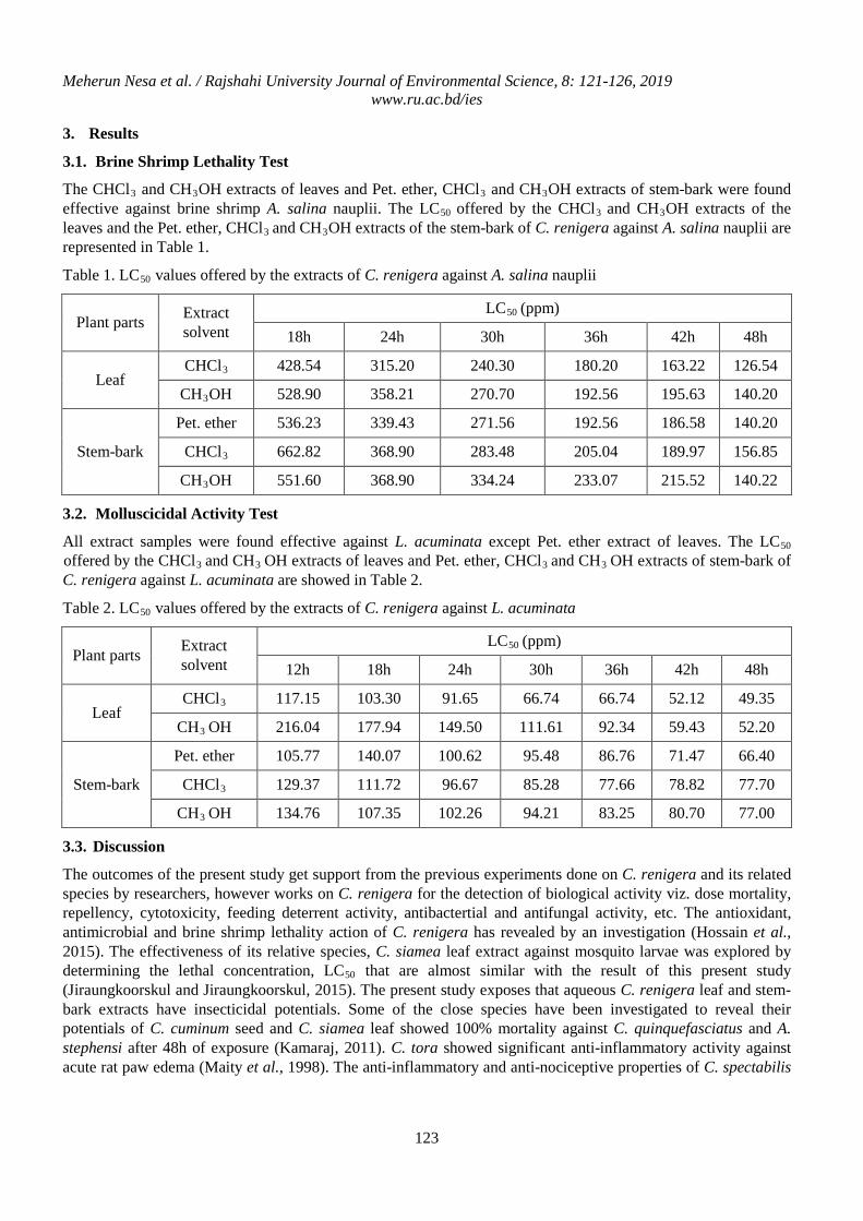
Meherun Nesa et al. / Rajshahi University Journal of Environmental Science, 8: 121-126, 2019 www.ru.ac.bd/ies
123
3. Results
3.1. Brine Shrimp Lethality Test
The CHCl3 and CH3OH extracts of leaves and Pet. ether, CHCl3 and CH3OH extracts of stem-bark were found effective against brine shrimp A. salina nauplii. The LC50 offered by the CHCl3 and CH3OH extracts of the leaves and the Pet. ether, CHCl3 and CH3OH extracts of the stem-bark of C. renigera against A. salina nauplii are represented in Table 1.
Table 1. LC50 values offered by the extracts of C. renigera against A. salina nauplii
Plant parts Extract solvent
LC50 (ppm) 18h 24h 30h 36h 42h 48h
Leaf CHCl3 428.54 315.20 240.30 180.20 163.22 126.54
CH3OH 528.90 358.21 270.70 192.56 195.63 140.20
Stem-bark Pet. ether 536.23 339.43 271.56 192.56 186.58 140.20
CHCl3 662.82 368.90 283.48 205.04 189.97 156.85 CH3OH 551.60 368.90 334.24 233.07 215.52 140.22
3.2. Molluscicidal Activity Test
All extract samples were found effective against L. acuminata except Pet. ether extract of leaves. The LC50
offered by the CHCl3 and CH3 OH extracts of leaves and Pet. ether, CHCl3 and CH3 OH extracts of stem-bark of C. renigera against L. acuminata are showed in Table 2.
Table 2. LC50 values offered by the extracts of C. renigera against L. acuminata
Plant parts Extract solvent
LC50 (ppm) 12h 18h 24h 30h 36h 42h 48h
Leaf CHCl3 117.15 103.30 91.65 66.74 66.74 52.12 49.35
CH3 OH 216.04 177.94 149.50 111.61 92.34 59.43 52.20
Stem-bark Pet. ether 105.77 140.07 100.62 95.48 86.76 71.47 66.40
CHCl3 129.37 111.72 96.67 85.28 77.66 78.82 77.70 CH3 OH 134.76 107.35 102.26 94.21 83.25 80.70 77.00
3.3. Discussion
The outcomes of the present study get support from the previous experiments done on C. renigera and its related species by researchers, however works on C. renigera for the detection of biological activity viz. dose mortality, repellency, cytotoxicity, feeding deterrent activity, antibactertial and antifungal activity, etc. The antioxidant, antimicrobial and brine shrimp lethality action of C. renigera has revealed by an investigation (Hossain et al., 2015). The effectiveness of its relative species, C. siamea leaf extract against mosquito larvae was explored by determining the lethal concentration, LC50 that are almost similar with the result of this present study (Jiraungkoorskul and Jiraungkoorskul, 2015). The present study exposes that aqueous C. renigera leaf and stem-bark extracts have insecticidal potentials. Some of the close species have been investigated to reveal their potentials of C. cuminum seed and C. siamea leaf showed 100% mortality against C. quinquefasciatus and A. stephensi after 48h of exposure (Kamaraj, 2011). C. tora showed significant anti-inflammatory activity against acute rat paw edema (Maity et al., 1998). The anti-inflammatory and anti-nociceptive properties of C. spectabilis
Meherun Nesa et al. / Rajshahi University Journal of Environmental Science, 8: 121-126, 2019 www.ru.ac.bd/ies
124
were assessed by an investigation (Da Silva et al., 2012). C. auriculata extract exposed antioxidant properties both in vitro and in vivo conditions (Juan-Badaturuge et al., 2011; Rajagopal et al., 2003). Additional studies discovered that the C. auriculata, a relative species of C. renigera, have antihyperlipidemic effect (Gupta et al., 2009; Gupta et al., 2011).
4. Conclusion
After analyzing the results of this investigation and considering the outcome the previous works done on C. renigera and its relative species, it could be concluded that further developments on the secondary metabolites of this could be used in the pest control strategy. Further investigation should be taken into consideration to explore the exact compound for which this plant extracts show pesticidal effect.
References
Abbott WS. 1925. A method of computing the effectiveness of an insecticide. J. Econ. Ent., 18(2):265-267.
Abdelouaheb A, Nassima R and Noureddine S. 2009. Larvicidal activity of a neem tree extract (Azadirachtin) against mosquito larvae in the Republic of Algeria. Jordan J. Biol. Sci., 2(1):15-22.
Aneja R, Sharma C and Joshi R. 2011. In vitro efficacy of amaltas (Cassia fistula L.) against the pathogens causing otitis externa. Jundishapur J. Microbiol., 4(3):175-183.
Asolkar LV, Kakkar KK and Chakre OJ. 1992. Second Supplement to Glossary of Indian Medicinal Plants. 11th Ed. (PID, CSIR, New Delhi) 80 pp.
Bhakta T, Mukherjee PK, Mukherjee K, Banerjee S, Mandal SC, Maity TK, Pal M and Saha BP. 1999. Evaluation of hepatoprotective activity of Cassia fistula leaf extract. J. Ethanopharmacol., 66(3):277-282.
Busvine JR. 1971. A critical review of the techniques for testing insecticides. Commonwealth Agricultural Buereux, London. 345 pp.
Da Silva KA, Manjavachi MN, Paszcuk AF, Pivatto M, Viegas C Jr, Bolzani VS and Calixto JB. 2012. Plant derived alkaloid (-)-cassine induces anti-inflammatory and anti-hyperalgesics effects in both acute and chronic inflammatory and neuropathic pain models. Neuropharmacol., 62:967-977.
Dayan FE, Cantrell CL and Duke SO. 2009. Natural products in crop protection. Bioorg. Med. Chem., 17(12):4022-4034.
Duraipandiyan V, Ignacimuthu S and Gabriel PM. 2011. Antifeedant and larvicidal activities of Rhein isolated from the flowers of Cassia fistula L. Saudi J. Biol. Sci., 18(2):129-133.
Finney DJ. 1947. Probit analysis: a statistical treatment of the sigmoid response curve, Cambridge University Press. London. 333 pp.
Gupta A, Upadhyay RK and Saxena PN. 2001. Toxicity evaluation of certain blood biochemical parameters in Passer domesticus (Linn.). J. Scientif. Industr. Res., 60:668-674.
Gupta M, Mazumder UK, Rath N and Mukhopadhyay DK. 2000. Antitumor activity of methanolic extract of Cassia fistula L. seed against Ehrlich ascites carcinoma. J. Ethnopharmacol.,72(1-2):151-156.
Gupta S, Sharma SB, Prabhu KM, Bansal SK. 2009. Protective role of Cassia auriculata leaf extract on hyperglycemia-induced oxidative stress and its safety evaluation. Indian J. Biochem. Biophys., 46:371-377.
Gupta S, Sharma SB, Singh UR and Bansal SK. 2011. Salutary Effect of Cassia auriculata L. leaves on hyperglycemia-induced atherosclerotic environment in streptozotocin rats. Cardiovasc. Toxicol., 11(4):308-315.
Hooker JD. 1879. The Flora of British India, Vol. II, L. (Reeve and Co., England) 26 pp.
Meherun Nesa et al. / Rajshahi University Journal of Environmental Science, 8: 121-126, 2019 www.ru.ac.bd/ies
125
Hossain MM, Mondal M, Hossain MP, Uddin MS, Uddin N, Hasan MM, Hossain MS, Islam AFMM, Rana MS. 2015. In vitro antioxidant, brine shrimp lethality and antimicrobial activities of methanol and petroleum ether extracts of Cassia renigera fruit. J Food Measurement Characterization. 9(1):68-75. https: //doi.org/ 10.1007/ s11694-014-9211
Hossain MM, Mondal M, Morad RU, Uddin N, Das A, Hossain MS, Kamal MM, Islam MF, Wahed TB and Chowdhury MMH, 2018. Evaluation of bioactivities of methanol and petroleum ether extracts of Cassia renigera seed. Clinical Phytosci., 4: Article No. 33.
Jain SK and De Filipps RA. 1991. Medicinal plants of India. Reference Publ. Inc., Michigan. 849 pp.
Jiraungkoorskul K and Jiraungkoorskul W. 2015. Larvicidal and histopathological effects of Cassia siamea leaf extract against Culex quinquefasciatus. Trop. Life Sci. Res., 26(2):15-25.
Juan-Badaturuge M, Habtemariam S and Thomas MJK. 2011. Antioxidant compounds from a South Asian beverage and medicinal plant, Cassia auriculata. Food Chem., 125:221-225.
Kamaraj C, Rahuman AA, Bagavan A, Elango G, Zahir AA and Santhoshkumar T. 2011. Larvicidal and repellent activity of medicinal plant extracts from Eastern Ghats of South India against malaria and filariasis vectors. Asian Pac. J. Trop. Med., 4(9):698-705.
Khalequzzaman M and Islam MN. 1992. Pesticidal action of Dhatura, Datura metel Linn. leaf extracts on Tribolium castaneum (Herbst). Bangladesh J. Zool., 20(2):223-229.
Luximon-Ramma, Behorun T, Soobrattee MA and Aruoma OI. 2002. Antioxidant activities of phenolic, proanthocyanidin, and flavonoid components in extracts of Cassia fistula. J. Agric. Food Chem., 50(18):5042-5047.
Maity TK and Dinda SC. 2003. Purgative activity of Cassia tora Leaf extract and isolated Aloe-Emodin, Indian J. Pharm. Sci., 65(1):93-95.
Maity TK, Mandal SC, Mukherjee PK, Saha K, Das J, Pal M and Saha BP, 1998. Studies on antiinflammatory effect of Cassia tora leaf extract (Fam. Leguminosae). Phytother. Res., 12:221–223.
Nesa M, Islam S, Sharma SK, Rekha SB, Ferdous J and Islam N, 2017. Bioactive Potentials of Cassia renigera Benth. Extracts Against the Stored Product Pests Callosobruchus chinensis L., Sitophilus oryzae L. and Tribolium castaneum (Hbst.), J. Sci. Res., 9 (4), 351-357; www.banglajol.info/index.php/JSR
Ohazurike NC, Omuh MO and Emeribe EO. 2003. The use of seed extracts of the physic nut (Jatropha curcas L.) in the control of maize weevil (Sitophilus zeamais M.) in stored maize grains (Zea mays L.). Global J. Agric. Sci., 2:86-88.
Pawar HA and Mello PMD. 2011. Cassia tora Linn.: An Overview. Int. J. Pharma. Sci. Res., 2(9):2286-2291.
Raghunathan K, Hariharan V and Rangaswami S. 1974. Chrysophanol-1-β-gentiobioside, a new anthraquinone glycoside from Cassia tora Linn. Indian J. Chem. 12:1251-1253.
Rahman AHMM. 2013. Angiospermic Flora of Rajshahi District, Bangladesh. American J. Life Sci., 1(3):105-112.
Rajagopal SK, Manickam P, Periyasamy V and Namasivayam N. 2003. Activity of Cassia auriculata leaf extract in rats with alcoholic liver injury. J. Nutri. Biochem., 14:452-458.
Raju I, Moni M and Subramanian V. 2005. Anti-inflammatory and antioxidant activities of Cassia fistula Linn bark extract. African J. Traditional Comple. Alternat. Med., 2(1):70-85.
Sabbour MM, Shadia E and Abd-Al-Aziz. 2007. Efficiency of some bioinsecticides against broad bean beetle, Bruchus rufimanus (Coleoptera : Bruchidae ). Res. J. Agric. Biol. Sci., 3(2):67-72.

Meherun Nesa et al. / Rajshahi University Journal of Environmental Science, 8: 121-126, 2019 www.ru.ac.bd/ies
126
Umoetok SBA and Gerard MB. 2003. Comparative efficacy of Acorus calamus powder and two synthetic insecticides for control of three major insect pests of stored cereal grains. Global J. Agric. Sci., 2:94-97.
Weaver DK and Subramanyam B. 2000. Botanicals. In: Subramanyam, B., Hagstrum, D.W. (Eds.), Alternatives to Pesticides in Stored-Product IPM. Kluwer Academic Publishers, Massachusetts, USA, 303–320.
Yadav A, Bhardwaj R and Sharma RA, 2013. Phytochemical Screening and Antimicrobial Activity of Anthraquinones Isolated from Different Parts of Cassia nodosa. Res. J. Med. Plants., 7(3): 150-157. DOI: 10.3923/rjmp.2013.150.157.
Nayeema Parvin et al. / Rajshahi University Journal of Environmental Science, 8: 127-134, 2019 www.ru.ac.bd/ies
Vector Control Potentials of Mentha piperita L.
Nayeema Parvin1, H.S. Jahidul Ferdous2 and Nurul Islam3∗
1Institute of Environmental Science, University of Rajshahi, Rajshahi 6205, Bangladesh 2Bangladesh Agriculture Development Corporation (BADC), Government of the People’s Republic of Bangladesh
*3Department of Zoology, University of Rajshahi, Rajshahi 6205, Bangladesh
Abstract The whole plant (wp) of Mentha piperita L. was extracted in petroleum ether (Pet. ether), chloroform (CHCl3) and methanol (CH3OH), and were screened through dose-mortality and repellency tests against eggplant aphid, Aphis gossypii and only dose-mortality assay against larvae of the mosquito, Culexquinque fasciatus under laboratory conditions. Against A. gossypii for Pet. ether extract the LD50 values were 0.235, 0.189, 0.158, 0.136, 0.111, 0.093, 0.083 and 0.070 mg cm-2; for CHCl3 0.252, 0.198, 0.189, 0.156, 0.130, 0.107, 0.103 and 0.095 mg cm-2; and for CH3 OH extracts 0.412, 0.332, 0.345, 0.328, 0.258, 0.208, 0.156 and 0.126mg cm-2 at different exposure hours. Against A. gossypii the CHCl3 and CH3 OH extracts offered repellent activity at 5% (P<0.05) and 1% (P<0.01) level of significance, while the Pet. ether extract of the same did not show repellency for aphids. In the 2nd dose-mortality assay of the same extracts one day old mosquito larvae also responded to the same extracts giving LD50 values 174.072, 114.399, 79.776, 60.519 and 46.065 ppm for Pet. ether extract, 418.844, 229.226, 183.390, 130.911 and 97.375 ppm for CHCl3 extract, and 1195.342, 1075.135, 696.966, 516.804 and 309.859 ppm for CH3 OH all for 6, 12, 18, 24 and 30h of exposures respectively. The analysis of data revealed that the test plant M. piperita possesses vector control potentials since the test agents are all vectors.
Keywords: Mentha piperita; dose-mortality; repellency; larvicidal activity; Aphis gossypii; Culexquinque fasciatus larvae
1. Introduction
First warning signals about pesticides’ danger appeared in 1962 (Carson, 1962), an American courageous woman and scientist, wrote down her nature observation and pointed out sudden dying of birds caused by indiscriminate spraying of pesticides (DDT, half-life of it in soil ranges from 22 to 30 years). Her book, Silent Spring, became a landmark. It changed the existing view on pesticides and has stimulated public concern on pesticides and their impact on health and the environment. Pesticides represent the only group of chemicals that are purposely applied to the environment with an aim to suppress pests of plants and animals and to protect agricultural and industrial products. However, the majority of pesticides are not specifically targeting the pests, they also affect non-target organisms. Thus, repeated application of pesticides leads to loss of biodiversity (Pesticide Action Network, 2010). The use of pesticides by Bangladeshi farmers increased by 328 percent during the past 10 years, posing a serious health hazards on human being due to its long-term residual effect, according to a study released by Bangladesh Rice Research Institute (Islam, 2010). The extensive use of synthetic inorganic insecticides have resulted in environmental hazards. Vector is an organism, often an invertebrate arthropod that transmits a pathogen from reservoir to host. Viruses that are transmitted between vertebrate or plant hosts by feeding insects (vectors) can replicate within both their host and their vector. Plant viruses pose some of the most severe threats to world agriculture. Because they invade the crop’s cells and cloak themselves with the plant’s normal life processes. More than half of the nearly 550 vector-transmitted virus species recorded so far are disseminated by aphids 55% and by beetles 11% (Astier et al., 2001). Aphid or plant louse is a tiny, usually green, soft-bodied, pear-shaped insect injurious to vegetation. They vary in length from 1 to 10 millimeters. Aphids feed themselves through sucking mouthparts called stylets. Some are wingless, others have two pairs of transparent or colored wings.
Mosquitoes are important vector responsible for the pathogens of various diseases like malaria, filariasis, Japanese encephalitis (JE), dengue and dengue haemorrhagic fever, yellow fever, etc. There are four common groups of mosquitoes living in the Bay Area. They are Aedes, Anopheles, Culex, and Culiseta. The mosquitoes are a family of the Culicidae. Although a few species are harmless or even useful to humanity, most are
Nayeema Parvin et al. / Rajshahi University Journal of Environmental Science, 8: 127-134, 2019 www.ru.ac.bd/ies
128
considered nuisance because they consume blood from living vertebrates, including humans. Some authorities argue accordingly that mosquitoes are the most dangerous animals on Earth (Michigan Mosquito Control Organization, 2013).
Plant is a natural source for providing mankind various secondary metabolites with antiviral or vector control activity, which are organic compounds. The present investigation was carried out to find out the vector control potential of Mentha piperita L (=Convolvulus nummularius L.), against the eggplant aphids and Culex quinque fasciatus larvae. It is a perennial herb with prostrate stem, often pilose at the nodes with short tricomes to glabrate. It binds the ground while creeping around (Ahmed et al., 2009). The whole plant is used as a medicine for hysteria, to cure burns, cuts, wounds and scropion stings (Jain, 1991). In Nepal, the paste of the plant is used to treat scabies (Manandhar, 2002). This plant can be seen on the hill slopes, edges of fields, roadsides and railway embankments. It is widely distributed in India, Nepal, Bhutan, tropical America and Africa. In Bangladesh, it is found in all districts. This medicinal plant was targeted for biological activities by many previous researches detected antioxidant activity (Haydari et al., 2019), biological activity (Alexa et al., 2018; Brahmi et al., 2017), antibacterial and antifungal activity (Al-Rajab et al., 2018; Giri et al., 2007; Gökalpİşcan et al., 2002), antibacterial and antioxidental activity (Singh et al., 2015). It also improved their biological activity of elevated CO2 induced metabolic change in basil (Jaouni et al., 2018).
2. Materials and Methods
2.1. Collection and Preparation of Test Materials
M. piperita was collected from the Rajshahi University campus, identified and kept in the herbarium of the Department of Botany, University of Rajshahi. The plants were chopped into small pieces, dried under shade and powdered using a hand grinder, weighed and placed in separate conical flasks to add Pet. ether, CHCl3 and CH3OH (Merck, Germany) (100 gm × 300 ml × 2 times) for 48 h. Filtration was done by Whatman filter paper (made in USA) at 24h interval in the same flask followed by evaporation until the extract was left. The extracts was then removed to glass vials and preserved in a refrigerator at 4○C with proper labeling.
2.2. Collection and Culture of Test Insect
Aphids are highly reproducing insects. At first some mature aphids were collected from affected plants and then released on the new fresh eggplants for further production. They multiply in a good number within a short time. Aphids were collected repeatedly from the culture field with a fine camel hair-brush in a Petri dish and used in the experiments. Mosquito eggs were hatched in stagnant water. They are collected from damp drains with special collecting spoon. Collected mosquito egg-rafts were placed into a new beaker containing pond water and kept it in a dark place inside the lab for hatching. After 24 h, hatched larvae were collected from the hatching tank and used in the experiment.
2.3. Dose-mortality Tests
2.3.1. Dose-mortality Test on Eggplant Aphids
For aphids instead of Petri dish fresh eggplant laves were used. Fresh eggplant leaves were collected and placed on a Petri dish. Stalks of each of the leaves were wetted with water soaked cotton to keep them fresh. The leaves were made round (3.6 cm diam.) in shape by a pair of scissors near the stalks. With the help of a CD marker a round circle was drawn. Extract was applied on both the sides of the round shaped leaves with the help of a 1 ml syringe. The concentrations used in this experiments were 0.196, 0.147, 0.098, 0.049, 0.025 mg cm-2 for Pet. ether, CHCl3 and CH3OH extracts, respectively. Three replicates for each of the extracts were maintained. After application of the extractives the leave circles were allowed to dry out as exposed in the air for 30-45 minutes. Then ten insects were released in the middle of each circle. The mortality of the aphids was assessed after 3, 6, 9, 12, 15, 18, 21 and 24h of exposure.
2.3.2. Statistical Analysis: The mortality (%) was corrected using Abbott’s formula (Abbott, 1925):
Pr= Po− Pc
100 − Pc×100
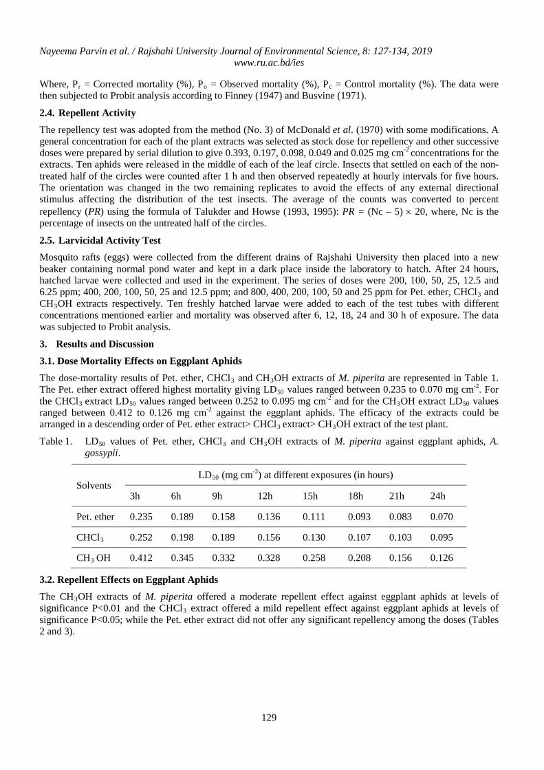
Nayeema Parvin et al. / Rajshahi University Journal of Environmental Science, 8: 127-134, 2019 www.ru.ac.bd/ies
129
Where, Pr = Corrected mortality (%), Po = Observed mortality (%), Pc = Control mortality (%). The data were then subjected to Probit analysis according to Finney (1947) and Busvine (1971).
2.4. Repellent Activity
The repellency test was adopted from the method (No. 3) of McDonald et al. (1970) with some modifications. A general concentration for each of the plant extracts was selected as stock dose for repellency and other successive doses were prepared by serial dilution to give 0.393, 0.197, 0.098, 0.049 and 0.025 mg cm-2 concentrations for the extracts. Ten aphids were released in the middle of each of the leaf circle. Insects that settled on each of the non-treated half of the circles were counted after 1 h and then observed repeatedly at hourly intervals for five hours. The orientation was changed in the two remaining replicates to avoid the effects of any external directional stimulus affecting the distribution of the test insects. The average of the counts was converted to percent repellency (PR) using the formula of Talukder and Howse (1993, 1995): PR = (Nc – 5) × 20, where, Nc is the percentage of insects on the untreated half of the circles.
2.5. Larvicidal Activity Test
Mosquito rafts (eggs) were collected from the different drains of Rajshahi University then placed into a new beaker containing normal pond water and kept in a dark place inside the laboratory to hatch. After 24 hours, hatched larvae were collected and used in the experiment. The series of doses were 200, 100, 50, 25, 12.5 and 6.25 ppm; 400, 200, 100, 50, 25 and 12.5 ppm; and 800, 400, 200, 100, 50 and 25 ppm for Pet. ether, CHCl3 and CH3OH extracts respectively. Ten freshly hatched larvae were added to each of the test tubes with different concentrations mentioned earlier and mortality was observed after 6, 12, 18, 24 and 30 h of exposure. The data was subjected to Probit analysis.
3. Results and Discussion
3.1. Dose Mortality Effects on Eggplant Aphids
The dose-mortality results of Pet. ether, CHCl3 and CH3OH extracts of M. piperita are represented in Table 1. The Pet. ether extract offered highest mortality giving LD50 values ranged between 0.235 to 0.070 mg cm-2. For the CHCl3 extract LD50 values ranged between 0.252 to 0.095 mg cm-2 and for the CH3OH extract LD50 values ranged between 0.412 to 0.126 mg cm-2 against the eggplant aphids. The efficacy of the extracts could be arranged in a descending order of Pet. ether extract> CHCl3 extract> CH3OH extract of the test plant.
Table 1. LD50 values of Pet. ether, CHCl3 and CH3OH extracts of M. piperita against eggplant aphids, A. gossypii.
Solvents LD50 (mg cm-2) at different exposures (in hours)
3h 6h 9h 12h 15h 18h 21h 24h
Pet. ether 0.235 0.189 0.158 0.136 0.111 0.093 0.083 0.070
CHCl3 0.252 0.198 0.189 0.156 0.130 0.107 0.103 0.095
CH3 OH 0.412 0.345 0.332 0.328 0.258 0.208 0.156 0.126
3.2. Repellent Effects on Eggplant Aphids
The CH3OH extracts of M. piperita offered a moderate repellent effect against eggplant aphids at levels of significance P<0.01 and the CHCl3 extract offered a mild repellent effect against eggplant aphids at levels of significance P<0.05; while the Pet. ether extract did not offer any significant repellency among the doses (Tables 2 and 3).
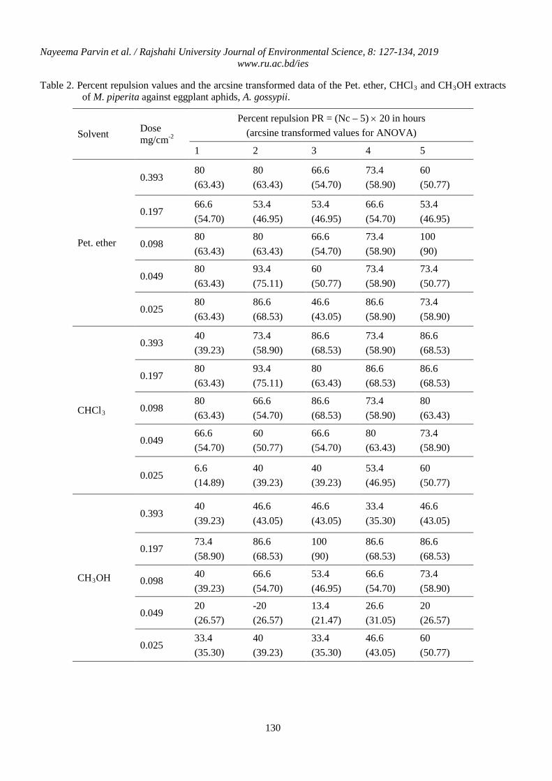
Nayeema Parvin et al. / Rajshahi University Journal of Environmental Science, 8: 127-134, 2019 www.ru.ac.bd/ies
130
Table 2. Percent repulsion values and the arcsine transformed data of the Pet. ether, CHCl3 and CH3OH extracts of M. piperita against eggplant aphids, A. gossypii.
Solvent Dose mg/cm-2
Percent repulsion PR = (Nc – 5) × 20 in hours (arcsine transformed values for ANOVA)
1 2 3 4 5
Pet. ether
0.393 80 (63.43)
80 (63.43)
66.6 (54.70)
73.4 (58.90)
60 (50.77)
0.197 66.6 (54.70)
53.4 (46.95)
53.4 (46.95)
66.6 (54.70)
53.4 (46.95)
0.098 80 (63.43)
80 (63.43)
66.6 (54.70)
73.4 (58.90)
100 (90)
0.049 80 (63.43)
93.4 (75.11)
60 (50.77)
73.4 (58.90)
73.4 (50.77)
0.025 80 (63.43)
86.6 (68.53)
46.6 (43.05)
86.6 (58.90)
73.4 (58.90)
CHCl3
0.393 40 (39.23)
73.4 (58.90)
86.6 (68.53)
73.4 (58.90)
86.6 (68.53)
0.197 80 (63.43)
93.4 (75.11)
80 (63.43)
86.6 (68.53)
86.6 (68.53)
0.098 80 (63.43)
66.6 (54.70)
86.6 (68.53)
73.4 (58.90)
80 (63.43)
0.049 66.6 (54.70)
60 (50.77)
66.6 (54.70)
80 (63.43)
73.4 (58.90)
0.025 6.6 (14.89)
40 (39.23)
40 (39.23)
53.4 (46.95)
60 (50.77)
CH3OH
0.393 40 (39.23)
46.6 (43.05)
46.6 (43.05)
33.4 (35.30)
46.6 (43.05)
0.197 73.4 (58.90)
86.6 (68.53)
100 (90)
86.6 (68.53)
86.6 (68.53)
0.098 40 (39.23)
66.6 (54.70)
53.4 (46.95)
66.6 (54.70)
73.4 (58.90)
0.049 20 (26.57)
-20 (26.57)
13.4 (21.47)
26.6 (31.05)
20 (26.57)
0.025 33.4 (35.30)
40 (39.23)
33.4 (35.30)
46.6 (43.05)
60 (50.77)
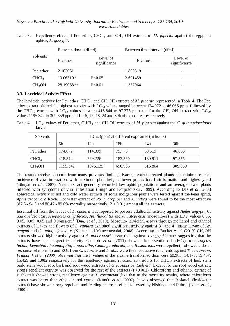
Nayeema Parvin et al. / Rajshahi University Journal of Environmental Science, 8: 127-134, 2019 www.ru.ac.bd/ies
131
Table 3. Repellency effect of Pet. ether, CHCl3 and CH3 OH extracts of M. piperita against the eggplant aphids, A. gossypii.
Solvents Between doses (df =4) Between time interval (df=4)
F-values Level of significance F-values Level of
significance
Pet. ether 2.183051 1.800319 - CHCl3 10.06319* P<0.05 2.691459 - CH3OH 28.19058** P<0.01 1.377064 -
3.3. Larvicidal Activity Effect
The larvicidal activity for Pet. ether, CHCl3 and CH3OH extracts of M. piperita represented in Table 4. The Pet. ether extract offered the highest activity with LC50 values ranged between 174.072 to 46.065 ppm, followed by the CHCl3 extract with LC50 values between 418.844 to 97.375 ppm and for the CH3 OH extract with LC50 values 1195.342 to 309.859 ppm all for 6, 12, 18, 24 and 30h of exposures respectively.
Table 4. LC50 values of Pet. ether, CHCl3 and CH3OH extracts of M. piperita against the C. quinquefasciatus larvae.
Solvents LC50 (ppm) at different exposures (in hours)
6h 12h 18h 24h 30h
Pet. ether 174.072 114.399 79.776 60.519 46.065
CHCl3 418.844 229.226 183.390 130.911 97.375
CH3OH 1195.342 1075.135 696.966 516.804 309.859
The results receive supports from many previous findings. Karanja extract treated plants had minimal rate of incidence of viral infestation, with maximum plant height, flower production, fruit formation and highest yield (Bhuyan et al., 2007). Neem extract generally recorded low aphid populations and an average fewer plants infected with symptoms of viral infestation (Singh and Korpraditskul, 1999). According to Das et al., 2008 aphidicidal activity of hot and cold water extracts of some indigenous plants were tested against the bean aphid, Aphis craccivora Koch. Hot water extract of Po. hydropiper and A. indica were found to be the most effective (87.6 - 94.5 and 80.47 - 89.6% mortality respectively, P < 0.01) among all the extracts.
Essential oil from the leaves of L. camara was reported to possess adulticidal activity against Aedes aegypti, C. quinquefasciatus, Anopheles culicifacies, An. fluvialitis and An. stephensi (mosquitoes) with LD50 values 0.06, 0.05, 0.05, 0.05 and 0.06mg/cm2 (Dua, et al., 2010). Mosquito larvicidal assays through methanol and ethanol extracts of leaves and flowers of L. camara exhibited significant activity against 3rd and 4th instar larvae of Ae. aegypti and C. quinquefasciatus (Kumar and Maneemegalai, 2008). According to Bucker et al. (2013) CH3OH extracts showed higher activity against A. nuneztovari larvae than against A. aegypti larvae, suggesting that the extracts have species-specific activity. Gallardo et al. (2011) showed that essential oils (EOs) from Tagetes lucida, Lepechinia betonicifolia, Lippia alba, Cananga odorata, and Rosmarinus were repellent, followed a dose-response relationship and EOs from C. odorata and L. alba were the most active repellents against T. castaneum. Pramanik et al. (2009) observed that the F values of the arcsine transformed data were 60.983, 14.177, 19.437, 15.429 and 1.082 respectively for the repellency against T. castaneum adults for CHCI3 extracts of leaf, stem bark, stem wood, root bark and root wood extracts of Glycosmis pentaphylla. Except for the root wood extract, strong repellent activity was observed for the rest of the extracts (P<0.001). Chloroform and ethanol extract of Bishkatali showed strong repellency against T. castaneum (like that of the mortality results) where chloroform extract was better than ethyl alcohol extract (Kundu et al., 2007). It was observed that Biskatali (leaf/water extract) have shown strong repellent and feeding deterrent effect followed by Nishinda and Pithraj (Islam et al., 2000).
Nayeema Parvin et al. / Rajshahi University Journal of Environmental Science, 8: 127-134, 2019 www.ru.ac.bd/ies
132
Thus, a comprehensive phytochemical analyses of the M. piperita for its insecticidal, repellent and larvicidal components, as well as the physiological studies of the active ingredients is very much to be solicited for their effective use in the future vector control and pharmaceutical endeavors.
Acknowledgements
The authors are grateful to Bangladesh Agricultural Development Corporation (BADC) of the Bangladesh Government for granting three years deputation for research in the IES. They would like to woe their best regards to the honorable Director, Institute of Environmental Science (IES), University of Rajshahi for providing laboratory facilities.
References
Abbott WS. 1925. A method of computing the effectiveness of an insecticide. J. Econ. Entomol., 18: 265-267.
Ahmed ZU, Hassan MA and Kabir SMH (eds). 2009. Encyclopedia of flora and fauna of Bangladesh, Angiosperms, Dicotyledons. Asiatic Society of Bangladesh.7: 257p.
Alexa E, Danciu C, Radulov I, Obistioiu D, Sumalan RM, Morar A and Dehelean CA. 2018. Phytochemical screening and biological activity of Mentha piperita L. and Lavandulaangustifolia Mill. extracts. Analytical Cellular Pathol., 2018: Article ID 2678924, https://doi.org/10.1155/2018/2678924.
Al-Rajab AJ, Sharma M, Moses MM, Reddy GR and AlbrattyM. 2018. Chemical constituents, in vitro antibacterial and antifungal activity of Mentha piperita L. (peppermint) essential oil. J. King Saud Univ.– Sci. 31(4):528-533.
Astier S, Albouy J, Maury Y and Lecoq H. 2001. Principes de virologievégétale: génome, pouvoirpathogène, écologie des virus. Paris, FRA: INRA Editions, 444p. https://prodinra.inra.fr/record/55828
Bhuyan SB, Alam MM and Ali MS. 2007. Effect of plant extracts on Okra mosaic virus incidence and yield related parameters of Okra. Asian J. Agri. Res.,1: 112-118.
Brahmi F, Khodir M, Mohamed C and Pierre D. 2017. Chemical Composition and Biological Activities of Mentha Species, Aromatic and Medicinal Plants, In: Back to Nature, Hany A. El-Shemy, Intech. Open. DOI: 10.5772/67291.
Bucker A, Bucker NC, Souza AQ, Gama A, Rodrigues-Filho E, Costa F, Nunez CV, Castro e Silva A and Tadei WP. 2013. Larvicidal effects of endophytic and basidiomycete fungus extracts on Aedes and Anopheles larvae (Diptera, Culicidae). Rev. Soc. Bras. Med. Trop., 46: 411-9.
Busvine JR. 1971. A critical review of the techniques for testing insecticides. Commonwealth Agricultural Bureaux, London. 345p.
Carson R.1962. Silent Spring. Boston: Houghton Mifflin. Riverside Press, 336 pp.
Das BC, Sarker PK and Rahman MM. 2008. Aphidicidal activity of some indegenous plant extracts against bean aphid Aphis craccivora Koch. (Homoptera:Aphididae). J. Pest Sci., 81: 153-159.
Dua VK, Pandey AC and Dash AP. 2010. Adulticidal activity of essential oil of Lantana camara leaves against mosquitoes. Indian J. Med. Res.,131: 434-439.
Finney DJ. 1947. Probit analysis: a statistical treatment of the sigmoid response curve. Cambridge University Press, London. 333p.
Gallardo KC, Verbel JO and Stashenko EE. 2011. Repellent activity of essential oils and some of their individual constituents against Tribolium castaneum. Environmental and Computational Chemistry Group, Faculty of Pharmaceutical Sciences, University of Cartagena, Cartagena, Colombia. J. Agric. Food Chem., 59(5): 1690-1696.
Giri B, Amutha C, Siddhan N, Murali KS. 2007. Antibacterial activity of Mentha piperita L. (peppermint) from leaf extracts - A medicinal plant. Acta Agric. Slovenica, 89-1, (1):73-79.
Nayeema Parvin et al. / Rajshahi University Journal of Environmental Science, 8: 127-134, 2019 www.ru.ac.bd/ies
133
Gökalpİşcan, Neşe Kı̇rı̇mer, Mı̇ne Kürkcüoǧlu, Hüsnü Can Başerand Fatı̇h Demı̇rcı̇ 2002. Antimicrobial screening of Mentha piperita essential oils. J. Agric. Food Chem., 50(14): 3943–3946. https://doi.org/10.1021/jf011476k
Haydari M, Maresca V, Rigano D, Taleei A, Shahnejat-Bushehri AA, Hadian J,Sorbo S, Guida M, Manna C, Piscopo M, Notariale R, De Ruberto F, Fusaro L and Basile A. 2019. Salicylic Acid and Melatonin Alleviate the Effects of Heat Stress on Essential Oil Composition and Antioxidant Enzyme Activity in Mentha piperita and Mentha arvensis L. Antioxidants, 8(11): 547; https://doi.org/10.3390/antiox8110547
Islam ASMN. 2010. Pesticide use in Bangladesh tripled in 10 years. BRRI. Agricultural Economics Division. (http://news.agropages.com)
Islam ATMF, Akther S, Islam S and Huque R. 2000. Repellent and feeding deferrent effects of some indigenous plants against red flour beetle, Triboliumcasteneum (Herbst) (Coleoptera:Tenebrionldae). Pak. J. Agri. Sci., 37(1-2): 11-15.
Jain SK. 1991. Dictionary of Indian folk medicine and Ethnobotany. New Delhi: Deep Publishing. 92p.
Jaouni SA, Saleh AM, WadaanMAM, Hozzein WN, Selim S and Elgawad HA. 2018. Elevated CO2 induces a global metabolic change in basil (Ocimum basilicum L.) and peppermint (Mentha piperita L.) and improves their biological activity.J. Plant Physiol., 224–225: 121-131.
Kumar MS and Maneemegalai S. 2008. Evaluation of larvicidal effect of Lantana Camara Linn. against mosquito species Aedesaegypti and Culexquinque fasciatus. Advances Biol. Res., 2(3-4): 39-43.
Kundu BR, Ara R, Begum MM and Sarker ZI. 2007. Effect of Bishkatali, Polygonum hydropiper L. plant extracts against the red flour beetle, Tribolium castaneum (Herbst). Univ. J. Zool. Rajshahi Univ., 26:93-97.
Manandhar NP. 2002. Plants and People of Nepal. Timber Press, 230p.
McDonald LL, Guy RH and Speirs RD. 1970. Preliminary evaluation of new candidate materials as toxicants, repellents and attractants against stored-product insects. Marketing Research Report No. 882. Agricultural Research Service, US Department of Agriculture, Washington, DC.
Michigan Mosquito Control Organization. 2013. Mosquitoes of Michigan-Their biology and control. Michigan Mosquito Control Manual, Michigan, USA.
Pesticide Action Network, August 2010. Environmental effects of pesticides. An impression of recent scientific literature.
Pramanik MS, Akter MY, Ekram AE, Islam H, Khan AR and Islam N. 2009. Screening of Glycosmis pentaphylla for cytotoxic and repellent potentials against Artemia salina nauplii and Tribolium castaneum (Herbst) adults. J. Life Earth Sci., 3(4), 33-36.
Singh H and Korpraditskul V. 1999. Evaluation of some plant extracts against aphids, key vectors of chilly-virus complex Azadirachtaindica A Juss., (Eds. R.P. Singh and R.C. Saxena). pp139-146.
Singh R, Shushni MAM and Belkheir A. 2015. Antibacterial and antioxidental activities of Mentha piperita L. Arabian J. Chem., 8(3): 322-328.
Talukder FA, Howse PE. 1993. Deterrent and insecticidal effects of extracts of Pithraj, Aphanamixispolystachya (Meliaceae), against Tribolium castaneum in storage. J. Chemi. Ecol., 19(11):2463-2471.
Talukder FA, Howse PE. 1995. Evaluation of Aphanamixis polystachya as a source of repellents, antifeedants, toxicants and protectants in storage against Tribolium castaneum (Herbst), J. Stored Prod. Res., 31(1):55-61.

Nayeema Parvin et al. / Rajshahi University Journal of Environmental Science, 8: 127-134, 2019 www.ru.ac.bd/ies
134
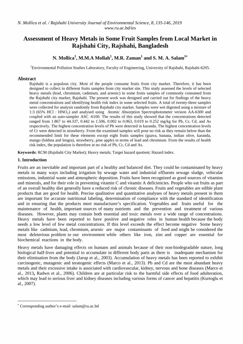
N. Mollica et al. / Rajshahi University Journal of Environmental Science, 8, 135-146, 2019 www.ru.ac.bd/ies
Assessment of Heavy Metals in Some Fruit Samples from Local Market in Rajshahi City, Rajshahi, Bangladesh
N. Mollica1, M.M.A Mollah1, M.R. Zaman1 and S. M. A. Salam1∗
1Environmental Pollution Studies Laboratory, Faculty of Engineering, University of Rajshahi, Rajshahi-6205.
Abstract
Rajshahi is a populous city. Most of the people consume fruits from city market. Therefore, it has been designed to collect in different fruits samples from city market site. This study assessed the levels of selected heavy metals (lead, chromium, cadmium, and arsenic) in some fruits samples of commonly consumed from the Rajshahi city market, Rajshahi. The present work was designed and carried out for findings of the heavy metal concentrations and identifying health risk index in some selected fruits. A total of twenty-three samples were collected for analysis randomly from Rajshahi city market. Samples were wet digested using a mixture of 1:3 (65% HCl : HNO3) and analysed using Atomic Absorption Spectrophotometer version AA-6300 and coupled with an auto-sampler ASC -6100. The results of this study showed that the concentrations detected ranged from 1.867 to 44.337, 0.442 to 1.506, 0.002 to 0.063, 0.019 to 0.252 mg/kg for Pb, Cr, Cd, and As respectively. The highest concentration levels of Pb were detected in karanda. The highest concentration levels of Cr were detected in strawberry. From the examined samples will pose no risk as they remain below than the recommended limit for these elements except eight fruits samples (guava, banana, indian olive, karanda, mango (lokhna and lengra), strawberry, pine apple) in terms of lead and chromium. From the results of health risk index, the population is therefore at no risk of Pb, Cr, Cd and As.
Keywords: RCM (Rajshahi City Market); Heavy metals; Target hazard quotient; Hazard index.
1. Introduction
Fruits are an inevitable and important part of a healthy and balanced diet. They could be contaminated by heavy metals in many ways including irrigation by sewage water and industrial effluents sewage sludge, vehicular emissions, industrial waste and atmospheric deposition. Fruits have been recognized as good sources of vitamins and minerals, and for their role in preventing vitamin C and vitamin A deficiencies. People who eat fruits as part of an overall healthy diet generally have a reduced risk of chronic diseases. Fruits and vegetables are edible plant products that are good for health. Precise qualitative and quantitative analyses of heavy metals present in them are important for accurate nutritional labeling, determination of compliance with the standard of identification and in ensuring that the products meet manufacturer’s specification. Vegetables and fruits useful for the maintenance of health, important sources of many nutrients and the prevention and treatment of various diseases. However, plants may contain both essential and toxic metals over a wide range of concentrations. Heavy metals have been reported to have positive and negative roles in human health because the body needs a low level of few metal concentrations. If this level exceeds the effect become negative Some heavy metals like cadmium, lead, chromium, arsenic are major contaminants of food and might be considered the most deleterious problem to our environment while others like iron, zinc and copper are essential for biochemical reactions in the body.
Heavy metals have damaging effects on humans and animals because of their non-biodegradable nature, long biological half-lives and potential to accumulate in different body parts as there is inadequate mechanism for their elimination from the body (Jarup et al., 2003). Accumulation of heavy metals has been reported to exhibit carcinogenic, mutagenic and teratogenic effects (Marco et al., 2013). Pb and Cd are the most abundant heavy metals and their excessive intake is associated with cardiovascular, kidney, nervous and bone diseases (Marco et al., 2013, Radwn et al., 2006). Children are at particular risk to the harmful side effects of food adulteration, which may lead to serious liver and kidney diseases including various forms of cancer and hepatitis (Kurtoglu et al., 2007).
∗ Corresponding author’s e-mail: [email protected]
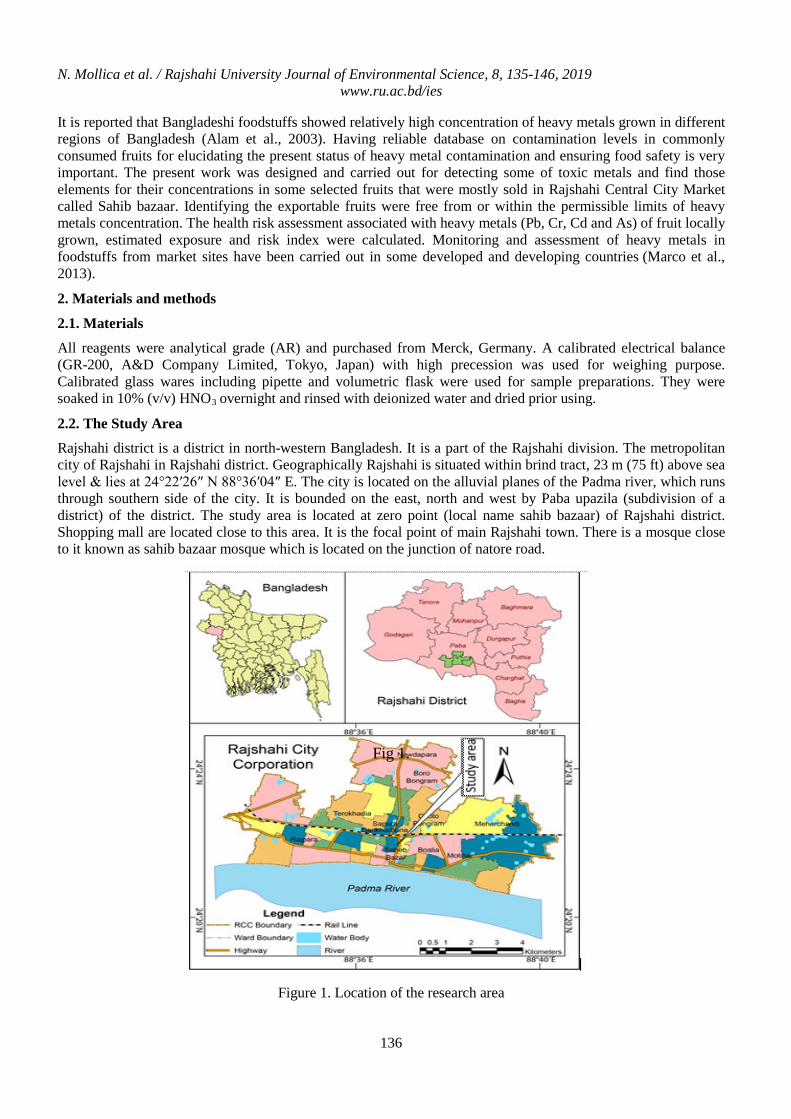
N. Mollica et al. / Rajshahi University Journal of Environmental Science, 8, 135-146, 2019 www.ru.ac.bd/ies
136
It is reported that Bangladeshi foodstuffs showed relatively high concentration of heavy metals grown in different regions of Bangladesh (Alam et al., 2003). Having reliable database on contamination levels in commonly consumed fruits for elucidating the present status of heavy metal contamination and ensuring food safety is very important. The present work was designed and carried out for detecting some of toxic metals and find those elements for their concentrations in some selected fruits that were mostly sold in Rajshahi Central City Market called Sahib bazaar. Identifying the exportable fruits were free from or within the permissible limits of heavy metals concentration. The health risk assessment associated with heavy metals (Pb, Cr, Cd and As) of fruit locally grown, estimated exposure and risk index were calculated. Monitoring and assessment of heavy metals in foodstuffs from market sites have been carried out in some developed and developing countries (Marco et al., 2013).
2. Materials and methods
2.1. Materials All reagents were analytical grade (AR) and purchased from Merck, Germany. A calibrated electrical balance (GR-200, A&D Company Limited, Tokyo, Japan) with high precession was used for weighing purpose. Calibrated glass wares including pipette and volumetric flask were used for sample preparations. They were soaked in 10% (v/v) HNO3 overnight and rinsed with deionized water and dried prior using.
2.2. The Study Area
Rajshahi district is a district in north-western Bangladesh. It is a part of the Rajshahi division. The metropolitan city of Rajshahi in Rajshahi district. Geographically Rajshahi is situated within brind tract, 23 m (75 ft) above sea level & lies at 24°22′26″ N 88°36′04″ E. The city is located on the alluvial planes of the Padma river, which runs through southern side of the city. It is bounded on the east, north and west by Paba upazila (subdivision of a district) of the district. The study area is located at zero point (local name sahib bazaar) of Rajshahi district. Shopping mall are located close to this area. It is the focal point of main Rajshahi town. There is a mosque close to it known as sahib bazaar mosque which is located on the junction of natore road.
Fig 1.
Figure 1. Location of the research area
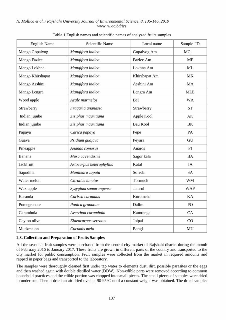
N. Mollica et al. / Rajshahi University Journal of Environmental Science, 8, 135-146, 2019 www.ru.ac.bd/ies
137
Table 1 English names and scientific names of analyzed fruits samples
English Name Scientific Name Local name Sample ID
Mango Gopalvog Mangifera indica Gopalvog Am MG
Mango Fazlee Mangifera indica Fazlee Am MF
Mango Lokhna Mangifera indica Lokhna Am ML
Mango Khirshapat Mangifera indica Khirshapat Am MK
Mango Asshini Mangifera indica Asshini Am MA
Mango Lengra Mangifera indica Lengra Am MLE
Wood apple Aegle marmelos Bel WA
Strawberry Fragaria ananassa Strawberry ST
Indian jujube Ziziphus mauritiana Apple Kool AK
Indian jujube Ziziphus mauritiana Bau Kool BK
Papaya Carica papaya Pepe PA
Guava Psidium guajava Peyara GU
Pineapple Ananas comosus Anaros PI
Banana Musa cavendishii Sagor kala BA
Jackfruit Artocarpus heterophyllus Katal JA
Sapodilla Manilkara zapota Sofeda SA
Water melon Citrullus lanatus Tormuch WM
Wax apple Syzygium samarangense Jamrul WAP
Karanda Carissa carandas Koromcha KA
Pomegranate Punica granatum Dalim PO
Carambola Averrhoa carambola Kamranga CA
Ceylon olive Elaeocarpus serratus Jolpai CO
Muskmelon Cucumis melo Bangi MU
2.3. Collection and Preparation of Fruits Samples
All the seasonal fruit samples were purchased from the central city market of Rajshahi district during the month of February 2016 to January 2017. These fruits are grown in different parts of the country and transported to the city market for public consumption. Fruit samples were collected from the market in required amounts and rapped in paper bags and transported to the laboratory.
The samples were thoroughly cleaned first under tap water to elements dust, dirt, possible parasites or the eggs and then washed again with double distilled water (DDW). Non-edible parts were removed according to common household practices and the edible portion was chopped into small pieces. The small pieces of samples were dried in under sun. Then it dried an air dried oven at 90-95°C until a constant weight was obtained. The dried samples
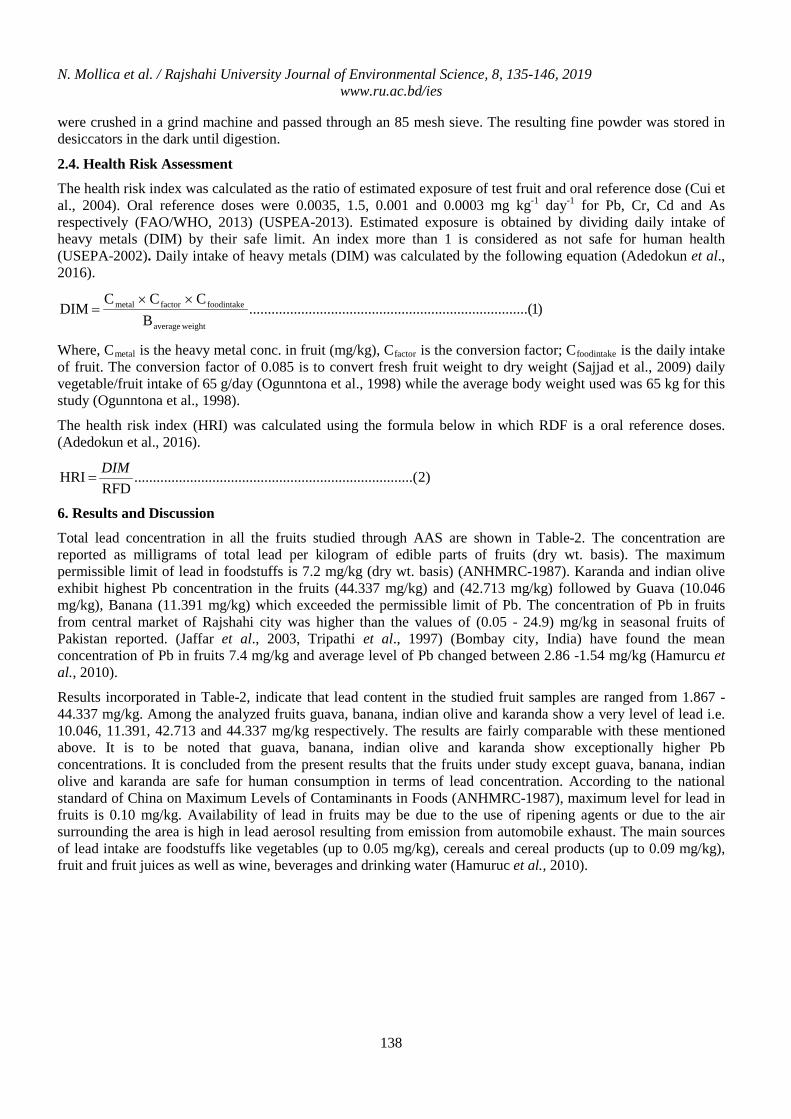
N. Mollica et al. / Rajshahi University Journal of Environmental Science, 8, 135-146, 2019 www.ru.ac.bd/ies
138
were crushed in a grind machine and passed through an 85 mesh sieve. The resulting fine powder was stored in desiccators in the dark until digestion.
2.4. Health Risk Assessment
The health risk index was calculated as the ratio of estimated exposure of test fruit and oral reference dose (Cui et al., 2004). Oral reference doses were 0.0035, 1.5, 0.001 and 0.0003 mg kg-1 day-1 for Pb, Cr, Cd and As respectively (FAO/WHO, 2013) (USPEA-2013). Estimated exposure is obtained by dividing daily intake of heavy metals (DIM) by their safe limit. An index more than 1 is considered as not safe for human health (USEPA-2002). Daily intake of heavy metals (DIM) was calculated by the following equation (Adedokun et al., 2016).
)1.....(......................................................................B
CCC DIM
weightaverage
foodintakefactormetal ××=
Where, Cmetal is the heavy metal conc. in fruit (mg/kg), Cfactor is the conversion factor; Cfoodintake is the daily intake of fruit. The conversion factor of 0.085 is to convert fresh fruit weight to dry weight (Sajjad et al., 2009) daily vegetable/fruit intake of 65 g/day (Ogunntona et al., 1998) while the average body weight used was 65 kg for this study (Ogunntona et al., 1998).
The health risk index (HRI) was calculated using the formula below in which RDF is a oral reference doses. (Adedokun et al., 2016).
)2.....(......................................................................RFD
HRI DIM=
6. Results and Discussion
Total lead concentration in all the fruits studied through AAS are shown in Table-2. The concentration are reported as milligrams of total lead per kilogram of edible parts of fruits (dry wt. basis). The maximum permissible limit of lead in foodstuffs is 7.2 mg/kg (dry wt. basis) (ANHMRC-1987). Karanda and indian olive exhibit highest Pb concentration in the fruits (44.337 mg/kg) and (42.713 mg/kg) followed by Guava (10.046 mg/kg), Banana (11.391 mg/kg) which exceeded the permissible limit of Pb. The concentration of Pb in fruits from central market of Rajshahi city was higher than the values of (0.05 - 24.9) mg/kg in seasonal fruits of Pakistan reported. (Jaffar et al., 2003, Tripathi et al., 1997) (Bombay city, India) have found the mean concentration of Pb in fruits 7.4 mg/kg and average level of Pb changed between 2.86 -1.54 mg/kg (Hamurcu et al., 2010).
Results incorporated in Table-2, indicate that lead content in the studied fruit samples are ranged from 1.867 - 44.337 mg/kg. Among the analyzed fruits guava, banana, indian olive and karanda show a very level of lead i.e. 10.046, 11.391, 42.713 and 44.337 mg/kg respectively. The results are fairly comparable with these mentioned above. It is to be noted that guava, banana, indian olive and karanda show exceptionally higher Pb concentrations. It is concluded from the present results that the fruits under study except guava, banana, indian olive and karanda are safe for human consumption in terms of lead concentration. According to the national standard of China on Maximum Levels of Contaminants in Foods (ANHMRC-1987), maximum level for lead in fruits is 0.10 mg/kg. Availability of lead in fruits may be due to the use of ripening agents or due to the air surrounding the area is high in lead aerosol resulting from emission from automobile exhaust. The main sources of lead intake are foodstuffs like vegetables (up to 0.05 mg/kg), cereals and cereal products (up to 0.09 mg/kg), fruit and fruit juices as well as wine, beverages and drinking water (Hamuruc et al., 2010).
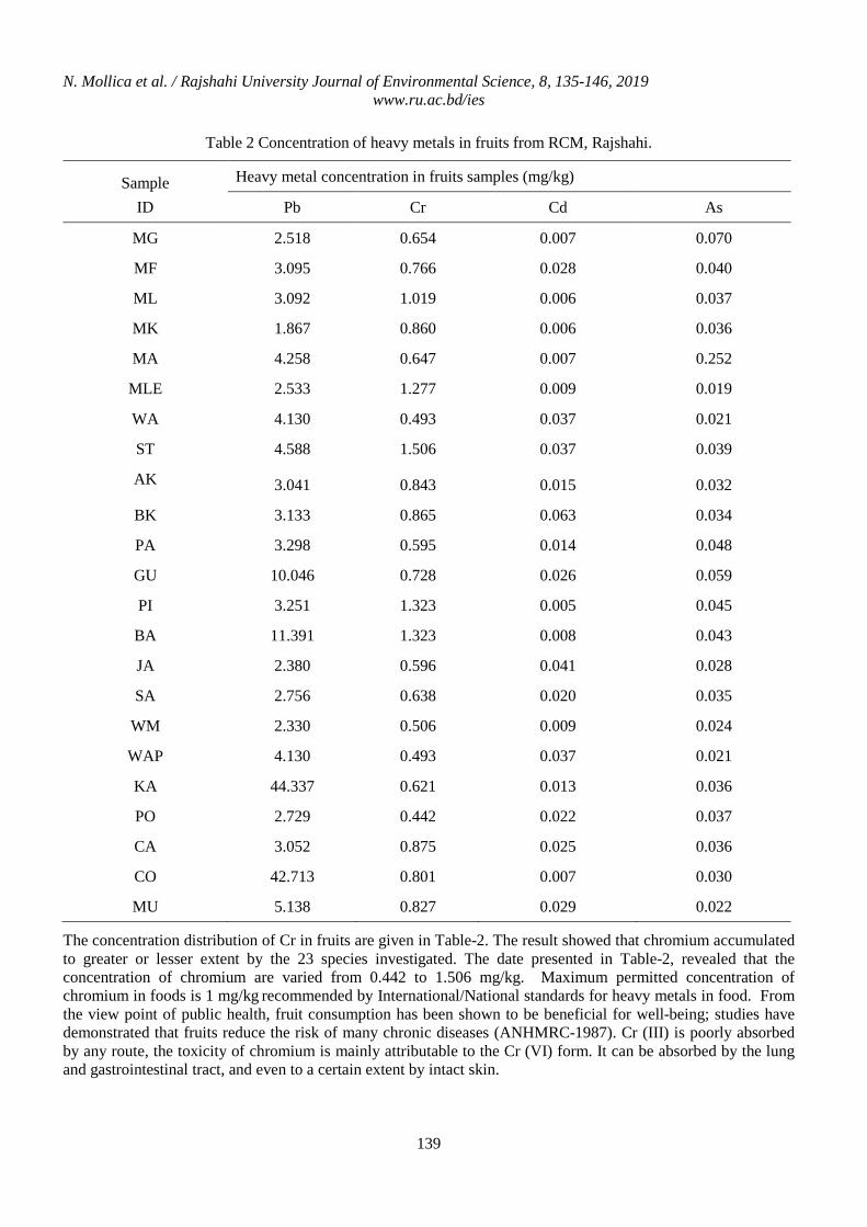
N. Mollica et al. / Rajshahi University Journal of Environmental Science, 8, 135-146, 2019 www.ru.ac.bd/ies
139
Table 2 Concentration of heavy metals in fruits from RCM, Rajshahi.
Sample ID
Heavy metal concentration in fruits samples (mg/kg)
Pb Cr Cd As
MG 2.518 0.654 0.007 0.070
MF 3.095 0.766 0.028 0.040
ML 3.092 1.019 0.006 0.037
MK 1.867 0.860 0.006 0.036
MA 4.258 0.647 0.007 0.252
MLE 2.533 1.277 0.009 0.019
WA 4.130 0.493 0.037 0.021
ST 4.588 1.506 0.037 0.039
AK 3.041 0.843 0.015 0.032
BK 3.133 0.865 0.063 0.034
PA 3.298 0.595 0.014 0.048
GU 10.046 0.728 0.026 0.059
PI 3.251 1.323 0.005 0.045
BA 11.391 1.323 0.008 0.043
JA 2.380 0.596 0.041 0.028
SA 2.756 0.638 0.020 0.035
WM 2.330 0.506 0.009 0.024
WAP 4.130 0.493 0.037 0.021
KA 44.337 0.621 0.013 0.036
PO 2.729 0.442 0.022 0.037
CA 3.052 0.875 0.025 0.036
CO 42.713 0.801 0.007 0.030
MU 5.138 0.827 0.029 0.022
The concentration distribution of Cr in fruits are given in Table-2. The result showed that chromium accumulated to greater or lesser extent by the 23 species investigated. The date presented in Table-2, revealed that the concentration of chromium are varied from 0.442 to 1.506 mg/kg. Maximum permitted concentration of chromium in foods is 1 mg/kg recommended by International/National standards for heavy metals in food. From the view point of public health, fruit consumption has been shown to be beneficial for well-being; studies have demonstrated that fruits reduce the risk of many chronic diseases (ANHMRC-1987). Cr (III) is poorly absorbed by any route, the toxicity of chromium is mainly attributable to the Cr (VI) form. It can be absorbed by the lung and gastrointestinal tract, and even to a certain extent by intact skin.
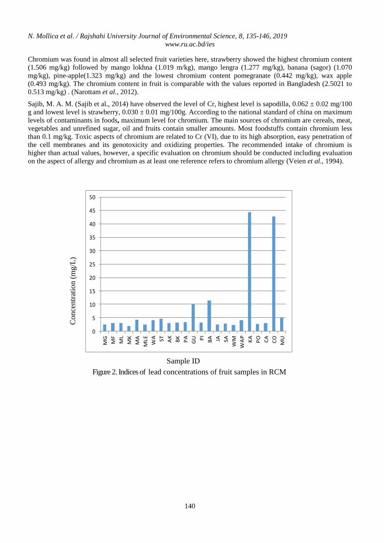
N. Mollica et al. / Rajshahi University Journal of Environmental Science, 8, 135-146, 2019 www.ru.ac.bd/ies
140
Chromium was found in almost all selected fruit varieties here, strawberry showed the highest chromium content (1.506 mg/kg) followed by mango lokhna (1.019 m/kg), mango lengra (1.277 mg/kg), banana (sagor) (1.070 mg/kg), pine-apple(1.323 mg/kg) and the lowest chromium content pomegranate (0.442 mg/kg), wax apple (0.493 mg/kg). The chromium content in fruit is comparable with the values reported in Bangladesh (2.5021 to 0.513 mg/kg) . (Narottam et al., 2012).
Sajib, M. A. M. (Sajib et al., 2014) have observed the level of Cr, highest level is sapodilla, 0.062 ± 0.02 mg/100 g and lowest level is strawberry, 0.030 ± 0.01 mg/100g. According to the national standard of china on maximum levels of contaminants in foods, maximum level for chromium. The main sources of chromium are cereals, meat, vegetables and unrefined sugar, oil and fruits contain smaller amounts. Most foodstuffs contain chromium less than 0.1 mg/kg. Toxic aspects of chromium are related to Cr (VI), due to its high absorption, easy penetration of the cell membranes and its genotoxicity and oxidizing properties. The recommended intake of chromium is higher than actual values, however, a specific evaluation on chromium should be conducted including evaluation on the aspect of allergy and chromium as at least one reference refers to chromium allergy (Veien et al., 1994).
0
5
10
15
20
25
30
35
40
45
50
MG
MF
ML
MK
MA
MLE WA ST AK
BK PA GU PI BA JA SA
WM
WA
PKA PO CA CO MU
Figure 2. Indices of lead concentrations of fruit samples in RCM
Con
cent
ratio
n (m
g/L)
Sample ID
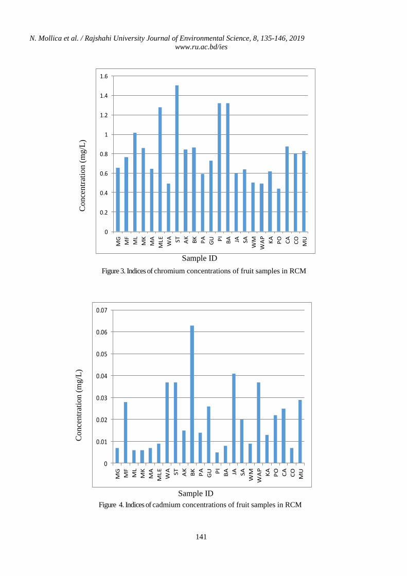
N. Mollica et al. / Rajshahi University Journal of Environmental Science, 8, 135-146, 2019 www.ru.ac.bd/ies
141
0
0.2
0.4
0.6
0.8
1
1.2
1.4
1.6
MG
MF
ML
MK
MA
MLE WA ST AK BK PA GU PI BA JA SA
WM
WA
PKA PO CA CO MU
Figure 3. Indices of chromium concentrations of fruit samples in RCM
Con
cent
ratio
n (m
g/L)
Sample ID
0
0.01
0.02
0.03
0.04
0.05
0.06
0.07
MG
MF
ML
MK
MA
MLE
WA ST AK
BK PA GU PI BA JA SA
WM
WA
PKA PO CA CO MU
Figure 4. Indices of cadmium concentrations of fruit samples in RCM
Con
cent
ratio
n (m
g/L)
Sample ID
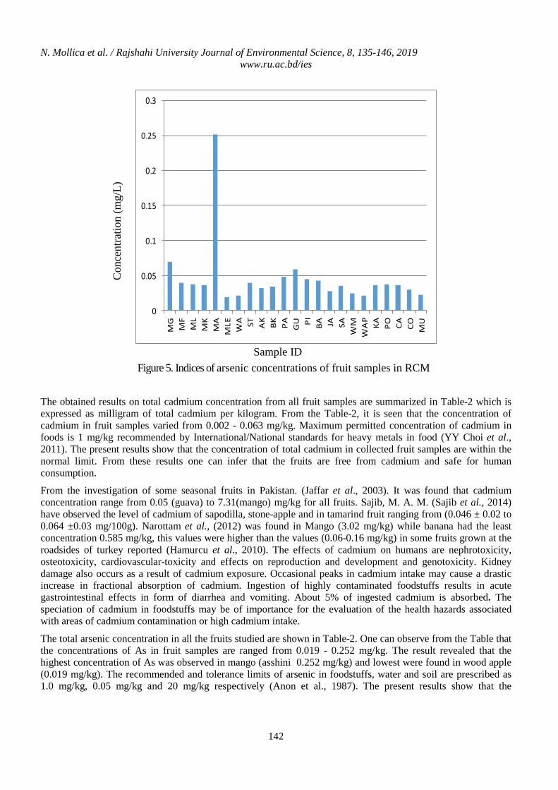
N. Mollica et al. / Rajshahi University Journal of Environmental Science, 8, 135-146, 2019 www.ru.ac.bd/ies
142
The obtained results on total cadmium concentration from all fruit samples are summarized in Table-2 which is expressed as milligram of total cadmium per kilogram. From the Table-2, it is seen that the concentration of cadmium in fruit samples varied from 0.002 - 0.063 mg/kg. Maximum permitted concentration of cadmium in foods is 1 mg/kg recommended by International/National standards for heavy metals in food (YY Choi et al., 2011). The present results show that the concentration of total cadmium in collected fruit samples are within the normal limit. From these results one can infer that the fruits are free from cadmium and safe for human consumption.
From the investigation of some seasonal fruits in Pakistan. (Jaffar et al., 2003). It was found that cadmium concentration range from 0.05 (guava) to 7.31(mango) mg/kg for all fruits. Sajib, M. A. M. (Sajib et al., 2014) have observed the level of cadmium of sapodilla, stone-apple and in tamarind fruit ranging from (0.046 ± 0.02 to 0.064 ±0.03 mg/100g). Narottam et al., (2012) was found in Mango (3.02 mg/kg) while banana had the least concentration 0.585 mg/kg, this values were higher than the values (0.06-0.16 mg/kg) in some fruits grown at the roadsides of turkey reported (Hamurcu et al., 2010). The effects of cadmium on humans are nephrotoxicity, osteotoxicity, cardiovascular-toxicity and effects on reproduction and development and genotoxicity. Kidney damage also occurs as a result of cadmium exposure. Occasional peaks in cadmium intake may cause a drastic increase in fractional absorption of cadmium. Ingestion of highly contaminated foodstuffs results in acute gastrointestinal effects in form of diarrhea and vomiting. About 5% of ingested cadmium is absorbed. The speciation of cadmium in foodstuffs may be of importance for the evaluation of the health hazards associated with areas of cadmium contamination or high cadmium intake.
The total arsenic concentration in all the fruits studied are shown in Table-2. One can observe from the Table that the concentrations of As in fruit samples are ranged from 0.019 - 0.252 mg/kg. The result revealed that the highest concentration of As was observed in mango (asshini 0.252 mg/kg) and lowest were found in wood apple (0.019 mg/kg). The recommended and tolerance limits of arsenic in foodstuffs, water and soil are prescribed as 1.0 mg/kg, 0.05 mg/kg and 20 mg/kg respectively (Anon et al., 1987). The present results show that the
0
0.05
0.1
0.15
0.2
0.25
0.3
MG
MF
ML
MK
MA
MLE
WA ST AK
BK PA GU PI BA JA SA
WM
WA
PKA PO CA CO MU
Figure 5. Indices of arsenic concentrations of fruit samples in RCM
Con
cent
ratio
n (m
g/L)
Sample ID
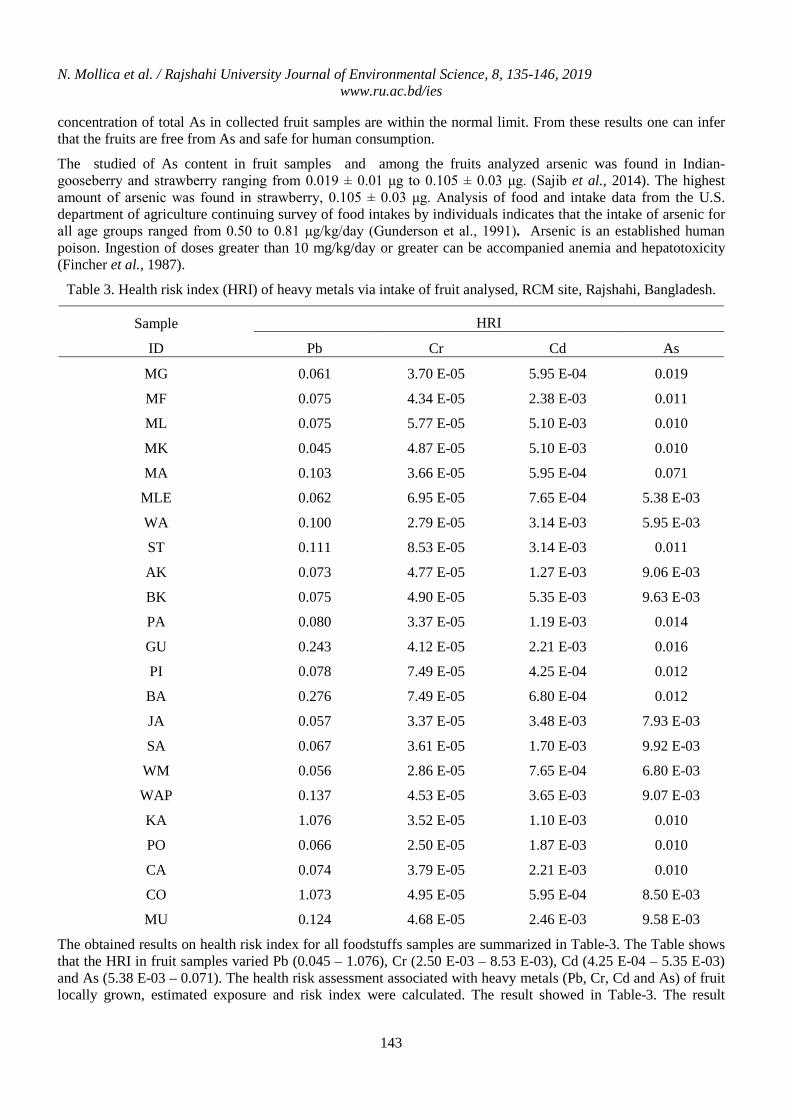
N. Mollica et al. / Rajshahi University Journal of Environmental Science, 8, 135-146, 2019 www.ru.ac.bd/ies
143
concentration of total As in collected fruit samples are within the normal limit. From these results one can infer that the fruits are free from As and safe for human consumption.
The studied of As content in fruit samples and among the fruits analyzed arsenic was found in Indian- gooseberry and strawberry ranging from 0.019 ± 0.01 μg to 0.105 ± 0.03 μg. (Sajib et al., 2014). The highest amount of arsenic was found in strawberry, 0.105 ± 0.03 μg. Analysis of food and intake data from the U.S. department of agriculture continuing survey of food intakes by individuals indicates that the intake of arsenic for all age groups ranged from 0.50 to 0.81 μg/kg/day (Gunderson et al., 1991). Arsenic is an established human poison. Ingestion of doses greater than 10 mg/kg/day or greater can be accompanied anemia and hepatotoxicity (Fincher et al., 1987).
Table 3. Health risk index (HRI) of heavy metals via intake of fruit analysed, RCM site, Rajshahi, Bangladesh.
Sample ID
HRI Pb Cr Cd As
MG 0.061 3.70 E-05 5.95 E-04 0.019 MF 0.075 4.34 E-05 2.38 E-03 0.011 ML 0.075 5.77 E-05 5.10 E-03 0.010 MK 0.045 4.87 E-05 5.10 E-03 0.010 MA 0.103 3.66 E-05 5.95 E-04 0.071
MLE 0.062 6.95 E-05 7.65 E-04 5.38 E-03 WA 0.100 2.79 E-05 3.14 E-03 5.95 E-03 ST 0.111 8.53 E-05 3.14 E-03 0.011 AK 0.073 4.77 E-05 1.27 E-03 9.06 E-03 BK 0.075 4.90 E-05 5.35 E-03 9.63 E-03 PA 0.080 3.37 E-05 1.19 E-03 0.014 GU 0.243 4.12 E-05 2.21 E-03 0.016 PI 0.078 7.49 E-05 4.25 E-04 0.012 BA 0.276 7.49 E-05 6.80 E-04 0.012 JA 0.057 3.37 E-05 3.48 E-03 7.93 E-03 SA 0.067 3.61 E-05 1.70 E-03 9.92 E-03
WM 0.056 2.86 E-05 7.65 E-04 6.80 E-03 WAP 0.137 4.53 E-05 3.65 E-03 9.07 E-03 KA 1.076 3.52 E-05 1.10 E-03 0.010 PO 0.066 2.50 E-05 1.87 E-03 0.010 CA 0.074 3.79 E-05 2.21 E-03 0.010 CO 1.073 4.95 E-05 5.95 E-04 8.50 E-03 MU 0.124 4.68 E-05 2.46 E-03 9.58 E-03
The obtained results on health risk index for all foodstuffs samples are summarized in Table-3. The Table shows that the HRI in fruit samples varied Pb (0.045 – 1.076), Cr (2.50 E-03 – 8.53 E-03), Cd (4.25 E-04 – 5.35 E-03) and As (5.38 E-03 – 0.071). The health risk assessment associated with heavy metals (Pb, Cr, Cd and As) of fruit locally grown, estimated exposure and risk index were calculated. The result showed in Table-3. The result
N. Mollica et al. / Rajshahi University Journal of Environmental Science, 8, 135-146, 2019 www.ru.ac.bd/ies
144
revealed that health risk index for Pb, Cr, Cd and As for all type of fruits are lower than 1 indicating safe for the consumer. Generally, HRI < 1 means that the exposed population is safe of metals health risk while HRI > 1 means the reverse (Khan et al., 2008). It is obvious that, the population is therefore at no risk of Pb, Cr, Cd and As.
7. Conclusions
The concentration trend of toxic metals in selected fruits follows the order of Pb > Cr > As > Cd. It observed that, lead content in the studied fruit samples were ranged from 1.867 - 44.337 mg/kg. Among the analyzed fruits guava, banana, indian olive and karanda showed a very high level of lead i.e. 10.046, 11.391, 42.713 and 44.337 mg/kg respectively, which exceeded the permissible limit of Pb. It is to be noted that guava, banana, indian olive and karanda show exceptionally higher Pb concentrations. Chromium was found in almost all selected fruit varieties here, strawberry showed the highest chromium content (1.506 mg/kg) followed by mango lokhna (1.019 mg/kg), mango lengra (1.277 mg/kg), banana (sagor) (1.070 mg/kg), pineapple (1.323 mg/kg), which exceeded the recommended limit of Cr, and the lowest chromium content pomegranate (0.442 mg/kg), wax apple (0.493 mg/kg). It showed that the concentration of cadmium in fruit samples varied from 0.002 - 0.063 mg/kg. The results showed that the concentration of total cadmium in collected fruit samples were within the normal limit. The concentrations of arsenic in fruit samples were ranged from 0.019 - 0.252 mg/kg. The present results show that the concentration of total arsenic in collected fruit samples were within the normal limit. From the analysis samples will pose no risk as they remain below than the recommended limit for these elements except eight fruits samples (guava, banana, indian olive, karanda, mango lokhna, mango lengra, strawberry, pine-apple) in terms of lead and chromium. From the result of health risk index, it is obvious that the population is therefore at no risk of Pb, Cr, Cd and As.
Acknowledgement
The authors deeply thankful to the laboratory of Bangladesh Council of Scientific and Industrial Research (BCSIR), Dhaka for providing all necessary research facilities.
References
Adedokun AH, Njoku Kl, Akinola MO, Adesuyi AA and Anuoluwapo O. 2016. Potential Human Health Risk Assessment of Heavy Metals Intake via Consumption of some Leafy VegeTables obtained from Four Market in Lagos Metropolis, Nigeria. J. Appl. Sci. Environ. Manage., 20 (3): 530-539.
Alam M, Snow ET and Tanaka A. 2003. As and heavy metal contamination of vegeTables grown in Samta village, Bangladesh. Sci. J. Total Environ., 308: 83-96.
ANHMRC. 1987. Australian National Health and Medical Research Council.
Anon. 1987. Codex Alimentraius Commission – Report of the seventeenth session, Rome. J. Food and agriculture world health organization of the United Nations.1, 18,
Cui YJ, Zhu YG, Zhai RH, Chen DY, Huang YZ, Qui Y and Liang JZ . 2004. Transfer of metals from soil to vegeTables in an area near a smelter in Nanning, China. Environment International, 30: 785-791.
Choi YY. 2011. International / National Standards for Heavy Metals in Food. J. Chemist Government Laboratory, 2.
Fincher RME and Koerker RM. 1987. Long-term survival in acute arsenic encephalopathy. Follow-up using newer measures of electro physiologic parameters. J. The American journal of Medicine, 82 (3): 549-552.
Gunderson EL. 1991. FDA Total Diet Study: dietary intakes of pesticides, selected elements and other chemicals. J. Journal of AOAC Internationals, 78:1353-1363.
Hamuruc M and Ozcan MM. 2010. Mineral and heavy metal levels of some fruits grown at the roadsides. J. Food and Chemical Toxicol., 48: 1767-70,
N. Mollica et al. / Rajshahi University Journal of Environmental Science, 8, 135-146, 2019 www.ru.ac.bd/ies
145
Jaffar M and Masud K 2003. Selected toxic metal levels in seasonal fruits of Pakistan. J. Nutrition and Food Sci., 33: 9-15.
Jarup L. 2003. Hazards of heavy metals contamination. J. Br. Med. Bull., 68: 167-187.
Kaur S, Rasool M and Ali A. 2011. Role of arsenic and its resistance in nature. Canadian Journal of Microbiology, 57(10): 769-774.
Khan S, Lin A, Zhang S, Huc Q and Zhu Y. 2008. Accumulation of polycyclic aromatic hydrocarbons and heavy metals in lettuce grown in the soils contaminated with long-term waste water irrigation. Journal of Hazardous Material, 152: 506-515.
Kurtoglu F, Yagmur H, Gumus, Kumandas S, Per S and Poyrazoglu M. 2007. Calcium carbide poisoning via food in childhood. J. Emergency Medi. , 32: 179-180.
Mandal BK and Suzuki KT. 2002. Arsenic round the world: a review. J. US National Library of Medicine National Institutes of Health, 58: 201-235,
Marco F, Oliveri C, Rasic-Milutinovic G and Dusan Jovanovic Z. 2013. Health Effects of Metals and Related Substances in Drinking Water. Pub. IWA Publishing, 126.
Narottam S and Zaman MR. 2012. Heavy metals in fish’s, fruits and vegeTables from Rajshahi, Bangladesh: A Statistical Approach. Journal of Nature Science and Sustainable Technology, 6: 3.
Oguntona T. 1998. Green Leafy VegeTables. In: Osagie, A.U. and O.U. Eka (Eds.). Nutritional Quality of Plant Foods. Post Harvest Research Unit, Department of Biochemistry, University of Benin, Benin City, Nigeria, pp: 120-133. ISBN: 978-2120-02-2.
Radwan MA and Salam AK. 2006. Market basket survey for some heavy metals in Egyptian fruits and vegeTables. Food Chem. Toxicol., 44: 1273-1278,
Sajib MAM and Hoque MM. 2014. Minerals and heavy metals concentration in selected tropical fruits of Bangladesh. International Food Research Journal, 21(5): 1731-1736.
Sajjad K, Robina F, Shagufta S, Mohammad A and Maria S. 2009. “Health Risk Assessment of Heavy Metals for Population via Consumption of Vegetables”. World Appl. Sci. J., 6: 1602-1606.
Tripathi RM and Rahunath R. 1997. Dietary intake of heavy metals in Bombay City, India. J. The Science of the Total Environment, 208:149-159.
USEPA. 2002. US Environmental Protection Agency Region 9, Preliminary Remidation Goals.
USEPA. 2013. Reference dose (RfD): Description and use in health risk assessments, Background Document 1A, Integrated risk information system (IRIS); United States Environmental Protection Agency: Washington, DC, 15 March 2013;
Veien NK, Hattel T and Laurberg G. 1994. Chromate-allergic Patients challenged orally with potassium dichromate. J. Dermatology Research and Practice, 31 (3): 137-139.
WHO/FAO. 2013. Guidelines for the Safe Use of Wastewater and food stuff; Wastewater Use in Agriculture, World Health Organization, Geneva. Volume 2: No1 14, pp 988.

N. Mollica et al. / Rajshahi University Journal of Environmental Science, 8, 135-146, 2019 www.ru.ac.bd/ies
146