radar notes
DESCRIPTION
radar notes by mac millianTRANSCRIPT
www.jntuworld.com
JNTUWORLD
97.460
RADAR ENGINEERING
NOTES
www.jntuworld.com

www.jntuworld.com
JNTUWORLD
RADAR ENGINEERING
1. Introduction
- Radar is an electromagnetic system for the detection and location of objects
(RAdio Detection And Ranging)
- radar operates by transmitting a particular type of waveform and detecting the nature of the signals
reflected back from objects
- radar can not resolve detail or colour as well as the human eye (an optical frequency passive scatterometer)
- radar can see in conditions which do not permit the eye to see such as darkness, haze, rain, smoke
- radar can also measure the distances to objects
- the elemental radar system consists of a transmitter unit, an antenna for emitting electromagnetic radiation
and receiving the echo, an energy detecting receiver and a processor.
- a portion of the transmitted signal is intercepted by a reflecting object (target) and is reradiated in all direc-
tions
- the antenna collects the returned energy in the backscatter direction and delivers it to the receiver
- the distance to the receiver is determined by measuring the time taken for the electromagnetic signal to
travel to the target and back.
- the direction of the target is determined by the angle of arrival (AOA) of the reflected signal.
- also if there is relative motion between the radar and the target, there is a shift in frequency of the reflected
signal (Doppler effect) which is a measure of the radial component of the relative velocity. This can be used
to distinguish between moving targets and stationary ones.
-Radar was first developed to warn of the approach of hostile aircraft and for directing anti aircraft weapons.
- modern radars can provide AOA, Doppler, MTI etc.
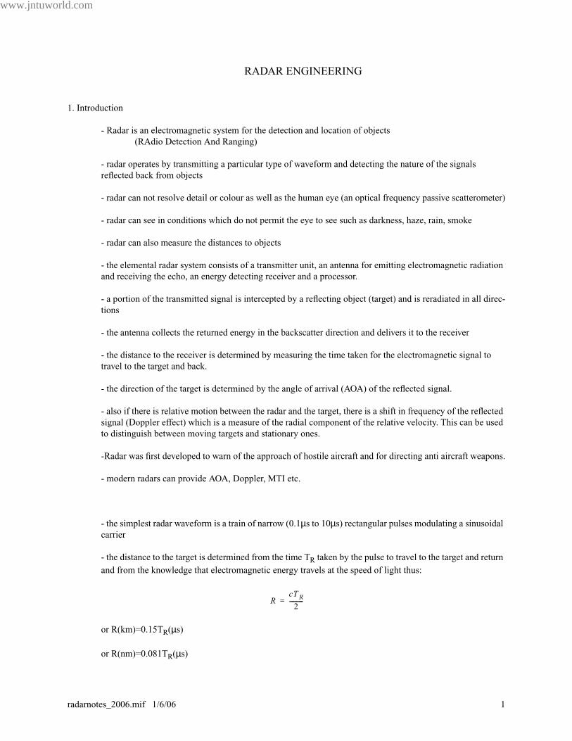
- the simplest radar waveform is a train of narrow (0.1µs to 10µs) rectangular pulses modulating a sinusoidal
carrier
- the distance to the target is determined from the time TR taken by the pulse to travel to the target and return
and from the knowledge that electromagnetic energy travels at the speed of light thus:
or R(km)=0.15TR(µs)
or R(nm)=0.081TR(µs)
RcTR
2----------=
www.jntuworld.com
radarnotes_2006.mif 1/6/06 1
97.460 PART II RADAR
www.jntuworld.com
JNTUWORLD
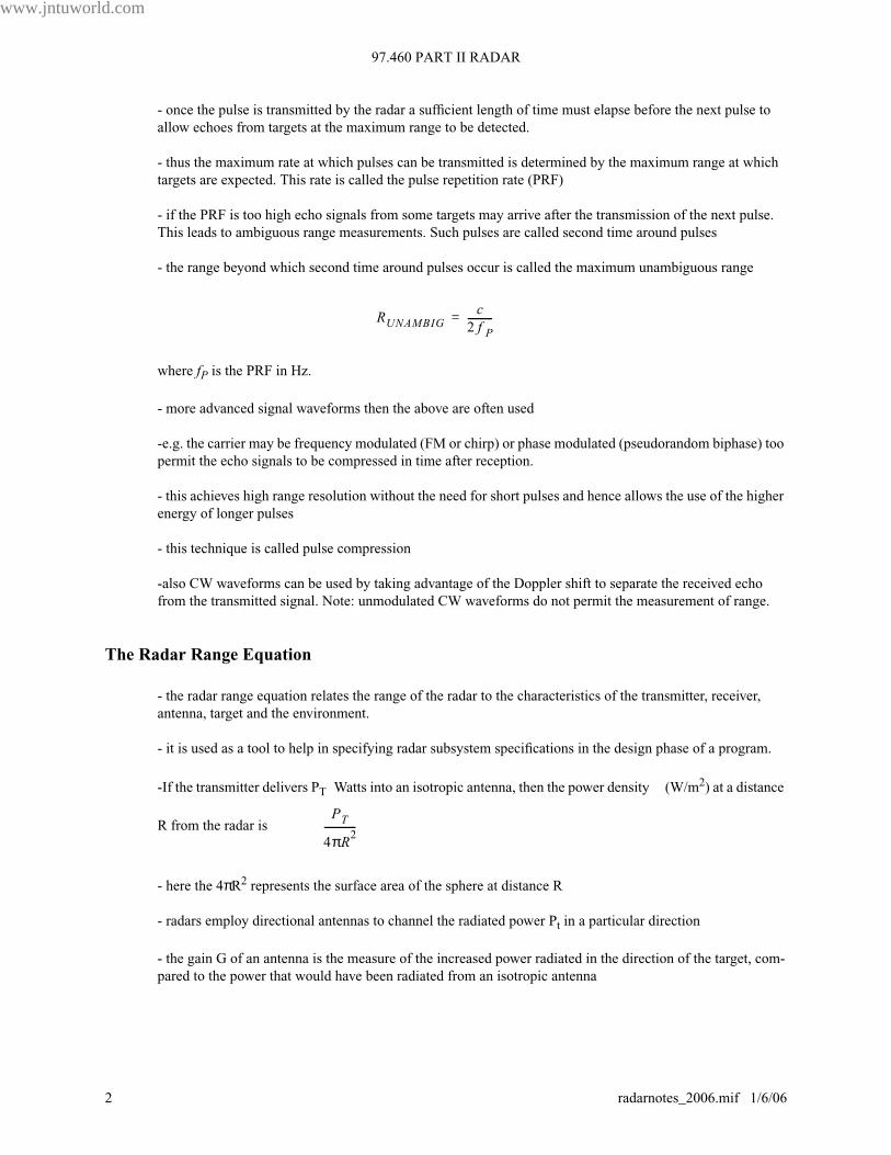
- once the pulse is transmitted by the radar a sufficient length of time must elapse before the next pulse to
allow echoes from targets at the maximum range to be detected.
- thus the maximum rate at which pulses can be transmitted is determined by the maximum range at which
targets are expected. This rate is called the pulse repetition rate (PRF)
- if the PRF is too high echo signals from some targets may arrive after the transmission of the next pulse.
This leads to ambiguous range measurements. Such pulses are called second time around pulses
- the range beyond which second time around pulses occur is called the maximum unambiguous range
where fP is the PRF in Hz.
- more advanced signal waveforms then the above are often used
-e.g. the carrier may be frequency modulated (FM or chirp) or phase modulated (pseudorandom biphase) too
permit the echo signals to be compressed in time after reception.
- this achieves high range resolution without the need for short pulses and hence allows the use of the higher
energy of longer pulses
- this technique is called pulse compression
-also CW waveforms can be used by taking advantage of the Doppler shift to separate the received echo
from the transmitted signal. Note: unmodulated CW waveforms do not permit the measurement of range.
The Radar Range Equation
- the radar range equation relates the range of the radar to the characteristics of the transmitter, receiver,
antenna, target and the environment.
- it is used as a tool to help in specifying radar subsystem specifications in the design phase of a program.
-If the transmitter delivers PT Watts into an isotropic antenna, then the power density (W/m2) at a distance
R from the radar is
- here the 4πR2 represents the surface area of the sphere at distance R
- radars employ directional antennas to channel the radiated power Pt in a particular direction
- the gain G of an antenna is the measure of the increased power radiated in the direction of the target, com-
pared to the power that would have been radiated from an isotropic antenna
RUNAMBIGc
2 f P----------=
PT
4πR2-------------
www.jntuworld.com
2 radarnotes_2006.mif 1/6/06
www.jntuworld.com
JNTUWORLD
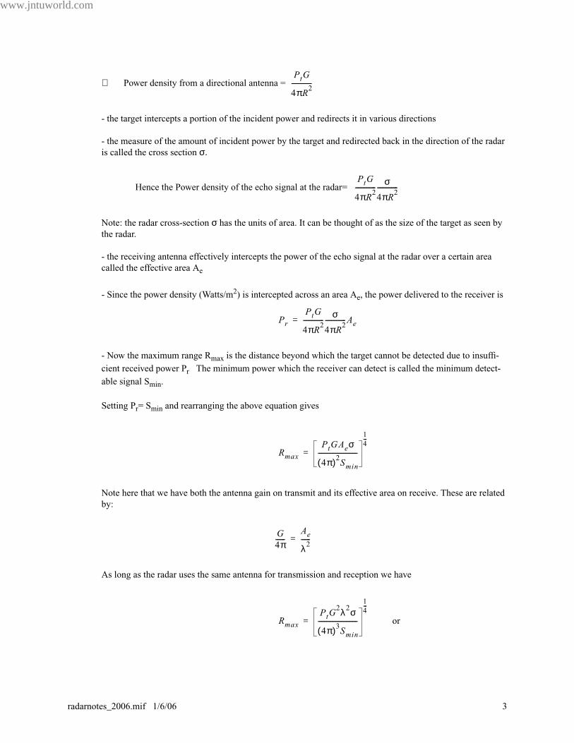
∴ Power density from a directional antenna =
- the target intercepts a portion of the incident power and redirects it in various directions
- the measure of the amount of incident power by the target and redirected back in the direction of the radar
is called the cross section σ.
Hence the Power density of the echo signal at the radar=
Note: the radar cross-section σ has the units of area. It can be thought of as the size of the target as seen by
the radar.
- the receiving antenna effectively intercepts the power of the echo signal at the radar over a certain area
called the effective area Ae
- Since the power density (Watts/m2) is intercepted across an area Ae, the power delivered to the receiver is
- Now the maximum range Rmax is the distance beyond which the target cannot be detected due to insuffi-
cient received power Pr The minimum power which the receiver can detect is called the minimum detect-
able signal Smin.
Setting Pr= Smin and rearranging the above equation gives
Note here that we have both the antenna gain on transmit and its effective area on receive. These are related
by:
As long as the radar uses the same antenna for transmission and reception we have
or
PtG
4πR2-------------
PtG
4πR2-------------
σ
4πR2-------------
PrPtG
4πR2-------------
σ
4πR2-------------Ae=
RmaxPtGAeσ
4π( )2Smin
-------------------------
1
4---
=
G4π------
Ae
λ2------=
RmaxPtG
2λ2σ
4π( )3Smin
-------------------------
1
4---
=
www.jntuworld.com
radarnotes_2006.mif 1/6/06 3
97.460 PART II RADAR
www.jntuworld.com
JNTUWORLD
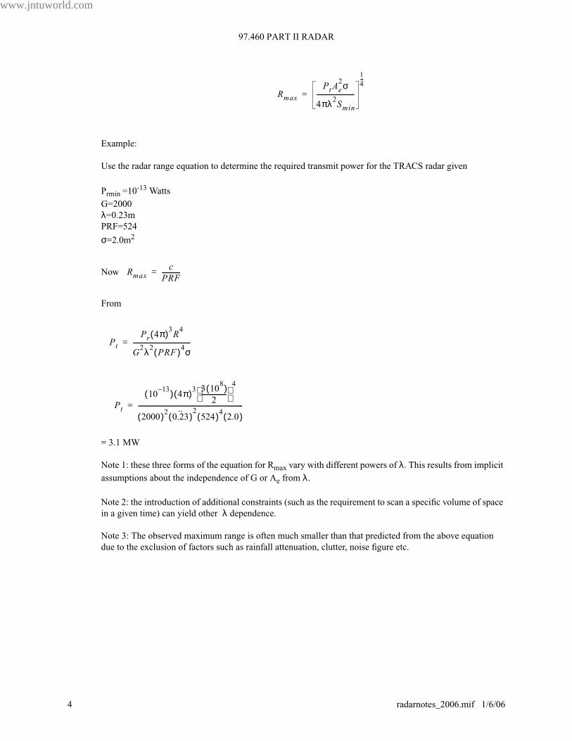
Example:
Use the radar range equation to determine the required transmit power for the TRACS radar given
Prmin =10-13 Watts
G=2000
λ=0.23m
PRF=524
σ=2.0m2
Now
From
= 3.1 MW
Note 1: these three forms of the equation for Rmax vary with different powers of λ. This results from implicit
assumptions about the independence of G or Ae from λ.
Note 2: the introduction of additional constraints (such as the requirement to scan a specific volume of space
in a given time) can yield other λ dependence.
Note 3: The observed maximum range is often much smaller than that predicted from the above equation
due to the exclusion of factors such as rainfall attenuation, clutter, noise figure etc.
RmaxPtAe
2σ
4πλ2Smin
------------------------
1
4---
=
Rmaxc
PRF------------=
PtPr 4π( )3
R4
G2λ2
PRF( )4σ-------------------------------------=
Pt
1013–( ) 4π( )3 3 10
8( )2
----------------
4
2000( )20.23˙( )
2524( )4
2.0( )-------------------------------------------------------------------=
www.jntuworld.com
4 radarnotes_2006.mif 1/6/06
www.jntuworld.com
JNTUWORLD
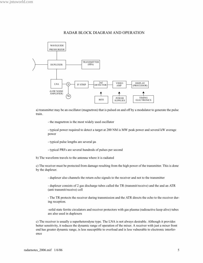
a) transmitter may be an oscillator (magnetron) that is pulsed on and off by a modulator to generate the pulse
train.
- the magnetron is the most widely used oscillator
- typical power required to detect a target at 200 NM is MW peak power and several kW average
power
- typical pulse lengths are several µs
- typical PRFs are several hundreds of pulses per second
b) The waveform travels to the antenna where it is radiated
c) The receiver must be protected from damage resulting from the high power of the transmitter. This is done
by the duplexer.
- duplexer also channels the return echo signals to the receiver and not to the transmitter
- duplexer consists of 2 gas discharge tubes called the TR (transmit/receive) and the and an ATR
(anti transmit/receive) cell
- The TR protects the receiver during transmission and the ATR directs the echo to the receiver dur-
ing reception.
-solid state ferrite circulators and receiver protectors with gas plasma (radioactive keep alive) tubes
are also used in duplexers
c) The receiver is usually a superheterodyne type. The LNA is not always desirable. Although it provides
better sensitivity, it reduces the dynamic range of operation of the mixer. A receiver with just a mixer front
end has greater dynamic range, is less susceptible to overload and is less vulnerable to electronic interfer-
ence
WAVEGUIDE
PRESSURIZER
DUPLEXER
TRANSMITTER(HPA)
LNA IF STRIP2nd
DETECTORVIDEO AMP
DISPLAY(PROCESSOR)
X
~BITE
POWERSUPPLIES
TIMINGELECTRONICS
RADAR BLOCK DIAGRAM AND OPERATION
(LOW NOISEAMPLIFIER)
www.jntuworld.com
radarnotes_2006.mif 1/6/06 5

97.460 PART II RADAR
www.jntuworld.com
JNTUWORLD
.
d) The mixer and Local Oscillator (LO) convert the RF frequency to the IF frequency.
- the IF is typically 300MHz, 140Mz, 60 MHz, 30 MHz with bandwidths of 1 MHz to 10 MHz.
- the IF strip should be designed to give a matched filter output. This requires its H(f) to maximize
the signal to noise power ratio at the output.
- this occurs if the |H(f)| (magnitude of the frequency response of the IF strip is equal to the signal
spectrum of the echo signal |S(f)|, and the ARG(H(f)) (phase of the frequency response) is the neg-
ative of the ARG(S(f)).
X
~
G
EFFECT OF LNA ON DYNAMIC RANGE
X
~
1dB compression
Si min
DRSi max
Noise Floor
LSi max
LSi min
DR
1dB compression, mixer
Si min
Si max
Noise FloorGNi+Ne
NiSi minG
1dB compression, mixer
Si max G
Si max GL
Noise FloorNoise Floor
L(GNi+Ne) Si minGL
DR
www.jntuworld.com
6 radarnotes_2006.mif 1/6/06
www.jntuworld.com
JNTUWORLD
i.e. H(f) and S(f) should be complex conjugates
- for radar with rectangular pulses, a conventional IF filter characteristic approximates a matched
filter if its bandwidth B and the pulse width τ satisfy the relationship
e) The pulse modulation is extracted by the second detector and amplified by video amplifiers to levels at
which they can be displayed (or A to D’d to a digital processor)
f) The display is usually a CRT; timing signals are applied to the display to provide zero range information.
Angle information is supplied from the pointing direction of the antenna.
- the most common type of CRT display is the plan position indicator (PPI) which maps the loca-
tion of the target in azimuth and range in polar coordinates
- the PPI is intensity modulated by the amplitude of the receiver output and the CRT electron beam
sweeps outward from the centre corresponding to range.
- Also the beam rotates in angle in synchronization with the antenna pointing angle.
- A B scope display uses rectangular coordinates to display range vs angle i.e. the x axis is angle
and the y axis is range.
- since both the PPI and B scopes use intensity modulation the dynamic range is limited
- An A scope plots target echo amplitude vs range on rectangular coordinates for some fixed direc-
tion. It is used primarily for tracking radar applications than for surveillance radar.
g) The simple diagram has left out many details such as
- AFC to compensate the receiver automatically for changes in the transmitter
- AGC
- Circuits in the receiver to reduce interference from other radars
- rotary joints in the transmission lines to allow for movement of the antenna
- MTI (moving target indicator) circuits to discriminate between moving targets and unwanted sta-
tionary targets
- pulse compression to achieve the resolution benefits of a short pulse but with the energy benefits
of a long pulse.
- monopulse tracking circuits for sensing the angular location of a moving target and allowing the
antenna to lock on and track the target automatically
- monitoring devices to monitor transmitter pulse shape, power load and receiver sensitivity
- built in test equipment (BITE) for locating equipment failures so that faulty circuits can be
replaced quickly
Bτ 1≈
www.jntuworld.com
radarnotes_2006.mif 1/6/06 7
97.460 PART II RADAR
www.jntuworld.com
JNTUWORLD
h) Instead of displaying the raw video output directly on the CRT, it might be digitized and processed and
then displayed. This consists of:
- quantizing the echo level at range-azimuth resolution cells
- adding (integrating) the echo level in each cell
- establishing a threshold level that permits only the strong outputs due to target echoes to pass
while rejecting noise
- maintaining the tracks (trajectories) of each target
- displaying the processed information
This process is called automatic tracking and detection (ATD) in a surveillance radar
i) Antennas
- the most common form of radar antenna is a reflector with parabolic shape, fed from a point
source (horn) at its focus
- the beam is scanned in space by mechanically pointing the antenna
- phased array antennas are sometimes used. Her the beam is scanned by varying the phase of the
array elements electrically
Radar Frequencies
- most radars operate between 220 MHz and 35 Ghz
- special purpose radars operate out side of this range
Skywave HF-OTH (over the horizon) can operate as low as 4 MHz
Groundwave HF radars operate as low as 2 MHz
millimeter radars operate up to 95 GHz
laser radars (lidars) operate in IR and visible spectrum
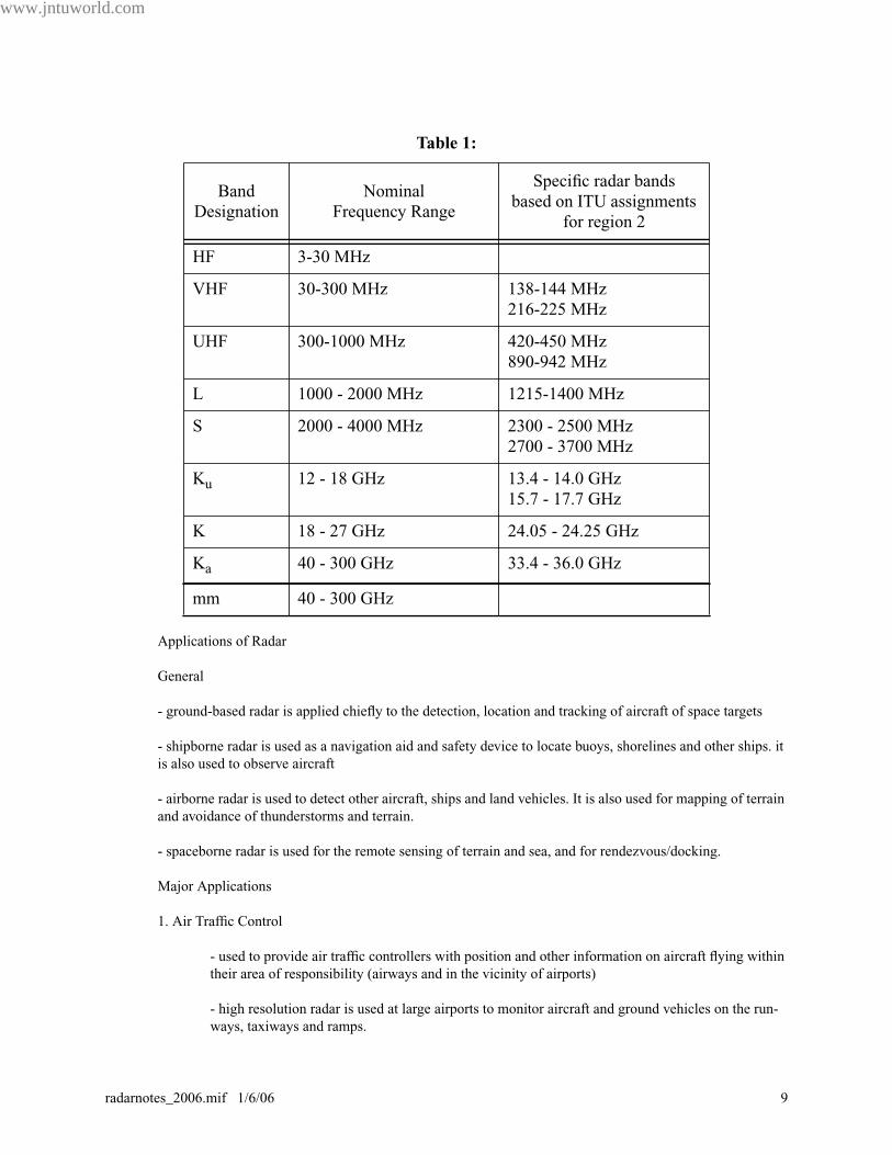
The radar frequency letter-band nomenclature is shown in the table. Note that the frequency assign-
ment to the latter band radar (e.g. L band radar) is much smaller than the complete range of fre-
quencies assigned to the letter band
www.jntuworld.com
8 radarnotes_2006.mif 1/6/06
www.jntuworld.com
JNTUWORLD
Applications of Radar
General
- ground-based radar is applied chiefly to the detection, location and tracking of aircraft of space targets
- shipborne radar is used as a navigation aid and safety device to locate buoys, shorelines and other ships. it
is also used to observe aircraft
- airborne radar is used to detect other aircraft, ships and land vehicles. It is also used for mapping of terrain
and avoidance of thunderstorms and terrain.
- spaceborne radar is used for the remote sensing of terrain and sea, and for rendezvous/docking.
Major Applications
1. Air Traffic Control
- used to provide air traffic controllers with position and other information on aircraft flying within
their area of responsibility (airways and in the vicinity of airports)
- high resolution radar is used at large airports to monitor aircraft and ground vehicles on the run-
ways, taxiways and ramps.
Table 1:
Band
Designation
Nominal
Frequency Range
Specific radar bands
based on ITU assignments
for region 2
HF 3-30 MHz
VHF 30-300 MHz 138-144 MHz
216-225 MHz
UHF 300-1000 MHz 420-450 MHz
890-942 MHz
L 1000 - 2000 MHz 1215-1400 MHz
S 2000 - 4000 MHz 2300 - 2500 MHz
2700 - 3700 MHz
Ku 12 - 18 GHz 13.4 - 14.0 GHz
15.7 - 17.7 GHz
K 18 - 27 GHz 24.05 - 24.25 GHz
Ka 40 - 300 GHz 33.4 - 36.0 GHz
mm 40 - 300 GHz
www.jntuworld.com
radarnotes_2006.mif 1/6/06 9

97.460 PART II RADAR
www.jntuworld.com
JNTUWORLD
- GCA (ground controlled approach) or PAR (precision approach radar) provides an operator with
high accuracy aircraft position information in both the vertical and horizontal. The operator uses
this information to guide the aircraft to a landing in bad weather.
- MLS (microwave landing system) and ATC radar beacon systems are based on radar technology
2. Air Navigation
- weather avoidance radar is used on aircraft to detect and display areas of heavy precipitation and
turbulence.
- terrain avoidance and terrain following radar (primarily military)
- radio altimeter (FM/CW or pulse)
- doppler navigator
- ground mapping radar of moderate resolution sometimes used for navigation
3. Ship Safety
- these are one of the least expensive, most reliable and largest applications of radar
- detecting other craft and buoys to avoid collision
- automatic detection and tracking equipment (also called plot extractors) are available with these
radars for collision avoidance
- shore based radars of moderate resolution are used from harbour surveillance and as an aid to nav-
igation
4. Space
- radars are used for rendezvous and docking and was used for landing on the moon
- large ground based radars are used for detection and tracking of satellites
- satellite-borne radars are used for remote sensing (SAR, synthetic aperture radar)
5. Remote Sensing
- used for sensing geophysical objects (the environment)
- radar astronomy - to probe the moon and planets
- ionospheric sounder (used to determine the best frequency to use for HF communications)
- earth resources monitoring radars measure and map sea conditions, water resources, ice cover,
agricultural land use, forest conditions, geological formations, environmental pollution
(Synthetic Aperture Radar, SAR and Side Looking Airborne Radar SLAR)
www.jntuworld.com
10 radarnotes_2006.mif 1/6/06

www.jntuworld.com
JNTUWORLD
6. Law Enforcement
- automobile speed radars
- intrusion alarm systems
7. Military
- surveillance
- navigation
- fire control and guidance of weapons
2. The Radar Range Equation
From page 3 we have
(2.1)
All of the parameters are controllable by the radar designer except for the target cross section σ.
In practice the simple range equation does not predict range performance accurately. The actual
range may be only half of that predicted.
This due, in part, to the failure to include various losses
It is also due to the statistical nature of several parameters such as Smin, σ, and propagation losses
Because of the statistical nature of these parameters, the range is described by the probability that
the radar will detect a certain type of target at a certain distance.
2.2 Minimum detectable Signal
The ability of the radar receiver to detect a weak echo is limited by the noise energy that occupies
the same spectrum as the signal
Detection is based on establishing a threshold level at the output of the receiver.
If the receiver output exceeds the threshold, a signal is assumed to be present
RmaxPtAe
2σ
4πλ2Smin
------------------------
1
4---
=
www.jntuworld.com
radarnotes_2006.mif 1/6/06 11
97.460 PART II RADAR
www.jntuworld.com
JNTUWORLD
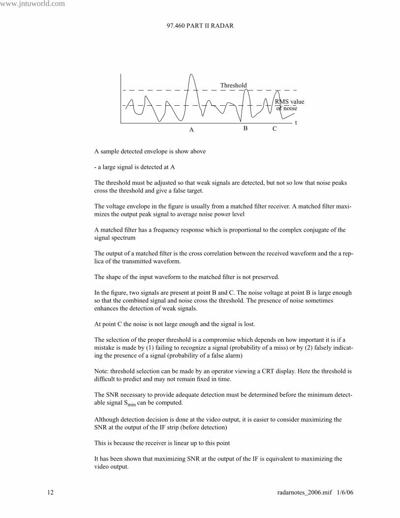
A sample detected envelope is show above
- a large signal is detected at A
The threshold must be adjusted so that weak signals are detected, but not so low that noise peaks
cross the threshold and give a false target.
The voltage envelope in the figure is usually from a matched filter receiver. A matched filter maxi-
mizes the output peak signal to average noise power level
A matched filter has a frequency response which is proportional to the complex conjugate of the
signal spectrum
The output of a matched filter is the cross correlation between the received waveform and the a rep-
lica of the transmitted waveform.
The shape of the input waveform to the matched filter is not preserved.
In the figure, two signals are present at point B and C. The noise voltage at point B is large enough
so that the combined signal and noise cross the threshold. The presence of noise sometimes
enhances the detection of weak signals.
At point C the noise is not large enough and the signal is lost.
The selection of the proper threshold is a compromise which depends on how important it is if a
mistake is made by (1) failing to recognize a signal (probability of a miss) or by (2) falsely indicat-
ing the presence of a signal (probability of a false alarm)
Note: threshold selection can be made by an operator viewing a CRT display. Here the threshold is
difficult to predict and may not remain fixed in time.
The SNR necessary to provide adequate detection must be determined before the minimum detect-
able signal Smin can be computed.
Although detection decision is done at the video output, it is easier to consider maximizing the
SNR at the output of the IF strip (before detection)
This is because the receiver is linear up to this point
It has been shown that maximizing SNR at the output of the IF is equivalent to maximizing the
video output.
Threshold
RMS valueof noise
A B Ct
www.jntuworld.com
12 radarnotes_2006.mif 1/6/06

www.jntuworld.com
JNTUWORLD
Receiver Noise
Noise is unwanted EM energy which interferes with the ability of the receiver to detect wanted sig-
nals.
Noise may be generated in the receiver or may enter the receiver via the antenna
One component of noise which is generated in the receiver is thermal (or Johnson) noise.
Noise power (Watts) = kTBn
where k = Boltzmann’s constant =1.38 x 10⁻²³ J/deg
T = degrees Kelvin
Bn = noise bandwidth
Note: Bn is not the 3 dB bandwidth but is given by:
here f0 is the frequency of maximum response
i.e. Bn is the width of an ideal rectangular filter whose response has the same area as the
filter or amplifier in question
Note: for many radars Bn is approximately equal to the 3 dB bandwidth (which is easier to
determine)
Note: a receiver with a reactive input (e.g. a parametric amplifier) need not have any ohmic loss and
hence all thermal noise is due to the antenna and transmission line preceding the antenna.
The noise power in a practical receiver is often greater than can be accounted for by thermal noise.
This additional noise is created by other mechanisms than thermal agitation.
The total noise can be considered to be equal to thermal noise power from an ideal receiver multi-
plied by a factor called the noise figure Fn (sometimes NF)
= Noise out of a practical receiver/Noise out of an ideal receiver at T0
here Ga is the gain of the receiver
Note: the receiver bandwidth Bn is that of the IF amplifier in most receivers
Since and
Bn
H f( ) 2fd
∞–
∞
∫H f
0( ) 2
---------------------------------=
FnN
0
kT0Bn( )Ga
----------------------------=
Ga
SoSi-----= Ni kT
0Bn=
www.jntuworld.com
radarnotes_2006.mif 1/6/06 13

97.460 PART II RADAR
www.jntuworld.com
JNTUWORLD
we have
rearranging gives:
Now Smin is that value of Si corresponding to the minimum output SNR: (So/No) necessary for
detection
hence (2.6)
substituting 2.6 into the radar range equation (eqn 2.1) yields
(2.7)
Probability Density Function (PDF)
Consider the variable x as representing a typical measured value of a random process such as a
noise voltage.
divide the continuous range of values of x into small equal segments of length ∆x, and count the
number of times that x falls into each interval
The PDF p(x) is than defined as:
p(x) = lim (No of values in range ∆x at x)
∆x → 0 N
N → ∞
where N is the total number of values
The probability that a particular measured value lies within width dx centred at x is p(x)dx
also the probability that a value lies between x1 and x2 is
Note: PDF is always positive by definition
FnSi N i⁄S
0N
0⁄
-----------------=
SikT
0BnFnSoN
0
------------------------------=
Smin kT0BnFn
S0
N0
-------
min=
Rmax4 PtGAeσ
4π( )2kT
0BnFn S0
N0
⁄( )min
--------------------------------------------------------------------=
P x1
x x2
< <( ) p x( ) xd
x1
x2
∫=
www.jntuworld.com
14 radarnotes_2006.mif 1/6/06
www.jntuworld.com
JNTUWORLD
also
The average value of a variable function Φ(x) of a random variable x is:
hence the average value, or mean of x is
also the mean square value is
m1 and m2 are called the first and second moments of the random variable x.
Note: if x represents current, then m1 is the DC component and m2 multiplied by the resistance
gives the mean power.
Variance is defined as
=m2 - m21
Variance is also called the second central moment
if x represents current, µ2 multiplied by the resistance gives the mean power of the AC component.
standard deviation, σ is defined as the square root of the variance. This is the RMS value of the AC
component.
Uniform Probability Density Function
K, a < x < a + b
p(x)= 0 x < a, x > a+b
example of a uniform probability distribution is the phase of a random sine wave relative
to a particular origin of time.
p x( ) xd
∞–
∞
∫ 1=
Φ x( )⟨ ⟩ ave Φ x( ) p x( ) xd
∞–
∞
∫=
x⟨ ⟩ ave xp x( ) xd
∞–
∞
∫ m1
= =
x2⟨ ⟩ ave x
2p x( ) xd
∞–
∞
∫ m2
= =
µ2
σ2x m
1–( )2⟨ ⟩ ave x m
1–( )2
p x( ) xd
∞–
∞
∫= = =
www.jntuworld.com
radarnotes_2006.mif 1/6/06 15
97.460 PART II RADAR
www.jntuworld.com
JNTUWORLD
the constant K is found from the following
hence for the phase of a random sine wave
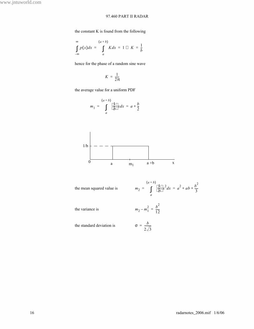
the average value for a uniform PDF
the mean squared value is
the variance is
the standard deviation is
p x( ) xd
∞–
∞
∫ K xd
a
a b+( )
∫ 1 K⇒ 1
b---= = =
K 1
2π------=
m1
1
b---
x xd
a
a b+( )
∫ a b2---+= =
a a +b
1/b
m1x0
m2
1
b---
x2xd
a
a b+( )
∫ a2
ab b2
3-----+ += =
m2
m1
2– b
2
12------=
σ b
2 3----------=
www.jntuworld.com
16 radarnotes_2006.mif 1/6/06

www.jntuworld.com
JNTUWORLD
Gaussian (Normal) PDF)
an example of normal PDF is thermal noise
we have for the Normal PDF
m1 = x0
m2 = x20 + σ2
σ2 = m2 - m12
Central Limit Theorem:
The PDF of the sum of a large number of independent, identically distributed random
quantities approaches the Normal PDF regardless of what the individual distribution might
be, provided that the contribution of any one quantity is not comparable with the resultant
of all the others
For the Normal distribution, no matter how large a value of x we may choose, there is always a
finite probability of finding a greater value
Hence if noise at the input to a threshold detector is normally distributed there is always a chance
for a false alarm.
Rayleigh PDF
x ≥ 0
examples of a Rayleigh PDF are the envelope of noise output from a narrowband band pass filter
(IF filter in superheterodyne receiver), also the cross section fluctuations of certain types of targets
and also many kinds of clutter and weather echoes.
p x( ) 1
2πσ2-----------------
x x0
–( )2–
2σ2-------------------------
exp=
x0
1/√2πσ
x
p(x)
p x( ) x
x2⟨ ⟩ ave
------------------x
2
2 x2⟨ ⟩ ave
----------------------–
exp=
www.jntuworld.com
radarnotes_2006.mif 1/6/06 17
97.460 PART II RADAR
www.jntuworld.com
JNTUWORLD
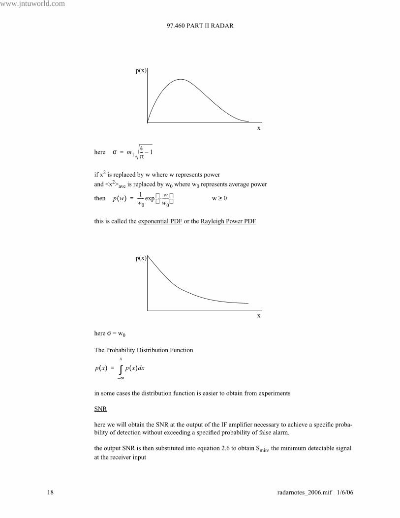
here
if x2 is replaced by w where w represents power
and <x2>ave is replaced by w0 where w0 represents average power
then w ≥ 0
this is called the exponential PDF or the Rayleigh Power PDF
here σ = w0
The Probability Distribution Function
in some cases the distribution function is easier to obtain from experiments
SNR
here we will obtain the SNR at the output of the IF amplifier necessary to achieve a specific proba-
bility of detection without exceeding a specified probability of false alarm.
the output SNR is then substituted into equation 2.6 to obtain Smin, the minimum detectable signal
at the receiver input
p(x)
x
σ m1
4
π--- 1–=
p w( ) 1
w0
------ww
0
------– exp=
p(x)
x
p x( ) p x( ) xd
∞–
x
∫=
www.jntuworld.com
18 radarnotes_2006.mif 1/6/06
www.jntuworld.com
JNTUWORLD
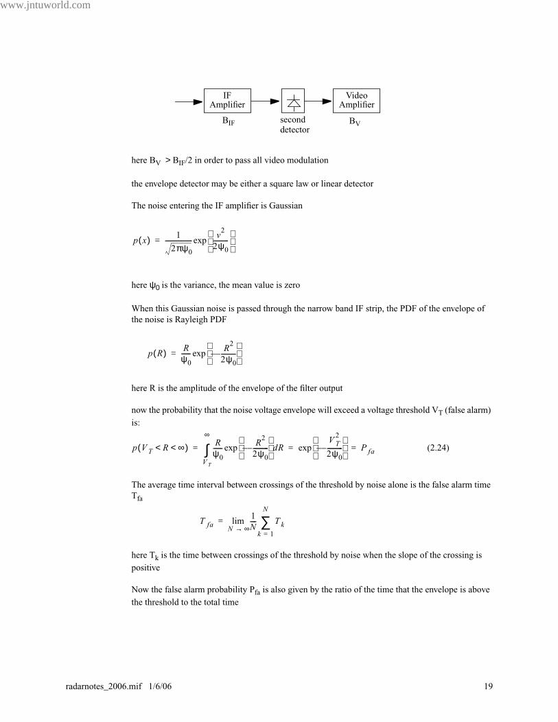
here BV > BIF/2 in order to pass all video modulation
the envelope detector may be either a square law or linear detector
The noise entering the IF amplifier is Gaussian
here ψ0 is the variance, the mean value is zero
When this Gaussian noise is passed through the narrow band IF strip, the PDF of the envelope of
the noise is Rayleigh PDF
here R is the amplitude of the envelope of the filter output
now the probability that the noise voltage envelope will exceed a voltage threshold VT (false alarm)
is:
(2.24)
The average time interval between crossings of the threshold by noise alone is the false alarm time
Tfa
here Tk is the time between crossings of the threshold by noise when the slope of the crossing is
positive
Now the false alarm probability Pfa is also given by the ratio of the time that the envelope is above
the threshold to the total time
IFAmplifier
VideoAmplifier
BIF BVsecond
detector
p x( ) 1
2πψ0
------------------v
2
2ψ0
----------
exp=
p R( ) Rψ
0
------R
2
2ψ0
----------––
exp=
p VT R ∞< <( ) Rψ
0
------
VT
∞
∫ R2
2ψ0
----------––
dRexpVT
2
2ψ0
----------––
exp P fa= = =
T fa1
N----
N ∞→lim Tk
k 1=
N
∑=
www.jntuworld.com
radarnotes_2006.mif 1/6/06 19
97.460 PART II RADAR
www.jntuworld.com
JNTUWORLD
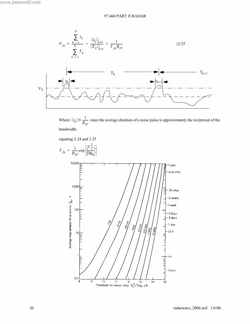
(2.25
Where since the average duration of a noise pulse is approximately the reciprocal of the
bandwidth.
equating 2.24 and 2.25
P fa
tkk 1=
N
∑
Tkk 1=
N
∑-----------------
tk⟨ ⟩ave
T k⟨ ⟩ave
-------------------1
T faBIF------------------= = =
VT
tk tk+1
TkTk+1
tk⟨ ⟩ 1
BIF---------≈
T fa1
BIF---------
VT2
2ψ0
----------
exp=
www.jntuworld.com
20 radarnotes_2006.mif 1/6/06

www.jntuworld.com
JNTUWORLD
Example:
for BIF = 1 MHz and required false alarm rate of 15 minutes, equation 2.25 gives
Note: the false alarm probabilities of practical radars are quite small. This is due to their narrow
bandwidth
Note: False alarm time Tfa is very sensitive to variations in the threshold level VT due to the expo-
nential relationship.
Example: for BIF = 1 MHz we have the following:
Note: If the receiver is gated off for part of the time (e.g. during transmission interval) the Pfa will
be increased by the fraction of the time that the receiver is not on. This assumes that Tfa remains
constant. The effect is usually negligible.
We now consider a sine wave signal of amplitude A present along with the noise at the input to the
IF strip.
Here the output of the envelope detector has a Rice PDF which is given by:
2.27
where I0(Z) is the modified Bessel function of zero order and argument Z
now
for Z large
Note: when A = 0 equation 2.27 reduces to the PDF from noise alone
The probability of detection Pd is the probability that the envelope will exceed VT
VT2/2ψ0 Tfa
12.95 dB 6 min
14.72 dB 10,000 hours
P fa1
15( ) 60( ) 106⋅ ⋅
--------------------------------------- 1.11x10⁹–
= =
p R( ) Rψ
0
------R
2A
2+
2ψ0
-------------------–
I0
RAψ
0
------- exp=
I0Z( ) e
Z
2πZ-------------- 1
1
8Z------- …+ +
≈
Pd p R( ) Rd
VT
∞
∫=
www.jntuworld.com
radarnotes_2006.mif 1/6/06 21
97.460 PART II RADAR
www.jntuworld.com
JNTUWORLD
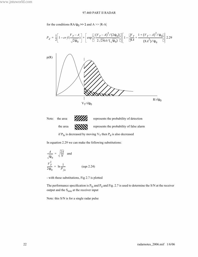
for the conditions RA/ψ0 >> 1and A >> |R-A|
2.29
Note: the area represents the probability of detection
the area represents the probability of false alarm
if Pfa is decreased by moving VT then Pd is also decreased
In equation 2.29 we can make the following substitutions:
and
(eqn 2.24)
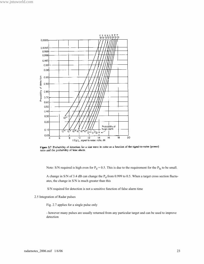
- with these substitutions, Fig 2.7 is plotted
The performance specification is Pfa and Pd and Fig. 2.7 is used to determine the S/N at the receiver
output and the Smin at the receiver input
Note: this S/N is for a single radar pulse
Pd1
2--- 1 er f
V T A–
2ψ0
-----------------( )–VT A–( )2
2ψ0
( )⁄
2 2πA ψ0
( )⁄--------------------------------------------–
exp 1VT4A-------
1 VT A–( )2 ψ0
⁄+
8A2( ) ψ
0⁄
---------------------------------------------+
–+=
p(R)
VT/√ψ0
R/√ψ0
A
ψ0
-----------2SN------=
VT2
2ψ0
----------1
P fa---------ln=
www.jntuworld.com
22 radarnotes_2006.mif 1/6/06
www.jntuworld.com
JNTUWORLD
Note: S/N required is high even for Pd = 0.5. This is due to the requirement for the Pfa to be small.
A change in S/N of 3.4 dB can change the Pd from 0.999 to 0.5. When a target cross section fluctu-
ates, the change in S/N is much greater than this
S/N required for detection is not a sensitive function of false alarm time
2.5 Integration of Radar pulses
Fig. 2.7 applies for a single pulse only
- however many pulses are usually returned from any particular target and can be used to improve
detection
www.jntuworld.com
radarnotes_2006.mif 1/6/06 23
97.460 PART II RADAR
www.jntuworld.com
JNTUWORLD
- the number of pulses nB as the antenna scans is
where θB = antenna beam width (deg)
fP = PRF (Hz)
= antenna scan rate (deg/sec)
ωm = antenna scan rate (rpm)
Example: For a ground based search radar having
θB = 1.5 ˚
fP = 300 Hz
= 30˚/s (ωm = 5 rpm)
determine the number of hits from a point target in each scan
nB = 15
- The process of summing radar echoes to improve detection is called integration
- all integration techniques employ a storage device
- the simplest integration method is the CRT display combined with the integrating proper-
ties of the eye and brain of the operator.
- for electronic integration, the function can be accomplished in the receiver either before
the second detector (in the IF) or after the second detector (in the video)
- integration before detection is called predetection or coherent detection
- integration after detection is called postdetection or noncoherent integration
- predetection integration requires the phase of the echo signal to be preserved
- postdetection integration can not preserve RF phase
- for predetection SNRintegrated = n SNRi
where SNRi is the SNR for a single pulse
and n is the number of pulses integrated
- for postdetection, the integrated SNR is less than the above since some of the energy is
converted to noise in the nonlinear second detector
- postdetection integration, however, is easier to implement
- integration efficiency is defined as
where = value of SNR of a single pulse required to produce a given probability of detec-
tion
nBθB f P
θS-------------
θB f P6ωm-------------= =
θS
θS
Ei n( )S N⁄( )
1
n S N⁄( )n----------------------=
S N⁄( )1
www.jntuworld.com
24 radarnotes_2006.mif 1/6/06

www.jntuworld.com
JNTUWORLD
and is the value of SNR per pulse required to produce the same probability of detection
when n pulses are integrated.
Note: for postdetection integration, the integration improvement factor is Ii = nEi(n)
for ideal postdetection, Ei(n) = 1 and hence the integration improvement factor is n
Examples of Ii are given in Fig. 2.8a from data by Marcum
- note that Ii is not sensitive to either Pd or Pfa
- we can also develop the integration loss as
this is shown in Fig 2.8b
- the parameter nf in Fig 2.8 is called the false alarm number which is defined as the average num-
ber of possible decisions between false alarms
nf = [no. of range intervals/pulse][no. of pulse periods/sec][false alarm rate]
= [TP/τ][fP][Tfa]
here TP = PRI (pulse repetition interval)
fP = PRF
Thus nf = Tfa /τ
≈ TfaB
≈ 1/Pfa
Note: for a radar with pulse width τ, there are B = 1/τ possible decisions per second on the presence
of a target
- if n pulses are integrated before a target decision is made, then there are B/n possible decisions/
sea.
- hence the false alarm probability is n times as great
Note: this does not mean that there will be more false alarms since it is the rate of detection-deci-
sions is reduced, not the average time between false alarms
- hence Tfa is more meaningful than Pfa
Note: some authors use a false alarm number nf’ = nf/n
caution should be used in computations for SNR as a function of Pfa and Pd
- Fig. 2.8a shows that for a few pulses integrated post detection, there is not much difference from a
perfect predetection integrator.
S N⁄( )n
Li 101
Ei n( )-------------log=
www.jntuworld.com
radarnotes_2006.mif 1/6/06 25

97.460 PART II RADAR
www.jntuworld.com
JNTUWORLD
www.jntuworld.com
26 radarnotes_2006.mif 1/6/06
www.jntuworld.com
JNTUWORLD
- when there are many pulses integrated (small S/N per pulse) the difference is pronounced.
- the radar equation with n pulses integrated is
2.23
here (S/N)n is the SNR of one of n equal pulses that are integrated to produce the required Pd for a
specified Pfa
using equation 2.31 in 2.32
here (S/N)1 is found from Fig. 2.7 and nEi(n) is found from Fig 2.8a.
some postdetection integrators use a weighting of the integrated pulses. These integrators include
the recirculating delay line, the LPF, the storage tube and some algorithms in digital integration.
- if an “exponential” weighting of the integrated pulses is used then the voltage out of the integrator
is
here Vi is the voltage amplitude of the ith pulse and exp(-γ) is the attenuation per pulse
- for this weighting, an efficiency factor ρ can be calculated which is the ratio of the average S/N for
the exponential integrator to the average S/N for the uniform integrator:
for a dumped integrator
also
for a continuous integrator
Note: Maximum efficiency for a dumped integrator corresponds to γ =0
Maximum efficiency for a continuous integrator corresponds to nγ =1.257
2.7 Radar Cross Section of Targets
Cross-section: The fictional area intercepting that amount of power which, when scattered equally
in all directions, produces an echo at the radar that is equal to that actually received.
Rmax4 PtGAeσ
4π( )2kT
0BnFn S N⁄( )n
----------------------------------------------------------=
Rmax4 PtGAeσnEi n( )
4π( )2kT
0BnFn S N⁄( )
1
----------------------------------------------------------=
V V i i 1–( )γ–[ ]exp
i 1=
N
∑=
ρ
nγ2
------ tanh
nγ2---
tanh
-----------------------=
ρ 1 nγ–( )exp–[ ] 2
nγ2---
tanh
----------------------------------------=
www.jntuworld.com
radarnotes_2006.mif 1/6/06 27

97.460 PART II RADAR
www.jntuworld.com
JNTUWORLD
σ = power reflected towards the source/unit solid angle
incident power density/4π
=
where R = range
Er= reflected field strength at radar
Ei = incident field strength at target
Note: for most targets such as aircraft. ships and terrain, the σ does not bear a simple relationship to
the physical area
- EM scattered field: is the difference between the total field in the presence of an object and the
field that would exist if the object were absent
- EM diffracted field: is the total field in the presence of the object
Note: for radar backscatter, the two fields are the same (since the transmitted field has disappeared
by the time the received field appears)
- the σ can be calculated using Maxwell’s equations only for simple targets such as the sphere (Fig.
2.9)
-when (the Rayleigh region), the scattering from a sphere can be used for modelling rain-
drops
4πR2
R ∞→lim
ErEi------
2
2πaλ
---------- 1«
www.jntuworld.com
28 radarnotes_2006.mif 1/6/06
www.jntuworld.com
JNTUWORLD
- since σ varies as λ-4 in the Rayleigh region, rain and clouds are invisible for long wavelength
radars
- the usual radar targets are much larger than raindrops and hence the long λ operation does not
reduce the target σ
-when the σ approaches the optical cross section πa2.
Note: in the Mie (resonance region) σ can actually be 5.6 dB greater than the optical value or 5.6
dB smaller.
Note: For a sphere the σ is not aspect sensitive as it is for all other objects, and hence can be used
fro calibrating a radar system.
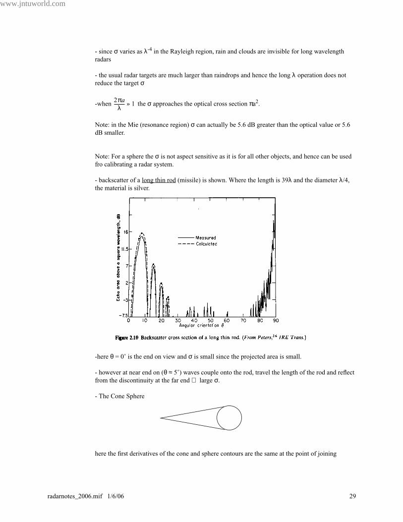
- backscatter of a long thin rod (missile) is shown. Where the length is 39λ and the diameter λ/4,
the material is silver.
-here θ = 0˚ is the end on view and σ is small since the projected area is small.
- however at near end on (θ ≈ 5˚) waves couple onto the rod, travel the length of the rod and reflect
from the discontinuity at the far end ⇒ large σ.
- The Cone Sphere
here the first derivatives of the cone and sphere contours are the same at the point of joining
2πaλ
---------- 1»
www.jntuworld.com
radarnotes_2006.mif 1/6/06 29
97.460 PART II RADAR
www.jntuworld.com
JNTUWORLD
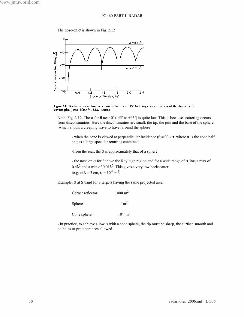
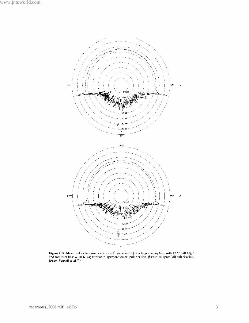
The nose-on σ is shown in Fig. 2.12
Note: Fig. 2.12. The σ for θ near 0˚ (-45˚ to +45˚) is quite low. This is because scattering occurs
from discontinuities. Here the discontinuities are small: the tip, the join and the base of the sphere
(which allows a creeping wave to travel around the sphere)
- when the cone is viewed at perpendicular incidence (θ = 90 - α, where α is the cone half
angle) a large specular return is contained
-from the rear, the σ is approximately that of a sphere
- the nose on σ for f above the Rayleigh region and for a wide range of α, has a max of
0.4λ2 and a min of 0.01λ2. This gives a very low backscatter
(e.g. at λ = 3 cm, σ = 10-4 m2.
Example: σ at S band for 3 targets having the same projected area:
Corner reflector: 1000 m2
Sphere 1m2
Cone sphere 10-3 m2
- In practice, to achieve a low σ with a cone sphere, the tip must be sharp, the surface smooth and
no holes or protuberances allowed.
www.jntuworld.com
30 radarnotes_2006.mif 1/6/06
www.jntuworld.com
JNTUWORLD
www.jntuworld.com
radarnotes_2006.mif 1/6/06 31
97.460 PART II RADAR
www.jntuworld.com
JNTUWORLD
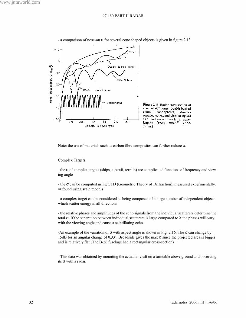
- a comparison of nose-on σ for several cone shaped objects is given in figure 2.13
Note: the use of materials such as carbon fibre composites can further reduce σ.
Complex Targets
- the σ of complex targets (ships, aircraft, terrain) are complicated functions of frequency and view-
ing angle
- the σ can be computed using GTD (Geometric Theory of Diffraction), measured experimentally,
or found using scale models
- a complex target can be considered as being composed of a large number of independent objects
which scatter energy in all directions
- the relative phases and amplitudes of the echo signals from the individual scatterers determine the
total σ. If the separation between individual scatterers is large compared to λ the phases will vary
with the viewing angle and cause a scintillating echo.
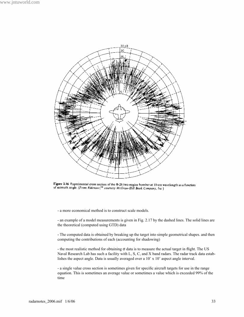
-An example of the variation of σ with aspect angle is shown in Fig. 2.16. The σ can change by
15dB for an angular change of 0.33˚. Broadside gives the max σ since the projected area is bigger
and is relatively flat (The B-26 fuselage had a rectangular cross-section)
- This data was obtained by mounting the actual aircraft on a turntable above ground and observing
its σ with a radar.
www.jntuworld.com
32 radarnotes_2006.mif 1/6/06
www.jntuworld.com
JNTUWORLD
- a more economical method is to construct scale models.
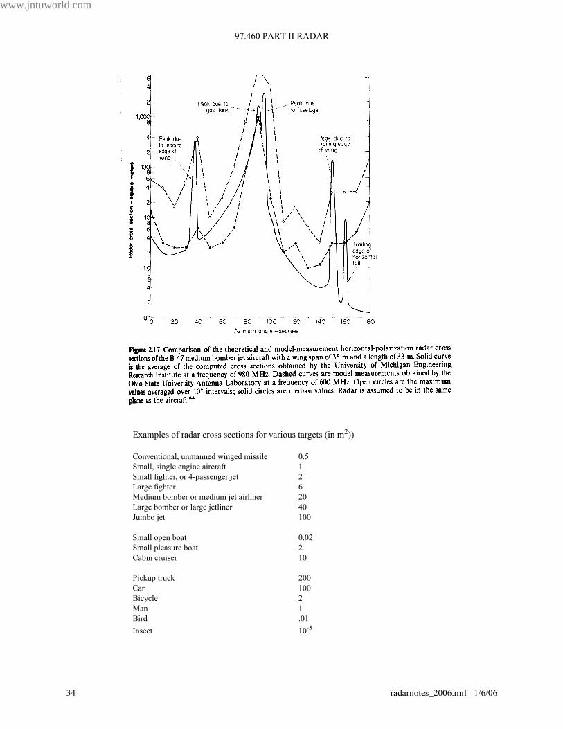
- an example of a model measurements is given in Fig. 2.17 by the dashed lines. The solid lines are
the theoretical (computed using GTD) data
- The computed data is obtained by breaking up the target into simple geometrical shapes. and then
computing the contributions of each (accounting for shadowing)
- the most realistic method for obtaining σ data is to measure the actual target in flight. The US
Naval Research Lab has such a facility with L, S, C, and X band radars. The radar track data estab-
lishes the aspect angle. Data is usually averaged over a 10˚ x 10˚ aspect angle interval.
- a single value cross section is sometimes given for specific aircraft targets for use in the range
equation. This is sometimes an average value or sometimes a value which is exceeded 99% of the
time
www.jntuworld.com
radarnotes_2006.mif 1/6/06 33
97.460 PART II RADAR
www.jntuworld.com
JNTUWORLD
Examples of radar cross sections for various targets (in m2))
Conventional, unmanned winged missile 0.5
Small, single engine aircraft 1
Small fighter, or 4-passenger jet 2
Large fighter 6
Medium bomber or medium jet airliner 20
Large bomber or large jetliner 40
Jumbo jet 100
Small open boat 0.02
Small pleasure boat 2
Cabin cruiser 10
Pickup truck 200
Car 100
Bicycle 2
Man 1
Bird .01
Insect 10-5
www.jntuworld.com
34 radarnotes_2006.mif 1/6/06

www.jntuworld.com
JNTUWORLD
Note: even though single values are given there can be large variations in actual σ for any target
e.g. the AD 4B, a propeller driven aircraft has a σ of 20 m2 at L band but its σ at VHF is about 100
m2 This is because at VHF the dimensions of the scattering objects are comparable to λ and pro-
duce a resonance effect
For large ships, an average cross section taken from port, starboard and quarter aspects yields
here σ is in m2
f is in MHz
D is ship displacement in kilotons
- this equation applies only to grazing angles i.e. as seen from the same elevation
- small boats 20 ft. to 30 ft. give σ(X band) approx 5 m2
40 ft. to 50 ft.
“ “ “ “ “ 10 m2
- automobiles give σ(X band) of approx 10 m2 to 200 m2
- human being gives σ as shown:
f (MHz) σ (m2)
410 0.033 - 2.33
1120 0.098 - 0.997
2890 0.140 - 1.05
4800 0.368 - 1.88
9375 0.495 - 1.22
2.8 Cross-Section Fluctuations
- the echo from a target in motion is almost never constant
- variations are caused by meteorological conditions, lobe structure of the antenna, equipment
instability and the variation in target cross section
- cross section of complex targets are sensitive to aspect
- one method of dealing with this is to select a lower bound of σ that is exceeded some specified
fraction of the time (0.95 or 0.99)
- this procedure results in conservative prediction of range
- alternatively, the PDF and the correlation properties with time may be used for a particular target
and type of trajectory
σmedian 52 f D3 2⁄
=
www.jntuworld.com
radarnotes_2006.mif 1/6/06 35

97.460 PART II RADAR
www.jntuworld.com
JNTUWORLD
- the PDF gives the probability of finding any value of σ between the values of σ and σ + dσ.
- the correlation function gives the degree of correlation of σ with time (i.e. number of pulses)
- the power spectral density of σ is also important in tracking radars.
- it is not usually practical to obtain experimental data for these functions
- it is more economical to assess the effects of fluctuating σ is to postulate a reasonable model for
the fluctuations and to analyze it mathematically
Swerling has done this for the detection probabilities of 5 types of target.
Case 1
echo pulses received from the target on any one scan are of constant envelope throughout
the entire scan, but are independent (uncorrelated) scan to scan
This case ignores the effect of antenna beam shape
the assumed PDF is:
σ ≥ 0
Case 2
echo pulses are independent from pulse to pulse instead of from scan to scan
Case 3
Same as case 1 except that the PDF is
Case 4
Same as case 2 except that the PDF is
Case 5
Nonfluctuating cross section
- The PDF assumed in cases 1 and 2 applies to complex targets consisting of many scatterers (in
practice 4 or more)
- The PDF assumed in cases 3 and 4 applies to targets represented by one large reflector with other
small reflectors
p σ( ) 1
σave-----------
σ–σave-----------
exp=
p σ( ) 1
σave-----------
σ–σave-----------
exp=
p σ( ) 4σ
σave2
-----------2σ–
σave-----------
exp=
p σ( ) 4σ
σave2
-----------2σ–
σave-----------
exp=
www.jntuworld.com
36 radarnotes_2006.mif 1/6/06

www.jntuworld.com
JNTUWORLD
- for all cases the value of σ to be substituted in the radar equation is σave
0 10 20 30 40 50 60 70 80 90 1000
0.005
0.01
0.015
0.02
0.025
0.03
0.035
0.04
0.045
0.05
PDF for Swerling 1 and 2 targets
average cross section = 20
0 10 20 30 40 50 60 70 80 90 1000
0.005
0.01
0.015
0.02
0.025
0.03
0.035
0.04
PDF for Swerling 3 and 4 targets
average cross section = 20
www.jntuworld.com
radarnotes_2006.mif 1/6/06 37

97.460 PART II RADAR
www.jntuworld.com
JNTUWORLD
- comparison of the five cases for a false alarm number nf = 108 is shown in Fig. 2.22
- when detection probability is large, all 4 cases in which σ is not constant require greater SNR
than the constant σ case (case 5)
- Note for Pd =0.95 we have
Case # S/N
1 16.8 dB/pulse
2 6.2 dB/pulse
This increase in S/N corresponds to a reduction in range by a factor of 1.84. Hence if the character-
istics of the target are not properly taken into account, the actual performance of the radar (for the
same value of σave) will not measure up to the predicted performance.
- also when Pd > 0.3, larger S/N is required when fluctuations are uncorrelated scan to scan (cases 1
& 3) than when fluctuations are uncorrelated pulse to pulse.
- this results since the larger the number of independent pulses integrated, the more likely the fluc-
tuations will average out ⇒ cases 2 & 4 will approach the nonfluctuating case.
www.jntuworld.com
38 radarnotes_2006.mif 1/6/06

www.jntuworld.com
JNTUWORLD
- Figures 2.23 and 2.24 may be used as corrections for probability of detection (Fig. 2.7)
www.jntuworld.com
radarnotes_2006.mif 1/6/06 39
97.460 PART II RADAR
www.jntuworld.com
JNTUWORLD
Procedure:
1) Find S/N from Fig. 2.7 corresponding to desired Pd and Pfa
2) From Fig. 2.23 find correction factor for either cases 1 and 2 or cases 3 and 4 to be
applied to S/N found in Step 1. The resulting (S/N)1 is that which would apply if detection
were based on a single pulse
3) If n pulses are integrated, The integration improvement factor Ii(n) is found from Fig.
2.24. The parameters (S/N)1 and nEi(n)=Ii(n) are substituted into the radar equation 2.33
along with σave.
Note: in Fig. 2.24 the integration improvement factor Ii(n) is sometimes greater than n. Here the S/
N required fro n=1 is larger than for the nonfluctuating target. The S/N per pulse will always be less
than that of the ideal predetection integrator.
Note: data in Fig. 2.23 and 2.24 are essentially independent of the false alarm number
(106<nf<1010)
Note: the PDF s for cases 1 &2 and # & 4 of the Swerling fluctuations are special cases of the Chi-
square distribution of degree 2m (also called the Gamma distribution)
σ > 0
Note: for target cross section models, 2m is not required to be an integer. It may be any positive real
number.
for cases 1 and 2, m=1
for cases 3 and 4, m=2
Note: For the Chi-square PDF
here is the standard deviation
and m1 is the mean value
Note: as m increases, the fluctuations become more constrained. With m = ∞, we have the nonfluc-
tuating target.
- the Chi-square distribution may not always fit observed data, but it is used for convenience
- it is described by two parameters σave and the number of degrees of freedom 2m.
p σ( ) mm 1–( )!σave
-------------------------------mσσave-----------
m 1– mσ–σave-----------
exp=
µ2
m1
---------- m
1
2---–
=
µ2
www.jntuworld.com
40 radarnotes_2006.mif 1/6/06
www.jntuworld.com
JNTUWORLD
- aircraft flying straight and level fit Chi-square distribution with m between 0.9 and 2, and with
σave varying 15 dB from min to max.
- the parameters of the fitted distribution vary with aspect angle, type of aircraft and frequency
- the value of m is near unity for all aspect angles except broadside which give a Rayleigh distribu-
tion with varying σave
- it is found that σave has more effect on the calculation of probability of detection than the value of
m.
- the Chi-square distribution also describes the cross section of shapes such as cylinders, cylinders
with fins (e.g. some satellites). Here m varies between 0.2 and 2 depending on the aspect angle.
- the Rice distribution is a better description of the cross section fluctuations of a target dominated
by a single scatterer than the Chi-square distribution with m=2.
- Here the Rice distribution is
where s is the ratio of the cross section of the single dominant scatterer to the total cross
section of the smaller scatterers
I0 is a modified Bessel function of zero order
Note: when s=1 the results using the Rice distribution approximate the Chi-square with m=2, for
small probabilities of detection
- The Log Normal distribution has been suggested for describing the cross sections of some satel-
lites, ships, cylinders, plates, arrays
σ > 0
where sd = standard deviation of
and σm = median of σ
also the ratio of the mean to median value of σ is ρ =
p σ( ) 1 s+σave----------- s–
σσave----------- 1 s+( )– I
02
σσave-----------s 1 s+( )
exp=
p σ( ) 1
2πsdσ--------------------
1
2sd2
--------σ
σm-------
ln 2
–exp=
σσm-------
ln
sd2
2-----
exp
www.jntuworld.com
radarnotes_2006.mif 1/6/06 41
97.460 PART II RADAR
www.jntuworld.com
JNTUWORLD
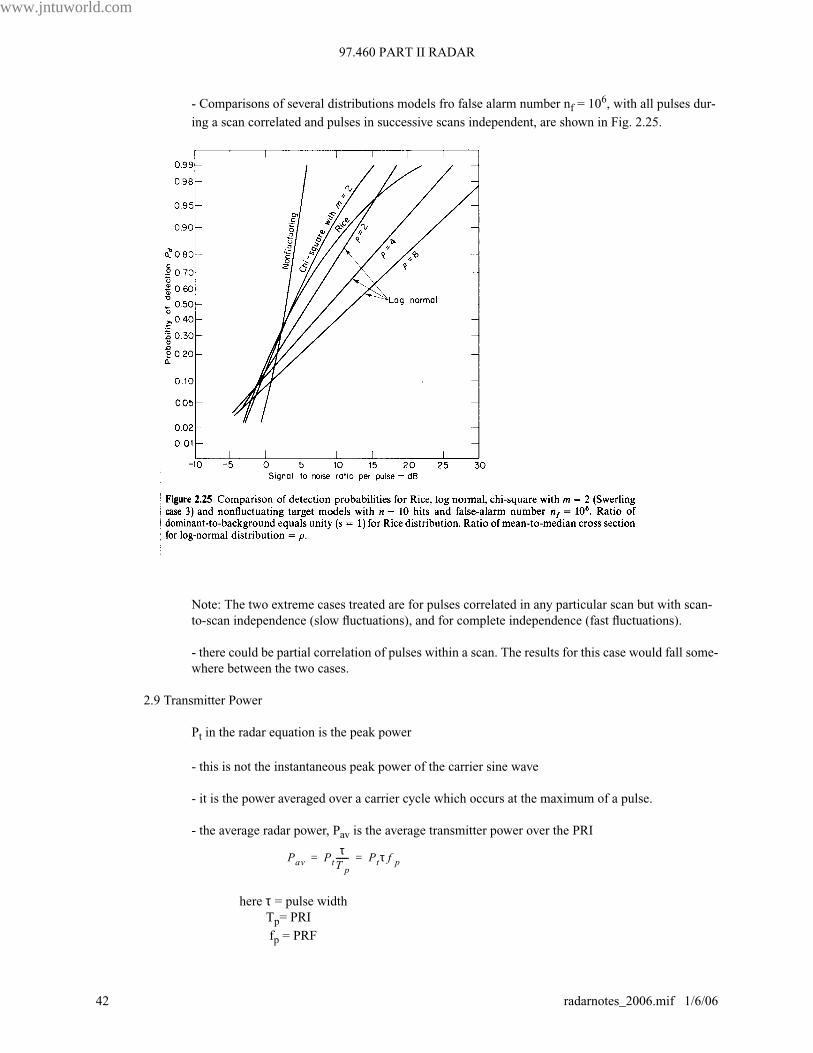
- Comparisons of several distributions models fro false alarm number nf = 106, with all pulses dur-
ing a scan correlated and pulses in successive scans independent, are shown in Fig. 2.25.
Note: The two extreme cases treated are for pulses correlated in any particular scan but with scan-
to-scan independence (slow fluctuations), and for complete independence (fast fluctuations).
- there could be partial correlation of pulses within a scan. The results for this case would fall some-
where between the two cases.
2.9 Transmitter Power
Pt in the radar equation is the peak power
- this is not the instantaneous peak power of the carrier sine wave
- it is the power averaged over a carrier cycle which occurs at the maximum of a pulse.
- the average radar power, Pav is the average transmitter power over the PRI
here τ = pulse width
Tp= PRI
fp = PRF
Pav PtτT p------ Ptτ f p= =
www.jntuworld.com
42 radarnotes_2006.mif 1/6/06
www.jntuworld.com
JNTUWORLD
now which defines the duty cycle
- the typical duty cycle for a surveillance radar is 0.001
- Thus the range equation in terms of average power is
here (Bnτ) are grouped together since the product is usually of the order of unity for pulse radars
- if the transmitted waveform is not a rectangular pulse, we can express the range equation in terms
of energy
Note: In this form Rmax does not depend explicitly on λ or fp
2.10 Pulse Repetition Frequency and Range Ambiguities
- PRF is determined primarily by the maximum range at which targets are expected
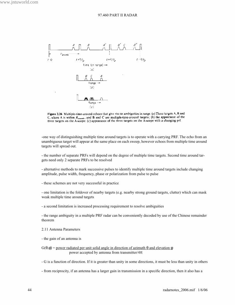
- echoes received after an interval exceeding the PRI are called “multiple-time-around” echoes
- these can result in erroneous range measurements
- consider three targets A, B and C. here A is within the maximum unambiguous range Runambig, B is
between Runambig and 2Runambig and C is between 2Runambig and 3Runambig
PavPt
--------τT p-------=
Rmax4 PavGAeσnEi n( )
4π( )2kT
0Bnτ( )Fn S N⁄( )
1f p
-------------------------------------------------------------------------=
EτPav
fp
--------=
Rmax4 EτGAeσnEi n( )
4π( )2kT
0Bnτ( )Fn S N⁄( )
1
-----------------------------------------------------------------=
www.jntuworld.com
radarnotes_2006.mif 1/6/06 43
97.460 PART II RADAR
www.jntuworld.com
JNTUWORLD
-one way of distinguishing multiple time around targets is to operate with a carrying PRF. The echo from an
unambiguous target will appear at the same place on each sweep, however echoes from multiple time around
targets will spread out.
- the number of separate PRFs will depend on the degree of multiple time targets. Second time around tar-
gets need only 2 separate PRFs to be resolved
- alternative methods to mark successive pulses to identify multiple time around targets include changing
amplitude, pulse width, frequency, phase or polarization from pulse to pulse
- these schemes are not very successful in practice
- one limitation is the foldover of nearby targets (e.g. nearby strong ground targets, clutter) which can mask
weak multiple time around targets
- a second limitation is increased processing requirement to resolve ambiguities
- the range ambiguity in a multiple PRF radar can be conveniently decoded by use of the Chinese remainder
theorem
2.11 Antenna Parameters
- the gain of an antenna is
G(θ,φ) = power radiated per unit solid angle in direction of azimuth θ and elevation φpower accepted by antenna from transmitter/4π
- G is a function of direction. If it is greater than unity in some directions, it must be less than unity in others
- from reciprocity, if an antenna has a larger gain in transmission in a specific direction, then it also has a
www.jntuworld.com
44 radarnotes_2006.mif 1/6/06
www.jntuworld.com
JNTUWORLD
larger effective area in that direction
- the most common beam shapes fro radar are the pencil beam and the fan beam
- pencil beams are axially symmetric with a width of a few degrees. They are used where it is necessary to
measure the angular position of a target continuously in azimuth and elevation (e.g. a tracking radar for
weapons control or missile guidance). These are generated with parabolic reflectors.
- to search a large sector of sky with a narrow beam is difficult. Operational requirements place restrictions
on the maximum scan time (time for beam to return to the same point) so that the radar can not dwell too
long at any particular cell.
- to reduce the number of cells, the pencil beam is replaced with the fan beam which is narrow in one dimen-
sion and wide in the other.
- fan beams can be generated with parabolic reflectors with a shaped projected area. many long range ground
based radars use fan beams
- even with fan beams, a trade-off exists between the rate at which the target position is updated (scan time)
and the ability to detect weak signals (by use of pulse integration)
- scan rates are typically from 1 to 60 rpm
- for long range surveillance, scan rates are typically 5 or 6 rpm
- coverage of a simple fan beam is not adequate for targets at high altitudes close to the radar.
- the elevation pattern is usually shaped to radiate more energy at high angles as in the csc2 pattern.
-here for φ0 < φ< φm
here φ0 and φm are the angular limits of the csc2 φ fit
- this pattern is used for airborne search radars observing ground targets as well as ground based radars
observing aircraft. For the airborne case φ is the depression angle
- ldeally φm should be 90˚ but it is always less
- csc2 φpatterns can be generated by a distorted section of a parabola or with special multiple horn feed on a
true parabola, or with an array such as a slotted waveguide
- the csc2 φ pattern gives constant echo power Pr independent of range for a target of constant height, h and
having a constant σ.
- substituting into the range equation (simple form)
G φ( ) G φ0
( ) φcsc2
φ0
csc2
-----------------=
PrPtG
2 φ0
( ) φ( )csc2λ2σ
4π( )3 φ0
( )csc2R
4----------------------------------------------------- K
1
φ( )csc
R4
----------------= =
www.jntuworld.com
radarnotes_2006.mif 1/6/06 45
97.460 PART II RADAR
www.jntuworld.com
JNTUWORLD
- now for a constant height, h of a target, we have
therefore
- hence the echo signal is independent of range
- in practice Pr varies due to σ varying with viewing angle, the earth not being flat and non perfect csc2 φpat-
terns
Note: the gain of csc2 φ antennas for ground based radars is about 2 dB less than for a fan beam having the
same aperture
- the maximum gain of any antenna is related to its size by
where ρ is the antenna efficiency which depends on the aperture illumination
- this is controlled by the complexity of the feed design
- Note: Aρ = Aeff
- a typical reflector gives a beam width of
where l is the dimension
2.12 System Losses
- losses in the radar reduce the S/N at the receiver output
- losses which can be calculated include the antenna beam shape loss, the collapsing loss and the plumbing
loss
- losses which cannot be calculated readily include those due to field degradation, operator fatigue and lack
of operator motivation
Note: loss has a value greater than unity - Loss = [Gain]-1
Plumbing Loss
φ( )csc R h⁄=
PrK
1
h4
------- K2
= =
G4πA
λ2----------ρ=
θ deg( ) 65λl
---------=
www.jntuworld.com
46 radarnotes_2006.mif 1/6/06

www.jntuworld.com
JNTUWORLD
- loss in transmission lines between the transmitter and antenna and between antenna and receiver
- note from the Fig 2.28 that, at low frequencies, the transmission lines introduce little loss. At high
frequencies the attenuation is significant
- additional loss occurs at connectors (0.5 dB), bends (0.1dB) and at rotary joints (0.4 dB)
Note: if a line is used for both transmission and reception, its loss is added twice
- the duplexer typically adds 1.5 dB insertion loss. In general, the greater the isolation required, the
greater the insertion loss
Beam Shape Loss
- the train of pulses returned from the target to a scanning radar are modulated in amplitude by the
shape of the antenna beam
- a beam shape loss accounts for the fact that the maximum gain is used in the radar equation rather
than a gain which changes from pulse to pulse. (this approach is approximate since it does not
address Pd for each pulse separately)
- let the one way power pattern be approximated by a Gaussian shape
here θB is the half power beam width
S2 2.78θ2
–
θB2
-------------------exp=
www.jntuworld.com
radarnotes_2006.mif 1/6/06 47
97.460 PART II RADAR
www.jntuworld.com
JNTUWORLD
- nB is the number of pulses received within θB and if n is the number of pulses integrated, then the
beam shape loss (relative to a radar that integrated n pulses with equal gain) is
Example integrating 11 pulses gives L (beam shape) = 1.66 dB
Note: the beam shape loss above was for a beam shaped in one plane only (i.e. fan beam or pencil
beam where the target passes through the centre of the beam)
- If the target passe through any other part of the beam the maximum signal will not correspond to
the signal from the beam centre
- when many pulses are integrated per beamwidth, the scanning loss is taken as 1.6 dB for a fan
beam scanning in one coordinate, and as 3.2 dB when two coordinate scanning is used
- when the antenna scans so rapidly that the gain on transmission is not the same as the gain on
reception, an additional “scanning loss” is added.
- additional loss for phased array search using a step scanning pencil beam since not all regions of
space are illuminated by the same value of antenna gain.
Limiting Loss
- limiting in radar can lower the Pd
- this is not a desirable effect and is due to a limited dynamic range
- limiting can be due to pulse compression processing and intensity modulation of CRT (such as
PPI)
- limiting results in a loss of only a fraction of a dB for large numbers of pulses integrated providing
the limiting ratio (ratio of video limit level to RMS noise level) is greater than 2
- for small SNR in bandpass limiters, the reduction of SNR of a sine wave in narrowband Gaussian
noise is π/4 (approx 1 dB)
- if the spectrum of the input noise is shaped correctly, this loss can be made negligible
Collapsing Loss
- if the radar integrates additional noise samples along with the wanted signal +noise pulses, the
added noise causes degradation called the collapsing g loss
- this occurs on displays which collapse range information (C scope which displays El vs Az)
- in some 3D radars (range, Az, El) that display outputs at all Elevations on one PPI (range, Az) dis-
play, the collapsing of the 3D information into 2 D display results in loss
- can also occur when the output of a high resolution radar is displayed on a device which is of
L beamshape( ) n
1 2 5.55k2
–( ) nB2⁄( )exp
k 1=
n 1–( ) 2⁄
∑+
---------------------------------------------------------------------------------=
www.jntuworld.com
48 radarnotes_2006.mif 1/6/06

www.jntuworld.com
JNTUWORLD
coarser resolution than the radar
- Marcum has shown that for a square law detector, the integration of m noise pulses, along with n
signal + noise pulses with SNR per pulse (S/N)n, is equivalent to the integration of m+n signal _
noise pulses each with SNR of
- the collapsing loss then is the ratio of the integration loss Li for m+n pulses to the integration loss
foe n pulses
- recall
Example: 10 signal pulses are integrated with 30 noise pulses
Required Pd = 0.9, nf = 108
From Fig 2.8b
Li (40) = 3.5 dB
Li (10) = 1.7 dB
therefore Li (m,n) = 1.8 dB
- collapsing loss for a linear detector can be much greater than for a square law detector
- Fig 2.29 shows the comparison of loss for each detector
SN----
m n+( )equiv
nm n+-------------
SN )-------
n
=
Li m n,( )Li m n+( )Li n( )
-----------------------=
Li n( ) 1
Ei n( )-------------=
www.jntuworld.com
radarnotes_2006.mif 1/6/06 49
97.460 PART II RADAR
www.jntuworld.com
JNTUWORLD
Nonideal Equipment
- transmitter power - the power varies from tube to tube (for same type), and with age for a specific
tube. Power is also not uniform over the operating band
- hence Pt may be other than the design value.
- to allow for this, a loss factor of about 2 dB can be used
- receiver noise figure - the NF will vary over the band, hence if the best NF is used in the radar
equation, a loss factor must account for its poorer value elsewhere in the band
- matched filter - if the receiver is not the exact matched filter fro the transmitted waveform, a loss
of SNR will occur (typically 1 dB)
- threshold level - due to the exponential relationship between Tfa and VT a slight change in VT
can cause significant change to Tfa hence, VT is set slightly higher than calculated to give good Tfa
in the event of circuit drifts. This is equivalent to a loss
Operator Loss
- a distracted, tired, overloaded, poorly trained operator will perform less efficiently
- the operator efficiency factor (empirical) is where Pd is the single scan probabil-
ity of detection
Note: operator loss is not relevant to systems where automatic detection is done
Field Degradation
- when a radar is operated under field conditions, the performance deteriorates even more than can
be accounted for in the above losses.
- factors which cause field degradation are:
- poor training
- weak tubes
- water in the transmission lines
- incorrect mixer crystal current
- deterioration in the receiver NF
- poor TR tube recovery
- loose cable connections
- radars should be designed with BIST (built - in system test) and BITE (built - in test equipment) to
aid in performance monitoring
ρ0
0.7 Pd( )2=
www.jntuworld.com
50 radarnotes_2006.mif 1/6/06
www.jntuworld.com
JNTUWORLD
- a preventative maintenance plan should be used
- BITE parameters to be monitored are
- Pt
- NF of receiver
- Transmitter pulse shape
- recovery time of TR tube
- with no other information available, 3 dB is assumed for field degradation loss
Other Loss Factors
- MTI radars introduce additional loss. The MTI discrimination technique results in complete loss
of sensitivity for certain target values (blind speeds)
- in a radar with overlapping range gates, the gates may be wider than optimum for practical rea-
sons. The additional noise introduced by nonoptimum gate width leads to degradation performance.
- straddling loss accounts for loss in SNR for targets not at the centre of a range gate, or at the cen-
tre of a filter in a multiple bank processor
Propagation Effects
- the radar equation assumes free space propagation
- the earth’s surface and atmosphere have a significant effect on radar performance
- the effects fall into three categories
- attenuation
- refraction by the earth’s atmosphere
- lobe structure caused by interference between the direct wave and the ground reflected
wave
- for most microwave radars, attenuation through the normal atmosphere or through precipitation is
not significant
- however reflection from rain (clutter) is a limiting factor in radar performance in adverse weather
- the deceasing density of atmosphere with altitude results in bending (refraction) of the electro-
magnetic wave. This normally increases the line of sight. the refraction can also be accounted for
by assuming the earth to have a larger radius than actual. A “typical” earth radius is 4/3 actual
radius.
- at times atmospheric conditions create ducting (or super refraction) and increases the radar range
considerably. It is not necessarily desirable since it can not be counted on. Also it degrades MTI
performance by extending the range at which ground clutter is seen.
www.jntuworld.com
radarnotes_2006.mif 1/6/06 51
97.460 PART II RADAR
www.jntuworld.com
JNTUWORLD
- the presence of the earth also breaks the antenna elevation pattern into many lobes. this arises
since the direct and reflected waves interfere at the target either destructively or constructively to
produce nulls or lobes. This results in non uniform illumination.
2.14 Other Considerations
- the radar equation is now written
Note: The following substitutions can be made:
Eτ = Pav/fp = Ptτ
N0 = N/B (power spectral density of noise)
Bτ ≈ 1
T0Fn = Ts
Note: The above radar equation was derived for rectangular pulses but applies to other waveforms
provided that matched filter detection is used. The equation can be modified to accommodate CW,
FM-CW, pulse doppler MTI or tracking radar.
Radar Performance Figure - ratio of pulse power of Transmitter to Smin of receiver
- not often used
Blip-Scan ratio - same as single scan Pd
- method used to check performance of ground-based radars
- here an aircraft is flown on a radial course and for each scan of the antenna it is recorded
whether or not a target blip is detected. The ration of the number of scans the target was
seen at a particular range to the total number of scans is the blip scan ratio
- head on and tail on aspects are easiest to provide.
Cumulative Probability of Detection
- if single scan probability of detection id Pd, the probability of detecting a target at least
once during N scans is the cumulative probability of detection
Pc = 1-(1-Pd)N
Note: the variation of Pd with range might have to be taken into account in computing Pc.
- the variation with range based on the cumulative probability of detection can be the 3rd
power rather than the 4th power which is based on a single scan probability
Rmax4 PavG Aρa( )σnEi n( )
4π( )2kT
0Bnτ( )Fn S N⁄( )
1f pLs
-------------------------------------------------------------------------------=
www.jntuworld.com
52 radarnotes_2006.mif 1/6/06
www.jntuworld.com
JNTUWORLD
- in practice Pc is not easy to apply. Furthermore radar operators do not usually report a
detection the first time it is observed (which is required by the definition of Pc). Instead
they report a detection based on threshold crossing on two successive scans, or on two out
of three scans
- for track while scan radars, the measure of performance might be the probability of initi-
ating a target track rather than just probability of detection.
Surveillance Radar Equation
- the radar equation which describes the performance of a radar which dwells on the target for n
pulses is sometimes called the searchlight range equation
- in a search or surveillance radar, the additional constraint that the radar must search a specified
volume of space in a specified time modifies the range equation significantly.
- If Ω represents the angular region to be searched in scan time ts, then we have
where t0 is the time on target = n/fp
Ω0 = solid angle beamwidth
Ω0 ≈ θAθE
where θA is the Azimuth beamwidth
and θE is the Elevation beamwidth
also
with these substitutions the range equation becomes
- this indicates that the important parameters for a search radar are the average power and the
antenna effective aperture
- frequency does not appear explicitly, however low frequency is preferred since high power and
large aperture are easier to obtain at low frequency and it is easier to build MTI (moving target indi-
cator) and weather has little effect on performance.
Note: the radar equation will be considerably different if clutter or external noise (jamming) rather
than receiver noise determine the background for the signal
ts t0
ΩΩ
0
-------=
G 4πΩ
0
-------=
Rmax4 PavAeσEi n( )ts
4πkT0Fn S N⁄( )
1LsΩ
------------------------------------------------------=
www.jntuworld.com
radarnotes_2006.mif 1/6/06 53
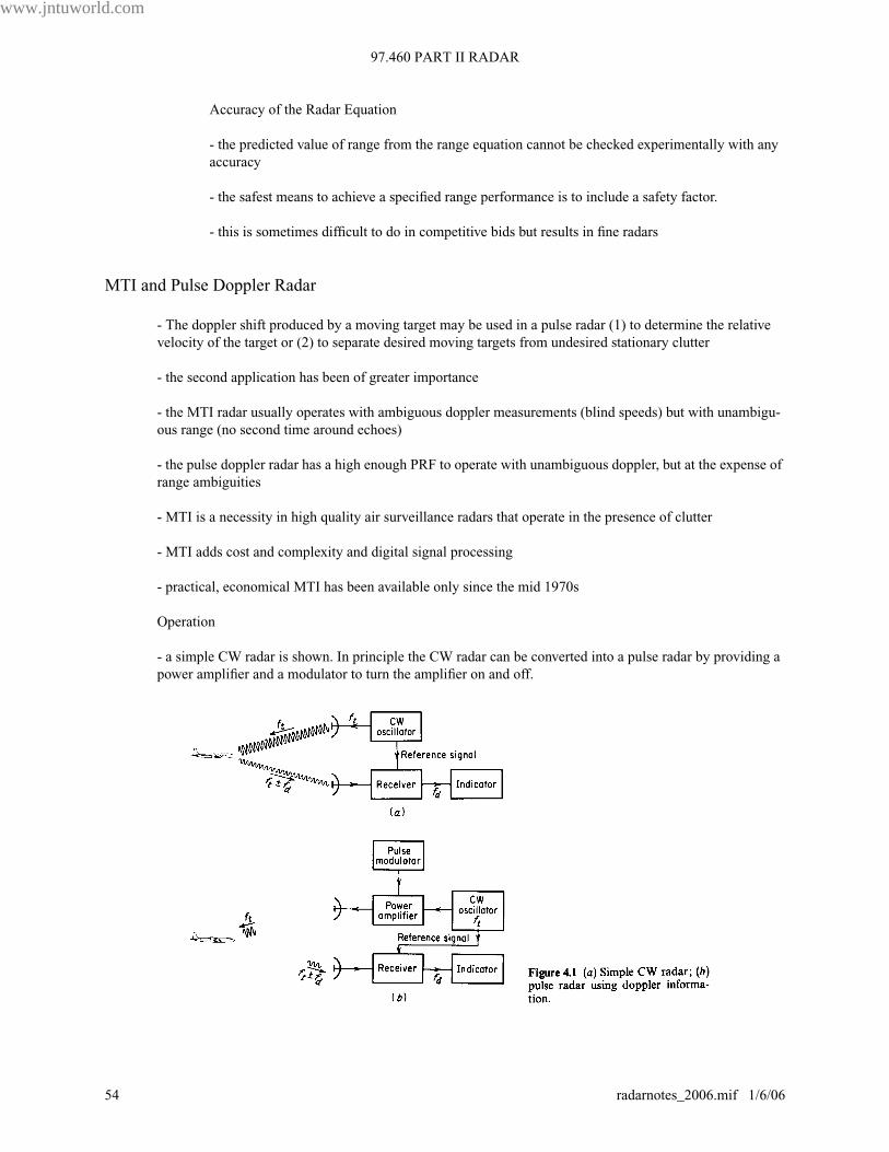
97.460 PART II RADAR
www.jntuworld.com
JNTUWORLD
Accuracy of the Radar Equation
- the predicted value of range from the range equation cannot be checked experimentally with any
accuracy
- the safest means to achieve a specified range performance is to include a safety factor.
- this is sometimes difficult to do in competitive bids but results in fine radars
MTI and Pulse Doppler Radar
- The doppler shift produced by a moving target may be used in a pulse radar (1) to determine the relative
velocity of the target or (2) to separate desired moving targets from undesired stationary clutter
- the second application has been of greater importance
- the MTI radar usually operates with ambiguous doppler measurements (blind speeds) but with unambigu-
ous range (no second time around echoes)
- the pulse doppler radar has a high enough PRF to operate with unambiguous doppler, but at the expense of
range ambiguities
- MTI is a necessity in high quality air surveillance radars that operate in the presence of clutter
- MTI adds cost and complexity and digital signal processing
- practical, economical MTI has been available only since the mid 1970s
Operation
- a simple CW radar is shown. In principle the CW radar can be converted into a pulse radar by providing a
power amplifier and a modulator to turn the amplifier on and off.
www.jntuworld.com
54 radarnotes_2006.mif 1/6/06
www.jntuworld.com
JNTUWORLD
Note: The main difference between this pulse radar and the one described previously is that some portion of
the CW power that generates the transmitted pulse is applied to the receiver as the local oscillator.
- this LO provides the coherent reference needed for doppler frequency detection.
- Coherent means that the phase of the transmitted signal is preserved in the reference signal.
- let the CW oscillator voltage be
- therefore the reference voltage is
(1)
- the doppler shifted echo voltage is
(2)
here c = velocity of propagation
R0 = range of target
- the reference and echo signal are mixed in the receiver and the difference extracted
(3)
Note: equations 2 and 3 represent carriers upon which the pulse modulation is imposed
Note: for stationary targets, fd = 0 therefore Vdiff will have a constant value somewhere between -A4 and A4.
- examples of Vdiff are shown in figure 4.2
- when fd > 1/τ the doppler can be discerned from the information in a single pulse (4.2 b)
- when fd < 1/τ the pulses will be modulated an amplitude given by equation 3 (Fig 4.2.c)
V A1
2π f ttsin=
V ref A2
2π f ttsin=
V echo A3
2π f t f d±( )t4π f tR0
c-------------------–sin=
Vdiff A4
2π f dt4π f tR0
c-------------------–sin=
www.jntuworld.com
radarnotes_2006.mif 1/6/06 55
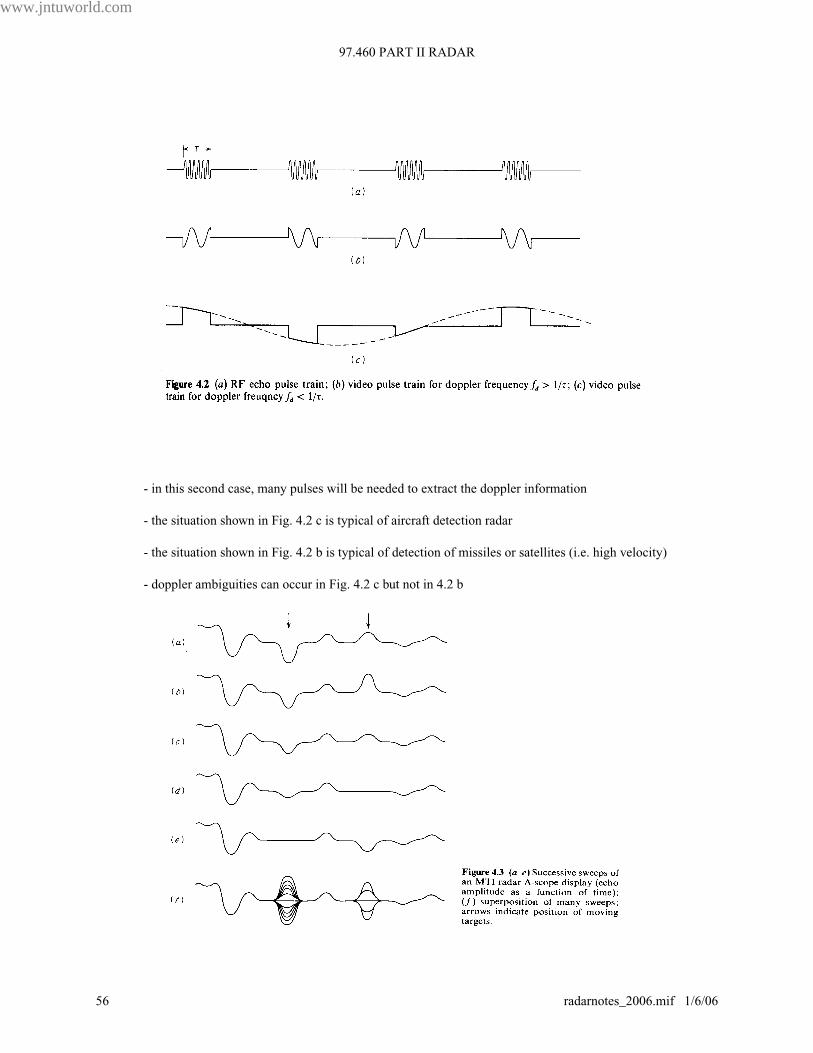
97.460 PART II RADAR
www.jntuworld.com
JNTUWORLD
- in this second case, many pulses will be needed to extract the doppler information
- the situation shown in Fig. 4.2 c is typical of aircraft detection radar
- the situation shown in Fig. 4.2 b is typical of detection of missiles or satellites (i.e. high velocity)
- doppler ambiguities can occur in Fig. 4.2 c but not in 4.2 b
www.jntuworld.com
56 radarnotes_2006.mif 1/6/06
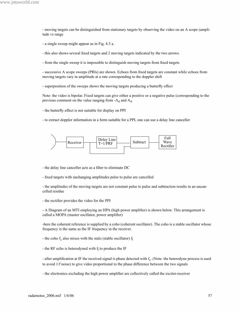
www.jntuworld.com
JNTUWORLD
- moving targets can be distinguished from stationary targets by observing the video on an A scope (ampli-
tude vs range
- a single sweep might appear as in Fig. 4.3 a.
- this also shows several fixed targets and 2 moving targets indicated by the two arrows.
- from the single sweep it is impossible to distinguish moving targets from fixed targets
- successive A scope sweeps (PRIs) are shown. Echoes from fixed targets are constant while echoes from
moving targets vary in amplitude at a rate corresponding to the doppler shift
- superposition of the sweeps shows the moving targets producing a butterfly effect
Note: the video is bipolar. Fixed targets can give either a positive or a negative pulse (corresponding to the
previous comment on the value ranging from -A4 and A4.
- the butterfly effect is not suitable for display on PPI
- to extract doppler information in a form suitable for a PPI, one can use a delay line canceller
- the delay line canceller acts as a filter to eliminate DC
- fixed targets with unchanging amplitudes pulse to pulse are cancelled
- the amplitudes of the moving targets are not constant pulse to pulse and subtraction results in an uncan-
celled residue
- the rectifier provides the video for the PPI
- A Diagram of an MTI employing an HPA (high power amplifier) is shown below. This arrangement is
called a MOPA (master oscillator, power amplifier)
-here the coherent reference is supplied by a coho (coherent oscillator). The coho is a stable oscillator whose
frequency is the same as the IF frequency in the receiver.
- the coho fc also mixes with the stalo (stable oscillator) fl
- the RF echo is heterodyned with fl to produce the IF
- after amplification at IF the received signal is phase detected with fc. (Note: the heterodyne process is used
to avoid 1/f noise) to give video proportional to the phase difference between the two signals
- the electronics excluding the high power amplifier are collectively called the exciter-receiver
ReceiverDelay LineT=1/PRF Subtract
FullWave
Rectifier
www.jntuworld.com
radarnotes_2006.mif 1/6/06 57
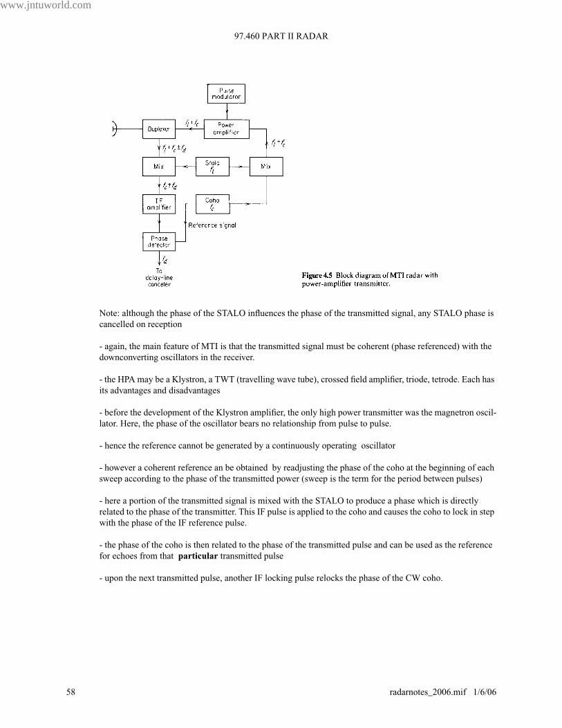
97.460 PART II RADAR
www.jntuworld.com
JNTUWORLD
Note: although the phase of the STALO influences the phase of the transmitted signal, any STALO phase is
cancelled on reception
- again, the main feature of MTI is that the transmitted signal must be coherent (phase referenced) with the
downconverting oscillators in the receiver.
- the HPA may be a Klystron, a TWT (travelling wave tube), crossed field amplifier, triode, tetrode. Each has
its advantages and disadvantages
- before the development of the Klystron amplifier, the only high power transmitter was the magnetron oscil-
lator. Here, the phase of the oscillator bears no relationship from pulse to pulse.
- hence the reference cannot be generated by a continuously operating oscillator
- however a coherent reference an be obtained by readjusting the phase of the coho at the beginning of each
sweep according to the phase of the transmitted power (sweep is the term for the period between pulses)
- here a portion of the transmitted signal is mixed with the STALO to produce a phase which is directly
related to the phase of the transmitter. This IF pulse is applied to the coho and causes the coho to lock in step
with the phase of the IF reference pulse.
- the phase of the coho is then related to the phase of the transmitted pulse and can be used as the reference
for echoes from that particular transmitted pulse
- upon the next transmitted pulse, another IF locking pulse relocks the phase of the CW coho.
www.jntuworld.com
58 radarnotes_2006.mif 1/6/06

www.jntuworld.com
JNTUWORLD
Delay Line Cancellers
- the time domain delay-line canceller capability depends on the quality of the medium used as the delay line
- the delay required is equal to the PRI and might be several milliseconds (long!!!)
- this can not be achieved with electromagnetic transmission lines
- converting the electromagnetic signal to an acoustic signal allows the design of delay lines with reasonable
physical length since the velocity of acoustic waves is approximately 10-5 that of electromagnetic waves.
- the signal at the output of the acoustic delay device is then converted back to an electromagnetic wave.
- solid fused quartz using multiple internal reflections to obtain a compact device were developed in the
1950’s
- these analog delay lines have been replaced by digital delay lines using A/D and digital processing
- the use of digital processing allows implementation of complex delay line cancellers which were not prac-
tical with the analog methods.
Note: An advantage of the time domain delay line canceler as compared with the frequency domain filter is
that a single network operates at all ranges and does not need a separate filter for each range resolution cell.
Filter Characteristics of a Delay Line Canceler
- the canceler acts as a filter to reject DC clutter but because of its periodic nature it also rejects energy near
the PRF and its harmonics
www.jntuworld.com
radarnotes_2006.mif 1/6/06 59
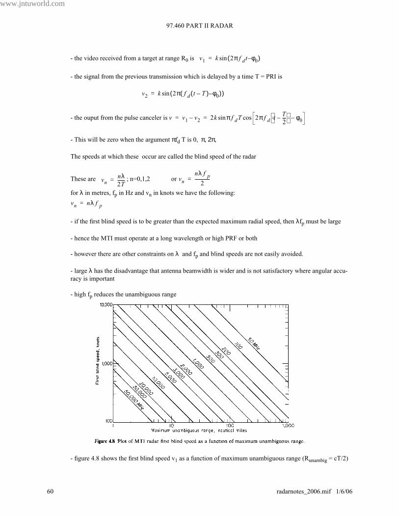
97.460 PART II RADAR
www.jntuworld.com
JNTUWORLD
- the video received from a target at range R0 is
- the signal from the previous transmission which is delayed by a time T = PRI is
- the ouput from the pulse canceler is
- This will be zero when the argument πfd T is 0, π, 2π,
The speeds at which these occur are called the blind speed of the radar
These are ; n=0,1,2 or
for λ in metres, fp in Hz and vn in knots we have the following:
- if the first blind speed is to be greater than the expected maximum radial speed, then λfp must be large
- hence the MTI must operate at a long wavelength or high PRF or both
- however there are other constraints on λ and fp and blind speeds are not easily avoided.
- large λ has the disadvantage that antenna beamwidth is wider and is not satisfactory where angular accu-
racy is important
- high fp reduces the unambiguous range
- figure 4.8 shows the first blind speed v1 as a function of maximum unambiguous range (Runambig = cT/2)
v1
k 2π f dt φ0
–( )sin=
v2
k 2π f d t T–( ) φ0
–( )( )sin=
v v1
v2
– 2k π f dT 2π f d t T2---–
φ0
–cossin= =
vnnλ2T-------= vn
nλ f p2
--------------=
vn nλ f p=
www.jntuworld.com
60 radarnotes_2006.mif 1/6/06

www.jntuworld.com
JNTUWORLD
Example:
- in practice MTI radars in L and S band are designed for the detection of aircraft and must operate with
blind speeds if they are to operate with unambiguous range
- systems which require good MTI performance must operate with ambiguous range (pulse doppler radar)
- the effect of blind speeds can be reduced by operating with more than one PRF (staggered PRF MTI)
-operating at more than one RF frequency can also reduce effect of blind speeds.
Double Cancellation
- single delay line cancelers do not always have as broad a clutter reject null at DC as might be desired
- the null can be widened by the use of cancelers as shown
- in Fig 4.9a, the output of the two single delay line cancellers in cascade is the square of that from a single
delay canceler
- the response of this double delay line canceler is shown in Fig. 4.10.The finite width of the typical clutter
spectrum is also shown to illustrate the additional cancellation offered
- the two delay line canceler of Fig. 4.9b has the same frequency response characteristic as the double delay
line canceler
Table 2:
Runambig f
130 NM 200 MHz
13 NM 3 GHz
4 NM 10 GHz
v 4 π f dT( )sin2
=
www.jntuworld.com
radarnotes_2006.mif 1/6/06 61
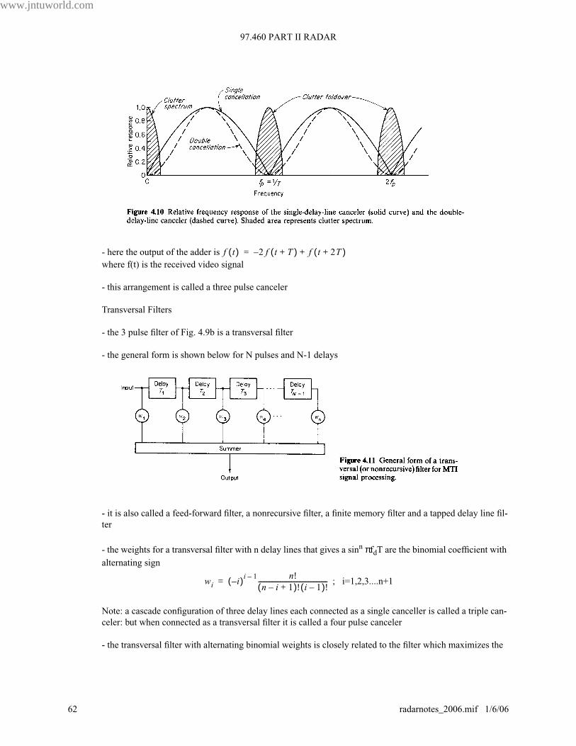
97.460 PART II RADAR
www.jntuworld.com
JNTUWORLD
- here the output of the adder is
where f(t) is the received video signal
- this arrangement is called a three pulse canceler
Transversal Filters
- the 3 pulse filter of Fig. 4.9b is a transversal filter
- the general form is shown below for N pulses and N-1 delays
- it is also called a feed-forward filter, a nonrecursive filter, a finite memory filter and a tapped delay line fil-
ter
- the weights for a transversal filter with n delay lines that gives a sinn πfdT are the binomial coefficient with
alternating sign
; i=1,2,3....n+1
Note: a cascade configuration of three delay lines each connected as a single canceller is called a triple can-
celer: but when connected as a transversal filter it is called a four pulse canceler
- the transversal filter with alternating binomial weights is closely related to the filter which maximizes the
f t( ) 2 f t T+( ) f t 2T+( )+–=
wi i–( )i 1– n!n i– 1+( )! i 1–( )!
--------------------------------------------=
www.jntuworld.com
62 radarnotes_2006.mif 1/6/06
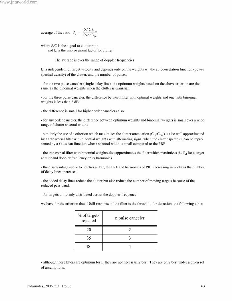
www.jntuworld.com
JNTUWORLD
average of the ratio
where S/C is the signal to clutter ratio
and Ic is the improvement factor for clutter
The average is over the range of doppler frequencies
Ic is independent of target velocity and depends only on the weights wi, the autocorrelation function (power
spectral density) of the clutter, and the number of pulses.
- for the two pulse canceler (single delay line), the optimum weights based on the above criterion are the
same as the binomial weights when the clutter is Gaussian.
- for the three pulse canceler, the difference between filter with optimal weights and one with binomial
weights is less than 2 dB.
- the difference is small for higher order cancelers also
- for any order canceler, the difference between optimum weights and binomial weights is small over a wide
range of clutter spectral widths
- similarly the use of a criterion which maximizes the clutter attenuation (Cin/Cout) is also well approximated
by a transversal filter with binomial weights with alternating signs, when the clutter spectrum can be repre-
sented by a Gaussian function whose spectral width is small compared to the PRF
- the transversal filter with binomial weights also approximates the filter which maximizes the Pd for a target
at midband doppler frequency or its harmonics
- the disadvantage is due to notches at DC, the PRF and harmonics of PRF increasing in width as the number
of delay lines increases
- the added delay lines reduce the clutter but also reduce the number of moving targets because of the
reduced pass band.
- for targets uniformly distributed across the doppler frequency:
we have for the criterion that -10dB response of the filter is the threshold for detection, the following table:
- although these filters are optimum for Ic they are not necessarily best. They are only best under a given set
of assumptions.
% of targets
rejectedn pulse canceler
20 2
35 3
48! 4
I cS C⁄( )outS C⁄( )in
-----------------------=
www.jntuworld.com
radarnotes_2006.mif 1/6/06 63

97.460 PART II RADAR
www.jntuworld.com
JNTUWORLD
- it would seem that the MTI filter should be shaped to reject the clutter at DC and around the PRF, but have
a flat response over the region where no clutter is expected.
- the transversal filter can be designed to achieve this desirable filter response but needs a large number of
delay lines. This sets a restriction on the radar’s PRF, beamwidth, antenna rotation rate and dwell time
- Fig 4.12 shows the amplitude response of a 3 pulse canceler with sin2 πfdT(1), a 5 pulse “optimum” can-
celer which maximizes Ic (2) and a 15 pulse Chebyshev filter (3)
- even a 5 pulse Chebyshev design gives a significantly wider bandwidth than the 5 pulse optimum design
Note: the Chebyshev design has a lower Ic but is worthwhile if the clutter spectrum is narrow
- when there are only a few pulses available for processing, there is little that can be done to control the filter
shape
- hence for 3 or 4 pulse cancelers it is best to use the classical sin2 or sin4 response of the binomial cancelers.
Shaping the Frequency Response
- non recursive filters employ only feedforward loops. These yield zeroes for synthesizing the frequency
response
- if feedback loops are used, each delay line can provide one pole as well as one zero
- the canonical form is shown below:
Fig.4.12
www.jntuworld.com
64 radarnotes_2006.mif 1/6/06
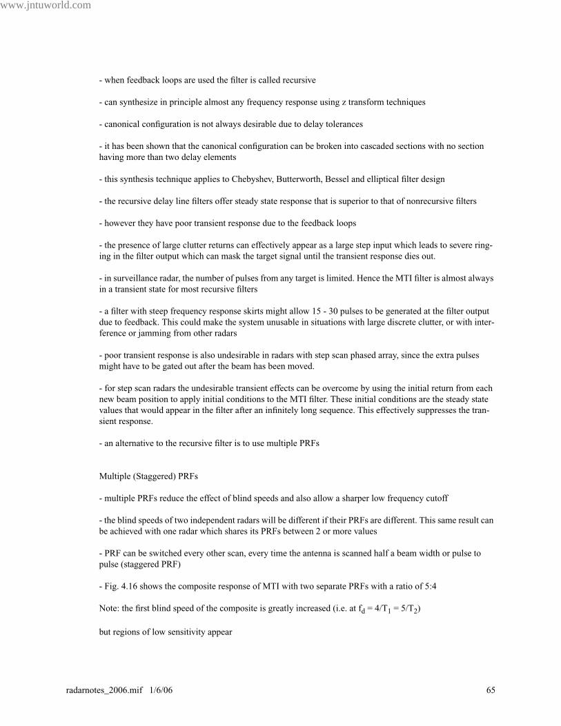
www.jntuworld.com
JNTUWORLD
- when feedback loops are used the filter is called recursive
- can synthesize in principle almost any frequency response using z transform techniques
- canonical configuration is not always desirable due to delay tolerances
- it has been shown that the canonical configuration can be broken into cascaded sections with no section
having more than two delay elements
- this synthesis technique applies to Chebyshev, Butterworth, Bessel and elliptical filter design
- the recursive delay line filters offer steady state response that is superior to that of nonrecursive filters
- however they have poor transient response due to the feedback loops
- the presence of large clutter returns can effectively appear as a large step input which leads to severe ring-
ing in the filter output which can mask the target signal until the transient response dies out.
- in surveillance radar, the number of pulses from any target is limited. Hence the MTI filter is almost always
in a transient state for most recursive filters
- a filter with steep frequency response skirts might allow 15 - 30 pulses to be generated at the filter output
due to feedback. This could make the system unusable in situations with large discrete clutter, or with inter-
ference or jamming from other radars
- poor transient response is also undesirable in radars with step scan phased array, since the extra pulses
might have to be gated out after the beam has been moved.
- for step scan radars the undesirable transient effects can be overcome by using the initial return from each
new beam position to apply initial conditions to the MTI filter. These initial conditions are the steady state
values that would appear in the filter after an infinitely long sequence. This effectively suppresses the tran-
sient response.
- an alternative to the recursive filter is to use multiple PRFs
Multiple (Staggered) PRFs
- multiple PRFs reduce the effect of blind speeds and also allow a sharper low frequency cutoff
- the blind speeds of two independent radars will be different if their PRFs are different. This same result can
be achieved with one radar which shares its PRFs between 2 or more values
- PRF can be switched every other scan, every time the antenna is scanned half a beam width or pulse to
pulse (staggered PRF)
- Fig. 4.16 shows the composite response of MTI with two separate PRFs with a ratio of 5:4
Note: the first blind speed of the composite is greatly increased (i.e. at fd = 4/T1 = 5/T2)
but regions of low sensitivity appear
www.jntuworld.com
radarnotes_2006.mif 1/6/06 65

97.460 PART II RADAR
www.jntuworld.com
JNTUWORLD
- the closer the ratio T1: T2 approaches unity, the greater the frequency of the first blind speed, and the
deeper he first null in the vicinity of fd - 1/T1.
- the null depth can be reduced and the first blind speed increased by operating with more than 2 PRFs
- Fig 4.17 shows a five pulse stagger (4 periods) response with periods in the ratio 25:30:27:31
www.jntuworld.com
66 radarnotes_2006.mif 1/6/06
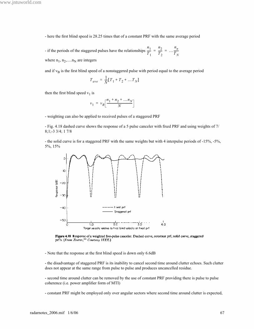
www.jntuworld.com
JNTUWORLD
- here the first blind speed is 28.25 times that of a constant PRF with the same average period
- if the periods of the staggered pulses have the relationships
where n1, n2,.....nN are integers
and if vB is the first blind speed of a nonstaggered pulse with period equal to the average period
then the first blind speed v1 is
- weighting can also be applied to received pulses of a staggered PRF
- Fig. 4.18 dashed curve shows the response of a 5 pulse canceler with fixed PRF and using weights of 7/
8;1;-3 3/4; 1 7/8
- the solid curve is for a staggered PRF with the same weights but with 4 interpulse periods of -15%, -5%,
5%, 15%
- Note that the response at the first blind speed is down only 6.6dB
- the disadvantage of staggered PRF is its inability to cancel second time around clutter echoes. Such clutter
does not appear at the same range from pulse to pulse and produces uncancelled residue.
- second time around clutter can be removed by the use of constant PRF providing there is pulse to pulse
coherence (i.e. power amplifier form of MTI)
- constant PRF might be employed only over angular sectors where second time around clutter is expected,
n1
T1
------n
2
T2
------ …nnTN-------= =
Tave1
N---- T
1T
2…TN+ +[ ]=
v1
vBn
1n
2…nN+ +
N-------------------------------------=
www.jntuworld.com
radarnotes_2006.mif 1/6/06 67

97.460 PART II RADAR
www.jntuworld.com
JNTUWORLD
or by changing the PRF each time the antenna scans half a beamwidth, or by changing the PRF each scan
period.
Range Gated Doppler Filters
- it is possible to use frequency domain band pass filters in MTI radar to sort the doppler frequency shifted
targets
- a narrow band filter with a pass band designed to pass the doppler components of a moving target will ring
when excited by a short radar pulse.
- the narrow band filter smears the input pulse since the impulse response is the reciprocal of the filter band-
width. This smearing destroys the range resolution.
- if there are more than one target in the smeared region they can not be resolved
- even for one target, noise from other range cells will interfere (collapsing loss) resulting in reduction in
sensitivity
- the loss of range information and collapsing loss can be eliminated by quantizing the range into small inter-
vals (range gating)
- the width of the range gate is usually of the order of the pulse width
- the range resolution is established by range gating. Once the return is quantized, the output from each gate
is applied to a narrow band filter since the pulse shape need no linger be preserved for range resolution.
- collapsing loss does not take place since noise from other range intervals is excluded.
- the output of the phase detector is sampled sequentially by range gates
- the range gate acts as a switch which opens and closes at the proper time. Gates are activated once each
PRI.
- the output from a stationary target is s series of pulses of constant amplitude
www.jntuworld.com
68 radarnotes_2006.mif 1/6/06
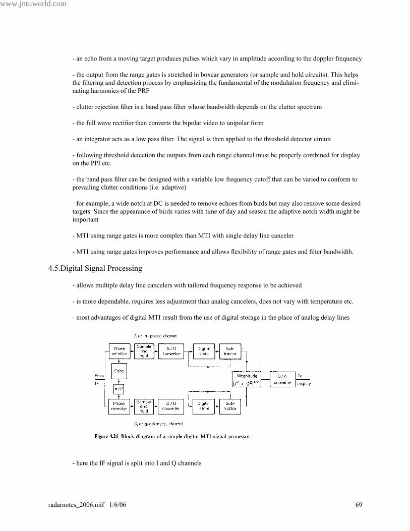
www.jntuworld.com
JNTUWORLD
- an echo from a moving target produces pulses which vary in amplitude according to the doppler frequency
- the output from the range gates is stretched in boxcar generators (or sample and hold circuits). This helps
the filtering and detection process by emphasizing the fundamental of the modulation frequency and elimi-
nating harmonics of the PRF
- clutter rejection filter is a band pass filter whose bandwidth depends on the clutter spectrum
- the full wave rectifier then converts the bipolar video to unipolar form
- an integrator acts as a low pass filter. The signal is then applied to the threshold detector circuit
- following threshold detection the outputs from each range channel must be properly combined for display
on the PPI etc.
- the band pass filter can be designed with a variable low frequency cutoff that can be varied to conform to
prevailing clutter conditions (i.e. adaptive)
- for example, a wide notch at DC is needed to remove echoes from birds but may also remove some desired
targets. Since the appearance of birds varies with time of day and season the adaptive notch width might be
important
- MTI using range gates is more complex than MTI with single delay line canceler
- MTI using range gates improves performance and allows flexibility of range gates and filter bandwidth.
4.5.Digital Signal Processing
- allows multiple delay line cancelers with tailored frequency response to be achieved
- is more dependable, requires less adjustment than analog cancelers, does not vary with temperature etc.
- most advantages of digital MTI result from the use of digital storage in the place of analog delay lines
- here the IF signal is split into I and Q channels
www.jntuworld.com
radarnotes_2006.mif 1/6/06 69

97.460 PART II RADAR
www.jntuworld.com
JNTUWORLD
- the outputs of the two phase detectors are 90˚ out of phase
- the quadrature channel eliminates the effects of blind phases. Note that this is seldom done in analog delay
line cancelers due to the complexity involved with additional analog delay lines.
- the baseband bipolar video is sampled at a rate to obtain one or more samples per range resolution cell
- the A/D output is stored in the memory for one PRI and then subtracted from the words from the next
sweep
- the I and Q outputs are combined as either or
- the combined output is then converted to an analog signal with D/A for display
Note: more complex filtering schemes are normally implemented.
- the memory can be RAM or a shift register
- A/D must operate at high speeds to preserve the information content, and also have sufficient number of
bits to quantize the signal to preserve precision
- the number of bits determines the maximum improvement factor for the MTI radar
- the A/D converter must cover the peak excursion of the phase detector output. To ensure this, a limiter may
be necessary
- the quantization noise introduced by the A/D imposes a limit to the improvement factor of
where 2N - 1 is the number of discrete intervals
this is approximately 6dB / bit
Example:
a 9 bit A/D has 511 levels
thus the maximum resolution is 1 out of 511
= 54 dB
Note: IQN = 52.9 which is close
- blind phase - this is different from blind speed
- blind speed occurs when pulse sampling occurs at the same point on the doppler cycle at each sampling
instant (Fig 4.22a)
I2
Q2
+ I Q+
IQN 20 2N
1–( ) 0.75[ ]log≈
I 20511
1---------log=
www.jntuworld.com
70 radarnotes_2006.mif 1/6/06
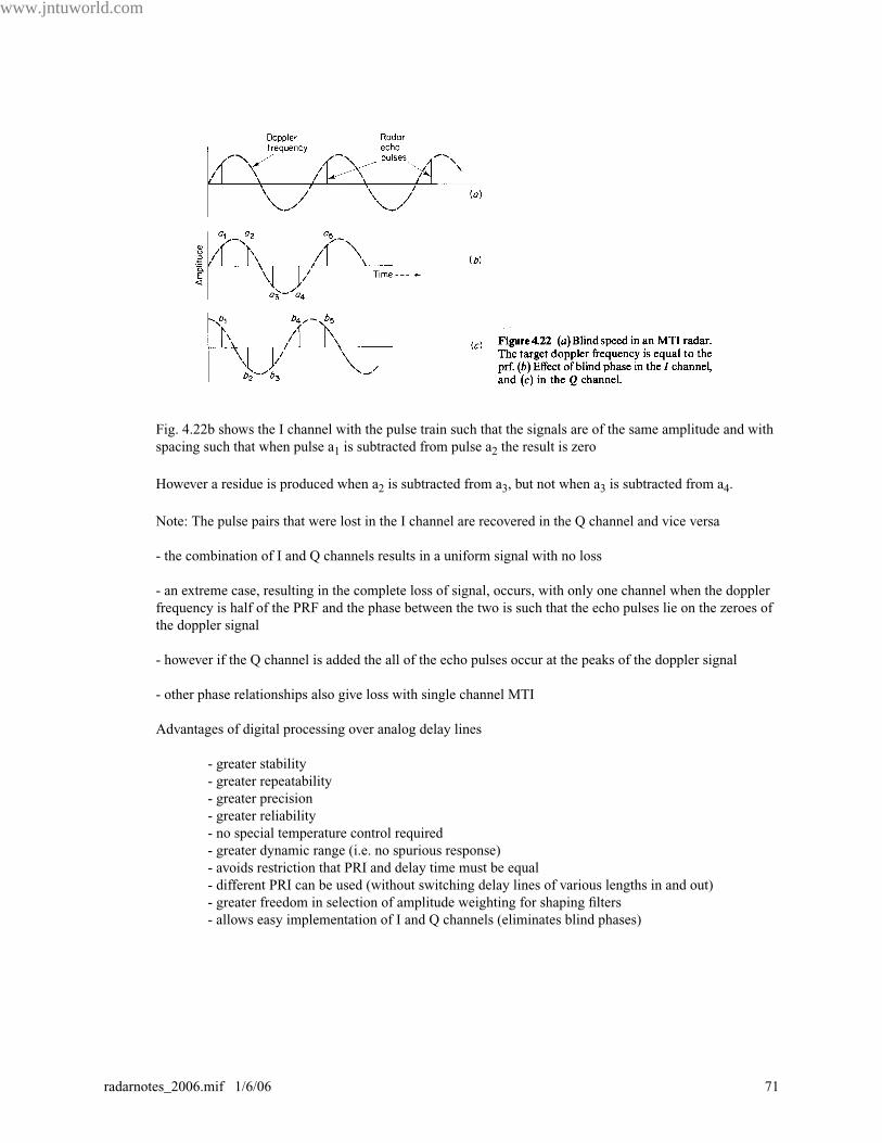
www.jntuworld.com
JNTUWORLDFig. 4.22b shows the I channel with the pulse train such that the signals are of the same amplitude and with
spacing such that when pulse a1 is subtracted from pulse a2 the result is zero
However a residue is produced when a2 is subtracted from a3, but not when a3 is subtracted from a4.
Note: The pulse pairs that were lost in the I channel are recovered in the Q channel and vice versa
- the combination of I and Q channels results in a uniform signal with no loss
- an extreme case, resulting in the complete loss of signal, occurs, with only one channel when the doppler
frequency is half of the PRF and the phase between the two is such that the echo pulses lie on the zeroes of
the doppler signal
- however if the Q channel is added the all of the echo pulses occur at the peaks of the doppler signal
- other phase relationships also give loss with single channel MTI
Advantages of digital processing over analog delay lines
- greater stability
- greater repeatability
- greater precision
- greater reliability
- no special temperature control required
- greater dynamic range (i.e. no spurious response)
- avoids restriction that PRI and delay time must be equal
- different PRI can be used (without switching delay lines of various lengths in and out)
- greater freedom in selection of amplitude weighting for shaping filters
- allows easy implementation of I and Q channels (eliminates blind phases)
www.jntuworld.com
radarnotes_2006.mif 1/6/06 71
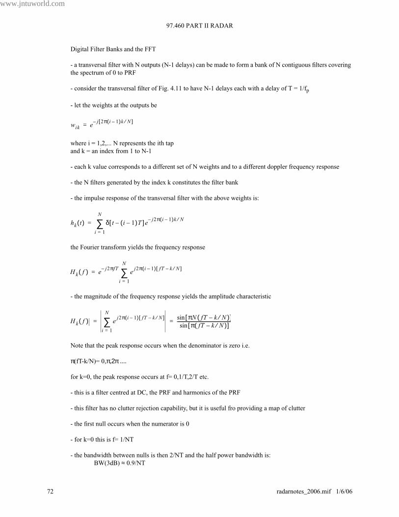
97.460 PART II RADAR
www.jntuworld.com
JNTUWORLD
Digital Filter Banks and the FFT
- a transversal filter with N outputs (N-1 delays) can be made to form a bank of N contiguous filters covering
the spectrum of 0 to PRF
- consider the transversal filter of Fig. 4.11 to have N-1 delays each with a delay of T = 1/fp
- let the weights at the outputs be
where i = 1,2,... N represents the ith tap
and k = an index from 1 to N-1
- each k value corresponds to a different set of N weights and to a different doppler frequency response
- the N filters generated by the index k constitutes the filter bank
- the impulse response of the transversal filter with the above weights is:
the Fourier transform yields the frequency response
- the magnitude of the frequency response yields the amplitude characteristic
Note that the peak response occurs when the denominator is zero i.e.
π(fT-k/N)= 0,π,2π ....
for k=0, the peak response occurs at f= 0,1/T,2/T etc.
- this is a filter centred at DC, the PRF and harmonics of the PRF
- this filter has no clutter rejection capability, but it is useful fro providing a map of clutter
- the first null occurs when the numerator is 0
- for k=0 this is f= 1/NT
- the bandwidth between nulls is then 2/NT and the half power bandwidth is:
BW(3dB) ≈ 0.9/NT
wik ej 2π i 1–( )k N⁄[ ]–
=
hk t( ) δ t i 1–( )T–[ ] e j2π i 1–( )k N⁄–
i 1=
N
∑=
Hk f( ) ej2πfT–
ej2π i 1–( ) fT k N⁄–[ ]
i 1=
N
∑=
Hk f( ) ej2π i 1–( ) fT k N⁄–[ ]
i 1=
N
∑ πN fT k N⁄–( )[ ]sin
π fT k N⁄–( )[ ]sin--------------------------------------------------= =
www.jntuworld.com
72 radarnotes_2006.mif 1/6/06
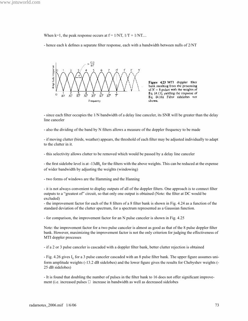
www.jntuworld.com
JNTUWORLD
When k=1, the peak response occurs at f = 1/NT, 1/T + 1/NT....
- hence each k defines a separate filter response, each with a bandwidth between nulls of 2/NT
- since each filter occupies the 1/N bandwidth of a delay line canceler, its SNR will be greater than the delay
line canceler
- also the dividing of the band by N filters allows a measure of the doppler frequency to be made
- if moving clutter (birds, weather) appears, the threshold of each filter may be adjusted individually to adapt
to the clutter in it.
- this selectivity allows clutter to be removed which would be passed by a delay line canceler
- the first sidelobe level is at -13dBc for the filters with the above weights. This can be reduced at the expense
of wider bandwidth by adjusting the weights (windowing)
- two forms of windows are the Hamming and the Hanning
- it is not always convenient to display outputs of all of the doppler filters. One approach is to connect filter
outputs to a “greatest of” circuit, so that only one output is obtained (Note: the filter at DC would be
excluded)
- the improvement factor for each of the 8 filters of a 8 filter bank is shown in Fig. 4.24 as a function of the
standard deviation of the clutter spectrum, for a spectrum represented as a Gaussian function.
- for comparison, the improvement factor for an N pulse canceler is shown in Fig. 4.25
Note: the improvement factor for a two pulse canceler is almost as good as that of the 8 pulse doppler filter
bank. However, maximizing the improvement factor is not the only criterion for judging the effectiveness of
MTI doppler processes
- if a 2 or 3 pulse canceler is cascaded with a doppler filter bank, better clutter rejection is obtained
- Fig. 4.26 gives Ic for a 3 pulse canceler cascaded with an 8 pulse filter bank. The upper figure assumes uni-
form amplitude weights (-13.2 dB sidelobes) and the lower figure gives the results for Chebyshev weights (-
25 dB sidelobes)
- It is found that doubling the number of pulses in the filter bank to 16 does not offer significant improve-
ment (i.e. increased pulses ⇒ increase in bandwidth as well as decreased sidelobes
www.jntuworld.com
radarnotes_2006.mif 1/6/06 73
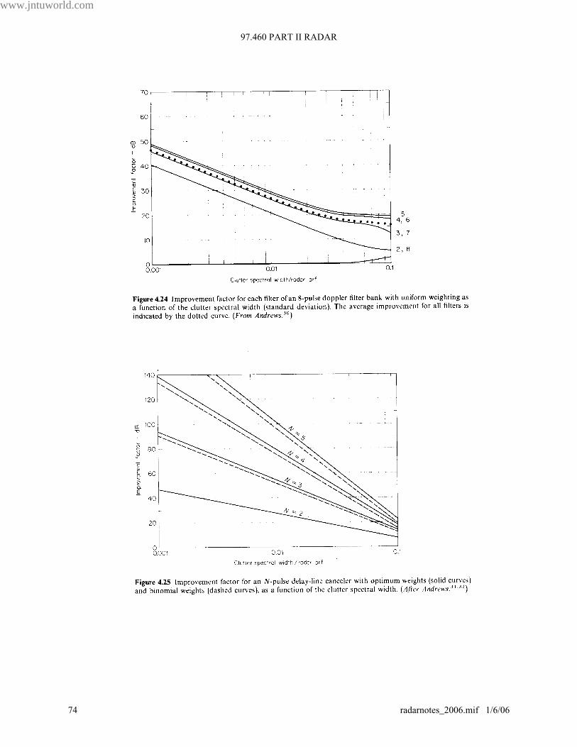
97.460 PART II RADAR
www.jntuworld.com
JNTUWORLD
www.jntuworld.com
74 radarnotes_2006.mif 1/6/06
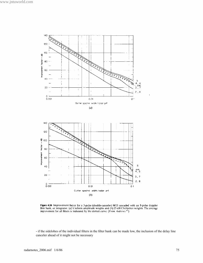
www.jntuworld.com
JNTUWORLD
- if the sidelobes of the individual filters in the filter bank can be made low, the inclusion of the delay line
canceler ahead of it might not be necessary
www.jntuworld.com
radarnotes_2006.mif 1/6/06 75

97.460 PART II RADAR
www.jntuworld.com
JNTUWORLD
4.6 Other MTI Delay Lines
- solid crystal has been mentioned previously
- electrostatic storage tube
- here the signals are stored on a mesh similar to that of a TV camera. The first sweep reads the sig-
nal on the storage tube. the next sweep written on the same space and generates the difference
between the two. Two tubes are required; one to write and store the new sweep, the other to subtract
the new sweep from the old. The electrostatic storage tube can be used with different PRFs
- the charge transfer device (CTD) is a sampled data, analog shift register which can be used as a delay line,
transversal filter and recursive filter
- there are two types of CTD;
- the bucket brigade device (BBD) with capacitive storage elements separated by switches. Here the
data is transferred through the BBD at a rate determined by the rate at which the switches are oper-
ated. The delay time is determined by the number of stages and the switching (or clock) speed.
- charge coupled devices (CCDs) are similar except that charge packets are transferred to adjacent
potential wells by a clocked potential gradient
Notes: - the sampling frequency must give one or two samples per resolution cell
- no A/D or D/A required as for digital systems
- MTI cancelling can be done at IF. Here no blind phases occur
- finally the video can FM modulate a carrier f
or acoustic delay. This avoids problems of amplitude stability of acoustic delay lines.
4.7 Example of an MTI Radar Processor
- the moving target detector (MTD) was developed by Lincoln Labs for the FAA’s airport surveillance radars
(ASR)
- the ASR is a medium range (60 NM) radar located at most US airports.
- it has 2.7 to 2.9 GHz RF, 1µs pulse width, 1.4 ˚ azimuth beamwidth, antenna rotation rate of 12.5 to 15
RPM PRF from 700 to 1200 Hz and average power from 400 to 600 W.
- the MTD processor is based on digital technology.
- uses a 3 pulse canceler followed by an 8 pulse FFT doppler filter bank with weighting to reduce sidelobes
- the total system has alternating PRFs to eliminate blind speeds, adaptive thresholds and a clutter map used
for detecting targets with zero radial speed.
www.jntuworld.com
76 radarnotes_2006.mif 1/6/06
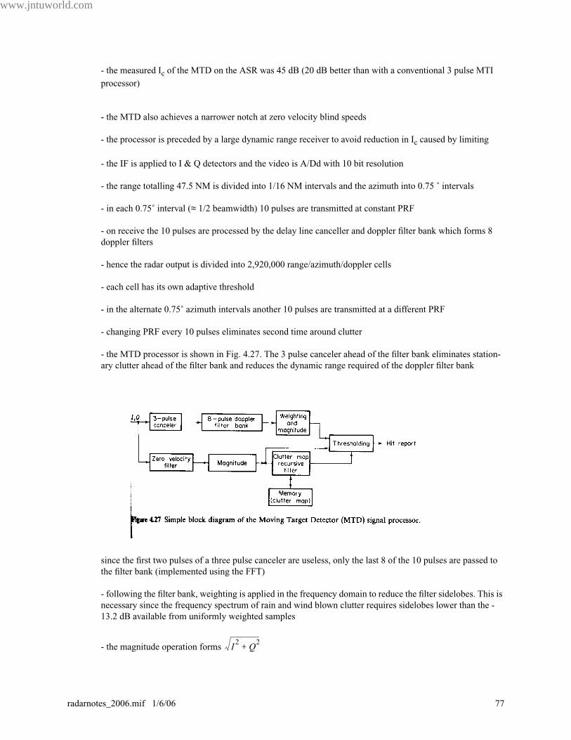
www.jntuworld.com
JNTUWORLD
- the measured Ic of the MTD on the ASR was 45 dB (20 dB better than with a conventional 3 pulse MTI
processor)
- the MTD also achieves a narrower notch at zero velocity blind speeds
- the processor is preceded by a large dynamic range receiver to avoid reduction in Ic caused by limiting
- the IF is applied to I & Q detectors and the video is A/Dd with 10 bit resolution
- the range totalling 47.5 NM is divided into 1/16 NM intervals and the azimuth into 0.75 ˚ intervals
- in each 0.75˚ interval (≈ 1/2 beamwidth) 10 pulses are transmitted at constant PRF
- on receive the 10 pulses are processed by the delay line canceller and doppler filter bank which forms 8
doppler filters
- hence the radar output is divided into 2,920,000 range/azimuth/doppler cells
- each cell has its own adaptive threshold
- in the alternate 0.75˚ azimuth intervals another 10 pulses are transmitted at a different PRF
- changing PRF every 10 pulses eliminates second time around clutter
- the MTD processor is shown in Fig. 4.27. The 3 pulse canceler ahead of the filter bank eliminates station-
ary clutter ahead of the filter bank and reduces the dynamic range required of the doppler filter bank
since the first two pulses of a three pulse canceler are useless, only the last 8 of the 10 pulses are passed to
the filter bank (implemented using the FFT)
- following the filter bank, weighting is applied in the frequency domain to reduce the filter sidelobes. This is
necessary since the frequency spectrum of rain and wind blown clutter requires sidelobes lower than the -
13.2 dB available from uniformly weighted samples
- the magnitude operation forms I2
Q2
+
www.jntuworld.com
radarnotes_2006.mif 1/6/06 77
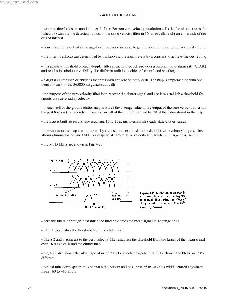
97.460 PART II RADAR
www.jntuworld.com
JNTUWORLD
- separate thresholds are applied to each filter. For non zero velocity resolution cells the thresholds are estab-
lished by scanning the detected outputs of the same velocity filter in 16 range cells, eight on either side of the
cell of interest
- hence each filter output is averaged over one mile in range to get the mean level of non zero velocity clutter
- the filter thresholds are determined by multiplying the mean levels by a constant to achieve the desired Pfa
- this adaptive threshold on each doppler filter at each range cell provides a constant false alarm rate (CFAR)
and results in subclutter visibility (for different radial velocities of aircraft and weather)
- a digital clutter map establishes the thresholds for zero velocity cells. The map is implemented with one
word for each of the 365000 range/azimuth cells
- the purpose of the zero velocity filter is to recover the clutter signal and use it to establish a threshold for
targets with zero radial velocity
- in each cell of the ground clutter map is stored the average value of the output of the zero velocity filter for
the past 8 scans (32 seconds) On each scan 1/8 of the output is added to 7/8 of the value stored in the map
- the map is built up recursively requiring 10 to 20 scans to establish steady state clutter values
- the values in the map are multiplied by a constant to establish a threshold for zero velocity targets. This
allows elimination of usual MTI blind speed at zero relative velocity for targets with large cross section
- the MTD filters are shown in Fig. 4.28
- here the filters 3 through 7 establish the threshold from the mean signal in 16 range cells
- filter 1 establishes the threshold from the clutter map
- filters 2 and 8 adjacent to the zero velocity filter establish the threshold from the larger of the mean signal
over 16 range cells and the clutter map
- Fig 4.28 also shows the advantage of using 2 PRFs to detect targets in rain. As shown, the PRFs are 20%
different.
- typical rain storm spectrum is shown o the bottom and has about 25 to 30 knots width centred anywhere
from - 60 to +60 knots
www.jntuworld.com
78 radarnotes_2006.mif 1/6/06
www.jntuworld.com
JNTUWORLD
- an aircraft return is also shown at the right of the figure and is shown as occupying filters 6 and 7 on PRF-1
and filters 7 and 8 on PRF-2 (the difference is due to frequency foldover)
- with PRF-2 the aircraft velocity is competing with the rain clutter, but at PRF-1 it is clear of clutter.
- hence by using 2 PRFs alternating every 10 pulses, aircraft targets will appear in at least one filter free of
rain (except when the aircraft’s radial velocity is that of the rain)
- interference from other radars may appear as one large return among the ten returns processed
- the MTD has an interference eliminator which compares the magnitude of each of the ten pulses against
the average magnitude of the ten pulses. If any pulse is greater than 5 times the average, all information from
that range/azimuth cell is discarded
- the output of the MTD is a hit report containing azimuth, range, amplitude, filter number and PRF
- on one scan, a large aircraft might be reported from more than one doppler filter, from several coherent pro-
cessing intervals and from adjacent range cells
- up to 20 hit reports might be generated from a single large target
- a post processor groups together all reports which appear to originate from the same target and interpolates
to find the best azimuth, range, amplitude and radar velocity
- target amplitude and doppler are used to eliminate small cross section and low speed angle echoes before
targets are delivered to the automatic tracking circuits.
- tracking circuits eliminate false hit reports which do not form logical tracks
- the output of the automatic tracker is what is displayed on the PPI.
- since the MTD processor eliminates large amounts of clutter and has a low false detection rate, its output
can be remoted via narrow bandwidth telephone
4. 8 Limitations of MTI Performance
- improvement in signal to clutter is affected by factors other than the doppler spectrum
- instabilities in the transmitter and receiver, physical motion of the clutter, finite time on target and receiver
limiting all affect Ic.
Definitions
- MTI Improvement Factor, I
The signal to clutter ratio at the output of the MTI system divided by the signal to clutter ratio at the
input, averaged over all of the target radial velocities of interest
- Subclutter Visibility (SCV):
The ratio by which the target echo may be weaker than the coincident clutter echo power and still
be detected with specified Pd and Pfa. All target radial velocities are assumed equally likely
www.jntuworld.com
radarnotes_2006.mif 1/6/06 79

97.460 PART II RADAR
www.jntuworld.com
JNTUWORLD
Note: A typical value is 30 dB
Note: two radars with the same subclutter visibility might not have the same ability to detect targets
in clutter if the resolution cell of one is greater and accepts more clutter echo power
- Clutter Visibility Factor Voc
- the signal to clutter ratio after cancellation (or doppler processing) that provides the stated Pd and
Pfa
- Clutter Attenuation CA
- the ratio of the clutter power at the canceler input to the clutter residue at the output, normalized
(divided by) to the attenuation of a single pulse passing through the unprocessed channel of the
canceler
- Cancellation Ratio
- the ratio of canceler voltage amplification fro fixed target echoes received with a fixed antenna, to
the gain for a single pulse passing through the unprocessed channel of the canceler.
Note:
Note: When the MTI is limited by noiselike system instabilities, Voc should be chosen as the SNR for range
equation calculations
Note: when the MTI is limited by antenna scanning fluctuations, let Voc = 6dB for a single pulse
Note: Once again, I is the preferred measure of MTI performance but does not account for possible poor per-
formance at certain velocities
- Interclutter Visibility
- the ability of the MTI to detect moving targets in clear resolution cells between patches of strong
clutter. Resolution cells can be range, azimuth or doppler
Note: the higher the radar resolution, the better the interclutter visibility. A medium resolution radar with 2
µs pulse width and 1.5 ˚ beamwidth has sufficient resolution to achieve a 20 dB advantage over low resolu-
tion radars
Equipment Instabilities
- the apparent frequency spectrum from perfectly stationary clutter can be broadened (and hence will
degrade the MTI improvement factor) due to the following:
- pulse to pulse changes in amplitude
- pulse to pulse changes in frequency
- pulse to pulse changes in phase
- timing jitter on transient pulse
I c SCV( ) Voc( )=
www.jntuworld.com
80 radarnotes_2006.mif 1/6/06

www.jntuworld.com
JNTUWORLD
- variations in time delay through the delay lines
- changes in pulse width
- changes in coho or stalo between time of transmit and time of receive
- consider the effect of phase variations.
- let the echo from a stationary clutter on pulse 1 and pulse 2 be
where ∆φ is the change in oscillator phase between the two pulses
- On subtraction
- hence the limitation on the improvement factor due to oscillator instability is
Note: to achieve I > 40 dB requires ∆φ < 0.01 rad from pulse to pulse!. This applies to the coho locking or
the phase change introduced by the HPA
- the limits to I imposed by pulse to pulse instability are:
Transmitter frequency (π∆fτ.)-2
Stalo or coho frequency (2π∆fT)-2
Transmitter phase shift (∆φ)-2
Coho locking (∆φ)-2
Pulse timing τ2/(∆t)22BτPulse width τ2/(∆τ)2BτPulse amplitude (A/∆A)2
where ∆f = interpulse frequency change
B = bandwidth
τ = pulse width
T = transmission time
∆φ = interpulse phase change
∆t = timing jitter
∆τ = pulse width jitter
∆A = interpulse amplitude change
Note: the digital processor does not experience degradation due to timing jitter of the transmit pulse if the
clock controlling the processor timing is started from the detected RF envelope of the transmitted pulse
Internal Fluctuation of Clutter
- absolutely stationary clutter - buildings, water towers, mountains, bare hills
g1
A ωtcos=
g2
A ωt ∆φ+( )cos=
g1t( ) g
2t( )– 2A
∆φ2
------- ωt ∆φ
2-------+
A∆φ ωt ∆φ2
-------+ sin≈sinsin=
I A2
A∆φ( )2------------------
1
∆φ( )2--------------= =
www.jntuworld.com
radarnotes_2006.mif 1/6/06 81
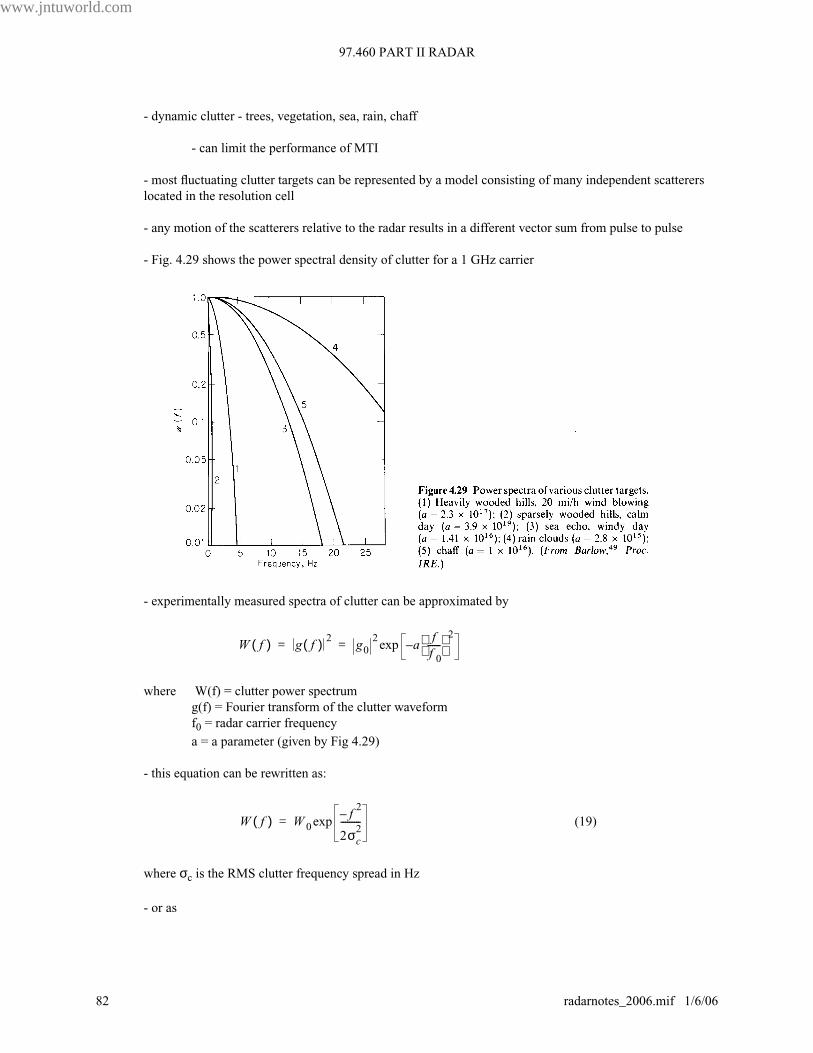
97.460 PART II RADAR
www.jntuworld.com
JNTUWORLD
- dynamic clutter - trees, vegetation, sea, rain, chaff
- can limit the performance of MTI
- most fluctuating clutter targets can be represented by a model consisting of many independent scatterers
located in the resolution cell
- any motion of the scatterers relative to the radar results in a different vector sum from pulse to pulse
- Fig. 4.29 shows the power spectral density of clutter for a 1 GHz carrier
- experimentally measured spectra of clutter can be approximated by
where W(f) = clutter power spectrum
g(f) = Fourier transform of the clutter waveform
f0 = radar carrier frequency
a = a parameter (given by Fig 4.29)
- this equation can be rewritten as:
(19)
where σc is the RMS clutter frequency spread in Hz
- or as
W f( ) g f( ) 2g
0
2a
ff
0
------ 2
–exp= =
W f( ) W0
f2
–
2σc2
---------exp=
www.jntuworld.com
82 radarnotes_2006.mif 1/6/06
www.jntuworld.com
JNTUWORLD
where σv is the clutter velocity spread in m/s
Note:
- the improvement factor can be written as (20)
where CA = Ci/C0 - clutter attenuation averaged over all doppler frequencies
- for a single delay line canceler
(21)
where H(f) is the frequency response of the canceler
- for a single delay line canceler
h(f) = 1- exp(-j2πfT)
= 2jsin(πfT)exp(-jπfT) (22)
- substituting eqn 19 and 22 into 21 gives
assuming σc << 1/T yields
- if the exponential is small, we can use the first two terms of its series expansion
W f( ) W0
f2λ2
–
8σv2
----------------exp=
σc2σvλ
---------=
a c2
8σv2
---------=
IS
0C
0⁄
Si Ci⁄----------------
S0
Si-----
ave
CA= =
CA
W f( ) fd
0
∞
∫
W f( ) H f( ) 2fd
0
∞
∫----------------------------------------------=
CA
W0f( ) f
22σc
2⁄–[ ] fdexp
0
∞
∫
W0
f2
2σc2⁄–[ ] 4 πfT( )sin
2exp fd
0
∞
∫--------------------------------------------------------------------------------------=
CA 0.5
1 2π2T
2σc2
–[ ]exp–---------------------------------------------------=
www.jntuworld.com
radarnotes_2006.mif 1/6/06 83
97.460 PART II RADAR
www.jntuworld.com
JNTUWORLD
or
or
Now the average gain (S0/Si)ave for the single delay line canceler is 2
- hence (25)
- similarly for a double canceler, whose average gain is 6
(26)
- a plot of equation 26 is shown in Fig 4.30 with fpλ as a parameter. Several representative examples of clut-
CAf p
2
4π2σc2
------------------=
CAf p
2 λ2
16π2σv2
---------------------=
CAaf p
2
2π2f
0
2------------------=
I1c
f p2
2π2σc2
---------------f p
2 λ2
8π2σv2
---------------a f p
2
π2f
0
2------------= = =
I2c
f p4
8π4σc4
---------------f p
4 λ4
128π4σv4
----------------------a
2f p
4
2π4f
0
4----------------= = =
www.jntuworld.com
84 radarnotes_2006.mif 1/6/06
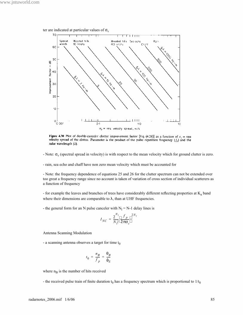
www.jntuworld.com
JNTUWORLD
ter are indicated at particular values of σv
- Note: σv (spectral spread in velocity) is with respect to the mean velocity which for ground clutter is zero.
- rain, sea echo and chaff have non zero mean velocity which must be accounted for
- Note: the frequency dependence of equations 25 and 26 for the clutter spectrum can not be extended over
too great a frequency range since no account is taken of variation of cross section of individual scatterers as
a function of frequency
- for example the leaves and branches of trees have considerably different reflecting properties at Ka band
where their dimensions are comparable to λ, than at UHF frequencies.
- the general form for an N pulse canceler with Nl = N-1 delay lines is
Antenna Scanning Modulation
- a scanning antenna observes a target for time t0
where nB is the number of hits received
- the received pulse train of finite duration t0 has a frequency spectrum which is proportional to 1/t0
I NC2N l
N l!--------
f p2πσc------------
2N l
=
t0
nBf p-------
θBθS------= =
www.jntuworld.com
radarnotes_2006.mif 1/6/06 85
97.460 PART II RADAR
www.jntuworld.com
JNTUWORLD
- hence even if the clutter were perfectly stationary, the clutter spectrum would have a finite width due to the
finite time on target.
- if the clutter spectrum is too wide due to too short an observation interval, the improvement factor will be
affected
- this limitation is called scanning fluctuation or scanning modulation
- to find the limitation on Ic we first find the clutter attenuation CA
here WS(f) describes the spectrum produced by the finite time on target
and H(f) is the MTI processor frequency response
- if the antenna main beam is approximated by a Gaussian shape, the spectrum will also be Gaussian. hence
the results previously derived for a Gaussian clutter spectrum can be applied.
- thus equations 25 and 26 apply for the antenna scanning fluctuations with the correct interpretation of σc
(the RMS spread of the spectrum about the mean)
- here the voltage waveform for the clutter is modulated by the antenna power pattern (equal to the two way
field strength pattern), as it is rotated
now
where θ and θB are in degrees
therefore
where Sa (t) is the modulation of the received signal due to the antenna pattern
and is the scan rate in ˚/s.
CA
WS f( ) fd
0
∞
∫
WS f( ) H f( ) 2fd
0
∞
∫------------------------------------------------=
G θ( ) G0
2.776θ2–
θB2
----------------------exp=
Sa G0
2.776θθs-----
2
–
θBθs------
2
------------------------------exp=
θs
www.jntuworld.com
86 radarnotes_2006.mif 1/6/06

www.jntuworld.com
JNTUWORLD
now and
hence
- the spectrum is found by taking the Fourier transform
=
Since this is a Gaussian function we must have
- hence Note: this is for the voltage spectrum
- for the power spectrum we have
- hence the σs due to the antenna scanning is
- substituting this for σc in equations 25 and 26 yields
single canceler
and
θθs----- t=
θBθs------ t
0=
Sa K2.776t
2–
t0
2---------------------exp=
Sa K2.776t
2–
t0
2--------------------- j2πft–[ ]expexp td
∞–
∞
∫=
K1
π2f
2t0
2–
2.776--------------------exp
π2f
2t0
2–
2.776--------------------
f2
2σ f2
----------=
σ f1.178
πt0
-------------=
σsσ f
2-------=
σs1
3.77t0
---------------=
I1s
nB2
1.388-------------=
I2s
nB4
3.853-------------=
www.jntuworld.com
radarnotes_2006.mif 1/6/06 87

97.460 PART II RADAR
www.jntuworld.com
JNTUWORLD
- Note: the stepped scan antenna also is limited in MTI performance by the finite time on target. The time
waveform is rectangular which gives a different improvement factor.
www.jntuworld.com
88 radarnotes_2006.mif 1/6/06
www.jntuworld.com
JNTUWORLD
Limiting in MTI Radar
- a limiter is used just before the MTI processor to prevent the residue from large clutter echoes from saturat-
ing the display
- ideally an MTI radar should reduce clutter to a level comparable to noise. However, when I is not great
enough, the clutter residue will appear on the display and prevent the detection of aircraft whose radar cross
section is larger than the clutter residue.
- this condition can be prevented by setting the limit L relative to the noise N equal to the MTI improvement
factor I
- if the limit level is set too high, clutter residue obscures part of the display. If the limit is set too low, there
may be a black hole effect
- the limiter provides a CFAR (Constant False Alarm Rate)
- a nonlinear limiter however causes the spectrum of strong clutter to spread into the canceler pass band and
results in the generation of additional residue which degrades the MTI performance.
- Figure 4.32 plots I for 2 pulse and 3 pulse cancelers with various levels of limiting. The abscissa applies to
Gaussian clutter spectrum generated by clutter motion (σv) or by antenna scanning modulation (nB)
- here C/L is the ratio of RMS clutter power to the IF limit level
Note: the loss of I increases with the complexity of the canceler. Limiting in a 3 pulse canceler will cause a
15 to 25 dB reduction in performance. A 4 pulse canceler with limiting is only 2 dB better than a 3 pulse
canceler. Hence adding complexity is not justified in a limiting environment
- limiting is not needed if processor I is large enough to reduce the largest clutter to the noise level (typically
requires I ≈ 60 dB). This is difficult to achieve since it requires the receiver to have a linear dynamic range of
at least 60 dB, the A/D must have at least 11 bits, the equipment must be stable, the processor must be
designed for I = 60 dB and the number of pulses processed must be sufficient to reduce the antenna scanning
modulation
LN---- I=
www.jntuworld.com
radarnotes_2006.mif 1/6/06 89
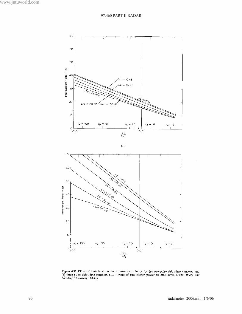
97.460 PART II RADAR
www.jntuworld.com
JNTUWORLD
www.jntuworld.com
90 radarnotes_2006.mif 1/6/06
www.jntuworld.com
JNTUWORLD
5.10 tracking with Surveillance Radar
- the track of a target can be determined with a surveillance radar from the coordinates of the target mea-
sured from scan to scan
- the quality of such a track depends on the time between observations, the location accuracy of each obser-
vation and the number of extraneous targets present in the vicinity of the tracked target
- a surveillance radar which develops tracks on targets it has detected is called a “track while scan” (TWS)
radar
- tracks can be obtained by having an operator mark the location of a target on the face of the PPI with a
grease pencil on each scan
- a single operator however can not handle more than about 6 target tracks when the radar has a twelve sec-
ond scan rate
- also an operator’s effectiveness in detecting new targets decreases rapidly after 1/2 hour of operation
- these problems are avoided by automating the target detection and tracking process. This is called “auto-
matic detection and tracking (ADT)
- the ADT performs the following functions:
- target detection
- track initiation
- track association
- track update
- track smoothing
- track termination
- the automatic detection quantizes the range into intervals equal to the range resolution
- at each range interval the detector integrates n pulses (n is the expected number of hits expected from the
target due to the antenna scan rate)
- the integrated pulses are compared with the threshold to determine the presence or absence of a target
- an example is the “moving window detector” which examines continuously the last n samples within each
quantized range and announces the presence of a target if m out of n of these samples cross a preset thresh-
old
- by locating the centre of the n pulses, an estimate of the target’s angular direction can be obtained. This is
called “beam splitting”
- if there is only one target present within the radar’s coverage, then the detection on two scans is all that is
required to establish a target track and estimate its’ velocity.
- however there are usually other targets plus clutter echoes and hence three or more detections are necessary
to establish a track reliably without the generation of false tracks.
- a computer can recognize and reject false tracks, however too many false tracks can overload a computer
www.jntuworld.com
radarnotes_2006.mif 1/6/06 91
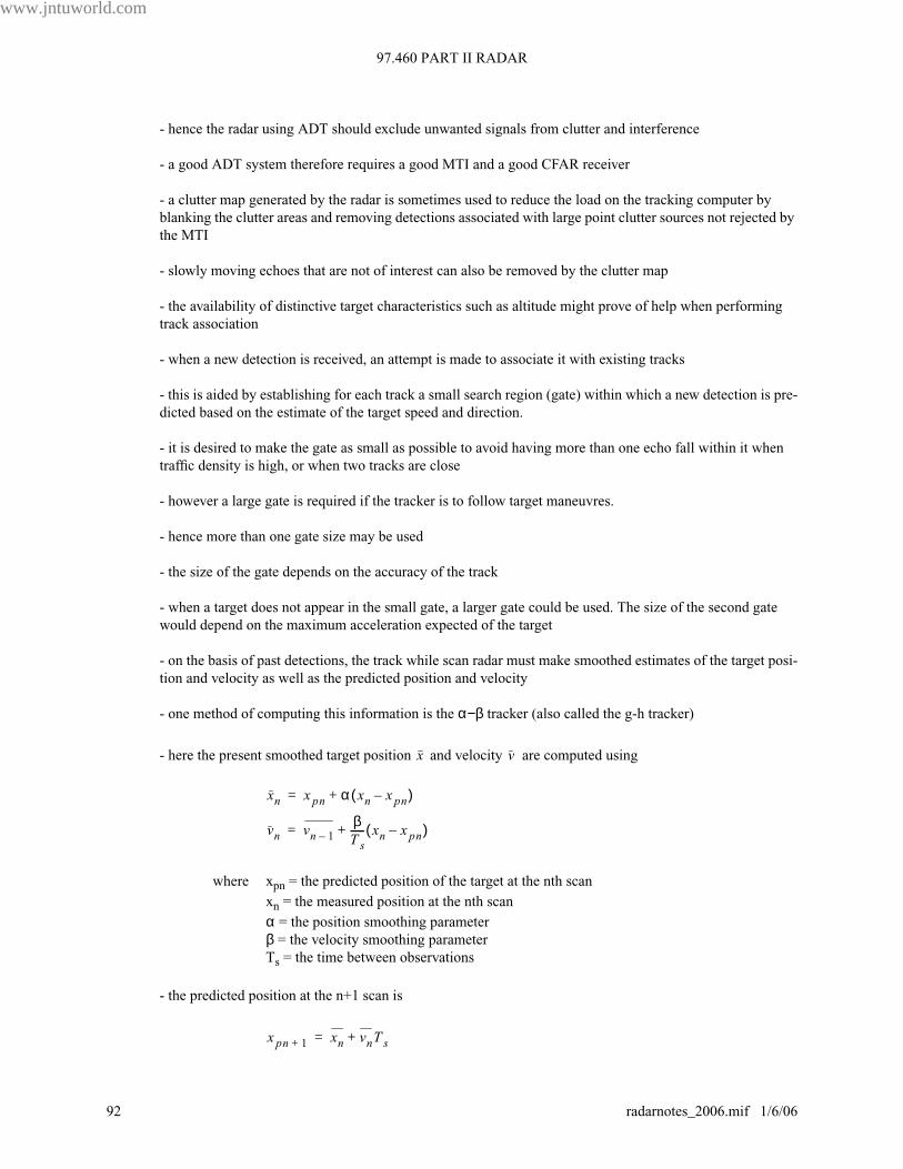
97.460 PART II RADAR
www.jntuworld.com
JNTUWORLD
- hence the radar using ADT should exclude unwanted signals from clutter and interference
- a good ADT system therefore requires a good MTI and a good CFAR receiver
- a clutter map generated by the radar is sometimes used to reduce the load on the tracking computer by
blanking the clutter areas and removing detections associated with large point clutter sources not rejected by
the MTI
- slowly moving echoes that are not of interest can also be removed by the clutter map
- the availability of distinctive target characteristics such as altitude might prove of help when performing
track association
- when a new detection is received, an attempt is made to associate it with existing tracks
- this is aided by establishing for each track a small search region (gate) within which a new detection is pre-
dicted based on the estimate of the target speed and direction.
- it is desired to make the gate as small as possible to avoid having more than one echo fall within it when
traffic density is high, or when two tracks are close
- however a large gate is required if the tracker is to follow target maneuvres.
- hence more than one gate size may be used
- the size of the gate depends on the accuracy of the track
- when a target does not appear in the small gate, a larger gate could be used. The size of the second gate
would depend on the maximum acceleration expected of the target
- on the basis of past detections, the track while scan radar must make smoothed estimates of the target posi-
tion and velocity as well as the predicted position and velocity
- one method of computing this information is the α−β tracker (also called the g-h tracker)
- here the present smoothed target position and velocity are computed using
where xpn = the predicted position of the target at the nth scan
xn = the measured position at the nth scan
α = the position smoothing parameter
β = the velocity smoothing parameter
Ts = the time between observations
- the predicted position at the n+1 scan is
x v
xn x pn α xn x pn–( )+=
vn vn 1–βT s------ xn x pn–( )+=
x pn 1+ xn vnT s+=
www.jntuworld.com
92 radarnotes_2006.mif 1/6/06
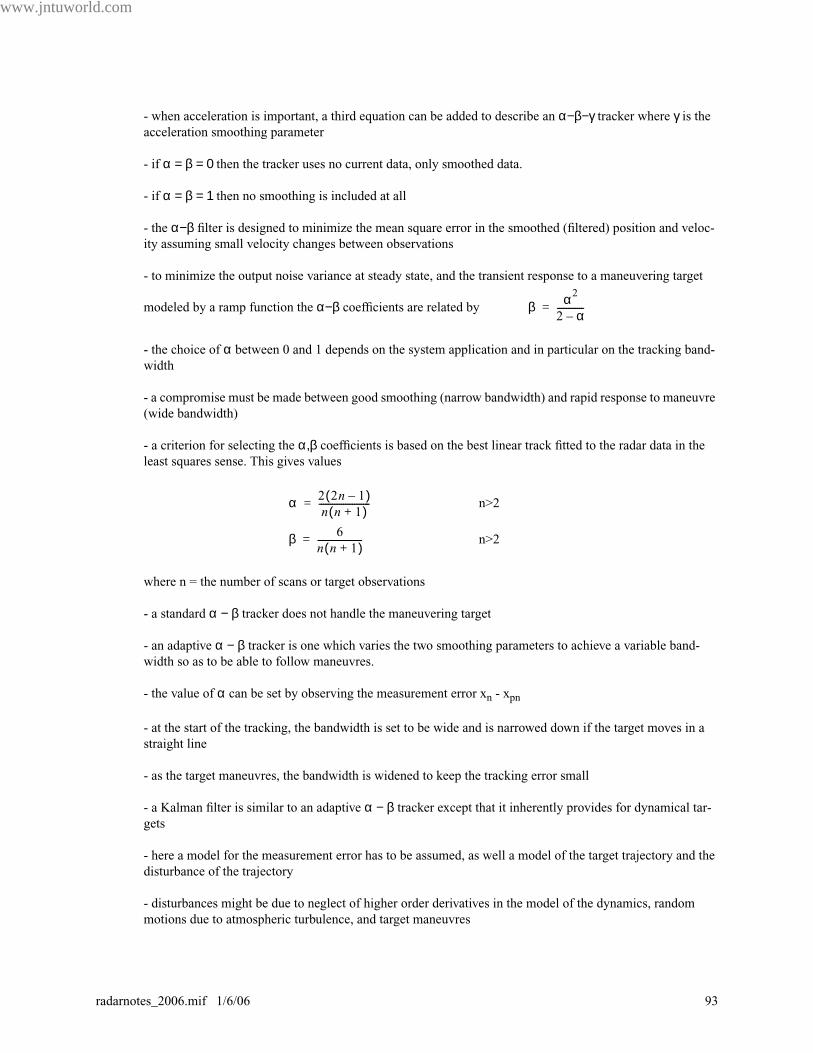
www.jntuworld.com
JNTUWORLD
- when acceleration is important, a third equation can be added to describe an α−β−γ tracker where γ is the
acceleration smoothing parameter
- if α = β = 0 then the tracker uses no current data, only smoothed data.
- if α = β = 1then no smoothing is included at all
- the α−β filter is designed to minimize the mean square error in the smoothed (filtered) position and veloc-
ity assuming small velocity changes between observations
- to minimize the output noise variance at steady state, and the transient response to a maneuvering target
modeled by a ramp function the α−β coefficients are related by
- the choice of α between 0 and 1 depends on the system application and in particular on the tracking band-
width
- a compromise must be made between good smoothing (narrow bandwidth) and rapid response to maneuvre
(wide bandwidth)
- a criterion for selecting the α,β coefficients is based on the best linear track fitted to the radar data in the
least squares sense. This gives values
n>2
n>2
where n = the number of scans or target observations
- a standard α − β tracker does not handle the maneuvering target
- an adaptive α − β tracker is one which varies the two smoothing parameters to achieve a variable band-
width so as to be able to follow maneuvres.
- the value of α can be set by observing the measurement error xn - xpn
- at the start of the tracking, the bandwidth is set to be wide and is narrowed down if the target moves in a
straight line
- as the target maneuvres, the bandwidth is widened to keep the tracking error small
- a Kalman filter is similar to an adaptive α − β tracker except that it inherently provides for dynamical tar-
gets
- here a model for the measurement error has to be assumed, as well a model of the target trajectory and the
disturbance of the trajectory
- disturbances might be due to neglect of higher order derivatives in the model of the dynamics, random
motions due to atmospheric turbulence, and target maneuvres
β α2
2 α–------------=
α 2 2n 1–( )n n 1+( )-----------------------=
β 6
n n 1+( )--------------------=
www.jntuworld.com
radarnotes_2006.mif 1/6/06 93
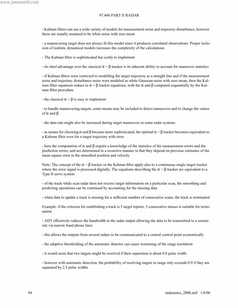
97.460 PART II RADAR
www.jntuworld.com
JNTUWORLD
- Kalman filters can use a wide variety of models for measurement noise and trajectory disturbance, however
these are usually assumed to be white noise with zero mean
- a maneuvering target does not always fit this model since it produces correlated observations. Proper inclu-
sion of realistic dynamical models increases the complexity of the calculations
- The Kalman filter is sophisticated but costly to implement
- its chief advantage over the classical α − β tracker is its inherent ability to account for maneuvre statistics
- if Kalman filters were restricted to modelling the target trajectory as a straight line and if the measurement
noise and trajectory disturbance noise were modeled as white Gaussian noise with zero mean, then the Kal-
man filter equations reduce to α − β tracker equations, with the α and β computed sequentially by the Kal-
man filter procedure
- the classical α − β is easy to implement
- to handle maneuvering targets, some means may be included to detect maneuvres and to change the values
of α and β.
- the data rate might also be increased during target maneuvres in some radar systems
- as means for choosing α and β become more sophisticated, the optimal α − β tracker becomes equivalent to
a Kalman filter even for a target trajectory with error
- here the computation of α and β require a knowledge of the statistics of the measurement errors and the
prediction errors, and are determined in a recursive manner in that they depend on previous estimates of the
mean square error in the smoothed position and velocity
Note: The concept of the α − β tracker or the Kalman filter apply also to a continuous single target tracker
where the error signal is processed digitally. The equations describing the α − β tracker are equivalent to a
Type II servo system
- of the track while scan radar does not receive target information on a particular scan, the smoothing and
predicting operations can be continued by accounting for the missing data
- when data to update a track is missing for a sufficient number of consecutive scans, the track is terminated
Example: if the criterion for establishing a track is 3 target reports, 5 consecutive misses is suitable for termi-
nation
- ADT effectively reduces the bandwidth in the radar output allowing the data to be transmitted to a remote
site via narrow band phone lines
- this allows the outputs from several radars to be communicated to a central control point economically
- the adaptive thresholding of the automatic detector can cause worsening of the range resolution
- it would seem that two targets might be resolved if their separation is about 0.8 pulse width
- however with automatic detection, the probability of resolving targets in range only exceeds 0.9 if they are
separated by 2.5 pulse widths
www.jntuworld.com
94 radarnotes_2006.mif 1/6/06

www.jntuworld.com
JNTUWORLD
- to achieve this resolution, a log video receiver should be used and the threshold should be proportioned to
the smaller of the two means calculated from a number of reference cells on either side of the test cell
- this resolution limit assumes that the shape of the return pulse is not known. (If it were, it would be possible
to resolve targets within one pulse width)
- when more than one radar are covering the same volume of space, it is sometimes desirable to combine
their outputs to form a single track file (Automatic Detection and Integrated Tracking, ADIT)
- ADIT has the advantage of a greater data rate than a single radar and reduces the likelihood of a loss of tar-
get detections caused by antenna lobing, fading, interference and clutter
- the integrated processing allows a favourable weighting of better data and lesser weighting of the poorer
data
www.jntuworld.com
radarnotes_2006.mif 1/6/06 95